Systematic Review on Learning-based Spectral CT

Abstract

Spectral CT has recently emerged as an advanced version of medical CT and significantly improves conventional (single-energy) CT. Spectral CT has two main forms: DECT and PCCT, which offer image improvement, material decomposition, and feature quantification relative to conventional CT. However, the inherent challenges of spectral CT, evidenced by data and image artifacts, remain a bottleneck for clinical applications. To address these problems, machine learning techniques have been widely applied to spectral CT. In this review, we present the state-of-the-art data-driven techniques for spectral CT.

I Introduction

Since Cormack and Hounsfield’s Nobel prize-winning breakthrough, X-ray CT is extensively used in medical applications and produces a huge number of gray-scale CT images. However, these images are often insufficient to distinguish crucial differences between biological tissues and contrast agents. From the perspective of physics, the X-ray spectrum from a medical device is polychromatic, and interactions between X-rays and biological tissues depend on the X-ray energy, which suggests the feasibility to obtain spectral, multi-energy, or true-color, CT images.

Over the past decade, spectral CT has been rapidly developed as a new generation of CT technology. DECT and PCCT are the two main forms of spectral CT. DECT is a method of acquiring two projection datasets at different energy levels. PCCT, on the other hand, uses detectors that measure individual photons and their energy, promising significantly better performance with major improvements in energy resolution, spatial resolution and dose efficiency [1, 2]. Despite the intrinsic merits of spectral CT, there are technical challenges already, being or yet to be addressed [3, 4]. To meet these challenges, the solutions can be hardware-oriented, software-oriented, or hybrid.

Traditionally, CT algorithms are grouped into two categories, which are analytic and iterative reconstruction respectively. A new category of CT algorithms has recently emerged: AI-inspired, learning-based or data-driven reconstruction. These algorithms are commonly implemented as deep NN, which are iteratively trained for image reconstruction and post-processing, and then used for inference in the feed-forward fashion just like a closed-form solution.

Several reviews have been dedicated to machine learning and deep learning in CT. These papers cover a wide range of topics, including image reconstruction, segmentation, classification, and more. For example, [5] [5] and [6] [6] comprehensively surveyed deep learning applications in medical imaging. [7] [7] proposed a review on deep learning in CT and PET. However, few have specifically focused on spectral CT.

This review paper provides a technical overview of the current state-of-the-art of machine learning techniques for spectral CT, especially deep learning ones. The paper is divided into the following sections: DECT and PCCT systems, image reconstruction, material decomposition, pre- and post-processing, hybrid imaging, perspectives and conclusion. Section II describes DECT and PCCT systems. Section III discusses the application of learning-based techniques for multi-energy CT reconstruction from energy-binned data, which use shallow or deep network architectures, from DL to much deeper contemporary network models. Reconstruction of multi-energy CT images will face the problem of beam hardening. Section IV covers different approaches to material decomposition: image-based techniques, which use as input multi-energy CT, and alternative solutions to beam hardening, projections-based and one-step decompositions. Section V is dedicated to various pre-processing and post-processing aspects, which are based on sinogram data and spectral CT images respectively, including data calibration, image denoising and artifacts correction, as well as image generation. Finally, Section VI covers key issues and future directions of learning-based spectral CT. The structure of this paper is outlined in Fig. 1.

Notations

Vectors (resp. matrices) are represented with bold lowercase (resp. uppercase characters). Images are represented as $J$-dimensional real-valued vectors which can be reshaped in 2D or 3D objects, where $J$ is the number of image pixels or voxels. $I$ is the number of rays per energy bin. ‘^⊤’ is the matrix transposition symbol. A NN is represented by a bold calligraphic upper case character with a subscript representing the weights to be trained, e.g., $\bm{\mathcal{F}}_{\bm{\theta}}$. $\|\cdot\|_{0}$ is the $\ell^{0}$ semi-norm defined for all $\bm{x}=[x_{1},\dots,x_{N}]^{\top}\in\mathbb{R}^{N}$ as $\|\bm{x}\|_{0}=\#\{n\in\{1,\dots,N\}\colon x_{n}\neq 0\}$, where $\#A$ denotes the cardinal of set $A$, and $\|\cdot\|_{p}$, $p>1$ the $\ell^{p}$-norm. For a positive-definite matrix $\bm{M}\in\mathbb{R}^{N\times N}$, $\|\cdot\|_{\bm{M}}$ is the $\ell^{2}$ weighted-norm defined for all $\bm{x}\in\mathbb{R}^{N}$ as $\|\bm{x}\|_{\bm{M}}=\sqrt{\bm{x}^{\top}\bm{M}\bm{x}}$, and $\|\cdot\|_{\mathrm{F}}$ denotes the Frobenius norm. $[\bm{a},\bm{b}]$ is the horizontal concatenation of two column vectors $\bm{a}$ and $\bm{b}$ with the same length. $\{\bm{x}_{k}\}=\{\bm{x}_{k},k=1,\dots,K\}$ denotes an ordered collection of vectors where the number of elements $K$ depends on the context. $L(\cdot,\cdot)$ denotes a loss function that evaluates the adequation between 2 vectors, e.g, $L(\bm{a},\bm{b})=\sum_{i}-a_{i}\log b_{i}+b_{i}$ (negative Poisson log-likelihood), or $L(\bm{a},\bm{b})=\|\bm{a}-\bm{b}\|^{p}_{p}$. $R$ is a regularisation functional.

Figure 1: Structure of this review paper, with the sections keyed to the main steps in the spectral CT imaging process.

II DECT and PCCT Systems

The first attempt to differentiate materials using CT with multiple X-ray energy spectra was made in the 1970s [8]. Since then, technologies in spectral CT have been continuously evolving. Traditional DECT and spectrally-resolving PCCT are the two specific forms of spectral CT that are both commercially available. The former uses a minimum of two separate X-ray energy spectra to differentiate two basis materials with different attenuation properties at various energy levels, while the latter usually involves the advanced detector technology known as energy resolving PCD, which resolves spectral information of X-ray photons in two or more energy bins emitted from a polychromatic X-ray source. DECT overcomes several limitations of single energy spectrum CT and has achieved clinical acceptance and widespread applications. In the following, several types of DECT are briefly described. We will not cover all technologies, but we will focus on those that are currently representative. The interested readers may refer to [9, 10, 11, 12, 13, 14, 15, 16, 17, 18] for more details and comparisons.

Sequential acquisition is perhaps the most straightforward DECT imaging approach. It performs two consecutive or subsequent scans of the same anatomy using an X-ray source operated at a low-kVp setting and then a high-kVp setting. The approach requires no hardware modification, but may suffer from image mis-registration due to motion artifacts from the delay between low- and high-kVp scans. Advanced DECT technologies all utilize specific hardware to mitigate the misregistration problem and shorten the data acquisition time.

The dual-source DECT scanner was first introduced in 2005 [19], which is featured by two source-detector systems orthogonally arranged in the same gantry to acquire the low- and the high-energy scan simultaneously. Although the 90-degree phase shift between the two scans creates a slight temporal offset, the two X-ray sources can select independent X-ray energy spectra to optimize the spectral separation for material differentiation in the data and/or image domains.

A dual-layer detector or a combination of two detector layers of scintillation material is also a good solution for DECT [20, 21, 22, 23]. In this approach, low- and high-energy datasets are collected simultaneously by the two detector layers with perfect spatial alignment and excellent synchronicity. This advantage simplifies direct data-domain material decomposition.

Fast kVp-switching DECT is yet another technology that uses a highly specialized X-ray generator that can rapidly switch the tube voltage between low- and high-kVp settings during data acquisition. The first commercially available fast kVp-switching DECT scanner (GE Discovery CT750 HD) is capable of changing the tube voltage for each projection angle, so that each low- and high-kVp projection can be obtained almost simultaneously. The material decomposition can then be performed in the data domain. A similar design has been reported in [24] where the authors have utilized a linear accelerator as X-ray source to generate rapid switching electron pulses of 6 MeV and 9 MeV respectively. This has resulted in an experimental MeV DECT system that has been developed to perform cargo container inspection. Another type of fast kVp-switching DECT scanner has recently been introduced (Canon Aquilion ONE/PRISM) [25] that switches the tube voltage less frequently, allowing it to acquire the same energy from multiple successive projection angles. This design simplifies tube current modulation, making dose balancing at the two energy levels less complex. Along with the fast kVp-switching process, there is also a grating-based method that can help improve data acquisition [26]. In this method, an X-ray filter that combines absorption and filtering gratings is placed between the source and the patient. The gratings move relative to each other and are synchronized with the tube switching process to avoid spectral correlation. Simulation studies have shown improved spectral information with reduced motion-induced artifacts.

PCD technology plays an important role in PCCT imaging. PCD requires a single layer of semiconductor sensor that converts X-ray photons directly into electrical signals. The main converter materials at present are CZT and Si. CZT is a material with a higher atomic number Z than Si and has a relatively high X-ray stopping power. Thus, the CZT-based PCD can have thin sensor layers of only a few millimeters, whereas Si-based detector lengths must be long enough to ensure good X-ray absorption. In one example of Si-based detector, the Si wafers are mounted sideways or edge-on against incoming X-rays to form a deep Si strip detector [27]. Therefore, building a full-area Si detector system can be more challenging. For imaging performance, both types of PCD have advantages and disadvantages in terms of signal quality as well as detection efficiency. More detailed comparisons can be found in [28, 29].

The innovation of PCD makes PCCT more attractive and offers unique advantages over conventional CT or DECT. These include improved dose efficiency by elimination of electronic noise, improved CNR ratio through energy weighting [30, 31, 29], higher spatial resolution due to the small sub-millimeter PCD fabricated without any septa [32, 29], and most importantly, unprecedented material decomposition capabilities potentially for multi-tracer studies. Although PCCT is potentially more advantageous, it has to deal with technical challenges, including charge sharing and pile-up effects together with the need for substantial hardware and system research and development. Currently, the accessibility of PCCT for clinical applications is still limited.

III Multi-Energy Image Reconstruction

Spectral CT, i.e., DECT and PCCT, offer the possibility to perform separate measurements, each measurement corresponding to an energy spectrum. One possibility is to reconstruct several attenuation CT images at different energies from these binned raw data. These images can then be used, e.g., for image-based material decomposition [33, 34] as illustrated in the top path of Fig. 1; more sophisticated method, in particular the one-step reconstruction of material images, will be discussed in Section IV.

The acquired projections usually suffer from low SNR due to limited photons in each energy bin [35]. Moreover, practical constraints such as a reduced scanning time restrict CT systems to have a limited number of views. Therefore, the development of specific multi-energy reconstruction algorithms is of major importance.

This section reviews existing reconstruction algorithms for multi-energy CT reconstruction from energy-binned projection data, starting from conventional CT reconstruction algorithms to synergistic multi-energy CT reconstruction, with the incorporation of DL techniques and deep learning architectures. The methods presented here are only a subset of the literature in multichannel image reconstruction and we refer the readers to [36] [36] for an exhaustive review.

III-A Forward and Inverse Problems

In this section, we briefly introduce a forward model that can be equally used for PCCT and DECT. We consider a standard discrete model used in MBIR.

The linear attenuation image takes the form of a spatially- and energy-dependent function $\mu\colon\mathbb{R}^{n}\times\mathbb{R}^{+}\to\mathbb{R}^{+}$, $n=2,3$, such that for all $\bm{r}\in\mathbb{R}^{n}$ and for all $E\in\mathbb{R}^{+}$, $\mu(\bm{r},E)$ is the linear attenuation at position $\bm{r}$ and energy $E$. Standard CT systems perform measurements along a collection of rays $\{\mathcal{L}_{i}\}$ where $\mathcal{L}_{i}\subset\mathbb{R}^{n}$ denotes the $i$^th ray, $i=1,\dots,I$, with $I=N_{\mathrm{d}}\times N_{\mathrm{s}}$, $N_{\mathrm{d}}$ and $N_{\mathrm{s}}$ being respectively the number of detector pixels and the number of source positions. For all $i=1,\dots,I$, the expected signal (e.g. the number of photons in PCCT) is given by the Beer-Lambert law as

$$\overline{y}_{i}(\mu)=\int_{0}^{+\infty}h_{i}(E)\cdot\mathrm{e}^{-\int_{\mathcal{L}_{i}}\mu(\bm{r},E)\,\mathrm{d}\bm{r}}\,\mathrm{d}E+r_{i}$$ (1)

where ‘$\int_{\mathcal{L}_{i}}$’ denotes the line integral along $\mathcal{L}_{i}$, $h_{i}$ is the corresponding X-ray photon flux which accounts for the source spectrum and the detector sensitivity (times the energy with energy integrating detectors) and $r_{i}$ is the background term (e.g., scatter, dark current).

In multi-energy CT (e.g., PCCT and DECT), the measurements are regrouped into $K$ energy bins ($K=2$ for DECT and more for PCCT). For each bin $k$, the expected number of detected X-ray photons is

$$\overline{y}_{i,k}(\mu)=\int_{0}^{+\infty}h_{i,k}(E)\cdot\mathrm{e}^{-\int_{\mathcal{L}_{i,k}}\mu(\bm{r},E)\,\mathrm{d}\bm{r}}\,\mathrm{d}E+r_{i,k}$$ (2)

where $\mathcal{L}_{i,k}$ is the $i$^th ray for bin $k$, $h_{i,k}$ is the photon flux X-ray intensity for bin $k$ and $r_{i,k}$ is the background term. In PCCT each bin $k$ corresponds to an interval $[E_{k-1},E_{k}]$ with $E_{0}<E_{1}<\dots<E_{K}$, although $h_{i,k}$ may spillover the neighboring intervals. We assume that the number of detector pixels is equal to $I$ for each energy bin $k$.

The forward model (2) applies to both PCCT and DECT. In PCCT, the detector records the deposited energy in each interaction and the energy binning is performed the same way for each ray so that $\mathcal{L}_{i,k}$ is independent of the bin $k$. In contrast, DECT systems (except dual-layer detectors) perform 2 independent acquisitions with 2 different photon flux X-ray intensity $h_{i,1}$ and $h_{i,2}$, possibly at different source locations (i.e., via rapid kVp switching) so that the rays generally depend on $k$.

One of the possible tasks in PCCT and DECT is to estimate a collection of $K$ attenuation CT images, i.e., one image per each of the $K$ binned measurements $\{\bm{y}_{k}\}$, $\bm{y}_{k}=[y_{1,k},\dots,y_{I,k}]^{\top}\in\mathbb{R}^{I}$. The energy-dependent image to reconstruct is sampled on a grid of $J$ pixels, assuming that $\mu$ can be decomposed on a basis of $J$ “pixel-functions” $u_{j}$ such that

$$\mu(\bm{r},E)=\sum_{j=1}^{J}\mu_{j}(E)u_{j}(\bm{r})\,,\quad\forall(\bm{r},E)\in\mathbb{R}^{n}\times\mathbb{R}^{+}$$ (3)

where $\mu_{j}(E)$ is the energy-dependent attenuation at pixel $j$. The line integrals in Eq. (1) and Eq. (2) can be therefore rewritten as

$$\int_{\mathcal{L}_{i,k}}\mu(\bm{r},E)\,\mathrm{d}\bm{r}=[\bm{A}_{k}\bm{\mu}(E)]_{i}$$ (4)

with $\bm{A}_{k}\in\mathbb{R}^{I\times J}$ defined as $[\bm{A}_{k}]_{i,j}=\int_{\mathcal{L}_{i,k}}u_{j}(\bm{r})\,\mathrm{d}\bm{r}$ and $\bm{\mu}(E)=[\mu_{1}(E),\dots,\mu_{J}(E)]^{\top}\in\mathbb{R}_{+}^{J}$ is the discretized energy-dependent attenuation, and we consider the following model which is an approximate version of Eq. (2)

$$\overline{y}_{i,k}(\bm{\mu}_{k})=\overline{h}_{i,k}\cdot\mathrm{e}^{-[\bm{A}_{k}\bm{\mu}_{k}]_{i}}$$ (5)

where $\overline{h}_{i,k}=\int_{0}^{+\infty}h_{i,k}(E)\mathrm{d}E$ and for each $k=1,\dots,K$ the image $\bm{\mu}_{k}=[\mu_{1,k},\dots,\mu_{J,k}]^{\top}\in\mathbb{R}^{J}$ is an “average” attenuation image corresponding to energy bin $k$.

The reconstruction of each $\bm{\mu}_{k}$ is achieved by “fitting” the expectation $\overline{\bm{y}}_{k}(\bm{\mu}_{k})=[\overline{y}_{1,k}(\bm{\mu}_{k}),\dots,\overline{y}_{I,k}(\bm{\mu}_{k})]^{\top}$ to the measurement $\bm{y}_{k}$, for example by solving the inverse problem

$$\bm{A}_{k}\bm{\mu}_{k}=\bm{b}_{k}$$ (6)

with respect to $\bm{\mu}_{k}$, where $\bm{b}_{k}=[b_{1,k},\dots,b_{I,k}]^{\top}$, $b_{i,k}=\log\overline{h}_{i,k}/y_{i,k}$, is the vector of the approximated line integrals. This can be achieved by using an analytical method such as FBP [37], or by using an iterative technique [38, 39]. Unfortunately, the inverse problem (6) is ill-posed and direct inversion leads to noise amplification which is impractical for low-dose imaging. Moreover, the inversion relies on an idealized mathematical model that does not reflect the physics of the acquisition, especially by ignoring the polychromatic nature of the X-ray spectra.

III-B Penalized Reconstruction

Alternatively, the reconstruction can be achieved for each energy bin $k$ by finding an estimate $\widehat{\bm{\mu}}_{k}$ as the solution of an optimization problem of the form

$$\widehat{\bm{\mu}}_{k}\in\operatornamewithlimits{arg\,min}_{\bm{\mu}_{k}\in\mathbb{R}^{J}_{+}}\,L\left(\bm{y}_{k},\overline{\bm{y}}_{k}(\bm{\mu}_{k})\right)+\beta_{k}R_{k}(\bm{\mu}_{k})$$ (7)

where $L$ is a loss function (e.g., the Poisson negative log-likelihood for PCCT) that evaluates the goodness of fit between the data $\bm{y}_{k}$ and $\overline{\bm{y}}_{k}(\bm{\mu}_{k})$, $\beta_{k}>0$ is a weight and $R_{k}$ is a penalty function or regularizer, generally convex and nonnegative, that promotes desired image properties while controlling the noise. The data fidelity term in (7) is convex when $r_{i,k}=0$ for all $i,k$. Although many approaches were proposed to solve (7), most algorithms are somehow similar to the proximal gradient algorithm [40, 41], that is to say, given an image estimate $\bm{\mu}_{k}^{(q)}$ at iteration $q$, the next estimate $\bm{\mu}_{k}^{(q+1)}$ is obtained via a reconstruction step followed by a smoothing step,

$$\bm{\mu}_{k}^{(q+1/2)} ={}\bm{\mu}_{k}^{(q)}-\bm{H}_{k}^{-1}\bm{g}_{k}^{(q)}$$ (8)

$$\bm{\mu}_{k}^{(q+1)} ={}\operatornamewithlimits{arg\,min}_{\bm{\mu}_{k}\in\mathbb{R}^{J}_{+}}\,\frac{1}{2}\left\|\bm{\mu}_{k}-\bm{\mu}_{k}^{(q+1/2)}\right\|^{2}_{\bm{H}_{k}}+\beta_{k}R_{k}(\bm{\mu}_{k})\,,$$ (9)

where $\bm{g}_{k}^{(q)}$ is the gradient of the data fidelity loss $\bm{\mu}_{k}\mapsto L\left(\bm{y}_{k},\overline{\bm{y}}_{k}(\bm{\mu}_{k})\right)$ evaluated at $\bm{\mu}_{k}^{(q)}$ and $\bm{H}_{k}$ is a suitable diagonal positive-definite matrix (typically, a diagonal majorizer of the Hessian of the data fidelity loss). The first step (8) is a gradient descent that guarantees a decrease of the data fidelity while the second step (9) is an image denoising operation. This type of approach encompasses optimization transfer techniques such as SQS [42, 43].

The choice of $R_{k}$ depends on the desired image properties. A popular choice consists in penalizing differences in the values of neighboring pixels with a smooth edge-preserving potential function and solving Eq. (9) is achieved with standard smooth optimization tools [42, 43]. Another popular choice is the CS approach, which has been widely used in medical imaging when using an undersampled measurement operator $\bm{A}_{k}$ (e.g., sparse-view CT). CS consists of assuming that the signal to recover is sparse in some sense to recover it from far fewer samples than required by the Nyquist–Shannon sampling theorem. In the following paragraphs, we briefly discuss the synthesis and the analysis approaches.

In the synthesis approach, it is assumed that $\bm{\mu}_{k}=\bm{D}_{k}\bm{z}_{k}$ where $\bm{D}_{k}\in\mathbb{R}^{J\times S}$ is a dictionary matrix, i.e., an over-complete basis, consisting of $S$ atoms, and $\bm{z}_{k}\in\mathbb{R}^{S}$ is a sparse vector of coefficients such that $\bm{\mu}_{k}$ is represented by a fraction of columns of $\bm{D}_{k}$, or atoms. The reconstruction of the image is then given by

$$\widehat{\bm{z}}_{k} ={}\operatornamewithlimits{arg\,min}_{\bm{z}_{k}\in\mathbb{R}^{S}}\,L\left(\bm{y}_{k},\overline{\bm{y}}_{k}(\bm{D}_{k}\bm{z}_{k})\right)+\alpha\|\bm{z}_{k}\|_{m}$$

$$\widehat{\bm{\mu}}_{k} ={}\bm{D}_{k}\widehat{\bm{z}}_{k}$$ (10)

where $\|\cdot\|_{m}$ can be either the $\ell^{0}$ semi-norm or its convex relaxation, the $\ell^{1}$ norm, and $\alpha>0$ is a weight controlling the sparsity of $\bm{z}$. The optimization can be achieved by orthogonal matching pursuit [44] for $m=0$ and proximal gradient for $m=1$. In some situations, imposing $\bm{\mu}_{k}=\bm{D}_{k}\bm{z}_{k}$ may be too restrictive and a relaxed constraint $\bm{\mu}_{k}\approx\bm{D}_{k}\bm{z}_{k}$ is often preferred. The reconstruction is then achieved by penalized reconstruction using a regulariser $R_{\bm{D}_{k}}$ that prevents $\bm{\mu}_{k}$ from deviating from $\bm{D}_{k}\bm{z}_{k}$, usually defined as

$$R_{\bm{D}_{k}}(\bm{\mu}_{k})=\min_{\bm{z}_{k}\in\mathbb{R}^{S}}\,\frac{1}{2}\|\bm{\mu}_{k}-\bm{D}_{k}\bm{z}_{k}\|^{2}_{2}+\alpha_{k}\|\bm{z}_{k}\|_{m}\,.$$ (11)

where $\alpha_{k}>0$ is a weight. Solving Eq. (7) is achieved by alternating between minimization in $\bm{\mu}_{k}$ (e.g., by performing several iterations of (8) and (9)) and minimization in $\bm{z}_{k}$ (e.g., orthogonal matching pursuit [44] for $m=0$ and proximal gradient for $m=1$). This type of penalty forms the basis of learned penalties that we will address in Section III-D.

In the analysis (encoding) approach, it is assumed that $\bm{T}_{k}\bm{\mu}_{k}$ is sparse, where $\bm{T}_{k}\in\mathbb{R}^{D\times J}$ is a sparsifying transform, and the penalty $R_{k}$ is

$$R_{\bm{D}_{k}}(\bm{\mu}_{k})=\|\bm{T}_{k}\bm{\mu}_{k}\|_{m}\,$$ (12)

For example, in image processing, $\bm{T}_{k}$ can be a wavelet transform or finite differences (discrete gradient). In the latter case and when $m=1$, the corresponding penalty $R_{k}$ is referred to as TV. TV has been extensively used in image processing for its ability to represent piecewise constant objects [51]. Because $R_{\bm{D}_{k}}$ is non-smooth, solving Eq. (9) requires variable splitting techniques such as proximal gradient, ADMM [52] or the Chambolle-Pock algorithm [53].

III-C Synergistic Penalties

Alternatively, the images can be simultaneously reconstructed. Introducing $\bm{\mu}=\{\bm{\mu}_{k}\}$ the spectral CT multichannel image, $\bm{y}=\{\bm{y}_{k}\}$ the binned projection data and $\overline{\bm{y}}(\bm{\mu})=\{\overline{\bm{y}}_{k}(\bm{\mu}_{k})\}$ the expected binned projections, the images can be simultaneously reconstructed as

$$\widehat{\bm{\mu}}\in\operatornamewithlimits{arg\,min}_{\bm{\mu}}\,L\left(\bm{y},\overline{\bm{y}}(\bm{\mu})\right)+\beta R(\bm{\mu})$$ (13)

where $R$ is a synergistic penalty function that promotes structural and/or functional dependencies between the multiple images and a proximal gradient algorithm to solve Eq. (13) at iteration $q+1$ to update $\bm{\mu}^{(q)}=\{\bm{\mu}_{k}^{(q)},\,k=1,\dots,K\}$ is

$$\bm{\mu}_{k}^{(q+1/2)} ={}\bm{\mu}_{k}^{(q)}-\bm{H}_{k}^{-1}\bm{g}_{k}^{(q)},\quad\forall k$$ (14)

$$\bm{\mu}^{(q+1)} ={}\operatornamewithlimits{arg\,min}_{\bm{\mu}}\,\sum_{k=1}^{K}\frac{1}{2}\left\|\bm{\mu}_{k}-\bm{\mu}_{k}^{(q+1/2)}\right\|^{2}_{\bm{H}_{k}}+\beta R(\bm{\mu})\,,$$ (15)

where Eq. (15) corresponds to a synergistic smoothing step. The paradigm shift here is that allowing the channels to “talk to each other” can reduce the noise as each channel participates in the reconstruction of all the other ones. In the context of spectral CT, this suggests that the reconstruction of each image $\bm{\mu}_{k}$ benefits from the entire measurement data $\bm{y}$. Here, we present a non-exhaustive list of existing approaches.

One class of approaches consists of enforcing structural similarities between the $K$ channels. Examples include JTV which encourages gradient-sparse solutions (in the same way as the conventional TV) and also encourages joint sparsity of the gradients [54, 55]. TNV encourages common edge locations and a shared gradient direction among image channels [56, 57]. All these works reported improved image quality with synergistic image processing as compared with single-image processing.

A second class of approaches consists of promoting similarities across channels by controlling the rank of the multichannel image. Given that the energy dependence of human tissues can be represented by the linear combination of two materials only (see Section IV), it is natural to expect a low rank in some sense in the spectral dimension. For dynamic CT imaging, [58] [58] proposed a method, namely Robust Principle Component Analysis based 4-D CT (RPCA-4DCT), based on a LR + sparse decomposition of the multichannel image matrix $\bm{M}=[\bm{\mu}_{1},\dots,\bm{\mu}_{K}]\in\mathbb{R}^{J\times K}$ ($K$ time frames),

$$\bm{M}=\bm{M}_{\mathrm{l}}+\bm{M}_{\mathrm{s}}$$ (16)

where $\bm{M}_{\mathrm{l}}$ is an LR matrix representing the information that is repeated across the channels and $\bm{M}_{\mathrm{s}}$ is a sparse matrix representing the variations in the form of outliers, and a synergistic penalty defined as

$$R(\bm{M})=\gamma\|\bm{M}_{\mathrm{l}}\|_{*}+\|\bm{M}_{\mathrm{s}}\|_{1}$$ (17)

$\gamma>0$ and the nuclear norm $\|\cdot\|_{*}$ is a relaxation of the rank of a matrix, and showed that their approach outperforms TV-based (in both spatial and temporal dimensions) regularization. [59] [59] then generalized this method for spectral CT with the PRISM, which uses the rank of a tight-frame transform of the LR matrix to better characterize the multi-level and multi-filtered image coherence across the energy spectrum, in combination with energy-dependent intensity information, and showed their method outperformed conventional LR + sparse decomposition. This principle was further generalized by “folding” the multichannel image $\bm{M}\in\mathbb{R}^{J\times K}$ in a 3-way tensor $\mathcal{M}\in\mathbb{R}^{\sqrt{J}\times\sqrt{J}\times K}$ (for 2D imaging) and applying the generalized tensor nuclear norm regularizer to exploit structural redundancies across spatial dimensions (in addition to the spectral dimension) [60, 61, 62, 63, 64, 65].

A third and different class of approaches consists of enforcing structural similarities of each $\bm{\mu}_{k}$ with a reference low-noise high-resolution image $\overline{\bm{\mu}}$, generally taken as the reconstruction from all combined energy bins. Instead of using a joint penalty $R$, each channel is controlled by a penalty $R_{k}$ of the form

$$R_{k}(\bm{\mu}_{k})=S_{k}(\bm{\mu}_{k},\overline{\bm{\mu}})$$ (18)

where $S$ is a “similarity measure” between $\bm{\mu}_{k}$ and the reference image $\overline{\bm{\mu}}$. The PICCS [66, 67] approach uses $S(\bm{\mu}_{k},\overline{\bm{\mu}})=\|\nabla(\bm{\mu}_{k}-\overline{\bm{\mu}})\|_{m}$, $\nabla$ denoting the discrete gradient; the $\ell^{1}$-norm can also be replaced with the $\ell^{0}$ semi-norm [68]. Variants of this approach include nonlocal similarity measures [69, 70] to preserve both high- and low-frequency components. More recently, [71] [71] proposed the directional TV approach for spectral CT, which enforces colinearity between the gradients of $\bm{\mu}_{k}$ and $\overline{\bm{\mu}}$, while preserving sparsity, and showed their approach outperforms TV.

To conclude, spectral CT reconstruction with synergistic penalties has been widely used to improve the quality of the reconstructed images. However, the success of this approach heavily depends on the selection of an appropriate synergistic penalty term, which is typically fixed and may not always accurately reflect the true underlying structure of the data.

III-D Learned Penalties

Traditional regularization methods, such as those described in Sections III-B and III-C, impose a fixed handcrafted penalty on the reconstructed image based on certain assumptions about its structure, such as sparsity or smoothness. However, these assumptions may not always hold in practice, leading to suboptimal reconstructions. Learned penalty functions, on the other hand, can adaptively adjust the penalty term based on the specific characteristics of the data, allowing for more accurate and flexible reconstruction.

This subsection discusses learned synergistic penalties for multichannel image reconstruction. In particular, we will focus on penalties based on a generator $\bm{\mathcal{G}}$, which is a trained mapping that takes as input a latent variable $\bm{z}$, which can be an image or a code, and returns a plausible multichannel image $\bm{\mathcal{G}}(\bm{z})=\{\bm{\mathcal{F}}_{k}(\bm{z})\}$. The latent variable $\bm{z}$ represents the patient which connects the different channels. The penalty function plays the role of a discriminator by promoting images originating from the generative model and by penalizing images that deviate from it, in a similar fashion to the relaxed synthesis model (11).

Most of this subsection will address DL, i.e., $\bm{\mathcal{F}}_{k}(\bm{z})=\bm{D}_{k}\bm{z}$ for some dictionary matrix $\bm{D}_{k}$, as it is the most prevalent learned penalty used in synergistic multichannel image reconstruction. CDL will also be discussed in a short paragraph. Finally, we will discuss recent work that uses deep NN models.

In this subsection $\bm{\mu}^{\mathrm{tr}}=\left\{\bm{\mu}_{k}^{\mathrm{tr}}\right\}$ denotes a random spectral CT image whose joint distribution corresponds to the empirical distribution derived from a training dataset of $L$ spectral CT images $\bm{\mu}^{\mathrm{tr},[1]},\dots,\bm{\mu}^{\mathrm{tr},[L]}\in\left(\mathbb{R}^{J}\right)^{K}$, that is to say for all mapping $h\colon\left(\mathbb{R}^{J}\right)^{K}\to\mathbb{R}$,

$$\mathbb{E}\left[h\left(\bm{\mu}^{\mathrm{tr}}\right)\right]=\frac{1}{L}\sum_{\ell=1}^{L}h\left(\bm{\mu}^{\mathrm{tr},[\ell]}\right)\,.$$ (19)

III-D1 Dictionary Learning

For simplicity this section will consider 2D imaging (i.e., $n=2$), so that each image $\bm{\mu}_{k}\in\mathbb{R}^{J}$ can be reshaped into a $\sqrt{J}\times\sqrt{J}$ square matrix.

DL is a popular technique for regularizing the reconstruction process in medical imaging and especially in CT reconstruction [72, 73, 74, 75]. The basic idea behind DL is to learn a dictionary matrix that can represent the image with a fraction of its columns. The dictionary operator requires a large number of atoms to accurately represent all possible images which increase the computational complexity of training. Therefore, to reduce the complexity, the image is generally split into $P$ smaller $d$-dimensional “patches” (possibly overlapping) with $d\ll J$. For a given energy bin $k$, the trained penalty to reconstruct a single attenuation image $\bm{\mu}_{k}$ by penalized reconstruction (7) is given by

$$R_{\bm{D}^{\star}_{k}}(\bm{\mu}_{k})=\min_{\{\bm{z}_{p}\}}\,\sum_{p=1}^{P}\frac{1}{2}\|\bm{P}_{p}\bm{\mu}_{k}-\bm{D}_{k}^{\star}\bm{z}_{p}\|^{2}_{2}+\alpha\|\bm{z}_{p}\|_{m}$$ (20)

where $\bm{D}^{\star}_{k}\in\mathbb{R}^{d\times S}$ is the trained dictionary matrix, $\bm{P}_{p}\in\mathbb{R}^{d\times J}$ is the $p$^th patch extractor and each $\bm{z}_{p}$ is the sparse vector of coefficients to represent the $p$^th patch with $\bm{D}^{\star}_{k}$. The training is generally performed by minimizing $R_{\bm{D}_{k}}$ with respect to $\bm{D}_{k}$ (with unit $\ell^{2}$-norm constraints on its columns) over a training data set of high-quality images,

$$\bm{D}^{\star}_{k}=\operatornamewithlimits{arg\,min}_{\bm{D}_{k}}\,\mathbb{E}\left[R_{\bm{D}_{k}}\left(\bm{\mu}^{\mathrm{tr}}_{k}\right)\right]$$ (21)

for example using the K-SVD algorithm introduced by [76] [76].

DL can also be used to represent images synergistically. TDL consists in folding the spectral images $\bm{\mu}=\{\bm{\mu}_{k}\}\in\left(\mathbb{R}^{J}\right)^{K}$ into a tensor $\mathcal{M}\in\mathbb{R}^{\sqrt{J}\times\sqrt{J}\times K}$ and in training a spatio-spectral tensor dictionary to sparsely represent $\mathcal{M}$ with a sparse core tensor $\mathcal{Z}\in\mathbb{R}^{s_{1}\times s_{2}\times s_{3}}$, such that each atom conveys information across the spectral dimension. A common approach used to sparsely represent the sensor image $\mathcal{M}$ is to use the Tucker decomposition [77, 78]. It was utilized in multispectral image denoising [79, 80] as well as in dynamic CT [81] (by replacing the spectral dimension by the temporal dimension). Denoting $\mathcal{P}_{p}\colon\mathbb{R}^{\sqrt{J}\times\sqrt{J}\times K}\to\mathbb{R}^{\sqrt{d}\times\sqrt{d}\times K}$ the $p$^th spatio-spectral image patch extractor, each patch $\mathcal{P}_{p}(\mathcal{M})$ can be approximated by the Tucker decomposition as

$$\mathcal{P}_{p}(\mathcal{M})\approx\mathcal{Z}_{p}\times_{1}\bm{D}^{(1)}\times_{2}\bm{D}^{(2)}\times_{3}\bm{D}^{(3)}$$ (22)

where $\mathcal{Z}_{p}\in\mathbb{R}^{s_{1}\times s_{2}\times s_{3}}$ is the core tensor for the $p$^th patch, $\bm{D}^{(1)}\in\mathbb{R}^{\sqrt{d}\times s_{1}}$ and $\bm{D}^{(2)}\in\mathbb{R}^{\sqrt{d}\times s_{2}}$ are the 2D spatial dictionaries along each dimension and $\bm{D}^{(3)}\in\mathbb{R}^{K\times s_{3}}$ is the spectral dictionary (all of them consisting of orthogonal unit column vectors), and $\times_{n}$ is the mode-$n$ tensor/matrix product (see for example [61] [61] for a definition of tensor-matrix product).

The Tucker decomposition requires a large number of atoms and therefore is cumbersome for DL in high dimensions. To remedy this, [82] [82] proposed to use the CPD, which consists of assuming that the core tensor $\mathcal{Z}$ is diagonal, i.e., $s_{1}=s_{2}=s_{3}=S$ and $(\mathcal{Z})_{a,b,c}\neq 0\implies a=b=c$, which leads to the following approximation [78],

$$\mathcal{P}_{p}(\mathcal{M})\approx\sum_{s=1}^{S}z_{s,p}\,\mathcal{D}_{s}\,,$$ (23)

where for all $s$, $\mathcal{D}_{s}=\bm{d}^{(1)}_{s}\otimes\bm{d}^{(2)}_{s}\otimes\bm{d}^{(3)}_{s}\in\mathbb{R}^{\sqrt{d}\times\sqrt{d}\times K}$, $\bm{d}^{(1)}_{s},\bm{d}^{(2)}_{s}\in\mathbb{R}^{\sqrt{d}}$ and $\bm{d}^{(3)}_{s}\in\mathbb{R}^{K}$ are unit vectors, $\bm{z}_{p}=[z_{1,p},\dots,z_{S,p}]^{\top}\in\mathbb{R}^{S}$ is a sparse vector corresponding to the diagonal of $\mathcal{Z}_{p}$ and ‘$\otimes$’ denotes the matrix outer product. [82] then used this decomposition to train spatio-spectral dictionaries combined with a K-CPD algorithm [83] from which the following penalty term is derived:

$$R_{\mathcal{D}^{\star}}(\mathcal{M})= \min_{\{\bm{z}_{p}\}}\,\sum_{p=1}^{P}\frac{1}{2}\left\|\mathcal{P}_{p}(\mathcal{M})-\sum_{s=1}^{S}z_{s,p}\,\mathcal{D}^{\star}_{s}\right\|^{2}_{\mathrm{F}}+\alpha\|\bm{z}_{p}\|_{m}\,$$ (24)

with $\mathcal{D}^{\star}=\{\mathcal{D}^{\star}_{s}\}$. The training is performed as

$$\mathcal{D}^{\star}=\operatornamewithlimits{arg\,min}_{\mathcal{D}}\,\mathbb{E}\left[R_{\mathcal{D}}(\mathcal{M}^{\mathrm{tr}})\right]$$ (25)

where $\mathcal{M}^{\mathrm{tr}}$ is the spatio-spectral tensor obtained by folding the $n$^th training multichannel image matrix $\left[\bm{\mu}_{1}^{\mathrm{tr}},\dots,\bm{\mu}_{K}^{\mathrm{tr}}\right]$, and the minimization is performed subject to the constraint $\mathcal{D}_{s}=\bm{d}^{(1)}_{s}\otimes\bm{d}^{(2)}_{s}\otimes\bm{d}^{(3)}_{s}$. [84] [84] proposed a similar approach with the addition of the $\ell^{0}$ semi-norm of the gradient images at each energy bin in order to enforce piecewise smoothness of the images, while [85] [85] added a PICCS-like penalty (18) to enforce joint sparsity of the gradients.

We can observe that the TDL regularizer with CPD can be rewritten as

$$R_{\mathcal{D}^{\star}}(\bm{\mu})=\min_{\{\bm{z}_{p}\}}\,\sum_{p=1}^{P}\sum_{k=1}^{K}\frac{1}{2}\left\|\bm{P}_{p}\bm{\mu}_{k}-\bm{D}^{\star}_{k}\bm{z}_{p}\right\|_{2}^{2}+\alpha\|\bm{z}_{p}\|_{m}$$ (26)

where each column of $\bm{D}^{\star}_{k}\in\mathbb{R}^{d\times S}$ is the matrix $\left[\bm{d}^{(3)\star}_{s}\right]_{k}\cdot\left(\bm{d}^{(1)\star}_{s}\otimes\bm{d}^{(2)\star}_{s}\right)$ reshaped into a vector. This regularizer is a generalization of (20) to multichannel imaging with a collection of dictionaries $\{\bm{D}_{k}^{\star}\}$ and a unique sparse code $\{\bm{z}_{p}\}$ for all energy bins $k$. Similar representations were used in coupled DL in multimodal imaging synergistic reconstruction, such as in PET/MRI [86, 87], multi-contrast MRI [88] as well as super-resolution [89].

Patch-based DL may be inefficient as the atoms are shift-variant and may produce atoms that are shifted versions of each other. Moreover, using many neighboring/overlapping patches across the training images is not efficient in terms of sparse representation as sparsification is performed on each patch separately. Instead, CDL [90, 91, 92] consists in utilizing a trained dictionary of image filters to represent the image as a linear combination of sparse feature images convolved with the filters (synthesis model) that can be used in a penalty function similar to Eq. (20), without patch extraction. [93] [93] used this approach for CT MBIR. Alternatively, CAOL consists in training sparsifying convolutions, which can then be used as a penalty function for MBIR [94]. There are a few applications of CDL and CAOL in multichannel imaging and multi-energy CT (see [95] for a review). [96] [96] proposed a multichannel CDL model to represent two images simultaneously (intensity-depth imaging), using a collection of pairs of image filters. [97] [97] proposed a more general model with common and unique filters. More recently, [98] [98] proposed a multichannel CAOL for DECT joint reconstruction, which uses pairs of image filters to jointly sparsify the low- and high-energy images, and demonstrated their method outperforms JTV-based synergistic reconstruction.

III-D2 Deep-Learned Penalties

The synthesis model used in DL can be generalized by replacing the multichannel dictionaries $\{\bm{D}_{k}\}$ with a trained multi-branch NN $\bm{\mathcal{G}}_{\bm{\theta}^{\star}}(\bm{z})=[\bm{\mathcal{F}}_{\bm{\theta}_{1}^{\star}}(\bm{z}),\dots,\bm{\mathcal{F}}_{\bm{\theta}_{K}^{\star}}(\bm{z})]$ which maps a single input $\bm{z}$ to a collection of images $\{\bm{\mathcal{F}}_{\bm{\theta}_{k}^{\star}}(\bm{z})\}$, $\bm{\theta}^{\star}=\{\bm{\theta}_{k}^{\star}\}$ designed to represent the spectral CT image $\bm{\mu}=\{\bm{\mu}_{k}\}$. Unlike dictionary learning, which uses a finite number of atoms to represent the data, deep NN can learn parameters that can capture more intricate patterns and structures in the image data. A synergistic regularizer used in Eq. (7) can then be defined as

$$R_{\bm{\theta}^{\star}}(\bm{\mu})=\min_{\bm{z}}\,\sum_{k=1}^{K}\left\|\bm{\mu}_{k}-\bm{\mathcal{F}}_{\bm{\theta}_{k}^{\star}}(\bm{z})\right\|_{2}^{2}+\alpha H(\bm{z})$$ (27)

where $H$ is a penalty function for $\bm{z}$ (not necessarily sparsity-promoting), which is the generalization of multichannel DL (26) using multiple NN. [99] [99] used this approach with a collection of U-nets $\bm{\mathcal{F}}_{\bm{\theta}_{k}}$ trained in a supervised way to map the attenuation image at the lowest energy bin $\bm{\mu}_{1}$ to the attenuation image at energy bin $k$, i.e.,

$$\bm{\theta}_{k}^{\star}=\operatornamewithlimits{arg\,min}_{\bm{\theta}_{k}}\,\mathbb{E}\left[\left\|\bm{\mu}_{k}^{\mathrm{tr}}-\bm{\mathcal{F}}_{\bm{\theta}_{k}}\left(\bm{\mu}_{1}^{\mathrm{tr}}\right)\right\|^{2}_{2}\right]\quad\forall k$$ (28)

and combined a standard Huber penalty (the $H$ function in Eq. (27)) for $\bm{z}$. The trained penalty $R_{\bm{\theta}_{k}^{\star}}$ “connects” the channels by a spectral image $\{\bm{\mu}_{k}\}$ such that each $\bm{\mu}_{k}$ originates from a single image $\bm{z}$ that is smooth in the sense of $H$. [99] reported substantial noise reduction as compared with individually reconstructed images and JTV synergistic reconstruction.

The training of the generative model can also be unsupervised, for example as a multichannel AE, i.e.,

$$\bm{\theta}^{\star}= \operatornamewithlimits{arg\,min}_{\bm{\theta}}\min_{\bm{\phi}}\,\mathbb{E}\left[\big{\|}\bm{\mu}_{k}^{\mathrm{tr}}-\bm{\mathcal{F}}_{\bm{\theta}_{k}}\left(\bm{E}_{\bm{\phi}}\left(\bm{\mu}^{\mathrm{tr}},\dots,\bm{\mu}_{K}^{\mathrm{tr}}\right)\right)\big{\|}^{2}_{2}\right]$$

$$+\alpha H\left(\bm{E}_{\bm{\phi}}\left(\bm{\mu}^{\mathrm{tr}},\dots,\bm{\mu}_{K}^{\mathrm{tr}}\right)\right)$$ (29)

where $\bm{E}_{\bm{\phi}}\colon\left(\mathbb{R}^{J}\right)^{K}\to Z$ is a multichannel encoder, i.e., that encodes a collection of images into a single latent vector, parametrized with $\bm{\phi}$. In this approach, $\bm{\mu}_{k}$ is encouraged not to deviate from the “manifold” of plausible images $\{\bm{\mathcal{F}}_{\bm{\theta}_{k}^{\star}}(\bm{z}),\,\bm{z}\in Z\}$. [100] [100] and [101] [101] used this approach respectively for PET/CT and PET/MRI using a multi-branch variational AE, and reported considerable noise reduction by reconstructing the images synergistically as opposed to reconstructing the images individually. A patched-based version of this penalty with a K-Sparse AE (i.e., with $H=\|\cdot\|_{0}$) was proposed by [102] [102] for single-channel CT. [103] [103] proposed a similar approach with a WGAN.

An alternative approach, namely the DIP introduced by [104] [104], consist of fixing the input $\bm{z}$ and to optimize with respect to $\bm{\theta}$, in such a way that the reconstruction does not require pre-training of the NN. A multichannel version of this approach using a multi-branch NN with a single input $\bm{z}$ was proposed for DECT [105].

Although deep-learned penalties have been successfully applied in image reconstruction, their application to spectral CT has been relatively limited and remains an active area of research. Future work should focus on developing more efficient and accurate deep-learned penalties that are specifically tailored to the unique challenges and opportunities of spectral CT.

III-E Deep Learning-based Reconstruction

Another paradigm shift has been the development of end-to-end learning architectures that directly map the raw projection data to the reconstructed images. This approach, known as learned reconstruction, has two main categories: direct reconstruction and unrolling techniques. Direct reconstruction involves training a single NN to perform the reconstruction task, while unrolling techniques aim to mimic the iterative algorithm by “unrolling” its iterations into layers. These techniques have shown great potential in image reconstruction, where the acquisition of data at different energy levels provides additional information about the material composition of the imaged object. In this section, we review recent advances of unrolling-based architectures for image reconstruction and their extension to synergistic spectral CT reconstruction. Direct methods have not yet been deployed for spectral CT and will be discussed in Section VI.

In the following $\left(\bm{\mu}^{\mathrm{tr}},\bm{y}^{\mathrm{tr}}\right)\in\left(\mathbb{R}^{J}\right)^{K}\times\left(\mathbb{R}^{I}\right)^{K}$ denotes a random spectral CT image/binned projections pair whose joint distribution corresponds to the empirical distribution derived from $L$ training pairs $\left(\bm{\mu}^{\mathrm{tr},[1]},\bm{y}^{\mathrm{tr},[1]}\right),\dots,\left(\bm{\mu}^{\mathrm{tr},[L]},\bm{y}^{\mathrm{tr},[L]}\right)\in\left(\mathbb{R}^{J}\right)^{L}\times\left(\mathbb{R}^{I}\right)^{L}$ such that for all $\ell=1,\dots,L$ the spectral CT multichannel image $\bm{\mu}^{\mathrm{tr},[\ell]}$ is reconstructed from $\bm{y}^{\mathrm{tr},[\ell]}$.

Unrolling techniques, or learned iterative schemes, have become increasingly popular for image reconstruction in recent years, due to their ability to leverage the flexibility and scalability of deep neural networks while retaining the interpretability and adaptability of classical iterative methods. Unrolling-based techniques aim at finding a deep architecture that approximates an iterative algorithm.

For all energy bins $k$, the $(q+1)$^th iteration of an algorithm to reconstruct the image $\bm{\mu}_{k}$ can be written as

$$\bm{\mu}_{k}^{(q+1)}=\bm{\mathcal{L}}^{k}_{\bm{\theta}_{q,k}}\left(\bm{\mu}_{k}^{(q)}\right)$$ (30)

where $\bm{\mathcal{L}}^{k}_{\bm{\theta}_{q,k}}$ is an image-to-image mapping that intrinsically depends on $\bm{y}_{k}$ and that updates the image at layer $q$ to layer $q+1$. The parameter $\bm{\theta}_{q,k}$ typically comprises algorithm hyperparameters such as step lengths and penalty weights but also NN weights. For example, Eq. (8) and Eq. (9) are unrolled with $\bm{\mathcal{L}}^{k}_{\bm{\theta}_{q,k}}\left(\bm{\mu}_{k}^{(q)}\right)=\mathbf{prox}^{\bm{H}_{k}}_{\beta_{q,k}R_{k}}\left(\bm{\mu}_{k}^{(q)}-\bm{H}_{k}^{-1}\bm{g}_{k}\right)$ where $\mathbf{prox}^{\bm{H}}_{f}(\bm{x})=\operatornamewithlimits{arg\,min}\frac{1}{2}\|\cdot-\bm{x}\|_{\bm{H}}^{2}+f$ and $\bm{\theta}_{q,k}=\beta_{q,k}$. The $Q$-layer reconstruction architecture $\bm{\mathcal{R}}^{k}_{\bm{\theta}_{k}}$, $\bm{\theta}_{k}=\{\bm{\theta}_{q,k}\}_{q=1}^{Q}$, to reconstruct $\bm{\mu}_{k}$ from $\bm{y}_{k}$ is given as

$$\bm{\mathcal{R}}^{k}_{\bm{\theta}^{\star}_{k}}(\bm{y}_{k})=\bm{\mathcal{L}}^{k}_{\bm{\theta}^{\star}_{Q,k}}\circ\dots\circ\bm{\mathcal{L}}^{k}_{\bm{\theta}^{\star}_{1,k}}\left(\bm{\mu}_{k}^{(0)}\right)\,$$ (31)

where $\bm{\mu}_{k}^{(0)}$ is a given initial image and the right-hand side depends on $\bm{y}_{k}$ by means of of $\bm{\mathcal{L}}^{k}_{\bm{\theta}_{q,k}}$, and the trained parameter $\bm{\theta}^{\star}_{k}$ is obtained by supervised training as

$$\bm{\theta}^{\star}_{k}=\operatornamewithlimits{arg\,min}_{\bm{\theta}_{k}}\,\mathbb{E}\left[L\left(\bm{\mathcal{R}}^{k}_{\bm{\theta}_{k}}\left(\bm{y}_{k}^{\mathrm{tr}}\right),\bm{\mu}_{k}^{\mathrm{tr}}\right)\right]\quad\forall k\,.$$ (32)

Alternative to Eq. (30) and (31), for example incorporating memory from previous iterates at each layer, can be found in [106] [106]. By utilizing components of iterative algorithms such as the backprojector $\bm{A}_{k}^{\top}$, unrolling-based architectures can map projection data to images without suffering from scaling issues. Many works from the literature derived unrolling architecture from existing model-based algorithms and we will only cite a non-exhaustive list; we refer the reader to [107] [107] for a review of unrolling techniques until 2021. One of the first unrolling architectures, namely ADMM-net, was proposed by [108] [108] for CS MRI and consists in a modified ADMM algorithm [52] where basics operation (finite-difference operator, soft-thresholding, etc.) are replaced by transformations such as convolution layers with parameters that are trained end-to-end. Other works rapidly followed for regularized inverse problems in general and image reconstruction in particular. Learned proximal operators, which consist of replacing the update (9) with a trainable CNN [109, 110]. In a similar fashion, [111], proposed BCD-Net [111] and its accelerated version Momentum-Net [112] which consists in unrolling a variable-splitting algorithm and replace the image regularization step with a CNN. [113] [113] proposed a trainable unrolled version of the primal-dual (Chambolle-Pock) algorithm [53].

A synergistic reconstruction algorithm such as given by Eq. (14) and Eq. (15) may also be unrolled in a trainable deep multi-branch architecture by merging the mappings $\bm{\mathcal{L}}^{k}_{\bm{\theta}_{q,k}}$ at each layer $q$ into a single multichannel mapping $\bm{\mathcal{L}}_{\bm{\Theta}_{q}}\colon\left(\mathbb{R}^{J}\right)^{K}\to\left(\mathbb{R}^{J}\right)^{K}$ that depends on the entire binned projection dataset $\bm{y}=\{\bm{y}_{k}\}$ and on some parameter $\bm{\Theta}_{q}$. The update from layer $q$ to layer $q+1$ is given by

$$\bm{\mu}^{(q+1)}=\bm{\mathcal{L}}_{\bm{\Theta}_{q}}\left(\bm{\mu}^{(q)}\right)\,$$ (33)

where the mapping $\bm{\mathcal{L}}_{\bm{\Theta}_{q}}$ utilizes the entire data and updates the images simultaneously, thus allowing the information to pass between channels. For example, the layer corresponding to Eq. (14) and Eq. (15) is $\bm{\mathcal{L}}_{\bm{\Theta}_{q}}\left(\bm{\mu}^{(q)}\right)=\mathbf{prox}^{\bm{H}}_{\beta_{q}R}\left(\bm{\mu}^{(q)}-\bm{H}^{-1}\bm{g}\right)$ with $\bm{H}=\mathrm{diag}\{\bm{H}_{k}\}$ and $\bm{g}^{(q)}=\left[{\bm{g}_{1}^{(q)\top}},\dots,{\bm{g}_{K}^{(q)\top}}\right]^{\top}$. The corresponding $Q$-layer reconstruction architecture $\bm{\mathcal{R}}_{\bm{\Theta}}$, $\bm{\Theta}=\{\bm{\Theta}_{q}\}$, is given by

$$\bm{\mathcal{R}}_{\bm{\Theta}^{\star}}(\bm{y})=\bm{\mathcal{L}}_{\bm{\Theta}_{Q}^{\star}}\circ\dots\circ\bm{\mathcal{L}}_{\bm{\Theta}_{1}^{\star}}\left(\bm{\mu}^{(0)}\right)$$ (34)

for some initialization $\bm{\mu}^{(0)}$, and the trained parameter $\bm{\Theta}^{\star}=\{\bm{\Theta}_{q}^{\star}\}$ is obtained by supervised training similar to Eq. (32) but using the data at all energy bins simultaneously:

$$\bm{\Theta}^{\star}=\operatornamewithlimits{arg\,min}_{\bm{\Theta}}\,\mathbb{E}\left[L\left(\bm{\mathcal{R}}_{\bm{\Theta}}\left(\bm{y}^{\mathrm{tr}}\right),\bm{\mu}^{\mathrm{tr}}\right)\right]\,.$$ (35)

A simplified representation of this architecture is shown in Fig. 2.

At the time we are writing this paper, very few research addressed synergistic reconstruction using unrolling-based architectures. We can cite the recent work SOUL-Net by [114] [114] which proposes an ADMM-based architecture to solve the joint problem (13) with the nuclear norm (for LR penalty, cf. Section III-C) and TV. [114] modified the singular value thresholding step for nuclear norm minimization by adding a ReLu function with trainable parameters, and replaced the TV minimization with a CNN combined with an attention-based network. They showed that their method outperforms “conventional” LR + sparse decomposition methods.

Unrolling techniques have shown great promise as a flexible and powerful tool for single-channel image reconstruction. Although these techniques have been applied successfully to a variety of imaging modalities, their application to multichannel synergistic reconstruction in spectral CT remains relatively limited and challenging, due to the high-dimensional nature of the data and the need for accurate modeling of the spectral correlations. However, unrolling techniques have been proposed for projection-based and one-step material decomposition, see Section IV.

Figure 2: Representation of the synergistic unrolling architecture described in Eq. (33) with 3 energy bins $k=1,2,3$.

IV Material Decomposition

Spectral CT techniques such as DECT and PCCT are often used to characterize the materials of the scanned patient or object by decomposing the linear attenuation coefficient into material images. This process of material decomposition is based on the assumption that the energy dependence of the linear attenuation coefficient in each pixel can be expressed as a linear combination of a small number $M$ of basis functions [115]. The linear attenuation $\mu(\bm{r},E)$ can then be modeled as

$$\mu(\bm{r},E)=\sum_{m=1}^{M}f_{m}(E)x_{m}(\bm{r}),$$ (36)

where $f_{m}$ represents the $m$^th energy-dependent basis function and $x_{m}$ is the $m$^th material image. These basis functions describe physical effects such as photoelectric absorption and Compton scattering [115] or the linear attenuation coefficients of representative materials of the scanned object such as water and bone for patients. With this model, two basis functions are sufficient to describe the variations of the linear attenuation coefficients of human tissues with energy [116, 117, 118]. One or more basis function(s) may also be used to represent a specific contrast agent, e.g., a material with a K-edge discontinuity in its attenuation coefficient in the range of diagnostic energies (30–140 keV) [119]. The material images $x_{m}$ can be represented in the discrete domain as a vector using the pixel basis functions $u_{j}(\bm{r})$ (see Eq. (3)) with each pixel of the unknown image decomposed into the chosen material basis. The discrete object model for the basis decomposition is then

$$\mu(\bm{r},E)=\sum_{m=1}^{M}f_{m}(E)\sum_{j=1}^{J}x_{j,m}u_{j}(\bm{r})\,,\forall(\bm{r},E)\in\mathbb{R}^{d}\times\mathbb{R}^{+}$$ (37)

where $x_{j,m}$ is the weight of the $m$^th basis function in the $j$^th pixel. Injecting (37) into (2) links the material decomposition to the expected value (e.g. the number of detected X-ray photons for PCCT)

$$\overline{y}_{i,k}(\bm{x})=\int_{\mathbb{R}^{+}}h_{i,k}(E)\mathrm{e}^{-\sum_{m=1}^{M}f_{m}(E)[\bm{A}_{k}\bm{x}_{m}]_{i}}\,\mathrm{d}E+r_{i,k}\,,$$ (38)

where $\bm{x}_{m}=[x_{1,m},\dots,x_{J,m}]^{\top}$. Material decomposition aims at estimating the decomposed CT images $\bm{x}=\{\bm{x}_{m}\}$ by matching the expected values $\overline{\bm{y}}(\bm{x})=\{\overline{\bm{y}}_{k}(\bm{x})\}$, $\overline{\bm{y}}_{k}(\bm{x})=[\overline{y}_{1,k}(\bm{x}),\dots,\overline{y}_{I,k}(\bm{x})]^{\top}$, with the measurements $\bm{y}=\{\bm{y}_{k}\}$ with different efficient spectra $h_{i,k}$.

This problem is the combination of two sub-problems: tomographic reconstruction and spectral unmixing. The two problems can be solved sequentially or jointly and most techniques of the literature fall into one of the following categories: image-based, projection-based or one-step material decomposition.

IV-A Image-based Material Decomposition

Image-based algorithms decompose the multichannel CT image $\bm{\mu}=\{\bm{\mu}_{k}\}$ into material images $\bm{x}_{m}$. While each channel $\bm{\mu}_{k}$ is often obtained by direct methods such as FBP, an alternative procedure is the reconstruction of each channel $\bm{\mu}_{k}$ from $\bm{y}_{k}$ by solving the MBIR problem in Eq. (7) or the joint reconstruction of $\bm{\mu}=\{\bm{\mu}_{k}\}$ from $\bm{y}=\{\bm{y}_{k}\}$ by solving the synergistic MBIR problem in Eq. (13). The discretized version of Eq. (37) is

$$\mu_{j,k}=\sum_{m=1}^{M}F_{k,m}x_{j,m}$$ (39)

with $F_{k,m}\simeq f_{m}(E_{k})$ and $E_{k}$ the energy of the attenuation image $\bm{\mu}_{k}$. The images may be decomposed by solving in each pixel the linear inverse problem

$$\begin{bmatrix}\mu_{j,1}\\ \vdots\\ \mu_{j,K}\end{bmatrix}=\bm{F}\begin{bmatrix}x_{j,1}\\ \vdots\\ x_{j,M}\end{bmatrix}$$ (40)

where $\bm{F}\in\mathbb{R}^{K\times M}$, $[\bm{F}]_{k,m}=F_{k,m}$, is the same matrix for all voxels characterizing the image-based decomposition problem. It is generally calibrated with spectral CT images of objects of known attenuation coefficients. Given that $K$ and $M$ are small, the pseudo-inverse of $\bm{F}$ can be easily computed and applied quickly after the tomographic reconstruction of $\bm{\mu}$. Image-based material decomposition faces two challenges: (1) the spectral CT images are affected by higher noise than conventional CT (if the same total dose is split across energy bins) which will be enhanced by the poor conditioning of $\bm{F}$ and (2) the spectral CT images will suffer from beam-hardening artifacts since the efficient spectra $h_{i,k}$ are not truly monochromatic in most cases, i.e., $\bm{F}$ is actually voxel and object dependent.

Machine learning algorithms have been used for image-based decomposition to mitigate noise and beam-hardening artifacts. Some techniques learn an adequate regularization [120, 121, 122, 123, 124, 125] while using the linear model in Eq. (40). These techniques are similar in essence to those described in Section III-D1 except that dictionary learning uses decomposed images for spatially regularizing the decomposed images.

NN may be used instead to improve the linear model in Eq. (40) [126]. As in many other fields of research on image processing, deep CNN have demonstrated their ability to solve image-based decomposition with a more satisfactory solution than the one produced by a pixel-by-pixel approach. Several deep learning architectures, previously designed to solve other image processing tasks, have been deployed for image-based decomposition. Most works are based on a supervised learning approach where a dataset of manually segmented basis material images are available: FCN [127], U-Net [128, 129, 130, 131, 132, 133], Butterfly-Net [134], visual geometry group [135, 132], Incept-net [136, 137], GAN [138], Dense-net [139]. These contributions differ on the type of architecture adopted and the complexity of the network which is measured by the number of trainable parameters. They also differ in which inputs are used by the network, e.g., reconstructed multichannel CT images $\bm{\mu}$ [133] or pre-decomposed CT images [131]. The network output is generally the decomposed CT images $\bm{x}_{m}$ but it may also be other images, e.g., the elemental composition [132], quantities used for radiotherapy planning such as the image of the electron density [140] or the virtual non-calcium image [137].

IV-B Projection-based Material Decomposition

The main limitation of image-based approaches is that the input multichannel CT image $\bm{\mu}$ is generally flawed by beam hardening. If several energy measurements are available for the same ray ($\bm{A}_{k}=\bm{A}$ for all $k$), with a dual-layer DECT or a PCCT, an alternative approach is projection-based decomposition [115, 119] which aims at estimating projections $a_{i,m}$, $i=1,\dots,I$, $m=1,\dots,M$, of the decomposed CT images $\bm{x}_{m}$,

$$a_{i,m} ={}\int_{\mathcal{L}_{i}}x_{m}(\bm{r})\,\mathrm{d}\bm{r}$$

$$={}[\bm{A}\bm{x}_{m}]_{i},$$ (41)

from the measurements $\bm{y}_{k}$ given the forward model

$$\overline{y}_{i,k}(\bm{a}_{i,:})=\int_{\mathbb{R}^{+}}h_{i,k}(E)\mathrm{e}^{-\sum_{m}f_{m}(E)a_{i,m}}\,\mathrm{d}E+r_{i,k}$$ (42)

where $\bm{a}_{i,:}=[a_{i,1},\ldots,a_{i,M}]^{\top}$ and $\bm{a}_{:,m}=[a_{1,m},...,a_{I,m}]^{\top}$. In this context, the expected value $\overline{y}_{k}$ becomes a function of $\bm{a}=\{\bm{a}_{i,:}\}$ (or $=\{\bm{a}_{:,m}\}$) instead of $\bm{x}$. Given the decomposed projections $\bm{a}_{:,m}$, the images $\bm{x}_{m}$ are obtained by solving the following inverse problem

$$\bm{A}\bm{x}_{m}=\bm{a}_{:,m}$$ (43)

where multichannel reconstruction algorithm, e.g. those described in Sections III-B and III-C can be deployed to reconstruct $\bm{x}$ from $\bm{a}$.

Similar to image-based decomposition, projection-based decomposition can be solved pixel by pixel in the projection domain by solving

$$\widehat{\bm{a}}_{i,:}\in\operatornamewithlimits{arg\,min}_{\bm{a}_{i,:}\in\mathbb{R}_{+}^{M}}\,L\left(\bm{y},\overline{\bm{y}}(\bm{a}_{i,:})\right)+\beta R(\bm{a}_{i,:}).$$ (44)

The number of inputs and unknowns is the same for each projection pixel, but it is more complex because the exponential in Eq. (42) induces a non-linear relationship between $\overline{y}_{i,k}$ and $\bm{a}_{i,:}$. Moreover, this inverse problem (44) is non-convex [141] (unless, obviously, if the exponential is linearized) and fully-connected NN have been used to solve it [142, 143]. Such networks can also be used to process input data for spectral distortions before material decomposition [144] or to modify the model described by Eq. (42) to account for pixel-to-pixel variations [145] or pulse pile-up [146].

However, these approaches cannot reduce noise compared to conventional estimation of most likely solutions [119] without accounting for spatial variations. The idea of spatially regularizing pixel-based material decomposition has first been investigated with variational approaches [147, 148] solving

$$\widehat{\bm{a}}\in\operatornamewithlimits{arg\,min}_{\bm{a}\in\left(\mathbb{R}_{+}^{M}\right)^{I}}\,L\left(\bm{y},\overline{\bm{y}}(\bm{a})\right)+\beta R(\bm{a}).$$ (45)

As in image-based algorithms, DL [149, 150] has been investigated to improve the spatial regularization as well as CNN to learn features of the projections with U-Net [129, 130], ResUnet [151], SAE [152], perceptron [153], GAN [154] and ensemble learning [155, 156].

A promising alternative to these supervised techniques, which are learning the physical model from the data, is to solve (45) by combining iterative reconstruction with learning algorithms in so-called learned gradient-descent using unrolling algorithms [157] detailed in Section III-E. Other approaches such as proposed by [158] [158] combine multiple NN both for learning the material decomposition in the projection domain with an additional refinement network in the image domain to enhance the reconstructed image quality.

IV-C One-step Material Decomposition

One limitation of projection-based decomposition is that some statistical information is lost in decomposed projections $\bm{a}$ which could be useful to reconstruct the most likely material maps $\bm{x}$. The noise correlations between the decomposed sinograms $\bm{a}$ may be accounted for in the subsequent tomographic reconstruction [159, 160] but it cannot fully characterize the noise of the measurements $\bm{y}$, in particular with more than two energy bins ($K>2$). Several groups have investigated an alternative solution combining material decomposition and tomographic reconstruction in a one-step algorithm which reconstructs the material maps $\bm{x}$ from the measurements $\bm{y}$ by solving the optimization problem

$$\widehat{\bm{x}}\in\operatornamewithlimits{arg\,min}_{\bm{x}\in\left(\mathbb{R}_{+}^{M}\right)^{J}}\,\sum_{k=1}^{K}L\left(\bm{y}_{k},\overline{\bm{y}}_{k}(\bm{x})\right)+\beta R(\bm{x}).$$ (46)

Compared to Eq. (7), solving (46) is a far more difficult problem, similar to projection-based algorithms but with a larger number of unknowns ($J\times M$) and inputs ($I\times K$). Several iterative solutions have been proposed to address this problem by optimizing the most likely material maps $\bm{x}$ given the measurements $\bm{y}$ with spatial regularization. One of the main differences between these algorithms is the optimization algorithm, from non-linear conjugate gradient [161] to SQS algorithms [162, 163, 164] and primal-dual algorithms [165, 166].

The nature of this problem is such that all algorithms based on machine learning have used part of the physical model in their architecture. Generally, combining physics knowledge and deep learning for material decomposition is implemented through unrolling methods [167] (Section III-E). [168] [168] adapted the projection-based unrolling algorithm of [157] to one-step reconstruction. The same group has used machine learning to improve the physical model in Eq. (38) by modeling charge sharing [169]. Another approach is to insert a backprojection step into the network architecture, i.e. the adjoint of the line integral operator in Eq. (38), to account for this knowledge in the network architecture [170, 171]. Finally, machine learning may be used at each iteration for denoising the images, e.g. with a dictionary approach [172]. A self-supervised approach named Noise2Noise prior [173], which does not require manually segmented ground truth materials images, has been applied to one-step decomposition using a training dataset consisting of sinograms paired with their noisy counterpart obtained by sinogram splitting.

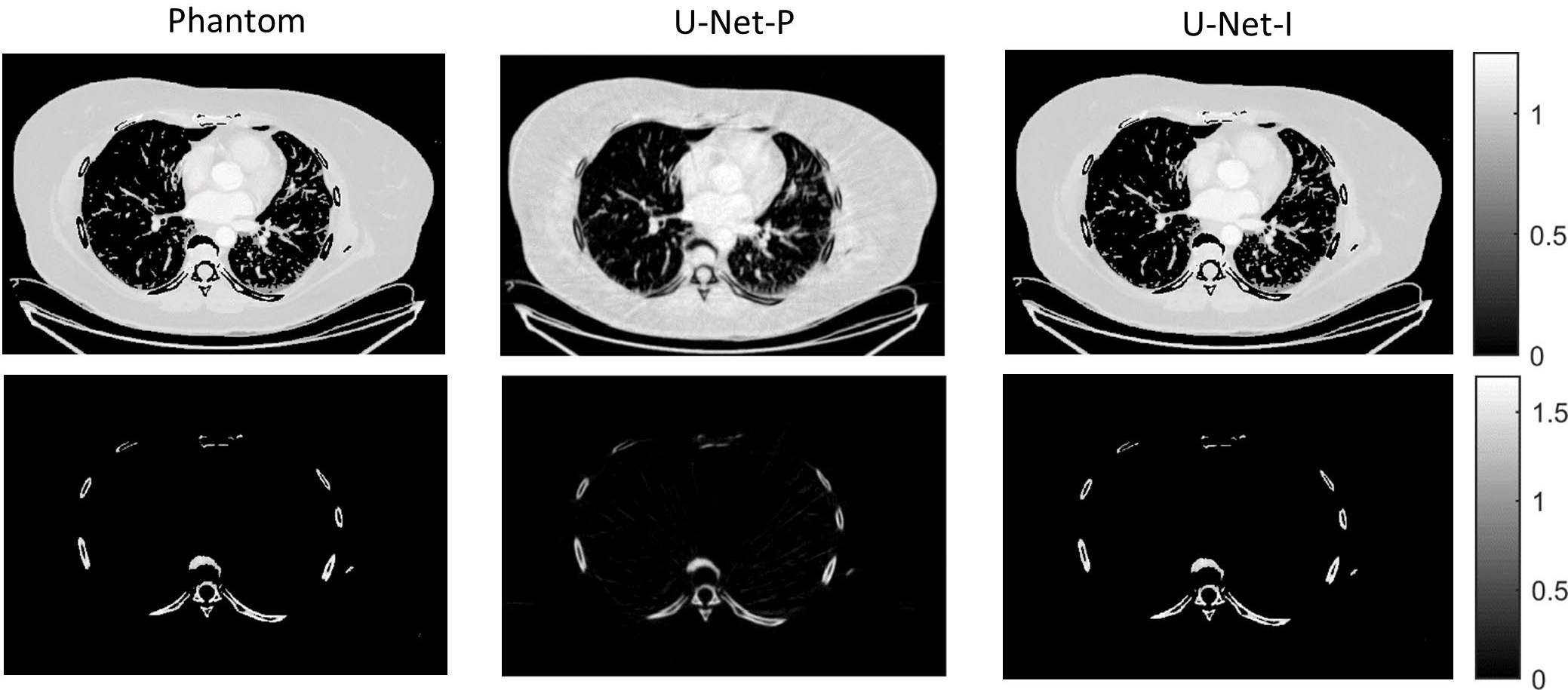
Figure 3: Material decomposition of simulated PCCT acquisitions of a patient phantom (left) with projection-based (middle) and image-based (right) U-Net CNN. The two materials of the decomposition are soft tissue (top row) and bone (bottom row). Figure adapted from [129] [129] and distributed under a Creative Commons Attribution 4.0 License, see https://creativecommons.org/licenses/by/4.0/.

The different approaches for material decomposition differ on many levels, from computational cost to the accuracy of the decomposed images. For example, [129] [129] compared projection-based and image-based algorithms using variational approaches and machine learning. They observed the best image quality with an image-based material decomposition approach, as illustrated in Fig. 3. However, the recent Grand Challenge on Deep-Learning spectral Computed Tomography [174] demonstrated that many different approaches are still under investigation. Nine out of the ten best scorers used machine learning and most combined it with a model of the DECT acquisition. The development of such algorithms in clinical scanners will depend on both their practicality, e.g. the computational time, and the accuracy of the material decomposition of real data.

V Data Pre-processing and Image Post-processing

CT technology has been the front-line imaging tool in emergency rooms due to its fast, non-invasive, and high-resolution features, with millions of scans performed annually worldwide. However, due to the increased cancer incidence from radiation exposure, “as low as reasonably achievable” is the central principle to follow in radiology practice. Recent advances in CT technology and deep learning techniques have led to great developments in reducing radiation doses in CT scans [175]. For example, aided by deep learning techniques, much progress has been made in low-dose or few-view CT reconstruction without sacrificing significant image quality. Furthermore, the use of DECT technology allows further cuts in radiation dose by replacing previous non-contrast CT scans with virtual unenhanced images in clinical practice [176].

While many prior-regularized iterative reconstruction techniques described in Section III inherently suppress noise and artifact, network-based post-processing techniques are also popular for removing noise and artifacts from already reconstructed low-dose spectral images and are covered here. Moreover, PCCT with PCD is widely viewed as a comprehensive upgrade to DECT since it produces less noise, better spectral separation, and higher spatial resolution while requiring less radiation dose [30, 29]. However, the PCD often experiences increased nonuniformity and spectral distortion due to charge-sharing and pulse pile-up effects compared to the traditional EID, and the correction of these imperfections in PCD images is included here. Finally, we also review deep learning techniques that enhance clinical diagnosis with spectral CT, which includes virtual monoenergetic image synthesis, virtual noncontrast image generation, iodine dose reduction, virtual calcium suppression, and other applications. The overview of this section is summarized in Fig. 4.

Figure 4: Overview of sub-topics in Section V. The data pre-processing section covers deep correction methods for spectral distortion (e.g., falsely increased counts in the low energy bin due to the charge sharing effect, and non-linear responses due to the pulse pileup effect) and non-uniformity in PCD projection images. The image post-processing sections discuss deep post-processing methods to enhance DECT and PCCT imaging and their impacts on clinical diagnosis.

V-A PCCT Data Pre-processing

PCD offer much smaller pixel size compared to EIDs and also possess energy discrimination ability that can greatly enhance CT imaging with significantly higher spatial and spectral resolution. However, PCD measurements are often distorted by undesired charge sharing and pulse pileup effects, which can limit the accuracy of attenuation values and material decomposition. Since accurately modeling these effects is highly complex, deep learning methods are being actively explored for distortion correction in a data driven manner. The initial trial is introduced in [144] [144] where a simple fully-connected NN with two hidden layers of five neurons each was adopted mainly for charge sharing correction. Later the same network structure but with more neurons was used by [177] [177] to compensate pulse pileup distortion, and similarly in [178, 179] for spectral distortion correction. A large CNN model was first introduced in [180] [180] to leverage inter-pixel information for both corrections of charge sharing and pulse pileup effects. The model included a dedicated generator with a pixel-wise fully-connected sub-network for intra-pixel distortion caused by pulse pileup and a convolutional sub-network for inter-pixel cross-talk correction, and was trained using the WGAN framework for spectral correction. More recently, [181] [181] used multi-energy CT scans with an EID to calibrate the PCD spectral distortion, and adopted a U-Net to map the distorted PCD projections into monochromatic projections generated by multi-energy CT scans after material decomposition. [182] [182] introduced CNN-LSTM to correct pulse pileup distortion in X-ray source spectrum measurements, while [183] [183] used a spatial-temporal CNN for charge sharing compensation.

There are also several interesting studies on artifact correction for PCCT using deep learning methods. [184] [184] utilized a U-Net for scatter correction in the sinogram domain to compensate for the Moiré artifacts caused by coarse anti-scatter grids relative to the small detector pixel size, resulting in improved image quality and HU value accuracy. Due to the complexity of PCD, their pixels tend to suffer more nonuniformity due to detector imperfections compared to EID, making the ring artifact issues more prominent in PCCT. To address this issue, [185] [185] trained a U-Net with the perceptual loss for the correction of ring artifacts caused by pixel nonuniformity [186], while [187] [187] used two U-Nets in both projection domain and image domain for ring artifacts removal.

V-B Image Post-processing

V-B1 Image Denoising

In CT imaging, it is important to limit the radiation dose to patients, but reducing the dose often gives rise to image noise, which can strain radiologists’ interpretation. To address this issue, various image denoising methods have been developed that aim to recover a clean version $\bm{\mu}^{\star}$ from a noisy image $\bm{\mu}^{0}$ by leveraging prior knowledge $R$ of the image to maintain sufficient image quality for clinical evaluation,

$$\bm{\mu}^{\star}=\operatornamewithlimits{arg\,min}_{\bm{\mu}}\left\|\bm{\mu}-\bm{\mu}^{0}\right\|_{2}^{2}+\beta R(\bm{\mu}).$$ (47)

The development of CT noise reduction techniques has a long history with its root dating back shortly after the invention of CT. While our focus is on deep learning and spectral CT, it is important to briefly cover classic post-processing denoising techniques and deep learning techniques for single energy CT, as they can still be applied to spectral CT in a channel-by-channel manner. We will then dive into recent trends of self-supervised learning deep denoising methods, as well as deep methods that incorporate the correlations between energy channels.

Spatial filtering methods leverage the statistical nature of noise fluctuations and are achieved through local averaging or nonlocal averaging means [188, 189, 190]; optimization-based denoising methods, on the other hand, incorporate image model preassumptions such as domain sparsity, piecewise linearity, or gradient smoothness as regularization. Some well-known methods in this category include TV [191], DL [192, 72], wavelet based denoising [193], BM3D [194], and others. A good discussion of these classic denoising techniques is provided by [195] in their review paper [195]. Different from the explicitly defined prior knowledge in traditional methods, the development of deep learning techniques, particularly CNN, provides a data-driven approach to learn the implicit distribution knowledge from large amounts of images, offering a one-step solution to the denoising problem (Eq. (47)), i.e.,

$$\bm{\mu}^{\star}=\bm{\mathcal{F}}_{\bm{\theta}^{\star}}\left(\bm{\mu}^{0}\right),$$ (48)

where $\bm{\mathcal{F}}_{\bm{\theta}^{\star}}$ denotes the network function with optimized parameters $\bm{\theta}^{\star}$ after training. Since they are way more powerful than the traditional methods, deep methods will soon dominate the research field of CT image denoising. Initially, these methods were primarily trained in a supervised fashion using paired noisy and clean images, as generally depicted by Eq. (49), and the successful examples include REDCNN [196], wavelet network [197] and stacked competitive network [198].

$$\bm{\theta}^{\star}=\operatornamewithlimits{arg\,min}_{\bm{\theta}}\mathbb{E}\left[\mathcal{L}\left(\bm{\mathcal{F}}_{\bm{\theta}}\left(\bm{\mu}^{0}\right),\bm{\mu}^{1}\right)\right],$$ (49)

where $\mathcal{L}(\cdot,\cdot)$ denotes a general loss function for network training, $\bm{\mu}^{1}$ is the clean image corresponding to the noisy one $\bm{\mu}^{0}$ and the expectation is taken over pairs $(\bm{\mu}^{0},\bm{\mu}^{1})$ from the training dataset. Following the idea, various network structures and loss functions have been explored. Representative network structures include U-Net [199, 200, 201], DenseNet [202], GAN [203, 204, 205, 206], ResNet [207, 208], Residual dense network [209], Quadratic neural network [210], transformer [211], diffusion model [212], and more. Commonly used loss functions include MSE, MAE, structural similarity index [213, 214, 215], adversarial loss [216, 203], TV loss [217, 218], perceptual loss [219, 203], edge incoherence [220], identity loss [221, 222, 206], projection loss [215], and more. For more detailed information, we refer readers to the latest two review papers on low-dose CT denoising [223, 224].

The issue of missing paired labels was soon realized when researchers attempted to apply supervised methods in practice. To address this, a number of unsupervised or self-supervised methods have been proposed. For instance, cycle-GAN based techniques are able to utilize unpaired data for training by promoting cycle consistency between domains [206, 222, 225, 205]. However, these GAN-based methods have been criticized for potentially generating erroneous structures. Poisson Unbiased Risk Estimator (PURE) and Weighted Stein’s Unbiased Risk Estimator (WSURE) are alternative methods that convert the supervised MSE loss calculation into a form that only relies on the noisy input, the network output, and its divergence [226]. This approach forms an unsupervised training framework where the divergence term is approximated using Monte-Carlo perturbation method [227]. Noise2Noise is another method that enables us to train the network with paired noise-noise images which are equivalent to being trained with original noise-clean pairs,

$$\bm{\theta}^{\star}=\operatornamewithlimits{arg\,min}_{\bm{\theta}}\mathbb{E}\left[\left\|\bm{\mathcal{F}}_{\bm{\theta}}\left(\bm{\mu}^{0}\right)-\bm{\mu}^{1}\right\|_{2}^{2}\right],$$ (50)

where $\bm{\mu}^{0}$ and $\bm{\mu}^{1}$ are different noisy realizations of the same image, e.g., two independent CT scans of the same object. Building on this idea, several recent variant methods have been developed for self-supervised low-dose CT denoising by generating noisy pairs via various approaches [228, 229, 230, 231, 232, 233, 234, 235, 236]. For instance, Noise2Inverse proposes to partition projection data into several sets and enforcing consistency between corresponding reconstructions [234], while Noise2Context promotes similarity between adjacent CT slices in 3D thin-layer CT [232]; Half2Half adopts the thinning technique [237] to split a full dose real CT scan into two pseudo half dose scans [230].

Spectral CT powerfully extends the conventional single energy CT by introducing an extra energy dimension. However, the splitting of photons into different energy bins increases the noise level of the projection at each bin compared to conventional CT with the same overall radiation dose. Therefore, to achieve optimal denoising performance for spectral CT, it is necessary to leverage inter-bin information, similar to the approach taken in learned synergistic reconstruction (Section III-E), as described below,

$$[\bm{\mu}_{1}^{\star},\dots,\bm{\mu}_{K}^{\star}]=\bm{\mathcal{F}}_{\bm{\theta}^{\star}}\left(\bm{\mu}_{1}^{0},\dots,\bm{\mu}_{K}^{0}\right)\,.$$ (51)

Several recent papers have explored this direction. ULTRA [238] incorporates an $\ell^{p}$-norm and anisotropic total variation loss to train a residual U-Net with multichannel inputs from PCCT scans. Noise2Sim [235] constructs noisy pairs using the Noise2Noise principle and replaces each pixel from the original noisy image with one of its $k$-nearest pixels searched from the spatial dimension (including adjacent slices) and measured by non-local means. The multichannel image is fed to the network as a whole, and its value from different bins can be constructed independently to fully leverage the self-similarities within the spectral CT scans. By this means, comparable or even better performance has been demonstrated on experimental PCCT scans against the supervised learning methods. S2MS [231] proposes another interesting approach to leverage the inter-channel information by converting the linear attenuation map from each channel to a channel-independent density map, which forms different noisy realizations of the density images from multiple channels. Promising results from this self-supervised learning idea are demonstrated on a simulation study.

Besides developing various deep denoising methods, researchers have also investigated the effects of noise reduction on the downstream tasks [239, 238]. For example, [239] [239] compared the material decomposition results of multi-bin PCCT images before and after denoising with BM3D and Noise2Sim through phantom studies. They found that image denoising improves the accuracy of material concentration quantification results, but not material classification results. In the clinical domain, there are several FDA-approved deep denoising methods from multiple vendors (e.g., the TrueFidelity from GE Healthcare, the Advanced Intelligent Clear-IQ Engine (AiCE) from Canon, PixelShine from Algomedica, ClariCT.AI from ClariPI Inc., etc), and numerous studies have been performed to investigate their impacts on clinical significance. For ease of notation, we use DLIR to refer specially to these FDA-approved methods in clinical applications. [240] [240] showed that with DLIR, the radiation dose of whole-body CT can be reduced by up to 75% while maintaining similar image quality and lesion detection rate compared to standard-dose CT reconstruction with iterative reconstruction through a study cohort of 59 patients. This conclusion is also supported in other studies where DLIR and iterative reconstruction of the same patient scans are compared, showing that DLIR provides significantly preferred image quality and reduced noise [241, 242].

For the diagnosis with DECT, the pancreatic cancer diagnostic acceptability and conspicuity can be significantly improved, and the use of DLIR reduces the variation in iodine concentration values while maintaining their accuracy [243]. [244] [244] suggests similar results in terms of iodine concentration quantification through both phantom and clinical studies. The stability of iodine quantification accuracy with DLIR has also been investigated in the context of radiation dose variation. For example, [245] [245] found that the accuracy is not affected by the radiation dose when the dose index is greater than 12.3 mGy. For a more detailed assessment of DLIR in clinical practice, a recent review paper by [246] [246] provides a good starting point. It is also worth noting that the aforementioned studies with PCCT [239] and DECT [244] lead to different conclusions about the impacts of denoising on iodine/material concentration quantification, which could be attributed to the different energy discrimination mechanisms between PCCT and DECT, as the number of energy bins and spectral separation can significantly influence the accuracy and stability of material decomposition performance [30].

V-B2 Artifacts Correction

Besides noise, image artifact is another factor that affects the quality of CT image for diagnostic evaluation. Few-view or limited-angle reconstruction is an effective method to reduce the radiation dose, but it can introduce globally distributed artifacts that are difficult to remove. To be concise and avoid overlap with Section III, here we only cover recent progress on post-processing-based artifact reduction approaches via deep learning for spectral CT. The networks are often trained in a supervised manner for this application and directly applied to FBP reconstructions to remove artifacts, which can be similarly described as Eq. (49) and Eq. (48) with $\bm{\mu}^{0}$ and $\bm{\mu}^{1}$ being few-view/limited-angle reconstruction and full-view/full-angle reconstruction respectively. For example, to reduce few-view reconstruction artifacts and accelerate reconstruction for scans at multiple energy points (i.e., 32 channels), [247] [247] proposed a U-Net-based approach that maps few-view FBP reconstruction images to computationally intensive full-view iterative reconstruction images with TV regularization. The 32-channel FBP images were fed to the network simultaneously and transformed to high-quality 32-channel reconstructions in one step, majorly reducing the computational cost. More recently, [248] [248] developed a multi-level wavelet convolutional neural network, using a U-Net architecture with the wavelet transform as the down-sampling/up-sampling operations, that effectively captures and removes globally distributed few-view artifacts. The network simultaneously processes multi-channel images to leverage inter-channel information, and demonstrates promising results both numerically and experimentally with an edged silicon strip PCD. To address limited-angle artifacts for cone beam DECT, [249] [249] proposed the TIME-Net, which utilizes a transformer module with global attention. In addition, the two complementary limited-angle scans at two energies are fused together to form a prior reconstruction, then the features extracted from the prior reconstruction, high-energy reconstruction, and low-energy reconstruction are fused in latent space to leverage inter-channel information with the network.

In dual-source DECT scanners, the high-energy imaging chain (i.e., tube B with a tin filter, typically at 140 keV) often has a restricted FOV (e.g., 33cm) due to physical constraints compared to the other chain (e.g., 50cm for tube A), which can be problematic for larger patients and affect diagnosis. To outpaint the missing regions and match the size of normal FOV, [250] [250] proposed a self-supervised method that maps the low-energy image to the high-energy image with a loss function only focusing on image values within the restricted FOV. The outpainting is then automatically completed leveraging the shift-invariant nature of CNN. Similarly, [251] [251] proposed a method for FOV extension that involves feeding both the high-energy image and the low-energy image in the network, along with a high-energy estimation from the low-energy image via a piecewise-linear transfer function. The trained network was applied to patient data for renal lesion evaluation and showed reliable results in terms of HU value and lesion classification accuracy in the extended regions.

V-C Image Generation for Clinical Applications

With the recent development of DECT and PCCT techniques, spectral imaging is reshaping the clinical utilization of CT. These techniques enable the generation of multiple types of images that enhance diagnosis and improve disease management, such as VMI, virtual unenhanced images, bone suppression images, and material decomposition maps. A good number of research studies have been performed in these areas using deep learning approaches.

V-C1 Single-Energy to Dual-energy Mapping

Despite the great possibilities offered by DECT and PCCT, their accessibility remains limited in comparison to conventional single-energy CT, largely due to the high cost involved. To bridge the gap, [252] [252] successfully demonstrated the feasibility of using deep learning to predict high-energy CT images from given low-energy CT images in a retrospective study. Shortly, [253] [253] proposed a material decomposition CNN capable of generating high-quality DECT images from a low-energy scan combined with a single view high-energy projection, leveraging the anatomical consistency and energy-domain correlation between two energy images in DECT. The feasibility of this method has been validated with patient studies, showing great potential for simplifying DECT hardware and reducing radiation exposure during DECT scans.

V-C2 Virtual Monochromatic Image

VMI are widely used as the basis for routine diagnosis due to their ability to reduce beam-hardening and metal artifacts, and enhance iodine conspicuity. They are obtained by linearly combining the basis material volume fraction maps [115, 254] obtained after material decomposition, as described by the material decomposition model in Section IV. To enhance readability and clarity, Eq. (36), which outlines this model, is replicated here in a spatially discrete form:

$$\bm{\mu}(E)=\sum_{m=1}^{M}{f_{m}(E)\bm{x}_{m}},$$ (52)

where $\bm{x}_{m}$ denotes the volume fraction map of the $m$^th material basis, $f_{m}(E)$ stands for the linear attenuation coefficient of the corresponding material at energy $E$, and $M$ is the total number of material basis. However, the synthesis of VMI relies on material decomposition results and is therefore limited to DECT and PCCT, which may not be available in less developed areas. Similar to section V-C1, a number of approaches have been explored to directly synthesize the VMI from single-energy CT scans. [255] [255] first used a modified ResNet for VMI generation from single polychromatic CT scans, then developed a sinogram domain method [256] synthesizing VMI with a fully-connected NN for virtual monochromatic energy sinogram prediction from single polychromatic measurements. [257] [257] employed a GAN to generate VMI from equivalent keV-CT images, while [258] [258] used a U-Net for a similar purpose in imaging of head and neck cancers. More interestingly, [259] [259] found that using VMI synthesized from single-energy CT images for pulmonary embolism classification provides better performance compared to working directly on the original single-energy images.

On the other hand, VMI synthesis is a downstream task after image reconstruction and material decomposition, during which deep denoising plays a role and potentially affects VMI quality in clinical practice. Extensive studies have investigated this effect through quantitative assessment and/or subjective reader studies. [245] [245] examined VMI CT number accuracy at various radiation doses, finding that accuracy remains unaffected except at extremely low radiation doses (6.3 mGy). [260] [260] compared VMI from DLIR with routine baselines from hybrid iterative reconstruction for contrast-enhanced abdomeninal DECT imaging, concluding that vessel and lesion conspicuity of VMI and iodine density images are improved with DLIR. [261] [261] reached a similar conclusion, and particularly they found that 40 keV VMI from DLIR poses better CNR and similar or improved image quality compared to 50 keV VMI from hybrid iterative reconstruction, suggesting that 40 keV VMI with DLIR could be a new standard for routine low-keV VMI reconstruction. The study for carotid DECT angiography by [262] [262] also supports the conclusion that DLIR improves the image quality and diagnostic performance of VMI compared to hybrid iterative reconstruction. This superiority is further confirmed in DECT angiography with reduced iodine dose (200 mgI/kg) in terms of image quality and arterial depiction by [243] [243]. Additionally, the effect of direct denoising on VMI has been investigated. In a study of [263] [263] the post-processed VMI using ClariCT.AI (a FDA-approved vendor-agnostic imaging denoising software) is compared with original standard VMI in the assessment of hypoenhancing hepatic metastasis. The results suggest denoising leads to better image quality and lesion detectability. A similar conclusion was achieved by [264] [264] with the same post-denoising method for the evaluation of hypervascular liver lesions.

V-C3 Contrast Agent Dose Reduction

Iodine-enhanced CT is essential for diagnosing various diseases. However, iodine-based contrast media can cause significant side effects, including allergic reactions in certain patients, and dose-dependent kidney injury and thyroid dysfunction. To investigate the possibility of reducing iodine administration dose while maintaining diagnostic accuracy, [265] [265] trained a GAN to selectively enhance iodine contrast. They ultimately achieved a 50% contrast dose saving ratio, confirmed by a visual Turing test involving three radiologists assessing pathological consistency. [266] [266] explored the potential of leveraging vendor DLIR for simultaneous iodine and radiation dose reduction in thoraco-abdomino-pelvic DECT imaging. They compared the 40 keV VMI from DLIR of double low-dose (50% iodine, 50% radiation) scans with VMI from the hybrid iterative reconstruction of standard dose scans. The diagnostic image quality was achieved in 95% of participants in the double low-dose group, suggesting the feasibility of maintaining diagnostic quality at half doses of radiation and iodine using DLIR.

V-C4 Others

Several other intriguing deep post-processing techniques for spectral CT include virtual non-contrast image synthesis, virtual non-calcium image synthesis, and spectral CT-based thermometry. Virtual non-contrast images can replace non-contrast scans in a DECT scanning protocol, thus saving radiation dose. However, pure physics-based two-measurement material decomposition algorithms exhibit limited accuracy and stability in the presence of three materials. [267] [267] employed a CNN to leverage the anatomic information, bridging the gap between material decomposition-derived virtual non-contrast images and the real non-contrast images to generate higher fidelity images.

Virtual non-calcium images are useful for visualizing bone marrow, osteolytic lesions, and even the diagnosis of multiple myeloma [268, 269]. Like virtual non-contrast images, they also suffer from excessive noise and artifacts resulting from material decomposition. [137] [137] proposed a custom dual-task CNN that directly maps the input of spectral CT images to material type maps and corresponding mass density maps. The experimental results demonstrate significantly reduced noise and artifacts in virtual non-calcium images and great visibility of bone marrow lesions.

CT-based thermometry provides a non-invasive method for estimating temperature inside the human body by monitoring the attenuation value changes associated with temperature-dependent radiodensity. [270] [270] explored the potential of improving temperature sensitivity with VMI from DLIR of DECT scans compared to conventional single-energy CT images. Their results show that VMI significantly enhances temperature sensitivity for different materials, particularly for bone with a boost of 211%. The application of DLIR and hybrid iterative reconstruction has no effect on temperature measurement, suggesting the great potential for dose reduction with deep learning techniques. More recently, [271] [271] incorporated an advanced PCD with 4 energy bin measurements for robust material decomposition and a fully-connected NN for temperature prediction. They observed a non-linear relationship between thermal sensitivity and the concentration of CaCl₂ solution in the experiment, achieving final thermometry accuracies of $3.97^{\circ}$C and $1.8^{\circ}$C for 300 mmol/L CaCl₂ solution and a milk-based protein shake, respectively.

VI Perspectives

Advances in spectral CT is a major frontier of the medical CT field, which combines cutting-edge hardware for photon-counting detection and AI-empowered software for deep learning-based reconstruction. As we have reviewed above, photon-counting spectral CT promises to significantly improve the medical CT performance in terms of spatial resolution, spectral resolution, tissue contrast, and dose efficiency. The distinguished capability of photon-counting CT in material decomposition is clinically attractive to perform novel multi-contrast-enhanced studies and boost CT, not only in anatomical imaging but also functional or even cellular imaging tasks. All of these can be implemented using machine learning methods or coupled with machine learning methods. Most of such machine learning methods are deep neural networks, involving each key step in the whole imaging workflow.

Looking ahead, the convergence of photon-counting and deep-learning techniques will surely establish spectral CT as the new standard of medical CT. To realize the huge potential of photon-counting spectral CT, there remain challenges to be addressed before task-specific methods and protocols can be successfully translated into clinical practice. These challenges include but are not limited to the following aspects.

Direct Reconstruction

Deep NN have been explored to reconstruct images from sinograms in a number of studies. In this approach, a neural network is trained on a large set of sinogram-image pairs until the network predicts realistic reconstructed images. Here, the NN learns to reconstruct the image and at the same time to reduce noise and to incorporate any other corrections desirable for reconstruction. Early methods developed for tomographic reconstruction using deep networks include AUTOMAP [272] for MR reconstruction as well as LEARN [273] and iCT [274] for CT reconstruction. To tackle the computational complexity, more sophisticated and efficient networks were developed [275, 276, 277, 278].

Direct reconstruction techniques may be extended to multichannel reconstruction including photon-counting spectral CT reconstruction. One possible way would be to have multi-channel networks incorporating data in multiple energy bins or an ensemble of networks with weight sharing for each energy. Importantly, correlations among these data in these channels should be utilized; for example, as a term in the loss function.

Locally linear embedding Motion Correction

The much-reduced pixel size of PCD enables CT imaging at ultra-high resolution, which is one major advantage of PCCT over traditional EID-based CT and critical to resolve anatomical and pathologic details, such as cochlear features, lung nodules, and coronary plaques. As resolution drastically improves, the sensitivity to patient motion and geometric misalignment becomes high and can be the limiting factor of image resolution. This increased sensitivity also challenges the assumption of smooth patient movement across views [279, 280, 281].

To address the issue, [282] [282] developed a rigid patient motion compensation method for high-resolution helical PCCT based on LLE. Their method is in a coarse-to-fine searching framework to boost efficiency, along with several accuracy improving steps masking bad pixel, unreliable volume and patient bed respectively. The method was evaluated on patient wrist scans in a clinical trial, revealing fine bony structures previously hidden by motion blur, as shown in Fig. 5. Subsequently, [283] [283] proposed a unified reference-free all-in-one motion correction method for robotic CT with arbitrary scanning trajectories using a nine-degree-of-freedom model, which is capable of addressing rigid patient motion, system misalignment, and coordination errors simultaneously. The effectiveness of the method has been verified on experimental robotic-arm-based PCCT scans of a sacrificed mouse demonstrating a great resolution boost and artifacts reduction.

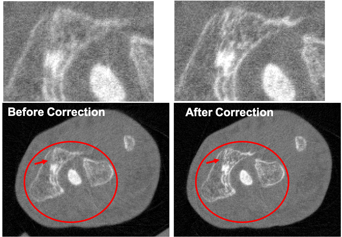
Figure 5: High-resolution PCCT scan of a patient wrist from a clinical trial (90 $\mu$m voxel) before and after motion correction (Adapted from [282] [282] with permission).

Diffusion Models

As a score-matching-based generative approach, the DM have recently drawn a major attention of the community as they effectively compete or even outperform GAN for image generation and other tasks [284], and have been broadly adapted for medical imaging [285], including PCCT image generation [286]. They involve gradually degrading a sample of interest (i.e., an image) with subtle Gaussian noise until the sample becomes a random Gaussian field, learning the noising process in terms of a score function, and then, by inversion from a Gaussian noise realization, generate a meaningful sample [287]. Specifically, the inverse process uses the gradient of the log-density of the prior (the score) which is approximated with a NN trained for score matching, and generates an image according to the a-priori probability distribution of the training dataset.

DM can be used to solve inverse problems by adding a data fidelity gradient descent step in the inverse diffusion, or by using the pseudo a-posteriori probability distribution conditioned to the observed data, which work in an unsupervised manner. These methods have been used in various inverse problems such as deblurring on RGB multichannel images [288]. Moreover, the DM are independent of the measurement model, and the same approaches can be used in multi-energy spectral CT reconstruction or one-step material decomposition under different imaging geometries and sampling conditions. Recently,

Hardware Refinement

Over the past years, photon-counting detectors have been greatly refined. There are more efforts on CZT detectors, but deep-silicon detectors are also of great interest. While CZT detectors and alike are more compact, the silicon technology is more mature, reliable and cost-effective with the potential to give more quantitative spectral imaging results. A detailed comparison is yet to be seen. Since the photon-counting detector pitches are substantially smaller than that of the energy-integrating detectors, the spatial resolution of CT images can be accordingly improved, coupled with a reduced X-ray source focal spot. However, a small focal spot usually means a low X-ray flux. Hence, the balance must be made between image resolution, noise and imaging speed. It is underlined that while the hardware refinement in either detectors or sources is important, this kind of research will be more often performed by leading companies than academic groups. Since this review is more focused on computational aspects of spectral CT, in the following we discuss more AI-related challenges.

Big Data Construction

It is well known that big data is a prerequisite for data-driven research. Clearly, it is not easy to have big PCCT data for several reasons, including limited accessibility to PCCT scans, patient privacy, industrial confidentiality, and so on. We believe that this issue must be addressed using simulation tools, and ideally done in a healthcare metaverse. Such an idea was discussed as the first use case in a recent perspective article [289]. Along that direction, virtual twins of physical PCCT scanner models can scan patient avatars to produce simulated data. Along a complementary direction, a limited number of real PCCT scans can be used to train a generative model for realistic image augmentation. For example, it was recently shown that the diffusion model can be used to synthesize realistic data with suppressed privacy leakage [290]. This will facilitate federated learning at the level of datasets.

AI model Development

When sufficiently informative PCCT data are available, more advanced AI models should be developed to address current weaknesses of deep reconstruction networks in the CT field. The well-known problems of deep networks include stability, generalizability, uncertainty, interpretability, fairness, and more. As briefly mentioned in our review, a unique opportunity in deep learning-based PCCT imaging is raw data correction for charge-sharing, pile-up and other effects. These effects are very complicated, nonlinear and stochastic, but deep learning-based solutions are few and there will be more in the future. Furthermore, large models are gaining great attention, with ChatGPT as a precursor of the next generation of AI methods, i.e., as the first step into the future of AGI. It is believed that large models, multi-modal large models in particular, will further improve the PCCT performance.

High-performance and High-efficiency Computing

Deep learning with large models takes computational resources. Parallel/cloud computing, model distillation and hybrid (combination of classic and deep learning) reconstruction methods can be synergistic to develop practical PCCT methods. Special hardware such as FPGAs [291] could be adapted in PCCT tasks for imaging speed and energy efficiency.

Clinical Translation

The development of accurate and robust PCCT methods should lead to diverse clinical applications, from screening and diagnosis to treatment planning and prognosis. PCCT can be also used to guide minimally invasive procedures, such as biopsy and ablation, by providing real-time information over a region of interest [292]. The integration of PCCT (and DECT) with other imaging modalities, such as MRI and PET, would be beneficial as well, leading to a better understanding of anatomical forms and pathological functions.

Hybrid PET/CT Spectral Imaging

The integration of spectral CT with PET has the potential to open novel clinical applications. However, such an integrated system either requires a costly hardware upgrade or is associated with increased radiation exposure. Most existing spectral CT imaging methods are based on a single modality that uses X-rays. Alternatively, it is possible to explore a combination of X-ray and $\gamma$-ray for spectral imaging [293]. The concept of this PET-enabled spectral CT method exploits a standard time-of-flight PET emission scan to derive high-energy $\gamma$-ray CT attenuation images and combines the images with low-energy X-ray CT images to form dual-energy or multi-energy imaging. This method has the potential to make spectral CT imaging more readily available on clinical PET/CT scanners. The enabling algorithm of this hybrid spectral imaging method is the reconstruction of $\gamma$-ray attenuation images from PET emission data using the maximum-likelihood attenuation and activity algorithm [294, 293]. While the counting statistics of PET emission data are relatively low, machine learning-based approaches have been developed to further improve image reconstruction, for example, using the kernel method alone [293, 295] or in combination with deep neural networks [296, 297, 298]. These reconstruction approaches are directly based on single subjects without requiring pretraining from a large number of datasets. Alternatively, many other big data-based deep learning techniques that are described in Section III, Section IV, and Section V may be applied to the development of hybrid PET/CT spectral imaging.

VII Conclusion

In conclusion, this review has systematically reviewed spectral CT with an emphasis on photon-counting and deep learning techniques. This field has evolved from traditional DECT with an established status in medical imaging to contemporary PCCT with promising results and new utilities. Several remaining challenges have been discussed. The future of this technology looks exciting, with numerous opportunities for us to explore so that our imaging dreams can be turned into reality.

References

- [1] Katsuyuki Taguchi and Jan S Iwanczyk “Vision 20/20: single photon counting x-ray detectors in medical imaging” In Medical physics 40.10 Wiley Online Library, 2013, pp. 100901
- [2] Katsuyuki Taguchi, Rafael Ballabriga, Michael Campbell and Dimitra G Darambara “Photon counting detector computed tomography” In IEEE Transactions on Radiation and Plasma Medical Sciences 6.1 IEEE, 2021, pp. 1–4
- [3] Katsuyuki Taguchi, Christoph Polster, W Paul Segars, Nafi Aygun and Karl Stierstorfer “Model-based pulse pileup and charge sharing compensation for photon counting detectors: A simulation study” In Medical physics 49.8 Wiley Online Library, 2022, pp. 5038–5051
- [4] W Yang Tai, Donghyeon Lee, Xiaohui Zhan, Katsuyuki Taguchi and Wojciech Zbijewski “Effects of bowtie scatter on material decomposition in photon-counting CT” In Medical Imaging 2023: Physics of Medical Imaging 12463, 2023, pp. 26–31 SPIE
- [5] Geert Litjens, Thijs Kooi, Babak Ehteshami Bejnordi, Arnaud Arindra Adiyoso Setio, Francesco Ciompi, Mohsen Ghafoorian, Jeroen Awm Van Der Laak, Bram Van Ginneken and Clara I Sánchez “A survey on deep learning in medical image analysis” In Medical image analysis 42 Elsevier, 2017, pp. 60–88
- [6] Berkman Sahiner, Aria Pezeshk, Lubomir M Hadjiiski, Xiaosong Wang, Karen Drukker, Kenny H Cha, Ronald M Summers and Maryellen L Giger “Deep learning in medical imaging and radiation therapy” In Medical physics 46.1 Wiley Online Library, 2019, pp. e1–e36
- [7] Inês Domingues, Gisèle Pereira, Pedro Martins, Hugo Duarte, João Santos and Pedro Henriques Abreu “Using deep learning techniques in medical imaging: a systematic review of applications on CT and PET” In Artificial Intelligence Review 53 Springer, 2020, pp. 4093–4160
- [8] HARRY K. GENANT and DOUGLAS BOYD “Quantitative Bone Mineral Analysis Using Dual Energy Computed Tomography” In Investigative Radiology 12.6, 1977, pp. 545–551
- [9] Sharon Z Adam, Aviad Rabinowich, Rivka Kessner and Arye Blachar “Spectral CT of the abdomen: Where are we now?” In Insights into Imaging 12.1, 2021, pp. 138
- [10] Reza Forghani, Bruno De Man and Rajiv Gupta “Dual-energy computed tomography: Physical principles, approaches to scanning, usage, and implementation: Part 1” In Neuroimaging Clin. N. Am. 27.3, 2017, pp. 371–384
- [11] Juergen Fornaro, Sebastian Leschka, Dennis Hibbeln, Anthony Butler, Nigel Anderson, Gregor Pache, Hans Scheffel, Simon Wildermuth, Hatem Alkadhi and Paul Stolzmann “Dual- and multi-energy CT: approach to functional imaging” In Insights Imaging 2.2, 2011, pp. 149–159
- [12] Thorsten R C Johnson “Dual-energy CT: general principles” In AJR Am. J. Roentgenol. 199.5 Suppl American Roentgen Ray Society, 2012, pp. S3–8
- [13] Bernhard Krauss “Dual-energy computed tomography: Technology and challenges” In Radiol. Clin. North Am. 56.4, 2018, pp. 497–506
- [14] Cynthia H McCollough, Shuai Leng, Lifeng Yu and Joel G Fletcher “Dual- and multi-energy CT: Principles, technical approaches, and clinical applications” In Radiology 276.3 Radiological Society of North America (RSNA), 2015, pp. 637–653
- [15] Prabhakar Rajiah, Suhny Abbara and Sandra Simon Halliburton “Spectral detector CT for cardiovascular applications” In Diagn. Interv. Radiol. 23.3, 2017, pp. 187–193
- [16] “Dual energy CT in clinical practice”, Diagnostic Imaging Berlin, Germany: Springer, 2010
- [17] Alec J Megibow, Avinash Kambadakone and Lakshmi Ananthakrishnan “Dual-energy computed tomography: Image acquisition, processing, and workflow” In Radiol. Clin. North Am. 56.4, 2018, pp. 507–520
- [18] Joël Greffier, Nicolas Villani, Didier Defez, Djamel Dabli and Salim Si-Mohamed “Spectral CT imaging: Technical principles of dual-energy CT and multi-energy photon-counting CT” In Diagn. Interv. Imaging Elsevier BV, 2022
- [19] Thomas G Flohr, Cynthia H McCollough, Herbert Bruder, Martin Petersilka, Klaus Gruber, Christoph Süss, Michael Grasruck, Karl Stierstorfer, Bernhard Krauss, Rainer Raupach, Andrew N Primak, Axel Küttner, Stefan Achenbach, Christoph Becker, Andreas Kopp and Bernd M Ohnesorge “First performance evaluation of a dual-source CT (DSCT) system” In Eur. Radiol. 16.2 Springer ScienceBusiness Media LLC, 2006, pp. 256–268
- [20] R. Carmi, G. Naveh and A. Altman “Material Separation with Dual-Layer CT” In IEEE Nuclear Science Symposium Conference Record IEEE, 2005
- [21] Alain Vlassenbroek “Dual Layer CT” In Dual Energy CT in Clinical Practice Springer Berlin Heidelberg, 2010, pp. 21–34
- [22] Philips “Advantages of a spectral detector-based CT system [White paper]”, https://www.philips.com/c-dam/b2bhc/master/landing-pages/spectral-ct/452299150831_WP_Advantages_of_spectral_detector_CT.pdf, 2013
- [23] Michal Gabbai, Isaac Leichter, Samuel Mahgerefteh and Jacob Sosna “Spectral material characterization with dual-energy CT: comparison of commercial and investigative technologies in phantoms” In Acta Radiol. 56.8 SAGE Publications, 2015, pp. 960–969
- [24] Liang Li, Tiao Zhao and Zhiqiang Chen “First Dual MeV Energy X-ray CT for Container Inspection: Design, Algorithm, and Preliminary Experimental Results” In IEEE Access 6, 2018, pp. 45534–45542
- [25] Kirsten Boedeker, Marette Hayes, Jian Zhou, Ruoqiao Zhang and Zhou Yu “Deep learning spectral CT-Faster, easier and more intelligent [White paper]”, Canon Medical Systems Corporation, https://global.medical.canon/products/computed-tomography/spectral, 2019
- [26] Yan Xi, Wenxiang Cong, Daniel Harrison and Ge Wang “Grating Oriented Line-Wise Filtration (GOLF) for Dual-Energy X-ray CT” In Sensing and Imaging 18.1, 2017
- [27] Hans Bornefalk and Mats Danielsson “Photon-counting spectral computed tomography using silicon strip detectors: a feasibility study” In Physics in Medicine & Biology 55.7, 2010, pp. 1999
- [28] R. Ballabriga, J. Alozy, M. Campbell, E. Frojdh, E.H.M. Heijne, T. Koenig, X. Llopart, J. Marchal, D. Pennicard, T. Poikela, L. Tlustos, P. Valerio, W. Wong and M. Zuber “Review of hybrid pixel detector readout ASICs for spectroscopic X-ray imaging” In Journal of Instrumentation 11.01, 2016, pp. P01007
- [29] Mats Danielsson, Mats Persson and Martin Sjölin “Photon-counting x-ray detectors for CT” In Physics in Medicine & Biology 66.3, 2021, pp. 03TR01
- [30] Martin J Willemink, Mats Persson, Amir Pourmorteza, Norbert J Pelc and Dominik Fleischmann “Photon-counting CT: Technical principles and clinical prospects” In Radiology 289.2 Radiological Society of North America (RSNA), 2018, pp. 293–312
- [31] Ehsan Samei, Jayasai Rajagopal and Elizabeth Jones “Hallway conversations in physics” In AJR Am. J. Roentgenol. 215.5 American Roentgen Ray Society, 2020, pp. W50–W52
- [32] Elisabeth Shanblatt, Jim O’Doherty, Martin Petersilka, Philipp Wolber, George Fung and Juan C. Ramirez-Giraldo “Whitepaper: The technology behind photon-counting CT”, Siemens Healthineers, https://www.siemens-healthineers.com/en-us/computed-tomography/technologies-and-innovations/photon-counting-ct, 2022
- [33] Tianye Niu, Xue Dong, Michael Petrongolo and Lei Zhu “Iterative image-domain decomposition for dual-energy CT” In Medical physics 41.4 Wiley Online Library, 2014, pp. 041901
- [34] Jian Feng, Haijun Yu, Shaoyu Wang and Fenglin Liu “Image-domain based material decomposition by multi-constraint optimization for spectral CT” In Ieee Access 8 IEEE, 2020, pp. 155450–155458
- [35] Polad M Shikhaliev “Projection x-ray imaging with photon energy weighting: experimental evaluation with a prototype detector” In Physics in Medicine & Biology 54.16 IOP Publishing, 2009, pp. 4971
- [36] Simon R Arridge, Matthias J Ehrhardt and Kris Thielemans “(An overview of) Synergistic reconstruction for multimodality/multichannel imaging methods” In Philosophical Transactions of the Royal Society A 379.2200 The Royal Society Publishing, 2021, pp. 20200205
- [37] F. Natterer “The Mathematics of Computerized Tomography”, Classics in Applied Mathematics SIAM, 2001
- [38] R. Gordon, R. Bender and G.. Herman “Algebraic Reconstruction Techniques (ART) for Three-Dimensional Electron Microscopy and X-Ray Photography” In Journal of Theoretical Biology 29.3 Elsevier, 1970, pp. 471–481
- [39] Peter Gilbert “Iterative methods for the three-dimensional reconstruction of an object from projections” In Journal of theoretical biology 36.1 Elsevier, 1972, pp. 105–117
- [40] Amir Beck and Marc Teboulle “A fast iterative shrinkage-thresholding algorithm for linear inverse problems” In SIAM journal on imaging sciences 2.1 SIAM, 2009, pp. 183–202
- [41] Patrick L Combettes and Jean-Christophe Pesquet “Proximal splitting methods in signal processing” In Fixed-point algorithms for inverse problems in science and engineering Springer, 2011, pp. 185–212
- [42] Hakan Erdogan and Jeffrey A Fessler “Monotonic algorithms for transmission tomography” In IEEE transactions on medical imaging 18.9, 1999, pp. 801–814 IEEE
- [43] I.. Elbakri and J.. Fessler “Statistical image reconstruction for polyenergetic X-ray computed tomography” In IEEE transactions on medical imaging 21.2 IEEE, 2002, pp. 89–99
- [44] Yagyensh Chandra Pati, Ramin Rezaiifar and Perinkulam Sambamurthy Krishnaprasad “Orthogonal matching pursuit: Recursive function approximation with applications to wavelet decomposition” In Proceedings of 27th Asilomar conference on signals, systems and computers, 1993, pp. 40–44 IEEE
- [45] Ludwig Ritschl, Frank Bergner, Christof Fleischmann and Marc Kachelrieß “Improved total variation-based CT image reconstruction applied to clinical data” In Physics in Medicine & Biology 56.6 IOP Publishing, 2011, pp. 1545
- [46] Emil Y Sidky, Jakob H Jørgensen and Xiaochuan Pan “Convex optimization problem prototyping for image reconstruction in computed tomography with the Chambolle–Pock algorithm” In Physics in Medicine & Biology 57.10 IOP Publishing, 2012, pp. 3065
- [47] Yan Liu, Zhengrong Liang, Jianhua Ma, Hongbing Lu, Ke Wang, Hao Zhang and William Moore “Total variation-stokes strategy for sparse-view X-ray CT image reconstruction” In IEEE transactions on medical imaging 33.3 IEEE, 2013, pp. 749–763
- [48] Shanzhou Niu, Yang Gao, Zhaoying Bian, Jing Huang, Wufan Chen, Gaohang Yu, Zhengrong Liang and Jianhua Ma “Sparse-view x-ray CT reconstruction via total generalized variation regularization” In Physics in Medicine & Biology 59.12 IOP Publishing, 2014, pp. 2997
- [49] Amir Beck and Marc Teboulle “Fast gradient-based algorithms for constrained total variation image denoising and deblurring problems” In IEEE transactions on image processing 18.11 IEEE, 2009, pp. 2419–2434
- [50] Li Xu, Cewu Lu, Yi Xu and Jiaya Jia “Image smoothing via L0 gradient minimization” In Proceedings of the 2011 SIGGRAPH Asia conference, 2011, pp. 1–12
- [51] David Strong and Tony Chan “Edge-preserving and scale-dependent properties of total variation regularization” In Inverse problems 19.6 IOP Publishing, 2003, pp. S165
- [52] S. Boyd, N. Parikh, E. Chu, B. Peleato and J. Eckstein “Distributed Optimization and Statistical Learning via the Alternating Direction Method of Multipliers” In Foundations & Trends in Machine Learning 3.1, 2010, pp. 1–122
- [53] A. Chambolle and T. Pock “A first-order primal-dual algorithm for convex problems with applications to imaging” In Journal of mathematical imaging and vision 40.1 Springer, 2011, pp. 120–145
- [54] Guillermo Sapiro and Dario L Ringach “Anisotropic diffusion of multivalued images with applications to color filtering” In IEEE transactions on image processing 5.11 IEEE, 1996, pp. 1582–1586
- [55] Peter Blomgren and Tony F Chan “Color TV: total variation methods for restoration of vector-valued images” In IEEE transactions on image processing 7.3 IEEE, 1998, pp. 304–309
- [56] Stamatios Lefkimmiatis, Anastasios Roussos, Michael Unser and Petros Maragos “Convex generalizations of total variation based on the structure tensor with applications to inverse problems” In International Conference on Scale Space and Variational Methods in Computer Vision, 2013, pp. 48–60 Springer
- [57] David S Rigie and Patrick J La Rivière “Joint reconstruction of multi-channel, spectral CT data via constrained total nuclear variation minimization” In Physics in Medicine & Biology 60.5 IOP Publishing, 2015, pp. 1741
- [58] Hao Gao, Jian-Feng Cai, Zuowei Shen and Hongkai Zhao “Robust principal component analysis-based four-dimensional computed tomography” In Physics in Medicine & Biology 56.11 IOP Publishing, 2011, pp. 3181
- [59] Hao Gao, Hengyong Yu, Stanley Osher and Ge Wang “Multi-energy CT based on a prior rank, intensity and sparsity model (PRISM)” In Inverse problems 27.11 IOP Publishing, 2011, pp. 115012
- [60] Jiyang Chu, Liang Li, Zhiqiang Chen, Ge Wang and Hao Gao “Multi-energy CT reconstruction based on low rank and sparsity with the split-bregman method (MLRSS)” In 2012 IEEE Nuclear Science Symposium and Medical Imaging Conference Record (NSS/MIC), 2012, pp. 2411–2414 IEEE
- [61] Oguz Semerci, Ning Hao, Misha E Kilmer and Eric L Miller “Tensor-based formulation and nuclear norm regularization for multienergy computed tomography” In IEEE Transactions on Image Processing 23.4 IEEE, 2014, pp. 1678–1693
- [62] Liang Li, Zhiqiang Chen, Ge Wang, Jiyang Chu and Hao Gao “A tensor PRISM algorithm for multi-energy CT reconstruction and comparative studies” In Journal of X-ray science and technology 22.2 IOS Press, 2014, pp. 147–163
- [63] Liang Li, Zhiqiang Chen, Wenxiang Cong and Ge Wang “Spectral CT modeling and reconstruction with hybrid detectors in dynamic-threshold-based counting and integrating modes” In IEEE transactions on medical imaging 34.3 IEEE, 2014, pp. 716–728
- [64] Wenjun Xia, Weiwen Wu, Shanzhou Niu, Fenglin Liu, Jiliu Zhou, Hengyong Yu, Ge Wang and Yi Zhang “Spectral CT reconstruction–ASSIST: Aided by self-similarity in image-spectral tensors” In IEEE Transactions on Computational Imaging 5.3 IEEE, 2019, pp. 420–436
- [65] Yuanwei He, Li Zeng, Qiong Xu, Zhe Wang, Haijun Yu, Zhaoqiang Shen, Zhaojun Yang and Rifeng Zhou “Spectral CT reconstruction via low-rank representation and structure preserving regularization” In Physics in Medicine & Biology 68.2 IOP Publishing, 2023, pp. 025011
- [66] Guang-Hong Chen, Jie Tang and Shuai Leng “Prior image constrained compressed sensing (PICCS): a method to accurately reconstruct dynamic CT images from highly undersampled projection data sets” In Medical physics 35.2 Wiley Online Library, 2008, pp. 660–663
- [67] Zhicong Yu, Shuai Leng, Zhoubo Li and Cynthia H McCollough “Spectral prior image constrained compressed sensing (spectral PICCS) for photon-counting computed tomography” In Physics in Medicine & Biology 61.18 IOP Publishing, 2016, pp. 6707
- [68] Shaoyu Wang, Weiwen Wu, Jian Feng, Fenglin Liu and Hengyong Yu “Low-dose spectral CT reconstruction based on image-gradient L0-norm and adaptive spectral PICCS” In Physics in Medicine & Biology 65.24 IOP Publishing, 2020, pp. 245005
- [69] Yi Zhang, Yan Xi, Qingsong Yang, Wenxiang Cong, Jiliu Zhou and Ge Wang “Spectral CT reconstruction with image sparsity and spectral mean” In IEEE transactions on computational imaging 2.4 IEEE, 2016, pp. 510–523
- [70] Lisha Yao, Dong Zeng, Gaofeng Chen, Yuting Liao, Sui Li, Yuanke Zhang, Yongbo Wang, Xi Tao, Shanzhou Niu and Qingwen Lv “Multi-energy computed tomography reconstruction using a nonlocal spectral similarity model” In Physics in Medicine & Biology 64.3 IOP Publishing, 2019, pp. 035018
- [71] Evelyn Cueva, Alexander Meaney, Samuli Siltanen and Matthias J Ehrhardt “Synergistic multi-spectral CT reconstruction with directional total variation” In Philosophical Transactions of the Royal Society A 379.2204 The Royal Society Publishing, 2021, pp. 20200198
- [72] Qiong Xu, Hengyong Yu, Xuanqin Mou, Lei Zhang, Jiang Hsieh and Ge Wang “Low-dose X-ray CT reconstruction via dictionary learning” In IEEE transactions on medical imaging 31.9 IEEE, 2012, pp. 1682–1697
- [73] Cheng Zhang, Tao Zhang, Ming Li, Chengtao Peng, Zhaobang Liu and Jian Zheng “Low-dose CT reconstruction via L1 dictionary learning regularization using iteratively reweighted least-squares” In Biomedical engineering online 15.1 Springer, 2016, pp. 1–21
- [74] Temitope E Komolafe, Kang Wang, Qiang Du, Tao Hu, Gang Yuan, Jian Zheng, Cheng Zhang, Ming Li and Xiaodong Yang “Smoothed L0-constraint dictionary learning for low-dose X-ray CT reconstruction” In IEEE Access 8 IEEE, 2020, pp. 116961–116973
- [75] Moran Xu, Dianlin Hu, Fulin Luo, Fenglin Liu, Shaoyu Wang and Weiwen Wu “Limited-angle X-ray CT reconstruction using image gradient -norm with dictionary learning” In IEEE Transactions on Radiation and Plasma Medical Sciences 5.1 IEEE, 2020, pp. 78–87
- [76] Michal Aharon, Michael Elad and Alfred Bruckstein “K-SVD: An algorithm for designing overcomplete dictionaries for sparse representation” In IEEE Transactions on signal processing 54.11 IEEE, 2006, pp. 4311–4322
- [77] Ledyard R Tucker “Some mathematical notes on three-mode factor analysis” In Psychometrika 31.3 Springer, 1966, pp. 279–311
- [78] Syed Zubair and Wenwu Wang “Tensor dictionary learning with sparse tucker decomposition” In 2013 18th international conference on digital signal processing (DSP), 2013, pp. 1–6 IEEE
- [79] Xuefeng Liu, Salah Bourennane and Caroline Fossati “Denoising of hyperspectral images using the PARAFAC model and statistical performance analysis” In IEEE Transactions on Geoscience and Remote Sensing 50.10 IEEE, 2012, pp. 3717–3724
- [80] Yi Peng, Deyu Meng, Zongben Xu, Chenqiang Gao, Yi Yang and Biao Zhang “Decomposable nonlocal tensor dictionary learning for multispectral image denoising” In Proceedings of the IEEE Conference on Computer Vision and Pattern Recognition, 2014, pp. 2949–2956
- [81] Shengqi Tan, Yanbo Zhang, Ge Wang, Xuanqin Mou, Guohua Cao, Zhifang Wu and Hengyong Yu “Tensor-based dictionary learning for dynamic tomographic reconstruction” In Physics in Medicine & Biology 60.7 IOP Publishing, 2015, pp. 2803
- [82] Yanbo Zhang, Xuanqin Mou, Ge Wang and Hengyong Yu “Tensor-based dictionary learning for spectral CT reconstruction” In IEEE transactions on medical imaging 36.1 IEEE, 2016, pp. 142–154
- [83] Guifang Duan, Hongcui Wang, Zhenyu Liu, Junping Deng and Yen-Wei Chen “K-CPD: Learning of overcomplete dictionaries for tensor sparse coding” In Proceedings of the 21st International Conference on Pattern Recognition (ICPR2012), 2012, pp. 493–496 IEEE
- [84] Weiwen Wu, Yanbo Zhang, Qian Wang, Fenglin Liu, Peijun Chen and Hengyong Yu “Low-dose spectral CT reconstruction using image gradient –norm and tensor dictionary” In Applied Mathematical Modelling 63 Elsevier, 2018, pp. 538–557
- [85] Xuru Li, Xueqin Sun, Yanbo Zhang, Jinxiao Pan and Ping Chen “Tensor Dictionary Learning with an Enhanced Sparsity Constraint for Sparse-View Spectral CT Reconstruction” In Photonics 9.1, 2022, pp. 35 MDPI
- [86] Viswanath P Sudarshan, Zhaolin Chen and Suyash P Awate “Joint PET+MRI patch-based dictionary for Bayesian random field PET reconstruction” In International Conference on Medical Image Computing and Computer-Assisted Intervention, 2018, pp. 338–346 Springer
- [87] Viswanath P Sudarshan, Gary F Egan, Zhaolin Chen and Suyash P Awate “Joint PET-MRI image reconstruction using a patch-based joint-dictionary prior” In Medical image analysis 62 Elsevier, 2020, pp. 101669
- [88] Pingfan Song, Lior Weizman, João FC Mota, Yonina C Eldar and Miguel RD Rodrigues “Coupled dictionary learning for multi-contrast MRI reconstruction” In IEEE transactions on medical imaging 39.3 IEEE, 2019, pp. 621–633
- [89] Jianchao Yang, Zhaowen Wang, Zhe Lin, Scott Cohen and Thomas Huang “Coupled dictionary training for image super-resolution” In IEEE transactions on image processing 21.8 IEEE, 2012, pp. 3467–3478
- [90] Brendt Wohlberg “Efficient algorithms for convolutional sparse representations” In IEEE Transactions on Image Processing 25.1 IEEE, 2015, pp. 301–315
- [91] Il Yong Chun and Jeffrey A Fessler “Convolutional dictionary learning: Acceleration and convergence” In IEEE Transactions on Image Processing 27.4 IEEE, 2017, pp. 1697–1712
- [92] Cristina Garcia-Cardona and Brendt Wohlberg “Convolutional dictionary learning: A comparative review and new algorithms” In IEEE Transactions on Computational Imaging 4.3 IEEE, 2018, pp. 366–381
- [93] Peng Bao, Wenjun Xia, Kang Yang, Weiyan Chen, Mianyi Chen, Yan Xi, Shanzhou Niu, Jiliu Zhou, He Zhang and Huaiqiang Sun “Convolutional sparse coding for compressed sensing CT reconstruction” In IEEE transactions on medical imaging 38.11 IEEE, 2019, pp. 2607–2619
- [94] Il Yong Chun and Jeffrey A Fessler “Convolutional analysis operator learning: Acceleration and convergence” In IEEE Transactions on Image Processing 29 IEEE, 2019, pp. 2108–2122
- [95] Cristina Garcia-Cardona and Brendt Wohlberg “Convolutional dictionary learning for multi-channel signals” In 2018 52nd Asilomar Conference on Signals, Systems, and Computers, 2018, pp. 335–342 IEEE
- [96] Kevin Degraux, Ulugbek S. Kamilov, Petros T. Boufounos and Dehong Liu “Online convolutional dictionary learning for multimodal imaging” In 2017 IEEE International Conference on Image Processing (ICIP), 2017, pp. 1617–1621
- [97] Fangyuan Gao, Xin Deng, Mai Xu, Jingyi Xu and Pier Luigi Dragotti “Multi-modal convolutional dictionary learning” In IEEE Transactions on Image Processing 31 IEEE, 2022, pp. 1325–1339
- [98] Alessandro Perelli, Suxer Alfonso Garcia, Alexandre Bousse, Jean-Pierre Tasu, Nikolaos Efthimiadis and Dimitris Visvikis “Multi-channel convolutional analysis operator learning for dual-energy CT reconstruction” In Physics in Medicine & Biology 67.6 IOP Publishing, 2022, pp. 065001
- [99] Z. Wang, A. Bousse, F. Vermet, N.. Pinton, J. Froment, B. Vedel, J.-P. Tasu and D. Visvikis “Synergistic Multi-Energy Reconstruction with a Deep Penalty “Connecting the Energies”” In IEEE Nuclear Science Symposium Medical Imaging Conference and Room Temperature Semiconductor Conference, 2022 URL: https://hal.ehesp.fr/IBNM/hal-03955092v1
- [100] N.. Pinton, A. Bousse, Z. Wang, C. Cheze-Le-Rest, V. Maxim, C. Comtat, F. Sureau and D. Visvikis “Synergistic PET/CT Reconstruction Using a Joint Generative Model” In International Conference on Fully Three-Dimensional Image Reconstruction in Radiology and Nuclear Medicine, 2023, pp. D2-1–3
- [101] V. Gautier, C. Comtat, F. Sureau, A. Bousse, L. Friot-Giroux, V. Maxim and B. Sixou “VAE constrained MR guided PET reconstruction” In International Conference on Fully Three-Dimensional Image Reconstruction in Radiology and Nuclear Medicine, 2023, pp. 74–77
- [102] Dufan Wu, Kyungsang Kim, Georges El Fakhri and Quanzheng Li “Iterative low-dose CT reconstruction with priors trained by artificial neural network” In IEEE transactions on medical imaging 36.12 IEEE, 2017, pp. 2479–2486
- [103] Margaret Duff, Neill DF Campbell and Matthias J Ehrhardt “Regularising inverse problems with generative machine learning models” In arXiv preprint arXiv:2107.11191, 2021
- [104] Dmitry Ulyanov, Andrea Vedaldi and Victor Lempitsky “Deep image prior” In Proceedings of the IEEE conference on computer vision and pattern recognition, 2018, pp. 9446–9454
- [105] Kuang Gong, Kyungsang Kim, Dufan Wu, Mannudeep K Kalra and Quanzheng Li “Low-dose dual energy CT image reconstruction using non-local deep image prior” In 2019 IEEE Nuclear Science Symposium and Medical Imaging Conference (NSS/MIC), 2019, pp. 1–2 IEEE
- [106] Simon R Arridge, Peter Maass, Ozan Öktem and Carola-Bibiane Schönlieb “Solving inverse problems using data-driven models” In Acta Numerica 28 Cambridge University Press, 2019, pp. 1–174
- [107] Vishal Monga, Yuelong Li and Yonina C Eldar “Algorithm unrolling: Interpretable, efficient deep learning for signal and image processing” In IEEE Signal Processing Magazine 38.2 IEEE, 2021, pp. 18–44
- [108] Yan Yang, Jian Sun, Huibin Li and Zongben Xu “Deep ADMM-Net for compressive sensing MRI” In Proceedings of the 30th International Conference on Neural Information Processing Systems, 2016, pp. 10–18
- [109] Tim Meinhardt, Michael Moller, Caner Hazirbas and Daniel Cremers “Learning proximal operators: Using denoising networks for regularizing inverse imaging problems” In Proceedings of the IEEE International Conference on Computer Vision, 2017, pp. 1781–1790
- [110] Harshit Gupta, Kyong Hwan Jin, Ha Q Nguyen, Michael T McCann and Michael Unser “CNN-based projected gradient descent for consistent CT image reconstruction” In IEEE transactions on medical imaging 37.6 IEEE, 2018, pp. 1440–1453
- [111] Yong Chun and Jeffrey A Fessler “Deep BCD-net using identical encoding-decoding CNN structures for iterative image recovery” In 2018 IEEE 13th Image, Video, and Multidimensional Signal Processing Workshop (IVMSP), 2018, pp. 1–5 IEEE
- [112] Il Yong Chun, Zhengyu Huang, Hongki Lim and Jeff Fessler “Momentum-Net: Fast and convergent iterative neural network for inverse problems” In IEEE transactions on pattern analysis and machine intelligence IEEE, 2020
- [113] Jonas Adler and Ozan Öktem “Learned primal-dual reconstruction” In IEEE transactions on medical imaging 37.6 IEEE, 2018, pp. 1322–1332
- [114] Xiang Chen, Wenjun Xia, Ziyuan Yang, Hu Chen, Yan Liu, Jiliu Zhou and Yi Zhang “SOUL-Net: A Sparse and Low-Rank Unrolling Network for Spectral CT Image Reconstruction” In arXiv preprint arXiv:2207.12639, 2022
- [115] Robert E Alvarez and Albert Macovski “Energy-selective reconstructions in x-ray computerised tomography” In Physics in Medicine & Biology 21.5 IOP Publishing, 1976, pp. 733
- [116] H. Bornefalk “XCOM intrinsic dimensionality for low-Z elements at diagnostic energies” In Med Phys 39.2, 2012, pp. 654–657 DOI: 10.1118/1.3675399
- [117] R.E. Alvarez “Dimensionality and noise in energy selective x-ray imaging” In Med Phys 40.11, 2013, pp. 111909 DOI: 10.1118/1.4824057
- [118] X. Tang and Y. Ren “On the conditioning of basis materials and its impact on multimaterial decomposition-based spectral imaging in photon-counting CT” In Med Phys 48.3, 2021, pp. 1100–1116 DOI: 10.1002/mp.14708
- [119] E. Roessl and R. Proksa “K-edge imaging in x-ray computed tomography using multi-bin photon counting detectors” In Phys Med Biol 52.15, 2007, pp. 4679–4696 DOI: 10.1088/0031-9155/52/15/020
- [120] W. Wu, H. Yu, P. Chen, F. Luo, F. Liu, Q. Wang, Y. Zhu, Y. Zhang, J. Feng and H. Yu “Dictionary learning based image-domain material decomposition for spectral CT” In Phys Med Biol 65.24, 2020, pp. 245006 DOI: 10.1088/1361-6560/aba7ce
- [121] W. Wu, P. Chen, S. Wang, V. Vardhanabhuti, F. Liu and H. Yu “Image-domain material decomposition for spectral CT using a generalized dictionary learning” In IEEE Trans Radiat Plasma Med Sci 5.4, 2021, pp. 537–547 DOI: 10.1109/TRPMS.2020.2997880
- [122] T. Zhang, H. Yu, Y. Xi, S. Wang and F. Liu “Spectral CT image-domain material decomposition via sparsity residual prior and dictionary learning” In IEEE Transactions on Instrumentation and Measurement 72, 2023, pp. 1–13 DOI: 10.1109/TIM.2022.3221120
- [123] Z. Li, S. Ravishankar, Y. Long and J.A. Fessler “Image-domain material decomposition using data-driven sparsity models for dual-energy CT” In 2018 IEEE 15th International Symposium on Biomedical Imaging (ISBI 2018), 2018, pp. 52–56 DOI: 10.1109/ISBI.2018.8363521
- [124] Z. Li, I.Y. Chun and Y. Long “Image-domain material decomposition using an iterative neural network for dual-energy CT” In 2020 IEEE 17th International Symposium on Biomedical Imaging (ISBI), 2020, pp. 651–655 DOI: 10.1109/ISBI45749.2020.9098590
- [125] Z. Li, Y. Long and I.Y. Chun “An improved iterative neural network for high-quality image-domain material decomposition in dual-energy CT” In Med Phys, 2022 DOI: 10.1002/mp.15817
- [126] C. Feng, K. Kang and Y. Xing “Fully connected neural network for virtual monochromatic imaging in spectral computed tomography” In Journal of Medical Imaging 6.1, 2019, pp. 011006 DOI: 10.1117/1.JMI.6.1.011006
- [127] Y. Xu, B. Yan, J. Zhang, J. Chen, L. Zeng and L. Wang “Image decomposition algorithm for dual-energy computed tomography via fully convolutional network” In Computational and Mathematical Methods in Medicine 2018, 2018, pp. 2527516 DOI: 10.1155/2018/2527516
- [128] D.P. Clark, M. Holbrook and C.T. Badea “Multi-energy CT decomposition using convolutional neural networks” In Medical Imaging 2018: Physics of Medical Imaging 10573, 2018, pp. 105731O International Society for OpticsPhotonics DOI: 10.1117/12.2293728
- [129] J.F. Abascal, N. Ducros, V. Pronina, S. Rit, P.-A. Rodesch, T. Broussaud, S. Bussod, P. Douek, A. Hauptmann, S. Arridge and F. Peyrin “Material decomposition in spectral CT using deep learning: A Sim2Real transfer approach” In IEEE Access 9, 2021, pp. 25632–25647 DOI: 10.1109/ACCESS.2021.3056150
- [130] M.D. Holbrook “System development and preclinical applications of photon counting micro-CT”, 2021 URL: https://hdl.handle.net/10161/23753
- [131] W. Fang and L. Li “Attenuation image referenced (AIR) effective atom number image calculation for MeV dual-energy container CT using image-domain deep learning framework” In Results in Physics 35, 2022, pp. 105406 DOI: 10.1016/j.rinp.2022.105406
- [132] D. Fujiwara, T. Shimomura, W. Zhao, K.-W. Li, A. Haga and L.-S. Geng “Virtual computed-tomography system for deep-learning-based material decomposition” In Phys Med Biol 67.15, 2022, pp. 155008 DOI: 10.1088/1361-6560/ac7bcd
- [133] R. Nadkarni, A. Allphin, D.P. Clark and C.T. Badea “Material decomposition from photon-counting CT using a convolutional neural network and energy-integrating CT training labels” In Phys Med Biol 67.15, 2022, pp. 155003 DOI: 10.1088/1361-6560/ac7d34
- [134] W. Zhang, H. Zhang, L. Wang, X. Wang, X. Hu, A. Cai, L. Li, T. Niu and B. Yan “Image domain dual material decomposition for dual-energy CT using butterfly network” In Med Phys 46.5, 2019, pp. 2037–2051 DOI: 10.1002/mp.13489
- [135] Z. Chen and L. Li “Robust multimaterial decomposition of spectral CT using convolutional neural networks” In Optical Engineering 58.1, 2019, pp. 013104 DOI: 10.1117/1.OE.58.1.013104
- [136] H. Gong, S. Tao, K. Rajendran, W. Zhou, C.H. McCollough and S. Leng “Deep-learning-based direct inversion for material decomposition” In Med Phys 47.12, 2020, pp. 6294–6309 DOI: 10.1002/mp.14523
- [137] H. Gong, F.I. Baffour, K.N. Glazebrook, N.G. Rhodes, C.A. Tiegs-Heiden, J.E. Thorne, J.M. Cook, S. Kumar, J.G. Fletcher, C.H. McCollough and S. Leng “Deep learning-based virtual noncalcium imaging in multiple myeloma using dual-energy CT” In Med Phys 49.10, 2022, pp. 6346–6358 DOI: 10.1002/mp.15934
- [138] Z. Shi, H. Li, Q. Cao, Z. Wang and M. Cheng “A material decomposition method for dual-energy CT via dual interactive Wasserstein generative adversarial networks” In Med Phys 48.6, 2021, pp. 2891–2905 DOI: 10.1002/mp.14828
- [139] X. Wu, P. He, Z. Long, X. Guo, M. Chen, X. Ren, P. Chen, L. Deng, K. An, P. Li, B. Wei and P. Feng “Multi-material decomposition of spectral CT images via Fully Convolutional DenseNets” In J Xray Sci Technol 27.3, 2019, pp. 461–471 DOI: 10.3233/XST-190500
- [140] Kuan-Hao Su, Jung-Wen Kuo, David W Jordan, Steven Van Hedent, Paul Klahr, Zhouping Wei, Rose Al Helo, Fan Liang, Pengjiang Qian, Gisele C Pereira, Negin Rassouli, Robert C Gilkeson, Bryan J Traughber, Chee-Wai Cheng and Raymond F Muzic “Machine learning-based dual-energy CT parametric mapping” In Phys Med Biol 63.12, 2018, pp. 125001 DOI: 10.1088/1361-6560/aac711
- [141] J.F.P.J. Abascal, N. Ducros and F. Peyrin “Nonlinear material decomposition using a regularized iterative scheme based on the Bregman distance” In Inverse Probl 34, 2018, pp. 124003 DOI: 10.1088/1361-6420/aae1e7
- [142] W.-J. Lee, D.-S. Kim, S.-W. Kang and W.-J. Yi “Material depth reconstruction method of multi-energy X-ray images using neural network” In 2012 Annual International Conference of the IEEE Engineering in Medicine and Biology Society, 2012, pp. 1514–1517 DOI: 10.1109/EMBC.2012.6346229
- [143] K.C. Zimmerman and T.G. Schmidt “Experimental comparison of empirical material decomposition methods for spectral CT” In Phys Med Biol 60.8, 2015, pp. 3175–3191 DOI: 10.1088/0031-9155/60/8/3175
- [144] M. Touch, D.P. Clark, W. Barber and C.T. Badea “A neural network-based method for spectral distortion correction in photon counting x-ray CT” In Phys Med Biol 61.16, 2016, pp. 6132 DOI: 10.1088/0031-9155/61/16/6132
- [145] K.C. Zimmerman, G. Sharma, A.K. Parchur, A. Joshi and T.G. Schmidt “Experimental investigation of neural network estimator and transfer learning techniques for K-edge spectral CT imaging” In Med Phys 47.2, 2020, pp. 541–551 DOI: 10.1002/mp.13946
- [146] P.J.B. Jenkins and T. Gilat Schmidt “Experimental study of photon-counting CT neural network material decomposition under conditions of pulse pileup” In Journal of Medical Imaging 8.1, 2021, pp. 1–14 DOI: 10.1117/1.JMI.8.1.013502
- [147] B. Brendel, F. Bergner, K. Brown and T. Koehler “Penalized Likelihood Decomposition for Dual Layer Spectral CT” In Fourth international conference on image formation in X-ray computed tomography, 2016
- [148] N. Ducros, J.F.P.-J. Abascal, B. Sixou, S. Rit and F. Peyrin “Regularization of nonlinear decomposition of spectral x-ray projection images” In Med Phys 44, 2017, pp. e174–e187 DOI: 10.1002/mp.12283
- [149] K. Mechlem, S. Allner, S. Ehn, K. Mei, E. Braig, D. Münzel, F. Pfeiffer and P.B. Noël “A post-processing algorithm for spectral CT material selective images using learned dictionaries” In Biomed Phys Eng Express 3.2, 2017, pp. 025009 DOI: 10.1088/2057-1976/aa6045
- [150] K. Mechlem, T. Sellerer, S. Ehn, D. Münzel, E. Braig, J. Herzen, P.. Noël and F. Pfeiffer “Spectral angiography material decomposition using an empirical forward model and a dictionary-based regularization” In IEEE Trans. Med. Imag., 2018, pp. 1 DOI: 10.1109/TMI.2018.2840841
- [151] Xiao Jiang, Xiaoxuan Zhang, J. Stayman and Grace J. Gang “Multi-material Decomposition with Triple Layer Flat-Panel Detector CBCT using Model-based and Deep Learning Approaches” In International Conference on Fully Three-Dimensional Image Reconstruction in Radiology and Nuclear Medicine, 2023
- [152] Y. Xu, B. Yan, J. Chen, L. Zeng and L. Li “Projection decomposition algorithm for dual-energy computed tomography via deep neural network” In J Xray Sci Technol 26.3, 2018, pp. 361–377 DOI: 10.3233/XST-17349
- [153] Y. Lu, M. Kowarschik, X. Huang, Y. Xia, J.-H. Choi, S. Chen, S. Hu, Q. Ren, R. Fahrig, J. Hornegger and A. Maier “A learning-based material decomposition pipeline for multi-energy x-ray imaging” In Med Phys 46.2, 2019, pp. 689–703 DOI: 10.1002/mp.13317
- [154] M. Geng, Z. Tian, Z. Jiang, Y. You, X. Feng, Y. Xia, K. Yang, Q. Ren, X. Meng, A. Maier and Y. Lu “PMS-GAN: Parallel multi-stream generative adversarial network for multi-material decomposition in spectral computed tomography” In IEEE Trans. Med. Imag. 40.2, 2021, pp. 571–584 DOI: 10.1109/TMI.2020.3031617
- [155] Y. Lu, J. Geret, M. Unberath, M. Manhart, Q. Ren, R. Fahrig, J. Hornegger and A. Maier “Projection-based material decomposition by machine learning using image-based features for computed tomography” In Fully 3D Image Reconstruction in Radiology and Nuclear Medicine, 2015, pp. 448–451
- [156] Y. Lu, M. Kowarschik, X. Huang, S. Chen, Q. Ren, R. Fahrig, J. Hornegger and A. Maier “Material decomposition using ensemble learning for spectral X-ray imaging” In IEEE Trans Radiat Plasma Med Sci 2.3, 2018, pp. 194–204 DOI: 10.1109/TRPMS.2018.2805328
- [157] A. Eguizabal, O. Öktem and M.U. Persson “Deep learning for material decomposition in photon-counting CT”, 2022
- [158] Ruoqiao Zhang, Jian Zhou and Zhou Yu “A cascaded deep-learning reconstruction method for sparse-view kV-switching dual-energy CT” In Medical Imaging 2020: Physics of Medical Imaging 11312, 2020, pp. 499–505 SPIE
- [159] Q. Xu, A. Sawatzky, M.A. Anastasio and C.O. Schirra “Sparsity-regularized image reconstruction of decomposed K-edge data in spectral CT” In Phys Med Biol 59.10, 2014, pp. N65–N79 DOI: 10.1088/0031-9155/59/10/N65
- [160] Y. Liu, Z. Yu and Y. Zou “Impact of covariance modeling in dual-energy spectral CT image reconstruction” In Medical Imaging 2015: Physics of Medical Imaging 9412, 2015, pp. 94123Q International Society for OpticsPhotonics
- [161] C. Cai, T. Rodet, S. Legoupil and A. Mohammad-Djafari “A full-spectral Bayesian reconstruction approach based on the material decomposition model applied in dual-energy computed tomography” In Med Phys 40, 2013, pp. 111916 DOI: 10.1118/1.4820478
- [162] Y. Long and J.A. Fessler “Multi-Material Decomposition Using Statistical Image Reconstruction for Spectral CT” In IEEE Trans. Med. Imag. 33.8, 2014, pp. 1614–1626 DOI: 10.1109/TMI.2014.2320284
- [163] T. Weidinger, T.M. Buzug, T. Flohr, S. Kappler and K. Stierstorfer “Polychromatic Iterative Statistical Material Image Reconstruction for Photon-Counting Computed Tomography” In Int J Biomed Imaging 2016, 2016, pp. 5871604 DOI: 10.1155/2016/5871604
- [164] K. Mechlem, S. Ehn, T. Sellerer, E. Braig, D. Münzel, F. Pfeiffer and P.B. Noël “Joint Statistical Iterative Material Image Reconstruction for Spectral Computed Tomography Using a Semi-Empirical Forward Model” In IEEE Trans. Med. Imag. 37, 2018, pp. 68–80 DOI: 10.1109/TMI.2017.2726687
- [165] R. Foygel Barber, E.Y. Sidky, T. Gilat Schmidt and X. Pan “An algorithm for constrained one-step inversion of spectral CT data” In Phys Med Biol 61.10, 2016, pp. 3784–3818 DOI: 10.1088/0031-9155/61/10/3784
- [166] S. Tairi, S. Anthoine, Y. Boursier, M. Dupont and C. Morel “ProMeSCT: a proximal metric algorithm for spectral CT” In IEEE Trans Radiat Plasma Med Sci 5.4, 2021, pp. 548–558 DOI: 10.1109/TRPMS.2020.3036028
- [167] Wenjun Xia, Hongming Shan, Ge Wang and Yi Zhang “Physics-/Model-Based and Data-Driven Methods for Low-Dose Computed Tomography: A survey” In IEEE Signal Processing Magazine 40.2 IEEE, 2023, pp. 89–100
- [168] A. Eguizabal, O. Öktem and M. Persson “A deep learning one-step solution to material image reconstruction in photon counting spectral CT” In Medical Imaging 2022: Physics of Medical Imaging 12031, 2022, pp. 120310Y International Society for OpticsPhotonics DOI: 10.1117/12.2612426
- [169] E. Ström, M. Persson, A. Eguizabal and Ozan O. “Photon-counting CT reconstruction with a learned forward operator” In IEEE Transactions on Computational Imaging, 2022, pp. 1–16 DOI: 10.1109/TCI.2022.3183405
- [170] T. Su, X. Sun, J. Yang, D. Mi, Y. Zhang, H. Wu, S. Fang, Y. Chen, H. Zheng, D. Liang and Y. Ge “DIRECT-Net: A unified mutual-domain material decomposition network for quantitative dual-energy CT imaging” In Med Phys 49.2, 2022, pp. 917–934 DOI: 10.1002/mp.15413
- [171] J. Zhu, T. Su, X. Zhang, J. Yang, D. Mi, Y. Zhang, X. Gao, H. Zheng, D. Liang and Y. Ge “Feasibility study of three-material decomposition in dual-energy cone-beam CT imaging with deep learning” In Phys Med Biol 67.14, 2022, pp. 145012 DOI: 10.1088/1361-6560/ac7b09
- [172] M.T. Zeegers, A. Kadu, T. van Leeuwen and K.J. Batenburg “ADJUST: a dictionary-based joint reconstruction and unmixing method for spectral tomography” In Inverse Probl 38.12, 2022, pp. 125002 DOI: 10.1088/1361-6420/ac932e
- [173] W. Fang, D. Wu, K. Kim, M.K. Kalra, R. Singh, L. Li and Q. Li “Iterative material decomposition for spectral CT using self-supervised Noise2Noise prior” In Phys Med Biol 66.15, 2021, pp. 155013 DOI: 10.1088/1361-6560/ac0afd
- [174] E.Y. Sidky and X. Pan “Report on the AAPM deep-learning spectral CT Grand Challenge” In Medical Physics, 2023 DOI: 10.1002/mp.16363
- [175] Rozemarijn Vliegenthart, Andreas Fouras, Colin Jacobs and Nickolas Papanikolaou “Innovations in thoracic imaging: CT, radiomics, AI and x-ray velocimetry” In Respirology 27.10 Wiley Online Library, 2022, pp. 818–833
- [176] Mayur K Virarkar, Sai Swarupa R Vulasala, Anjali Verma Gupta, DheerajReddy Gopireddy, Sindhu Kumar, Mauricio Hernandez, Chandana Lall and Priya Bhosale “Virtual Non-contrast Imaging in The Abdomen and The Pelvis: An Overview” In Seminars in Ultrasound, CT and MRI 43.4, 2022, pp. 293–310 Elsevier
- [177] Ruibin Feng, David Rundle and Ge Wang “Neural-networks-based photon-counting data correction: pulse pileup effect” In arXiv preprint arXiv:1804.10980, 2018
- [178] Zheng Fang, Shuyan Li, Weifeng Hu, Jiajie Zhang and Siyuan Chen “Spectral distortion correction of photon counting detector based on neural network” In MIPPR 2019: Remote Sensing Image Processing, Geographic Information Systems, and Other Applications 11432, 2020, pp. 333–340 SPIE
- [179] Zaifeng Shi, Ziju Wang, Fanning Kong, Qingjie Cao, Ning Wang and Junyu Qi “An x-ray crosstalk correction method using FCNN for a novel energy resolving scheme in spectral CT” In Physics in Medicine & Biology 66.11 IOP Publishing, 2021, pp. 115022
- [180] Mengzhou Li, David S Rundle and Ge Wang “X-ray photon-counting data correction through deep learning” In arXiv preprint arXiv:2007.03119, 2020
- [181] Matthew D Holbrook, Darin P Clark and Cristian T Badea “Deep learning based spectral distortion correction and decomposition for photon counting CT using calibration provided by an energy integrated detector” In Medical Imaging 2021: Physics of Medical Imaging 11595, 2021, pp. 505–513 SPIE
- [182] Xing-Ke Ma, Hong-Quan Huang, Bo-Rui Huang, Zhi-Wen Shen, Qing-Tai Wang, Yu-Yu Xiao, Cheng-Lin Zhong, Hao Xin, Peng Sun and Kai-Ming Jiang “X-ray spectra correction based on deep learning CNN-LSTM model” In Measurement 199 Elsevier, 2022, pp. 111510
- [183] Aaron Smith, James Atlas and Ali Atharifard “Correcting Charge Sharing Distortions in Photon Counting Detectors Utilising a Spatial-Temporal CNN” In Image and Vision Computing: 37th International Conference, IVCNZ 2022, Auckland, New Zealand, November 24–25, 2022, Revised Selected Papers, 2023, pp. 75–90 Springer
- [184] Julien Erath, Jan Magonov, Joscha Maier, Eric Fournié, Martin Petersilka, Karl Stierstorfer and Marc Kachelrieß “Deep scatter estimation for coarse anti-scatter grids as used in photon-counting CT” In 7th International Conference on Image Formation in X-Ray Computed Tomography 12304, 2022, pp. 112–117 SPIE
- [185] Dennis Hein, Konstantinos Liappis, Alma Eguizabal and Mats Persson “Deep learning ring artifact correction in photon-counting spectral CT with perceptual loss” In 7th International Conference on Image Formation in X-Ray Computed Tomography 12304, 2022, pp. 615–621 SPIE
- [186] Matthew Getzin, Mengzhou Li, David S Rundle, Anthony P Butler and Ge Wang “Non-uniformity correction for MARS photon-counting detectors” In 15th International Meeting on Fully Three-Dimensional Image Reconstruction in Radiology and Nuclear Medicine 11072, 2019, pp. 503–507 SPIE
- [187] Wei Fang, Liang Li and Zhiqiang Chen “Removing ring artefacts for photon-counting detectors using neural networks in different domains” In IEEE Access 8 IEEE, 2020, pp. 42447–42457
- [188] Marc Kachelriess, Oliver Watzke and Willi A Kalender “Generalized multi-dimensional adaptive filtering for conventional and spiral single-slice, multi-slice, and cone-beam CT” In Medical physics 28.4 Wiley Online Library, 2001, pp. 475–490
- [189] Armando Manduca, Lifeng Yu, Joshua D Trzasko, Natalia Khaylova, James M Kofler, Cynthia M McCollough and Joel G Fletcher “Projection space denoising with bilateral filtering and CT noise modeling for dose reduction in CT” In Medical physics 36.11 Wiley Online Library, 2009, pp. 4911–4919
- [190] Zhoubo Li, Lifeng Yu, Joshua D Trzasko, David S Lake, Daniel J Blezek, Joel G Fletcher, Cynthia H McCollough and Armando Manduca “Adaptive nonlocal means filtering based on local noise level for CT denoising” In Medical physics 41.1 Wiley Online Library, 2014, pp. 011908
- [191] Zhen Tian, Xun Jia, Kehong Yuan, Tinsu Pan and Steve B Jiang “Low-dose CT reconstruction via edge-preserving total variation regularization” In Physics in Medicine & Biology 56.18 IOP Publishing, 2011, pp. 5949
- [192] Julien Mairal, Francis Bach, Jean Ponce and Guillermo Sapiro “Online dictionary learning for sparse coding” In Proceedings of the 26th annual international conference on machine learning, 2009, pp. 689–696
- [193] Chun Jiao, Dongming Wang, Hongbing Lu, Zhu Zhang and Jerome Z Liang “Multiscale noise reduction on low-dose CT sinogram by stationary wavelet transform” In 2008 IEEE Nuclear Science Symposium Conference Record, 2008, pp. 5339–5344 IEEE
- [194] Ymir Mäkinen, Lucio Azzari and Alessandro Foi “Collaborative filtering of correlated noise: Exact transform-domain variance for improved shrinkage and patch matching” In IEEE Transactions on Image Processing 29 IEEE, 2020, pp. 8339–8354
- [195] Manoj Diwakar and Manoj Kumar “A review on CT image noise and its denoising” In Biomedical Signal Processing and Control 42 Elsevier, 2018, pp. 73–88
- [196] Hu Chen, Yi Zhang, Mannudeep K Kalra, Feng Lin, Yang Chen, Peixi Liao, Jiliu Zhou and Ge Wang “Low-dose CT with a residual encoder-decoder convolutional neural network” In IEEE transactions on medical imaging 36.12 IEEE, 2017, pp. 2524–2535
- [197] Eunhee Kang, Junhong Min and Jong Chul Ye “A deep convolutional neural network using directional wavelets for low-dose X-ray CT reconstruction” In Medical physics 44.10 Wiley Online Library, 2017, pp. e360–e375
- [198] Wenchao Du, Hu Chen, Zhihong Wu, Huaiqiang Sun, Peixi Liao and Yi Zhang “Stacked competitive networks for noise reduction in low-dose CT” In PloS one 12.12 Public Library of Science San Francisco, CA USA, 2017, pp. e0190069
- [199] Hongming Shan, Yi Zhang, Qingsong Yang, Uwe Kruger, Mannudeep K Kalra, Ling Sun, Wenxiang Cong and Ge Wang “3-D convolutional encoder-decoder network for low-dose CT via transfer learning from a 2-D trained network” In IEEE transactions on medical imaging 37.6 IEEE, 2018, pp. 1522–1534
- [200] Doga Gunduzalp, Batuhan Cengiz, Mehmet Ozan Unal and Isa Yildirim “3D U-NetR: Low Dose Computed Tomography Reconstruction via Deep Learning and 3 Dimensional Convolutions” In arXiv preprint arXiv:2105.14130, 2021
- [201] Yan Liu and Yi Zhang “Low-dose CT restoration via stacked sparse denoising autoencoders” In Neurocomputing 284 Elsevier, 2018, pp. 80–89
- [202] Jun Ming, Benshun Yi, Yungang Zhang and Huixin Li “Low-dose CT image denoising using classification densely connected residual network” In KSII Transactions on Internet and Information Systems (TIIS) 14.6 Korean Society for Internet Information, 2020, pp. 2480–2496
- [203] Qingsong Yang, Pingkun Yan, Yanbo Zhang, Hengyong Yu, Yongyi Shi, Xuanqin Mou, Mannudeep K Kalra, Yi Zhang, Ling Sun and Ge Wang “Low-dose CT image denoising using a generative adversarial network with Wasserstein distance and perceptual loss” In IEEE transactions on medical imaging 37.6 IEEE, 2018, pp. 1348–1357
- [204] Jelmer M Wolterink, Tim Leiner, Max A Viergever and Ivana Išgum “Generative adversarial networks for noise reduction in low-dose CT” In IEEE transactions on medical imaging 36.12 IEEE, 2017, pp. 2536–2545
- [205] Chao Tang, Jie Li, Linyuan Wang, Ziheng Li, Lingyun Jiang, Ailong Cai, Wenkun Zhang, Ningning Liang, Lei Li and Bin Yan “Unpaired low-dose CT denoising network based on cycle-consistent generative adversarial network with prior image information” In Computational and mathematical methods in medicine 2019 Hindawi, 2019
- [206] Chenyu You, Guang Li, Yi Zhang, Xiaoliu Zhang, Hongming Shan, Mengzhou Li, Shenghong Ju, Zhen Zhao, Zhuiyang Zhang and Wenxiang Cong “CT super-resolution GAN constrained by the identical, residual, and cycle learning ensemble (GAN-CIRCLE)” In IEEE transactions on medical imaging 39.1 IEEE, 2019, pp. 188–203
- [207] Wei Yang, Huijuan Zhang, Jian Yang, Jiasong Wu, Xiangrui Yin, Yang Chen, Huazhong Shu, Limin Luo, Gouenou Coatrieux and Zhiguo Gui “Improving low-dose CT image using residual convolutional network” In Ieee Access 5 IEEE, 2017, pp. 24698–24705
- [208] Xiangrui Yin, Qianlong Zhao, Jin Liu, Wei Yang, Jian Yang, Guotao Quan, Yang Chen, Huazhong Shu, Limin Luo and Jean-Louis Coatrieux “Domain progressive 3D residual convolution network to improve low-dose CT imaging” In IEEE transactions on medical imaging 38.12 IEEE, 2019, pp. 2903–2913
- [209] Tatsuya Nishii, Takuma Kobayashi, Hironori Tanaka, Akiyuki Kotoku, Yasutoshi Ohta, Yoshiaki Morita, Kensuke Umehara, Junko Ota, Hiroki Horinouchi and Takayuki Ishida “Deep Learning–based Post Hoc CT Denoising for Myocardial Delayed Enhancement” In Radiology 305.1 Radiological Society of North America, 2022, pp. 82–91
- [210] Fenglei Fan, Hongming Shan, Mannudeep K Kalra, Ramandeep Singh, Guhan Qian, Matthew Getzin, Yueyang Teng, Juergen Hahn and Ge Wang “Quadratic autoencoder (Q-AE) for low-dose CT denoising” In IEEE transactions on medical imaging 39.6 IEEE, 2019, pp. 2035–2050
- [211] Dayang Wang, Zhan Wu and Hengyong Yu “Ted-net: Convolution-free t2t vision transformer-based encoder-decoder dilation network for low-dose CT denoising” In Machine Learning in Medical Imaging: 12th International Workshop, MLMI 2021, Held in Conjunction with MICCAI 2021, Strasbourg, France, September 27, 2021, Proceedings 12, 2021, pp. 416–425 Springer
- [212] Wenjun Xia, Qing Lyu and Ge Wang “Low-Dose CT Using Denoising Diffusion Probabilistic Model for 20x Speedup” In arXiv preprint arXiv:2209.15136, 2022
- [213] Zhou Wang, Alan C Bovik, Hamid R Sheikh and Eero P Simoncelli “Image quality assessment: from error visibility to structural similarity” In IEEE transactions on image processing 13.4 IEEE, 2004, pp. 600–612
- [214] Haimiao Zhang, Baodong Liu, Hengyong Yu and Bin Dong “MetaInv-Net: Meta inversion network for sparse view CT image reconstruction” In IEEE Transactions on Medical Imaging 40.2 IEEE, 2020, pp. 621–634
- [215] Mehmet Ozan Unal, Metin Ertas and Isa Yildirim “An unsupervised reconstruction method for low-dose CT using deep generative regularization prior” In Biomedical Signal Processing and Control 75 Elsevier, 2022, pp. 103598
- [216] IJ Goodfellow, J Pouget-Abadie, M Mirza, B Xu, D Warde-Farley, S Ozair and Y Bengio “Generative Adversarial Networks, 1–9” In arXiv preprint arXiv:1406.2661, 2014
- [217] Zhiwei Feng, Ziheng Li, Ailong Cai, Lei Li, Bin Yan and Li Tong “A preliminary study on projection denoising for low-dose CT imaging using modified dual-domain U-net” In 2020 3rd International Conference on Artificial Intelligence and Big Data (ICAIBD), 2020, pp. 223–226 IEEE
- [218] Miao Chen, Yi-Fei Pu and Yu-Cai Bai “Low-dose CT image denoising using residual convolutional network with fractional TV loss” In Neurocomputing 452 Elsevier, 2021, pp. 510–520
- [219] Christian Ledig, Lucas Theis, Ferenc Huszár, Jose Caballero, Andrew Cunningham, Alejandro Acosta, Andrew Aitken, Alykhan Tejani, Johannes Totz and Zehan Wang “Photo-realistic single image super-resolution using a generative adversarial network” In Proceedings of the IEEE conference on computer vision and pattern recognition, 2017, pp. 4681–4690
- [220] Hongming Shan, Atul Padole, Fatemeh Homayounieh, Uwe Kruger, Ruhani Doda Khera, Chayanin Nitiwarangkul, Mannudeep K Kalra and Ge Wang “Competitive performance of a modularized deep neural network compared to commercial algorithms for low-dose CT image reconstruction” In Nature Machine Intelligence 1.6 Nature Publishing Group UK London, 2019, pp. 269–276
- [221] Jun-Yan Zhu, Taesung Park, Phillip Isola and Alexei A Efros “Unpaired image-to-image translation using cycle-consistent adversarial networks” In Proceedings of the IEEE international conference on computer vision, 2017, pp. 2223–2232
- [222] Eunhee Kang, Hyun Jung Koo, Dong Hyun Yang, Joon Bum Seo and Jong Chul Ye “Cycle-consistent adversarial denoising network for multiphase coronary CT angiography” In Medical physics 46.2 Wiley Online Library, 2019, pp. 550–562
- [223] KA Saneera Hemantha Kulathilake, Nor Aniza Abdullah, Aznul Qalid Md Sabri and Khin Wee Lai “A review on deep learning approaches for low-dose computed tomography restoration” In Complex & Intelligent Systems Springer, 2021, pp. 1–33
- [224] E Immonen, J Wong, M Nieminen, L Kekkonen, S Roine, S Törnroos, L Lanca, F Guan and E Metsälä “The use of deep learning towards dose optimization in low-dose computed tomography: A scoping review” In Radiography 28.1 Elsevier, 2022, pp. 208–214
- [225] Hyoung Suk Park, Jineon Baek, Sun Kyoung You, Jae Kyu Choi and Jin Keun Seo “Unpaired image denoising using a generative adversarial network in X-ray CT” In IEEE Access 7 IEEE, 2019, pp. 110414–110425
- [226] Kwanyoung Kim, Shakarim Soltanayev and Se Young Chun “Unsupervised training of denoisers for low-dose CT reconstruction without full-dose ground truth” In IEEE Journal of Selected Topics in Signal Processing 14.6 IEEE, 2020, pp. 1112–1125
- [227] Jaakko Lehtinen, Jacob Munkberg, Jon Hasselgren, Samuli Laine, Tero Karras, Miika Aittala and Timo Aila “Noise2Noise: Learning image restoration without clean data” In arXiv preprint arXiv:1803.04189, 2018
- [228] Ahmed M Hasan, Mohammad Reza Mohebbian, Khan A Wahid and Paul Babyn “Hybrid-collaborative Noise2Noise denoiser for low-dose CT images” In IEEE Transactions on Radiation and Plasma Medical Sciences 5.2 IEEE, 2020, pp. 235–244
- [229] Dongkyu Won, Euijin Jung, Sion An, Philip Chikontwe and Sang Hyun Park “Self-supervised learning based CT denoising using pseudo-CT image pairs” In arXiv preprint arXiv:2104.02326, 2021
- [230] Nimu Yuan, Jian Zhou and Jinyi Qi “Half2Half: deep neural network based CT image denoising without independent reference data” In Physics in Medicine & Biology 65.21 IOP Publishing, 2020, pp. 215020
- [231] Chaoyang Zhang, Shaojie Chang, Ti Bai and Xi Chen “S2MS: Self-supervised learning driven multi-spectral CT image enhancement” In 7th International Conference on Image Formation in X-Ray Computed Tomography 12304, 2022, pp. 473–479 SPIE
- [232] Zhicheng Zhang, Xiaokun Liang, Wei Zhao and Lei Xing “Noise2Context: Context-assisted learning 3D thin-layer for low-dose CT” In Medical Physics 48.10 Wiley Online Library, 2021, pp. 5794–5803
- [233] Dufan Wu, Kyungsang Kim and Quanzheng Li “Low-dose CT reconstruction with Noise2Noise network and testing-time fine-tuning” In Medical Physics 48.12 Wiley Online Library, 2021, pp. 7657–7672
- [234] Allard Adriaan Hendriksen, Daniël Maria Pelt and K Joost Batenburg “Noise2inverse: Self-supervised deep convolutional denoising for tomography” In IEEE Transactions on Computational Imaging 6 IEEE, 2020, pp. 1320–1335
- [235] Chuang Niu, Mengzhou Li, Fenglei Fan, Weiwen Wu, Xiaodong Guo, Qing Lyu and Ge Wang “Noise Suppression with Similarity-based Self-Supervised Deep Learning” In IEEE Transactions on Medical Imaging IEEE, 2022
- [236] Mehmet Ozan Unal, Metin Ertas and Isa Yildirim “Self-supervised training for low-dose CT reconstruction” In 2021 IEEE 18th International Symposium on Biomedical Imaging (ISBI), 2021, pp. 69–72 IEEE
- [237] Masoud Elhamiasl and Johan Nuyts “Simulating lower-dose scans from an available CT scan” In 15th International Meeting on Fully Three-Dimensional Image Reconstruction in Radiology and Nuclear Medicine 11072, 2019, pp. 153–157 SPIE
- [238] Weiwen Wu, Dianlin Hu, Chuang Niu, Lieza Vanden Broeke, Anthony PH Butler, Peng Cao, James Atlas, Alexander Chernoglazov, Varut Vardhanabhuti and Ge Wang “Deep learning based spectral CT imaging” In Neural Networks 144 Elsevier, 2021, pp. 342–358
- [239] Connor J Evans, Mengzhou Li, Chuang Niu, Ge Wang and Ryan K Roeder “Effects of image denoising on quantitative material decomposition in photon-counting spectral computed tomography” In Medical Imaging 2022: Physics of Medical Imaging 12031, 2022, pp. 748–755 SPIE
- [240] Yoshifumi Noda, Tetsuro Kaga, Nobuyuki Kawai, Toshiharu Miyoshi, Hiroshi Kawada, Fuminori Hyodo, Avinash Kambadakone and Masayuki Matsuo “Low-dose whole-body CT using deep learning image reconstruction: image quality and lesion detection” In The British Journal of Radiology 94.1121 The British Institute of Radiology., 2021, pp. 20201329
- [241] Anushri Parakh, Jinjin Cao, Theodore T Pierce, Michael A Blake, Cristy A Savage and Avinash R Kambadakone “Sinogram-based deep learning image reconstruction technique in abdominal CT: image quality considerations” In European Radiology 31.11 Springer, 2021, pp. 8342–8353
- [242] Eric Fair, Mark Profio, Naveen Kulkarni, Peter S Laviolette, Bret Barnes, Samuel Bobholz, Maureen Levenhagen, Robin Ausman, Michael O Griffin and Petar Duvnjak “Image Quality Evaluation in Dual-Energy CT of the Chest, Abdomen, and Pelvis in Obese Patients With Deep Learning Image Reconstruction” In Journal of Computer Assisted Tomography 46.4 LWW, 2022, pp. 604–611
- [243] Yoshifumi Noda, Nobuyuki Kawai, Shoma Nagata, Fumihiko Nakamura, Takayuki Mori, Toshiharu Miyoshi, Ryosuke Suzuki, Fumiya Kitahara, Hiroki Kato and Fuminori Hyodo “Deep learning image reconstruction algorithm for pancreatic protocol dual-energy computed tomography: image quality and quantification of iodine concentration” In European Radiology 32.1 Springer, 2022, pp. 384–394
- [244] Akiyo Fukutomi, Keitaro Sofue, Eisuke Ueshima, Noriyuki Negi, Yoshiko Ueno, Yushi Tsujita, Shinji Yabe, Takeru Yamaguchi, Ryuji Shimada and Akiko Kusaka “Deep learning image reconstruction to improve accuracy of iodine quantification and image quality in dual-energy CT of the abdomen: a phantom and clinical study” In European Radiology 33.2 Springer, 2023, pp. 1388–1399
- [245] Tsukasa Kojima, Takashi Shirasaka, Masatoshi Kondo, Toyoyuki Kato, Akihiro Nishie, Kousei Ishigami and Hidetake Yabuuchi “A novel fast kilovoltage switching dual-energy CT with deep learning: accuracy of CT number on virtual monochromatic imaging and iodine quantification” In Physica Medica 81 Elsevier, 2021, pp. 253–261
- [246] Timothy P Szczykutowicz, Giuseppe V Toia, Amar Dhanantwari and Brian Nett “A review of deep learning CT reconstruction: concepts, limitations, and promise in clinical practice” In Current Radiology Reports 10.9 Springer, 2022, pp. 101–115
- [247] Wail Mustafa, Christian Kehl, Ulrik Lund Olsen, Søren Kimmer Schou Gregersen, David Malmgren-Hansen, Jan Kehres and Anders Bjorholm Dahl “Sparse-view spectral CT reconstruction using deep learning” In arXiv preprint arXiv:2011.14842, 2020
- [248] Minjae Lee, Hyemi Kim, Hyo-Min Cho and Hee-Joung Kim “Ultra-low-dose spectral CT based on a multi-level wavelet convolutional neural network” In Journal of Digital Imaging 34 Springer, 2021, pp. 1359–1375
- [249] Yikun Zhang, Dianlin Hu, Zhihong Yan, Qingxian Zhao, Guotao Quan, Shouhua Luo, Yi Zhang and Yang Chen “TIME-Net: Transformer-integrated multi-encoder network for limited-angle artifact removal in dual-energy CBCT” In Medical Image Analysis 83 Elsevier, 2023, pp. 102650
- [250] Chi-Kuang Liu and Hsuan-Ming Huang “Unsupervised deep learning based image outpainting for dual-source, dual-energy computed tomography” In Radiation Physics and Chemistry 188 Elsevier, 2021, pp. 109635
- [251] Fides R Schwartz, Darin P Clark, Yuqin Ding, Juan Carlos Ramirez-Giraldo, Cristian T Badea and Daniele Marin “Evaluating renal lesions using deep-learning based extension of dual-energy FoV in dual-source CT—A retrospective pilot study” In European journal of radiology 139 Elsevier, 2021, pp. 109734
- [252] Wei Zhao, Tianling Lv, Peng Gao, Liyue Shen, Xianjin Dai, Kai Cheng, Mengyu Jia, Yang Chen and Lei Xing “A deep learning approach for dual-energy CT imaging using a single-energy CT data” In 15th International Meeting on Fully Three-Dimensional Image Reconstruction in Radiology and Nuclear Medicine 11072, 2019, pp. 355–359 SPIE
- [253] Tianling Lyu, Wei Zhao, Yinsu Zhu, Zhan Wu, Yikun Zhang, Yang Chen, Limin Luo, Shuo Li and Lei Xing “Estimating dual-energy CT imaging from single-energy CT data with material decomposition convolutional neural network” In Medical image analysis 70 Elsevier, 2021, pp. 102001
- [254] Lifeng Yu, Jodie A Christner, Shuai Leng, Jia Wang, Joel G Fletcher and Cynthia H McCollough “Virtual monochromatic imaging in dual-source dual-energy CT: radiation dose and image quality” In Medical physics 38.12 Wiley Online Library, 2011, pp. 6371–6379
- [255] Wenxiang Cong, Yan Xi, Paul Fitzgerald, Bruno De Man and Ge Wang “Virtual monoenergetic CT imaging via deep learning” In Patterns 1.8 Elsevier, 2020, pp. 100128
- [256] Wenxiang Cong, Yan Xi, Bruno De Man and Ge Wang “Monochromatic image reconstruction via machine learning” In Machine learning: science and technology 2.2 IOP Publishing, 2021, pp. 025032
- [257] Daisuke Kawahara, Shuichi Ozawa, Tomoki Kimura and Yasushi Nagata “Image synthesis of monoenergetic CT image in dual-energy CT using kilovoltage CT with deep convolutional generative adversarial networks” In Journal of Applied Clinical Medical Physics 22.4 Wiley Online Library, 2021, pp. 184–192
- [258] Yuhei Koike, Shingo Ohira, Yuri Teraoka, Ayako Matsumi, Yasuhiro Imai, Yuichi Akino, Masayoshi Miyazaki, Satoaki Nakamura, Koji Konishi and Noboru Tanigawa “Pseudo low-energy monochromatic imaging of head and neck cancers: Deep learning image reconstruction with dual-energy CT” In International Journal of Computer Assisted Radiology and Surgery 17.7 Springer, 2022, pp. 1271–1279
- [259] Matthias A Fink, Constantin Seibold, Hans-Ulrich Kauczor, Rainer Stiefelhagen and Jens Kleesiek “Jointly Optimized Deep Neural Networks to Synthesize Monoenergetic Images from Single-Energy CT Angiography for Improving Classification of Pulmonary Embolism” In Diagnostics 12.5 MDPI, 2022, pp. 1224
- [260] Mineka Sato, Yasutaka Ichikawa, Kensuke Domae, Kazuya Yoshikawa, Yoshinori Kanii, Akio Yamazaki, Naoki Nagasawa, Motonori Nagata, Masaki Ishida and Hajime Sakuma “Deep learning image reconstruction for improving image quality of contrast-enhanced dual-energy CT in abdomen” In European Radiology 32.8 Springer, 2022, pp. 5499–5507
- [261] Jack Junchi Xu, Lars Lönn, Esben Budtz-Jørgensen, Kristoffer L Hansen and Peter S Ulriksen “Quantitative and qualitative assessments of deep learning image reconstruction in low-keV virtual monoenergetic dual-energy CT” In European Radiology 32.10 Springer, 2022, pp. 7098–7107
- [262] Chenyu Jiang, Dan Jin, Zhuoheng Liu, Yan Zhang, Ming Ni and Huishu Yuan “Deep learning image reconstruction algorithm for carotid dual-energy computed tomography angiography: evaluation of image quality and diagnostic performance” In Insights into Imaging 13.1 Springer, 2022, pp. 182
- [263] Taehee Lee, Jeong Min Lee, Jeong Hee Yoon, Ijin Joo, Jae Seok Bae, Jeongin Yoo, Jae Hyun Kim, Chulkyun Ahn and Jong Hyo Kim “Deep learning-based image reconstruction of 40-keV virtual monoenergetic images of dual-energy CT for the assessment of hypoenhancing hepatic metastasis” In European Radiology 32.9 Springer, 2022, pp. 6407–6417
- [264] June Young Seo, Ijin Joo, Jeong Hee Yoon, Hyo Jin Kang, Sewoo Kim, Jong Hyo Kim, Chulkyun Ahn and Jeong Min Lee “Deep learning-based reconstruction of virtual monoenergetic images of kVp-switching dual energy CT for evaluation of hypervascular liver lesions: Comparison with standard reconstruction technique” In European Journal of Radiology 154 Elsevier, 2022, pp. 110390
- [265] Johannes Haubold, René Hosch, Lale Umutlu, Axel Wetter, Patrizia Haubold, Alexander Radbruch, Michael Forsting, Felix Nensa and Sven Koitka “Contrast agent dose reduction in computed tomography with deep learning using a conditional generative adversarial network” In European Radiology 31 Springer, 2021, pp. 6087–6095
- [266] Yoshifumi Noda, Nobuyuki Kawai, Tomotaka Kawamura, Akikazu Kobori, Rena Miyase, Ken Iwashima, Tetsuro Kaga, Toshiharu Miyoshi, Fuminori Hyodo and Hiroki Kato “Radiation and iodine dose reduced thoraco-abdomino-pelvic dual-energy CT at 40 keV reconstructed with deep learning image reconstruction” In The British Journal of Radiology 95.1134 The British Institute of Radiology., 2022, pp. 20211163
- [267] Maarten G Poirot, Rick HJ Bergmans, Bart R Thomson, Florine C Jolink, Sarah J Moum, Ramon G Gonzalez, Michael H Lev, Can Ozan Tan and Rajiv Gupta “Physics-informed deep learning for dual-energy computed tomography image processing” In Scientific reports 9.1 Nature Publishing Group UK London, 2019, pp. 17709
- [268] Aleksander Kosmala, Andreas Max Weng, Anke Heidemeier, Bernhard Krauss, Stefan Knop, Thorsten Alexander Bley and Bernhard Petritsch “Multiple myeloma and dual-energy CT: diagnostic accuracy of virtual noncalcium technique for detection of bone marrow infiltration of the spine and pelvis” In Radiology 286.1 Radiological Society of North America, 2018, pp. 205–213
- [269] Aleksander Kosmala, Andreas Max Weng, Bernhard Krauss, Stefan Knop, Thorsten Alexander Bley and Bernhard Petritsch “Dual-energy CT of the bone marrow in multiple myeloma: diagnostic accuracy for quantitative differentiation of infiltration patterns” In European radiology 28 Springer, 2018, pp. 5083–5090
- [270] Andreas Heinrich, Sebastian Schenkl, David Buckreus, Felix V Güttler and Ulf KM Teichgräber “CT-based thermometry with virtual monoenergetic images by dual-energy of fat, muscle and bone using FBP, iterative and deep learning–based reconstruction” In European Radiology 32 Springer, 2022, pp. 424–431
- [271] Nathan Wang, Mengzhou Li and Petteri Haverinen “Photon-counting computed tomography thermometry via material decomposition and machine learning” In Visual Computing for Industry, Biomedicine, and Art 6.1 SpringerOpen, 2023, pp. 1–6
- [272] Bo Zhu, Jeremiah Z Liu, Stephen F Cauley, Bruce R Rosen and Matthew S Rosen “Image reconstruction by domain-transform manifold learning” In Nature 555.7697 Nature Publishing Group UK London, 2018, pp. 487–492
- [273] Hu Chen, Yi Zhang, Yunjin Chen, Junfeng Zhang, Weihua Zhang, Huaiqiang Sun, Yang Lv, Peixi Liao, Jiliu Zhou and Ge Wang “LEARN: Learned experts’ assessment-based reconstruction network for sparse-data CT” In IEEE transactions on medical imaging 37.6 IEEE, 2018, pp. 1333–1347
- [274] Yinsheng Li, Ke Li, Chengzhu Zhang, Juan Montoya and Guang-Hong Chen “Learning to reconstruct computed tomography images directly from sinogram data under a variety of data acquisition conditions” In IEEE transactions on medical imaging 38.10 IEEE, 2019, pp. 2469–2481
- [275] Franz Thaler, Kerstin Hammernik, Christian Payer, Martin Urschler and Darko Štern “Sparse-view CT reconstruction using wasserstein GANs” In Machine Learning for Medical Image Reconstruction: First International Workshop, MLMIR 2018, Held in Conjunction with MICCAI 2018, Granada, Spain, September 16, 2018, Proceedings, 2018, pp. 75–82 Springer
- [276] Huidong Xie, Hongming Shan and Ge Wang “Deep encoder-decoder adversarial reconstruction (DEAR) network for 3D CT from few-view data” In Bioengineering 6.4 MDPI, 2019, pp. 111
- [277] Fengyuan Jiao, Zhiguo Gui, Kunpeng Li, Hong Shangguang, Yanling Wang, Yi Liu and Pengcheng Zhang “A dual-domain CNN-based network for CT reconstruction” In IEEE Access 9 IEEE, 2021, pp. 71091–71103
- [278] VSS Kandarpa, Alessandro Perelli, Alexandre Bousse and Dimitris Visvikis “LRR-CED: low-resolution reconstruction-aware convolutional encoder–decoder network for direct sparse-view CT image reconstruction” In Physics in Medicine & Biology 67.15 IOP Publishing, 2022, pp. 155007
- [279] Seokhwan Jang, Seungeon Kim, Mina Kim, Kihong Son, Kyoung-Yong Lee and Jong Beom Ra “Head motion correction based on filtered backprojection in helical CT scanning” In IEEE transactions on medical imaging 39.5 IEEE, 2019, pp. 1636–1645
- [280] Tao Sun, Jung-Ha Kim, Roger Fulton and Johan Nuyts “An iterative projection-based motion estimation and compensation scheme for head x-ray CT” In Medical physics 43.10 Wiley Online Library, 2016, pp. 5705–5716
- [281] Alejandro Sisniega, J Webster Stayman, J Yorkston, JH Siewerdsen and Wojciech Zbijewski “Motion compensation in extremity cone-beam CT using a penalized image sharpness criterion” In Physics in Medicine & Biology 62.9 IOP Publishing, 2017, pp. 3712
- [282] Mengzhou Li, Chiara Lowe, Anthony Butler, Phil Butler and Ge Wang “Motion correction via locally linear embedding for helical photon-counting CT” In 7th International Conference on Image Formation in X-Ray Computed Tomography 12304, 2022, pp. 559–567 SPIE DOI: 10.1117/12.2646714
- [283] Mengzhou Li, Jana Bohacova, Josef Uher, Wenxiang Cong, Jay Rubinstein and Ge Wang “Motion correction for robot-based x-ray photon-counting CT at ultrahigh resolution” In Developments in X-Ray Tomography XIV 12242, 2022, pp. 172–181 SPIE DOI: 10.1117/12.2635263
- [284] Prafulla Dhariwal and Alexander Nichol “Diffusion models beat gans on image synthesis” In Advances in Neural Information Processing Systems 34, 2021, pp. 8780–8794
- [285] Amirhossein Kazerouni, Ehsan Khodapanah Aghdam, Moein Heidari, Reza Azad, Mohsen Fayyaz, Ilker Hacihaliloglu and Dorit Merhof “Diffusion models in medical imaging: A comprehensive survey” In Medical Image Analysis Elsevier, 2023, pp. 102846
- [286] Dennis Hein and Mats Persson “Generation of photon-counting spectral CT images using a score-based diffusion model” In International Conference on Fully Three-Dimensional Image Reconstruction in Radiology and Nuclear Medicine, 2023
- [287] Jonathan Ho, Ajay Jain and Pieter Abbeel “Denoising diffusion probabilistic models” In Advances in Neural Information Processing Systems 33, 2020, pp. 6840–6851
- [288] Hyungjin Chung, Jeongsol Kim, Michael T Mccann, Marc L Klasky and Jong Chul Ye “Diffusion posterior sampling for general noisy inverse problems” In arXiv preprint arXiv:2209.14687, 2022
- [289] Ge Wang, Andreu Badal, Xun Jia, Jonathan S Maltz, Klaus Mueller, Kyle J Myers, Chuang Niu, Michael Vannier, Pingkun Yan and Zhou Yu “Development of metaverse for intelligent healthcare” In Nature Machine Intelligence Nature Publishing Group UK London, 2022, pp. 1–8
- [290] Yongyi Shi and Ge Wang “Conversion of the Mayo LDCT Data to Synthetic Equivalent through the Diffusion Model for Training Denoising Networks with a Theoretically Perfect Privacy” In arXiv preprint arXiv:2301.06604, 2023
- [291] Jason Cong, Bin Liu, Stephen Neuendorffer, Juanjo Noguera, Kees Vissers and Zhiru Zhang “High-level synthesis for FPGAs: From prototyping to deployment” In IEEE Transactions on Computer-Aided Design of Integrated Circuits and Systems 30.4 IEEE, 2011, pp. 473–491
- [292] Mengzhou Li, Zheng Fang, Wenxiang Cong, Chuang Niu, Weiwen Wu, Josef Uher, James Bennett, Jay T Rubinstein and Ge Wang “Clinical micro-CT empowered by interior tomography, robotic scanning, and deep learning” In IEEE Access 8 IEEE, 2020, pp. 229018–229032
- [293] Guobao Wang “PET-enabled Dual-Energy CT: Image Reconstruction and A Proof-of-Concept Computer Simulation Study” In Physics in Medicine and Biology 65.24, 2020, pp. 245028
- [294] Ahmadreza Rezaei, Michel Defrise, Girish Bal, Maurizio Conti, Charles Watson and Johan Nuyts “Simultaneous reconstruction of activity and attenuation in time-of-flight PET” In IEEE Transactions on Medical Imaging 31.12, 2012, pp. 2224–2233
- [295] Guobao Wang and Jinyi Qi “PET image reconstruction using kernel method” In IEEE Transactions on Medical Imaging 34.1, 2015, pp. 61–71
- [296] Siqi Li and Guobao Wang “Modified kernel MLAA using autoencoder for PET-enabled dual-energy CT” In Philosophical Transactions of the Royal Society A 379.2204, 2021, pp. 20200204
- [297] Siqi Li and Guobao Wang “Neural MLAA for PET-enabled Dual-Energy CT Imaging.” In Proc. SPIE Medical Imaging 2021: Physics of Medical Imaging 115951G, 2021, pp. 20200204
- [298] Siqi Li and Guobao Wang “Deep kernel representation for image reconstruction in PET.” In IEEE Transactions on Medical Imaging 41.11, 2022, pp. 3029–3038