An atomistic model of electronic polarizability for calculation of Raman scattering from large-scale MD simulations

Abstract

The application of molecular dynamics (MD) simulations to the interpretation of Raman scattering spectra is hindered by inability of atomistic simulations to account for the dynamic evolution of electronic polarizability, requiring the use of either $ab$ $initio$ method or parameterization of machine learning models. More broadly, the dynamic evolution of electronic-structure-derived properties cannot be treated by the current atomistic models. Here, we report a simple, physically-based atomistic model with few (maximum 10 parameters for the systems considered here) adjustable parameters that can accurately represent the changes in the electronic polarizability tensor for molecules and solid-state systems. Due to its compactness, the model can be applied for simulations of Raman spectra of large ($\sim 1,000,000$-atom) systems with modest computational cost. To demonstrate its accuracy, the model is applied to the CO₂ molecule, water clusters, and BaTiO₃ and CsPbBr₃ perovskites and shows good agreement with $ab$-$initio$-derived and experimental polarizability tensor and Raman data. The atomistic nature of the model enables local analysis of the contributions to Raman spectra, paving the way for the application of MD simulations for the interpretation of Raman spectroscopy results. Furthermore, our successful atomistic representation of the evolution of electronic polarizability suggests that the evolution of electronic structure and its derivative properties can be represented by atomistic models, opening up the possibility of studies of electronic-structure-dependent properties using large-scale atomistic simulations.

Raman scattering spectroscopy is a powerful tool for the study of structure and dynamics of solid, liquid and gas-phase materials Butler et al. (2016); Zhang et al. (2015). Similar to infrared (IR) spectra, the interpretation of Raman spectra can benefit strongly from the use of molecular dynamics (MD) simulations that allow the decomposition of the total Raman spectrum into the contributions of individual modes or structural features Yaffe et al. (2017). However, since the Raman spectrum must be obtained from MD simulations using the Fourier transform of the electronic polarizability tensor time autocorrelation function Thomas et al. (2013), the derivation of Raman spectra from MD simulations requires the calculation of electronic polarizability for each time step in the MD simulation. While electronic polarizability can be calculated using density functional perturbation theory (DFPT) Baroni et al. (2001), such calculations are suitable only for simulations of small systems and short simulation times.

Several approaches have been used to circumvent this difficulty by creating models for estimating the electronic polarizability without full $ab$ $initio$ calculations. The bond-polarizability model expresses the changes in the polarizability contribution of a bond as a function of the bond lengths assuming the absence of interactions between the bonds and has been successfully used to reproduce Raman spectra of selected molecules and nanotubes Guha et al. (1996); Wirtz et al. (2005); Hermet et al. (2006). However, this method is challenging to use in solids, where multi-atom bonding is important. Recently, an efficient method has been proposed to calculate spectra for large solids with impurities and alloys Hashemi et al. (2019); Kou et al. (2020) based on the projection of dynamics on the Raman active modes. While applicable to large systems, this method is based on the first-order Raman scattering and therefore considers phonons around the $\Gamma$ point only, which is incomplete for systems such as Si, SrTiO₃, and MoS₂ Parker et al. (1967); Nilsen and Skinner (1968); Livneh and Spanier (2015).

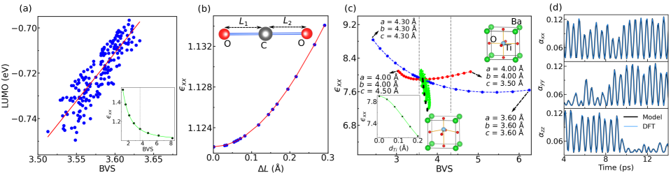
Figure 1: (Color online) (a) LUMO (eV) vs BVS (blue circles) and the linear fit (red line) for CO₂ structures generated by MD at 300 K. Inset: the Lorentzian function fit (green) of $\epsilon_{xx}$ to BVS (black dots) for symmetrically stretched CO₂. Gray dotted line (Inset): BVS (3.64) of CO₂ at DFT-relaxed position. (b) $\epsilon_{xx}$ vs $\Delta L$ ($\mid L_{1}$ - $L_{2}\mid$) for CO₂ for BVS = 3.64 (blue circles) with the Lorentzian fit (red). $L_{1}$ and $L_{2}$ are C-O bond lengths (see inset). (c) $\epsilon_{xx}$ vs Ti BVS for five-atom BTO for isotropic volume change of cubic centrosymmetric BTO (blue), compression and extension of the $z$-axis of centrosymmetric BTO (red), Ba and Ti shifted along $x$-direction while O are fixed at centrosymmetric positions for cubic BTO with $a$ = 4.00 Å (black circles), Ba and Ti fixed at the centrosymmetric positions while O are shifted along $x$-direction for cubic BTO with $a$ = 4.00 Å (green circles). Gray dotted lines: Minimum (3.56) and maximum (4.33) Ti BVS from 5-atom MD in the temperature range 200-1000 K. Bottom corner inset: Lorentzian fit (green) of $\epsilon_{xx}$ vs off-centre displacement of Ti ($d_{Ti}$ (Å)) (black dots), where Ba and O are at centrosymmetric position. (d) Polarizability ($\alpha_{xx}$, $\alpha_{yy}$ and $\alpha_{zz}$) trajectory using model and DFT for CO₂ at 300 K.

Alternatively, the polarizability surface (i.e. polarizability as a function of atomic coordinates) can be modeled using either polynomial expansion or deep learning methods to enable direct calculation of Raman spectra from MD trajectories Omodemi et al. (2022); Sommers et al. (2020); Luo et al. (2022). However, both of these approaches require a large database of training structure for the parameterization of the model. Deep learning models are also more computationally expensive (by a factor of up to 100) than atomistic potentials  Mo et al. (2022); Wu et al. (2021); Zhang et al. (2018); Jia et al. (2020). However, atomistic models for polarizability similar in spirit to the atomistic models for evaluation of energy and forces from atomic coordinates have not been reported to date for complex systems with multi-center bonding. This is may be due to the assumption that the response of electronic structure to the incident electromagnetic field and its dependence on atomic coordinates in a solid-state material are too complicated to be decomposed into contributions of individual atoms and expressed by a simple atomistic model and thus can only be modeled using quantum mechanical approaches.

Here, we demonstrate that by considering the effect of the dynamical changes in the structure and chemical bonding in molecules or materials together with the second-order perturbation theory expression for electronic polarizability, a computationally efficient and atomistically-interpretable model with few adjustable parameters characterizing the evolution of electronic polarizability in terms of atomic coordinates can be derived. We then apply the model with $\leq$ 10 parameters for the calculation of Raman spectra from MD simulations using CO₂, water clusters ((H₂O)_n: $n$ = 1-6, 8), and BaTiO₃ (BTO) and CsPbBr₃ (CPB) systems with supercells of up to $\approx$ 500,000 atoms to demonstrate the accuracy of this approach.

From perturbation theory, the polarizability tensor ($\alpha$) can be represented as Luber et al. (2014); Long (2002)

$$\alpha_{ij}\propto\sum_{\gamma\neq 0}\frac{\langle\Phi_{0}\mid\hat{p_{i}}\mid\Phi_{\gamma}\rangle\langle\Phi_{\gamma}\mid\hat{p_{j}}\mid\Phi_{0}\rangle}{\hbar(\omega_{\gamma}-\omega_{0})}$$

where $\mid\Phi_{0}\rangle$ and $\mid\Phi_{\gamma}\rangle$ are ground and excited states, $\hat{p_{i}}$ is the induced electric dipole operator due to external field, and $\hbar$($\omega_{\gamma}-\omega_{0}$) is the energy difference between excited and ground states. Thus, the atomistic model must take into account the effect of the changes of the bonding and the coupling between the individual bonds on this perturbation theory expression. The denominator ($\omega_{\gamma}-\omega_{0}$) can be related to the second moment of the local density of states and thus the bond valence sum (BVS)  Sutton (1993); Liu et al. (2013) defined as

$$\textnormal{BVS}=\sum_{i}exp((d^{0}_{AB}-d_{i})/b)$$ (1)

where $d^{0}_{AB}$ and $d_{i}$ are the bond valence parameter and bond length for the bond between atoms $A$ and $B$, respectively, $b$ (= 0.37 Å) is an universal constant Brese and O’Keeffe (1991). Therefore, BVS rather than the individual bond lengths characterizes the changes in the local bonding environment and should be related to the $\alpha$. We use the CO₂ molecule as a simple model system to demonstrate the relationship between BVS and the LUMO energy (see Fig. 1 (a)). Plotting $\boldsymbol{\epsilon}$ versus BVS for a symmetric stretching of CO₂, we find that the atom’s polarizabilty ($\boldsymbol{\alpha}$) due to symmetrically stretched bond can be characterized by Lorentzian function of the BVS of that atom (see inset of Fig. 1 (a)).

Since BVS is insensitive to the details of the local atomic arrangement, the effect of local asymmetry on $\boldsymbol{\alpha}$ must be taken into account separately. We investigate the influence of the asymmetry on $\boldsymbol{\alpha}$ by plotting $\epsilon_{xx}$ versus the bond length difference ($\Delta L$) in CO₂ for a fixed BVS (3.64) so that the values of ($\omega_{\gamma}$ - $\omega_{0}$) show only small variation (Fig. 1 (b)). It is observed that $\boldsymbol{\alpha}$ shows a Lorentzian dependence on the asymmetry of CO₂.

To understand the relationship between $\boldsymbol{\alpha}$ and atomic coordinates, BVS and asymmetry in a more complicated solid-state system, we considered the following cases for a 5-atom BTO cell: (a) isotropic volume change of cubic centrosymmetric BTO, (b) Ba and Ti displacing along $x$ direction and O fixed at centrosymmetric position for cubic BTO where lattice constant = 4.00 Å and (c) Ba and Ti fixed at the centrosymmetric positions and O displacing along $x$ direction for cubic BTO where lattice constant = 4.00 Å, (d) Anisotropic volume change (tetragonal distortion) of centrosymmetric BTO. The plots of $\boldsymbol{\alpha}$ versus Ti BVS for cases (a)-(d) are shown in Fig. 1 (c). For (a), we observed a Lorentzian dependence of $\boldsymbol{\alpha}$ on BVS in the physically relevant range of $\approx$ 3.5-4.5. For (b) and (c), despite the small variation in BVS, a strong change in $\boldsymbol{\alpha}$ is observed with $\boldsymbol{\alpha}$ decreasing strongly with greater off-center atomic displacement (asymmetry). The dependence of $\boldsymbol{\alpha}$ on asymmetry (off-center displacement of Ti) also follows a Lorentzian dependence (see inset of Fig. 1 (c)). For (d), we observe an interesting trend of $\boldsymbol{\alpha}$ first decreasing and then increasing with the change in the BTO aspect ratio. The results for cases (a)-(c) show that similar to the CO₂ molecule, $\boldsymbol{\alpha}$ for the solid-state BTO shows Lorentzian dependence on the BVS and the asymmetric atomic displacement. The results for (d) can be explained by considering that more isolated atoms have higher $\boldsymbol{\alpha}$ than the corresponding more bonded system (in part due to lower ($\omega_{\gamma}-\omega_{0}$)) and that BTO with either very low or very high aspect ratio will contain O atoms (axial O atoms for high aspect ratio, equatorial O atoms for low aspect ratio) that participate only weakly in bonds with Ti. For high aspect ratio, the long distances between Ti and axial O atoms will make the O atoms more non-bonding and will increase $\boldsymbol{\alpha}$. For low aspect ratio, the very short distances between Ti and axial O atoms will lead to the concentration of the bonding along the $z$-axis, leaving the O atoms in the $xy$ plane with weak bonds to Ti even for the Ti-O distances of 2.0 Å. To represent this effect, we introduce dynamical charge $m$ for evaluation of the actual bond order of a given Ti-O bond taking into account the competition for bonding charge with all other bond.

Based on the insights obtained from the relationships described above, we define the bond polarizability $\alpha_{ij}$ between atoms $A$ and $B$ where sum over bond polarizability gives total $\boldsymbol{\alpha}$, as

$$\begin{split}\alpha_{ij}=[A_{\parallel}^{s}*A_{\parallel}^{a}+B_{\parallel}^{s}*B_{\parallel}^{a}]*(\frac{R_{i}R_{j}}{R^{2}})\\ +[A_{\perp}^{s}*A_{\perp}^{a}+B_{\perp}^{s}*B_{\perp}^{a}]*(\delta_{ij}-\frac{R_{i}R_{j}}{R^{2}})\end{split}$$ (2)

where dielectric constant ($\epsilon_{ij}$) is related to $\alpha_{ij}$ as, $\alpha_{ij}$ $\propto$ ($\epsilon_{ij}$ - $\delta_{ij}$). Here $i$, $j$ denote $x$, $y$ or $z$ axes. The first and second expression of $\alpha_{ij}$ give the parallel and perpendicular contribution of the bond to $\alpha_{ij}$, respectively. $A_{\parallel}^{s}$ ($B_{\parallel}^{s}$) and $A_{\parallel}^{a}$ ($B_{\parallel}^{a}$) describe the effects of the symmetric and asymmetric bond length changes on the contribution of $A$ ($B$) ion to the polarizability along the $A-B$ bond direction. Similarly, $A_{\perp}^{s}$ ($B_{\perp}^{s}$) and $A_{\perp}^{a}$ ($B_{\perp}^{a}$) describe the effects of the symmetric and asymmetric bond length changes on the contribution of $A$ ($B$) ion to the polarizability perpendicular to the $A-B$ bond direction. Here R defines the $A-B$ bond length. $\delta_{ij}$ = 1 if $i$ = $j$ and $\delta_{ij}$ = 0 if $i$ $\neq$ $j$, following the approach developed for the bond polarizability model Hermet et al. (2006).

We define $A_{\parallel}^{s}$, $A_{\parallel}^{a}$, $B_{\parallel}^{s}$, $B_{\parallel}^{a}$, $A_{\perp}^{s}$, $A_{\perp}^{a}$, $B_{\perp}^{s}$ and $B_{\perp}^{a}$ using a simple Lorentzian function. Thus we have the following expressions,
$A_{\parallel}^{s}=\frac{a_{1}^{2}}{(x_{A}^{s}-a_{2})^{2}+a_{3}^{2}}$, $B_{\parallel}^{s}=\frac{a_{1}^{2}}{(x_{B}^{s}-a_{2})^{2}+a_{3}^{2}}$, $A_{\perp}^{a}$ = $\frac{a_{8}^{2}}{(y_{A,\perp}^{a})^{2}+a_{8}^{2}}$
$A_{\perp}^{s}=\frac{a_{4}^{2}}{(x_{A}^{s}-a_{5})^{2}+a_{6}^{2}}$, $B_{\perp}^{s}=\frac{a_{4}^{2}}{(x_{B}^{s}-a_{5})^{2}+a_{6}^{2}}$, $B_{\perp}^{a}$ = $\frac{a_{10}^{2}}{(y_{B,\perp}^{a})^{2}+a_{10}^{2}}$
$A_{\parallel}^{a}$ = $\frac{a_{7}^{2}}{(y_{A,\parallel}^{a})^{2}+a_{7}^{2}}$, $B_{\parallel}^{a}$ = $\frac{a_{9}^{2}}{(y_{B,\parallel}^{a})^{2}+a_{9}^{2}}$

In the above expressions $a_{1}$, $a_{2}$, $a_{3}$, $a_{4}$, $a_{5}$, $a_{6}$, $a_{7}$, $a_{8}$, $a_{9}$, and $a_{10}$, are the constants in the Lorentzian expressions to be fit to DFPT-calculated polarizability data. $x_{A}^{s}$, $x_{B}^{s}$, $y_{A}^{a}$ and $y_{B}^{a}$ are determined from the atomic coordinates. $x_{A}^{s}$ is defined as, $x_{A}^{s}=BVS\times\frac{m}{m_{0}}$ here $BVS$ = total bond valence of $A$ given by Eq. 1, $m$ is the dynamical formal charge of $A$ ion that varies depending on the environment, and $m_{0}$ is the formal charge of $A$ (e.g. 4 for C and Ti in CO₂ and BTO and 2 for O). The dynamical charge state is defined as, $m$ = $\sum_{k}[\frac{BV_{k}}{BVS_{k}}\times m_{0k}]$. Here, $k$ is the neighbor bond index of $A$. $BV_{k}$ is the bond valence of the $k$-th $A$-$B$ bond. $BVS_{k}$ and $m_{0k}$ are the total bond valence and formal charge of $B$ ion residing at $k$-th $A$-$B$ bond, respectively. $x_{s,B}$ is defined in similar manner to $x_{s,A}$.

Then, $y_{A}^{a}$ is the asymmetric displacement of $A$ ion from the center of mass of the nearest-neighbor $B$ ions. $y_{A,\parallel}^{a}$ and $y_{A,\perp}^{a}$ are the parallel and perpendicular projection of the asymmetric displacement on the $A$-$B$ bond. $y_{B}^{a}$ is the asymmetric displacement of $B$ ion from the center of mass of the nearest-neighbor $A$ ions. $y_{B,\parallel}^{a}$ and $y_{B,\perp}^{a}$ are defined similarly to $y_{A,\parallel}^{a}$ and $y_{A,\perp}^{a}$.

To calculate these unknown parameters of Lorentzian expressions, we first calculated polarizability trajectory ($\alpha_{DFT}$) from density functional theory (DFT) for a small number of points along the MD trajectory. We then optimized the parameters in the our model for $\alpha_{ij}$ (Eq. 2) to reproduce the $\alpha_{DFT}$ using simulated annealing algorithm, with the optimized parameters given in SM. A comparison between the DFT $\alpha$ trajectories and the model $\alpha$ trajectories for CO₂ are presented in Fig. 1 (d), showing excellent agreement.

Figure 2: (Color online) (a) Polarizability ($\alpha_{xx}$) trajectory from model and DFT for H₂O molecule at 300 K. (b) Raman spectra of H₂O clusters ((H₂O)_n: $n$ = 1-6, 8). First, second and third panels show spectra of H₂O, (H₂O)₂ and (H₂O)₃ from model and DFT respectively. Fourth panel: model spectra for (H₂O)₄ (green) and (H₂O)₅ (red). Fifth panel: model spectra for (H₂O)₆ (green) and (H₂O)₈ (red).

Next, we apply our model to calculate Raman spectra of water clusters ((H₂O)_n: $n$ = 1-6, 8). Fig. 2 (a) show the comparison of polarizability ($\alpha_{xx}$) trajectory at 300 K as calculated from DFT and the model for H₂O. Clearly, the model trajectory captured the main features of the DFT trajectory. We then calculate the Raman spectra of H₂O from the atomic coordinates obtained from MD simulations, with the results shown in Fig. 2 (b)(First panel). The spectrum calculated from the DFT-obtained polarizability time autocorrelation function as shown in the same plot gives a good agreement between them. The spectra consist of three peaks, corresponding to the H-O-H bending mode (the small peak around 1600 cm^-1), and the symmetric and asymmetric O-H stretching modes at around 3800 cm^-1 and 3900 cm^-1 respectively. These results are in agreement with available experimental Raman spectra  Brooker et al. (1989).

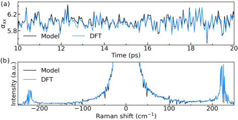
Figure 3: (Color online) (a) Polarizability ($\alpha_{xx}$) trajectory, (b) Raman spectra from model and DFT for BaTiO₃ (5 atoms cell) at 300 K.

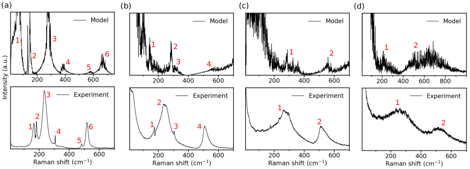
Figure 4: (Color online) Raman spectra of single crystal BTO for different phases (a) rhombohedral, (b) orthorhombic, (c) tetragonal, and (d) cubic from model and experiment. The temperatures for (a), (b), (c) and (d) are 40, 92, 110 and 160 K respectively (top panel), and 123, 233, 333 and 423 K respectively (bottom panel).

To examine whether our model can be used to capture the effects of hydrogen bonding on Raman spectra, we compared the DFT and model Raman spectra of (H₂O)₂ and (H₂O)₃ clusters as calculated using the same constants as those used for single H₂O (see Fig. 2(b)), which also show a good agreement between model and DFT results. This shows that the model can handle systems with hydrogen-bonded water because the effect of hydrogen bonding on polarizability is mostly due to the changes of the H₂O geometry induced by hydrogen bonds, whereas hydrogen bonds induce only small changes in the response of the electron cloud to electric field for a given H₂O geometry. Due to the computational constraints, the above-discussed DFT-derived spectra were obtained for runs of 44 ps with a time step of 0.003 ps and the same simulation duration and time step and trajectories were also used for the calculation of model-derived spectra. In the SM, we present the more accurate model Raman spectra of H₂O, (H₂O)₂ and (H₂O)₃ derived from atomistic (Babin et al. (2014); Eastman et al. (2017); Samala and Agmon (2019)) simulation trajectories for 3 ns with a time step of 0.001 ps. We have also calculated the Raman spectra for (H₂O)₄, (H₂O)₅, (H₂O)₆ and (H₂O)₈ using the longer atomistic potential trajectories as shown in the fourth and fifth panels of Fig. 2(b), respectively. The peak positions of the ((H₂O)_n, $n$ = 1-6, 8) are in good agreement with the results in the literature Samala and Agmon (2019).

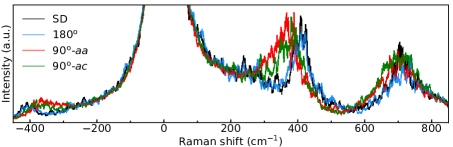
Figure 5: (Color online) Raman spectra for different Domain structure of BTO.

Next we apply the model to the classic ferroelectric BTO for which an atomistic potential is available Qi et al. (2016), enabling large MD simulations. We use the $ab$ $initio$ MD $\boldsymbol{\alpha}$ data as calculated using 10-atom BTO cell to fit the parameters in Eq. 2 for the TiO₆ octahedron only. We ignore the contribution of the BaO₁₂ polyhedra to $\boldsymbol{\alpha}$ because it is small relative to that of TiO₆ due to predominantly Ti 3$d$ character of the conduction band (see the SM for more information). In Fig. 3 (a), we present the trajectories of $\alpha_{xx}$ at 300 K as calculated using DFT and the parameterized model, respectively. It is observed here as well that the model $\alpha_{xx}$ trajectory is in good agreement with the DFT trajectory. For direct comparison of the model with DFT results, we calculated Raman spectra using DFT $\alpha_{xx}$ and model $\alpha_{xx}$ with the results shown in Fig. 3 (b) . The figure shows that the DFT-based and model-based spectra are in good agreement.

Next, we considered a large simulation cell of single-domain BTO with the dimensions of 16$\times$16$\times$16 (20,480 atoms) in order to examine the accuracy of the model in characterizing the phase transition of BTO. We calculated the trajectories using atomistic MD with the bond-valence potential for different temperature between 10 K and 160 K which capture all of the phases of BTO for this potential . The evolution of polarization with time for all of these phases is presented in the SM. We then used the same constants as obtained for 10-atom BTO cell to calculate the Raman spectra of the single-domain 16$\times$16$\times$16 BTO for all the considered temperatures. Fig. 4 compares the results obtained by our model calculations with the experimentally obtained spectra of single-crystal BTO (see SM also). Examination of the theoretical Raman spectra shows that rhombohedral, orthorhombic, tetragonal and cubic phases are achieved at $<$80 K, 90-95 K, 100-130 K and $>$160 K, respectively. This corresponds to the experimentally observed phase transitions at 183, 278 and 393 K due to the underestimation of the phase transition temperatures by DFT-based potentials Qi et al. (2016). Additionally, with the increase of temperature, both experimental and theoretical spectra show peak broadening. For the rhombohedral phase at 40 K in the theoretical results, the peaks below 200 cm^-1 match well the R-phase experimental peaks below 200 cm^-1. The two peaks in the range of 200-500 cm^-1 in the theoretical spectra correspond to the two peaks in the 200-400 cm^-1 in the experimental spectra. The peaks between 500 and 700 cm^-1 in theoretical spectra correspond to the peak around 500 cm^-1 observed experimentally. The peak in the high wavenumber region as observed theoretically (see SM) is also consistent with the experimental peak above 700 cm^-1 Deluca et al. (2018). Similarly, the comparison between theoretical results and experimental results shows good agreement for other phases of BTO. We also applied the model to CPB halide perovskite and obtained good agreement between DFT and model polarizability trajectories and Raman spectra (see SM).

To further demonstrate the utility of the model, we applied it to the Raman spectra of different ferroelectric domain structures of BTO to show that Raman spectra can distinguish between the different domain phases and these difference can be interpreted using the atomistic polarizability model. We considered single-domain, 180^∘ domain, 90^∘($aa$) domain and 90^∘($ac$) domain structures of BTO based on MD simulations using 120$\times$120$\times$6 supercell (432,000 atoms) with the obtained Raman spectra shown in Fig. 5. It is clear that different domain variants can be detected based on the differences between their respective Raman spectra. These simulations also show that Raman spectra can be obtained for large supercells at essentially negligible computational cost that is only $\sim$ 50% of the computational cost of BV potential MD simulations. (70 CPU hours required for MD simulations and 35 CPU hours required for each Raman spectrum calculations on 32 core machine).

To summarize, we have demonstrated that a simple, physically-based atomistic model with only 10 adjustable parameters can accurately represent the changes in the electronic polarizability of complex system such as BTO. Due its physical basis, the model is much more compact than the polynomial expansion (128 adjustable parameters for H₂O molecule Omodemi et al. (2022)) and the deep-learning models of the polarizability tensor. This enables efficient calculations of Raman spectra from large-scale MD simulations with only modest computational resources as well as atomistic and local analysis of the contributions to Raman spectra for the interpretation of Raman spectroscopy results.

References

- Butler et al. (2016) H. J. Butler, L. Ashton, B. Bird, G. Cinque, K. Curtis, J. Dorney, K. Esmonde-White, N. J. Fullwood, B. Gardner, P. L. Martin-Hirsch, M. J. Walsh, M. R. McAinsh, N. Stone, and F. L. Martin, Nature Protocols 11, 664 (2016).
- Zhang et al. (2015) X. Zhang, X.-F. Qiao, W. Shi, J.-B. Wu, D.-S. Jiang, and P.-H. Tan, Chem. Soc. Rev. 44, 2757 (2015).
- Yaffe et al. (2017) O. Yaffe, Y. Guo, L. Z. Tan, D. A. Egger, T. Hull, C. C. Stoumpos, F. Zheng, T. F. Heinz, L. Kronik, M. G. Kanatzidis, J. S. Owen, A. M. Rappe, M. A. Pimenta, and L. E. Brus, Phys. Rev. Lett. 118, 136001 (2017).
- Thomas et al. (2013) M. Thomas, M. Brehm, R. Fligg, P. Vöhringer, and B. Kirchner, Phys. Chem. Chem. Phys. 15, 6608 (2013).
- Baroni et al. (2001) S. Baroni, S. de Gironcoli, A. Dal Corso, and P. Giannozzi, Rev. Mod. Phys. 73, 515 (2001).
- Guha et al. (1996) S. Guha, J. Menéndez, J. B. Page, and G. B. Adams, Phys. Rev. B 53, 13106 (1996).
- Wirtz et al. (2005) L. Wirtz, M. Lazzeri, F. Mauri, and A. Rubio, Phys. Rev. B 71, 241402 (2005).
- Hermet et al. (2006) P. Hermet, N. Izard, A. Rahmani, and P. Ghosez, The Journal of Physical Chemistry B 110, 24869 (2006).
- Hashemi et al. (2019) A. Hashemi, A. V. Krasheninnikov, M. Puska, and H.-P. Komsa, Phys. Rev. Mater. 3, 023806 (2019).
- Kou et al. (2020) Z. Kou, A. Hashemi, M. J. Puska, A. V. Krasheninnikov, and H.-P. Komsa, npj Computational Materials 6, 59 (2020).
- Parker et al. (1967) J. H. Parker, D. W. Feldman, and M. Ashkin, Phys. Rev. 155, 712 (1967).
- Nilsen and Skinner (1968) W. G. Nilsen and J. G. Skinner, The Journal of Chemical Physics 48, 2240 (1968).
- Livneh and Spanier (2015) T. Livneh and J. E. Spanier, 2D Materials 2, 035003 (2015).
- Omodemi et al. (2022) O. Omodemi, S. Sprouse, D. Herbert, M. Kaledin, and A. L. Kaledin, Journal of Chemical Theory and Computation 18, 37 (2022).
- Sommers et al. (2020) G. M. Sommers, M. F. Calegari Andrade, L. Zhang, H. Wang, and R. Car, Phys. Chem. Chem. Phys. 22, 10592 (2020).
- Luo et al. (2022) R. Luo, J. Popp, and T. Bocklitz, Analytica 3, 287 (2022).
- Mo et al. (2022) P. Mo, C. Li, D. Zhao, Y. Zhang, M. Shi, J. Li, and J. Liu, npj Computational Materials 8, 107 (2022).
- Wu et al. (2021) J. Wu, Y. Zhang, L. Zhang, and S. Liu, Phys. Rev. B 103, 024108 (2021).
- Zhang et al. (2018) L. Zhang, J. Han, H. Wang, R. Car, and W. E, Phys. Rev. Lett. 120, 143001 (2018).
- Jia et al. (2020) W. Jia, H. Wang, M. Chen, D. Lu, L. Lin, R. Car, E. Weinan, and L. Zhang, in SC20: International Conference for High Performance Computing, Networking, Storage and Analysis (2020) pp. 1–14.
- Luber et al. (2014) S. Luber, M. Iannuzzi, and J. Hutter, The Journal of Chemical Physics 141, 094503 (2014).
- Long (2002) D. A. Long, The Raman Effect (John Wiley & Sons, Ltd, 2002).
- Sutton (1993) A. P. Sutton, Electronic structure of materials, Oxford science publications (Clarendon Press, Oxford, 2004 - 1993).
- Liu et al. (2013) S. Liu, I. Grinberg, H. Takenaka, and A. M. Rappe, Phys. Rev. B 88, 104102 (2013).
- Brese and O’Keeffe (1991) N. E. Brese and M. O’Keeffe, Acta Crystallographica Section B 47, 192 (1991).
- Note (1) = normalization factor( - 1) and the normalization factor is related to the amount of vacuum in the unit cell used to calculate . Both of these give similar expressions. Therefore, while plotting we have shown DFT-calculated . However, in text we always use .
- Brooker et al. (1989) M. H. Brooker, G. Hancock, B. C. Rice, and J. Shapter, Journal of Raman Spectroscopy 20, 683 (1989).
- Babin et al. (2014) V. Babin, G. R. Medders, and F. Paesani, Journal of Chemical Theory and Computation 10, 1599 (2014).
- Eastman et al. (2017) P. Eastman, J. Swails, J. D. Chodera, R. T. McGibbon, Y. Zhao, K. A. Beauchamp, L.-P. Wang, A. C. Simmonett, M. P. Harrigan, C. D. Stern, R. P. Wiewiora, B. R. Brooks, and V. S. Pande, bioRxiv (2017), 10.1101/091801.
- Samala and Agmon (2019) N. R. Samala and N. Agmon, The Journal of Physical Chemistry B 123, 9428 (2019).
- Qi et al. (2016) Y. Qi, S. Liu, I. Grinberg, and A. M. Rappe, Phys. Rev. B 94, 134308 (2016).
- Note (2) Though this is not the actual spectra as we considered trajectory for small time with large time step, these results indicate the accuracy of this model.
- Note (3) Since the BV potential is based on DFT calculations, it underestimates the Curie temperature of BTO due to the underestimation of the O6 rotation energy cost by DFT as shown in previous work Qi et al. (2016).
- Deluca et al. (2018) M. Deluca, Z. G. Al-Jlaihawi, K. Reichmann, A. M. T. Bell, and A. Feteira, J. Mater. Chem. A 6, 5443 (2018).