On the interplay between activity, elasticity and liquid transport
in self-contractile biopolymer gels

Abstract

Active gels play an important role in biology and in inspiring biomimetic active materials, due to their ability to change shape, size and create their own morphology; the relevant mechanics behind these changes is driven by self-contraction and liquid flow. Here, we couple contraction and liquid flow within a nonlinear mechanical model of an active gel disc to discuss how contraction dynamics inherits length scales which are typical of the liquid flow processes. The cylindrically symmetric model we present, which recapitulate our previous theoretical modeling in its basic lines, reveals that when also liquid flow is taken into account, the aspect ratio of the disc is not the only geometrical parameter which characterizes the contraction dynamics of the gel. The analyses we present provide important insights into the dependence of contraction dynamics on geometry and allow to make some progress in designing materials which can be adapted for different applications in soft robotics.

I Introduction

Self-contractile active gels are usually generated by polymerizing actin in the presence of cross-linkers and clusters of myosin as molecular motors[1, 2, 3, 4, 5]. Mechanics of active gels present interesting characteristics: self-contractions generate internal stresses and stiffen the material, so driving the network into a highly nonlinear, stiffened regime [2]; morphing from flat to curved geometries can be expected when thin discs of active gels are considered [5]; boundaries affect morphing [3].
The first models [6, 7, 8] of these materials were based on a physical description of the contraction dynamics within the framework of active generalized hydrodynamics: transient force dipoles are generated by myosin pulling on actin chains and creating active contractile stresses. These models are very accurate in modeling the contraction dynamics, looking at the network mesh scale, and less interested in coupling that dynamics with the nonlinear mechanics of active gels, which is also strongly affected by liquid flow [5].
Recently, the mechanics of active gels have been at the centre of a few theoretical studies, set within the framework of nonlinear mechanics, where the interactions between elastic stresses and liquid flow have been investigated [9, 10, 11, 12, 13]. In [10], a dynamic cross-linking mechanism is introduced to take into account the active behaviour of the gel. It drives an evolution of the mechanical stiffness of the polymeric network and an increase of the strain energy. The approach exploited in [9, 11, 12, 13] by some of the authors is quite different: the activity in the gel is modeled as an external remodeling force that drives the microscopic reorganization of the network due to activity and competes with the passive deformation of the gel due to elasticity and liquid flow . Network remodeling drives both the evolution of the mechanical stiffness of the polymer and the chain shortening, which are two of the main mechanisms [5, 7] evidenced in the experiments [5].
In the present work, we start from that approach [13] to focus on the interactions between activity, elasticity and liquid diffusion in active gels, which are largely unexplored. The variety of of phenomena to be understood is wide, and robust macroscopic models of contractile networks can inspire further experiments to improve the control of the active characteristics of the gel and of its relevant mechanics.
The point we discuss here is about the competitive roles of contraction and liquid flow in driving the mechanics of the active gel. We refer to a specific problem, whose analysis has been inspired by the work presented in Ref.5, where the contraction dynamics of an active gel disc, whose geometry is defined by radius and thickness, has been followed and described with great details. Through the analysis of the problem, we’ll show how: (i) gel dynamics inherits length scales which are typical of the liquid flow processes; (ii) two different regimes characterize the dynamics of the disc, which can be ascribed to gel contraction and to liquid flow; (iii) the gel dimensions’ aspect ratio (radius to thickness) impact on the gel dynamics and affects also stress distribution.
The model is presented in Sec. II and III. Sec. IV describes the equilibrium states of the active gel and Sec. IV deals with contraction dynamics.

II Active volume and polymer fraction

Differently from passive polymer gels, active gels have the ability to remodel their mesh by self-contractions. The key elements of our model of active gel are here contrasted with the standard Flory-Rehner model of passive gels, which is at the bases of the stress-diffusion theories describing the chemo-mechanical interactions in swollen gels [15, 16, 17, 18, 19, 12].
A key variable in the Flory-Rehner model is the polymer fraction $\phi$, defined as the ratio between the volume of the polymer $V_{p}$ and the total volume $V$:

$$\phi=\frac{V_{p}}{V},\quad\textrm{with}\quad V=V_{p}+V_{s},$$ (II.1)

where $V_{s}$ is the volume of solvent content. This formula is based on the assumption that a given mass of polymer occupies a constant volume $V_{p}$, be it dry or not; thus, any volume increase must be entirely due to the solvent volume $V_{s}$. Moreover, the Flory-Rehner model assumes that the polymer chains are not stretched at dry state, and that it is the solvent absorption that stretches these chains. Equilibrium is given by a balance between the elastic energy, which prefers unstretched chains, and the mixing energy that favours swelling and thus requires stretching to accommodate more solvent.

The active gel model removes the assumption of constant polymer volume, and considers the volume that can be occupied by a given mass of dry polymer as an additional state variable, named active volume $V_{a}$. The volume $V_{a}$ can vary because of a change of the mean free-length of the polymer chains, that is, of the average mesh size $\xi_{a}$ measured at dry conditions; thus, $V_{a}$ can be considered as a coarse-grained modeling of the microscopic arrangement of the polymer chains. It turns out that a change of $V_{a}$ also describes a change of the effective stiffness of the gel. For the active gel model, the polymer fraction is measured by

$$\phi=\frac{V_{a}}{V},\quad\textrm{with}\quad V=V_{a}+V_{s}.$$ (II.2)

The hypothesis that the polymer chains are not stretched at dry state is maintained; thus, the thermodynamical equilibrium is still a consequence of the balance between elastic energy and mixing energy. The new formula $\phi=V_{a}/(V_{a}+V_{s})$ describes interactions between activity and solvent content. For example, we might have the same polymer fraction $\phi$ with different pairs $V_{a}$, $V_{s}$:

$$\phi=\frac{V_{ao}}{V_{ao}+V_{so}}=\frac{V_{a1}}{V_{a1}+V_{s1}}\quad\Rightarrow\quad\frac{V_{a1}}{V_{ao}}=\frac{V_{s1}}{V_{so}}\,,$$ (II.3)

as $1/\phi=1+V_{so}/V_{ao}=1+V_{s1}/V_{a1}$. From (II.3), it follows that a contraction of the polymer network yields a proportional reduction of its solvent content. For very soft gels, as is our case, $\phi$ can be very small and a small volume contraction of $V_{a}$ can yield a huge expulsion of solvent volume $V_{s}$. As example, by assuming $V_{ao}=1$ mm³ and $V_{so}=1000$ mm³, we have $\phi=1/1001$; a contraction that halves the polymer volume yields $V_{a1}=0.5$ mm³ and $V_{s1}=500$ mm³. Following our example, the average mesh size $\xi_{a}$ corresponding to the two active volumes $V_{ao}$ and $V_{a1}=V_{ao}/2$ scales as $\xi_{a1}/\xi_{ao}=(1/2)^{1/3}\simeq 0.8$. It is worth remembering that $\xi_{a}$ is the mesh size of the unstretched chains, which determines the so-called spontaneous metric of the network, whereas the actual mesh size $\xi$ is related to the actual swollen volume and determines the current metric of the network: $\xi\propto(V_{a}+V_{s})^{1/3}$. Both $\xi_{a}$ and $\xi$ may be very different from the reference mesh size $\xi_{d}$ of the dry polymer, due to activity and liquid flow, see figure 2.
In the mathematical model, the microscopic arrangement of the polymer chains (from now on, the remodeling) is driven by a new evolution equation with its own source term, which is represented by the external remodeling force that maintains the system steady, or that drives it out of equilibrium [20]. It affects the solvent flow in the gel: a contraction of the polymer mesh yields a liquid flow towards the boundary of the body, favouring its release. Indeed, as we shall shortly review in the following, the polymer fraction $\phi$ depends on $V_{a}$ through a balance equation of solvent concentration, driven by a Flory-Rehner thermodynamics, which is so affected by gel activity.

III Stresses, liquid fluxes and self-contractions

The active gel model is formulated in the framework of 3D continuum physics, see [9, 11] for details, which allow to set up initial-boundary value problems well suited to describe real experiments. Inspired by the experiments in [5], we consider a disc-like continuum body: at the initial time, it is a fully swollen, flat gel disc $\mathcal{B}_{o}$, having radius $R_{o}$ and thickness $H_{o}$, which is $\lambda_{o}$ times larger then the corresponding dry disc $\mathcal{B}_{d}$ (see figure 1, panel a).

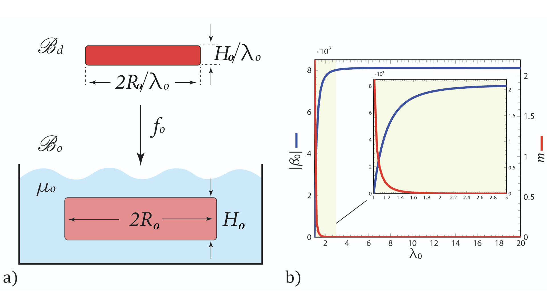
Figure 1: (a) Dry configuration $\mathcal{B}_{d}$ and swollen initial one $\mathcal{B}_{o}$: $H_{o}$ and $2R_{o}$ are thickness and diameter of $\mathcal{B}_{o}$ when the bath has chemical potential $\mu_{o}$. (b) Free-swelling stretch $\lambda_{o}$ versus the energy ratio $m=G\Omega/RT$ at $\mu_{o}=0$ (red) and versus the bulk source $\beta_{o}$ (blue) needed to maintain $\lambda_{o}$ in thermodynamical equilibrium; the lower the ratio $m$ (that is, mixing energy larger than the elastic one), the higher the bulk source $\beta_{o}$.

The region $\mathcal{B}_{d}$ is assumed as the reference configuration of the active gel disc and the mathematical model describes the state of the gel by using three state variables: the solvent concentration per unit of dry volume $c_{d}:\mathcal{B}_{d}\times\mathcal{T}\to\mathcal{R}$ ($[c_{d}]=$mol/m³); the mechanical displacement $\mathbf{u}:\mathcal{B}_{d}\times\mathcal{T}\to\mathcal{V}$ ($[\mathbf{u}]=$m); the active contractions $\mathbf{F}_{a}:\mathcal{B}_{d}\times\mathcal{T}\to\mathbb{L}\mathtt{in}$ ($[\mathbf{F}_{a}]=$1), usually called remodeling tensor. Here, $\mathcal{R}$, $\mathcal{V}$, and $\mathbb{L}\mathtt{in}$ denote a scalar, a vector and a tensor, respectively; $\mathcal{T}$ is the time interval under study (see [11, 12] for details).

Solvent concentration $c_{d}$ and displacement $\mathbf{u}$ are the standard state variables based on Flory-Rehner model; the active contraction $\mathbf{F}_{a}$ is the new variable used to describe active gels. The tensor $\mathbf{F}_{a}$ is the 3D equivalent of the volume $V_{a}$ mentioned in the previous section: it describes not only the change in volume, but also the macroscopic changes in length and angles of the polymeric network due to self-contractions (see figure 2). The time-dependent symmetric tensor field $\mathbf{C}_{a}=\mathbf{F}_{a}^{T}\mathbf{F}_{a}$ accounts for the reduction of the free length of the polymer chains, due to self-contraction, and describes the spontaneous metric of the gel.

Given the deformation gradient $\mathbf{F}=\mathbf{I}+\nabla\mathbf{u}$, the key relations (II.2) are now represented in terms of Jacobian determinants

$$\phi=\frac{J_{a}}{J},\quad\textrm{with}\quad J=\textrm{det}\,\mathbf{F}=J_{a}+\Omega\,c_{d},\quad J_{a}=\textrm{det}\,\mathbf{F}_{a}\,;$$ (III.4)

it holds $\xi_{a}/\xi_{d}\simeq J_{a}^{1/3}$ and $\xi/\xi_{d}\simeq J^{1/3}$. Equations (III.4) imply that any actual volume change $J$ is the sum of a volume change of the active mesh $J_{a}$, plus the volume of the solvent $\Omega\,c_{d}$. Polymer fraction $\phi$ delivers a measure of the gel density, which increases when solvent content decreases and depends on the volume change of the active mesh, as equations (III.4) indicate.
The deformation of the actual mesh with respect to the unstretched one is measured by $\mathbf{F}_{e}=\mathbf{F}\,\mathbf{F}_{a}^{-1}$, called elastic deformation and the symmetric tensor field $\mathbf{C}_{e}=\mathbf{F}_{e}^{T}\mathbf{F}_{e}$ describes the so-called elastic metric, which affects stresses distribution in the network.

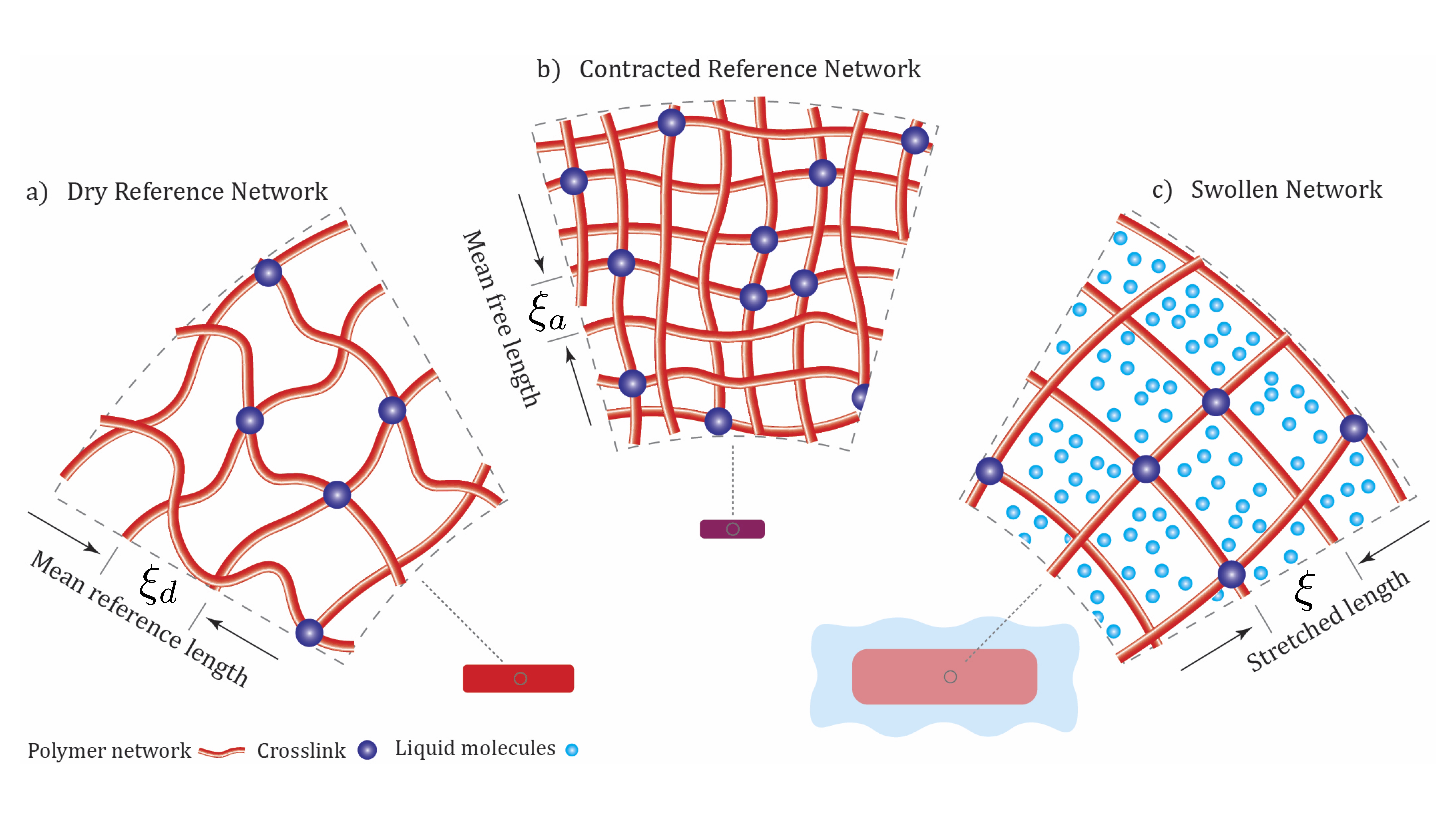
Figure 2: The characteristic states of an active gel: the three cartoons might be considered as representative volume elements. (a) Dry-reference meshwork (red) of size $\xi_{d}$ with crosslinks (blue dots). (b) Dry-contracted meshwork: mesh size $\xi_{a}$ is reduced with respect to $\xi_{d}$, and crosslink density is higher; the polymer chains are considered unstretched. (c) Swollen meshwork: liquid molecules (light blue dots) swell the dry-contracted meshwork: the elastic energy is proportional to the stretch $\xi/\xi_{a}$ between the contracted mesh and the swollen one.

III.1 Model equations under cylindrical symmetry

We exploit the cylindrical symmetry that greatly simplifies the evolution equations of the problem; thus, the reference disc $\mathcal{B}_{d}$ is represented by its vertical cross section $\mathcal{S}_{d}$ spanned by the radial coordinate $r\in(0,R_{d})$ and the vertical one $z\in(0,H_{d})$. With this, the displacement $\mathbf{u}$ has two non trivial components: the radial $u$ and the vertical $w$ component; within the class of remodeling tensors $\mathbf{F}_{a}$ which are cylindrically symmetric, we choose a diagonal one $\mathbf{F}_{a}=\textrm{diag}(\gamma_{r},\gamma_{\theta},\gamma_{z})$.

Hence, the state variables of the problem are reduced to the following six scalar fields: the solvent concentration $c_{d}$, the two displacements $(u,w)$, and the three contractions $(\gamma_{r},\gamma_{\theta},\gamma_{z})$; each field is a function of the coordinates $(r,z)$ and the time $\tau$. Moreover, we assume that the derivatives $u,_{z}$ and $w,_{r}$ can be neglected; it follows that the deformation gradient $\mathbf{F}$ simplifies to $\mathbf{F}=\textrm{diag}(\lambda_{r},\lambda_{\theta},\lambda_{z})$ with the radial, hoop and vertical deformations defined as

$$\lambda_{r}=1+u,_{r},\quad\lambda_{\theta}=1+u/r,\quad\lambda_{z}=1+w,_{z}\,,$$ (III.5)

respectively. Under the symmetry assumption, the volumetric constraint (III.4) takes the form

$$\lambda_{r}\lambda_{\theta}\lambda_{z}=1+\Omega\,c_{d}\,.$$ (III.6)

The active chemo-mechanical state of the active gel is ruled by a set of three balance equations, which can be rationally derived from basic principles [9]: balance of solvent content, of forces, and of remodeling forces. The first two balance equations, under the cylindrical symmetry hypotheses, reduce to the following three scalar equations

$$\begin{array}[]{l}-\dot{c}_{d}=h_{r,r}+\dfrac{h_{r}}{r}+h_{z,z}\,,\\[8.53581pt] s_{r,r}+\dfrac{s_{r}-s_{\theta}}{r}=0\,,\\[8.53581pt] s_{z,z}=0\,.\end{array}$$ (III.7)

In equations (III.7), $h_{r}$ and $h_{z}$ are the radial and vertical components of the solvent flux, whereas $s_{r}$, $s_{\theta}$ and $s_{z}$ are the radial, hoop and vertical components of the reference stress (also called Piola-Kirchhoff stress).
Flux, chemical potential $\mu$ and stresses are related to the stretches $\lambda_{i}$ and the contractions $\gamma_{i}$ ($i=r,\theta,z$), by constitutive equations, whose derivation is fully described in many texts and papers (see [21, 22, 17]). Shortly, liquid transport in the elastic solid is described by a kinetic law, based on the assumption that the liquid molecules diffuse in the gel and the coefficients of diffusion can be different in the radial and vertical direction but independent of the deformation and the concentration. In the end, the liquid flux is related to the gradient of the chemical potential by the following equations

$$h_{r}=-\dfrac{D_{r}\,c_{d}}{R\,T\,\lambda_{r}^{2}}\,\mu,_{r}\quad\textrm{and}\quad h_{z}=-\dfrac{D_{z}\,c_{d}}{R\,T\,\lambda_{z}^{2}}\,\mu,_{z}\,,$$ (III.8)

where $D_{r}$ and $D_{z}$ are the coefficients of diffusion in the radial and vertical direction, $R$ and $T$ are the gas constant and the temperature, respectively, and $\mu$ is the chemical potential of the solvent in the gel:

$$\mu=R\,T\,g(J_{e})+\Omega\,p\,,$$ (III.9)

with

$$g(J_{e})=\left[\log\left(\frac{J_{e}-1}{J_{e}}\right)+\frac{\chi+J_{e}}{J_{e}^{2}}\right]\,,\quad J_{e}=\textrm{det}\,\mathbf{F}_{e}=\frac{J}{J_{a}}\,.$$ (III.10)

Therein, $\Omega$ is the molar volume of the liquid ($[\Omega]=$ m³/mol) and $\chi$ is the non dimensional dis-affinity parameter[15]. The pressure field $p$ is is the Lagrangian multiplier of the constraint $J=J_{a}+\Omega\,c_{d}$ (equation (III.4)). Finally, the stresses are given by

$$s_{r} = G\,\lambda_{r}\,\frac{\gamma_{\theta}\gamma_{z}}{\gamma_{r}}-p\,\lambda_{\theta}\lambda_{z}\,,$$

$$s_{\theta} = G\,\lambda_{\theta}\frac{\gamma_{r}\gamma_{z}}{\gamma_{\theta}}-p\,\lambda_{r}\,\lambda_{z}\,,$$ (III.11)

$$s_{z} = G\,\lambda_{z}\frac{\gamma_{r}\gamma_{\theta}}{\gamma_{z}}-p\,\lambda_{r}\,\lambda_{\theta}\,,$$

where $G$ is the shear modulus of the dry polymer network ($[G]=$J/m³). The (actual) Cauchy stresses are: $\sigma_{r}=s_{r}/\lambda_{\theta}\lambda_{z}$, $\sigma_{\theta}=s_{\theta}/\lambda_{r}\lambda_{z}$ and $\sigma_{z}=s_{z}/\lambda_{\theta}\lambda_{r}$.
The third balance equation, which describes the time evolution of the spontaneous metric delivered by the self-contractions $\gamma_{i}$, reduces to three scalar equations :

$$\begin{array}[]{l}\dfrac{\dot{\gamma}_{r}}{\gamma_{r}}=\dfrac{1}{\eta_{r}}\,(\beta_{r}-E_{r})\,,\\[11.38109pt] \dfrac{\dot{\gamma}_{\theta}}{\gamma_{\theta}}=\dfrac{1}{\eta_{\theta}}\,(\beta_{\theta}-E_{\theta})\,,\\[11.38109pt] \dfrac{\dot{\gamma}_{z}}{\gamma_{z}}=\dfrac{1}{\eta_{z}}\,(\beta_{z}-E_{z})\,.\end{array}$$ (III.12)

The evolution of the self-contractions $\gamma_{i}$ is driven by the differences $(\beta_{i}-E_{i})$ $(i=r,\theta,z)$. Therein, $\beta_{i}$ describes the effect of molecular motors on the mesh, is a control parameter of the model and will be denoted as active stress from now on. On the other hand, the three functions $E_{i}$ are the components of the Eshelby tensor, which is completely determined by the elasto-chemical state of the gel through the Flory-Rehner free-energy and the stress state in the gel as:

$$E_{i}=e_{y}-J\,\sigma_{i}\,,\quad(i=r,\theta,z)$$ (III.13)

with

$$e_{y}=\frac{R\,T}{\Omega}\,J_{a}\,\bigl{(}f_{c}(J_{e})+m\,f_{e}(\mathbf{C}_{e})\bigr{)}-c_{d}\,\mu\,.$$ (III.14)

Therein, $f_{c}$ and $f_{e}$ are the dimensionless mixing and elastic free-energy:

$$f_{c}(J_{e}) = (J_{e}-1)\textrm{log}(1-\frac{1}{J_{e}})+\chi(1-\frac{1}{J_{e}})\,,$$

$$f_{e}(\mathbf{C}_{e}) = \frac{1}{2}(\textrm{tr}\mathbf{C}_{e}-3)\,.$$ (III.15)

So, the equations (III.12)-(III.15) show as the interplay between activity, elasticity and liquid transport depends on the effective stresses $(\beta_{i}-E_{i})$ and on the frictions $(\eta_{r},\eta_{\theta},\eta_{z})$ of the mesh, that is, the resistance of the mesh to remodel, in the three-directions. Frictions bring in the model one or more characteristic times, which affect the mesh remodeling and though it the whole process. Large frictions yield small contraction time rates, under the same effective stresses.
As a first work hypothesis, we assume $\beta_{i}$ to be uniform and isotropic: $\beta_{r}=\beta_{\theta}=\beta_{z}=\beta$. We also assume that the disc is not constrained, nor loaded and, as chemical boundary conditions, we assume that all the disc boundary is permeable and chemical equilibrium holds at the boundary, that is,

$$\mu=\mu_{e}\quad\textrm{on}\quad\partial\mathcal{S}_{d}\,,$$ (III.16)

where $\mu_{e}$ is the difference between the chemical potential of the bath and that of pure water ($\mu_{e}=0$ corresponds to a pure water bath). Finally, the initial conditions for the displacements $u,w$, the concentration $c_{d}$ and the contractions $\gamma_{i}$ ($i=r,\theta,z$) are the following:

$$u=(\lambda_{o}-1)\,r,\quad w=(\lambda_{o}-1)\,z,\quad c_{d}=c_{do},\quad\gamma_{i}=1\,.$$ (III.17)

It means that the deformation $f_{o}$ from the reference region $\mathcal{B}_{d}$ to the initial region $\mathcal{B}_{o}$ is $f_{o}(X)=\lambda_{o}\,X$ for any $X\in\mathcal{B}_{d}$ (see figure 1).

III.2 Details of Finite Element Analysis

Equations (III.6), (III.7) and (III.12), together with the boundary (III.16) and initial (III.17) conditions, are rewritten in a weak form and implemented in the software COMSOL Multiphyisics by using the Weak-Form physics interface. The calculus domain is the rectangular domain $\mathcal{S}_{d}$, which is meshed with triangular elements whose maximum mesh size is $H_{d}/10$, yielding about 200K dofs. Lagrangian polynomials are used as shape functions: polynomials of order 4 for the displacement and the solvent concentration, of order 3 for the volumetric constraint, of order 2 for the boundary conditions (also implemented in weak form) and of order 1 for the remodeling variables. The whole set of coupled equations are solved by using the Newton method with variable damping, as nonlinear solver, the direct solver Pardiso as linear solver is the direct solver Pardiso and the BDF method with order 1-2 as time dependent solver.
As non linear method, it is used the Newton method with variable damping; the linear solver is the direct solver Pardiso, while the time dependent solver uses the BDF method with order 1-2. The time-dependent analysis starts at the initial state $\mathcal{B}_{o}$ and stops at a final equilibrium state $\mathcal{B}_{1}$, which is pre-selected, as we’ll discuss in the next section.

IV Initial and final equilibrium states

The definition of the steady states where contraction dynamics and liquid transport start and finish is an important issue. Here, we get some data on the conditions of the gel discs at the initial and final states in the experiments which have inspired us [5], and reproduce those conditions in the numerical model.
Firstly, we define a steady state as a solution of the balance equations (III.7), (III.12) with $\dot{c}_{d}=0$ and $\dot{\gamma}_{i}=0$ ($i=r,\theta,z$). Such a state is controlled by the pair $(\mu_{e},\beta$), that is by the conditions

$$\mu=\mu_{e}\quad\textrm{and}\quad E_{i}=\beta\quad(i=r,\theta,z).$$ (IV.18)

We study the contraction dynamics between the initial steady state $\mathcal{B}_{o}$, which is represented by a black dot in the diagram of figure 4, and a final steady state $\mathcal{B}_{1}$ (red or blue dots in the diagram of figure 4), corresponding at a time $\tau=\tau_{1}$.
We assume that at the steady states $\mathbf{F}$ and $\mathbf{F}_{a}$ are uniform and spherical, that is $\mathbf{F}=\lambda\,\mathbf{I}$, $\mathbf{F}_{a}=\gamma\,\mathbf{I}$, and that initial and final states are stress-free. With this, equations (III.11), (III.9) and (III.13) deliver a representation form for both the chemical potential and the Eshelby components, in terms of $J_{a}$ and $J$: $\mu=\mu(J/J_{a})=\mu(J_{e})$ and $E_{i}=e_{y}(J_{a},J_{e})$. Equations (IV.18) deliver the relationships between the values of $J_{a}$ and $J$ at the initial and final states and the pair $(\mu_{e},\beta$) which determines those values:

$$\mu_{e}=\mu(J_{e})\quad\textrm{and}\quad\beta=e_{y}(J_{a},J_{e})\,.$$ (IV.19)

In the following, we adopt the following notation: $J_{o}$ and $J_{1}$ denote the values of $J$ at $\mathcal{B}_{o}$ and $\mathcal{B}_{1}$, and the same we do for all the other quantities.
The evolution of the system from $\mathcal{B}_{o}$ to $\mathcal{B}_{1}$, that is, the contraction-liquid transport dynamics, is triggered by defining time laws for the two controls, which have both a characteristic evolution dynamics. For the motors, the characteristic time is dependent on the binding/unbinding kinetics of the motors to the actin filaments. For the chemical potential, the characteristic time reflects the mixing kinetic of possibly free biopolymer chains and the liquid in the bath. We set

$$\begin{array}[]{l}\mu_{e}=\mu_{e}(\tau)=\mu_{o}+(\mu_{1}-\mu_{o})\,\textrm{s}(\tau/\tau_{\mu})\,,\\[5.69054pt] \beta=\beta(\tau)=\beta_{o}+(\beta_{1}-\beta_{o})\,\textrm{s}(\tau/\tau_{\beta})\,,\end{array}$$ (IV.20)

where $\textrm{s}(\cdot)$ is a smoothed step function running from $0$ to $1$ in the interval $(0,1)$ and $\tau_{\mu}$ and $\tau_{\beta}$ (both less than $\tau_{1}$) are the characteristic time of the controls (see Table 1). Thus, $\beta(0)=\beta_{o}$, and $\beta(\tau_{\beta})=\beta_{1}$, and analogously for $\mu_{e}$.

IV.0.1 Material parameters

Table 1: Material and geometrical parameters

shear modulus	$G=135$ Pa
Flory parameter	$\chi=0.4$
water molar volume	$\Omega=1.8e-5$ m3/mol
temperature	$T=293$ K
energy ratio	$m=G\,\Omega/R\,T=1e-6$
diffusivity	$D_{r}=D_{z}=1e-3$ m2/s
friction	$\eta=1e5$ Pa s
initial radius	$R_{o}=1500\,\mu$m
initial swollen volume & stretch ratio	$J_{o}=1000,\,\lambda_{o}=10$
initial aspect ratio	$AR=2\,R_{o}/H_{o}=20\sim 40$
initial thickness	$H_{o}=150\,\mu m\sim 75\,\mu$m
final volume/initial volume	$J_{a1}=0.05$
control time for $\beta$	$\tau_{\beta}=20$ s
control time for $\mu$	$\tau_{\mu}=100$ s

The values assigned to the initial thickness and aspect ratio have been inspired by [5], and the successive parametric analyses always consider values of $AR$ and $H_{o}$ not too far from those ones. Moreover, we considered a highly swollen initial state of the gel, which motivated our choice for the Flory parameter $\chi$ and the shear modulus $G$. Finally, as it has been observed in [5] that the characteristic time of the process is about $200$s, and the characteristic time of the discharge velocity is about $40$s, we tuned the values assigned to the diffusion constants and to the friction in such a way to qualitative match the characteristic times of the dynamics.
Then, we fix the material and geometrical parameters as in Table (1).

IV.0.2 Initial state

We assume a fully swollen state as initial state of the gel, characterized by an unstretched mesh size $\xi_{a}$ equal to the reference mesh size $\xi_{d}$. From an experimental point of view, it means that self contraction and liquid release are going to be initiated; from the modeling point of view, it means that

$$\mu_{eo}=\mu_{o}=0\,\,\textrm{J/mol}\quad\textrm{and}\quad\quad J_{ao}=1\,.$$ (IV.21)

Given these values, we can use equations (IV.19) to get the initial swollen state $J_{o}$ and the value of the active stress $\beta_{o}$ which maintains it: from

$$0=\mu(J/J_{ao})\quad\textrm{and}\quad\beta_{o}=e_{y}(J_{ao},J_{eo})\,,$$ (IV.22)

we get $J_{o}$ and $\beta_{o}$. In particular, being $J_{eo}=J_{o}=\lambda_{o}^{3}$, equation (IV.22)₁ takes the form

$$0=\left[\log\left(\frac{\lambda_{o}^{3}-1}{\lambda_{o}^{3}}\right)+\frac{\chi+\lambda_{o}^{3}}{\lambda_{o}^{6}}\right]+\dfrac{m}{\lambda_{o}}\,,$$ (IV.23)

and can be solved for $\lambda_{o}$, the free-swelling stretch ratio at $\mathcal{B}_{o}$. Therein, $m=G\Omega/R\,T$ is the ratio between the elastic energy and the mixing energy. Equation (IV.22)₂ determines the active stress $\beta_{o}$ (J/m³) corresponding to null self-contraction ($\xi_{a}=\xi_{d}$) and to the free swelling stretch $\lambda_{o}$:

$$\dfrac{\Omega}{R\,T}\beta_{o}=(\lambda_{o}^{3}-1)\left(\dfrac{\lambda_{o}^{3}-1}{\lambda_{o}^{6}}\chi-\dfrac{1}{\lambda_{o}^{3}}\right)+m\left(\dfrac{1}{\lambda_{o}}+\frac{\lambda_{o}^{2}}{2}-\frac{3}{2}\right)\,.$$ (IV.24)

It is worth noting that equation (IV.23) is quite standard in stress-diffusion theories based on a Flory-Rehner thermodynamics [24, 25]; it is easy to verify that, given $\mu_{o}$, the free-swelling stretch $\lambda_{o}$ increases as $m$ decreases, as shown in figure 1 (panel b), where the relation between $\lambda_{o}$ and $m$ has been represented. On the contrary, equation (IV.24) does not belong to standard stress-diffusion theory, and is peculiar of the present augmented model. Figure 1 (panel b) also shows the dependence of $\beta_{o}$ on $\lambda_{o}$.
Finally, equations (IV.23) and (IV.24) deliver the following initial values of $J$, $J_{e}$, $c_{d}$, $p$ and $\beta$:

$$\begin{array}[]{l}J_{eo}=J_{o}=1000\,,\\[5.69054pt] c_{do}=(J_{o}-1)/\Omega=5.5e7\,\,\textrm{mol/m${}^{3}$},\\[5.69054pt] p_{o}=G\,(1/J_{eo})^{1/3}=13.6\,\,\textrm{Pa},\\[5.69054pt] \beta_{o}=e_{y}(1,J_{eo})=-8e7\,\,\textrm{J/m${}^{3}$}.\\[5.69054pt] \end{array}$$ (IV.25)

IV.0.3 Final states

In the experiments, it has been observed the attainment of final steady states, when self contraction and liquid transport stop. In the modeling, we studied the conditions to get final steady states, which are not too far, in terms of some characteristic elements, from those experimental final states.
We considered two different protocols: (a), where only active stresses $\beta\not=\beta_{o}$ drive the active contractions and liquid transport; (b), where bot active stresses $\beta\not=\beta_{o}$ and a change in the chemical potential of the bath from $\mu_{o}$ to $\mu_{e}$ drive the active contractions and liquid transport. In both the protocols, based on the outcomes of the experiments presented in [5], we assume that the unstretched mesh size is contracted by $\xi_{a}/\xi_{d}=J_{a1}^{1/3}\simeq 0.38$ with respect to the dry mesh size, and set the final value $J_{a1}$ of $J_{a}$ in such a way to produce that result: $J_{a1}=(\xi_{a}/\xi_{d})^{3}=0.05$.

Protocol a

Assuming that

$$\mu_{e1}=\mu_{o}=\mu_{1}=0\,\textrm{J/mol}\,,\quad J_{a1}=0.05\,,$$ (IV.26)

equations (IV.19) deliver the final swelling ratio $J_{1}$ and the active stress $\beta_{1}$ needed to maintain it:

$$\mu(J/J_{a1})=0,\,e_{y}(J_{a1},J_{e1})=\beta_{1}\quad\Rightarrow\quad J_{1},\,\,\beta_{1}$$ (IV.27)

Given our parameters, for case (a) we have the following characteristic values of the final state:

$$\begin{array}[]{l}J_{e1}=J_{1}/J_{a1}=J_{eo}=1000\,,\quad J_{1}=50\,,\\[5.69054pt] c_{d1}=(J_{1}-J_{a1})/\Omega=2.8e7\,\,\textrm{mol/m${}^{3}$},\\[5.69054pt] \beta_{1}=e_{y}(J_{a1},J_{e1})=-4e6\,\,\textrm{J/m${}^{3}$}.\\[5.69054pt] \end{array}$$ (IV.28)

It is worth noting that at the initial state, in absence of contraction ($J_{a1}=1$), we get $J_{1}=J_{e1}=1000$, whereas at the final contracted state $\mathcal{B}_{1}$, we get $J_{1}=J_{e1}=50$, that is, a much smaller volume change under the same chemical conditions. It means that the model includes an effective bulk stiffening of the gel due to self-contraction, that is, to motor activity, that has already been recognized as crucial in other works [6].

Protocol b

Typically, in a Lab, the chemical potential of the bath is not controlled. We can suppose it is constant, as in the protocol a) or, as it is possible that some chains of the gel, which are not perfectly cross-linked, are released during the gel contraction, we can assume that it varies [26]. This motivated our choice to follow protocol b), too. We assume that the final swelling ratio $J_{1}$ is half the value of case (a), while $J_{a1}$ is the same as before:

$$J_{1}=25\,,\quad J_{a1}=0.05\,.$$ (IV.29)

Now, equations (IV.19) are used to identify the final chemical potential $\mu_{1}$ and the active stress $\beta_{1}$ needed to maintain this final state:

$$\mu(J_{1}/J_{a1})=\mu_{1},\,e_{y}(J_{a1},J_{e1})=\beta_{1}\,\Rightarrow\,\mu_{1},\,\,\beta_{1}\,.$$ (IV.30)

Given the parameters, for case (b) we have the following characteristic values of the final state:

$$\begin{array}[]{l}J_{e1}=J_{1}/J_{a1}=J_{eo}=500,\\[5.69054pt] p_{1}=G\,(J_{a1}/J_{1})^{1/3}=17.1\,\,\textrm{Pa},\\[5.69054pt] c_{d1}=(J_{1}-J_{a1})/\Omega=1.4e6\,\,\textrm{mol/m${}^{3}$},\\[5.69054pt] \mu_{1}=\mu(J_{a1},J_{e1})=-6.7e-4\,\,\textrm{J/mol},\\[5.69054pt] \beta_{1}=e_{y}(J_{a1},J_{e1})=-4e6\,\,\textrm{J/m${}^{3}$}.\\[5.69054pt] \end{array}$$ (IV.31)

We note that for the two cases, the value of $\beta_{1}$ is the same, but the de-swollen volume $J_{1}$ is quite different ($50$ vs $25$), as for case (b) liquid transport and release is driven by both the mesh contraction and the change in the chemical conditions of the bath, whereas for the case a) only the driving force is only the gel activity.

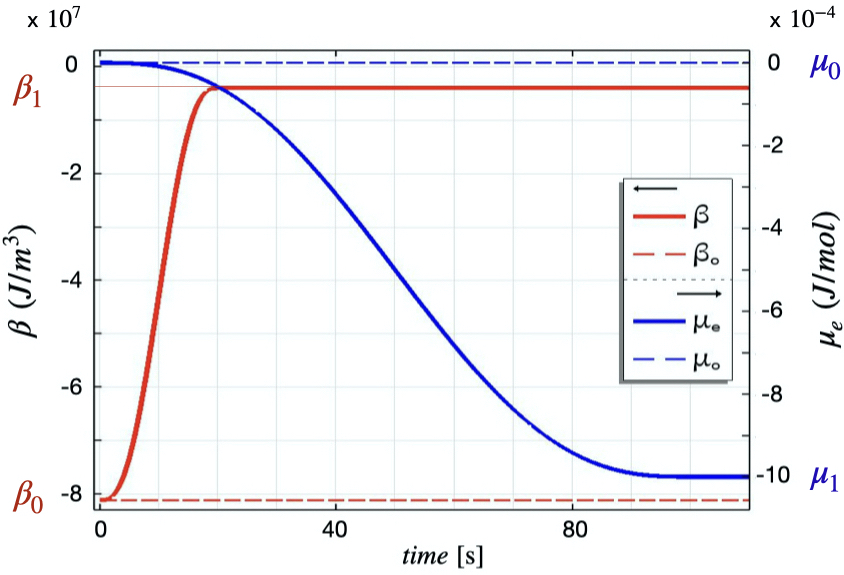
Figure 3: Time laws of the controls $\mu_{e}$ and $\beta$; for both cases (a) and (b), $\beta$ runs from $\beta_{o}=-8\cdot 10^{7}$ J/m³ (at time $\tau=0$ s) to $\beta_{1}=-.4\cdot 10^{7}$ J/m³ (at time $\tau=\tau_{\beta}=20$ s) (dashed & solid red). Case a): $\mu=\mu_{o}=0$ J/mol (at time $\tau=0$ s) (dashed blue). Case b): $\mu$ runs from $\mu_{o}=0$ J/mol to $\mu_{1}=-10^{-3}$ J/mol (at time $\tau=\tau_{\mu}=100$ s) (solid blue). $\beta$ axis at left, $\mu$ axis at right.

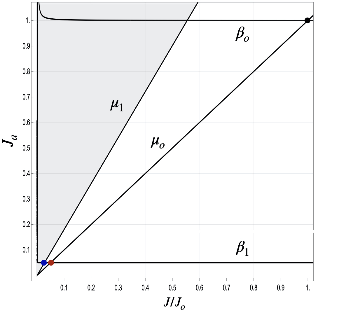
Figure 4: Swelling-contraction diagram $J_{a}$ versus $J/J_{o}$ at equilibrium and stress-free states. The isolines $\mu=\mu_{o}$ and $\mu=\mu_{1}$ are identified by straight lines in this diagram, where the isoline $\beta=\beta_{o}$ and $\beta=\beta_{1}$ are hyperboles. The black dot corresponds to the initial state whereas the red and blue dots corresponds to the final state attained under case a) and b), respectively.

V Contraction dynamics

Our idea is that geometry greatly affect contraction dynamics due to the liquid transport, which has its own characteristic length, diversely from self-contraction dynamics, which don’t have it since motor activity is homogenous across the system.
The key geometrical parameter in a disc is its aspect ratio $AR$; hence, we start investigating the effects of $AR$ on the contraction dynamics with two complementary studies: 1) at fixed radius $R_{o}=1.5$ mm, and varying $H_{o}$; 2) at fixed thickness $H_{o}=0.10$ mm and varying $R_{o}$. The investigated range of parameter $AR$ is described in Table 2: the analysis goes from discs whose AR varies from $20$ (thick discs) to discs of aspect ratio $45$ (thin discs). The study is carried on under the conditions of scenario a).

Table 2: Data about aspect ratios; values of $R_{o}$ and $H_{o}$ are in mm

AR	$R_{o}(H_{o}=0.1)$	$H_{o}(R_{o}=1.5$)
$20$	$1.0$	$0.15$
$25$	$1.25$	$0.12$
$30$	$1.50$	$0.1$
$35$	$1.75$	$0.086$
$40$	$2.0$	$0.075$
$45$	$2.25$	$0.066$

All the experiments start with $J_{o}=1000$, a highly swollen initial state, and $J_{ao}=1$, and evolve towards the new steady values $J_{1}=50$ and $J_{a1}=0.05$. As stated above, these values correspond to a reduction in mesh = $\xi_{a1}/\xi_{ao}=0.05^{1/3}=0.38$, where $\xi_{a1}$ represents the final mesh size at zero stress, see Section IV.

In the regime under study, the system reaches the new equilibrium state at a time $\tau_{1}\simeq 200$ s, that is, we have $\tau_{\beta}<<\tau_{1}$ and dynamics is ruled by the redistribution of water, which has a length scale that is the disc thickness $H_{o}$.
To present our results, we focus on: evolution paths in the plane $(\bar{J},\bar{J}_{a})$; velocities of the lateral boundary of the disc, i.e., radial velocity; radius and thickness reduction. The averages $\bar{J}$ and $\bar{J}_{a}$ of the fields $J(r,z,\tau)$ and $J_{a}(r,z,\tau)$ are introduced to give a global glance at the contraction dynamics and, due to the cylindrical symmetry of the system, are averaged on the cross section $\mathcal{S}_{d}$ of area $R_{d}\cdot H_{d}$. Changes in volume, boundary velocities and changes in radius and thickness have a large effect on the global change in shape of the disc. They are visible in experiments and can be measured, if the appropriate tests are performed. Finally, we analyse the stress state of the gel during the contraction process.

V.1 Dynamics in the plane $(\bar{J},\bar{J}_{a})$

The main features of the contraction dynamics are well represented by the curves $\tau\mapsto(\bar{J}(\tau),\bar{J}_{a}(\tau))$, which are plotted in the plane $(\bar{J},\bar{J}_{a})$. That plane allows us to glance at the quasi-static stress-free path characteristic of an evolution which occurs as a sequence of equilibrium states (straight dashed line). Thinner discs (higher AR) show an evolution in the plane which is closer to the stress-free path. Under the same contraction dynamics, liquid transport is faster for those discs and it allows to quickly recover the original stress-free state. On the contrary, for ticker discs (lower AR) the evolution path is very far from the quasi-static regime: namely, motor-induced contraction is faster than the water trasnport across the gel pores, which makes the gel highly stressed during its evolution.
Figures 5 and 6 show evolution paths for different $AR$ for varying $H_{o}$ at constant $R_{o}$ (figure 5) and varying $R_{o}$ at constant $H_{o}$ (figure 6). In the first case, it is shown as decreasing the thickness $H_{o}$, that is, the characteristic length scale across which water flows, decreases the characteristic time scale of water trasnport (from blue to yellow solid lines). Interestingly, in the second case, that is, changing AR by varying radius under constant thickness, we get a series of fully overlapped curves, so confirming that the important length scale for water exit is $H_{o}$.

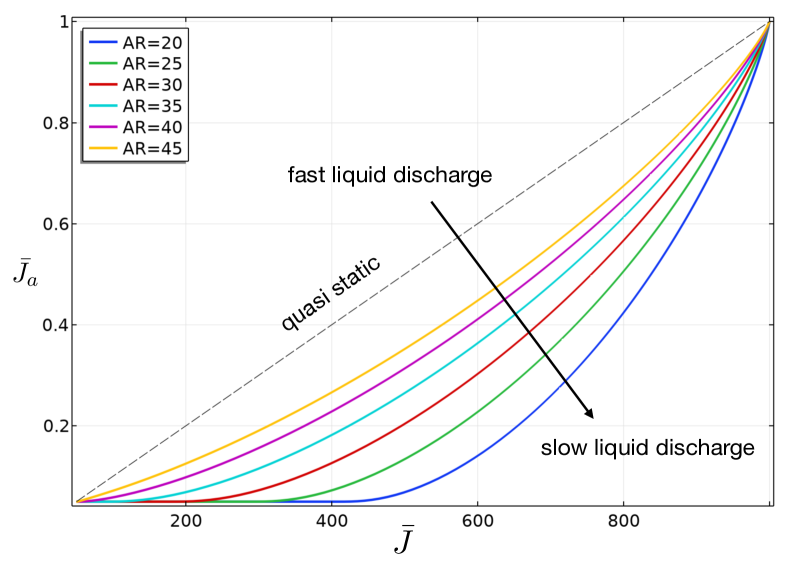
Figure 5: Plane $(\bar{J},\bar{J}_{a})$: evolution path at constant radius $R_{o}=1.5$mm for different values of the aspect ratio AR. Lower AR correspond to evolution path far from equilibrium; higher AR correspond to paths which tend to the quasi-static stress-free path (dashed line).

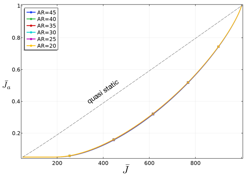
Figure 6: Plane $(\bar{J},\bar{J}_{a})$: evolution path at constant thickness $H_{o}=0.1$mm for different values of the aspect ratio AR. All the paths are superimposed and the master curve is the one corresponding to $AR=30$ in figure 5.

V.2 Gel contraction velocity

Through the aforementioned studies, we investigate also the effects of $AR$ on the radial contraction velocity $\dot{R}(\tau)$ of the lateral boundary of the gel disc.
The radial contraction velocity $\dot{R}(\tau)$ is determined from the average current radius $R(\tau)$

$$R(\tau)=\Lambda_{r}(\tau)R_{d}\quad\textrm{such that}\quad\dot{R}(\tau)=\dot{\Lambda}_{r}(\tau)\,R_{d}\,,$$ (V.32)

where $\Lambda_{r}$ is an average stretch defined as

$$\Lambda_{r}(\tau)=1+\frac{1}{H_{d}}\int_{0}^{H_{d}}\frac{u(R_{d},z,\tau)}{R_{d}}\,dz\,.$$ (V.33)

From (V.32) and (V.33), the radial contraction velocity can be also rewritten as $\dot{R}(\tau)=\dot{\Lambda}_{r}(\tau)\,\dfrac{H_{d}}{2}\,AR$. It is easy to verify that the average stretch $\Lambda_{r}$ also corresponds to the average $\bar{\lambda}_{r}(\tau)$ of the radial deformation $\lambda_{r}(r,z,\tau)$ on the cross section $\mathcal{S}_{d}$ of area $R_{d}\cdot H_{d}$.
The numerical results obtained for a constant radius show that the radial velocity $\dot{R}(\tau)$ is characterized by two time scales, one that characterizes the phase in which the velocity increases and the second of the velocity decrease phase (figure 7). During the growth phase, the curves fit to a linear law, that is, $\dot{R}(\tau)\propto\tau/\tau_{r}$ with $\tau_{r}$ the characteristic time of rising. During the decreasing phase, curves fit to an exponential law $\dot{R}(\tau)\propto v_{max}\exp(-\,\tau/\tau_{decay})$, with $\tau_{decay}$ the characteristic time of decay (see Table 3).

Table 3: Max velocity, peak time, rising time and decay time, for different values of aspect ratio AR

AR	$v_{max}\mu$ m/s	$\tau_{p}$	$\tau_{r}$	$\tau_{\rm{decay}}$
20	$44\mu$m/s	$\simeq 16$ s	$0.22$ s	$13$ s
25	$52\mu$m/s	$\simeq 16$ s	$0.22$ s	$13$ s
30	$74\mu$m/s	$\simeq 17$ s	$0.18$ s	$8$ s
35	$84\mu$m/s	$\simeq 17$ s	$0.14$ s	$3$ s
40	$104\mu$m/s	$\simeq 17$ s	$0.12$ s	$2$ s
45	$111\mu$m/s	$\simeq 17$ s	$0.11$ s	$1.5$ s

The inset in the figure shows that the maximum radial velocity $v_{max}$, attained at peak time $\tau_{p}$, depends on the geometric parameter $R_{o}$ and $H_{o}$.
Actually, the analysis of the equations (V.32) and (V.33) shows that when $AR$ changes with $H_{d}$ (or, equivalently, with $H_{o}$ as the initial free-swelling is homogeneous), with $R_{o}$ constant, the dependence of $\dot{R}$ on $AR$ is also affected by $H_{d}$ and can’t be linear. The same equations show that, for $H_{d}$ constant the dependence of $\dot{R}$ on $AR$ is simply linear. This is what the inset in figure 7 shows for the maximum velocity $v_{max}$, relative to the study at varying radius.
Moreover, we can split the average stretch $\Lambda_{r}$ into an elastic component $\Lambda_{e}$ and an active component $\Lambda_{a}$, related to the analogous multiplicative decomposition of the deformation gradient $\mathbf{F}=\mathbf{F}_{e}\mathbf{F}_{a}$ and of the radial deformation $\lambda_{r}$. Thus, the stretching velocity $\dot{\Lambda}_{r}$ can be additively split in two summands:

$$\dot{R}=(\dot{\Lambda}_{a}\,\Lambda_{e}+\Lambda_{a}\,\dot{\Lambda}_{e})\,R_{d}\,,$$ (V.34)

where $\Lambda_{a}$ and $\Lambda_{e}$ are defined as the average of the active $\gamma_{r}$ and elastic $\lambda_{r}/\gamma_{r}$ radial deformation, with first due to self-contraction and the second driven by liquid transport. Equation (V.34) highlights the existence of two time scales for $\dot{R}$: for $\tau\leq\tau_{\beta}$ the stretching velocity is dominated by the time evolution of $\beta(\tau)$, while for $\tau\geq\tau_{\beta}$ is dominated by solvent release; we have

$$\begin{array}[]{lcll}\dot{R}&\simeq&\dot{\Lambda}_{a}\,\Lambda_{e}\,R_{d}&\textrm{$\tau<\tau_{\beta}$, contraction-dominated regime}\,,\\[5.69054pt] \dot{R}&\simeq&\Lambda_{a}\,\dot{\Lambda}_{e}\,R_{d}&\textrm{$\tau>\tau_{\beta}$, liquid-dominated regime}\,.\end{array}$$ (V.35)

Equation (V.35)₁ shows that during the contraction-dominated regime, that is, for $t<\tau_{\beta}=20$ s, the radial velocity $\dot{R}$ changes with the same rate of $\Lambda_{a}$, which depends on $\beta$, as figures 7 and 8 show (compare the coloured lines with the dashed black line in both figures). On the other side, equation (V.35)₂ shows that during the liquid-dominated regime, that is, for $t>\tau_{\beta}=20$ s, the radial velocity $\dot{R}$ changes with the rate of $\Lambda_{e}$, which depends on liquid transport and on the $AR$ of the disc, as figure 7 shows.
Figures 7 and 8 show also clearly that the maximal velocity is reached when contraction is maximal - as was suggested in [5] (see figure 4f in [5]).

It is worth noting that the remodeling action $\beta$, needed to change the target mesh size, does not further change once it has taken its maximal value. Beyond that, the system evolves towards its steady state by releasing liquid and the steady state is reached when motor applied activity stresses are balanced by network elasticity such that the system reaches a stress free configuration.
It is also worth noting that the difference in the behaviour of the $\dot{R}$ vs time curves in the liquid-dominated regime for $R_{o}$ (figure 7) and $H_{o}$ (figure 8) constant is different as for these geometries thickness is important.

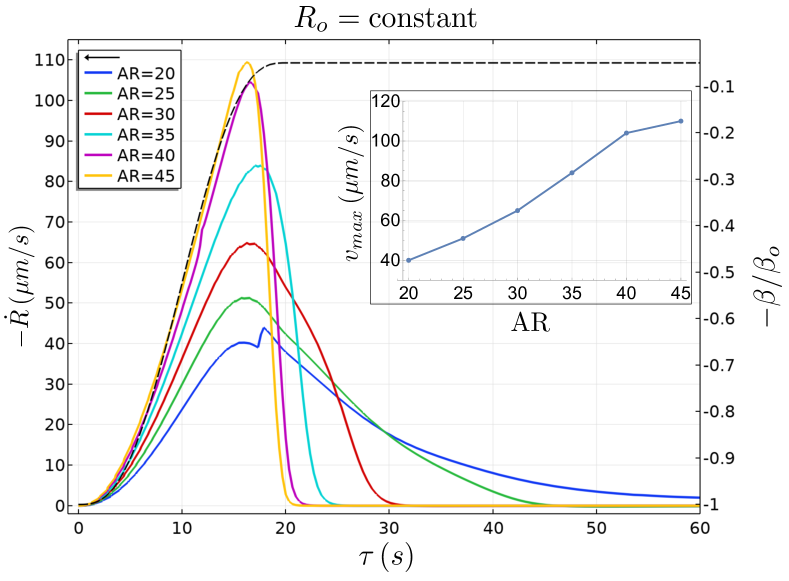
Figure 7: Radial contraction velocity $\dot{R}$ of the lateral boundary of the disc, for different values of $AR$ at constant radius (solid); time evolution of $\beta$ (dashed). The color code is the same as in 5 and 6. The small wiggle in the blue line at $\tau\simeq 17$ s is due to a mechanical buckling: the disc departs from the flat shape, see figure 9, panel (C). Velocity ranges over left vertical axis and $\beta/\beta_{o}$ over right vertical axis.

Figure 8: Radial contraction velocity $\dot{R}$ of the lateral boundary of the disc, for different values of $AR$ at constant thickness (solid) and evolution of $\beta$ (dashed). Color code is the same as in figures 5 and 6. Velocity ranges over left vertical axis and $\beta/\beta_{o}$ over right vertical axis.

V.3 Stress distribution

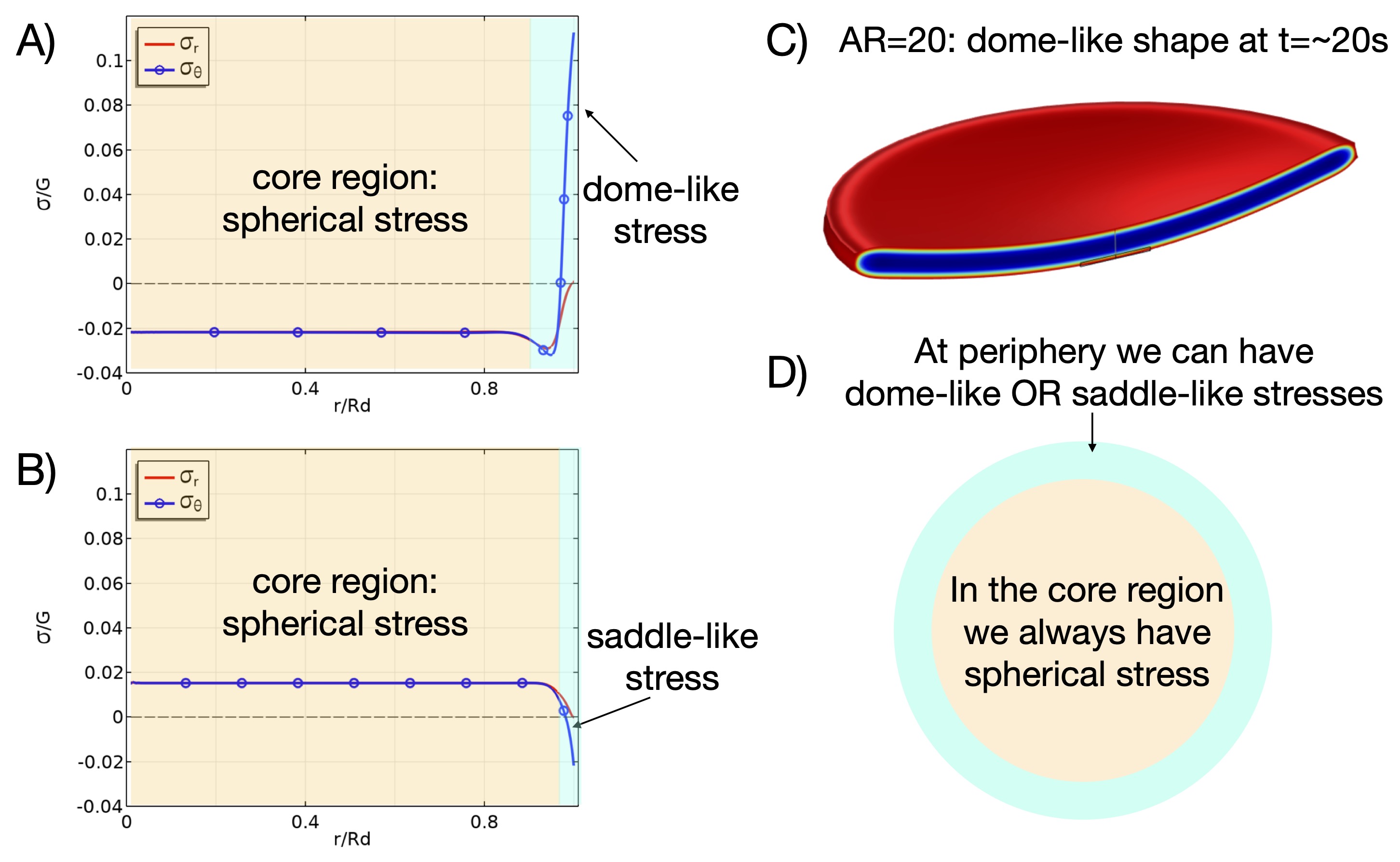
Figure 9: Effect of $AR$ on stress distribution for simulations at constant radius. Panels A) and B) show the radial $\sigma_{r}$ (red) and hoop $\sigma_{\theta}$ (blue) stresses versus the non dimensional radius $r/R_{d}$ at $\tau=20$ s, for $AR=20$ and $AR=45$. A) $AR=20$: the hoop stress is negative in the core (beige) and positive at the periphery (cyan), a typical pattern of frustrated dome-like shape.

Stress analysis in the active disc can be relevant, as it might drive mechanical instability, which lead to a variety of different shapes at the end of the contraction[28, 29, 30, 5]. The analysis of instabilities is beyond the scope of the present work, and will mark our future efforts. However, through the aforementioned studies, we might have interesting clues about shape transitions by investigating the effects of $AR$ on the the evolution of radial and hoop stresses in the disc, which may drive further experiments.

We only report results for the case of constant radius. We compare the stress state in a thick ($AR\simeq 20$) and a thin ($AR\simeq 45$) disc. Panels A) and B) of figure 9 show the existence of two stress patterns: stress is constant in a core region (beige) and varying in a peripheral one (cyan). As bulk contraction $\beta$ is homogeneous and isotropic in the whole disc, these two regions are determined by the dynamics of liquid transport. In particular, the width of the peripheral region is of the order of the thickness because the solvent in this region can escape from both the lateral boundary and the top and bottom surfaces. In contrast, for the solvent in the core the shortest path to exit the gel disc is through the top and bottom surfaces.
In particular, in figure 9, for $AR=20$ we have essentially $\sigma_{r}<0$ along all the radius (see panel A) , and $\sigma_{\theta}$ varying from negative to positive, (see panel A); for $AR=45$ we have $\sigma_{r}>0$ along all the radius (see panel B) and $\sigma_{\theta}$ varying from positive to negative (see panel B). Corresponding to our values of $AR$, we have $H_{\rm{thin}}\simeq 0.04\,R_{d}$ and $H_{\rm{thick}}=0.1\,R_{d}$. The stress distribution for the two cases is typical of that found in frustrated dome-like or saddle-like discs (see figure (9), panels C and D)[28, 29, 30].

That is a preliminary requirement for observing instability patterns which can deliver domes or saddles, depending on other key factors, which are not investigated in the present paper.

V.4 Evolution of aspect ratio during contraction

Finally, the geometry of the gel body suggested to investigate the possibility to have frictions $\eta_{r}$ and $\eta_{\theta}$ in the plane, different from the vertical friction $\eta_{z}$. Frictions are related to the resistances of the mesh to remodel, which can be expected to be different. Our conjecture needs to be validated and the analysis may stimulate further experiments in this direction.
As noted at the end of Section II, the system is controlled by the pair $(\mu_{e},\beta)$, and here we also analyse the combined effects of varying the chemical potential $\mu_{e}$ and active force $\beta$ (protocol b).
We model the motor activity by introducing a uniform and isotropic active stress $\beta$. Nevertheless, during gel contraction, the radial and vertical stretches might differ locally and each one of them can vary in time and space. We use the average values $R(\tau)$ and $H(\tau)$, defined as $H(\tau)=\Lambda_{z}(\tau)\,H_{d}$ with

$$\Lambda_{z}(\tau)=1+\frac{1}{R_{d}}\int_{0}^{R_{d}}\frac{w(r,H_{d},\tau)}{H_{d}}\,dr\,,$$ (V.36)

to describe the change in the aspect ratio of the disc.

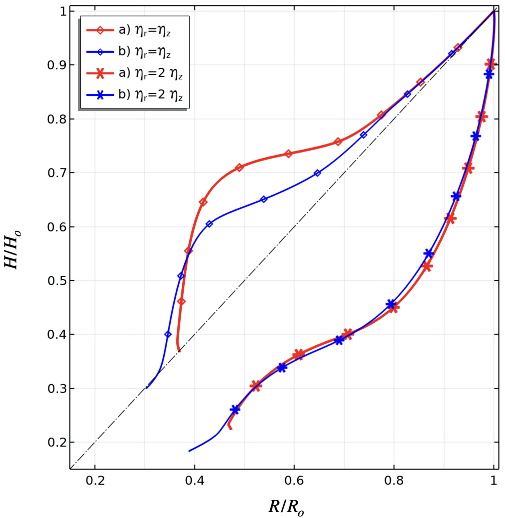
Figure 10: Thickness ratio $H/H_{o}$ versus radius ratio $R/R_{o}$ during contraction for cases a) (red) and b) (blue) with equal friction $\eta_{r}=\eta_{z}$ (diamond) and differential friction $\eta_{r}=2\,\eta_{z}$ (star); $\eta_{r}=10^{5}$ Pa s. Dashed line represents isotropic contractions; with different frictions, the radial and vertical contractions are not isotropic. Disc geometry: $R_{o}=1.5$ mm, $AR=22$.

At any time $\tau$, the ratio ${H}(\tau)/H_{o}$ can be plotted against the ratio ${R}(\tau)/R_{o}$ to illustrate the evolution path of the radial and vertical stretches, that is the curve $\tau\mapsto({R}(\tau)/R_{o},{H}(\tau)/H_{o})$, plotted in the plane $({R}/R_{o},{H}/H_{o})$. In figure 10), the curve has been represented for a disc with $AR=22$ and $R_{o}=1.5$ mm. In that plot, the dashed line represents an isotropic evolution, during which the aspect ratio remains constant during network contraction.
For each of the two analyzed cases a) (red) and b) (blue), we show two curves, one corresponding to equal frictions (diamond), $\eta_{r}=\eta_{\theta}=\eta_{z}$, and the other with different horizontal and vertical frictions (asterisk), $\eta_{r}=\eta_{\theta}=2\,\eta_{z}$. We note that the evolution is very sensitive to friction, while the differences between case a) and b) are less noticeable. For all simulations, the system evolves via a characteristic path. It departs from the isotropic contraction path, but in the case with equal frictions the steady state configuration ends on the dashed line (i.e., on the isotropic path), while the case with different frictions ends far from it. In particular, when $\eta_{r}=\eta_{z}$, the contraction is almost isotropic until $H/H_{o}=R/R_{o}\sim 0.8$; then, radial contraction is faster, and eventually the vertical one becomes faster. When $\eta_{r}=2\,\eta_{z}$, vertical contraction is much faster than the radial one, and the final state is not isotropic.

VI Conclusions and future directions

We discussed the interplay between elasticity, liquid transport and self-contractions in active gel discs from the perspective of continuum mechanics. It has been shown that, even if contraction dynamics doesn’t have a characteristic length, the aspect ratio of active gel discs may greatly affect the changes in shape, due to the dependence of contraction dynamics on liquid transport, which is system-size dependent.
To keep the model easy, the numerical model has been developed under the hypothesis of cylindrical symmetry, which excludes the challenge to observe disc morphings which are not compatible with the cylindrical symmetry. Actually, we are planning to give up the symmetry hypothesis above and investigate the blossom of stresses in the disc, which may drive instability patterns and, consequently, a variety of steady shapes of the gel. It was beyond the scope of the present work and it’ll mark our future efforts.
Giving up the symmetry hypothesis makes also more interesting the identification of the determinants of possible changes in shape, whose control would open to the possibility to get actuators based on self-contractile gels, a promising field which can be set within the framework here presented.