PI-FL: Personalized and Incentivized Federated Learning

Abstract

Personalized FL has been widely used to cater to heterogeneity challenges with non-IID data. A primary obstacle is considering the personalization process from the client’s perspective to preserve their autonomy. Allowing the clients to participate in personalized FL decisions becomes significant due to privacy and security concerns, where the clients may not be at liberty to share private information necessary for producing good quality personalized models. Moreover, clients with high-quality data and resources are reluctant to participate in the FL process without reasonable incentive. In this paper, we propose PI-FL, a one-shot personalization solution complemented by a token-based incentive mechanism that rewards personalized training. PI-FL outperforms other state-of-the-art approaches and can generate good-quality personalized models while respecting clients’ privacy.

1 Introduction

Training high-quality models using traditional distributed machine learning requires massive data transfer from the data sources to a central location. This data transfer raises various communication, computation, and privacy challenges. To this end, Federated Learning (FL) (McMahan et al., 2016) has emerged as a solution to train models at source, which reduces privacy issues and also fulfills the need to create high-quality models. However, the success of FL lies in resolving various new challenges related to heterogeneity, scheduling, and privacy.

Despite its success, FL faces challenges due to the non-IID (non-independently and identically distributed) nature of data. For FL applications, the real-world user data is likely to follow a mixture of multiple distributions (MARFOQ et al., 2021; Ruan & Joe-Wong, 2022). Several research works have focused on training personalized models to overcome data heterogeneity challenges. Instead of training one global model with highly heterogeneous data from all the clients or locally training independent models on each client’s data, training the personalized models is more suitable for independently serving certain clients or groups of clients.

Among personalization research, similarity-based approaches that use clustering of clients at the aggregator (Mansour et al., 2020; Duan et al., 2021; Ruan & Joe-Wong, 2022; Tang et al., 2022) have gained popularity. These works of clustering-based personalization control client selection and training from the aggregator that has limited knowledge of clients’ individual goals or training capacity. This takes away clients’ autonomy to make decisions themselves if they want to bear the cost of training and can also create personalized models that are not aligned with clients’ goals. So it is necessary to reconsider which entity should make the decisions of creating clusters while preserving the autonomy of participating clients.

Existing personalization solutions fulfill the primary goal of overcoming data heterogeneity for specific cases. Nevertheless, they still open the question of how to attract clients to share good quality updates without any reward (Deng et al., 2021; Han et al., 2022; Hu et al., 2022). Training involves computation, communication, as well as privacy costs, and it would be naive to assume that each client would be willing to spend their resources without any measure of benefit being received, which is why clients need to be incentivized to join in training and maximize their profits according to their contributions.

The two challenges of personalizing and incentivizing in FL have always been considered separate problems and dealt with individually. For the practicality of FL, it is logical to create an algorithm design that can cater to both challenges simultaneously. This requires an incentive algorithm that complements personalization in a way that clients are motivated through incentives to produce high-quality personalized models.

To overcome the first challenge of client autonomy, we propose tiering-based personalization according to each client’s preferences. In our work, tier-level models serve as centers and are trained on clients corresponding to that tier. Clients first estimate the importance weights of each tier-level model on their local data. Then guided by the importance weights, clients send their preferences for joining tiers to the aggregator in the form of bids. The aggregator forms tiers for personalized training considering the clients’ bids and their performance history for each tier. To attain personalized models for each client, we do one-shot personalization using tier-level models. It allows independent clients to generate personalize models aligning with the goals that are not directly reflected by their training data and are unknown to the aggregator. This is beneficial, particularly in scenarios where clients may want to use selective data for training while keeping some data private for their personal use due to several reasons such as confidentiality, competitive advantage, data governance, resource limitations, data anonymization or compliance with privacy laws (GDPR (Regulation, 2018), HIPA (Act, 1996)) (Kairouz et al., 2019; Li et al., 2020a). This is also helpful in scenarios where clients may deal with a distribution drift in their data at rapid rates with new incoming data (Liu et al., 2019). With PI-FL, individual clients can attain a personalized model for their new or private data at low computation cost with one-shot personalization.

To resolve the second challenge of incentivizing clients, we propose a token-based incentive scheme as in (Han et al., 2022) that considers each client to have both provider and consumer profiles. As a consumer, the client takes advantage of the final trained personalized model, so it pays the provider to spend resources to train said model in each round. As a provider, the client earns a profit based on its contribution to training the model. The marginal contributions are calculated via a utility function based on Shapley Values  (Shi et al., 2022). Our incentive scheme will reward providers’ participation and contribution of good quality data for training and penalize providers for a contribution reduction.

Lastly, to conjoin personalized and incentivized FL, our incentive algorithm rewards clients on joining tiers where they can provide the most utility. The incentive for each provider’s participation is calculated per tier. If the client enters a tier more similar to its data distribution, it will contribute more to the tier-level model and earn greater profit. In this way, the incentive scheme directly motivates clients to train good quality personalized models and provides rewards accordingly.

Our contributions are: \raisebox{-.9pt} {1}⃝  We present PI-FL, an incentive scheme that complements and rewards personalized learning. \raisebox{-.9pt} {2}⃝  PI-FL provides autonomy to clients for personalized FL and uses the client’s preferences for joining tiers. \raisebox{-.9pt} {3}⃝  To attain personalized models that align with the client’s goals, PI-FL uses a one-shot personalization model that enables clients to create personalized models on new or private data without any chance of data leakage or privacy concerns.

2 Related Work

Personalized FL: FedSoft (Ruan & Joe-Wong, 2022) and (Tang et al., 2021) are probably the closest to our work. FedSoft (Ruan & Joe-Wong, 2022) utilizes soft clustering on the basis of matching data distributions in clients with cluster models. (Tang et al., 2021) and Ditto (Li et al., 2020b) find the optimal personalization-generalization trade-off by solving a bi-level optimization problem. This work incurs clustering overhead at each iteration and does not consider the overlap of distribution between clients wherein each client is restricted to one cluster for each training round. FedGroup (Duan et al., 2021) quantifies the similarities between clients’ gradients by calculating the Euclidean distance of decomposed cosine similarity metric. (Mansour et al., 2020) proposes three approaches for personalization using clustering, data interpolation, and model interpolation. Iterative Federated Clustering Algorithm. IFCA (Ghosh et al., 2020) proposes a framework for the clustering of clients based on the loss values of the gradients. Some other works also propose personalized FL without clustering (Fallah et al., 2020; Kulkarni et al., 2020; Tan et al., 2021; Collins et al., 2021). All of these works lack in providing autonomy to clients in the personalized FL process, they also lack mechanisms to attract good quality clients for participating in the FL process.

Incentivized FL: FAIR (Deng et al., 2021) integrates quality a quality-aware incentive mechanism with model aggregation to improve global model quality and encourage the participation of high-quality learning clients. FedFAIM (Shi et al., 2022) proposes a fairness-based incentive mechanism to prevent free-riding and reward fairness with Shapley value-based client contribution calculation. (Zhang et al., 2021) proposes an approach based on reputation and reverse auction theory which selects and rewards participants by combining the reputation and bids of the participants under a limited budget. (Hu et al., 2022) proposes an approach where clients decide whether to participate based on their own utilities (reward minus cost) modeled as a minority game with incomplete information. Other incentivized FL works include (Zeng et al., 2020; Tang & Wong, 2021; Sun et al., 2021; Gao et al., 2021; Ng et al., 2022). All of these works propose standalone solutions to attract clients, however, they cannot be used as effective solutions to counter the heterogeneity of data in FL to produce good-quality models for individual clients.

In our framework, we use clustering for personalized FL wherein the clusters memberships are changed after every $R$ training rounds. Our work is different from these as we form clear boundaries between multiple cluster models and improve shared learning between cluster similarities through multiple participation at the client level. Our framework also incorporates autonomous client participation with an incentive mechanism that directly motivates personalized training on the basis of Individual Rationality (IR) constraint in game theory. We also provide improved performance in terms of accuracy for personalized and tier-level models.

3 Design

Algorithm 1 PI-FL (Client)

Input: $T_{h}$: Importance weight threshold, $K$: Number of tiers, $M_{k}$: Tier-level model of tier $k\in K$, $D$: Local dataset of client,

Function ClientPreferences($M_{k}$)

2       for  each tier $k\in K$ do

3             for each data point $d\in D$ do

4                   The client computes $\upsilon_{k}$ importance weight of $M_{k}$ model for each data point $d$ via Eqn. 3

5            if $\upsilon_{k}>T_{h}$ then

6                   Client adds tier $k$ to client’s preference bids list $\theta_{i}^{*}$

7            

8      The client generates personalized model $P_{{c}{k}}$ via Eqn. 4 return $\theta_{i}^{*}$

In this section, we describe the design of PI-FL which combines personalization with incentivization using tokens. The idea is to create a democratic incentive system in which all entities benefit proportional to the service they provide and incentivizes personalized training by clients.

For personalization, PI-FL uses a tiering-based approach in which all participating clients within a tier train a tier-level global model. The tier-level global model serves the mutual goals of clients belonging to that tier. Unlike prior works in cluster-based personalization (Duan et al., 2021; Tang et al., 2021; Ruan & Joe-Wong, 2022) in which clients do not have the freedom of choice for joining a particular cluster/tier, we provide autonomy to clients to join tiers in which they can maximize their contributions and, in turn, maximize their rewards.

We assume that each client will look to maximize their profits according to the principle of Individual Rationality (IR) (Kairouz et al., 2019; Li et al., 2020a) and this will lead them to choose tiers in which they can contribute the most for maximum reward.

Algorithm 2 Estimated Shapley value of any client in an FL

0:  Test data $(x_{i},y_{i}),i=1,\ldots,n_{\textrm{test}}$, clients’ local model parameters and aggregation weights, $W_{m},\lambda_{m}$. server’s aggregated model parameter $W_{M}=\sum_{m=1}^{M}\lambda_{m}W_{m}$.

1:  Calculate $\gamma_{M}\overset{\Delta}{=}n_{\textrm{test}}^{-1}\sum_{i=1}^{n_{\textrm{test}}}\nabla_{W}\ell(x_{i},y_{i};W_{M})$

2:  for $k=1,\ldots,M$ do

3:    Calculate $\textsc{shap}(i\rightarrow[M])$ using

$$-\biggl{(}\frac{1}{n_{\textrm{test}}}\sum_{i=1}^{n_{\textrm{test}}}\nabla_{W}\ell(x_{i},y_{i};W_{M})\biggr{)}^{\mathrm{\scriptscriptstyle T}}\lambda_{i}W_{i}$$ (1)

for unnormalized aggregation, or

$$-\biggl{(}\frac{1}{n_{\textrm{test}}}\sum_{i=1}^{n_{\textrm{test}}}\nabla_{W}\ell(x_{i},y_{i};W_{M})\biggr{)}^{\mathrm{\scriptscriptstyle T}}\lambda_{i}(W_{i}-W_{M})$$ (2)

for normalized aggregation.

4:  end for

4:  Obtains all clients’ Shapley values

The aggregator includes three main modules, the profiler, the token manager, and the scheduler.

Algorithm 3 PI-FL (Server)

Input: $R$: Rounds, $P_{r}$: Pre-training rounds, $K$: Number of tiers, $M_{k}$: Tier-level model of tier $k\in K$, $M_{G}$: Global model at aggregator, $N$: Number of clients, $C$: Number of classes in dataset, $\zeta_{a}$: Available Clients, $N_{p}$: Number of clients to select on basis of performance, $N_{r}$: Number of clients to select randomly for each tier, $\zeta_{k}$: Clients selected for training in tier $k\in K$, FedAvg: (McMahan et al., 2016), F1-Scores: (F1-scores, ), sort(): Python 3.7 Timsort implementation (Python, )

for each round $r\in R$ do

10       $\zeta_{k}=SelectClients(r)$ for each tier $k\in K$ for tier $k\in K$ do

11             Server sends tier-level model $M_{k}$ for training to clients in $\zeta_{k}$ Token Manager collects bid payments from all willing clients via Eqn. 6 Token manager updates available tokens for round $r$ via Eqn. 7 $U_{k}\leftarrow$ model updates received from clients in $\zeta_{k}$ $M_{k}=FedAvg(U_{k})$

12      

13 Function SelectClients($r$)

14       if $r=0$ then

15             for $k=1$ to $K$ do

16                   $\zeta_{k}^{*}\leftarrow$ Scheduler randomly assigns clients from $\zeta_{a}$.

17            return $\zeta_{k}^{*}$

18       else if $r>1$ then

19             for $i=1$ to $N$ do

20                   $\theta_{i}\leftarrow ClientPreferences(M_{k})\mid\forall k\in[1,K]$ $//$ from algorithm 1 Server calculates marginal contributions $\psi_{{k}{i}}$ of each client within its tier on basis of Shapley Values via algorithm 2 $\mid\forall k\in[1,K],\forall i\in[1,N]$ $//$Profiler sorts clients on the basis of their marginal contributions and preference bids $S_{c}=sort(\theta_{i},\psi_{{k}{i}})$ for $k=1$ to $K$ do

21                         $\zeta_{k}^{*}\leftarrow$ $N_{p}$ clients selected from $S_{c}$ and $N_{r}$ clients randomly from $\zeta_{a}$ by Scheduler.

22                  

23            return $\zeta_{k}^{*}$

24      

3.1 Profiler

When the FL process starts, the scheduler module forms the initial tiers by randomly assigning clients. Then for each round, the clients train on the tier-level model corresponding to their tier on the client’s local data. After training, these tier-level models are sent to the aggregator for tier-level aggregation. The aggregator aggregates the tier-level models and sends them to the clients.

$$\upsilon_{{c}{k}}=n_{{c}{k}}/n_{k}\in{[0,1]}$$ (3)

The clients calculate the importance weight of each tier-level model on their local dataset as given in Equation 3. Here $\upsilon_{{c}{k}}$ is the normalized sum of correctly predicted data points $n_{{c}{k}}$ on local dataset $D_{c}$ of client $c$ with tier-level model $M_{k}$ where $k\in{K}$. The importance weights are used to generate a one-shot personalized model through the weighted aggregation of tier-level models using Equation 4.

$$P_{{c}{k}}=\sum_{k=1}^{K}\upsilon_{{c}{k}}\times(\omega_{k})$$ (4)

Here the $P_{{c}{k}}$ is the personalized model of client $c$ in tier $k$ and $\omega_{k}$ is the weight vector of $k$ tier-level model. Using this, clients generate good quality one-shot personalized models offline without the need to share their private data.

This resolves challenges related to the autonomy and privacy of clients mentioned in Section 1. The client also uses the generated importance weights and knowledge of received rewards from the previous rounds to make an informed preference decision of joining the next tier for training. It informs the aggregator of its preference by submitting a bid for the tier it wishes to participate in the next training round. This is also shown in Algorithm 1.

To aid in scheduling, the profiler calculates the marginal contributions of each client after every round. The marginal contributions are measured using Shapley Values as shown in Algorithm  2. Shapley Values indicate the data quality of each client and its contribution to the aggregated tier-level global model. This data quality information is sent to the scheduler for scheduling clients in the next training rounds. The calculation of Shapley Values for multiple clients is computationally expensive so we use the approximation function derived in section A.

PI-FL also includes an option to facilitate clients to form well-defined initial tiers. So the clients can avoid the decision-making process in the beginning and streamline their spending when the client contributions and tier distributions are unclear. For this, the profiler and the scheduler module facilitate forming the initial tiers by training for some pre-training rounds. This is done as client contributions and similarity metrics that the clients use among other metrics to make decisions about joining tiers are initially unknown. After pre-training, the profiler calculates per-class F1-Scores $\xi$ of all client local models on an IID test dataset (F1-scores, ). Then the profiler with the help of scheduler tiers clients for the next training round using the K-Means clustering (K-Means, ) algorithm with the $\rho$ most varying F1-scores from $C$ total classes. The Equation 5 shows the calculation of $\rho$ where $C$ is the number of total classes and $N$ is the number of all available clients.

$$\rho=var(\xi_{i})\in[1,C]\mid\forall i\in N$$ (5)

We perform all our evaluations for PI-FL without this feature, but this is an added feature that PI-FL includes for faster convergence and to save clients’ costs. We also realize the constraints in choosing all the clients for training, which is why clients that reply within threshold time in pre-training rounds are used to calculate F1 scores. The remaining clients are considered unexplored and assigned to tiers randomly, they can later settle into appropriate tiers through preference and contributions selection.

3.2 Token Manager

The token manager acts as a bank to orchestrate and keep track of transactions between different clients. At the start of each training round the token manager holds an auction for each tier, and the clients that want to participate in that tier place their bids using tokens. The token manager forwards the list of willing clients to the scheduler to select clients for training. It also deducts payments from the willing clients/consumers as shown in Equation 6. Here $\tau_{i}$ is the tokens owned by client $i$, and $\zeta_{k}$ are the clients willing to participate in the training of tier $k$. The term $\tau_{p}$ in this and the following Equations is the bid amount for a round to be paid by each client.

$$\tau_{i}=\tau_{i}-\tau_{p}\mid i\in\zeta_{k}^{*}$$ (6)

The tokens collected as payments from clients/consumers are then added to the available pool of tokens at the Token Manager as shown in Equation 7. Here $\tau_{{a}{r}}$ are the total available pool of tokens at the Token Manager. The term $N_{p}$ is the number of clients selected on basis of performance and $N_{r}$ is the number of clients selected randomly. The significance of using $N_{p}$ and $N_{r}$ is explained in section 3.3

$$\tau_{{a}{r}}=\tau_{{a}{r}}+(N{p}+N_{r})\times\tau_{p}\mid r\in[1,R]$$ (7)

The token manager also distributes the reimbursement and incentive rewards for each provider/client. Reimbursement is used as a measure to penalize the bad performance of providers/clients. Reimbursement depends on the utility function which is calculated as the percentage of average accuracy improvement of the tier-level model $M_{k}$ compared to the maximum achieved accuracy in past rounds on the local datasets of clients in tier $k$. The utility function is given in Equation 8 and reimbursement calculation is given in Equations 9 and 11, both metrics are calculated at the profiler which assists the token manager in reimbursement.

$$\delta_{util}=\max(0.0,\frac{(Acc_{{k}{r}}-Acc_{{k}{max}})}{Acc_{{k}{max}}})$$ (8)

$$\theta=\frac{\eta\times(\gamma-\min(\gamma,\delta_{util}))}{\gamma}\mid\eta\in[0,1],\gamma\in[0,1]$$ (9)

$$R_{t}=\tau_{{a}{r}}\times\theta\mid\theta\in[0,\gamma]$$ (10)

$$\tau_{i}=\tau_{i}-\tau_{{a}{r}}\times\theta\mid\theta\in[0,\gamma]$$ (11)

$$\forall i\in[1,N],\forall r\in[1,R]$$

In Equation 8, $Acc_{{k}{r}}$ is the tier-level model accuracy in the current round $r$ and $Acc_{{k}{max}}$ is the maximum tier-level model accuracy achieved until the current round $r$. The term $\eta$ in Equation 9 represents the maximum portion of tokens that can be returned and $\gamma$ represents the maximum accuracy improvement that leads to the use of one full token. In Equation 11, $\tau_{{a}{r}}$ are the total number of tokens collected from consumers/clients for $r$ training round. We have used a similar approach to (Han et al., 2022), however, they use the accuracy of the FedAvg model on an IID dataset. It is not practical to assume the presence of an IID dataset that can correspond to the data distribution of clients within a tier which is why we rely on the local dataset of clients within that tier to gather this information.

$$\alpha=sort(\psi_{{k}{i}},\Omega_{{k}{i}})$$ (12)

$$\beta=N_{r}\times\frac{(N_{r}+1)}{2}$$ (13)

$$\tau_{i}=\tau_{i}+\alpha\times\frac{\tau_{{a}{r}}}{\beta}$$ (14)

$$\forall k\in[K],\forall i\in[N],\forall r\in[R]$$

After reimbursement, if there are any tokens left to distribute the token manager uses the marginal contributions calculated by the profiler and sorts providers/clients by their contributions and participation record in Equation 12. Here $\psi_{{k}{i}}$ represents the marginal contributions and $\Omega_{{k}{i}}$ represents the participation records of all clients $N$ in $K$ tiers. The term $\beta$ is a normalizing term from Equation 13 in which $N_{r}$ are the number of providers selected for participation in round $r$. Using the ranks $\alpha$ of providers from sorting and the normalization term $\beta$, the available tokens are distributed between these providers in Equation 14. In Equation 14, $\tau_{i}$ represents the tokens owned by provider/client $i$ and $\tau_{{a}{r}}$ are the tokens available for incentive distribution at the token manager. Through reimbursements to consumers and payments to providers, the Token Manager ensures that each client receives an incentive according to their contributions.

3.3 Scheduler

The scheduler selects clients for each round $r$ by the $SelectClients(r)$ function given in Algorithm 3. The scheduler receives the preference bids $\theta_{i}$ from the token manager, the marginal contributions $\psi_{{k}{i}}$ from the profiler for each client $i\in N$ in tier $k\in K$, where $N$ is the total number of clients and $K$ are the total number of tiers. Using this information scheduler groups clients with similar preference bids and then sorts those clients by their marginal contributions. Then the scheduler selects $N_{p}$ number of clients from the sorted clients and $N_{r}$ number of clients randomly. Both $N_{p}$ and $N_{r}$ are tunable parameters. To reduce bias, a small portion of clients $N_{r}$ are selected randomly which is a technique adopted from previous works (McMahan et al., 2016; Bonawitz et al., 2019; Han et al., 2022; Khan et al., 2022). By grouping clients with similar preferences the scheduler preserves the autonomy of clients mentioned in Section 1 and at the same time it actively prioritizes clients with better data qualities for training in each tier by using their marginal contributions as an indicator of performance.

Thus, PI-FL conjoins incentive and personalized learning by providing contribution-based incentives and doing client selection on the basis of contributions and preference bids to encourage clients in joining tiers where they can contribute the most.

4 Experimental Studies

4.1 Experimental Setup

We use Intel(R) Xeon(R) Gold 6226R CPU @ 2.90GHz instances with 64 cores and NVIDIA GeForce RTX 3070 GPUs for all our experiments. To evaluate the performance of PI-FL we use the CIFAR-10 dataset along with a Synthetic dataset provided in the FedSoft (Ruan & Joe-Wong, 2022) repository. To evaluate PI-FL and related work, we use a simple CNN model that can be trained on client devices with limited system resources to map Cross-Device FL settings (Kairouz et al., 2019). The CNN model has three convolutional layers whose channel sizes are sequentially 32, 64, 64, and two linear layers of sizes 3136 and 128. Our empirical results on these datasets suggest that PI-FL is a promising approach for meeting the practical demands of personalized FL with incentives for Cross-Device FL.

Synthetic Data. We use the same synthetic dataset provided by the FedSoft (Ruan & Joe-Wong, 2022) repository for comparison with our work. The FL system has a total of $N=100$ clients. We use this dataset to demonstrate less heterogeneous and simplistic cases where the data is divided into only 2 distributions $D_{A}$ and $D_{B}$. This experimental setup is duplicated from FedSoft for a fair comparison. We test on different ratio mixtures of $D_{A}$ and $D_{B}$ such as 10:90 and 30:70. In the 10:90 partition, $50$ clients have $90\%$ training data from $D_{A}$ and $10\%$ from $D_{B}$, while the other $50$ have $10\%$ training data from $D_{A}$ and $90\%$ from $D_{B}$. In the 30:70 partition, $50$ clients have $70\%$ training data from $D_{A}$ and $30\%$ from $D_{B}$, while the other $50$ have $30\%$ training data from $D_{A}$ and $70\%$ from $D_{B}$.

CIFAR10. This image dataset has images of dimension 32 × 32 × 3 and 10 output classes. Same as the synthetic dataset we test on different ratio mixtures of $D_{A}$ and $D_{B}$. The only difference is that in 10:90 $50$ clients have $90\%$ training data with $10\%$ testing data from $D_{A}$ and $10\%$ training data with $90\%$ testing data from $D_{B}$ and vice versa. In 30:70 partition, $50$ clients have $70\%$ training data with $30\%$ testing data from $D_{A}$ and $30\%$ training data with $70\%$ testing data from $D_{B}$ and vice versa. In the linear partition, client k has $(0.5+k)\%$ training data from $D_{A}$ and $(99.5-k)\%$ training data from $D_{B}$, and the testing data is $(99.5-k)\%$ from $D_{A}$ and $(0.5+k)\%$ from $D_{B},k=0$, $\cdots$, 99. In the random partition, client k has a random mixture vector generated by dividing the $[0,1]$ range into S segments with $S-1$ points drawn from $Uniform(0,1)$. The testing dataset has the same portion of testing data from the opposite distribution of the training dataset. As in all previous partitions.

In short, unlike the Synthetic dataset, where clients have the same training and testing dataset distributions the training and testing distributions of all CIFAR10 dataset partitions are inverse. We use this dataset to test PI-FL where the aggregator is unaware of the client’s dataset distribution and goals. The reason for preserving the client’s privacy from the FL system is explained in more detail in sections 1 and 4.2. We also use this dataset to analyze linear and random partitions where the number of partitions in the distributions is increased to 100 instead of 2 as in 10:90 and 30:70.

EMNIST. This image dataset has images of dimension 28 x 28 and 52 output classes where 26 classes are lower case letters and 26 classes are upper case letters. We test the dataset on different partitions of 10:90, 30:70, linear and random created in the same way as the CIFAR10 data. The only difference being that $D_{A}$ contains 26 lower case letters and $D_{B}$ has 26 upper case letters.

4.2 Focus of Experimental Study

We use different training and testing data distributions to demonstrate PI-FL’s ability to personalize in case of different goals of clients, which will not be visible to the aggregator server. As previously mentioned in section 1, the difference can arise due to multiple reasons, such as a drift in the client’s distribution of data with time or even for privacy and security reasons where the client may not be willing to share a portion of their private data at all with the server and keep it limited to personal use only. In such scenarios, producing quality personalized models and managing incentives becomes a non-trivial task.

Since we expect that initially tier-level models will be deployed to new users, we analyze their test accuracy on holdout datasets sampled from the corresponding tier distributions ($D_{A}$ and $D_{B}$). We also calculate the personalized model test accuracy for each client on the client’s local test data to get a measure of the quality of personalized models on the client side.

4.3 Personalization experimental study

Table 1: Test accuracy for PI-FL and FedSoft on Synthetic Dataset

	PI-FL				FedSoft
	10:90		30:70		10:90		30:70
	c0	c1	c0	c1	c0	c1	c0	c1
$\theta_{0}$	$63.68\%$	$41.26\%$	$58.02\%$	$57.71\%$	$48.90\%$	$49.50\%$	$47.99\%$	$48.36\%$
$\theta_{1}$	$43.71\%$	$63.82\%$	$58.58\%$	$58.47\%$	$50.70\%$	$49.60\%$	$49.99\%$	$50.04\%$

4.3.1 Results on Synthetic data.

For Synthetic Data, we use the learning rate $\eta=0.01$, batch size = 128 and perform training for 300 rounds with both PI-FL and FedSoft. For testing this setting to compare with FedSoft, we use the same testbed as in the original paper. These experiments will showcase the performance of PI-FL in comparison with other works in different heterogeneous settings with augmented data.

Table 2: Test accuracy for PI-FL on CIFAR10 Dataset

	10:90		30:70		linear		random
	c0	c1	c0	c1	c0	c1	c0	c1
$\theta_{0}$	$62.78\%$	$2.56\%$	$53.28\%$	$34.32\%$	$61.66\%$	$12.08\%$	$66.9\%$	$19.48\%$
$\theta_{1}$	$1.5\%$	$70.96\%$	$30.38\%$	$61.94\%$	$30.94\%$	$59.44\%$	$19.12\%$	$58.42\%$

Table 3: Test accuracy for PI-FL and FedSoft on CIFAR10 Dataset

	10:90		30:70		linear		random
	c0	c1	c0	c1	c0	c1	c0	c1
PI-FL	$62.68\%(0)$	$70.96\%(1)$	$53.28\%(0)$	$61.94\%(1)$	$61.66\%(0)$	$59.44\%(1)$	$66.90\%(0)$	$58.42\%(1)$
FedSoft	$32.50\%(0)$	$38.62\%(1)$	$20.28\%(0)$	$23.58\%(0)$	$34.42\%(1)$	$49.62\%(1)$	$21.62\%(1)$	$33.12\%(1)$

Table 1 shows the test accuracy for the 10:90 and 30:70 partitions with PI-FL. Here $\theta_{0}$ represents the distribution $D_{A}$ and $\theta_{1}$ represents the distribution $D_{B}$. The tiers are represented with $c$ along with the tier number. We see that PI-FL performs better for the 10:90 partition where each tier is able to dominate one of the distributions.

The accuracies under the 10:90 partition show that clients that have a greater portion of data from $\theta_{0}$ prefer to train in tier $c_{0}$ whereas clients that have a greater portion of data from $\theta_{1}$ prefer to train in tier $c_{1}$. The tier $c_{0}$ achieves $63.68\%$ accuracy while $c_{1}$ has an accuracy of $63.82\%$. As expected and showcased in previous works (Ruan & Joe-Wong, 2022) the performance for 30:70 is not as good as it is a less heterogeneous partition than 10:90 which is why neither tier dominates a single distribution.

Compared to PI-FL, FedSoft tier-level models accuracies for the 10:90 partition are $50.8\%$ and $49.3\%$. It is worth noting that FedSoft is unable to cater to different partitions of data through its clustering mechanism and the performance gets adversely impacted by increased heterogeneity. Furthermore, Table 1 highlights that tier-level models in FedSoft are unable to dominate a single distribution of data.

For the 30:70 partition with FedSoft, both tier-level models $c0$ and $c1$ perform well on $\theta_{1}$ which means that the clients with different distributions are not being clearly differentiated for training with different tiers. Another thing to note here is that the tier-level models $c0$ and $c1$ have similar performance with either distribution ($\theta_{0}$ and $\theta_{1}$), this is because FedSoft promotes personalizing models when clients have a greater percentage of shared data. This generates tier-level models that are unable to represent a single distribution and do not perform as well as PI-FL with non-IID data.

Figure 1 shows the empirical Cumulative Distribution Function (CDF) plot of personalized accuracies for all clients with the Synthetic data. The average personalized accuracy for the 10:90 and 30:70 partitions are $45.9\%$ and $54.9\%$ respectively. Compared to this, FedSoft achieves $44.75\%$ and $43.69\%$ respectively. An important thing to note here is that in the Synthetic data, the distribution of training and testing data is the same. So the aggregator can use the training data performance as an indicator of the client’s goals for generating personalized models. However, as we see in Figure 1, PI-FL is able to generate personalized models with increased test accuracy than FedSoft regardless of the aggregator’s scope of knowledge. This is made possible by the autonomy that PI-FL provides to clients to join tiers of their own choice which creates accurate tiers and ultimately leads to good-quality personalized models.

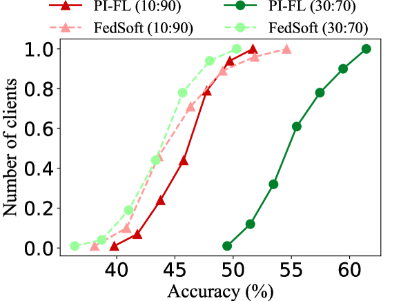
Figure 1: CDF of clients’ personalized model test accuracy for PI-FL and FedSoft on Synthetic Data

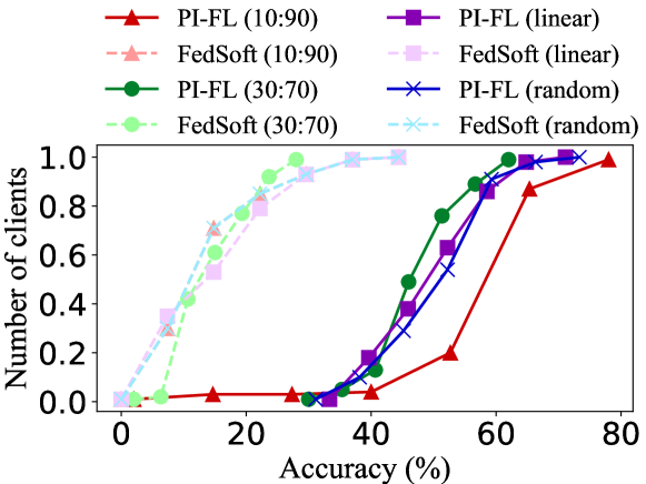
Figure 2: CDF of clients’ personalized model test accuracy for PI-FL and FedSoft on CIFAR10 Dataset

4.3.2 Results on CIFAR10 data.

For evaluation with CIFAR10 Data, we use the same configurations as in subsection 4.3.1. We perform training for 500 rounds with both PI-FL and FedSoft. The Table 2 shows the tier-level model test accuracies for PI-FL with CIFAR10 data. PI-FL accurately differentiates between clients of different distributions. This is visible by the accuracy difference of each tier-level model on different distributions. For example on the 10:90 partition $c1$ model has a $70.96\%$ accuracy on the $\theta_{1}$ distribution and has $2.56\%$ accuracy on $\theta_{0}$ which indicates that tier-level model $c1$ trains with clients that have the majority of their training data from $\theta_{1}$. Similarly, $c0$ trains with clients that have their majority of training data from $\theta_{0}$ and has an accuracy of $62.78\%$.

Table 4: Test accuracy of ablation study with Incentive (PI-FL (I)) and without incentive (PI-FL (NI)).

	10:90		30:70		linear		random
	c0	c1	c0	c1	c0	c1	c0	c1
PI-FL (I)	$58.62\%(0)$	$67.4\%(1)$	$51.12\%(0)$	$64.06\%(1)$	$66.2\%(0)$	$57.02\%(1)$	$64.54\%(0)$	$56.86\%(1)$
PI-FL (NI)	$49.92\%(1)$	$52.8\%(1)$	$48.9\%(0)$	$44.44\%(1)$	$50.82\%(1)$	$45.92\%(1)$	$57.42\%(1)$	$46.76\%(1)$

Table 3 shows the tier-level model accuracy comparison of PI-FL and FedSoft. The number inside the parenthesis along with accuracy shows the distribution for which the tier-level model performs best. For example, for the linear partition, PI-FL $c0$ tier-level model has an accuracy of $61.66\%$ for distribution $\theta_{0}$ and $59.44\%$ accuracy for distribution $\theta_{1}$. For the linear partition with FedSoft, both $c0$ and $c1$ perform best on only one distribution $\theta_{1}$ with accuracy $34.42\%$ and $49.62\%$. Pi-FL outperforms FedSoft in terms of accuracy for each partition and is able to distinguish between different distributions accurately.

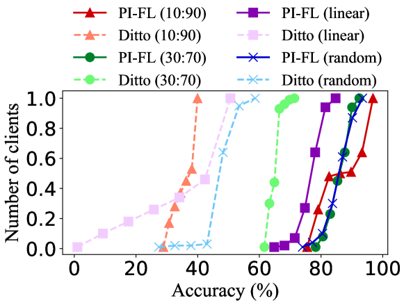
Figure 3: CDF of clients’ personalized model test accuracy for PI-FL and Ditto on EMNIST Dataset

4.3.3 Results on EMNIST Dataset

Since Ditto is not a clustering-based algorithm, we only compare the test accuracy of personalized models on the EMNIST dataset for PI-FL and Ditto in Figure 3. PI-FL outperforms Ditto significantly, especially for highly heterogeneous data partitions such as 10:90 and linear. The reason for this performance improvement is that, unlike Ditto, PI-FL provides autonomy to clients to personalize according to their own goals. With Ditto, the goal of each client which consists of their private data is hidden from the aggregator server which affects the quality of personalized models.

4.3.4 Ablatian study with Incentive in PI-FL

We perform an ablation study with the incentive component of PI-FL where we repeat the experiments from section 4.3.2 on the CIFAR10 dataset for 200 rounds using the same settings and configurations, the only difference being that clients do not consider maximizing their incentive while sending preference bids. Instead, clients send preference bids with random tier choices to the scheduler.

Table 4 shows the test accuracies of the tier-level models. PI-FL(I) indicates that incentives are enabled and PI-F(NI) shows the accuracies when incentives are disabled. In general PI-FL(I) outperforms PI-FL(NI) in terms of test accuracy for all partitions. The important point to note here is that the incentive mechanism in PI-FL directly motivates clients to join tiers in which they can have the most contribution. This results in accurate tiering based on client data distributions and good-quality personalized models. This is indicated by the performance of PI-FL(NI), i.e without incentive, tier-level models are unable to dominate a single distribution and only perform well for a single distribution for all partitions except 30:70. Compared to this, in PI-FL(I) each tier-level model dominates and performs well for their distribution.

We also show a CDF of personalized test accuracies in Figure 4. It can be observed that except for the 30:70 partition, the personalized test accuracies for all other partitions are higher with the incentive enabled which means incentivizing also has a direct impact on the personalized model quality. We argue that the test accuracy for 30:70 is low in this case because it is a less heterogeneous data case and PI-FL performs best in cases where data is highly heterogeneous and requires personalized learning.

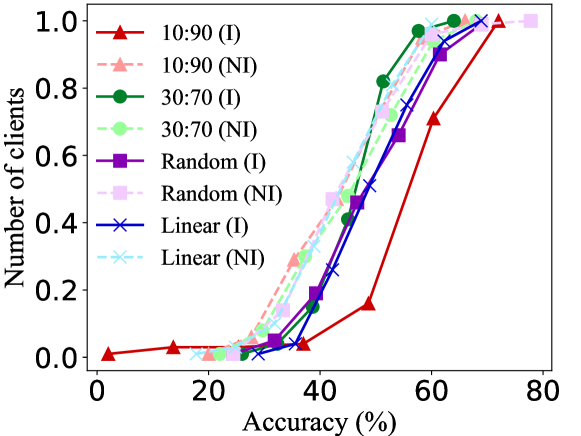
Figure 4: CDF of clients’ personalized model test accuracy for PI-FL with and without incentive on CIFAR10 Dataset. (I) indicates PI-FL with incentives enabled and (NI) indicates incentives disabled

5 Concluding Remarks

In this paper, we proposed PI-FL to address the challenges of heterogeneity, privacy and accessibility in FL. Unlike prior works that consider incentivizing and personalization as separate problems and propose standalone solutions, the key idea for this paper was to conjoin both mechanisms in a way that they complement each other. PI-FL connects a one-shot tiering-based personalized FL algorithm with a token-based incentive mechanism that produces good quality offline personalized models while preserving clients’ private data. Extensive empirical evaluation shows its promising performance compared to other state-of-the-art works.

Appendix A Evaluating Client Contribution using Shapley value

Notation: Let $[M]$ denote the set $\{1,\ldots,M\}$, and $A-B$ the set of elements in $A$ but not in $B$. In this section, $[M]$ denotes all the agents that participate in the coalition. We will consider those not participating in the near future.

We aim to look for a reasonable way to quantify the amount of each client’s contribution in a round. Suppose at any particular round, the server obtains an aggregated model with parameter

$$W_{[M]}\overset{\Delta}{=}\sum_{m\in[M]}\lambda_{m}W_{m},$$ (15)

where $\lambda_{m}$ is the weight (usually $n_{m}/n$ where $n_{m}$ and $n$ are sample sizes of client $m$ and all clients, respectively), and $W_{m}$ is the locally updated model of client $m$.

The prediction loss of the model with parameter $W$, denoted by $\mathcal{L}(W)$, is approximated by

$$\mathcal{L}(W)\approx\frac{1}{n_{\textrm{test}}}\sum_{i=1}^{n_{\textrm{test}}}\ell(x_{i},y_{i};W),$$ (16)

where $(x_{i},y_{i})$, $i=1,\ldots,n_{\textrm{test}}$, is a set of test data. At round $t$, we define the value function of a set of agents $C$ based on how much their contributed model, denoted by $W_{C}$, has decreased the loss of the earlier model, denoted by $W_{t-1}$, namely

$$v_{t}(C)\overset{\Delta}{=}\mathcal{L}(W_{t-1})-\mathcal{L}(W_{C}),$$ (17)

so that the larger the better. When there is no ambiguity, we simply write $v_{t}$ as $v$. It is worth noting that $v$ is a function of the set while $\mathcal{L}$ is a function of the parameter. Once $C$ is realized, $W_{C}$ will become $W_{t}$ for the next round.

Recall that the original Shapley value of agent $m$ given a set of agents $A$ and a value function $v$ is defined by

$$\sum_{S\in A-\{m\}}\frac{|S|!(|A|-1-|S|)!}{|A|!}(v(\{S\cup\{m\}\})-v(S)),$$ (18)

whose sum over all agents is equal to $v(A)-v(\emptyset)$. Here, $\emptyset$ represents the baseline coalition scenario, from which the contribution of each agent is quantified. To highlight the dependency on baseline, we use $B$ to denote the baseline and rewrite (18) as

$$\textsc{shap}(m\rightarrow A\mid B)$$ (19)

$$\overset{\Delta}{=}\sum_{S\in A-\{m\}}\frac{|S|!(|A|-1-|S|)!}{|A|!}(v(\{S\cup\{m\}\}\mid B)-v(S\mid B)),$$ (20)

where $v(S\mid B)$ means the value of $S$ conditional on the baseline $B$. In our scenario, $B$ means the set of agents that are already in coalition and thus

$$v(S\mid B)\overset{\Delta}{=}v(S\cup B).$$ (21)

Let us consider the baseline as $B\overset{\Delta}{=}[M]-\{i,j\}$. The corresponding baseline model will be

$$\textrm{unnormalized version:}\quad W_{[M]-\{i,j\}}\overset{\Delta}{=}\sum_{m\in[M]-\{i,j\}}\lambda_{m}W_{m},$$ (22)

$$\textrm{normalized version:}\quad W_{[M]-\{i,j\}}^{*}\overset{\Delta}{=}\frac{1}{\sum_{m\in[M]-\{i,j\}}\lambda_{m}}\sum_{m\in[M]-\{i,j\}}\lambda_{m}W_{m}.$$ (23)

We consider an unnormalized version for brevity. The additional value by introducing $i,j$ is

$$v(\{i,j\}\mid[M]-\{i,j\})-v(\emptyset\mid[M]-\{i,j\})$$ (24)

$$\begin{subarray}{c}\textrm{use}(\ref{eq_value})\end{subarray}=v([M])-v([M]-\{i,j\})$$ (25)

$$\begin{subarray}{c}\textrm{use}(\ref{eq_value2})\textrm{ and recall }(\ref{eq_thetaM})and(\ref{eq_thetaij})\end{subarray}=\mathcal{L}(W_{[M]-\{i,j\}})-\mathcal{L}(W_{M})$$ (26)

$$=\frac{1}{n_{\textrm{test}}}\sum_{i=1}^{n_{\textrm{test}}}\{\ell(x_{i},y_{i};W_{M})-\ell(x_{i},y_{i};W_{[M]-\{i,j\}})\}$$ (27)

$$\approx\frac{1}{n_{\textrm{test}}}\sum_{i=1}^{n_{\textrm{test}}}\nabla_{W}\ell(x_{i},y_{i};W_{M})^{\mathrm{\scriptscriptstyle T}}(W_{[M]-\{i,j\}}-W_{M})$$ (28)

$$=-\biggl{(}\frac{1}{n_{\textrm{test}}}\sum_{i=1}^{n_{\textrm{test}}}\nabla_{W}\ell(x_{i},y_{i};W_{M})\biggr{)}^{\mathrm{\scriptscriptstyle T}}(\lambda_{i}W_{i}+\lambda_{j}W_{j}).$$ (29)

Next, we calculate how much agent $i$ should be attributed to the above gain that is achieved by $i,j$ jointly. To that end, we calculate the Shapley value of agent $i$ conditional on that agents in $[M]-\{i,j\}$ already participate, namely

$$\textsc{shap}(i\rightarrow\{i,j\}\mid[M]-\{i,j\})$$ (30)

$$\begin{subarray}{c}\textrm{recall }(\ref{eq_Shapley2})\end{subarray}=\sum_{S\in\{j\}}\frac{|S|!(1-|S|)!}{2!}\biggl{(}v\biggl{(}S\cup\{i\}\cup([M]-\{i,j\})\biggr{)}$$

$$\hskip 128.0374pt-v\biggl{(}S\cup([M]-\{i,j\})\biggr{)}\biggr{)}$$ (31)

$$=\frac{1}{2}\biggl{(}v([M])-v([M]-\{j\})+v([M]-\{i\})-v([M]-\{i,j\})\biggr{)}$$ (32)

$$=\frac{1}{2}\biggl{(}-\mathcal{L}(W_{M})+\mathcal{L}(W_{M,-i})-\mathcal{L}(W_{M,-j})+\mathcal{L}(W_{M,-ij})\biggr{)}$$ (33)

$$=\frac{1}{2}\biggl{(}-\mathcal{L}(W_{M})+\mathcal{L}(W_{M,-i})+\mathcal{L}(W_{M})-\mathcal{L}(W_{M,-j})+\mathcal{L}(W_{M,-ij})-\mathcal{L}(W_{M})\biggr{)}$$ (34)

$$\begin{subarray}{c}\textrm{use }(\ref{eq_4})-(\ref{eq_3})\textrm{ and alike }\end{subarray}\approx-\frac{1}{2}\biggl{(}\frac{1}{n_{\textrm{test}}}\sum_{i=1}^{n_{\textrm{test}}}\nabla_{W}\ell(x_{i},y_{i};W_{M})\biggr{)}^{\mathrm{\scriptscriptstyle T}}(\lambda_{i}W_{i}-\lambda_{j}W_{j}+\lambda_{i}W_{i}+\lambda_{j}W_{j})$$

$$=-\biggl{(}\frac{1}{n_{\textrm{test}}}\sum_{i=1}^{n_{\textrm{test}}}\nabla_{W}\ell(x_{i},y_{i};W_{M})\biggr{)}^{\mathrm{\scriptscriptstyle T}}\lambda_{i}W_{i}$$ (35)

which, interestingly, does not depend on $j$. As such, we use this to calculate the Shapley value of client $i$, denoted by

$$\textsc{shap}(i\rightarrow[M])\overset{\Delta}{=}-\biggl{(}\frac{1}{n_{\textrm{test}}}\sum_{i=1}^{n_{\textrm{test}}}\nabla_{W}\ell(x_{i},y_{i};W_{M})\biggr{)}^{\mathrm{\scriptscriptstyle T}}\lambda_{i}W_{i}.$$ (36)

From Equalities (29) and (35), we can verify that

$$v(\{i,j\}\mid[M]-\{i,j\})-v(\emptyset\mid[M]-\{i,j\})=\textsc{shap}(i\rightarrow[M])+\textsc{shap}(j\rightarrow[M])$$

Remark A.1 (Intuitions).

Intuitively, our derived Shapley value of client $i$ in (35) can be regarded as the model’s marginal reduction of the test loss by introducing client $i$. To see that, consider the following approximation based on first-order Taylor expansion:

$$\frac{1}{n_{\textrm{test}}}\sum_{i=1}^{n_{\textrm{test}}}\ell(x_{i},y_{i};W_{M}-\Delta)-\frac{1}{n_{\textrm{test}}}\sum_{i=1}^{n_{\textrm{test}}}\ell(x_{i},y_{i};W_{M}W)$$ (37)

$$\approx-\biggl{(}\frac{1}{n_{\textrm{test}}}\sum_{i=1}^{n_{\textrm{test}}}\nabla_{W}\ell(x_{i},y_{i};W_{M})\biggr{)}^{\mathrm{\scriptscriptstyle T}}\Delta W,$$ (38)

which becomes the term in (35) when $\Delta W\overset{\Delta}{=}\lambda_{i}W_{i}$. The above quantity approximates the amount of client $i$’s contribution to decreasing the test loss of the server’s aggregated model, the larger the better.

Remark A.2 (Normalized counterpart).

Suppose we use the normalized version introduced in (23) when considering the baseline without clients $i,j$. Thus,

$$W^{*}_{[M]-\{i,j\}} =\frac{W_{M}-\lambda_{i}W_{i}-\lambda_{j}W_{j}}{\sum_{m\in[M]-\{i,j\}}\lambda_{m}}$$ (39)

$$=W_{M}+\frac{(\lambda_{i}+\lambda_{j})W_{M}-\lambda_{i}W_{i}-\lambda_{j}W_{j}}{\sum_{m\in[M]-\{i,j\}}\lambda_{m}}$$ (40)

$$=W_{M}-\frac{\lambda_{i}(W_{i}-W_{M})+\lambda_{j}(W_{j}-W_{M})}{1-(\lambda_{i}+\lambda_{j})}.$$ (41)

Similarly, we have

$$W^{*}_{[M]-\{i\}} =W_{M}-\frac{\lambda_{i}(W_{i}-W_{M})}{1-\lambda_{i}}.$$ (42)

Bringing the above formula into (34), we have

$$\textsc{shap}(i\rightarrow\{i,j\}\mid[M]-\{i,j\})$$ (43)

$$=\frac{1}{2}\biggl{(}-\mathcal{L}(W_{M})+\mathcal{L}(W_{M,-i})+\mathcal{L}(W_{M})-\mathcal{L}(W_{M,-j})+\mathcal{L}(W_{M,-ij})-\mathcal{L}(W_{M})\biggr{)}$$ (44)

$$\approx-\biggl{(}\frac{1}{n_{\textrm{test}}}\sum_{i=1}^{n_{\textrm{test}}}\nabla_{W}\ell(x_{i},y_{i};W_{M})\biggr{)}^{\mathrm{\scriptscriptstyle T}}\Delta W^{*}\textrm{ where }$$ (45)

$$2\Delta W^{*}\overset{\Delta}{=}\frac{\lambda_{i}(W_{i}-W_{M})}{1-\lambda_{i}}-\frac{\lambda_{j}(W_{j}-W_{M})}{1-\lambda_{j}}+\frac{\lambda_{i}(W_{i}-W_{M})+\lambda_{j}(W_{j}-W_{M})}{1-(\lambda_{i}+\lambda_{j})}.$$ (46)

$$\approx 2\lambda_{i}(W_{i}-W_{M})$$ (47)

assuming small $\lambda_{i}$ and $\lambda_{j}$. Therefore, under normalization we have

$$\textsc{shap}(i\rightarrow\{i,j\}\mid[M]-\{i,j\})\approx-\biggl{(}\frac{1}{n_{\textrm{test}}}\sum_{i=1}^{n_{\textrm{test}}}\nabla_{W}\ell(x_{i},y_{i};W_{M})\biggr{)}^{\mathrm{\scriptscriptstyle T}}\lambda_{i}(W_{i}-W_{M}).$$ (48)

The intuition is the same as Remark A.1 except that the server model with client $i$ satisfies

$$\textrm{unnormalized version}:\quad W_{[M]-\{i\}}=W_{M}-\lambda_{i}W_{i}.$$ (49)

$$\textrm{normalized version}:\quad W_{[M]-\{i\}}\approx W_{M}-\lambda_{i}(W_{i}-W_{M}).$$ (50)

Appendix B Multiple distribution Results

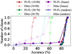
Figure 5: CDF of clients’ personalized model test accuracy for PI-FL and Ditto on 4 and more distributions with EMNIST Dataset

PI-FL outperforms other FL personalization algorithms in heterogeneous cases when the clients and dataset are divided between 2 distributions (DA & DB). To analyze the reliability of PI-FL it is also evaluated in highly heterogeneous conditions with 4 different distributions (DA, DB, DC, and DD) on the EMNIST dataset. EMNIST dataset has a total of 56 classes, thus each of the 4 distributions gets $25\%$ of total available classes. DA has the first 13 classes, DB has the next 13, and so on. The figure 5 shows the CDF of test accuracy for all personalized models at clients. PI-FL outperforms Ditto for all partition types. For the linear partition less than $10\%$ clients have lower than $80\%$ accuracy and we attribute this as an outlier due to the partition type where dividing the data linearly some clients get very few data samples. This trend can also be seen with Ditto for the linear partition.

Appendix C Challenges Requiring Client Autonomy

Prior personalized FL works generate personalized models from the server’s perspective. We argue that the server may not have complete information to produce good-quality models due to a variety of challenges (Kairouz et al., 2019; Li et al., 2020a). These challenges are as follows: Confidentiality: Some clients may have sensitive data that they do not want to share with others for privacy or security reasons. For example, a company may have confidential customer data that they do not want to share with a third-party vendor, Competitive Advantage: In some industries, companies may want to keep their data private to maintain a competitive advantage. For example, a company may not want to share its sales data with competitors. Data Governance: Some organizations may have strict data governance policies that prohibit the sharing of certain types of data. For example, a healthcare organization may not be able to share patient data without proper consent. Resource limitations: Clients with large datasets may not have the resources to share all their data for training. In these cases, they may choose to share a random sample of their data to keep the training process manageable. Data Anonymization: Sometimes, clients may not want to share the raw data, but instead, they may share a subset of the data which has been anonymized to protect the privacy of the individuals. Compliance with privacy laws: In order to comply with privacy laws (GDPR (Regulation, 2018), HIPA (Act, 1996)) some clients might only share anonymized data while keeping Personally Identifiable Information (PII) private.

Appendix D Definitions for PI-FL

In this section, we provide definitions for Pi-FL.

Definition 1: A provider payoff ${\bf r_{{i}{k}}}\in\mathbb{R}$ is individually rational if each provider can obtain a benefit no less than that by acting alone, i.e., $r_{{i}{k}}\geq r_{i}\mid\forall i\in N,\forall k\in K$

Definition 2: On the basis of definition 1, we extend this definition to group rationality. Providers will join tiers with greater similarity indexes compared to other tiers if their incentive is directly correlated with similarity and performance, i.e.,

$$\delta(i,k_{1})\leq\delta(i,k_{2})$$

, then

$$r_{{i}{k_{1}}}\geq r_{{i}{k_{2}}}\mid\forall i\in N,\forall(k_{1},k_{2})\in K$$

where $i\in N$ and $N$ represents all clients, $k\in K$, $K$ represents all tiers. $r_{{i}{k}}$ represents the reward for client $i$ in tier $k$.

Definition 3: As the tier-level model converges, the personalized model generated from tier-level models will have a similar performance compared to the tier-level model performance on the local dataset of client $i\mid\forall i\in N$ as it is a weighted mixture of the tier-level models

D.1 Theoretical analysis

We study the following particular case to develop insights. Suppose there are $m$ clients in total, each observing a set of independent Gaussian observations $z_{i,j}\sim\mathcal{N}(\mu_{i},\sigma^{2}),j=1,\ldots,n_{i}$, with a personalized task of estimating its unknown mean $\mu\in\mathbb{R}$. The quality of learning result, denoted by $\hat{\mu}$, will be assessed by the mean squared error $\mathbb{E}_{i}(\hat{\mu}-\mu)^{2}$, where the expectation $\mathbb{E}_{i}$ is taken with respect to the distribution of client $i$.

It is conceivable that if clients’ underlying parameters $\mu_{i}$’s are arbitrarily given, personalized FL may not boost the local learning result. To highlight the potential benefit of tier-based modeling, we suppose that the $m$ clients can be partitioned into two subsets: one with $m_{1}$ clients, say $T_{1}=\{1,\ldots,m_{1}\}$, and the other with $m_{2}$ clients, say $T_{2}=\{m_{1}+1,\ldots,m\}$, whose underlying parameters are randomly generated in the following way:

$$\mu_{i}\sim\mathcal{N}(\beta_{1},\tau^{2}),\quad i\in T_{1},$$ (51)

$$\mu_{i}\sim\mathcal{N}(\beta_{2},\tau^{2}),\quad i\in T_{2}.$$ (52)

Here, $\beta_{1}$ and $\beta_{2}$ can be treated as the root cause of two underlying tiers. We will study how the values of sample size $n_{i}$, data variation $\sigma$, within-tier similarity as quantified by $\tau$, and cross-tier similarity as quantified by $|\beta_{1}-\beta_{2}|$ will influence the gain of a client in personalized learning. To simplify the discussion, we will assess the learning quality (based on the mean squared error) of any particular client $i$ in the following three procedures:

Local training: Client $i$ only performs local learning by minimizing the local loss

$$L_{i}(\mu)=\sum_{j=1}^{n_{i}}(\mu-z_{i,j})^{2},$$

and obtains $\hat{\mu}_{i}=n_{i}^{-1}\sum_{j=1}^{n_{i}}z_{i,j}$. Thus, the corresponding error is

$$e(\hat{\mu}_{i})=\mathbb{E}_{i}(\hat{\mu}_{i}-\mu_{1})^{2}=\frac{\sigma^{2}}{n_{i}}.$$ (53)

Federated training: Suppose the FL converges to the global minimum of the loss,

$$\sum_{i=1}^{m}\frac{n_{i}}{n}L_{i}(\mu),\quad n\overset{\Delta}{=}\sum_{i=1}^{m}n_{i},$$

which can be calculated to be $\hat{\mu}_{\textrm{FL}}=\sum_{i=1}^{m}\frac{n_{i}}{n}\hat{\mu}_{i}$. Consider any particular client $i$. Without loss of generality, suppose it belongs to tier 1, namely $i\in T_{1}$. From the client $i$’s angle, conditional on its local $\mu_{i}$ and assuming a flat prior on $\beta_{1}$ and $\beta_{2}$, client $j$’s $\mu_{j}$ follows $\mu_{j}\mid\mu_{i}\sim\mathcal{N}(\mu_{1},2\tau^{2})$ for $j\in T_{1}$ and $j\neq i$, and $\mu_{j}\mid\mu_{i}\sim\mathcal{N}(\mu_{1}+\beta_{2}-\beta_{1},2\tau^{2})$ for $j\in T_{2}$. Then, the corresponding error is

$$e(\hat{\mu}_{\textrm{FL}})=\mathbb{E}_{i}(\hat{\mu}_{\textrm{FL}}-\mu_{1})^{2}=\biggl{\{}\sum_{j\in T_{2}}\frac{n_{j}}{n}(\beta_{2}-\beta_{1})\biggr{\}}^{2}+\sum_{j=1,\ldots,m,j\neq i}\biggl{(}\frac{n_{j}}{n}\biggr{)}^{2}\biggl{(}\frac{\sigma^{2}}{n_{j}}+2\tau^{2}\biggr{)}+\biggl{(}\frac{n_{i}}{n}\biggr{)}^{2}\frac{\sigma^{2}}{n_{i}}.$$ (54)

It can be seen that compared with (53), the above FL error can be non-vanishing if $\sum_{j\in T_{2}}\frac{n_{j}}{n}(\beta_{2}-\beta_{1})$ is away from zero, even if sample sizes go to infinity. In other words, in the presence of a significance difference between two tiers, the FL may not bring additional gain compared with local learning.

Tier-based personalized FL: Suppose our algorithm allows both tiers to be correctly identified upon convergence. Consider any particular client $i$. Suppose it belongs to Tier 1 and will use a weighted average of Tier-specific models. Specifically, the Tier 1 model will be the minimum of the loss

$$\sum_{j\in T_{1}}\frac{n_{j}}{n_{\textrm{T1}}}L_{j}(\mu),\quad n_{\textrm{T1}}\overset{\Delta}{=}\sum_{j\in T_{1}}n_{j},$$

which can be calculated to be $\hat{\mu}_{\textrm{T1}}=\sum_{j\in T_{1}}\frac{n_{j}}{n_{\textrm{T1}}}\hat{\mu}_{i}$. By a similar argument as in the derivation of (54), we can calculate

$$e(\hat{\mu}_{\textrm{T1}})=\sum_{j\in T_{1},j\neq i}\biggl{(}\frac{n_{j}}{n_{\textrm{T1}}}\biggr{)}^{2}\biggl{(}\frac{\sigma^{2}}{n_{j}}+2\tau^{2}\biggr{)}+\biggl{(}\frac{n_{i}}{n_{\textrm{T1}}}\biggr{)}^{2}\frac{\sigma^{2}}{n_{i}}.$$ (55)

The above value can be smaller than that in (53). To see this, let us suppose the sample sizes $n_{i}$’s are all equal to, say $n_{0}$, for simplicity. Then, we have

$$e(\hat{\mu}_{\textrm{T1}})=\frac{m_{1}-1}{m_{1}^{2}}\biggl{(}\frac{\sigma^{2}}{n_{0}}+2\tau^{2}\biggr{)}+\frac{1}{m^{2}}\frac{\sigma^{2}}{n_{0}}=\frac{m_{1}-1}{m_{1}^{2}}\biggl{(}\frac{\sigma^{2}}{n_{0}}+2\tau^{2}\biggr{)}+\frac{1}{m_{1}^{2}}\frac{\sigma^{2}}{n_{0}}=\frac{1}{m_{1}}\frac{\sigma^{2}}{n_{0}}+\frac{m_{1}-1}{m_{1}^{2}}2\tau^{2},$$ (56)

which is smaller than (53) if and only if

$$\tau^{2}<\frac{m_{1}\sigma^{2}}{2n_{0}}.$$ (57)

The intuition is that if the within-tier bias is relatively small, the number of tier-specific clients is large, and data noise is large, a client will have personalized gain from collaborating with others in the same tier.

Appendix E CIFAR10 Dataset Results

Table 5: Test accuracy for FedSoft on CIFAR10 Dataset

	10:90		30:70		linear		random
	c0	c1	c0	c1	c0	c1	c0	c1
$\theta_{0}$	$32.5\%$	13.6%	$20.28\%$	$23.58\%$	$8.48\%$	$2.82\%$	$16.18\%$	$0.28\%$
$\theta_{1}$	$11.76\%$	$38.62\%$	$0.18\%$	$0.08\%$	$34.42\%$	$49.62\%$	$21.62\%$	$33.12\%$

Table 5 represents the result of FedSoft (Ruan & Joe-Wong, 2022) tested with the CIFAR10 dataset. The experimental setup is explained in more detail in section 4.1. The rows represent the distributions of data where $theta_{0}$ represents $D_{A}$ and $theta_{1}$ represents $D_{B}$ from section 4.1. The columns show the tier-level models (c0, c1) for each partition(10:90, 30:70,…). The numbers in the graph represent the accuracies of the tier-level models. We can observe that except for the 10:90 partition, FedSoft is unable to cluster clients under individual tiers in a way that each tier-level model could dominate one distribution. Both tier-level models perform well on only one distribution and the other is ignored leading to low test accuracy of both tier-level models for the ignored distribution.

References

- Act (1996) Act, A. Health insurance portability and accountability act of 1996. Public law, 104:191, 1996.
- Bonawitz et al. (2019) Bonawitz, K., Eichner, H., Grieskamp, W., Huba, D., Ingerman, A., Ivanov, V., Kiddon, C., Konečný, J., Mazzocchi, S., McMahan, H. B., Van Overveldt, T., Petrou, D., Ramage, D., and Roselander, J. Towards federated learning at scale: System design, 2019. URL https://arxiv.org/abs/1902.01046.
- Collins et al. (2021) Collins, L., Hassani, H., Mokhtari, A., and Shakkottai, S. Exploiting shared representations for personalized federated learning. In Meila, M. and Zhang, T. (eds.), Proceedings of the 38th International Conference on Machine Learning, volume 139 of Proceedings of Machine Learning Research, pp. 2089–2099. PMLR, 18–24 Jul 2021. URL https://proceedings.mlr.press/v139/collins21a.html.
- Deng et al. (2021) Deng, Y., Lyu, F., Ren, J., Chen, Y.-C., Yang, P., Zhou, Y., and Zhang, Y. Fair: Quality-aware federated learning with precise user incentive and model aggregation. In IEEE INFOCOM 2021 - IEEE Conference on Computer Communications, pp. 1–10, 2021. doi: 10.1109/INFOCOM42981.2021.9488743.
- Duan et al. (2021) Duan, M., Liu, D., Ji, X., Liu, R., Liang, L., Chen, X., and Tan, Y. Fedgroup: Accurate federated learning via decomposed similarity-based clustering. 2021.
- (6) F1-scores. Sklearn.metrics.f1_score. URL https://scikit-learn.org/stable/modules/generated/sklearn.metrics.f1_score.html.
- Fallah et al. (2020) Fallah, A., Mokhtari, A., and Ozdaglar, A. Personalized federated learning with theoretical guarantees: A model-agnostic meta-learning approach. In Proceedings of the 34th International Conference on Neural Information Processing Systems, NIPS’20, Red Hook, NY, USA, 2020. Curran Associates Inc. ISBN 9781713829546.
- Gao et al. (2021) Gao, L., Li, L., Chen, Y., Zheng, W., Xu, C., and Xu, M. Fifl: A fair incentive mechanism for federated learning. In Proceedings of the 50th International Conference on Parallel Processing, ICPP ’21, New York, NY, USA, 2021. Association for Computing Machinery. ISBN 9781450390682. doi: 10.1145/3472456.3472469. URL https://doi.org/10.1145/3472456.3472469.
- Ghosh et al. (2020) Ghosh, A., Chung, J., Yin, D., and Ramchandran, K. An efficient framework for clustered federated learning. Advances in Neural Information Processing Systems, 33:19586–19597, 2020.
- Han et al. (2022) Han, J., Khan, A. F., Zawad, S., Anwar, A., Angel, N. B., Zhou, Y., Yan, F., and Butt, A. R. Tiff: Tokenized incentive for federated learning. In 2022 IEEE 15th International Conference on Cloud Computing (CLOUD), pp. 407–416, 2022. doi: 10.1109/CLOUD55607.2022.00064.
- Hu et al. (2022) Hu, M., Wu, D., Zhou, Y., Chen, X., and Chen, M. Incentive-aware autonomous client participation in federated learning. IEEE Transactions on Parallel and Distributed Systems, 33(10):2612–2627, 2022. doi: 10.1109/TPDS.2022.3148113.
- (12) K-Means. Sklearn.cluster.kmeans. URL https://scikit-learn.org/stable/modules/generated/sklearn.cluster.KMeans.html.
- Kairouz et al. (2019) Kairouz, P., McMahan, H. B., Avent, A., Bellet, A., Bennis, M., Bhagoji, A. N., Bonawitz, K., Charles, C., Cormode, G., Cummings, R., et al. Advances and open problems in federated learning. Foundations and Trends in Machine Learning, 12(3-4):1–357, 2019.
- Khan et al. (2022) Khan, A., Li, Y., Anwar, A., Cheng, Y., Hoang, T., Baracaldo, N., and Butt, A. A distributed and elastic aggregation service for scalable federated learning systems, 2022. URL https://arxiv.org/abs/2204.07767.
- Kulkarni et al. (2020) Kulkarni, V., Kulkarni, M., and Pant, A. Survey of personalization techniques for federated learning. In 2020 Fourth World Conference on Smart Trends in Systems, Security and Sustainability (WorldS4), pp. 794–797, 2020. doi: 10.1109/WorldS450073.2020.9210355.
- Li et al. (2020a) Li, L., Li, Q., Chen, H., and Chen, Y. Federated learning with strategic participants: A game theoretic approach. In Proceedings of the 37th International Conference on Machine Learning, pp. 8597–8606. PMLR, 2020a.
- Li et al. (2020b) Li, T., Hu, S., Beirami, A., and Smith, V. Federated multi-task learning for competing constraints. CoRR, abs/2012.04221, 2020b. URL https://arxiv.org/abs/2012.04221.
- Liu et al. (2019) Liu, X., Zhang, J., and Liu, Y. Overcoming non-stationary distribution in reinforcement learning. In International Conference on Neural Information Processing, pp. 3–13. Springer, 2019.
- Mansour et al. (2020) Mansour, Y., Mohri, M., Ro, J., and Suresh, A. T. Three approaches for personalization with applications to federated learning. ArXiv, abs/2002.10619, 2020.
- MARFOQ et al. (2021) MARFOQ, O., Neglia, G., Bellet, A., Kameni, L., and Vidal, R. Federated multi-task learning under a mixture of distributions. In Beygelzimer, A., Dauphin, Y., Liang, P., and Vaughan, J. W. (eds.), Advances in Neural Information Processing Systems, 2021. URL https://openreview.net/forum?id=YCqx6zhEzRp.
- McMahan et al. (2016) McMahan, H. B., Moore, E., Ramage, D., and y Arcas, B. A. Federated learning of deep networks using model averaging. CoRR, abs/1602.05629, 2016. URL http://arxiv.org/abs/1602.05629.
- Ng et al. (2022) Ng, J. S., Lim, W. Y. B., Xiong, Z., Cao, X., Niyato, D., Leung, C., and Kim, D. I. A hierarchical incentive design toward motivating participation in coded federated learning. IEEE Journal on Selected Areas in Communications, 40(1):359–375, 2022. doi: 10.1109/JSAC.2021.3126057.
- (23) Python. Cpython/functions.rst at main · python/cpython. URL https://github.com/python/cpython/blob/main/Doc/library/functions.rst.
- Regulation (2018) Regulation, G. D. P. General data protection regulation (gdpr). Intersoft Consulting, Accessed in October, 24(1), 2018.
- Ruan & Joe-Wong (2022) Ruan, Y. and Joe-Wong, C. Fedsoft: Soft clustered federated learning with proximal local updating. In AAAI, 2022.
- Shi et al. (2022) Shi, Z., Zhang, L., Yao, Z., Lyu, L., Chen, C., Wang, L., Wang, J., and Li, X.-Y. Fedfaim: A model performance-based fair incentive mechanism for federated learning. IEEE Transactions on Big Data, pp. 1–13, 2022. doi: 10.1109/TBDATA.2022.3183614.
- Sun et al. (2021) Sun, P., Che, H., Wang, Z., Wang, Y., Wang, T., Wu, L., and Shao, H. Pain-fl: Personalized privacy-preserving incentive for federated learning. IEEE Journal on Selected Areas in Communications, 39(12):3805–3820, 2021. doi: 10.1109/JSAC.2021.3118354.
- Tan et al. (2021) Tan, A. Z., Yu, H., Cui, L., and Yang, Q. Towards personalized federated learning. CoRR, abs/2103.00710, 2021. URL https://arxiv.org/abs/2103.00710.
- Tang & Wong (2021) Tang, M. and Wong, V. W. An incentive mechanism for cross-silo federated learning: A public goods perspective. In IEEE INFOCOM 2021 - IEEE Conference on Computer Communications, pp. 1–10, 2021. doi: 10.1109/INFOCOM42981.2021.9488705.
- Tang et al. (2021) Tang, X., Guo, S., and Guo, J. Personalized federated learning with clustered generalization. ArXiv, abs/2106.13044, 2021.
- Tang et al. (2022) Tang, X., Guo, S., and Guo, J. Personalized federated learning with contextualized generalization. In Raedt, L. D. (ed.), Proceedings of the Thirty-First International Joint Conference on Artificial Intelligence, IJCAI-22, pp. 2241–2247. International Joint Conferences on Artificial Intelligence Organization, 7 2022. doi: 10.24963/ijcai.2022/311. URL https://doi.org/10.24963/ijcai.2022/311. Main Track.
- Zeng et al. (2020) Zeng, R., Zhang, S., Wang, J., and Chu, X. FMore: An incentive scheme of multi-dimensional auction for federated learning in MEC. In 2020 IEEE 40th International Conference on Distributed Computing Systems (ICDCS). IEEE, nov 2020. doi: 10.1109/icdcs47774.2020.00094. URL https://doi.org/10.1109%2Ficdcs47774.2020.00094.
- Zhang et al. (2021) Zhang, J., Wu, Y., and Pan, R. Incentive mechanism for horizontal federated learning based on reputation and reverse auction. In Proceedings of the Web Conference 2021, WWW ’21, pp. 947–956, New York, NY, USA, 2021. Association for Computing Machinery. ISBN 9781450383127. doi: 10.1145/3442381.3449888. URL https://doi.org/10.1145/3442381.3449888.