Numerical schemes for a moving-boundary convection-diffusion-reaction model of sequencing batch reactors

Abstract.

Sequencing batch reactors (SBRs) are devices widely used in wastewater treatment, chemical engineering, and other areas. They allow for the sedimentation and compression of solid particles of biomass simultaneously with biochemical reactions with nutrients dissolved in the liquid. The kinetics of these reactions may be given by one of the established activated sludge models (ASMx). An SBR is operated in various stages and is equipped with a movable extraction and fill device and a discharge opening. A one-dimensional model of this unit can be formulated as a moving-boundary problem for a degenerating system of convection-diffusion reaction equations whose unknowns are the concentrations of the components forming the solid and liquid phases, respectively. This model is transformed to a fixed computational domain and is discretized by an explicit monotone scheme along with an alternative semi-implicit variant. The semi-implicit variant is based on solving, during each time step, a system of nonlinear equations for the total solids concentration followed by the solution of linear systems for the solid component percentages and liquid component concentrations. It is demonstrated that the semi-implicit scheme is well posed and that both variants produce approximations that satisfy an invariant region principle: solids concentrations are nonnegative and less or equal to a set maximal one, percentages are nonnegative and sum up to one, and substrate concentrations are nonnegative. These properties are achieved under a Courant-Friedrichs-Lewy (CFL) condition that is less restrictive for the semi-implicit than the explicit variant. Numerical examples with realistic parameters illustrate that as a consequence, the semi-implicit variant is more efficient than the explicit one.

1. Introduction

1.1. Scope

Sequencing batch reactors (SBRs) are widely used in the pharmaceutical [36, 33], petrochemical [16], and chemical [27] industries as well as in wastewater treatment [1, 34]. An SBR is a tank designed for the sedimentation of a suspension composed of solid particles of biomass that react with substrates (nutrients) dissolved in a liquid. This process is a fundamental stage of purification in wastewater treatment plants. Due to the living biomass (activated sludge; bacteria), biochemical reactions always occur. In particular, these reactions are the basis of the well-known activated sludge process in wastewater treatment. The simultaneous process of sedimentation and reactions, called reactive settling, occurs both in plants with continuously operated secondary settling tank (SST) and in SBRs when such are used. We study here a general model of an SBR, which is operated in a number of sequential stages [32, 21, 17]. Depending on the stage, the suspension is continuously fed or extracted from the top of its surface by a floating device; see Figure 1, and concentrated mixture can be extracted from the bottom of the vessel. The cycle of the SBR takes into account five principal stages: fill, react, settle, draw and idle. The bulk flows at the different stages lead to a moving boundary; see Figure 2.

A nonlinear, strongly degenerating convection-diffusion-reaction model of an SBR was introduced in [5] and a numerical scheme defined on a fixed spatial grid in [6]. That scheme will here be referred to as SBR2. Within that approach one needs to carefully track the upper boundary as it moves through the computational grid for the numerical solution. It is the purpose of the present work to introduce alternative explicit scheme that after a suitable transformation of the time-dependent spatial domain is defined on a fixed computational grid. Moreover, a semi-implicit variant is introduced that allows for more efficient simulations due to a more favourable Courant-Friedrichs-Lewy (CFL) condition.

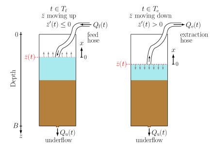
Figure 1. Illustration of an SBR in the two stages that involve flow through the hose: (left) feed and (right) extraction. The boundary $\bar{z}$ moves upward at time $t$ when $\bar{z}^{\prime}(t)<0$ and downward when $\bar{z}^{\prime}(t)>0$, and $T_{\rm f}$ and $T_{\rm e}$ are the feed and extraction time intervals, respectively.

The moving boundary, denoted by $\bar{z}\coloneqq\bar{z}(t)$, where $t\geq 0$ is time, is a known function given by the bulk flows acting on the SBR. The curve $t\mapsto\bar{z}(t)$ defines a spatial change of variables, where in the new variable $\xi$, the top and bottom boundaries are located at $\xi=0$ and $\xi=1$, respectively. The sought vector unknowns, in the variable $\xi$, are the solid phase and liquid substrate components

$$\boldsymbol{C} \coloneqq\boldsymbol{C}(\xi,t)\coloneqq(C^{(1)}(\xi,t),\dots,C^{(k_{\boldsymbol{C}})}(\xi,t))^{\mathrm{T}},\quad\boldsymbol{S}\coloneqq\boldsymbol{S}(\xi,t)\coloneqq(S^{(1)}(\xi,t),\dots,S^{(k_{\boldsymbol{S}})}(\xi,t))^{\mathrm{T}}.$$

The model equations for $0<\xi<1$ are given by

$$\begin{split}\partial_{t}\boldsymbol{C}+\partial_{\xi}\bigl{(}U_{\boldsymbol{C}}(X,\xi,t)\boldsymbol{C}\bigr{)}&=\partial_{\xi}\bigl{(}\gamma(\xi)\beta(t)^{2}\partial_{\xi}\mathcal{D}(X)\bigr{)}\\ &\quad+\beta(t)\bar{z}^{\prime}(t)\boldsymbol{C}+\delta(\xi)\beta(t)q_{\mathrm{f}}(t)\boldsymbol{C}_{\rm f}(t)+\gamma(\xi)\boldsymbol{R}_{\boldsymbol{C}}(\boldsymbol{C},\boldsymbol{S}),\\ \partial_{t}{\boldsymbol{S}}+\partial_{\xi}\bigl{(}U_{\boldsymbol{S}}(X,\xi,t)\boldsymbol{S}\big{)}&=\partial_{\xi}\biggl{(}\frac{\gamma(\xi)\beta(t)^{2}}{\rho_{X}-X}\partial_{\xi}\mathcal{D}(X)\biggr{)}\\ &\quad+\beta(t)\bar{z}^{\prime}(t)\boldsymbol{S}+\delta(\xi)\beta(t)q_{\mathrm{f}}(t)\boldsymbol{S}_{\mathrm{f}}(t)+\gamma(\xi)\boldsymbol{R}_{\boldsymbol{S}}(\boldsymbol{C},\boldsymbol{S}),\end{split}$$ (1.1)

where $U_{\boldsymbol{C}}$ and $U_{\boldsymbol{S}}$ are velocity functions related to the velocities of the solid and liquid phases, respectively, $X\coloneqq(C^{(1)}+\cdots+C^{(k_{\boldsymbol{C}})})/c$ is the total solids concentration, $c$ is a conversion factor, $\beta$ is a given time dependent function, $\rho_{X}$ is the (constant) mass density of solids, and $\mathcal{D}(X)$ is an integrated diffusion coefficient describing compressibility of the sediment. It is assumed that $\mathcal{D}(X)=0$ for $X\leq X_{\mathrm{c}}$, where $X_{\mathrm{c}}>0$ is a critical concentration beyond which the solid particles are assumed to touch each other, so the system (1.1) is of first order wherever $X\leq X_{\mathrm{c}}$, and therefore is strongly degenerate. The second term in the right-hand side of both equations is due to the change of variables in the spatial partial derivative, while the third term contains the feed concentrations $\boldsymbol{C}_{\rm f}$ and $\boldsymbol{S}_{\rm f}$ for the solid and liquid phases, respectively, the feed velocity $q_{\rm f}$, and the Dirac symbol $\delta$. The last terms model the chemical reactions between the components of the solid and liquid phases, where $\boldsymbol{R}_{\boldsymbol{C}}$ and $\boldsymbol{R}_{\boldsymbol{S}}$ are vectors of reaction terms, and $\gamma$ is the characteristic function that equals one inside the tank and zero outside. The system (1.1) is coupled to transport equations modelling the concentrations in the extraction pipe connected at $\xi=0$. (The variables and functions arising in (1.1) are precisely defined in later parts of the paper.)

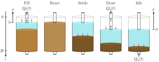
Figure 2. Schematic of the five stages of an SBR. The red arrows show the movement of the boundary or the sediment level during each stage. The black arrows show the direction of the bulk flows $Q_{\rm f}$ (feed), $Q_{\rm e}$ (extraction) and $Q_{\rm u}$ (underflow).

1.2. Related work

Several works posed for SBRs have mostly considered the fill and react stages, where a continuously mixed tank is assumed and the biochemical reactions are modelled by ODEs from some of the established activated sludge models (ASM1, ASM2, ASM2d, or ASM3; in short, AMSx) [25, 31]. We refer to handbooks (e.g., [17, 21, 32] for a broader introduction to the background of wastewater treatment. PDE models for the reactive-settling process have recently been developed [3, 5, 6, 12]. One of the first PDE-based models combining the sedimentation-consolidation process for the batch denitrification in wastewater treatment was presented in [4]. That model consists of five unknowns, two solid components and three substrates, and includes nonlinear terms for the reactions between the solid and liquid components. An extension to the case of continuous sedimentation was introduced in [12], where the model was based on the percentages of the concentrations of the solid and liquid phases. A reliable numerical scheme and simulations of the denitrification process were also included. The present work also utilizes the concept of percentages for sedimentation models, which was introduced in [20]. In [3], the authors presented an alternative reactive settling model which also included non-cylindrical vessels. A numerical scheme based on a method-of-lines formulation was developed and the numerical results are compared with the ones of [12]. Recently, a slightly modified version of that model including extra diffusion terms modelling mixing near the feed inlet has been calibrated to experiments from a pilot plant in [7].

The present SBR model is the one in [5], which is a development of the one in [3] to take into account the moving boundary due to bulk flows of the SBR stages. The settling of particles is allowed in the model in all five stages with the exception of the react one. A conservative and positivity-preserving numerical scheme developed on a fixed mesh grid was introduced in [6]. The scheme of [6] employs careful mass distributions in cells near the moving boundary to ensure the conservation of mass. Simulations of the activated sludge model no. 1 (ASM1) [25] were included in [6] for the case of a cylindrical vessel.

The trajectory of $\bar{z}(t)$ is given, and not part of the solution of the problem, so the governing PDE model (1.1) is a moving boundary problem, but not a free boundary problem. Nevertheless, extensions of the SBR model to a free boundary problem are conceivable. For one scalar PDE related models of filtration have been studied in [14, 8]. Finally, we mention that the formulation and partial analysis of the semi-implicit scheme presented herein is based on anlyses of schemes of that type for degenerate parabolic PDE in [9, 23].

1.3. Outline of the paper

The remainder of this work is organized as follows. In Section 2, we review the SBR model, starting with assumptions on the tank and the one-dimensional model, and explaining the relation between the moving boundary and bulk flows (Section 2.1). The one-dimensional model of the reactive-sedimentation process in the tank is obtained from the balance laws of mass of all the particulate and soluble components. The details of the formulation of the model are outlined in Section 2.2, starting from the solid and liquid components and reactions within the biokinetic reaction model (as an example, we here employ the model ASM1) followed by a summary of the sedimentation-compression model that has also been employed in previous works. The balance laws for the SBR are coupled with transport equations for the pipe. During the react stage with full mixing, the PDEs are replaced by a system of ordinary differential equations (ODEs). While these model ingredients are reviewed from our previous treatment [5, 6], one of the three decisive novelties of the present approach, namely the transformation of the moving boundary model to a fixed computational domain, is formulated in Section 2.3. The second novelty is the reformulation of the governing model in terms of the vector of percentages $\boldsymbol{p}$ (of the solid components, with respect to $X$) done in Section 2.4.

An explicit numerical scheme for the solution of the transformed governing model is introduced in Section 3. This scheme is based on a standard discretization in space and time of the computational domain (Section 3.1). The explicit numerical scheme, presented in Section 3.2, is based on the percentage and fixed-domain formulations of Sections 2.3 and 2.4 and combines upwind discretizations for transport terms, the Engquist-Osher numerical flux [22] for nonlinear flux terms, and a central difference formula for nonlinear degenerating diffusion terms arising in the governing models, combined with appropriate discretizations of the reaction terms. The scheme is complemented by a suitable discretization of the ODEs describing the mixing stage (Section 3.3). It is assumed that the spatial mesh width $\Delta\xi$ and the time step $\tau$ are related by a CFL condition outlined in Section 3.4, and we prove in Section 3.5 that this scheme is montone, with the consequence that an invariant-region principle holds, i.e., solids concentrations are nonnegative and less or equal a maximal one, percentages are nonnegative and sum up to one, and substrate concentrations are nonnegative. The CFL condition for the explicit scheme essentially bounds $\tau/\Delta\xi^{2}$.

A more favorable CFL condition that only bounds $\tau/\Delta\xi$ is associated with a semi-implicit scheme for the governing PDE model, which is the third novelty introduced in Section 4. At each time step, it consists of a nonlinear semi-implicit scheme for the PDE for $X$, which is described in Section 4.1, where we also demonstrate that the nonlinear equations are well posed, i.e., possess a unique solution that depends continuously on data. The solution of the nonlinear equations is achieved by Newton-Raphson method (Section 4.2). Once the scalar function $X$ has been updated, one proceeds to update the vectors $\boldsymbol{p}$ and $\boldsymbol{S}$. This is done by an implicit version of the corresponding $\boldsymbol{p}$- and $\boldsymbol{S}$-schemes of Section 3. This version is, however, linearly implicit and only requires the solution of one linear system per time step, see Section 4.3. In Section 4.4, it is proved that the semi-implicit scheme has the same monotonicity and invariant-region properties as its explicit counterpart (cf. Section 3.5) but does so under the more favorable CFL condition. Numerical examples that illustrate the performance of the numerical schemes of Sections 3 and 4 are presented in Section 5. In particular, it is demonstrated that the semi-implicit scheme indeed leads to the expected gain in efficiency. Finally, conclusions are collected in Section 6.

2. A model of a sequencing batch reactor (SBR)

We here review the assumptions of the general SBR model in [5] and refer to [6] for a full description of the numerical scheme SBR2. That model will then be slightly reformulated, which allows for a semi-implicit numerical scheme to be developed. The sedimentation and compaction properties of the flocculated sludge are namely assumed to depend on the total concentration $X$ and not on the concentrations of the individual components since these are flocculated to larger particles. Each flocculated particle consists of several individual components, which can be described as percentages of the total concentration $X$. For simplicity of writing, we confine here to a constant cross-sectional area $A$, which is the most common case in the applications.

2.1. Assumptions on the tank and the 1D model

The reactor tank is assumed to be a cylindrical vessel with constant horizontal cross-sectional area $A$; see Figure 2. We place a fixed $z$-axis indicating the depth from the top ($z=0$) to the bottom at $z=B$. At the surface of the mixture, located at $z=\bar{z}(t)$, a floating device connected to a pipe allows one to feed the tank at given volumetric feed flow $Q_{\mathrm{f}}(t)$ [m³/s] and feed concentrations $\boldsymbol{C}_{\rm f}(t)$ and $\boldsymbol{S}_{\mathrm{f}}(t)$. The floating device can alternatively extract mixture at a given volume rate $Q_{\mathrm{e}}(t)$ during the draw stage. One cannot fill and draw simultaneously. The extraction pipe is modelled by a half-line and the flow through it by a linear advection PDE. The concentrations in the pipe are denoted by $\boldsymbol{C}_{\mathrm{e}}(t)$ and $\boldsymbol{S}_{\mathrm{e}}(t)$. At the bottom, $z=B$, one can withdraw mixture at a given volume rate $Q_{\mathrm{u}}(t)\geq 0$, and the corresponding output concentrations there are denoted by $\boldsymbol{C}_{\mathrm{u}}(t)$ and $\boldsymbol{S}_{\mathrm{u}}(t)$. We define the bulk velocities

$$q_{\mathrm{u}}(t)\coloneqq Q_{\mathrm{u}}(t)/A,\qquad q_{\mathrm{e}}\coloneqq Q_{\mathrm{e}}(t)/A,\qquad q_{\mathrm{f}}\coloneqq Q_{\mathrm{f}}(t)/A.$$

If $[0,T]$ denotes the total time interval of modelling (and simulation in Section 3), we assume that $T\coloneqq{T}_{\mathrm{e}}\cup{T}_{\mathrm{f}}$, where

$${T}_{\mathrm{e}} \coloneqq\bigl{\{}t\in\mathbb{R}_{+}:Q_{\mathrm{e}}(t)>0,Q_{\mathrm{f}}(t)=0\bigr{\}},\qquad{T}_{\mathrm{f}}\coloneqq\bigl{\{}t\in\mathbb{R}_{+}:Q_{\mathrm{e}}(t)=0,Q_{\mathrm{f}}(t)\geq 0\bigr{\}}$$

(such that ${T}_{\mathrm{e}}\cap{T}_{\mathrm{f}}=\varnothing$). The volume of the mixture at time $t$ is

$$\bar{V}(t)\coloneqq A\big{(}B-\bar{z}(t)\big{)}.$$ (2.1)

The surface location $\bar{z}(t)$ is determined by the given volumetric flows, since by differentiation of (2.1),

$$\bar{z}^{\prime}(t)=-\frac{\bar{V}^{\prime}(t)}{A}=\frac{Q_{\mathrm{u}}(t)-\bar{Q}(t)}{A},\quad\text{where}\quad\bar{Q}(t)\coloneqq\begin{cases}-Q_{\mathrm{e}}(t)<0&\text{if $t\in T_{\mathrm{e}}$},\\ Q_{\mathrm{f}}(t)\geq 0&\text{if $t\in T_{\mathrm{f}}$.}\end{cases}$$

Clearly, $\bar{z}$ is given at any time, so the model under consideration is a moving boundary problem, but not a free boundary problem. That said, we emphasize that because of the volumetric flows, no boundary conditions need to be imposed since the conservation law implies natural output concentrations when reactions and sedimentation are assumed to occur inside the tank only.

2.2. A model of reactive settling with moving boundary

2.2.1. Biochemical reaction model and solid and liquid components

Two constitutive functions describe the sedimentation-compression process of the flocculated particles that consist of several components. These functions are stated in terms of the solids in suspension $X$. This quantity equals the sum of either all or of most of the particulate concentrations; the precise definition of $X$ depends on the specific reaction model. Any biochemical reaction model can be used such as one of the standard ASMx activated sludge models. Within the ASMx models concentrations are usually expressed in terms of more easily measurable units such as chemical oxygen demand (COD) (cf. Table 6 in Appendix A), wherefore conversion factors have to be used to obtain the mass concentrations. We here use the ASM1 model (see Appendix A), in which the particulate concentrations are (in ASM1 units)

$$X_{\mathrm{I}},X_{\mathrm{S}},X_{\mathrm{B,H}},X_{\mathrm{B,A}},X_{\mathrm{P}},X_{\rm ND},$$

and the corresponding definition of the total suspended solids concentration is

$$X\coloneqq c(X_{\mathrm{I}}+X_{\mathrm{S}}+X_{\mathrm{B,H}}+X_{\mathrm{B,A}}+X_{\mathrm{P}}),\quad\text{where $c=0.75\,{\rm g/(g\,COD)}$}.$$

The concentration $X_{\rm ND}$ is not in the definition of $X$, since $X_{\rm ND}$ represents the nitrogen that is already part of $X_{\mathrm{S}}$. To ensure (for mathematical reasons) that the total solids concentration $X$ equals the sum of all particulate components, we replace the variable $X_{\mathrm{S}}$ by $X_{\mathrm{S-ND}}\coloneqq X_{\mathrm{S}}-X_{\mathrm{ND}}$, and define (in ASM1 units)

$$\boldsymbol{C} \coloneqq\big{(}X_{\mathrm{I}},X_{\mathrm{S-ND}},X_{\mathrm{B,H}},X_{\mathrm{B,A}},X_{\mathrm{P}},X_{\rm ND}\big{)}^{\mathrm{T}}\quad\text{(i.e., $k_{\boldsymbol{C}}=6$),}$$

$$\boldsymbol{S} \coloneqq\big{(}S_{\mathrm{I}},S_{\mathrm{S}},S_{\mathrm{O}},S_{\mathrm{NO}},S_{\mathrm{NH}},S_{\mathrm{ND}}\big{)}^{\mathrm{T}}\quad\text{(i.e., $k_{\boldsymbol{S}}=6$).}$$

Moreover, we define

$$X\coloneqq c\big{(}C^{(1)}+\cdots+C^{(k_{\boldsymbol{C}})}\big{)},\qquad p^{(k)}X\coloneqq cC^{(k)},\qquad\boldsymbol{p}X\coloneqq c\boldsymbol{C}.$$ (2.2)

Similar conversion factors as $c$ appear for the soluble concentrations; however, we will divide these factors away directly, since the left-hand sides of the governing equations to be presented are linear in $\boldsymbol{C}$ and $\boldsymbol{S}$ apart from the coefficients, which are nonlinear functions of $X$.

2.2.2. Reaction terms

The nonlinear reaction terms are given by

$$\begin{split}&\boldsymbol{\Lambda}_{\boldsymbol{C}}\boldsymbol{R}_{\boldsymbol{C}}(\boldsymbol{C},\boldsymbol{S}),\quad\text{where}\quad\boldsymbol{R}_{\boldsymbol{C}}(\boldsymbol{C},\boldsymbol{S})\coloneqq\boldsymbol{\sigma}_{\mathrm{\!\boldsymbol{C}}}\boldsymbol{r}(\boldsymbol{C},\boldsymbol{S}),\\ &\boldsymbol{\Lambda}_{\boldsymbol{S}}\boldsymbol{R}_{\boldsymbol{S}}(\boldsymbol{C},\boldsymbol{S}),\quad\text{where}\quad\boldsymbol{R}_{\boldsymbol{S}}(\boldsymbol{C},\boldsymbol{S})\coloneqq\boldsymbol{\sigma}_{\mathrm{\!\boldsymbol{S}}}\boldsymbol{r}(\boldsymbol{C},\boldsymbol{S}),\end{split}$$

which model the increase in (COD) concentration per time unit; see Table 6. Here, $\boldsymbol{\Lambda}_{\boldsymbol{C}}=\operatorname{diag}(c,c,c,c,c,1)$ and $\boldsymbol{\Lambda}_{\boldsymbol{S}}$ are diagonal matrices with conversion factors, $\boldsymbol{\sigma}_{\mathrm{\!\boldsymbol{C}}}$ and $\boldsymbol{\sigma}_{\mathrm{\!\boldsymbol{S}}}$ are constant stoichiometric matrices, and $\boldsymbol{r}(\boldsymbol{C},\boldsymbol{S})\geq\boldsymbol{0}$ is a vector of nonlinear functions modelling the reaction processes; see Appendix A.

We assume that if a solid component is not present, $p^{(k)}=0$, then no more such can vanish, i.e. $\smash{R_{\boldsymbol{C}}^{(k)}(\boldsymbol{C},\boldsymbol{S})|_{p^{(k)}=0}=0}$, where $\smash{R_{\boldsymbol{C}}^{(k)}}$ denotes the $k$-th component of $\boldsymbol{R}_{\boldsymbol{C}}$. Finally, to be able to establish an invariant-region property for the numerical solution, we make some additional technical assumptions. To ensure that the numerical solution for the solids does not exceed the maximal concentration $\hat{X}$, we assume that

$$\text{there exists an $\varepsilon>0$ such that $\boldsymbol{R}_{\boldsymbol{C}}(\boldsymbol{C},\boldsymbol{S})=\boldsymbol{0}$ for all $X\geq\hat{X}-\varepsilon$}.$$ (2.3)

This condition means that when the concentration $X$ is near the maximal one $\hat{X}$, biomass cannot grow any more. To obtain positivity of component $k$ of the concentration vector $\boldsymbol{C}$, we let

$$I_{\boldsymbol{C},k}^{-}:=\big{\{}l\in\mathbb{N}:\sigma_{\boldsymbol{C}}^{(k,l)}<0\big{\}},\qquad I_{\boldsymbol{C},k}^{+}:=\big{\{}l\in\mathbb{N}:\sigma_{\boldsymbol{C}}^{(k,l)}>0\big{\}},$$

denote the sets of indices $l$ that have negative and positive stoichiometric coefficients, respectively, and assume that

$$\text{if $l\in I_{\boldsymbol{C},k}^{-}$, then $r^{(l)}(\boldsymbol{C},\boldsymbol{S})=\bar{r}^{(l)}(\boldsymbol{C},\boldsymbol{S})C^{(k)}$ with $\bar{r}^{(l)}$ bounded}.$$

2.2.3. Bulk velocities and constitutive equations

We define the characteristic function $\chi_{\omega}=1$ if the statement $\omega$ is true, otherwise $\chi_{\omega}=0$. The characteristic function for the tank is thus $\gamma(z,t)=\chi_{\{\bar{z}(t)<z<B\}}(z)$. The bulk velocity of the mixture in the tank and below it in the underflow pipe is defined as $\smash{q(z,t)\coloneqq q_{\mathrm{u}}(t)\chi_{\{z>\bar{z}(t)\}}}$ and the excess velocity due to sedimentation and compression is

$$v\coloneqq v(X,\partial_{z}X,z,t)\coloneqq\gamma(z,t)v_{\mathrm{hs}}(X)\left(1-\dfrac{\rho_{X}\sigma_{\mathrm{e}}^{\prime}(X)}{Xg\Delta\rho}\partial_{z}{X}\right)=\gamma(z,t)\big{(}v_{\mathrm{hs}}(X)-\partial_{z}{D(X)}\big{)}$$

(see [13, 15]), where

$$D(X)\coloneqq\int_{X_{c}}^{X}d(s)\,{\rm d}s,\qquad d(X)\coloneqq v_{\mathrm{hs}}(X)\dfrac{\rho_{X}\sigma_{\mathrm{e}}^{\prime}(X)}{gX\Delta\rho}.$$

Here, $\Delta\rho\coloneqq\rho_{X}-\rho_{L}$ is the density difference of the flocculated particles and the liquid, $g$ is the acceleration of gravity, $v_{\mathrm{hs}}(X)$ is the hindered-settling velocity function, which is assumed to satisfy

$$v_{\mathrm{hs}}(X)\begin{cases}>0&\text{for $X\in[0,\hat{X})$,}\\ =0&\text{for $X\geq\hat{X}$},\end{cases}$$ (2.4)

where $\hat{X}<\rho_{X}$ is a maximum packing concentration (for computational purposes). The second constitutive function is the effective solids stress $\sigma_{\mathrm{e}}(X)$, which satisfies

$$\sigma_{\mathrm{e}}^{\prime}(X)\begin{cases}=0&\text{for $X\leq X_{\mathrm{crit}}$,}\\ >0&\text{for $X>X_{\mathrm{crit}}$,}\end{cases}$$

where $X_{\mathrm{crit}}$ is a critical concentration above which the particles touch each other and form a network that can bear a certain stress.

2.2.4. Balance laws

The balance law of each material component gives the system of PDEs

$$\begin{split}\partial_{t}{\boldsymbol{C}}+\partial_{z}\big{(}\mathcal{V}_{\boldsymbol{C}}(X,\partial_{z}X,z,t)\boldsymbol{C}\big{)}&=\delta\bigl{(}z-\bar{z}(t)\bigr{)}q_{\mathrm{f}}(t)\boldsymbol{C}_{\rm f}+\gamma(z,t)\boldsymbol{R}_{\boldsymbol{C}}(\boldsymbol{C},\boldsymbol{S}),\\ \partial_{t}{\boldsymbol{S}}+\partial_{z}\big{(}\mathcal{V}_{\boldsymbol{S}}(X,\partial_{z}X,z,t)\boldsymbol{S}\big{)}&=\delta\bigl{(}z-\bar{z}(t)\bigr{)}q_{\mathrm{f}}(t)\boldsymbol{S}_{\mathrm{f}}+\gamma(z,t)\boldsymbol{R}_{\boldsymbol{S}}(\boldsymbol{C},\boldsymbol{S}),\end{split}$$ (2.5)

modelling reactive settling for $z\in\mathbb{R}$, where we have divided away the COD factors $c$ etc. in each equation, $\delta(\cdot)$ [m^-1] is the delta symbol, and the total velocities are

$$\begin{split}\mathcal{V}_{\boldsymbol{C}}=\mathcal{V}_{\boldsymbol{C}}(X,\partial_{z}X,z,t)&\coloneqq q(z,t)+\gamma(z,t)\big{(}v_{\mathrm{hs}}(X)-\partial_{z}{D(X)}\big{)},\\ \mathcal{V}_{\boldsymbol{S}}=\mathcal{V}_{\boldsymbol{S}}(X,\partial_{z}X,z,t)&\coloneqq q(z,t)-\gamma(z,t)\frac{(v_{\mathrm{hs}}(X)-\partial_{z}{D(X)})X}{\rho_{X}-X}.\end{split}$$

The pipe of extraction is modelled as a half line $x\geq 0$ (upwards) with $x=0$ coupled at $z=\bar{z}(t)$. Any concentration is assumed to follow the advection equations

$$\partial_{t}\boldsymbol{C}_{\mathrm{pipe}}+q_{\mathrm{e}}(t)\partial_{x}\boldsymbol{C}_{\mathrm{pipe}}=\boldsymbol{0},\quad\partial_{t}\boldsymbol{S}_{\mathrm{pipe}}+q_{\mathrm{e}}(t)\partial_{x}\boldsymbol{S}_{\mathrm{pipe}}=\boldsymbol{0}.$$ (2.6)

The extraction concentrations in the pipe are given by complicated formulas due to the moving boundary; see [5]. With the variable change suggested below, these will be obtained more easily.

2.2.5. Equations during the react stage

During periods of mixing, the system of PDEs (2.5) reduces to the system of ODEs

$$\bar{V}(t)\boldsymbol{C}^{\prime}(t) =\big{(}Q_{\mathrm{u}}(t)-\bar{Q}(t)\big{)}\boldsymbol{C}+Q_{\mathrm{f}}(t)\boldsymbol{C}_{\rm f}(t)+\bar{V}(t)\boldsymbol{R}_{\boldsymbol{C}}(\boldsymbol{C},\boldsymbol{S}),$$

$$\bar{V}(t)\boldsymbol{S}^{\prime}(t) =\big{(}Q_{\mathrm{u}}(t)-\bar{Q}(t)\big{)}\boldsymbol{S}+Q_{\mathrm{f}}(t)\boldsymbol{S}_{\mathrm{f}}(t)+\bar{V}(t)\boldsymbol{R}_{\boldsymbol{S}}(\boldsymbol{C},\boldsymbol{S}),$$

for the homogeneous concentrations in $\bar{z}(t)<z<B$, where all concentrations depend only on time since they are averages in the tank. In the region $z<\bar{z}(t)$ all concentrations are zero, whereas the outlet concentrations are $\boldsymbol{C}_{\rm u}(t)=\boldsymbol{C}(t)$ and $\boldsymbol{C}_{\rm e}(t)=\boldsymbol{C}(t)$ (if $Q_{\mathrm{e}}(t)>0$) (analogously for $\boldsymbol{S}$).

2.3. Model equations on a fixed domain

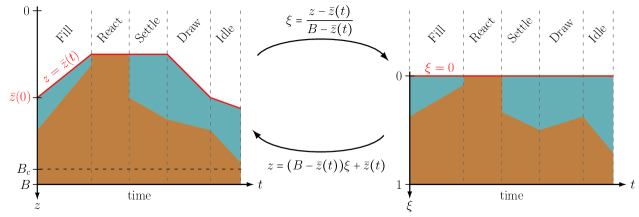
Figure 3. Evolution of a concentration profile varying with respect to time at the five SBR stages in the space variable $z$ (left) and new variable $\xi$ (right). The moving boundary $z=\bar{z}(t)$ (red line) is mapped to the constant line $\xi=0$. The mappings $z=z(\xi,t)$ and $\xi=\xi(z,t)$ are shown in the middle.

To solve the model equations (2.5)–(2.6) without complicated formulas for the outlet concentrations, we transform the time-varying interval $[\bar{z}(t),B]$ to the fixed domain $[0,1]$ for all $t\geq 0$ by introducing the space variable, for all $z\in\mathbb{R}$,

$$\xi=\xi(z,t)\coloneqq\dfrac{z-\bar{z}(t)}{B-\bar{z}(t)}\quad\quad\Leftrightarrow\quad z=(B-\bar{z}(t))\xi+\bar{z}(t).$$ (2.7)

where it is assumed that $B-\bar{z}(t)\geq B_{\mathrm{c}}>0$ for all $t\geq 0$ for some constant $B_{\mathrm{c}}$. We define the unknowns of the model in the new variable $\xi$ by $\tilde{X}(\xi(z,t),t)\coloneqq X(z,t)$ (analogously for the rest of the unknowns and space dependent functions). The partial derivatives are

$$\partial_{t}\xi=-\bar{z}^{\prime}(t)\dfrac{1-\xi}{B-\bar{z}(t)}\eqqcolon\alpha(\xi,t),\qquad\partial_{z}\xi=\dfrac{1}{B-\bar{z}(t)}\eqqcolon\beta(t).$$

Clearly, the sign of $\alpha$ depends uniquely on the slope $\bar{z}^{\prime}$ and therefore on $t$, while $\beta(t)>0$ for all $t>0$. Then the time and space partial derivatives are transformed as

$$\partial_{t}X =\partial_{\xi}\tilde{X}\partial_{t}\xi+\partial_{t}\tilde{X}=\alpha(\xi,t)\partial_{\xi}\tilde{X}+\partial_{t}\tilde{X},\quad\partial_{z}X=\partial_{\xi}\tilde{X}\partial_{z}\xi=\beta(t)\partial_{\xi}\tilde{X}=\partial_{\xi}\bigl{(}\beta(t)\tilde{X}\bigr{)}.$$

It will be convenient to rewrite the term

$$\alpha(\xi,t)\partial_{\xi}\tilde{X}=\partial_{\xi}\bigl{(}\alpha(\xi,t)\tilde{X}\bigr{)}-\partial_{\xi}\alpha(\xi,t)\tilde{X}=\partial_{\xi}\bigl{(}\alpha(\xi,t)\tilde{X}\bigr{)}-\beta(t)\bar{z}^{\prime}(t)\tilde{X}$$

(anticipating the transformation of $\partial_{t}\boldsymbol{C}$ in (2.5) etc.). The characteristic function becomes

$$\gamma(z,t)=\chi_{\{\bar{z}(t)<z<B\}}(z)=\tilde{\chi}_{\{0<\xi<1\}}(\xi)=:\tilde{\gamma}(\xi).$$

The delta symbol in (2.5) is formally transformed via the Heaviside function $H$ as

$$H\bigl{(}z-\bar{z}(t)\bigr{)} =H\big{(}\xi(B-\bar{z}(t))\big{)}=:\tilde{H}(\xi),$$

$$\delta\bigl{(}z-\bar{z}(t)\bigr{)} =H^{\prime}\bigl{(}z-\bar{z}(t)\bigr{)}=\tilde{H}^{\prime}(\xi)=\tilde{H}^{\prime}(\xi)\beta(t)=\tilde{\delta}(\xi)\beta(t).$$

The bulk velocity becomes $q(z,t)=q_{\mathrm{u}}(t)\chi_{\{z>\bar{z}(t)\}}(z)=q_{\mathrm{u}}(t)\tilde{H}(\xi).$ Equations (2.5) can be written in the new variable $\xi$ as the system

$$\begin{split}\partial_{t}{\boldsymbol{C}}+\partial_{\xi}\big{(}\tilde{\mathcal{V}}_{\boldsymbol{C}}(X,\partial_{\xi}X,\xi,t)\boldsymbol{C}\big{)}&=\beta(t)\bar{z}^{\prime}(t)\boldsymbol{C}+\delta(\xi)\beta(t)q_{\mathrm{f}}(t)\boldsymbol{C}_{\rm f}+\gamma(\xi)\boldsymbol{R}_{\boldsymbol{C}}(\boldsymbol{C},\boldsymbol{S})\\ \partial_{t}{\boldsymbol{S}}+\partial_{\xi}\big{(}\tilde{\mathcal{V}}_{\boldsymbol{S}}(X,\partial_{\xi}X,\xi,t)\boldsymbol{S}\big{)}&=\beta(t)\bar{z}^{\prime}(t)\boldsymbol{S}+\delta(\xi)\beta(t)q_{\mathrm{f}}(t)\boldsymbol{S}_{\mathrm{f}}+\gamma(\xi)\boldsymbol{R}_{\boldsymbol{S}}(\boldsymbol{C},\boldsymbol{S}),\end{split}$$ (2.8)

where we directly have removed the tilde above $\boldsymbol{C}$, $\boldsymbol{S}$, $X$, $\gamma$, $H$, and $\delta$, and

$$\tilde{\mathcal{V}}_{\boldsymbol{C}}(X,\partial_{\xi}X,\xi,t) \coloneqq\tilde{q}(\xi,t)+\gamma(\xi)\beta(t)\left(v_{\mathrm{hs}}(X)-\beta(t)\partial_{\xi}D(X)\right),$$

$$\tilde{\mathcal{V}}_{\boldsymbol{S}}(X,\partial_{\xi}X,\xi,t) \coloneqq\tilde{q}(\xi,t)-\gamma(\xi)\beta(t)\frac{f(X)-\beta(t)\partial_{\xi}\mathcal{D}(X)}{\rho_{X}-X},$$

where $\tilde{q}(\xi,t)\coloneqq\alpha(\xi,t)+\beta(t)q_{\mathrm{u}}(t)\tilde{H}(\xi)$ (temporary definition),

$$f(X)\coloneqq v_{\mathrm{hs}}(X)X,$$ (2.9)

and

$$\mathcal{D}(X)\coloneqq\int_{X_{\mathrm{c}}}^{X}a(s)\,\mathrm{d}s,\quad\text{where}\quad a(s)\coloneqq sd(s).$$

Clearly, the governing equations (2.8) can be expressed in the form (1.1) if we define

$$U_{\boldsymbol{C}}(X,\xi,t)\coloneqq\tilde{q}(\xi,t)+\gamma(\xi)\beta(t)v_{\mathrm{hs}}(X),\quad U_{\boldsymbol{S}}(X,\xi,t)\coloneqq\tilde{q}(\xi,t)-\gamma(\xi)\beta(t)\frac{f(X)}{\rho_{X}-X}.$$

Equations (2.8) hold for $\xi\in\mathbb{R}$ when $t\in T_{\mathrm{f}}$ if it is assumed that all concentrations are zero above the surface $\xi<0$. In particular, for the underflow zone $z>B\Leftrightarrow\xi>1$, the equations are

$$\partial_{t}\boldsymbol{C}+\big{(}\alpha(\xi,t)+\beta(t)q_{\mathrm{u}}(t)\big{)}\partial_{\xi}\boldsymbol{C}=\beta(t)\bar{z}^{\prime}(t)\boldsymbol{C},\quad\partial_{t}\boldsymbol{S}+\big{(}\alpha(\xi,t)+\beta(t)q_{\mathrm{u}}(t)\big{)}\partial_{\xi}\boldsymbol{S}=\beta(t)\bar{z}^{\prime}(t)\boldsymbol{S}.$$

To ensure that fluxes have correct units across the surface during extraction ($t\in T_{\mathrm{e}}$), we also need to transform the extraction pipe. The pipe is originally modelled by the upwards-pointing $x$-axis with bulk flow upwards $q_{\mathrm{e}}(t)$ and coupled to the $z$-axis by $-x=z-\bar{z}(t)$. Consequently, the transformation for the extraction pipe is

$$\xi(x,t)\coloneqq\frac{-x}{B-\bar{z}(t)},$$ (2.10)

and $\boldsymbol{C}_{\mathrm{pipe}}(x,t)=\boldsymbol{\tilde{C}}(\xi(x,t),t)$. Then we get

$$\partial_{t}\boldsymbol{C}_{\mathrm{pipe}} =-\partial_{\xi}\boldsymbol{\tilde{C}}\xi\bar{z}^{\prime}(t)\beta(t)+\partial_{t}\boldsymbol{\tilde{C}}=-\bigl{(}\partial_{\xi}(\xi\boldsymbol{\tilde{C}})-\boldsymbol{\tilde{C}}\bigr{)}\bar{z}^{\prime}(t)\beta(t)+\partial_{t}\boldsymbol{\tilde{C}},\quad\partial_{x}\boldsymbol{C}_{\mathrm{pipe}}=-\partial_{\xi}\boldsymbol{\tilde{C}}\beta(t).$$

Equations (2.6) are transformed to (we immediately remove the tildes)

$$\partial_{t}\boldsymbol{C}-\partial_{\xi}\big{(}\beta(t)(\xi\bar{z}^{\prime}(t)+q_{\mathrm{e}}(t))\boldsymbol{C}\big{)} =-\bar{z}^{\prime}(t)\beta(t)\boldsymbol{C},$$

$$\partial_{t}\boldsymbol{S}-\partial_{\xi}\big{(}\beta(t)(\xi\bar{z}^{\prime}(t)+q_{\mathrm{e}}(t))\boldsymbol{S}\big{)} =-\bar{z}^{\prime}(t)\beta(t)\boldsymbol{S},\quad\xi<0.$$

(In comparison to (2.8), there is a minus sign on the right-hand side here.) With the bulk velocity redefined as

$$\tilde{q}(\xi,t)\coloneqq\begin{cases}0&\text{if $\xi<0$ and $q_{\mathrm{e}}(t)=0$},\\ -\beta(t)(\xi\bar{z}^{\prime}(t)+q_{\mathrm{e}}(t))=-\beta(t)(\xi(q_{\mathrm{u}}(t)+q_{\mathrm{e}}(t))+q_{\mathrm{e}}(t))&\text{if $\xi<0$ and $q_{\mathrm{e}}(t)>0$,}\\ \alpha(\xi,t)+\beta(t)q_{\mathrm{u}}(t)=\beta(t)(\xi\bar{z}^{\prime}(t)+q_{\mathrm{u}}(t)-\bar{z}^{\prime}(t))&\text{if $\xi>0$},\end{cases}$$

we thus get the governing equations

$$\begin{split}\partial_{t}{\boldsymbol{C}}+\partial_{\xi}\big{(}\tilde{\mathcal{V}}_{\boldsymbol{C}}(X,\partial_{\xi}X,\xi,t)\boldsymbol{C}\big{)}&=\operatorname*{sgn}(\xi)\bar{z}^{\prime}(t)\beta(t)\boldsymbol{C}+\delta(\xi)\beta(t)q_{\mathrm{f}}(t)\boldsymbol{C}_{\rm f}+\gamma(\xi)\boldsymbol{R}_{\boldsymbol{C}}(\boldsymbol{C},\boldsymbol{S}),\\ \partial_{t}{\boldsymbol{S}}+\partial_{\xi}\big{(}\tilde{\mathcal{V}}_{\boldsymbol{S}}(X,\partial_{\xi}X,\xi,t)\boldsymbol{S}\big{)}&=\operatorname*{sgn}(\xi)\bar{z}^{\prime}(t)\beta(t)\boldsymbol{S}+\delta(\xi)\beta(t)q_{\mathrm{f}}(t)\boldsymbol{S}_{\mathrm{f}}+\gamma(\xi)\boldsymbol{R}_{\boldsymbol{S}}(\boldsymbol{C},\boldsymbol{S}),\end{split}$$ (2.11)

for $\xi\in\mathbb{R}$ and $t\in T_{\mathrm{e}}$. These equations hold for all $t>0$ if we for $t\in T_{\mathrm{f}}$ define all concentrations in $\xi<0$ to be zero; then the system is reduced to (2.8). The salient point of these transformations is that the outlet concentrations are now simply defined by

$$\boldsymbol{C}_{\mathrm{e}}(t) =\boldsymbol{C}(0^{-},t), \boldsymbol{S}_{\mathrm{e}}(t)=\boldsymbol{S}(0^{-},t)\qquad\text{if $t\in T_{\mathrm{e}}$,}$$ (2.12)

$$\boldsymbol{C}_{\mathrm{u}}(t) =\boldsymbol{C}(1^{+},t), \boldsymbol{S}_{\mathrm{u}}(t)=\boldsymbol{S}(1^{+},t)\qquad\text{if $t\in T_{\mathrm{f}}$ and $Q_{\mathrm{u}}(t)>0$.}$$

For other times the outlet concentrations are defined to be zero.

During periods of mixing and $t\in T_{\mathrm{f}}$, the following ODEs for time-dependent concentrations $\boldsymbol{C}(t)$ and $\boldsymbol{S}(t)$ are obtained by averaging Equations (2.8), i.e., integrating over the interval $[0^{-},1)$ when the convective and diffusive terms are zero:

$$\boldsymbol{C}^{\prime}(t) =\beta(t)\bar{z}^{\prime}(t)\boldsymbol{C}+\beta(t)q_{\mathrm{f}}(t)\boldsymbol{C}_{\mathrm{f}}(t)+\boldsymbol{R}_{\boldsymbol{C}}(\boldsymbol{C},\boldsymbol{S}),$$ (2.13)

$$\boldsymbol{S}^{\prime}(t) =\beta(t)\bar{z}^{\prime}(t)\boldsymbol{S}+\beta(t)q_{\mathrm{f}}(t)\boldsymbol{S}_{\mathrm{f}}(t)+\boldsymbol{R}_{\boldsymbol{S}}(\boldsymbol{C},\boldsymbol{S}).$$

The same ODEs are indeed obtained for $t\in T_{\mathrm{e}}$ (then $\boldsymbol{C}_{\mathrm{f}}(t)=\boldsymbol{S}_{\mathrm{f}}(t)=0$).

2.4. Model equations with percentages

The restrictive part of the explicit CFL condition of an explicit scheme is due to the second-order derivative term containing the function $D(X)$, which depends only on the scalar variable $X$. The governing model will be rewritten so that the convective and diffusive terms are clearly seen. Furthermore, to establish boundedness on the total particulate concentration, $0\leq X\leq\hat{X}$, we will rewrite the model in terms of percentages $\boldsymbol{p}$; see (2.2). We define the flux and reaction term of the total solids concentration $X$ by

$$F(\xi,t,X) \coloneqq\tilde{q}(\xi,t)X+\gamma(\xi)\beta(t)f(X),\qquad{R}(\boldsymbol{C},\boldsymbol{S})\coloneqq c\sum_{k=1}^{k_{\boldsymbol{C}}}R_{\boldsymbol{C}}^{(k)}(\boldsymbol{C},\boldsymbol{S}).$$

Then we can write

$$\tilde{\mathcal{V}}_{\boldsymbol{C}}X =F(\xi,t,X)-\gamma(\xi)\beta(t)^{2}\partial_{\xi}\mathcal{D}(X),\quad\tilde{\mathcal{V}}_{\boldsymbol{S}}=\frac{\tilde{q}(\xi,t)\rho_{X}-F(\xi,t,X)+\gamma(\xi)\beta(t)^{2}\partial_{\xi}\mathcal{D}(X)}{\rho_{X}-X}.$$

By first multiplying the first equation of (2.11) by $c$ and adding the vector components corresponding to (2.2), one obtains the scalar equation

$$\begin{split}\partial_{t}{X}+\partial_{\xi}F(\xi,t,X)&=\partial_{\xi}\big{(}\gamma(\xi)\beta(t)^{2}\partial_{\xi}\mathcal{D}(X)\big{)}\\ &\quad+\beta(t)\operatorname*{sgn}(\xi)\bar{z}^{\prime}(t)X+\beta(t)\delta(\xi)q_{\mathrm{f}}(t)X_{\mathrm{f}}+\gamma(\xi){R}(\boldsymbol{p}X/c,\boldsymbol{S})\end{split}$$ (2.14)

for $X$. The concentrations $\boldsymbol{C}=\boldsymbol{p}X/c$ and $\boldsymbol{S}$ are given by the system (2.11), which we now can rewrite with the unknowns $X$, $\boldsymbol{p}$ and $\boldsymbol{S}$:

$$\partial_{t}{(\boldsymbol{p}X)}+\partial_{\xi}(F(\xi,t,X)\boldsymbol{p}) =\partial_{\xi}\big{(}\boldsymbol{p}\gamma(\xi)\beta(t)^{2}\partial_{\xi}\mathcal{D}(X)\big{)}+\beta(t)\operatorname*{sgn}(\xi)\bar{z}^{\prime}(t)\boldsymbol{p}X$$

$$\qquad+\beta(t)\delta(\xi)q_{\mathrm{f}}(t)\boldsymbol{p}_{\mathrm{f}}X_{\mathrm{f}}+\gamma(\xi)c\boldsymbol{R}_{\boldsymbol{C}}(\boldsymbol{p}X/c,\boldsymbol{S}),$$ (2.15)

$$\partial_{t}{\boldsymbol{S}}+\partial_{\xi}\big{(}\tilde{\mathcal{V}}_{\boldsymbol{S}}\boldsymbol{S}\big{)} =\beta(t)\operatorname*{sgn}(\xi)\bar{z}^{\prime}(t)\boldsymbol{S}+\beta(t)\delta(\xi)q_{\mathrm{f}}(t)\boldsymbol{S}_{\mathrm{f}}+\gamma(\xi)\boldsymbol{R}_{\boldsymbol{S}}(\boldsymbol{p}X/c,\boldsymbol{S}).$$ (2.16)

Not all equations in (2.15) need to be solved; one may solve only the first $k_{\mathrm{\boldsymbol{C}}}-1$ ones and set $p^{(k_{\boldsymbol{C}})}=1-(p^{(1)}+\cdots+p^{(k_{\boldsymbol{C}}-1)})$. The output concentrations for $\boldsymbol{p}$ and $X$ are defined as in (2.12).

The mixing ODEs (2.13) are converted analogously:

$$X^{\prime}(t) =\beta(t)\bar{z}^{\prime}(t)X+\beta(t)q_{\mathrm{f}}(t)X_{\mathrm{f}}(t)+{R}(\boldsymbol{p}X/c,\boldsymbol{S}),$$ (2.17)

$$(\boldsymbol{p}X)^{\prime}(t) =\beta(t)\bar{z}^{\prime}(t)\boldsymbol{p}X+\beta(t)q_{\mathrm{f}}(t)\boldsymbol{p}_{\mathrm{f}}(t)X_{\mathrm{f}}(t)+c\boldsymbol{R}_{\boldsymbol{C}}(\boldsymbol{p}X/c,\boldsymbol{S}),$$

$$\boldsymbol{S}^{\prime}(t) =\beta(t)\bar{z}^{\prime}(t)\boldsymbol{S}+\beta(t)q_{\mathrm{f}}(t)\boldsymbol{S}_{\mathrm{f}}(t)+\boldsymbol{R}_{\boldsymbol{S}}(\boldsymbol{p}X/c,\boldsymbol{S}).$$

3. Explicit numerical scheme

3.1. Discretization in space and time

To discretize the PDE system (2.14)–(2.16), we define $\Delta\xi\coloneqq 1/(N+1/2)$ for an integer $N$, $\xi_{j}\coloneqq j\Delta\xi$, and let cell $j$ be the interval $I_{j}\coloneqq[\xi_{j-1/2},\xi_{j+1/2}]$; see Figure 4.

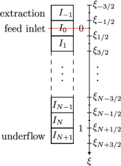
Figure 4. Schematic of the division of the computational domain into cells.

Thus, the feed inlet is located in the middle of $I_{0}$, which makes the numerical fluxes at the cell boundaries easy to define. The bottom of the tank is located at $\xi=\xi_{N+1/2}=(N+1/2)\Delta\xi=1$. Given a total simulation time $T$ and the total number of discrete time points $N_{T}$, we define the time step $\tau\coloneqq T/N_{T}$, which is supposed to satisfy a suitable CFL condition, and the discrete time points $t^{n}$, $n=0,1,\dots,N_{T}$. The total particulate concentration is denoted by $\smash{X_{j}^{n}\approx X(\xi_{j},t^{n})}$, and analogous notation is used for other concentrations. The underflow concentration is captured by an additional cell $j=N+1$ below the tank. The extraction concentrations can be obtained in an analogous way in an additional cell $I_{-1}$. For both the explicit and implicit schemes the outlet concentrations are defined by $\smash{\boldsymbol{p}_{\mathrm{e}}=\boldsymbol{p}_{-1}^{n}}$ and $\smash{\boldsymbol{p}_{\mathrm{u}}=\boldsymbol{p}_{N+1}^{n}}$, and similarly for $X$ and $\boldsymbol{S}$.

3.2. Explicit scheme

For ease of notation, we introduce $a^{+}=\max\{0,a\}$, $a^{-}=\min\{0,a\}$, the upwind and the divergence operators by

$$\operatorname*{Upw}(a;b,c) \coloneqq\max\{a,0\}b+\min\{a,0\}c=a^{+}b+a^{-}c,\qquad\mbox{for }a,b,c\in\mathbb{R},$$

$$[\Delta\boldsymbol{\Phi}]_{j}^{n} \coloneqq\boldsymbol{\Phi}_{j+1/2}^{n}-\boldsymbol{\Phi}_{j-1/2}^{n}.$$

We define the Kronecker delta and the characteristic function for the mixture in the tank by

$$\delta_{j,0}\coloneqq\int_{I_{j}}\delta(\xi)\,\mathrm{d}\xi=\begin{cases}1&\text{if $j=0$},\\ 0&\text{if $j\neq 0$},\end{cases}\qquad\gamma_{j}\coloneqq\begin{cases}\gamma(\xi_{j})&\text{if $j\neq 0$,}\\ \frac{1}{2}&\text{if $j=0$.}\end{cases}$$

The term $\operatorname*{sgn}(\xi)\beta(t)\bar{z}^{\prime}(t)X(\xi,t)$ in (2.14) is approximated by the average

$$\frac{1}{\Delta\xi}\int_{\xi_{-1/2}}^{\xi_{1/2}}\operatorname*{sgn}(\xi)\beta^{n}(\bar{z}^{\prime})^{n}X(\xi,)\,\mathrm{d}\xi=\begin{cases}0&\text{if $q_{\mathrm{e}}^{n}>0$},\\ \frac{1}{2}\beta^{n}(\bar{z}^{\prime})^{n}X_{0}^{n}=\frac{1}{2}\beta^{n}(q_{\mathrm{u}}^{n}-q_{\mathrm{f}}^{n})X_{0}^{n}&\text{if $q_{\mathrm{e}}^{n}=0$},\end{cases}$$

for $j=0$, where we recall that $X(\xi,t)=0$ for $\xi<0$ if $q_{\mathrm{e}}(t)=0$, and analogously for $\boldsymbol{S}$ instead of $X$. For the numerical update formulas, we define

$$\kappa^{n}_{j}\coloneqq\begin{cases}1-\tau\beta^{n}(\bar{z}^{\prime})^{n}=1-\tau\beta^{n}(q_{\mathrm{u}}^{n}+q_{\mathrm{e}}^{n})&\text{if $j<0$ and $q_{\mathrm{e}}^{n}>0$},\\ 1&\text{if $j<0$ and $q_{\mathrm{e}}^{n}=0$ or $j=0$ and $q_{\mathrm{e}}^{n}>0$},\\ 1-\frac{\tau}{2}\beta^{n}(q_{\mathrm{u}}^{n}-q_{\mathrm{f}}^{n})&\text{if $j=0$ and $q_{\mathrm{e}}^{n}=0$,}\\ 1+\tau\beta^{n}(\bar{z}^{\prime})^{n}&\text{if $j>0$,}\end{cases}$$ (3.1)

Finally, we define

$$\tilde{q}_{j+1/2}^{n}\coloneqq\tilde{q}(\xi_{j+1/2},t^{n})=\begin{cases}0&\text{if $j=-2,-1$ and $q_{\mathrm{e}}^{n}=0$,}\\ -\beta^{n}(\xi_{j+1/2}(q_{\mathrm{u}}^{n}+q_{\mathrm{e}}^{n})+q_{\mathrm{e}}^{n})&\text{if $j=-2,-1$ and $q_{\mathrm{e}}^{n}>0$,}\\ \alpha_{j+1/2}^{n}+\beta^{n}q_{\mathrm{u}}^{n}&\text{if $j=0,\ldots,N+1$}.\end{cases}$$

An explicit approximation of the system (2.14)–(2.16) is now obtained by following ideas from [12, 3]. We assume that the function $f$ defined by (2.9) has a unique maximum at $X^{*}\in(0,\hat{X})$. The Engquist-Osher numerical flux [22]

$$\mathcal{E}_{j+1/2}^{n} \coloneqq\gamma_{j+1/2}\biggl{(}f(0)+\int_{0}^{X_{j}^{n}}\max\bigl{\{}0,f^{\prime}(s)\bigr{\}}\,\mathrm{d}s+\int_{0}^{X_{j+1}^{n}}\min\bigl{\{}0,f^{\prime}(s)\bigr{\}}\,\mathrm{d}s\biggr{)}$$ (3.2)

is used, which for a unimodal flux function $f$ is

$$\mathcal{E}_{j+1/2}^{n}\bigl{(}X_{j}^{n},X_{j+1}^{n}\bigr{)}=\gamma_{j+1/2}\begin{cases}f(X_{j}^{n})&\text{if $X_{j}^{n},X_{j+1}^{n}\leq X^{*}$,}\\ f(X^{*})&\text{if $X_{j+1}^{n}\leq X^{*}<X_{j}^{n}$,}\\ -f(X^{*})+f(X_{j}^{n})+f(X_{j+1}^{n})&\text{if $X_{j}^{n}\leq X^{*}<X_{j+1}^{n}$,}\\ f(X_{j+1}^{n})&\text{if $X^{*}<X_{j}^{n},X_{j+1}^{n}$.}\end{cases}$$

The diffusive term and the other fluxes are discretized by

$$\mathcal{J}_{j+1/2}^{n} \coloneqq\gamma_{j+1/2}\dfrac{(\beta^{n})^{2}}{\Delta\xi}\big{(}\mathcal{D}(X^{n}_{j+1})-\mathcal{D}(X^{n}_{j})\big{)},\quad j=-2,\dots,N+1,$$ (3.3)

$$\mathcal{B}_{j+1/2}^{n} \coloneqq{\rm Upw}(\tilde{q}_{j+1/2}^{n};X^{n}_{j},X^{n}_{j+1}),$$ (3.4)

$$\mathcal{F}_{j+1/2}^{n} \coloneqq\mathcal{B}_{j+1/2}^{n}+\beta^{n}\mathcal{E}_{j+1/2}^{n}$$

$$=\begin{cases}0&\text{if $j=-2,-1$ and $q_{\mathrm{e}}^{n}=0$,}\\ -\beta^{n}\big{(}\xi_{j+1/2}(q_{\mathrm{u}}^{n}+q_{\mathrm{e}}^{n})+q_{\mathrm{e}}^{n}\big{)}X^{n}_{j+1}&\text{if $j=-2,-1$ and $q_{\mathrm{e}}^{n}>0$,}\\ {\rm Upw}(\alpha_{j+1/2}^{n}+\beta^{n}q_{\mathrm{u}}^{n};X^{n}_{j},X^{n}_{j+1})+\beta^{n}\mathcal{E}_{j+1/2}^{n}&\text{if $j=0,\dots,N-1$,}\\ (\alpha_{j+1/2}^{n}+\beta^{n}q_{\mathrm{u}}^{n})X^{n}_{j}&\text{if $j=N,N+1$,}\end{cases}$$ (3.5)

$$\Phi_{j+1/2}^{n} \coloneqq\mathcal{F}_{j+1/2}^{n}-\mathcal{J}_{j+1/2}^{n}.$$ (3.6)

We have $\alpha_{N+1/2}=0$, and when $q_{\mathrm{e}}>0$, we assume that $\Delta\xi$ is sufficiently small, so that all fluxes at the top $\xi=\xi_{-1/2}$ and bottom $\xi_{N+1/2}$ are directed out of the tank, which means that no boundary values are needed. The numerical fluxes are then defined, for $j=-2,\dots,N+1$, by

$$\boldsymbol{\Phi}_{\boldsymbol{p},j+1/2}^{n} \coloneqq\operatorname*{Upw}(\Phi_{j+1/2}^{n};\boldsymbol{p}_{j}^{n},\boldsymbol{p}_{j+1}^{n}),$$ (3.7)

$$\boldsymbol{\Phi}_{\boldsymbol{S},j+1/2}^{n} \coloneqq\operatorname*{Upw}\biggl{(}\rho_{X}\tilde{q}_{j+1/2}^{n}-\Phi_{j+1/2}^{n};\frac{\boldsymbol{S}_{j}^{n}}{\rho_{X}-X_{j}^{n}},\frac{\boldsymbol{S}_{j+1}^{n}}{\rho_{X}-X_{j+1}^{n}}\biggr{)}.$$

With an Euler time step, $\lambda\coloneqq\tau/\Delta\xi$, and $\mu\coloneqq\tau/\Delta\xi^{2}$, we can formulate the explicit scheme as follows. For the boundary layers $j=-1$ and $j=N+1$, we set

$$X_{-1}^{n+1}=0,\quad\boldsymbol{p}_{-1}^{n+1}=\boldsymbol{0},\quad\boldsymbol{S}_{-1}^{n+1}=\boldsymbol{0}\quad q_{\mathrm{e}}^{n}=0$$ if , (3.8)

$$X_{N+1}^{n+1}=0,\quad\boldsymbol{p}_{N+1}^{n+1}=\boldsymbol{0},\quad\boldsymbol{S}_{N+1}^{n+1}=\boldsymbol{0}\quad q_{\mathrm{u}}^{n}=0$$ if . (3.9)

Otherwise, we have for $j=-1,\dots,N+1$,

$$X^{n+1}_{j} =\kappa_{j}^{n}X^{n}_{j}-\lambda[\Delta\mathcal{F}]_{j}^{n}+\lambda[\Delta\mathcal{J}]_{j}^{n}+\lambda\delta_{j,0}\beta^{n}q_{\rm f}^{n}X_{\rm f}^{n}+\tau\gamma_{j}{R}(\boldsymbol{p}_{j}^{n}X^{n}_{j}/c,\boldsymbol{S}_{j}^{n}),$$ (3.10)

$$\boldsymbol{p}^{n+1}_{j}X^{n+1}_{j} =\kappa_{j}^{n}\boldsymbol{p}^{n}_{j}X^{n}_{j}-\lambda[\Delta\boldsymbol{\Phi}_{\boldsymbol{p}}]_{j}^{n}+\lambda\delta_{j,0}\beta^{n}q_{\rm f}^{n}\boldsymbol{p}_{\rm f}^{n}X_{\rm f}^{n}+\tau\gamma_{j}c\boldsymbol{R}_{\boldsymbol{C}}(\boldsymbol{p}_{j}^{n}X^{n}_{j}/c,\boldsymbol{S}_{j}^{n}),$$ (3.11)

$$\boldsymbol{S}^{n+1}_{j} =\kappa_{j}^{n}\boldsymbol{S}^{n}_{j}-\lambda[\Delta\boldsymbol{\Phi}_{\boldsymbol{S}}]_{j}^{n}+\lambda\delta_{j,0}\beta^{n}q_{\rm f}^{n}\boldsymbol{S}_{\rm f}^{n}+\tau\gamma_{j}\boldsymbol{R}_{\boldsymbol{S}}(\boldsymbol{p}_{j}^{n}X^{n}_{j}/c,\boldsymbol{S}_{j}^{n}).$$ (3.12)

Scheme (3.10) is solved first, then the others. If $\smash{X^{n+1}_{j}=}0$, then the value of $\smash{\boldsymbol{p}_{j}^{n+1}}$ is irrelevant, and can be set to $\smash{\boldsymbol{p}_{j}^{n+1}\coloneqq\boldsymbol{p}_{j}^{n}}$. For the cells outside the tank, the scheme for $X$ is reduced to the following. If $q_{\mathrm{e}}^{n}=0$, then (3.8) handles $j=-1$; otherwise, we define $q_{\mathrm{out}}^{n}:=q_{\mathrm{u}}^{n}+q_{\mathrm{e}}^{n}$ and utilize

$$X^{n+1}_{-1} =\bigl{(}1-\tau\beta^{n}q_{\mathrm{out}}^{n}\bigr{)}X^{n}_{-1}+\lambda\beta^{n}\bigl{(}(\xi_{-1/2}q_{\mathrm{out}}^{n}+q_{\mathrm{e}}^{n})X^{n}_{0}-(\xi_{-3/2}q_{\mathrm{out}}^{n}+q_{\mathrm{e}}^{n})X^{n}_{-1}\bigr{)},$$ (3.13)

On the other hand, if $q_{\mathrm{u}}^{n}=0$, then (3.9) is in effect for $j=N+1$; otherwise,

$$X^{n+1}_{N+1} =(1+\tau\beta^{n}q_{\mathrm{out}}^{n})X^{n}_{N+1}-\lambda\bigl{(}(\alpha^{n}_{N+3/2}+\beta^{n}q_{\mathrm{u}}^{n})X^{n}_{N+1}-\beta^{n}q_{\mathrm{u}}^{n}X^{n}_{N}\bigr{)}.$$ (3.14)

Similar update formulas hold for $\boldsymbol{p}$ and $\boldsymbol{S}$. The resulting approximate concentrations are transformed back to the original $z$- and $x$-coordinates via (2.7) and (2.10), respectively.

3.3. Numerics during mixing

Suppose a (PDE or numerical) solution $X(\xi,T_{0})$ (or $\smash{p^{(k)}(\xi,T_{0})}$ or $\smash{S^{(k)}(\xi,T_{0}))}$ is known at $t=T_{0}=t_{n_{0}}$ when a period of complete mixing starts. The initial concentrations for the ODEs (2.17) are defined as the averages (analogously for $p^{(k)}$ and $S^{(k)}$)

$$X(T_{0})\coloneqq\int_{0}^{1}X(\xi,T_{0})\,\mathrm{d}\xi\approx\Delta\xi\biggl{(}\frac{X_{0}^{n_{0}}}{2}+{X}_{1}^{n_{0}}+\dots+{X}_{N}^{n_{0}}\biggr{)}.$$

The ODE system (2.17) can then approximately be integrated in time with an Euler step. If an ODE mixing period ends at $t=t^{{n}}$ with the values ${X}(t^{n})$, and the PDE model is to be simulated thereafter, then the value of each component $k$ is allocated to all cells in the tank; ${X}_{j}^{{n}}\coloneqq{X}(t^{n})$, $j=0,\ldots,N$.

3.4. CFL condition

We denote the solution variables by $\mathbfcal{U}\coloneqq(X,\boldsymbol{p}^{\mathrm{T}},\boldsymbol{S}^{\mathrm{T}})^{\mathrm{T}}$ and define the constants

$$\|f\|\coloneqq\max\limits_{0\leq X\leq\hat{X}}|f(X)|, M_{R}\coloneqq\frac{1}{c}\sup_{\boldsymbol{\mathcal{U}}\in\Omega\atop 1\leq k\leq k_{\boldsymbol{C}}}\left|\frac{\partial R}{\partial C^{(k)}}\right|,$$

$$M_{q1}\coloneqq\max_{0\leq t\leq T}\{q_{\mathrm{u}}(t)+q_{\mathrm{e}}(t),q_{\mathrm{f}}(t)\}, M_{q2}\coloneqq\max_{0\leq t\leq T}\big{(}\max\{q_{\mathrm{f}}(t),q_{\mathrm{e}}(t)\}+2q_{\mathrm{u}}(t)\big{)}$$

$$\zeta\coloneqq\frac{1}{B-B_{\mathrm{c}}}, C_{1}\coloneqq\zeta(M_{q2}+\|f^{\prime}\|),$$

$$C_{2}\coloneqq\zeta^{2}\|a\|, M_{\boldsymbol{\xi}}:=\sup_{\boldsymbol{\mathcal{U}}\in\Omega,\atop 1\leq k\leq k_{\boldsymbol{\xi}}}\sum_{l\in I_{\boldsymbol{\xi},k}^{-}}|\sigma_{\boldsymbol{\xi}}^{(k,l)}|\bar{r}_{\boldsymbol{\xi}}^{(l)}(\boldsymbol{C},\boldsymbol{S}),\quad\boldsymbol{\xi}\in\{\boldsymbol{C},\boldsymbol{S}\}.$$

The time step $\tau$ and the spatial mesh width $\Delta\xi$ should satisfy the CFL condition

$$\begin{split}\tau\biggl{(}&\zeta M_{q1}+\max\{M_{R},M_{\boldsymbol{C}},M_{\boldsymbol{S}}\}+\frac{2}{\Delta\xi}\max\biggl{\{}C_{1}+\frac{C_{2}}{\Delta\xi},\frac{1}{\rho_{X}-\hat{X}}\biggl{(}\zeta\rho_{X}+C_{1}\hat{X}+\frac{C_{2}\hat{X}}{\Delta\xi}\biggr{)}\biggr{\}}\biggr{)}\leq 1.\end{split}$$ (CFL)

3.5. Monotonicity and invariant region property

In what follows, we demonstrate that the solution variables $\mathbfcal{U}=(X,\boldsymbol{p}^{\mathrm{T}},\boldsymbol{S}^{\mathrm{T}})^{\mathrm{T}}$ produced by the explicit numerical scheme stays in the set

$$\Omega:=\big{\{}\boldsymbol{\mathcal{U}}\in\mathbb{R}^{1+k_{\boldsymbol{C}}+k_{\boldsymbol{S}}}:0\leq X\leq\hat{X},\ \boldsymbol{p}\geq 0,\ p^{(1)}+\cdots+p^{(k_{\boldsymbol{C}})}=1,\ \boldsymbol{S}\geq 0\big{\}}$$

provided that this property holds for the initial values. Our proofs rely on the following lemma, which follows directly from the definition (3.2).

Lemma 3.1.

Assume that $0\leq X_{j}\leq\hat{X}$ for all $j$. Then the Engquist-Osher flux $\mathcal{E}_{j+1/2}={\mathcal{E}}_{j+1/2}(X_{j},X_{j+1})$ applied on the unimodal function $0\leq f\in C^{1}$ satisfies

$$-\|f^{\prime}\|\leq\frac{\partial\mathcal{E}_{j+1/2}}{\partial X_{j+1}}\leq 0\leq\frac{\partial\mathcal{E}_{j+1/2}}{\partial X_{j}}\leq\|f^{\prime}\|,\quad\left|\frac{\partial[\Delta\mathcal{E}]_{j}}{\partial X_{j}}\right|\leq\|f^{\prime}\|,\quad\frac{\mathcal{E}_{j+1/2}}{X_{j}}\leq\|f^{\prime}\|,\quad\frac{\mathcal{E}_{j+1/2}}{X_{j+1}}\leq\|f^{\prime}\|.$$

Lemma 3.2.

If $\boldsymbol{\mathcal{U}}_{j}^{n}\in\Omega$ for all $j$, then the following estimates hold for $j=-1,\ldots,N+1$:

$$\kappa^{n}_{j}\geq 1-\zeta\tau M_{q1},$$ (3.15)

$$|\tilde{q}_{j+1/2}^{n}|\leq\zeta(\max\{q_{\mathrm{f}}^{n},q_{\mathrm{e}}^{n}\}+2q_{\mathrm{u}}^{n})\leq\zeta M_{q2},$$ (3.16)

$$\frac{\partial[\Delta\mathcal{B}]_{j}^{n}}{\partial X_{k}^{n}}\begin{cases}=-\tilde{q}_{j-1/2}^{n,+}\leq 0&\text{\em if $k=j-1$,}\\ \leq\zeta M_{q2},&\text{\em if $k=j$,}\\ =\tilde{q}_{j+1/2}^{n,-}\leq 0,&\text{\em if $k=j+1$,}\\ =0&\text{\em otherwise},\end{cases}$$ (3.17)

$$\left|\frac{\partial}{\partial X_{k}}R(\boldsymbol{p}_{j}^{n}X_{j}^{n}/c,\boldsymbol{S}_{j}^{n})\right|\begin{cases}\leq{M_{R}}&\text{\em if $k=j$,}\\ =0&\text{\em if $k\neq j$,}\end{cases}$$ (3.18)

$$\max\big{\{}\Phi_{j+1/2}^{n,+},-\Phi_{j-1/2}^{n,-}\big{\}}\leq\left(\zeta({M_{q2}+\|f^{\prime}\|})+\frac{\zeta^{2}\|a\|}{\Delta\xi}\right)X_{j}^{n}$$ (3.19)

Proof.

By the definition of the transformation of variables,

$$-q_{\mathrm{f}}(t) \leq\bar{z}^{\prime}(t)\leq q_{\mathrm{u}}(t)+q_{\mathrm{e}}(t),\qquad-\zeta{(q_{\mathrm{u}}(t)+q_{\mathrm{e}}(t))}\leq\alpha(\xi,t)\leq{\zeta q_{\mathrm{f}}(t)},\qquad 0<\beta(t)\leq\zeta.$$

These inclusions directly imply (3.15) since

$$\kappa^{n}_{j} \geq 1-{\tau\zeta\max\{q_{\mathrm{u}}^{n}+q_{\mathrm{e}}^{n},q_{\mathrm{f}}^{n}\}}\geq 1-{\tau\zeta M_{q1}}.$$

To prove (3.16) we observe that when $q_{\mathrm{e}}^{n}=0$, then $\tilde{q}_{-1/2}^{n}=\tilde{q}_{-3/2}^{n}=0$, and when $q_{\mathrm{e}}^{n}>0$ and $j=-1,-2$,

$$\tilde{q}_{j+1/2}^{n}=-\beta^{n}\big{(}\xi_{j+1/2}(q_{\mathrm{u}}^{n}+q_{\mathrm{e}}^{n})+q_{\mathrm{e}}^{n}\big{)}\geq-{\zeta q_{\mathrm{e}}^{n}}.$$ (3.20)

For $j=0,\ldots,N$, (we recall that if $q_{\mathrm{f}}^{n}>0$, then $q_{\mathrm{e}}^{n}=0$ and vice versa)

$$\tilde{q}_{j+1/2}^{n}=\alpha_{j+1/2}^{n}+\beta^{n}q_{\mathrm{u}}^{n}=\beta^{n}\left({-(\bar{z}^{\prime})^{n}(1-\xi_{j+1/2})+q_{\mathrm{u}}^{n}}\right)\begin{cases}\leq\zeta(q_{\mathrm{f}}^{n}+q_{\mathrm{u}}^{n})&\text{if $q_{\mathrm{e}}^{n}=0$,}\\ \geq-\zeta(q_{\mathrm{u}}^{n}+q_{\mathrm{e}}^{n})&\text{if $q_{\mathrm{e}}^{n}>0$,}\end{cases}$$ (3.21)

and for $j=N+1$,

$$\tilde{q}_{N+3/2}^{n}=\frac{(\bar{z}^{\prime})^{n}\Delta\xi+q_{\mathrm{u}}^{n}}{B-\bar{z}^{n}}\leq\zeta({q_{\mathrm{out}}^{n}\Delta\xi+q_{\mathrm{u}}^{n}})\leq\zeta((1+\Delta\xi)q_{\mathrm{u}}^{n}+q_{\mathrm{e}}^{n}).$$ (3.22)

From (3.20) to (3.22) we now deduce (3.16). Next, computing the difference of the flux

$$\mathcal{B}_{j+1/2}^{n}=\tilde{q}_{j+1/2}^{n,+}X_{j}^{n}+\tilde{q}_{j+1/2}^{n,-}X_{j+1}^{n}$$

and differentiating this expression with respect to $X_{k}^{n}$ we obtain

$$\frac{\partial[\Delta\mathcal{B}]_{j}^{n}}{\partial X_{k}^{n}} =\frac{\partial}{\partial X_{k}^{n}}\bigl{(}\tilde{q}_{j+1/2}^{n,+}X_{j}^{n}+\tilde{q}_{j+1/2}^{n,-}X_{j+1}^{n}-\tilde{q}_{j-1/2}^{n,+}X_{j-1}^{n}-\tilde{q}_{j-1/2}^{n,-}X_{j}^{n}\bigr{)}$$

$$=\begin{cases}-\tilde{q}_{j-1/2}^{n,+}\leq 0&\text{if $k=j-1$,}\\ \tilde{q}_{j+1/2}^{n,+}-\tilde{q}_{j-1/2}^{n,-}\leq\zeta\big{(}{(1+\Delta\xi)q_{\mathrm{u}}^{n}+\max\{q_{\mathrm{e}}^{n},q_{\mathrm{f}}^{n}\}}\big{)}\leq\zeta{M_{q2}}&\text{if $k=j$,}\\ \tilde{q}_{j+1/2}^{n,-}\leq 0&\text{if $k=j+1$,}\\ 0&\text{otherwise}.\end{cases}$$

This proves (3.17). For the reaction term, the cases $k\neq j$ are trivial. Assuming that $k=j$ and differentiating we obtain

$$\left|\frac{\partial}{\partial X_{j}}R(\boldsymbol{p}_{j}^{n}X_{j}^{n}/c,\boldsymbol{S}_{j}^{n})\right|=\frac{1}{c}\left|(\boldsymbol{p}_{j}^{n})^{\mathrm{T}}\nabla_{\!\boldsymbol{C}}R\right|\leq\frac{1}{c}\sum_{i=1}^{k_{\boldsymbol{C}}}p_{j}^{(i),n}\biggl{|}\frac{\partial R}{\partial C_{j}^{(i),n}}\biggr{|}=M_{R}\sum_{i=1}^{k_{\boldsymbol{C}}}p_{j}^{(i),n}=M_{R},$$

which implies (3.18). Finally, (3.19) follows from

$$\Phi_{j+1/2}^{n,+} =\big{(}\mathcal{B}_{j+1/2}^{n}+\beta^{n}\mathcal{E}_{j+1/2}^{n}-\mathcal{J}_{j+1/2}^{n}\big{)}^{+}\leq\tilde{q}_{j+1/2}^{n,+}X_{j}^{n}+\zeta{\|f^{\prime}\|}X_{j}^{n}+\gamma_{j+1/2}\frac{(\beta^{n})^{2}}{\Delta\xi}\mathcal{D}(X_{j}^{n})$$

$$\leq\biggl{(}\zeta({M_{q2}+\|f^{\prime}\|})+\zeta^{2}\frac{\|a\|}{\Delta\xi}\biggr{)}X_{j}^{n},$$

$$-\Phi_{j-1/2}^{n,-} =-\big{(}\mathcal{B}_{j-1/2}^{n}+\beta^{n}\mathcal{E}_{j-1/2}^{n}-\mathcal{J}_{j-1/2}^{n}\big{)}^{-}\leq\tilde{q}_{j-1/2}^{n,+}X_{j}^{n}+\zeta{\|f^{\prime}\|}X_{j}^{n}+\gamma_{j+1/2}\frac{(\beta^{n})^{2}}{\Delta\xi}\mathcal{D}(X_{j}^{n})$$

$$\leq\biggl{(}\zeta({M_{q2}+\|f^{\prime}\|})+\frac{\zeta^{2}\|a\|}{\Delta\xi}\biggr{)}X_{j}^{n}.$$

∎

Lemma 3.3.

If $\smash{\boldsymbol{\mathcal{U}}_{j}^{n}\in\Omega}$ for all $j$ and (CFL) is in effect, then $0\leq X_{j}^{n+1}\leq 1$ for all $j$.

Proof.

We write the update formula (3.10) for $j=-1,\ldots,N+1$ as

$$X_{j}^{n+1}=\mathcal{H}_{X}^{n}\bigl{(}X_{j-1}^{n},X_{j}^{n},X_{j+1}^{n}\bigr{)}$$

and we shall show that $\mathcal{H}_{X}^{n}$ is a monotone function in each of its variables. We recall that

$$\lambda[\Delta\mathcal{J}]_{j}^{n}=\mu(\beta^{n})^{2}\bigl{(}\gamma_{j+1/2}\big{(}\mathcal{D}(X_{j+1}^{n+1})-\mathcal{D}(X_{j}^{n+1})\bigr{)}-\gamma_{j-1/2}\big{(}\mathcal{D}(X_{j}^{n+1})-\mathcal{D}(X_{j-1}^{n+1})\big{)}\bigr{)},$$

$a=\mathcal{D}^{\prime}$, and we differentiate to obtain, by means of (CFL) and Lemmas 3.1 and 3.2,

$$\frac{\partial X_{j}^{n+1}}{\partial X_{j-1}^{n}} =-\lambda\frac{\partial[\Delta\mathcal{B}]_{j}^{n}}{\partial X_{j-1}^{n}}-\lambda\beta^{n}\frac{\partial[\Delta\mathcal{E}]_{j}^{n}}{\partial X_{j-1}^{n}}+\lambda\frac{\partial[\Delta\mathcal{J}]_{j}^{n}}{\partial X_{j-1}^{n}}$$

$$=\lambda\tilde{q}_{j-1/2}^{n,+}+\lambda\beta^{n}\frac{\partial\mathcal{E}_{j-1/2}}{\partial X_{j-1}^{n}}+\mu(\beta^{n})^{2}\gamma_{j-1/2}a(X_{j-1}^{n})\geq 0,$$

$$\frac{\partial X_{j}^{n+1}}{\partial X_{j}^{n}} =\kappa^{n}-\lambda\frac{\partial[\Delta\mathcal{B}]_{j}^{n}}{\partial X_{j}^{n}}-\lambda\beta^{n}\frac{\partial[\Delta\mathcal{E}]_{j}^{n}}{\partial X_{j}^{n}}+\lambda\frac{\partial[\Delta\mathcal{J}]_{j}^{n}}{\partial X_{j}^{n}}+\frac{\partial}{\partial X_{j}}R(\boldsymbol{p}_{j}^{n}X_{j}^{n}/c,\boldsymbol{S}_{j}^{n})$$

$$\geq 1-{\tau\zeta M_{q1}}-{\lambda\zeta M_{q2}}-\zeta{\lambda}\|f^{\prime}\|-{\mu\zeta^{2}2\|a\|}-\tau M_{R}\geq 0,$$

$$\frac{\partial X_{j}^{n+1}}{\partial X_{j+1}^{n}} =-\lambda\frac{\partial[\Delta\mathcal{B}]_{j}^{n}}{\partial X_{j+1}^{n}}-\lambda\beta^{n}\frac{\partial[\Delta\mathcal{E}]_{j}^{n}}{\partial X_{j+1}^{n}}=-\lambda\tilde{q}_{j+1/2}^{n,-}-\lambda\beta^{n}\frac{\partial\mathcal{E}_{j+1/2}}{\partial X_{j+1}^{n}}\geq 0.$$

The proved monotonicity of $\mathcal{H}_{X}^{n}$ and the assumptions (2.3) imply that, for $j\neq 0$,

$$0 =\mathcal{H}_{X}^{n}(0,0,0)\leq X_{j}^{n+1}=\mathcal{H}_{X}^{n}(X_{j-1}^{n},X_{j}^{n},X_{j+1}^{n})\leq\mathcal{H}_{X}^{n}(\hat{X},\hat{X},\hat{X})$$

$$=\kappa_{j}^{n}\hat{X}-\lambda(\tilde{q}_{j+1/2}^{n}-\tilde{q}_{j-1/2}^{n})\hat{X}$$

$$=\begin{cases}\hat{X}\bigl{(}1-\tau\beta^{n}q_{\mathrm{out}}^{n}-\lambda\beta^{n}(-(\xi_{-1/2}q_{\mathrm{out}}^{n}+q_{\mathrm{e}}^{n})+(\xi_{-3/2}q_{\mathrm{out}}^{n}+q_{\mathrm{e}}^{n}))\bigr{)}&\\ =\hat{X}\bigl{(}1-\tau\beta^{n}q_{\mathrm{out}}^{n}-\lambda\beta^{n}(\frac{\Delta\xi}{2}q_{\mathrm{out}}^{n}-\frac{3\Delta\xi}{2}q_{\mathrm{out}}^{n})\bigr{)}=\hat{X}&\text{if $j=-1$ and $q_{\mathrm{e}}^{n}>0$,}\\ \hat{X}&\text{if $j=-1$ and $q_{\mathrm{e}}^{n}=0$,}\\ \hat{X}\bigl{(}1+\tau\beta^{n}(\bar{z}^{\prime})^{n}&\\ \quad-\lambda\beta^{n}(-(\bar{z}^{\prime})^{n}(1-\xi_{j+1/2})+(\bar{z}^{\prime})^{n}(1-\xi_{j-1/2}))\bigr{)}=\hat{X}&\text{if $j\geq 1$.}\end{cases}$$

For $j=0$ we have, since $\alpha(\xi_{1/2},t)=-\bar{z}^{\prime}(t)(1-\Delta\xi/2)\beta(t)$, and assuming $X_{\mathrm{f}}^{n}\leq\hat{X}$,

$$0 \leq\lambda\beta^{n}X_{\mathrm{f}}^{n}q_{\mathrm{f}}^{n}=\mathcal{H}_{X}^{n}(0,0,0)\leq X_{0}^{n+1}=\mathcal{H}_{X}^{n}(X_{-1}^{n},X_{0}^{n},X_{1}^{n})\leq\mathcal{H}_{X}^{n}(\hat{X},\hat{X},\hat{X})$$

$$=\begin{cases}\kappa_{0}^{n}\hat{X}-\lambda\big{(}\alpha_{1/2}^{n}+\beta^{n}q_{\mathrm{u}}^{n}+\beta^{n}(-\frac{\Delta\xi}{2}q_{\mathrm{out}}^{n}+q_{\mathrm{e}}^{n})\big{)}\hat{X}&\\ =\hat{X}\bigl{(}1-\tau\beta^{n}q_{\mathrm{out}}^{n}-\lambda(-q_{\mathrm{out}}^{n}(1-\frac{\Delta\xi}{2})\beta^{n}+\beta^{n}q_{\mathrm{u}}^{n}+\beta^{n}(-\frac{\Delta\xi}{2}q_{\mathrm{out}}^{n}+q_{\mathrm{e}}^{n}))\bigr{)}&\\ =\hat{X}(1-\tau\beta^{n}q_{\mathrm{out}}^{n})\leq\hat{X}&\text{if $q_{\mathrm{e}}^{n}>0$,}\\ \kappa_{0}^{n}\hat{X}-\lambda\big{(}\alpha_{1/2}^{n}+\beta^{n}q_{\mathrm{u}}^{n})\big{)}\hat{X}+\lambda\beta^{n}X_{\mathrm{f}}^{n}q_{\mathrm{f}}^{n}&\\ =(1-\frac{\tau}{2}\beta^{n}q_{\mathrm{out}}^{n})\hat{X}-\lambda\big{(}-(q_{\mathrm{u}}^{n}-q_{\mathrm{f}}^{n})(1-\frac{\Delta\xi}{2})\beta^{n}+\beta^{n}q_{\mathrm{u}}^{n})\big{)}\hat{X}+\lambda\beta^{n}X_{\mathrm{f}}^{n}q_{\mathrm{f}}^{n}&\\ =\hat{X}-\lambda\big{(}-(q_{\mathrm{u}}^{n}-q_{\mathrm{f}}^{n})\beta^{n}+\beta^{n}q_{\mathrm{u}}^{n})\big{)}\hat{X}+\lambda\beta^{n}X_{\mathrm{f}}^{n}q_{\mathrm{f}}^{n}&\\ =\hat{X}-\lambda\beta^{n}(\hat{X}-X_{\mathrm{f}}^{n})q_{\mathrm{f}}^{n}\leq\hat{X}&\text{if $q_{\mathrm{e}}^{n}=0$.}\end{cases}$$

∎

Lemma 3.4.

If $\smash{\boldsymbol{\mathcal{U}}_{j}^{n}\in\Omega}$ for all $j$ and (CFL) holds, then

$$p_{j}^{(k),n+1}\geq 0\quad\text{\em for all~{}$k=1,\dots,k_{\boldsymbol{C}}$ and all~{}$j$}.$$ (3.23)

Proof.

If $\smash{X_{j}^{n+1}=0}$, we define

$$p_{j}^{(k),n+1}\coloneqq p_{j}^{(k),n}\in[0,1]\quad\text{for all $k=1,\dots,k_{\boldsymbol{C}}$.}$$ (3.24)

If $\smash{X_{j}^{n+1}>0}$, we have for each $k\in\{1,\dots,k_{\boldsymbol{C}}\}$

$$p_{j}^{(k),n+1}X_{j}^{n+1} =\kappa_{j}^{n}p_{j}^{(k),n}X^{n}_{j}-\lambda\bigl{(}\Phi_{j+1/2}^{n,+}p_{j}^{(k),n}+\Phi_{j+1/2}^{n,-}p_{j+1}^{(k),n}-\Phi_{j-1/2}^{n,+}p_{j-1}^{(k),n}-\Phi_{j-1/2}^{n,-}p_{j}^{(k),n}\bigr{)}$$

$$\quad+\lambda\delta_{j,0}\beta^{n}q_{\rm f}^{n}p_{\rm f}^{(k),n}X_{\rm f}^{n}+\tau\gamma_{j}cR_{j}^{(k),n}(\boldsymbol{p}^{n}_{j}X^{n}_{j}/c,\boldsymbol{S}_{j}^{n})$$

$$\geq\left(1-\zeta{\tau M_{q1}}\right)p_{j}^{(k),n}X^{n}_{j}-2\lambda\left(\zeta({M_{q2}+\|f^{\prime}\|})+\frac{\zeta^{2}\|a\|}{\Delta\xi}\right)p_{j}^{(k),n}X_{j}^{n}$$

$$\quad+\tau c\sum_{l\in I_{\boldsymbol{C},k}^{-}}\sigma_{\boldsymbol{C}}^{(k,l)}\bar{r}^{(l)}\bigl{(}\boldsymbol{p}_{j}^{n}X_{j}^{n}/c,\boldsymbol{S}_{j}^{n}\bigr{)}p_{j}^{(k),n}X_{j}^{n}/c$$

$$\geq\left(1-\zeta({\tau M_{q1}})-\frac{2\tau}{\Delta\xi}\left(\zeta({M_{q2}+\|f^{\prime}\|})+\frac{\zeta^{2}\|a\|}{\Delta\xi}\right)+\tau M_{\boldsymbol{C}}\right)p_{j}^{(k),n}X_{j}^{n}\geq 0.$$

This implies (3.23). ∎

Lemma 3.5.

If $\smash{\boldsymbol{\mathcal{U}}_{j}^{n}\in\Omega}$ for all $j$ and (CFL) holds, then

$$p_{j}^{(1),n+1}+\cdots+p_{j}^{(k_{\boldsymbol{C}}),n+1}=1\quad\text{\em for all~{}$j$}.$$ (3.25)

Proof.

If $X_{j}^{n+1}=0$, then by (3.24),

$$p_{j}^{(1),n+1}+\cdots+p_{j}^{(k_{\boldsymbol{C}}),n+1}=p_{j}^{(1),n}+\cdots+p_{j}^{(k_{\boldsymbol{C}}),n}=1,$$

so let us assume that $X_{j}^{n+1}>0$. We sum up all equations in (3.11) and utilize that

$$p_{j}^{(1),n}+\cdots+p_{j}^{(k_{\boldsymbol{C}},n)}=1$$

along with

$$\sum_{k=1}^{k_{\boldsymbol{C}}}[\Delta\Phi_{\boldsymbol{p}}^{(k)}]_{j}^{n} =\sum_{k=1}^{k_{\boldsymbol{C}}}\big{(}\operatorname*{Upw}(\Phi_{\boldsymbol{p},j+1/2}^{(k),n},p_{j}^{(k),n},p_{j+1}^{(k),n})-\operatorname*{Upw}(\Phi_{\boldsymbol{p},j-1/2}^{(k),n},p_{j}^{(k),n},p_{j+1}^{(k),n})\big{)}$$

$$=\sum_{k=1}^{k_{\boldsymbol{C}}}\big{(}\Phi_{j+1/2}^{n,+}p_{j}^{(k),n}+\Phi_{j+1/2}^{n,-}p_{j+1}^{(k),n}-\Phi_{j-1/2}^{n,+}p_{j-1}^{(k),n}-\Phi_{j-1/2}^{n,-}p_{j}^{(k),n}\big{)}$$

$$=\Phi_{j+1/2}^{n,+}+\Phi_{j+1/2}^{n,-}-\Phi_{j-1/2}^{n,+}-\Phi_{j-1/2}^{n,-}=[\Delta\Phi]_{j}^{n}.$$

Then the sum of the equations in (3.11) is

$$X^{n+1}_{j}\sum_{k=1}^{k_{\boldsymbol{C}}}p_{j}^{(k),n+1}=\kappa_{j}^{n}X^{n}_{j}-\lambda[\Delta{\Phi}]_{j}^{n}+\lambda\delta_{j,0}\beta^{n}q_{\rm f}^{n}X_{\rm f}^{n}+\tau\gamma_{j}R(\boldsymbol{p}_{j}^{n}X^{n}_{j}/c,\boldsymbol{S}_{j}^{n}).$$ (3.26)

The right-hand side is identical to that of (3.10). Hence, subtracting (3.26) from (3.10) we get

$$X^{n+1}_{j}\bigl{(}1-(p_{j}^{(1),n+1}+\cdots+p_{j}^{(k_{\boldsymbol{C}}),n+1})\bigr{)}=0,$$

which proves the desired result (3.25). ∎

Lemma 3.6.

If $\smash{\boldsymbol{\mathcal{U}}_{j}^{n}\in\Omega}$ for all $j$ and (CFL) holds, then

$$S_{j}^{(k),n+1}\geq 0\quad\text{\em for all~{}$k=1,\dots,k_{\boldsymbol{S}}$ and all~{}$j$}.$$

Proof.

From the update formula for a component $\smash{S_{j}^{(k),n}}$ of $\smash{\boldsymbol{S}_{j}^{n}}$ we get

$$S_{j}^{(k),n+1} =\kappa_{j}^{n}S_{j}^{(k),n}-\lambda\bigg{(}\frac{S_{j}^{(k),n}}{\rho_{X}-X^{n}_{j}}(\rho_{X}\tilde{q}_{j+1/2}^{n}-\Phi_{j+1/2}^{n})^{+}+\frac{S_{j+1}^{(k),n}}{\rho_{X}-X^{n}_{j+1}}(\rho_{X}\tilde{q}_{j+1/2}^{n}-\Phi_{j+1/2}^{n})^{-}$$

$$\quad-\frac{S_{j-1}^{(k),n}}{\rho_{X}-X^{n}_{j-1}}(\rho_{X}\tilde{q}_{j-1/2}^{n}-\Phi_{j-1/2}^{n})^{+}-\frac{S_{j}^{(k),n}}{\rho_{X}-X^{n}_{j}}(\rho_{X}\tilde{q}_{j-1/2}^{n}-\Phi_{j-1/2}^{n})^{-}\bigg{)}$$

$$\quad+\lambda\delta_{j,0}\beta^{n}q_{\rm f}^{n}S_{\rm f}^{(k),n}+\tau\gamma_{j}R_{\boldsymbol{S},j}^{(k),n}(\boldsymbol{p}^{n}_{j}X^{n}_{j}/c,\boldsymbol{S}_{j}^{n})$$

$$\geq\left(1-{\tau\zeta M_{q1}}\right)S_{j}^{(k),n}-\frac{\lambda S_{j}^{(k),n}}{\rho_{X}-X^{n}_{j}}\bigl{(}(\rho_{X}\tilde{q}_{j+1/2}^{n}-\Phi_{j+1/2}^{n})^{+}-(\rho_{X}\tilde{q}_{j-1/2}^{n}-\Phi_{j-1/2}^{n})^{-}\bigr{)}$$

$$\quad+\tau\sum_{l\in I_{\boldsymbol{S},k}^{-}}\sigma_{\boldsymbol{S}}^{(k,l)}\bar{r}^{(l)}\bigl{(}\boldsymbol{p}_{j}^{n}X_{j}^{n}/c,\boldsymbol{S}_{j}^{n}\bigr{)}S_{j}^{(k),n}$$

$$\geq\biggl{(}1-{\tau\zeta M_{q1}}-\frac{2\tau\zeta}{\Delta\xi(\rho_{X}-\hat{X})}\biggl{(}(\rho_{X}+\hat{X})M_{q2}+{\|f^{\prime}\|\hat{X}}+\frac{\zeta\|a\|\hat{X}}{\Delta\xi}\biggr{)}+\tau M_{C}\biggr{)}S_{j}^{(k),n}\geq 0.$$

∎

4. A semi-implicit scheme

4.1. Semi-implicit scheme for the update of $X$

To obtain a semi-implicit scheme, we write out several terms in (3.10)–(4.4) and evaluate those containing the coefficient $\mu=\tau/\Delta\xi^{2}$ at time $t_{n+1}$. Then (3.10) becomes

$$\begin{split}X^{n+1}_{j}&=\kappa_{j}^{n}X^{n}_{j}-\lambda[\Delta\mathcal{F}]_{j}^{n}\\ &\quad+(\beta^{n})^{2}\mu\bigl{(}\gamma_{j+1/2}(\mathcal{D}(X_{j+1}^{n+1})-\mathcal{D}(X_{j}^{n+1}))-\gamma_{j-1/2}(\mathcal{D}(X_{j}^{n+1})-\mathcal{D}(X_{j-1}^{n+1}))\bigr{)}\\ &\quad+\lambda\delta_{j,0}\beta^{n}q_{\rm f}^{n}X_{\rm f}^{n}+\tau\gamma_{j}{R}(\boldsymbol{p}_{j}^{n}X^{n}_{j}/c,\boldsymbol{S}_{j}^{n})\end{split}$$ (4.1)

For $j=-1$ and $j=N+1$, many terms are zero and this formula is in fact explicit; see (3.13) and (3.14). For $j=0,\ldots,N$, one has to solve a system of $(N+1)\times(N+1)$ nonlinear equations. For the further analysis, it is is useful to rewrite (3.10) as a two-step implicit-explicit scheme:

1. Given $\smash{X_{j}^{n}}$ for $j=-1,\dots,N+1$, calculate $\smash{\tilde{X}_{j}^{n+1}}$ from

   $$\qquad\quad\tilde{X}^{n+1}_{j} =\kappa_{j}^{n}X^{n}_{j}-\lambda[\Delta\mathcal{F}]_{j}^{n}+\lambda\delta_{j,0}\beta^{n}q_{\rm f}^{n}X_{\rm f}^{n}+\tau\gamma_{j}{R}(\boldsymbol{p}_{j}^{n}X^{n}_{j}/c,\boldsymbol{S}_{j}^{n}),\quad j=-1,\dots,N+1.$$ (4.2)

2. Let

   $$X_{-1}^{n+1}=\tilde{X}_{-1}^{n+1},\quad X_{N+1}^{n+1}=\tilde{X}_{N+1}^{n+1},$$ (4.3)

   and compute $\smash{\boldsymbol{X}^{n+1}=(X_{0}^{n+1},\dots,X_{N}^{n+1})^{\mathrm{T}}}$ by solving the nonlinear system of equations

   $$\begin{split}\boldsymbol{X}^{n+1}+(\beta^{n})^{2}\mu\boldsymbol{T}\begin{pmatrix}\mathcal{D}(X_{0}^{n+1})\\ \mathcal{D}(X_{1}^{n+1})\\ \vdots\\ \mathcal{D}(X_{N}^{n+1})\end{pmatrix}=\boldsymbol{\tilde{X}}^{n+1},\quad\boldsymbol{T}\coloneqq\begin{bmatrix}1&-1&&&\\ -1&2&-1&&\\ &\ddots&\ddots&\ddots&\\ &&-1&2&-1\\ &&&-1&1\end{bmatrix}\end{split}$$ (4.4)

   where $\smash{\boldsymbol{\tilde{X}}^{n+1}\coloneqq(\tilde{X}_{0}^{n+1},\ldots,\tilde{X}_{N}^{n+1})^{\mathrm{T}}}$.

In what follows, we assume that the CFL condition for the semi-implicit scheme

$$\begin{split}\tau\biggl{(}&\zeta{M_{q1}}+\max\{M_{R},M_{\boldsymbol{C}},M_{\boldsymbol{S}}\}+\frac{2}{\Delta\xi}\max\biggl{\{}C_{1},\frac{{\zeta\rho_{X}}+C_{1}\hat{X}}{\rho_{X}-\hat{X}}\biggr{\}}\biggr{)}\leq 1\end{split}$$ (CFL-SI)

is in effect. Notice that (CFL-SI) arises from (CFL) from the fact that $a\equiv 0$ and hence $C_{2}=0$, and therefore stipulates a bound on $\tau/\Delta\xi$, but not on $\tau/\Delta\xi^{2}$.

To ensure that the system (4.4) has a unique solution at all, we follow a strategy similar to that of [9]: we first assume that (4.4) has a solution and show that the scheme is monotone and satisfies an invariant region property. We then invoke a topological degree argument to show that (4.4) indeed has a solution, and show that it depends Lipschitz continuously on the solution at the previous time step. As a consequence, the whole scheme (4.2)–(4.4) is well defined.

Lemma 4.1.

Assume that $\tau$ and $\Delta\xi$ satisfy (CFL-SI). Then the scheme (4.2)–(4.4) is monotone, i.e. there exist functions $\smash{\mathcal{K}_{j}^{n}}$, $j=-1,\dots,N+1$, such that

$$X_{j}^{n+1}=\mathcal{K}_{j}^{n}\bigl{(}X_{-1}^{n},X_{0}^{n},X_{1}^{n},\dots,X_{N}^{n},X_{N+1}^{n},t^{n}\bigr{)},\quad j=-1,\dots,N+1,$$

that are monotone in each $X$-argument.

Proof.

By repeating the monotonicity part of the proof of Lemma 3.3 we see that under the condition (CFL-SI), the scheme (4.2) is monotone, i.e., i.e., $\partial\tilde{X}^{n+1}_{j}/\partial X^{n}_{k}\geq 0$ for all $-1\leq j,k\leq N+1$, so by (4.3) the statement immediately holds for $j=-1$ and $j=N+1$. In what follows, we define for a vector $\boldsymbol{X}=(X_{0},\dots,X_{N})^{\mathrm{T}}$ the Jacobian matrix of the left-hand side of (4.4), namely

$$\boldsymbol{\mathcal{J}}(\boldsymbol{X})\coloneqq\boldsymbol{I}_{N+1}+(\beta^{n})^{2}\mu\boldsymbol{T}\operatorname*{diag}\bigl{(}a(X_{0}),\dots,a(X_{N})\bigr{)}.$$ (4.5)

We wish to show that

$$\frac{\partial X_{j}^{n+1}}{\partial X_{k}^{n}}\geq 0\quad\text{for all $1\leq k,j\leq n$}.$$

To this end we introduce for $k=0,\dots,N$ the vectors

$$\frac{\partial\boldsymbol{X}^{n+1}}{\partial X_{k}^{n}}:=\biggl{(}\frac{\partial X_{0}^{n+1}}{\partial X_{k}^{n}},\dots,\frac{\partial X_{N}^{n+1}}{\partial X_{k}^{n}}\biggr{)}^{\mathrm{T}},\quad\frac{\partial\boldsymbol{\tilde{X}}^{n}}{\partial X_{k}^{n}}:=\biggl{(}\frac{\partial\tilde{X}_{0}^{n}}{\partial X_{k}^{n}},\dots,\frac{\partial\tilde{X}_{N}^{n}}{\partial X_{k}^{n}}\biggr{)}^{\mathrm{T}}$$

Assume that for given $\boldsymbol{X}^{n}$, the vector $\boldsymbol{X}^{n+1}$ is a solution to (4.1). Then

$$\boldsymbol{\mathcal{J}}(\boldsymbol{X}^{n+1})\frac{\partial\boldsymbol{X}^{n+1}}{\partial X_{k}^{n}}=\frac{\partial\boldsymbol{\tilde{X}}^{n}}{\partial X_{k}^{n}},\quad k=0,\dots,N.$$

We already know that $\smash{\partial\boldsymbol{\tilde{X}}^{n}/\partial X_{k}^{n}\geq\boldsymbol{0}}$. On the other hand, for any $\boldsymbol{X}$, the matrix $\smash{(\boldsymbol{\mathcal{J}}(\boldsymbol{X}))^{\mathrm{T}}}$ is a strictly diagonally dominant L-matrix and therefore an M-matrix; in particular, $\smash{(\boldsymbol{\mathcal{J}}(\boldsymbol{X}))^{\mathrm{T}}}$ has a non-negative inverse, and therefore also $\smash{(\boldsymbol{\mathcal{J}}(\boldsymbol{X}))^{-1}}$ is non-negative, hence

$$\frac{\partial\boldsymbol{X}^{n+1}}{\partial X_{k}^{n}}=\bigl{(}\boldsymbol{\mathcal{J}}(\boldsymbol{X}^{n+1})\bigr{)}^{-1}\frac{\partial\boldsymbol{\tilde{X}}^{n}}{\partial X_{k}^{n}}\geq\boldsymbol{0},\quad k=0,\dots,N.$$

∎

Lemma 4.2.

If $\smash{\boldsymbol{\mathcal{U}}_{j}^{n}\in\Omega}$ for all $j$ and (CFL-SI) is in effect, then

$$0\leq X_{j}^{n+1}\leq\hat{X}\quad\text{\em for all~{}$j=-1,\dots,N+1$.}$$ (4.6)

Proof.

Repeating the second part of the proof of Lemma 3.3 under the assumption $a\equiv 0$ we see that under the condition (CFL-SI),

$$0\leq\tilde{X}_{j}^{n+1}\leq\hat{X}\quad\text{for all~{}$j=-1,\dots,N+1$.}$$ (4.7)

This directly proves (4.6) for $j=-1$ and $j=N+1$. Furthermore, we define

$$\varpi_{j+1/2}^{n}\coloneqq\begin{cases}(\mathcal{D}(X_{j+1}^{n})-\mathcal{D}(X_{j}^{n}))/(X_{j+1}^{n}-X_{j}^{n})&\text{if $X_{j+1}^{n}\neq X_{j}^{n}$,}\\ 0&\text{otherwise,}\end{cases}\quad j=0,\dots,N-1,$$

and write the nonlinear scheme (4.4) as $\smash{\boldsymbol{M}(\boldsymbol{X}^{n+1})\boldsymbol{X}^{n+1}=\boldsymbol{\tilde{X}}^{n+1}}$, where the entries $(m_{ij})_{0\leq i,j\leq N}$ of the tridiagonal matrix $\boldsymbol{M}=\boldsymbol{M}(\boldsymbol{X}^{n+1})$ are given by

$$m_{j,j-1} =-(\beta^{n})^{2}\mu\varpi_{j-1/2}^{n+1},\quad j=1,\dots,N,$$

$$m_{jj} =1+(\beta^{n})^{2}\mu\bigl{(}\varpi_{j-1/2}^{n+1}+\varpi_{j+1/2}^{n+1}\bigr{)},\quad j=1,\dots,N-1,$$

$$m_{j,j+1} =-(\beta^{n})^{2}\mu\varpi_{j+1/2}^{n+1},\quad j=0,\dots,N-1,$$

$$m_{00} =1+(\beta^{n})^{2}\mu\varpi_{1/2}^{n+1},\quad m_{NN}=1+(\beta^{n})^{2}\mu\varpi_{N-1/2}^{n+1}.$$

Since $\smash{\varpi_{j+1/2}^{n+1}\geq 0}$ for all $j$, $\boldsymbol{M}$ is a strictly diagonally dominant L-matrix and therefore an M-matrix, that is $\boldsymbol{M}^{-1}$ exists and $\boldsymbol{M}^{-1}\geq\boldsymbol{0}$, i.e., if we write $\boldsymbol{M}^{-1}=(\bar{m}_{jk})_{0\leq j,k\leq N}$, then $\bar{m}_{jk}\geq 0$. Since

$$X_{j}^{n+1}=\bar{m}_{j,0}\tilde{X}_{0}^{n+1}+\bar{m}_{j,1}\tilde{X}_{1}^{n+1}+\dots+\bar{m}_{j,N}\tilde{X}_{N}^{n+1},$$ (4.8)

this property implies that $\smash{X_{j}^{n+1}\geq 0}$. On the other hand, since

$$m_{jj}-\sum_{k=0\atop k\neq j}^{N}|m_{jk}|\geq 1\quad\text{and}\quad\sum_{k=0}^{N}m_{jk}=1\quad\text{for all $j=0,\dots,N$,}$$

we have $\boldsymbol{M}\boldsymbol{1}=\boldsymbol{1}$ with $\boldsymbol{1}:=(1,\dots,1)^{\mathrm{T}}$, hence $\boldsymbol{M}^{-1}\boldsymbol{1}=\boldsymbol{1}$, that is $\bar{m}_{j,0}+\bar{m}_{j,1}+\dots+\bar{m}_{j,N}=1$. In view of the upper bound in (4.7) we then deduce from (4.8) that $\smash{X_{j}^{n+1}\leq\hat{X}}$ for $j=0,\dots,N$. ∎

In what follows, we define $\boldsymbol{\mathcal{X}}\coloneqq(X_{-1},X_{0},X_{1},\dots,X_{N},X_{N+1})^{\mathrm{T}}\in\mathbb{R}^{N+3}$. The following lemma and its proof closely follow [9, Lemma 3.3, part (a)].

Lemma 4.3.

Assume that the condition (CFL-SI) is in effect and that $\boldsymbol{\mathcal{X}}^{n}\in[0,\hat{X}]^{N+3}$. Then the scheme (4.1), or equivalently, (4.2)–(4.4), admits a solution $\boldsymbol{\mathcal{X}}^{n+1}\in[0,\hat{X}]^{N+3}$.

Proof.

The existence of $\boldsymbol{\mathcal{X}}^{n+1}$ follows by adopting an argument used in[24] to prove the existence of a solution of implicit schemes for hyperbolic equations based on topological degree theory [19]. To this end, let us write the scheme in the form

$$\boldsymbol{\mathcal{X}}^{n+1}-\boldsymbol{\mathcal{E}}(\boldsymbol{\mathcal{X}}^{n+1},t^{n})=\boldsymbol{\tilde{\mathcal{X}}}^{n+1}(\boldsymbol{\mathcal{X}}^{n},t^{n}).$$ (4.9)

Here $\smash{\boldsymbol{\tilde{\mathcal{X}}}^{n+1}(\cdot,t^{n}):\mathbb{R}^{N+3}\to\mathbb{R}^{N+3}}$ is a continuous function defined by (4.2), and $\boldsymbol{\mathcal{E}}(\cdot,t^{n}):\smash{\mathbb{R}^{N+3}}\to\smash{\mathbb{R}^{N+3}}$ is another continuous function defined in an obvious way by (4.3), (4.4). By Lemma 4.2, if $\boldsymbol{\mathcal{X}}^{n+1}$ satisfies (4.9), then $\smash{\boldsymbol{\mathcal{X}}^{n+1}\in[0,\hat{X}]^{N+3}}$. On the other hand we know (and have used that) if $a\equiv 0$ and hence $\mathcal{D}\equiv 0$, then the explicit scheme for the hyperbolic case

$$\boldsymbol{\mathcal{X}}^{n+1}=\boldsymbol{\tilde{\mathcal{X}}}^{n+1}(\boldsymbol{\mathcal{X}}^{n},t^{n}),$$ (4.10)

which corresponds just to the scheme (4.2), satisfies the same bound, i.e., $\smash{\boldsymbol{\tilde{\mathcal{X}}}^{n+1}(\boldsymbol{\mathcal{X}}^{n},t^{n})\in[0,\hat{X}]^{N+3}}$. Consequently, if $B_{R}\subset\mathbb{R}^{N+3}$ is a ball with center $\boldsymbol{0}$ and sufficiently large radius $R$, then (4.9) has no solution on the boundary of $B_{R}$, and one can define the topological degree of the mapping $\mathrm{Id}-\boldsymbol{\mathcal{E}}$ associated with the set $B_{R}$ and the point $\smash{\boldsymbol{\tilde{\mathcal{X}}}^{n+1}(\boldsymbol{\mathcal{X}}^{n},t^{n})}$, that is, $\smash{\deg(\mathrm{Id}-\boldsymbol{\mathcal{E}},B_{R},\boldsymbol{\tilde{\mathcal{X}}}^{n+1}(\boldsymbol{\mathcal{X}}^{n},t^{n}))}$. Furthermore, if $\alpha\in[0,1]$, then the same argument allows us to define $\smash{\deg(\mathrm{Id}-\alpha\boldsymbol{\mathcal{E}},B_{R},\boldsymbol{\tilde{\mathcal{X}}}^{n+1}(\boldsymbol{\mathcal{X}}^{n},t^{n}))}$. The property of invariance of degree under continuous transformations then asserts that the latter quantity does not depend on $\alpha$, hence

$$\deg\bigl{(}\mathrm{Id}-\boldsymbol{\mathcal{E}},B_{R},\boldsymbol{\tilde{\mathcal{X}}}^{n+1}(\boldsymbol{\mathcal{X}}^{n},t^{n})\bigr{)}=\deg\bigl{(}\mathrm{Id},B_{R},\boldsymbol{\tilde{\mathcal{X}}}^{n+1}(\boldsymbol{\mathcal{X}}^{n},t^{n})\bigr{)}=1,$$

where the equality for $\alpha=0$ holds since we can solve the scheme (4.10) in a unique way. This proves that (4.9) has a solution in $B_{R}$, where we already have proved that the solution belongs to $\smash{[0,\hat{X}]^{N+3}}$. ∎

Lemma 4.4.

Assume that the condition (CFL-SI) is in effect and that $\boldsymbol{\mathcal{X}}^{n},\boldsymbol{\mathcal{Y}}^{n}\in[0,\hat{X}]^{N+3}$, and that $\boldsymbol{\mathcal{X}}^{n+1}$ and $\boldsymbol{\mathcal{Y}}^{n+1}$ are both computed by scheme (4.1), or equivalently, (4.2)–(4.4). Then there exists a constant $C>0$ such that

$$\|\boldsymbol{\mathcal{X}}^{n+1}-\boldsymbol{\mathcal{Y}}^{n+1}\|_{1}\leq(1+C\Delta t)\|\boldsymbol{\mathcal{X}}^{n}-\boldsymbol{\mathcal{Y}}^{n}\|_{1}.$$ (4.11)

This means that the solution of (4.2)–(4.4) depends Lipschitz continuously on $\boldsymbol{\mathcal{X}}^{n}$, and in particular, setting $\boldsymbol{\mathcal{X}}^{n}=\boldsymbol{\mathcal{Y}}^{n}$, we obtain uniqueness.

Proof.

We define $\smash{\vartheta_{j}^{n}:=Y_{j}^{n}-X_{j}^{n}}$ for $j=-1,\dots,N+1$ and the quantities

$$\theta_{j}^{n+1}:=\begin{cases}\mu(\beta^{n})^{2}(\mathcal{D}(Y_{j}^{n+1})-\mathcal{D}(X_{j}^{n+1}))/\vartheta_{j}^{n+1}\geq 0&\text{if $\vartheta_{j}^{n+1}\neq 0$,}\\ 0&\text{otherwise},\end{cases}\quad j=-1,\dots,N+1.$$

Furthermore, we let $\mathcal{E}_{j+1/2}(\boldsymbol{X}^{n})$ and $\mathcal{E}_{j+1/2}(\boldsymbol{Y}^{n})$ be the Engquist-Osher numerical fluxes (3.2) applied to $\boldsymbol{X}^{n}$ and $\boldsymbol{Y}^{n}$, and similarly for $\mathcal{B}_{j+1/2}^{n}$ and $\mathcal{F}_{j+1/2}^{n}$. Clearly,

$$\mathcal{F}_{j+1/2}^{n}(\boldsymbol{Y}^{n})-\mathcal{F}_{j+1/2}^{n}(\boldsymbol{X}^{n})$$

$$=\mathcal{B}_{j+1/2}^{n}(\boldsymbol{Y}^{n})-\mathcal{B}_{j+1/2}^{n}(\boldsymbol{X}^{n})+\beta^{n}\bigl{(}\mathcal{E}_{j+1/2}^{n}(\boldsymbol{Y}^{n})-\mathcal{E}_{j+1/2}^{n}(\boldsymbol{X}^{n})\bigr{)}$$

$$=\operatorname*{Upw}\bigl{(}\tilde{q}_{j+1/2}^{n};\vartheta_{j}^{n},\vartheta_{j+1}^{n}\bigr{)}+\beta^{n}\gamma_{j+1/2}\biggl{(}\int_{X_{j}^{n}}^{Y_{j}^{n}}(f^{\prime})^{+}(s)\,\mathrm{d}s+\int_{X_{j+1}^{n}}^{Y_{j+1}^{n}}(f^{\prime})^{-}(s)\,\mathrm{d}s\biggr{)}$$

$$=\eta_{j+1/2}^{n}\vartheta_{j}^{n}-\nu_{j+1/2}^{n}\vartheta_{j+1}^{n},$$

where we define

$$\eta_{j+1/2}^{n} \coloneqq(\tilde{q}_{j+1/2}^{n})^{+}+\gamma_{j+1/2}\int_{0}^{1}(f^{\prime})^{+}\bigl{(}X_{j}^{n}+\sigma(Y_{j}^{n}-X_{j}^{n})\bigr{)}\,\mathrm{d}\sigma\geq 0,$$

$$\nu_{j+1/2}^{n} \coloneqq-\biggl{(}(\tilde{q}_{j+1/2}^{n})^{-}+\gamma_{j+1/2}\int_{0}^{1}(f^{\prime})^{-}\bigl{(}X_{j+1}^{n}+\sigma(Y_{j+1}^{n}-X_{j+1}^{n})\bigr{)}\,\mathrm{d}\sigma\biggr{)}\geq 0,$$

hence

$$-\lambda\bigl{(}[\Delta\mathcal{F}(\boldsymbol{Y})]_{j}^{n}-[\Delta\mathcal{F}(\boldsymbol{X})]_{j}^{n}\bigr{)} =-\lambda\bigl{(}\eta_{j+1/2}^{n}+\nu_{j-1/2}^{n}\bigr{)}\vartheta_{j}^{n}+\lambda\eta_{j-1/2}^{n}\vartheta_{j-1}^{n}+\lambda\nu_{j+1/2}^{n}\vartheta_{j+1}^{n}.$$

With this in mind, we obtain from (4.1) and the corresponding scheme for $\smash{Y_{j}^{n}}$

$$\begin{split}\vartheta_{-1}^{n+1}&=\bigl{(}\kappa_{-1}^{n}-\lambda(\eta_{-1/2}^{n}+\nu_{-3/2}^{n})\bigr{)}\vartheta_{-1}^{n}+\lambda\nu_{-1/2}^{n}\vartheta_{0}^{n},\\ \bigl{(}1+\theta_{0}^{n+1}\bigr{)}\vartheta_{0}^{n+1}&=\bigl{(}\kappa_{0}^{n}-\lambda(\eta_{1/2}^{n}+\nu_{-1/2}^{n})\bigr{)}\vartheta_{0}^{n}+\lambda\nu_{1/2}^{n}\vartheta_{1}^{n}+\lambda\eta_{-1/2}^{n}\vartheta_{-1}^{n}+\theta_{1}^{n+1}\vartheta_{1}^{n+1}\\ &\quad+\tau\gamma_{0}\bigl{(}R(\boldsymbol{p}_{0}^{n}Y_{0}^{n}/c,\boldsymbol{S}_{0}^{n})-R(\boldsymbol{p}_{0}^{n}X_{0}^{n}/c,\boldsymbol{S}_{0}^{n})\bigr{)},\\ \bigl{(}1+2\theta_{j}^{n+1}\bigr{)}\vartheta_{j}^{n+1}&=\bigl{(}\kappa_{j}^{n}-\lambda(\eta_{j+1/2}^{n}+\nu_{j-1/2}^{n})\bigr{)}\vartheta_{j}^{n}+\lambda\nu_{j+1/2}^{n}\vartheta_{j+1}^{n}+\lambda\eta_{j-1/2}^{n}\vartheta_{j-1}^{n}\\ &\quad+\theta_{j+1}^{n+1}\vartheta_{j+1}^{n+1}+\theta_{j-1}^{n+1}\vartheta_{j-1}^{n+1}\\ &\quad+\tau\gamma_{j}\bigl{(}R(\boldsymbol{p}_{j}^{n}Y_{j}^{n}/c,\boldsymbol{S}_{j}^{n})-R(\boldsymbol{p}_{j}^{n}X_{j}^{n}/c,\boldsymbol{S}_{j}^{n})\bigr{)},\quad j=1,\dots,N-1,\\ \bigl{(}1+\theta_{N}^{n+1}\bigr{)}\vartheta_{N}^{n+1}&=\bigl{(}\kappa_{N}^{n}-\lambda(\eta_{N+1/2}^{n}+\nu_{N-1/2}^{n})\bigr{)}\vartheta_{N}^{n}+\lambda\nu_{N+1/2}^{n}\vartheta_{N+1}^{n}+\lambda\eta_{N-1/2}^{n}\vartheta_{N-1}^{n}\\ &\quad+\theta_{N-1}^{n+1}\vartheta_{N-1}^{n+1}+\tau\gamma_{N}\bigl{(}R(\boldsymbol{p}_{N}^{n}Y_{N}^{n}/c,\boldsymbol{S}_{N}^{n})-R(\boldsymbol{p}_{N}^{n}X_{N}^{n}/c,\boldsymbol{S}_{N}^{n})\bigr{)},\\ \vartheta_{N+1}^{n+1}&=\bigl{(}\kappa_{N+1}^{n}-\lambda(\eta_{N+3/2}^{n}+\nu_{N+1/2}^{n})\bigr{)}\vartheta_{N+1}^{n}+\lambda\eta_{N+1/2}^{n}\vartheta_{N}^{n}.\end{split}$$ (4.12)

Finally, we define

$$\rho_{j}^{n}:=\int_{0}^{1}\partial_{s}R\Bigl{(}(\boldsymbol{p}_{j}^{n}/c)\bigl{(}X_{j}^{n}+\sigma(Y_{j}^{n}-X_{j}^{n})\bigr{)},\boldsymbol{S}_{j}^{n}\Bigr{)}\,\mathrm{d}\sigma,\quad j=0,\dots,N,$$

such that

$$\tau\gamma_{j}\bigl{(}R(\boldsymbol{p}_{j}^{n}Y_{j}^{n}/c,\boldsymbol{S}_{j}^{n})-R(\boldsymbol{p}_{j}^{n}X_{j}^{n}/c,\boldsymbol{S}_{j}^{n})\bigr{)}=\tau\gamma_{j}\rho_{j}^{n}\vartheta_{j}^{n},\quad j=0,\dots,N.$$

Consquently, we may write (4.12) as

$$\vartheta_{-1}^{n+1} =\bigl{(}\kappa_{-1}^{n}-\lambda(\eta_{-1/2}^{n}+\nu_{-3/2}^{n})\bigr{)}\vartheta_{-1}^{n}+\lambda\nu_{-1/2}^{n}\vartheta_{0}^{n},$$

$$\bigl{(}1+\theta_{0}^{n+1}\bigr{)}\vartheta_{0}^{n+1} =\bigl{(}\kappa_{0}^{n}-\lambda(\eta_{1/2}^{n}+\nu_{-1/2}^{n})+\tau\gamma_{0}\rho_{0}^{n}\bigr{)}\vartheta_{0}^{n}+\lambda\nu_{1/2}^{n}\vartheta_{1}^{n}+\lambda\eta_{-1/2}^{n}\vartheta_{-1}^{n}+\theta_{1}^{n+1}\vartheta_{1}^{n+1},$$

$$\bigl{(}1+2\theta_{j}^{n+1}\bigr{)}\vartheta_{j}^{n+1} =\bigl{(}\kappa_{j}^{n}-\lambda(\eta_{j+1/2}^{n}+\nu_{j-1/2}^{n})+\tau\gamma_{j}\rho_{j}^{n}\bigr{)}\vartheta_{j}^{n}+\lambda\nu_{j+1/2}^{n}\vartheta_{j+1}^{n}$$

$$\quad+\lambda\eta_{j-1/2}^{n}\vartheta_{j-1}^{n}+\theta_{j+1}^{n+1}\vartheta_{j+1}^{n+1}+\theta_{j-1}^{n+1}\vartheta_{j-1}^{n+1},\quad j=1,\dots,N-1,$$

$$\bigl{(}1+\theta_{N}^{n+1}\bigr{)}\vartheta_{N}^{n+1} =\bigl{(}\kappa_{N}^{n}-\lambda(\eta_{N+1/2}^{n}+\nu_{N-1/2}^{n})+\tau\gamma_{N}\rho_{N}^{N}\bigr{)}\vartheta_{N}^{n}+\lambda\eta_{N-1/2}^{n}\vartheta_{N-1}^{n}$$

$$\quad+\lambda\nu_{N+1/2}^{n}\vartheta_{N+1}^{n}+\theta_{N-1}^{n+1}\vartheta_{N-1}^{n+1},$$

$$\vartheta_{N+1}^{n+1} =\bigl{(}\kappa_{N+1}^{n}-\lambda(\eta_{N+3/2}^{n}+\nu_{N+1/2}^{n})\bigr{)}\vartheta_{N+1}^{n}+\lambda\eta_{N+1/2}^{n}\vartheta_{N}^{n}.$$

Since by (CFL-SI), all coefficients in these equations are nonnegative, we get

$$\bigl{|}\vartheta_{-1}^{n+1}\bigr{|} \leq\bigl{(}\kappa_{-1}^{n}-\lambda(\eta_{-1/2}^{n}+\nu_{-3/2}^{n})\bigr{)}|\vartheta_{-1}^{n}|+\lambda\nu_{-1/2}^{n}|\vartheta_{0}^{n}|,$$

$$\bigl{(}1+\theta_{0}^{n+1}\bigr{)}\bigl{|}\vartheta_{0}^{n+1}\bigr{|} \leq\bigl{(}\kappa_{0}^{n}-\lambda(\eta_{1/2}^{n}+\nu_{-1/2}^{n})+\tau\gamma_{0}\rho_{0}^{n}\bigr{)}|\vartheta_{0}^{n}|+\lambda\nu_{1/2}^{n}|\vartheta_{1}^{n}|+\lambda\eta_{-1/2}^{n}|\vartheta_{-1}^{n}|+\theta_{1}^{n+1}\bigl{|}\vartheta_{1}^{n+1}\bigr{|},$$

$$\bigl{(}1+2\theta_{j}^{n+1}\bigr{)}\bigl{|}\vartheta_{j}^{n+1}\bigr{|} \leq\bigl{(}\kappa_{j}^{n}-\lambda(\eta_{j+1/2}^{n}+\nu_{j-1/2}^{n})+\tau\gamma_{j}\rho_{j}^{n}\bigr{)}\bigl{|}\vartheta_{j}^{n}\bigr{|}+\lambda\nu_{j+1/2}^{n}\bigl{|}\vartheta_{j+1}^{n}\bigr{|}$$

$$\quad+\lambda\eta_{j-1/2}^{n}\bigl{|}\vartheta_{j-1}^{n}\bigr{|}+\theta_{j+1}^{n+1}\bigl{|}\vartheta_{j+1}^{n+1}\bigr{|}+\theta_{j-1}^{n+1}\bigl{|}\vartheta_{j-1}^{n+1}\bigr{|},\quad j=1,\dots,N-1,$$

$$\bigl{(}1+\theta_{N}^{n+1}\bigr{)}\bigl{|}\vartheta_{N}^{n+1}\bigr{|} \leq\bigl{(}\kappa_{N}^{n}-\lambda(\eta_{N+1/2}^{n}+\nu_{N-1/2}^{n})+\tau\gamma_{N}\rho_{N}^{N}\bigr{)}|\vartheta_{N}^{n}|+\lambda\eta_{N-1/2}^{n}\bigl{|}\vartheta_{N-1}^{n}\bigr{|}$$

$$\quad+\lambda\nu_{N+1/2}^{n}\bigl{|}\vartheta_{N+1}^{n}\bigr{|}+\theta_{N-1}^{n+1}\bigl{|}\vartheta_{N-1}^{n+1}\bigr{|},$$

$$\bigl{|}\vartheta_{N+1}^{n+1}\bigr{|} \leq\bigl{(}\kappa_{N+1}^{n}-\lambda(\eta_{N+3/2}^{n}+\nu_{N+1/2}^{n})\bigr{)}\bigl{|}\vartheta_{N+1}^{n}\bigr{|}+\lambda\eta_{N+1/2}^{n}|\vartheta_{N}^{n}|.$$

Summing over these inqualities, cancelling terms, rewriting the result again in terms of $\smash{\{Y_{j}^{n}\}}$ and $\smash{\{X_{j}^{n}\}}$, and taking into account that $\smash{\nu_{-3/2}^{n}\geq 0}$ and $\smash{\eta_{N+3/2}^{n}}$ we obtain the inequality

$$\sum_{j=-1}^{N+1}\bigl{|}Y_{j}^{n+1}-X_{j}^{n+1}\bigr{|} \leq\sum_{j=-1}^{N+1}\bigl{(}\kappa_{j}^{n}+\tau\gamma_{j}\rho_{j}^{n}\bigr{)}\bigl{|}Y_{j}^{n}-X_{j}^{n}\bigr{|}$$

$$\quad-\lambda\nu_{-3/2}^{n}|Y_{-1}^{n}-X_{-1}^{n}|-\lambda\eta_{N+3/2}^{n}|Y_{N+1}^{n}-X_{N+1}^{n}|$$

$$\leq\sum_{j=-1}^{N+1}\bigl{(}1+C\tau)\bigl{|}Y_{j}^{n}-X_{j}^{n}\bigr{|},$$

that is, (4.11), where we take into account that $\kappa_{j}^{n}\leq 1+C\tau$ with a suitable constant $C>0$ (see (3.1)) and that the quantities $\smash{\rho_{j}^{n}}$ are uniformly bounded. ∎

System (4.4) can be written as $\boldsymbol{\varphi}(\boldsymbol{X}^{n+1})=\boldsymbol{0}$, where $\boldsymbol{\varphi}$ is a nonlinear vector function defined by the left-hand side of (4.4) and $\mathbfcal{J}_{\boldsymbol{\varphi}}\in\mathbb{R}^{(N+1)\times(N+1)}$ is its associated Jacobian matrix.

4.2. Numerical solution of the nonlinear system

The Newton-Raphson method applied to (4.4) reads

$$\mathbfcal{J}_{\boldsymbol{\varphi}}(\boldsymbol{u}^{[k]})(\boldsymbol{u}^{[k+1]}-\boldsymbol{u}^{[k]})=-\boldsymbol{\varphi}(\boldsymbol{u}^{[k]}),\quad k=0,1,\dots,$$ (4.13)

with the Jacobian matrix $\smash{\mathbfcal{J}_{\boldsymbol{\varphi}}(\boldsymbol{u})}$ given by (4.5) (recall that $a=\mathcal{D}^{\prime}$). The iteration starts with the initial vector $\boldsymbol{u}^{[0]}:=\boldsymbol{X}^{n}$ and evolves formally according to (4.13) until the termination criterion

$$\dfrac{\lVert\boldsymbol{u}^{[k+1]}-\boldsymbol{u}^{[k]}\rVert_{1}}{\lVert\boldsymbol{u}^{[k]}\rVert_{1}}<\varepsilon$$

is reached, where $\varepsilon>0$ is the tolerance and $\lVert\cdot\rVert_{1}$ is the $\ell_{1}$-norm. After convergence, we set $\boldsymbol{X}^{n+1}\coloneqq\boldsymbol{u}^{[k+1]}$. Since the matrix $\smash{\mathbfcal{J}_{\boldsymbol{\varphi}}(\boldsymbol{u})}$ is strictly diagonally dominant by columns for all $\boldsymbol{u}$, it is invertible and the iteration (4.13) is well defined.

4.3. Update of the percentage vector $\smash{\boldsymbol{p}_{j}^{n}}$ and the soluble concentrations $\smash{\boldsymbol{S}_{j}^{n}}$

An inspection of the proof of Lemma 3.4 reveals that although the update formula for the percentages (3.11) is an explicit upwind scheme, it is still associated with a CFL condition that imposes a bound on $\tau/\Delta\xi^{2}$ due to the presence of differences of $\mathcal{D}$-values divided by $\Delta\xi$ in the convective flux, cf. (3.3), (3.6) and (3.7). Consequently, to remove this shortcoming so that the whole semi-implicit scheme (and not just the update formula for $X$) is associated with a CFL bound on $\tau/\Delta\xi$ only, we need to resort to an implicit difference scheme.

We write out all terms in (3.11) and evaluate those containing $\mu$ at the time $t_{n+1}$:

$$\begin{split}\boldsymbol{p}^{n+1}_{j}X^{n+1}_{j}&=\kappa_{j}^{n}\boldsymbol{p}^{n}_{j}X^{n}_{j}-\lambda\big{(}\Phi_{j+1/2}^{n,n+1,+}\boldsymbol{p}_{j}^{n+1}+\Phi_{j+1/2}^{n,n+1,-}\boldsymbol{p}_{j+1}^{n+1}-\Phi_{j-1/2}^{n,n+1,+}\boldsymbol{p}_{j-1}^{n+1}-\Phi_{j-1/2}^{n,n+1,-}\boldsymbol{p}_{j}^{n+1}\big{)}\\ &\quad+\lambda\delta_{j,0}\beta^{n}q_{\rm f}^{n}\boldsymbol{p}_{\rm f}^{n}X_{\rm f}^{n}+c\tau\gamma_{j}\boldsymbol{R}_{\boldsymbol{C}}(\boldsymbol{p}_{j}^{n}X^{n}_{j}/c,\boldsymbol{S}_{j}^{n}),\end{split}$$ (4.14)

where

$$\Phi_{j+1/2}^{n,n+1}\coloneqq\mathcal{F}_{j+1/2}^{n}-\mathcal{J}_{j+1/2}^{n+1}.$$

For the cells outside the tank, this reduces to (3.8) if $q_{\mathrm{e}}=0$ and $j=-1$; otherwise,

$$\boldsymbol{p}^{n+1}_{-1}X^{n+1}_{-1} =(1-\tau\beta^{n}q_{\mathrm{out}}^{n})\boldsymbol{p}^{n}_{-1}X^{n}_{-1}+\lambda\beta^{n}\bigl{(}(\xi_{-1/2}q_{\mathrm{out}}^{n}+q_{\mathrm{e}}^{n})\boldsymbol{p}^{n}_{0}X^{n}_{0}-\big{(}\xi_{-3/2}q_{\mathrm{out}}^{n}+q_{\mathrm{e}}^{n}\big{)}\boldsymbol{p}^{n}_{-1}X^{n}_{-1}\bigr{)},$$

$$\boldsymbol{p}^{n+1}_{N+1}X^{n+1}_{N+1} =(1+\tau\beta^{n}q_{\mathrm{out}}^{n})\boldsymbol{p}^{n}_{N+1}X^{n}_{N+1}-\lambda\bigl{(}(\alpha^{n}_{N+3/2}+\beta^{n}q_{\mathrm{u}}^{n})\boldsymbol{p}^{n}_{N+1}X^{n}_{N+1}-\beta^{n}q_{\mathrm{u}}^{n}\boldsymbol{p}^{n}_{N}X^{n}_{N}\bigr{)},$$

where we recall that $q_{\mathrm{out}}^{n}:=q_{\mathrm{u}}^{n}+q_{\mathrm{e}}^{n}$. Let us focus the cells $j=0,\dots,N$ and put all the unknowns in a matrix (cells in rows and solid components in columns):

$$\boldsymbol{P}^{n} \coloneqq\begin{bmatrix}(\boldsymbol{p}_{0}^{n})^{\mathrm{T}}\\ (\boldsymbol{p}_{1}^{n})^{\mathrm{T}}\\ \vdots\\ (\boldsymbol{p}_{N}^{n})^{\mathrm{T}}\end{bmatrix},\qquad\boldsymbol{W}^{n}\coloneqq\begin{bmatrix}(\lambda\beta^{n}q_{\rm f}^{n}\boldsymbol{p}_{\rm f}^{n}X_{\rm f}^{n}+c\frac{\tau}{2}\boldsymbol{R}_{\boldsymbol{C}}(\boldsymbol{p}_{0}^{n}X_{0}^{n}/c,\boldsymbol{S}_{0}^{n}))^{\mathrm{T}}\\ c\tau\boldsymbol{R}_{\boldsymbol{C}}(\boldsymbol{p}_{1}^{n}X_{1}^{n}/c,\boldsymbol{S}_{1}^{n})^{\mathrm{T}}\\ \vdots\\ c\tau\boldsymbol{R}_{\boldsymbol{C}}(\boldsymbol{p}_{N}^{n}X_{N}^{n}/c,\boldsymbol{S}_{N}^{n})^{\mathrm{T}}\end{bmatrix},$$

$$\boldsymbol{M}(\boldsymbol{\Phi},\boldsymbol{X}) \coloneqq\operatorname*{diag}(\boldsymbol{X})$$

$$\quad+\lambda\begin{bmatrix}\Phi_{1/2}^{+}-\Phi_{-1/2}^{-}&\Phi_{1/2}^{-}&0&\cdots&0\\ -\Phi_{1/2}^{+}&\Phi_{3/2}^{+}-\Phi_{1/2}^{-}&\ddots&\ddots&\vdots\\ 0&-\Phi_{3/2}^{+}&\ddots&\ddots&0\\ \vdots&\ddots&\ddots&\Phi_{N-1/2}^{+}-\Phi_{N-3/2}^{-}&\Phi_{N-1/2}^{-}\\ 0&\cdots&0&-\Phi_{N-1/2}^{+}&\Phi_{N+1/2}^{+}-\Phi_{N-1/2}^{-}\end{bmatrix}.$$

where for a vector $\boldsymbol{X}$ we define $\operatorname*{diag}(\boldsymbol{X})\coloneqq\operatorname*{diag}(X_{0},\dots,X_{N})$. With $\boldsymbol{\kappa}\coloneqq(\kappa_{0},\ldots,\kappa_{N})^{\mathrm{T}}$, we get the linear system

$$\boldsymbol{M}(\boldsymbol{\Phi}^{n,n+1},\boldsymbol{X}^{n+1})\boldsymbol{P}^{n+1}=\operatorname*{diag}(\boldsymbol{\kappa}^{n})\operatorname*{diag}(\boldsymbol{X}^{n})\boldsymbol{P}^{n}+\boldsymbol{W}^{n}\eqqcolon\boldsymbol{\Theta}^{n}.$$ (4.15)

In the case $\smash{X_{j}^{n+1}=0}$ the percentage vector $\smash{\boldsymbol{p}_{j}^{n+1}}$ is irrelevant and one can define $\smash{\boldsymbol{p}_{j}^{n+1}\coloneqq\boldsymbol{p}_{j}^{n}}$. Then Equation (4.15) should be modified in the following way. Row $j$ is removed in $\smash{\boldsymbol{p}^{n+1}}$, $\smash{\boldsymbol{p}^{n}}$ and $\smash{\boldsymbol{W}^{n}}$, and both row $j$ and column $j$ should be removed in the matrices $\smash{\boldsymbol{M}(\boldsymbol{\Phi}^{n,n+1},\boldsymbol{X}^{n+1})}$, $\smash{\operatorname*{diag}(\boldsymbol{\kappa}^{n})}$ and $\smash{\operatorname*{diag}(\boldsymbol{X}^{n})}$. Then, one verifies that $\smash{\boldsymbol{M}(\boldsymbol{\Phi}^{n,n+1},\boldsymbol{X}^{n+1})}$ is strictly diagonally dominant by columns, and therefore invertible without any restrictions. Thus, the implicit scheme (4.15) is well defined. Furthermore, $\smash{\boldsymbol{M}(\boldsymbol{\Phi}^{n,n+1},\boldsymbol{X}^{n+1})^{\mathrm{T}}}$ is an M-matrix and hence has a non-negative inverse.

4.4. Monotonicity and invariant region property

Lemma 4.5.

If $\smash{\boldsymbol{\mathcal{U}}_{j}^{n}\in\Omega}$ for all $j$ and (CFL-SI) holds, then

$$p_{j}^{(k),n+1}\geq 0\quad\text{\em for all~{}$k=1,\dots,k_{\boldsymbol{C}}$ and all~{}$j$}.$$

Proof.

Since $\smash{(\boldsymbol{M}(\boldsymbol{\Phi}^{n,n+1},\boldsymbol{X}^{n+1}))^{-1}\geq\boldsymbol{0}}$, we estimate each entry of $\smash{\boldsymbol{\Theta}^{n}\eqqcolon(\Theta_{jk}^{n})}$. By Lemma 3.2,

$$\Theta_{0,k}^{n} =\kappa^{n}X_{0}^{n}p_{0}^{(k),n}+\lambda\beta^{n}q_{\rm f}^{n}\boldsymbol{p}_{\rm f}^{n}X_{\rm f}^{n}+c\frac{\tau}{2}R_{\boldsymbol{C}}^{(k)}(\boldsymbol{p}_{0}^{n}X_{0}^{n}/c,\boldsymbol{S}_{0}^{n})$$

$$\geq\left(1-{\tau\zeta M_{q1}}\right)X_{0}^{n}p_{0}^{(k),n}+0+c\frac{\tau}{2}\sum_{l\in I_{\boldsymbol{C},k}^{-}}\sigma_{\boldsymbol{C}}^{(k,l)}\bar{r}^{(l)}\bigl{(}\boldsymbol{p}_{0}^{n}X_{0}^{n}/c,\boldsymbol{S}_{0}^{n}\bigr{)}p_{0}^{(k),n}X_{0}^{n}/c$$

$$\geq\left(1-{\tau\zeta M_{q1}}-{\tau}M_{\boldsymbol{C}}/2\right)p_{0}^{(k),n}X_{0}^{n}\geq 0,$$

whereas for all the other $j\neq 0$,

$$\Theta_{j,k}^{n} =\kappa^{n}X_{j}^{n}p_{j}^{(k),n}+c\tau R_{\boldsymbol{C}}^{(k)}(\boldsymbol{p}_{j}^{n}X_{j}^{n}/c,\boldsymbol{S}_{j}^{n})\geq\left(1-{\tau\zeta M_{q1}}-\tau M_{\boldsymbol{C}}\right)p_{j}^{(k),n}X_{j}^{n}\geq 0.$$

∎

Lemma 4.6.

If $\smash{\boldsymbol{\mathcal{U}}_{j}^{n}\in\Omega}$ for all $j$ and (CFL-SI) holds, then

$$p_{j}^{(1),n+1}+\cdots+p_{j}^{(k_{\boldsymbol{C}}),n+1}=1\quad\text{\em for all~{}$j$}.$$ (4.16)

Proof.

If $X_{j}^{n+1}=0$, then by definition,

$$p_{j}^{(1),n+1}+\cdots+p_{j}^{(k_{\boldsymbol{C}}),n+1}=p_{j}^{(1),n}+\cdots+p_{j}^{(k_{\boldsymbol{C}}),n}=1,$$

so let us assume that $X_{j}^{n+1}>0$. We sum up all equations in (4.14) and use the notation

$$\mathcal{P}_{j}^{n+1}\coloneqq p_{j}^{(1),n+1}+\cdots+p_{j}^{(k_{\boldsymbol{C}}),n+1}$$

to obtain

$$X^{n+1}_{j}\mathcal{P}_{j}^{n+1} =\kappa_{j}^{n}X^{n}_{j}$$

$$\quad-\lambda\big{(}\Phi_{j+1/2}^{n,n+1,+}\mathcal{P}_{j}^{(k),n+1}+\Phi_{j+1/2}^{n,n+1,-}\mathcal{P}_{j+1}^{(k),n+1}-\Phi_{j-1/2}^{n,n+1,+}\mathcal{P}_{j-1}^{(k),n+1}-\Phi_{j-1/2}^{n,n+1,-}\mathcal{P}_{j}^{(k),n+1}\big{)}$$

$$\quad+\lambda\delta_{j,0}\beta^{n}q_{\rm f}^{n}X_{\rm f}^{n}+\tau\gamma_{j}R(\boldsymbol{p}_{j}^{n}X^{n}_{j}/c,\boldsymbol{S}_{j}^{n}).$$

We subtract component $j$ of Equation (4.2), let $y_{j}^{n+1}\coloneqq\mathcal{P}_{j}^{n+1}-1$ and obtain

$$X^{n+1}_{j}y_{j+1}^{n+1} =-\lambda\big{(}\Phi_{j+1/2}^{n,n+1,+}y_{j}^{n+1}+\Phi_{j+1/2}^{n,n+1,-}y_{j+1}^{n+1}-\Phi_{j-1/2}^{n,n+1,+}y_{j-1}^{n+1}-\Phi_{j-1/2}^{n,n+1,-}y_{j}^{n+1}\big{)}.$$

Thus, with $\smash{\boldsymbol{y}_{j+1}^{n+1}\coloneqq(y_{0}^{n+1},\ldots,y_{N}^{n+1})^{\mathrm{T}}}$, we get $\smash{\boldsymbol{M}^{n,n+1}\boldsymbol{y}_{j+1}^{n+1}=\boldsymbol{0}}$, which implies $\smash{\boldsymbol{y}_{j+1}^{n+1}=\boldsymbol{0}}$, i.e. (4.16). ∎

For Equation (2.16) we have

$$\boldsymbol{S}^{n+1}_{j} =\kappa_{j}^{n}\boldsymbol{S}^{n}_{j}-\lambda\Bigg{(}\dfrac{(\rho_{X}\tilde{q}^{n}-\mathcal{F}^{n}+\mathcal{J}^{n+1})_{j+1/2}^{+}}{\rho_{X}-X_{j}^{n+1}}\boldsymbol{S}_{j}^{n+1}+\dfrac{(\rho_{X}\tilde{q}^{n}-\mathcal{F}^{n}+\mathcal{J}^{n+1})_{j+1/2}^{-}}{\rho_{X}-X_{j+1}^{n+1}}\boldsymbol{S}_{j+1}^{n+1}$$

$$\quad-\dfrac{(\rho_{X}\tilde{q}^{n}-\mathcal{F}^{n}+\mathcal{J}^{n+1})_{j-1/2}^{+}}{\rho_{X}-X_{j-1}^{n+1}}\boldsymbol{S}_{j-1}^{n+1}-\dfrac{(\rho_{X}\tilde{q}^{n}-\mathcal{F}^{n}+\mathcal{J}^{n+1})_{j-1/2}^{-}}{\rho_{X}-X_{j}^{n+1}}\boldsymbol{S}_{j}^{n+1}\Bigg{)}$$

$$\quad+\lambda\delta_{j,0}\beta^{n}q_{\rm f}^{n}\boldsymbol{S}_{\rm f}^{n}+\tau\gamma_{j}\boldsymbol{R}_{\boldsymbol{S}}(\boldsymbol{p}_{j}^{n}X^{n}_{j}/c,\boldsymbol{S}_{j}^{n}).$$

For $j=-1,N+1$, this scheme is explicit and analogous to those above. For $j=0,\ldots,N$, we write the formula in matrix form as follows. Define

$$\theta_{j+1/2}^{n,n+1} \coloneqq(\rho_{X}\tilde{q}^{n}-\mathcal{F}^{n}+\mathcal{J}^{n+1})_{j+1/2},\qquad y_{j}^{n}\coloneqq\frac{1}{\rho_{X}-X_{j}^{n}},$$

$$\mathbfcal{S}^{n} \coloneqq\begin{bmatrix}(\boldsymbol{S}_{0}^{n})^{\mathrm{T}}\\ (\boldsymbol{S}_{1}^{n})^{\mathrm{T}}\\ \vdots\\ (\boldsymbol{S}_{N}^{n})^{\mathrm{T}}\end{bmatrix},\qquad\mathbfcal{W}^{n}\coloneqq\begin{bmatrix}(\lambda\beta^{n}q_{\rm f}^{n}\boldsymbol{S}_{\rm f}^{n}+\frac{\tau}{2}\boldsymbol{R}_{\boldsymbol{S}}(\boldsymbol{p}_{0}^{n}X_{0}^{n}/c,\boldsymbol{S}_{0}^{n}))^{\mathrm{T}}\\ \tau\boldsymbol{R}_{\boldsymbol{S}}(\boldsymbol{p}_{1}^{n}X_{1}^{n}/c,\boldsymbol{S}_{1}^{n})^{\mathrm{T}}\\ \vdots\\ \tau\boldsymbol{R}_{\boldsymbol{S}}(\boldsymbol{p}_{N}^{n}X_{N}^{n}/c,\boldsymbol{S}_{N}^{n})^{\mathrm{T}}\end{bmatrix}.$$

Since $\tilde{q}_{-1/2}^{n}\leq 0$ and $\tilde{q}_{N+1/2}^{n}\geq 0$, we have

$$\theta_{-1/2}^{n,n+1,+}=\rho_{X}\tilde{q}_{-1/2}^{n+1,+}=0,\quad\theta_{N+1/2}^{n,n+1,-}=\rho_{X}\tilde{q}_{N+1/2}^{n+1,-}=0.$$

Then we form the tridiagonal matrix

$$\boldsymbol{M}_{\!\boldsymbol{S}}(\boldsymbol{\theta},\boldsymbol{y})\coloneqq\boldsymbol{I}_{N+1}\\ +\lambda\begin{bmatrix}(\theta_{1/2}^{+}-\theta_{-1/2}^{-})y_{0}&\theta_{1/2}^{-}y_{1}&0&\cdots&0\\ -\theta_{1/2}^{+}y_{0}&(\theta_{3/2}^{+}-\theta_{1/2}^{-})y_{1}&\ddots&\ddots&\vdots\\ 0&-\theta_{3/2}^{+}y_{1}&\ddots&\ddots&0\\ \vdots&\ddots&\ddots&(\theta_{N-1/2}^{+}-\theta_{N-3/2}^{-})y_{N-1}&\theta_{N-1/2}^{-}y_{N}\\ 0&\cdots&0&-\theta_{N-1/2}^{+}y_{N-1}&(\theta_{N+1/2}^{+}-\theta_{N-1/2}^{-})y_{N}\end{bmatrix}.$$

Then we get the linear system

$$\boldsymbol{M}_{\!\boldsymbol{S}}(\boldsymbol{\theta}^{n,n+1},\boldsymbol{y}^{n+1})\mathbfcal{S}^{n+1}=\operatorname*{diag}(\boldsymbol{\kappa}^{n})\mathbfcal{S}^{n}+\mathbfcal{W}^{n}.$$ (4.17)

The matrix $\boldsymbol{M}_{\!\boldsymbol{S}}(\boldsymbol{\theta}^{n,n+1},\boldsymbol{y}^{n+1})$ is diagonally dominant by columns; hence its transpose is an M-matrix and invertible with a non-negative inverse, so that (4.17) defines $\mathbfcal{S}^{n+1}$.

Lemma 4.7.

If $\smash{\boldsymbol{\mathcal{U}}_{j}^{n}\in\Omega}$ for all $j$ and (CFL-SI) holds, then

$$S_{j}^{(k),n+1}\geq 0\quad\text{\em for all~{}$k=1,\dots,k_{\boldsymbol{S}}$ and all~{}$j$}.$$

Proof.

This is similar to the proof of Lemma 4.5. The element $(j,k)$, $j\neq 0$, of the matrix on the right-hand side of (4.17) is estimated by

$$\kappa^{n}S_{j}^{(k),n}+\tau R_{\boldsymbol{S}}^{(k)}(\boldsymbol{p}_{j}^{n}X_{j}^{n}/c,\boldsymbol{S}_{j}^{n})\geq\left(1-{\tau\zeta M_{q1}}-\tau M_{\boldsymbol{S}}\right)S_{j}^{(k),n}\geq 0.$$

∎

5. Numerical simulations

For all the examples, we consider a cylindrical SBR of depth $B=3\,\rm m$ and cross-sectional area $A=400\,\rm m^{2}$, and the reactive settling process of an activated sludge described by the ASM1 model [25]; see Table 6. The constitutive functions used in the examples are

$$v_{\mathrm{hs}}(X)\coloneqq\dfrac{v_{0}}{1+(X/\breve{X})^{\eta}},\quad\sigma_{\mathrm{e}}(X)\coloneqq\begin{cases}0&\text{if $X<X_{\mathrm{c}}$,}\\ \sigma_{0}(X-X_{\mathrm{c}})&\text{if $X\geq X_{\mathrm{c}}$}\end{cases}$$

with $v_{0}=1.76\times 10^{-3}\,\rm m/s$, $\breve{X}=3.87\,\rm kg/m^{3}$, $\eta=3.58$, $X_{\mathrm{c}}=5\,\rm kg/m^{3}$ and $\sigma_{0}=0.2\,\rm m^{2}/s^{2}$. Other parameters are $\rho_{X}=1050\,\rm kg/m^{3}$, $\rho_{L}=998\,\rm kg/m^{3}$, $g=9.81\,\rm m/s^{2}$, and $B_{\mathrm{c}}=2\,\mathrm{m}$. To satisfy (2.4), one could multiply $v_{\mathrm{hs}}(X)$ by a function that is one for most concentrations but tends to zero smoothly as $X\to\hat{X}^{-}$, where the maximum concentration $\hat{X}$ is set to a large number; e.g. $\hat{X}=30$ kg/m³ for activated sludge that we simulate here. When $\sigma_{0}>0$, the second-order derivative compression term will balance the convective flux and the particulate concentration $X$ never reaches $\hat{X}$ in simulations. To run the scheme with $\sigma_{0}=0$, an alternative is to set a concentration $X^{\mathrm{t}}$ from which we redefine and extend the settling velocity function by its tangent as

$$v_{\mathrm{hs}}(X)\coloneqq\begin{cases}v_{0}/(1+(X/\breve{X})^{\eta})&\text{if $0\leq X\leq X^{\mathrm{t}}$,}\\ v_{\mathrm{hs}}(X^{\mathrm{t}})+v_{\mathrm{hs}}^{\prime}(X^{\mathrm{t}})(X-X^{\mathrm{t}})&\text{if $X^{\mathrm{t}}<X\leq\hat{X}$,}\end{cases}$$

where $\hat{X}$ is given by the intersection of the tangent with the $X$-axis (zero velocity), i.e.,

$$\hat{X}\coloneqq X^{\mathrm{t}}-v_{\mathrm{hs}}(X^{\mathrm{t}})/v_{\mathrm{hs}}^{\prime}(X^{\mathrm{t}}).$$

We here utilize $X^{\mathrm{t}}=25\,\mathrm{kg}/\mathrm{m}^{3}$, such that $\hat{X}=31.992\,\mathrm{kg}/\mathrm{m}^{3}$.

The initial concentrations have been chosen as

$$\boldsymbol{C}^{0}(z) =\begin{cases}\boldsymbol{0}&\text{if $z<2.0\,{\rm m}$,}\\ (0.8889,0.0295,1.4503,0.0904,0.7371,0.0025)^{\rm T}&\text{if $z\geq 2.0\,{\rm m}$,}\end{cases}$$

$$\boldsymbol{S}^{0}(z) =\begin{cases}\boldsymbol{0}&\text{if $z<2.0\,{\rm m}$,}\\ (0.04,0.0026,0.0,0.0333,0.0004,0.0009)^{\rm T}&\text{if $z\geq 2.0\,{\rm m}$}\end{cases}$$

(with units as in Table 6) while the feed concentrations are [25]

$$\boldsymbol{C}_{\rm f}(t) =\frac{X_{\mathrm{f}}(t)}{(0.04+0.16+0.096+1\cdot 10^{-6})c}{(0.04,\ 0.16-0.01828,\ 0.096,\ 1\cdot 10^{-6},\ 0,\ 0.01828)^{\mathrm{T}}},$$

$$\boldsymbol{S}_{\mathrm{f}}(t) =(0.04,\ 0.064,\ 0.0,\ 0.001,\ 0.0125,\ 0.0101)^{\rm T},$$

where the total solids feed concentration $X_{\mathrm{f}}(t)$ is given by Table 1. When plotting the particulate concentrations, we prefer to not plot $\smash{C^{(2)}=X_{\mathrm{S-ND}}}$, but rather $\smash{X_{\mathrm{S}}=C^{(2)}+X_{\mathrm{ND}}=C^{(2)}+C^{(6)}}$ and $\smash{X_{\mathrm{ND}}=C^{(6)}}$. All results are shown after transforming back to the original coordinates.

5.1. Example 1

Table 1. Example 1: time functions for the simulation.

Stage	Time period [h]	$X_{\mathrm{f}}(t)[\rm kg/m^{3}]$	$Q_{\mathrm{f}}(t)[\rm m^{3}/h]$	$Q_{\mathrm{u}}(t)[\rm m^{3}/h]$	$Q_{\mathrm{e}}(t)[\rm m^{3}/h]$	Model
Fill	$0\leq t<1$	5	790	0	0	PDE
React	$1\leq t<3$	0	0	0	0	ODE
Settle	$3\leq t<5$	0	0	0	0	PDE
Draw	$5\leq t<5.5$	0	0	0	1570	PDE
Idle	$5.5\leq t<6$	0	0	10	0	PDE

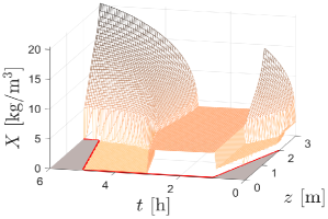
Figure 5. Example 1: simulated concentration (semi-implicit scheme, $N=100$) of total suspended solids.

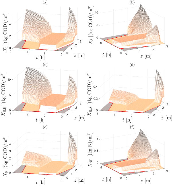
Figure 6. Example 1: simulated concentrations of solid components (semi-implicit scheme, $N=100$): (a) particulate inert organic matter, (b) slowly biodegradable substrate, (c) active heterotrophic biomass, (d) active autotrophic biomass, (e) particle products from biomass decay, (f) particulate biodegradable organic nitrogen.

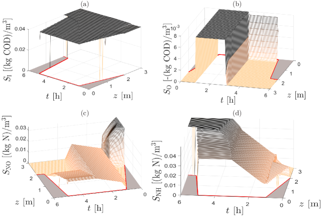
Figure 7. Example 1: simulated densities (semi-implicit scheme, $N=100$) of soluble components (part 1): (a) soluble inert organic matter, (b) oxygen, (c) nitrate and nitrite nitrogen, (d) $\mathrm{NH}_{4}^{+}\ +\ \mathrm{NH}_{3}$ nitrogen.

Figure 8. Example 1: simulated densities (semi-implicit scheme, $N=100$) of soluble components (part 2): (a, b) readily biodegradable substrate (two different views), (c, d) soluble biodegradable organic nitrogen (two different views).

It is the purpose of this example to illustrate the SBR model as a whole. (The performance of the three numerical schemes SBR2 in [6], and the explicit and semi-implicit ones here in terms of errors and efficiency is studied in Examples 2 and 3.) We simulated the five stages of an SBR as outlined in Table 1. The duration of the whole cycle of stages during a couple of hours is realistic. The results are illustrated in Figures 5 to 8, which depict the concentration profiles of total suspended solids, particulate, and soluble components within the reactor vessel, respectively.

5.2. Example 2

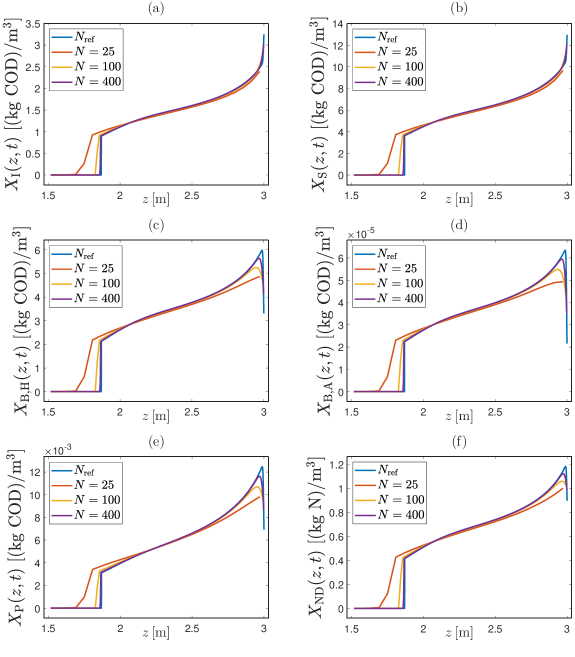
Figure 9. Example 2: simulated concentrations (semi-implicit scheme) at $T=1\,\mathrm{h}$ of solid components: (a) particulate inert organic matter, (b) slowly biodegradable substrate, (c) active heterotrophic biomass, (d) active autotrophic biomass, (e) particle products from biomass decay, (f) particulate biodegradable organic nitrogen.

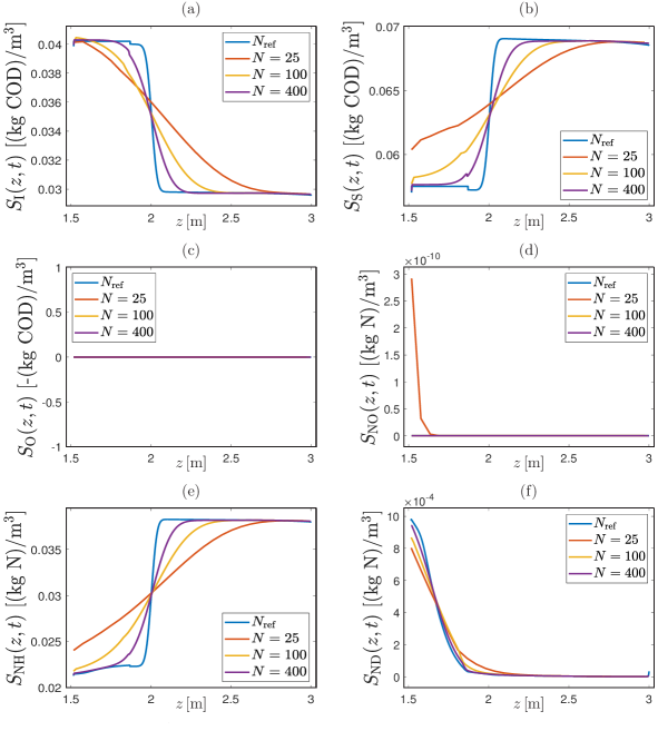
Figure 10. Example 2: simulated concentrations (semi-implicit scheme) at $T=1\,\mathrm{h}$ of soluble components: (a) soluble inert organic matter, (b) readily biodegradable substrate, (c) oxygen, (d) nitrate and nitrite nitrogen, (e) $\mathrm{NH}_{4}^{+}\ +\ \mathrm{NH}_{3}$ nitrogen, (f) soluble biodegradable organic nitrogen.

The prime motivation of this example is to study the numerical errors of the two new schemes defined for the PDE model and the scheme SBR2 of [6]. To this end we consider the scenario defined by Table 2, which refers to a shorter period of total simulated time ($T=1\,\mathrm{h}$) and does not include a react stage (for which the original SBR model, as studied in Example 1, stipulates a model by a system of ODEs). We calculated a reference solution, using the same feed conditions as in Example 1 with $N=N_{\mathrm{ref}}\coloneqq 4800$. This solution was obtained by the explicit scheme of Section 3.2. The relative approximate numerical error

$$e_{N}^{\mathrm{rel}}(t)\coloneqq\sum_{k=1}^{k_{\boldsymbol{C}}}\frac{\|C_{N}^{(k)}-C_{N_{\mathrm{ref}}}^{(k)}(\cdot,t)\|_{L^{1}(0,B)}}{\|C_{N_{\mathrm{ref}}}^{(k)}(\cdot,t)\|_{L^{1}(0,B)}}+\sum_{k=1}^{k_{\boldsymbol{S}}}\frac{\|S_{N}^{(k)}-S_{N_{\mathrm{ref}}}^{(k)}(\cdot,t)\|_{L^{1}(0,B)}}{\|S_{N_{\mathrm{ref}}}^{(k)}(\cdot,t)\|_{L^{1}(0,B)}}.$$

compares the approximate solution to the reference solution at a given time point $t$ for a specific number of cells $N$.

In Figures 9 and 10, we demonstrate the convergence of the numerical solutions, all produced with the semi-implicit scheme and a tolerance $\varepsilon=10^{-8}$, to the reference solution. That value was chosen by previous experience. The effect of the tolerance parameter $\varepsilon$ itself is studied in Table 3 for simulations done with $N=50$, $100$, and $200$, in terms of the average number of iterations during the simulation, the relative error, and CPU time. It turns out that the relative error depends only marginally on the choice of $\varepsilon$. As one should expect, the average number of iterations (of the Newton-Raphson scheme, per time step), as well as the CPU time for the whole simulation, consistently increase with decreasing $\varepsilon$. Overall, it appears that the relative error and CPU time, and therefore efficiency, does not depend critically on $\varepsilon$ (at least for the model functions and parameters chosen here).

For the same configuration, we compare in Table 4 and Figure 11 the relative errors and CPU times obtained by the three schemes SBR2 of [6], and the explicit and semi-implicit schemes of Sections 3 and 4, respectively. For both explicit and semi-implicit schemes, simulations were performed for $N=25,\dots,1600$ using the Engquist-Osher flux (3.2). The semi-implicit scheme was calculated with the tolerance $\varepsilon=10^{-8}$. It turns out that with the exception of very coarse discretizations, the semi-implicit scheme is significantly more efficient in error reduction per CPU time than its explicit counterpart due to its more favorable CFL condition, and is more efficient also than SBR2 for sufficiently fine discretizations. It is noteworthy that all schemes converge to the same solution.

Table 2. Example 2: time functions for the simulation of the reference solution.

Time period $[\mathrm{h}]$	$X_{\mathrm{f}}(t)[\rm kg/m^{3}]$	$Q_{\mathrm{f}}(t)[\rm m^{3}/h]$	$Q_{\mathrm{u}}(t)[\rm m^{3}/h]$	$Q_{\mathrm{e}}(t)[\rm m^{3}/h]$	Model
$0\ \ \leq t<0.3$	5	2660	0	0	PDE
$0.3\ \leq t<0.85$	0	0	0	0	PDE
$0.85\leq t<0.95$	0	0	0	6000	PDE
$0.95\leq t<1$	0	0	100	0	PDE

Table 3. Example 2: effect of the tolerance $\varepsilon$ on the average number of iterations in the Newton-Raphson method, the errors $e_{N}^{\mathrm{rel}}$ and CPU times during a simulation of $T=1\,\mathrm{h}$. The errors are computed with the reference solution obtained by the explicit scheme with $N=4800$ and the Godunov numerical flux.

	$\varepsilon$	Avg. iterations	$e_{N}^{\mathrm{rel}}(t)$	CPU [$\mathrm{s}$]
$N=50$	1E-1	1.00	0.0497756500328602	0.1250
	1E-2	1.03	0.0497756500328602	0.1406
	1E-3	1.60	0.0497679356628912	0.1797
	1E-4	2.00	0.0497674399512266	0.1953
	1E-5	2.01	0.0497674389897926	0.1875
	1E-6	2.04	0.0497674143163951	0.1797
	1E-7	2.12	0.0497674123749513	0.1953
	1E-8	2.77	0.0497674121051164	0.2109
	1E-9	2.92	0.0497674120899535	0.2344
	1E-10	2.96	0.0497674120878119	0.2188
	1E-11	3.07	0.0497674120875128	0.2422
	1E-12	3.69	0.0497674120874927	0.2560
$N=100$	1E-1	1.00	0.0244467141865713	0.3984
	1E-2	1.01	0.0244467141865713	0.4062
	1E-3	1.21	0.0244432794902836	0.4453
	1E-4	2.00	0.0244427209345141	0.6719
	1E-5	2.01	0.0244427236620445	0.5938
	1E-6	2.02	0.0244427043886650	0.6172
	1E-7	2.06	0.0244427032349412	0.6250
	1E-8	2.17	0.0244427031258883	0.7188
	1E-9	2.87	0.0244427030983648	0.7656
	1E-10	2.97	0.0244427030958998	0.7812
	1E-11	3.01	0.0244427030956931	0.7734
	1E-12	3.11	0.0244427030956539	0.8672
$N=200$	1E-1	1.00	0.0115032639159754	1.4609
	1E-2	1.00	0.0115032639159754	1.4766
	1E-3	1.07	0.0115029463554388	1.6406
	1E-4	1.86	0.0115009448742330	2.0234
	1E-5	2.01	0.0115008746422637	2.2578
	1E-6	2.02	0.0115008746587289	2.2188
	1E-7	2.03	0.0115008741995477	2.1250
	1E-8	2.08	0.0115008740687287	2.2656
	1E-9	2.24	0.0115008740547202	2.3281
	1E-10	2.91	0.0115008740528361	2.7812
	1E-11	3.00	0.0115008740526303	2.7812
	1E-12	3.03	0.0115008740526086	2.9609

Table 4. Example 2: errors $e_{N}^{\mathrm{rel}}$ and CPU times at simulated time $T=1\,$h. The errors have been computed with the reference solution obtained by explicit scheme with $N=4800$ and the Godunov numerical flux. The abbreviation SBR2 refers to the scheme in [6] (without variable transformation).

		SBR2		Explicit		Semi-implicit
	$N$	$e_{N}^{\mathrm{rel}}(t)$	CPU $[\mathrm{s}]$	$e_{N}^{\mathrm{rel}}(t)$	CPU $[\mathrm{s}]$	$e_{N}^{\mathrm{rel}}(t)$	CPU $[\mathrm{s}]$
$T=0.4\,\mathrm{h}$	25	1.6483	0.0391	1.2053	0.0391	1.2099	0.0469
	50	0.9230	0.0703	0.7688	0.1035	0.7732	0.0938
	100	0.4704	0.2090	0.4368	0.3340	0.4414	0.2070
	200	0.2551	0.7969	0.2384	1.7969	0.2416	0.5508
	400	0.1352	5.2441	0.1261	11.9395	0.1286	2.0234
	800	0.0743	40.9023	0.0645	89.9941	0.0665	7.4453
	1600	0.0409	316.4102	0.0379	717.4668	0.0397	27.5156
$T=0.75\,\mathrm{h}$	25	1.5691	0.0900	1.2901	0.0920	1.2959	0.0880
	50	0.8327	0.1320	0.7835	0.1590	0.7880	0.1360
	100	0.4204	0.3240	0.4392	0.4590	0.4451	0.3190
	200	0.2125	1.4766	0.2304	3.1797	0.2345	1.0234
	400	0.1103	9.5469	0.1218	20.7266	0.1250	3.6797
	800	0.0595	79.1719	0.0620	175.6562	0.0644	14.2188
	1600	0.0327	646.8438	0.0371	1421.2190	0.0392	55.6470
$T=1\,\mathrm{h}$	25	1.1617	0.0469	1.0747	0.0508	1.0573	0.0566
	50	0.6580	0.0957	0.6966	0.1191	0.7078	0.1289
	100	0.3760	0.3555	0.4519	0.6797	0.4627	0.3984
	200	0.1877	1.9004	0.2821	4.0605	0.2919	1.3066
	400	0.1075	12.4375	0.1658	27.0586	0.1737	4.8535
	800	0.0644	104.6543	0.0896	237.3340	0.0966	18.8379
	1600	0.0418	822.3809	0.0439	2362.8570	0.0495	75.5801

Figure 11. Example 2: error versus CPU time for various values of $N$ (Table 4) at simula times (a) $T=0.4\,\mathrm{h}$, (b) $T=0.75\,\mathrm{h}$ and (c) $T=1\,\mathrm{h}$; (d) simulated total suspended solids concentration ($N=4800$) during $1\,\mathrm{h}$ (reference solution).

5.3. Example 3

We investigate the impact of a moving mesh with three different spatial grids, compared to a fixed grid; see Figure 12. The simulation conditions are given in Table 5. The semi-implicit scheme is used with the Engquist-Osher flux and $\varepsilon=10^{-8}$. The data in Table 5, which contemplate no solids feed or discharge but a moving boundary, have been chosen in such a way that the solution converges quickly in time to a stationary one with a layer of sediment at the bottom produced by the settling of the initially homogeneous suspension that is not affected by the moving boundary. Figures 12 (a), (c) and (e) show that the numerical solution of the SBR2 scheme reproduces this property at any of the chosen discretizations $N=100$, $N=200$ or $N=400$ while the solution produced by the semi-implicit scheme is not stationary due to the effect of the moving mesh. The deviation from a stationary solution seems, however, to decrease with increasing $N$.

Table 5. Example 3: Time functions for the simulation.

Time period $[\mathrm{h}]$	$X_{\mathrm{f}}(t)[\rm kg/m^{3}]$	$Q_{\mathrm{f}}(t)[\rm m^{3}/h]$	$Q_{\mathrm{u}}(t)[\rm m^{3}/h]$	$Q_{\mathrm{e}}(t)[\rm m^{3}/h]$	Model
$0\leq t<25$	0	0	0	0	PDE
$25\leq t<35$	0	0	0	84	PDE
$35\leq t<45$	0	0	0	0	PDE
$45\leq t<60$	0	40	0	0	PDE
$60\leq t<70$	0	0	0	0	PDE

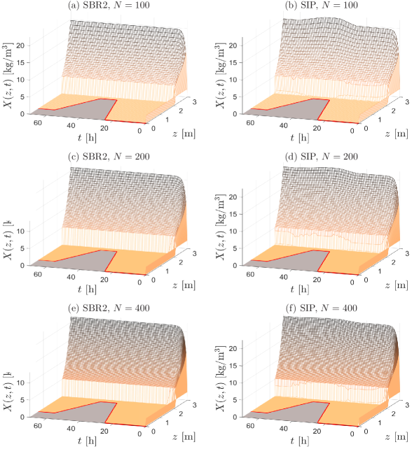
Figure 12. Example 3: simulations of the scenario of Table 5 with the indicated schemes and values of $N$. The fixed-mesh scheme SBR2 reproduces a steady-state profile while numerical solutions by scheme SIP are affected by the moving mesh.

6. Conclusions

The numerical results demonstrate that the two versions of the numerical scheme presented herein, the explicit one of Section 3.2 and the semi-implicit one of Section 4, generate physically relevant solutions (as is expressed by the invariant region principle) and are working alternatives to the scheme SBR2 in [6] of the PDE model advanced in [5]. Moreover, as Example 2 clearly illustrates, there is a substantial gain in CPU times and efficiency of the semi-implicit version if compared with the explicit version. This gain is of course due to the more favorable CFL condition (CFL-SI) (for the semi-implicit scheme) that permits a larger time step than (CFL) (for the explicit scheme). The degree of this advantage depends, of course, on the constitutive functions and parameters used, so it is important to emphasize that it appears for choices of these constitutive ingredients that are largely considered typical for activated sludge [4, 35, 7, 30].

The SBR2 scheme of [6] is based on a fixed grid with respect to $z$, and the moving interface $\bar{z}(t)$ needs to be tracked explicitly. This movement gives rise to a number of cases of boundary cells of time-dependent size that need to be handled separately. That treatment is fairly involved and the approach presented in the present work is in general easier to implement, and for the semi-implicit variant turns out to be more efficient. That said, we mention that the fixed-grid approach of [6] has certain advantages in situations when the method is required to leave a consolidated bed invariant under movements of $\bar{z}(t)$ above it (as is illustrated by Example 3), and can be extended more easily to additional inlets or outlets in the reactor. It is therefore interesting to note that the observed convergence of the three schemes discussed to the same solution, as evidenced by Table 4 and Figure 11 (a), supports that the treatment in [6] is correct.

With respect to limitations, we mention that the approach of [6] involves a vessel with variable cross-sectional area; this model ingredient has been left out here for notational convenience and is not expected to make the formulation and analysis significantly more difficult. We also note that while it has been proven that the schemes are monotone and obey an invariant-region principle and numerical evidence of convergence has been presented, a rigorous convergence proof is still missing but can possibly be obtained by combining analyses of weakly coupled degenerate parabolic systems [26], numerical methods for zero-flux boundary value problems [9, 29], and studies of triangular systems of conservation laws and degenerate convection-diffusion equations [10, 11, 18]. (In the latter reference, convergence proofs decisively depend on usage of the Engquist-Osher flux with its separable upwind and downwind contributions; this has partly motivated usage of that particular numerical flux in the present work.)

Several extensions, improvements and applications of the model and numerical methods are conceivable. For instance, both scheme versions are only first-order accurate in space and time; this order can possibly be improved by applying more sophisticated variable extrapolation or maximum-principle-preserving weighted essentially non-oscillatory (WENO) techniques (cf., e.g., [28] and references cited in that work) combined with changing between the implicit and explicit steps in a more involved manner as is done in implicit-explicit (IMEX) schemes, cf., e.g., [2]. On the other hand, one can think of an SBR whose bottom works as a filter or a filtration cell with chemical reactions. In such applications, the trajectory of $\bar{z}(t)$ is no longer prescibed but arises from an applied pressure, and is balanced by the hydraulic resistance of the filter medium plus that of the forming sediment (filter cake). The composition of the latter is part of the solution, so that possible extension forms a free-boundary problem [8, 14].

We emphasize that within the present approach soluble components are supposed to be transported passively with the fluid and are subject to the reaction terms. In some of the figure this property causes fairly sharp concentration profiles when one expects that the evolution of solute concentrations should be subject to additional effects such as dispersion/diffusion. In fact, diffusion driven by the gradient of the respective concentration was the unique mechanism of spatial propagation of solutes considered in our first effort of modelling reactive settling by PDEs [4]. It would not be a problem to include diffusion to the present approach as an additional mechanism of solute transport, with the effect to be an overall blurring of profiles.

Appendix A A modified ASM1 model

Table 6. The variables in the modified ASM1 model.

Material	Notation	Unit
Particulate inert organic matter	$X_{\rm I}$	$\rm(kg\ COD)\,m^{-3}$
Slowly biodegradable substrate less part. organic nitrogen	$X_{\rm S-ND}$	$\rm(kg\ COD)\,m^{-3}$
Active heterotrophic biomass	$X_{\rm B,H}$	$\rm(kg\ COD)\,m^{-3}$
Active autotrophic biomass	$X_{\rm B,A}$	$\rm(kg\ COD)\,m^{-3}$
Particulate products arising from biomass decay	$X_{\rm P}$	$\rm(kg\ COD)\,m^{-3}$
Particulate biodegradable organic nitrogen	$X_{\rm ND}$	$\rm(kg\ N)\,m^{-3}$
Soluble inert organic matter	$S_{\rm I}$	$\rm(kg\ COD)\,m^{-3}$
Readily biodegradable substrate	$S_{\rm S}$	$\rm(kg\ COD)\,m^{-3}$
Oxygen	$S_{\rm O}$	$\rm-(kg\ COD)\,m^{-3}$
Nitrate and nitrite nitrogen	$S_{\rm NO}$	$\rm(kg\ N)\,m^{-3}$
$\mathrm{NH}_{4}^{+}+\mathrm{NH}_{3}$ nitrogen	$S_{\rm NH}$	$\rm(kg\ N)\,m^{-3}$
Soluble biodegradable organic nitrogen	$S_{\rm ND}$	$\rm(kg\ N)\,m^{-3}$

Table 7. Stoichiometric and kinetic parameters.

Symbol	Name	Value	Unit
$Y_{\rm A}$	Yield for autotrophic biomass	0.24	$\rm(g\,COD)(g\,N)^{-1}$
$Y_{\rm H}$	Yield for heterotrophic biomass	0.67	$\rm(g\,COD)(g\,COD)^{-1}$
$f_{\rm P}$	Fraction of biomass leading to particulate products	0.08	dimensionless
$i_{\rm XB}$	Mass of nitrogen per mass of COD in biomass	0.086	$\rm(g\,N)(g\,COD)^{-1}$
$i_{\rm XP}$	Mass of nitrogen per mass of COD in products from biomass	0.06	$\rm(g\,N)(g\,COD)^{-1}$
$\mu_{\rm H}$	Maximum specific growth rate for heterotrophic biomass	6.0	$\rm d^{-1}$
$K_{\rm S}$	Half-saturation coefficient for heterotrophic biomass	20.0	$\rm(g\,COD)\,m^{-3}$
$K_{\rm O,H}$	Oxygen half-saturation coefficient for heterotrophic biomass	0.2	$\rm-(g\,COD)\,m^{-3}$
$K_{\rm NO}$	Nitrate half-saturation coefficient for denitrifying heterotrophic biomass	0.5	$\rm(g\,NO_{3}\text{-}N)\,m^{-3}$
$b_{\rm H}$	Decay coefficient for heterotrophic biomass	0.62	$\rm d^{-1}$
$\eta_{\rm g}$	Correction factor for $\mu_{\rm H}$ under anoxic conditions	0.8	dimensionless
$\eta_{\rm h}$	Correction factor for hydrolysis under anoxic conditions	0.4	dimensionless
$k_{\rm h}$	Maximum specific hydrolysis rate	3.0	$\rm(g\,\text{COD})\,(g\,\text{COD})^{-1}\rm d^{-1}$
$K_{\rm X}$	Half-saturation coefficient for hydrolysis of slowly biodegradable substrate	0.03	$\rm(g\,\text{COD})(g\,\text{COD})^{-1}$
$\mu_{\rm A}$	Maximum specific growth rate for autotrophic biomass	0.8	$\rm d^{-1}$
$\bar{K}_{\rm NH}$	Ammonia half-saturation coefficient for aerobic and anaerobic growth of heterotrophs	0.05	$\rm(g\,NH_{3}\text{-}N)\,m^{-3}$
$K_{\rm NH}$	Ammonia half-saturation coefficient for autotrophic biomass	1.0	$\rm(g\,NH_{3}\text{-}N)\,m^{-3}$
$b_{\rm A}$	Decay coefficient for autotrophic biomass	0.15	$\rm d^{-1}$
$K_{\rm O,A}$	Oxygen half-saturation coefficient for autotrophic biomass	0.4	$\rm-(g\,COD)\,m^{-3}$
$k_{\rm a}$	Ammonification rate	0.08	$\rm m^{3}(g\,COD)^{-1}d^{-1}$

The ASM1 model is described in, for example,  [25]. For the reason of reformulating the PDE model to include percentages of the particulate concentrations, we have redefined the second component from $X_{\mathrm{S}}$ to $X_{\mathrm{S-ND}}\coloneqq X_{\mathrm{S}}-X_{\mathrm{ND}}$. Then the variables are

$$\boldsymbol{C}=\big{(}X_{\mathrm{I}},X_{\mathrm{S-ND}},X_{\mathrm{B,H}},X_{\mathrm{B,A}},X_{\mathrm{P}},X_{\rm ND}\big{)}^{\mathrm{T}},\quad\boldsymbol{S}=\big{(}S_{\mathrm{I}},S_{\mathrm{S}},S_{\mathrm{O}},S_{\mathrm{NO}},S_{\mathrm{NH}},S_{\mathrm{ND}}\big{)}^{\mathrm{T}},$$

with units given in Table 6. The stoichiometric matrices of the modified ASM1 are given by

$$\boldsymbol{\sigma}_{\mathrm{\!\boldsymbol{C}}}\coloneqq\begin{bmatrix}0&0&0&0&0&0&0&0\\ 0&0&0&1-f_{\rm P}(1+i_{\rm XP})-i_{\rm XB}&1-f_{\rm P}(1+i_{\rm XP})-i_{\rm XB}&0&-1&1\\ 1&1&0&-1&0&0&0&0\\ 0&0&1&0&-1&0&0&0\\ 0&0&0&f_{\rm P}&f_{\rm P}&0&0&0\\ 0&0&0&i_{\rm XB}-f_{\rm P}i_{\rm XP}&i_{\rm XB}-f_{\rm P}i_{\rm XP}&0&0&-1\end{bmatrix}$$

for the solid components and

$$\boldsymbol{\sigma}_{\mathrm{\!\boldsymbol{S}}}\coloneqq\begin{bmatrix}0&0&0&0&0&0&0&0\\ -1/Y_{\rm H}&-1/Y_{\rm H}&0&0&0&0&1&0\\ -(1-Y_{\rm H})/Y_{\rm H}&0&-(4.57-Y_{\rm A})/Y_{\rm A}&0&0&0&0&0\\ 0&-(1-Y_{\rm H})/(2.86Y_{\rm H})&1/Y_{\rm A}&0&0&0&0&0\\ -i_{\rm XB}&-i_{\rm XB}&-i_{\rm XB}-1/Y_{\rm A}&0&0&1&0&0\\ 0&0&0&0&0&-1&0&1\end{bmatrix}$$

for the substrates, where the constants are given in Table 7 and the vector of reaction rates is

$$\boldsymbol{r}(\boldsymbol{C},\boldsymbol{S})\coloneqq\begin{pmatrix}\mu_{\rm H}\mu(S_{\rm NH},\bar{K}_{\rm NH})\mu(S_{\rm S},K_{\rm S})\mu(S_{\rm O},K_{\rm O,H})X_{\rm B,H}\\[2.0pt] \mu_{\rm H}\mu(S_{\rm NH},\bar{K}_{\rm NH})\mu(S_{\rm S},K_{\rm S})\mu(K_{\rm O,H},S_{\rm O})\mu(S_{\rm NO},K_{\rm NO})\eta_{\rm g}X_{\rm B,H}\\[2.0pt] \mu_{\rm A}\mu(S_{\rm NH},K_{\rm NH})\mu(S_{\rm O},K_{\rm O,A})X_{\rm B,A}\\[2.0pt] b_{\rm H}X_{\rm B,H}\\[2.0pt] b_{\rm A}X_{\rm B,A}\\[2.0pt] k_{\rm a}S_{\rm ND}X_{\rm B,H}\\[2.0pt] k_{\rm h}\mu_{7}(X_{\rm S},X_{\rm B,H})\bigl{(}\mu(S_{\rm O},K_{\rm O,H})+\eta_{\rm h}\mu(K_{\rm O,H},S_{\rm O})\mu(S_{\rm NO},K_{\rm NO})\bigr{)}\\[2.0pt] k_{\rm h}\mu_{8}(X_{\rm B,H},X_{\rm ND})\bigl{(}\mu(S_{\rm O},K_{\rm O,H})+\eta_{\rm h}\mu(K_{\rm O,H},S_{\rm O})\mu(S_{\rm NO},K_{\rm NO})\bigr{)}\end{pmatrix}.$$

Here we define the Monod expression $\mu(A,B):=A/(A+B)$ and

$$\mu_{7}(X_{\rm S},X_{\rm B,H}) \coloneqq\begin{cases}0&\text{if $X_{\rm S}=0$ and $X_{\rm B,H}=0$,}\\ \dfrac{X_{\rm S}X_{\rm B,H}}{K_{\rm X}X_{\rm B,H}+X_{\rm S}}&\text{otherwise,}\end{cases}$$

$$\mu_{8}(X_{\rm B,H},X_{\rm ND}) \coloneqq\begin{cases}0&\text{if $X_{\rm S}=0$ and $X_{\rm B,H}=0$,}\\ \dfrac{X_{\rm B,H}X_{\rm ND}}{K_{\rm X}X_{\rm B,H}+X_{\rm S}}&\text{otherwise.}\end{cases}$$

References

- [1] M. M. Amin, M. H. Khiadani (Hajian), A. Fatehizadeh, and E. Taheri. Validation of linear and non-linear kinetic modeling of saline wastewater treatment by sequencing batch reactor with adapted and non-adapted consortiums. Desalination, 344:228–235, July 2014.
- [2] S. Boscarino, R. Bürger, P. Mulet, G. Russo, and L. M. Villada. Linearly implicit IMEX Runge-Kutta methods for a class of degenerate convection-diffusion problems. SIAM J. Sci. Comput., 37(2):B305–B331, 2015.
- [3] R. Bürger, J. Careaga, and S. Diehl. A method-of-lines formulation for a model of reactive settling in tanks with varying cross-sectional area. IMA J. Appl. Math., 86(3):514–546, 2021.
- [4] R. Bürger, J. Careaga, S. Diehl, C. Mejías, I. Nopens, E. Torfs, and P. A. Vanrolleghem. Simulations of reactive settling of activated sludge with a reduced biokinetic model. Computers Chem. Eng., 92:216–229, 2016.
- [5] R. Bürger, J. Careaga, S. Diehl, and R. Pineda. A moving-boundary model of reactive settling in wastewater treatment. Part 1: Governing equations. Appl. Math. Modelling, 106:390–401, 2022.
- [6] R. Bürger, J. Careaga, S. Diehl, and R. Pineda. A moving-boundary model of reactive settling in wastewater treatment. Part 2: Numerical scheme. Appl. Math. Modelling, 111:247–269, 2022.
- [7] R. Bürger, J. Careaga, S. Diehl, and R. Pineda. A model of reactive settling of activated sludge: Comparison with experimental data. Chem. Eng. Sci., 267:118244, Mar. 2023.
- [8] R. Bürger, F. Concha, and K. H. Karlsen. Phenomenological model of filtration processes: 1. Cake formation and expression. Chem. Eng. Sci., 56:4537–4553, 2001.
- [9] R. Bürger, A. Coronel, and M. Sepúlveda. A semi-implicit monotone difference scheme for an initial-boundary value problem of a strongly degenerate parabolic equation modeling sedimentation-consolidation processes. Math. Comp., 75(253):91–112, 2006.
- [10] R. Bürger, S. Diehl, M. C. Martí, and Y. Vásquez. A degenerating convection-diffusion system modelling froth flotation with drainage. IMA J. Appl. Math., 87(6):1151–1190, 2022.
- [11] R. Bürger, S. Diehl, M. C. Martí, and Y. Vásquez. A difference scheme for a triangular system of conservation laws with discontinuous flux modeling three-phase flows. Netw. Heterog. Media, 18:140–190, 2023.
- [12] R. Bürger, S. Diehl, and C. Mejías. A difference scheme for a degenerating convection-diffusion-reaction system modelling continuous sedimentation. ESAIM: Math. Modelling Num. Anal., 52(2):365–392, 2018.
- [13] R. Bürger, S. Diehl, and I. Nopens. A consistent modelling methodology for secondary settling tanks in wastewater treatment. Water Res., 45(6):2247–2260, 2011.
- [14] R. Bürger, H. Frid, and K. H. Karlsen. On a free boundary problem for a strongly degenerate quasi-linear parabolic equation with an application to a model of pressure filtration. SIAM J. Math. Anal., 34(3):611–635, 2002.
- [15] R. Bürger, K. H. Karlsen, and J. D. Towers. A model of continuous sedimentation of flocculated suspensions in clarifier-thickener units. SIAM J. Appl. Math., 65:882–940, 2005.
- [16] M. Caluwé, D. Daens, R. Blust, L. Geuens, and J. Dries. The sequencing batch reactor as an excellent configuration to treat wastewater from the petrochemical industry. Water Sci. Tech., 75(4):793–801, Dec. 2016.
- [17] G. Chen, M. C. M. van Loosdrecht, G. A. Ekama, and D. Brdjaniovic. Biological Wastewater Treatment. IWA Publishing, London, UK, second edition, 2020.
- [18] G. M. Coclite, S. Mishra, and N. H. Risebro. Convergence of an Engquist-Osher scheme for a multi-dimensional triangular system of conservation laws. Math. Comp., 79:71–94, 2010.
- [19] K. Deimling. Nonlinear Functional Analysis. Springer-Verlag, Berlin, 1985.
- [20] S. Diehl. Continuous sedimentation of multi-component particles. Math. Meth. Appl. Sci., 20:1345–1364, 1997.
- [21] R. Droste and R. Gear. Theory and Practice of Water and Wastewater Treatment. Wiley, Hoboken, NJ, USA, 2nd edition, 2019.
- [22] B. Engquist and S. Osher. One-sided difference approximations for nonlinear conservation laws. Math. Comp., 36(154):321–351, 1981.
- [23] S. Evje and K. H. Karlsen. Degenerate convection-diffusion equations and implicit monotone difference schemes. In Hyperbolic Problems: Theory, Numerics, Applications, Vol. I (Zürich, 1998), volume 129 of Internat. Ser. Numer. Math., pages 285–294. Birkhäuser, Basel, 1999.
- [24] R. Eymard, T. Gallouët, and R. Herbin. Finite volume methods. In Handbook of Numerical Analysis, Vol. VII, Handb. Numer. Anal., VII, pages 713–1020. North-Holland, Amsterdam, 2000.
- [25] M. Henze, W. Gujer, T. Mino, and M. C. M. van Loosdrecht. Activated Sludge Models ASM1, ASM2, ASM2d and ASM3. IWA Publishing, London, UK, 2000. IWA Scientific and Technical Report No. 9.
- [26] H. Holden, K. H. Karlsen, and N. H. Risebro. On uniqueness and existence of entropy solutions of weakly coupled systems of nonlinear degenerate parabolic equations. Electron. J. Differential Equations, page 46, 2003.
- [27] Z. Hu, R. A. Ferraina, J. F. Ericson, A. A. MacKay, and B. F. Smets. Biomass characteristics in three sequencing batch reactors treating a wastewater containing synthetic organic chemicals. Water Res., 39(4):710–720, Feb. 2005.
- [28] Y. Jiang and Z. Xu. Parametrized maximum principle preserving limiter for finite difference WENO schemes solving convection-dominated diffusion equations. SIAM J. Sci. Comput., 35(6):A2524–A2553, 2013.
- [29] K. H. Karlsen and J. D. Towers. Convergence of monotone schemes for conservation laws with zero-flux boundary conditions. Adv. Appl. Math. Mech., 9(3):515–542, 2017.
- [30] G. Kirim, E. Torfs, and P. . A. Vanrolleghem. An improved 1d reactive Bürger–Diehl settler model for secondary settling tank denitrification. Water Environ. Res., 94:e10825, 2022.
- [31] J. Makinia and E. Zaborowska. Mathematical Modelling and Computer Simulation of Activated Sludge Systems. IWA Publishing, London, UK, 2nd edition, 2020.
- [32] L. Metcalf and H. P. Eddy. Wastewater Engineering. Treatment and Resource Recovery. McGraw-Hill, New York, USA, 5th edition, 2014.
- [33] T. Popple, J. Williams, E. May, G. Mills, and R. Oliver. Evaluation of a sequencing batch reactor sewage treatment rig for investigating the fate of radioactively labelled pharmaceuticals: Case study of propranolol. Water Res., 88:83–92, Jan. 2016.
- [34] B. Song, Z. Tian, R. van der Weijden, C. Buisman, and J. Weijma. High-rate biological selenate reduction in a sequencing batch reactor for recovery of hexagonal selenium. Water Res., 193:116855, Apr. 2021.
- [35] E. Torfs, S. Balemans, F. Locatelli, S. Diehl, R. Bürger, J. Laurent, P. François, and I. Nopens. On constitutive functions for hindered settling velocity in 1-d settler models: Selection of appropriate model structure. Water Res., 110:38–47, 2017.
- [36] S. Wang and C. K. Gunsch. Effects of selected pharmaceutically active compounds on treatment performance in sequencing batch reactors mimicking wastewater treatment plants operations. Water Res., 45(11):3398–3406, May 2011.