[orcid=0000-0003-4508-3172] Conceptualisation of this study, Methodology, Writing

[orcid=0000-0003-0637-6028] url]https://www.gagolewski.com [1] [cor1]Corresponding author Conceptualisation of this study, Methodology, Data Curation, Investigation, Software, Writing

[orcid=0000-0002-9391-6477] URL]http://if.pw.edu.pl/ siudem Conceptualisation of this study, Methodology, Writing

[orcid=0000-0002-2869-7300] Data Curation, Investigation, Visualisation, Software, Writing

Equivalence of inequality indices: Three dimensions of impact revisited

1 Introduction

Given a series of measurements, indicators, scores, counts, or any other numeric values, it is natural to order them from the highest to the lowest. This way, we get better insight into the aspects of reality they are trying to capture. In particular, various rankings (e.g., of universities, movies, or restaurants; see Iñiguez et al., 2022) aim to make our lives easier by claiming they can separate seeds from the chaff. Analysis or prediction of the size of the top or otherwise extreme values (e.g., Voitalov et al., 2019; Pickands III, 1975; Marshall and Olkin, 2007) is crucial in risk analysis or disaster prevention. The search for patterns and universalities in sorted data Holme (2022); Newman (2005) remains a fundamental, multidisciplinary research topic. This includes the study of ranking dynamics Iñiguez et al. (2022) and the distribution of their static snapshots, from the most straightforward Zipf power-law models Newman (2005) to more complex ones Petersen et al. (2011); Siudem et al. (2020, 2022); Singh et al. (2022).

Different systems or environments naturally have different sizes and levels of inequality Cowell (2000); Silber (2012), i.e., what percentage of the top scorers is in possession of the majority of the resources. As the degree of evenness vs monopoly can be measured by different indicators (e.g., the Gini, Bonferroni, or Hover index), a question arises which one is the most informative.

Furthermore, we would like to understand why inequality naturally arises as a consequence of the natural evolution of any system. Studying simple mathematical models governed by intuitive assumptions can bring many insights into this problem.

In this work, we revisit the recently-proposed 3DI model (three dimensions of impact; Siudem et al., 2020, 2022), which can be considered a rank-size approach to the problem of describing the mechanisms governing the growth of bibliographic and other networks studied originally by Price (1965).

Namely, consider a process where, in every time step, a system (e.g., a citation network, a cluster of internet portals) grows by one entity (e.g., a new paper, a website). In each iteration, we distribute $m$ impact/wealth units (e.g., citations, links) amongst the already-existing entities:

• $a=(1-\rho)m$ units totally at random,

• $p=\rho m$ units according to the preferential attachment rule,

with $\rho$ representing the extent to which the rich-get-richer rule dominates over pure luck. Inspired by the observation in Bertoli-Barsotti (2023), in Section 2, we will show that the $\rho$ parameter naturally corresponds to the value of the Gini index of the resulting ordered sample of impact measures. We will thus indicate the relationship between the degree of randomness and inequality. Furthermore, in Section 3, we will re-express some other popular inequality indices in terms of monotone, 1-to-1 functions of the Gini index, hence showing their equivalence in our model. In Section 4, an analysis of a large database of citations to research papers in economics (RePEc) will confirm our theoretical derivations. We will reach similar conclusions by analysing countrywise income data in Section 5.

2 The Gini-stable process, rich-get-richer, and random distribution of wealth

We utilise the following notation. The gamma function is given by $\Gamma(z)=\int_{0}^{\infty}t^{z-1}e^{-t}\,dt$, $\Gamma(z+1)=z\Gamma(z)$, the polygamma functions are defined by $\psi^{(m)}(z)=\frac{d^{m+1}}{dz^{m+1}}\log\left(\Gamma(z)\right)$, in particular, the digamma function is $\psi(z)=\psi^{(0)}(z)=\Gamma^{\prime}(z)/\Gamma(z)$, the Lambert $\mathcal{W}$ function (we always use the principal branch) is the solution of the equation $\mathcal{W}(z)\exp\left[\mathcal{W}(z)\right]=z$, the harmonic number $H_{k}=\psi(k+1)-\gamma$, where $\gamma\approx 0.577$ is the Euler constant.

For any fixed parameter $G\in[0,1)$, consider an iterative process discussed in (Bertoli-Barsotti et al., 2023) whose update formula features a simple affine function of the consecutive elements:

$$p_{k}^{(N,G)}=a_{N}(G)+b_{N}(G)\,p_{k}^{(N-1,G)},\qquad k=1,\dots,N,$$ (1)

for $N\geq 2$, under the assumption that $p_{N}^{(N-1,G)}=0$ and $p_{1}^{(1,G)}=1$ and:

$$a_{N}(G) = \frac{1-G}{G(N-2)+1}\frac{1}{N},$$ (2)

$$b_{N}(G) = \frac{G(N-1)}{G(N-2)+1}.$$ (3)

Then, for any $N\geq 2$, $\boldsymbol{p}^{(N,G)}=\left(p_{1}^{(N,G)},\dots,p_{N}^{(N,G)}\right)$ is an ordered probability $N$-vector, i.e., $\sum_{k=1}^{N}p_{k}^{(N,G)}=1$ and $1\geq p_{1}^{(N,G)}\geq p_{2}^{(N,G)}\geq\dots\geq p_{N}^{(N,G)}\geq 0$.

Example 1.

Here are two example outcomes for $G=0.25$ and $G=0.75$ up to $N=4$:

	$\boldsymbol{p}^{(N,0.25)}$	$\boldsymbol{p}^{(N,0.75)}$
$N=2$	$(0.625,0.375)$	$(0.875,0.125)$
$N=3$	$(0.450,0.350,0.200)$	$(0.798,0.155,0.048)$
$N=4$	$(0.350,0.300,0.225,0.125)$	$(0.743,0.164,0.068,0.025)$

Exact formula.

There exists an explicit formula for the individual components of the probability vectors. Namely, we can show that:

$$p_{k}^{(N,G)}=\begin{cases}\displaystyle\frac{1}{N}\frac{1-G}{2G-1}\left(\frac{\Gamma(N+1)}{\Gamma(N+1+1/G-2)}\frac{\Gamma(k+1/G-2)}{\Gamma(k)}-1\right),&\text{if }G\neq\frac{1}{2},\\ \displaystyle\frac{1}{N}\left(H_{N}-H_{k-1}\right)=\frac{1}{N}\sum_{i=k}^{N}\frac{1}{i},&\text{if }G=\frac{1}{2},\\ \end{cases}$$ (4)

where $\Gamma$ is the gamma function and $H_{N}=\sum_{i=1}^{N}\frac{1}{i}$ is the $N$-th harmonic number.

Gini index is exactly $G$.

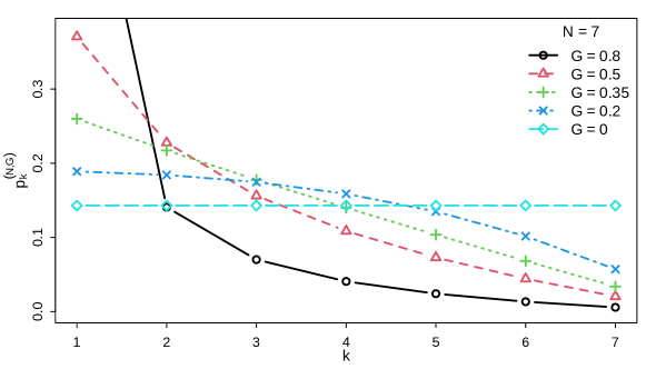
Figure 1 depicts a few example probability vectors $\boldsymbol{p}^{(7,G)}$ for different $G$s. We see that the $G$ parameter controls the level of inequality of the data distribution: $G=0$ yields all elements equal to $1/N$, and, as $G\to 1$, all probability mass is transferred to the first element.

Figure 1: Example ordered probability $N$-vectors generated using the affine update formula given by Eq. (1). Parameter $G$ controls the level of inequality, as measured by the Gini index.

It turns out that our process generates ordered probability vectors whose Gini’s index, $\mathcal{G}\left(\boldsymbol{p}^{(N,G)}\right)$ (Gini, 1912; see also, e.g., Yitzhaki and Schechtman, 2013), is equal to exactly $G$, i.e., for $N\geq 2$ and $G\neq\frac{1}{2}$ we have:

$$\mathcal{G}\left(p_{1}^{(N,G)},\dots,p_{N}^{(N,G)}\right) = \frac{1}{N-1}\sum_{k=1}^{N}(N-2k+1)p_{k}^{(N,G)}$$

$$= \displaystyle\frac{1-G}{(N-1)(2G-1)}\frac{G(2G-1)(N-1)}{1-G}=G,$$

and for $G=\frac{1}{2}$ it holds:

$$\mathcal{G}\left(p_{1}^{(N,1/2)},\dots,p_{N}^{(N,1/2)}\right)=\frac{(N-1)N}{2(N-1)N}=\frac{1}{2}.$$

Thus, quite remarkably, $N$ (size) and $G$ (inequality) are two independent parameters in our model.

Therefore, from now on, we refer to the above as the Gini-stable process; compare (Bertoli-Barsotti et al., 2023).

It is the only affine process of this kind.

Our process transforms an ordered probability vector to a new, longer, ordered probability vector of the same Gini index. What is more, the aforementioned coefficients $a_{N}$ and $b_{N}$ make up the only affine transformation that achieves this property.

Proposition 1.

For any $N\geq 3$ and $G\in[0,1)$, let $\boldsymbol{q}^{(N-1)}$ be an ordered probability $(N-1)$-vector with the Gini index of $\mathcal{G}\left(q_{1}^{(N-1)},\dots,q_{N-1}^{(N-1)}\right)=G$. Then, generating the probability $N$-vector $\boldsymbol{q}^{(N)}$ using the update formula given by Eq. (1) yields $\mathcal{G}\left(q_{1}^{(N)},\dots,q_{N}^{(N)}\right)=G$ if and only if $a_{N}$ and $b_{N}$ are given exactly by Eq. (2) and Eq. (3), respectively.

Proof.

We have $\mathcal{G}\left(q_{1}^{(N-1)},\dots,q_{N-1}^{(N-1)}\right)=\frac{1}{N-2}\sum_{k=1}^{N-1}(N-2k)q_{k}^{(N-1)}=G$. Moreover,

$$\mathcal{G}\left(q_{1}^{(N)},\dots,q_{N}^{(N)}\right) = \frac{1}{N-1}\sum_{k=1}^{N}(N-2k+1)q_{k}^{(N)}$$

$$= \frac{1}{N-1}\sum_{k=1}^{N}(N-2k+1)(a_{N}+b_{N}q_{k}^{(N-1)})$$

$$= \frac{a_{N}}{N-1}\sum_{k=1}^{N}(N-2k+1)+\frac{b_{N}}{N-1}\sum_{k=1}^{N-1}(N-2k+1)q_{k}^{(N-1)}$$

$$= 0+\frac{b_{N}}{N-1}\sum_{k=1}^{N-1}(N-2k)q_{k}^{(N-1)}+\frac{b_{N}}{N-1}$$

$$= b_{N}\left(\frac{N-2}{N-1}G+\frac{1}{N-1}\right)$$

is equal to $G$ if and only if $b_{N}=\frac{G(N-1)}{G(N-2)+1}$, which is exactly Eq. (3).

We also need to have $\sum_{k=1}^{N}p_{k}^{(N)}=1$. But after some simple transformations, we can show that this holds if and only if $a_{N}=(1-b_{N})/N$, which corresponds to Eq. (2), QED. ∎

Relation to the 3DI model.

To strengthen the underlying fundaments further, let us return to the 3DI (three dimensions of impact) model (Siudem et al., 2020) mentioned in the introduction. Let $X_{k}(t)$ denote the impact of the $k$-th richest entity at time step $t$ (e.g., the number of citations to the $k$-th most cited paper). We assume ${X}_{k}(k-1)=0$ for every $k$, i.e., the $k$-th object enters the system with no impact units. The update formula in our model is a mixture of the accidental and rich-get-richer components governed by the $\rho$ parameter:

$${X}_{k}{(t)}=\underbrace{{X}_{k}{(t-1)}}_{\mathrm{previous\;value}}+\underbrace{\frac{a}{t}}_{\mathrm{accidental\;income}}+\underbrace{p\,\frac{{X}_{k}{(t-1)}+\frac{a}{t}}{(t-1)m+a}}_{\mathrm{preferential\;gain\;or\;loss}},$$ (5)

where $a=(1-\rho)m$ and $p=\rho m$.

First, if we assume $\rho=0$, then we are only left with the accidental component, and our model reduces to the harmonic one (compare Cena et al., 2022):

$${X}_{k}(t)=m\sum\limits_{i=k}^{t}\frac{1}{i}=m\left(H_{t}-H_{k-1}\right).$$

Note that “purely accidental” does not mean that every entity ends up with the same amount of wealth, as older agents have had more opportunities to become impactful (“the old get richer”).

For $\rho<1$ and $\rho\neq 0$, the solution is:

$$X_{k}(t) = m\frac{1-\rho}{\rho}\displaystyle\left(\frac{\Gamma(t+1)}{\Gamma(t+1-\rho)}\frac{\Gamma(k-\rho)}{\Gamma(k)}-1\right)$$ (6)

$$= m\frac{1-\frac{1}{2-\rho}}{\frac{2}{2-\rho}-1}\displaystyle\left(\frac{\Gamma(t+1)}{\Gamma\left[t-1+(2-\rho)\right]}\frac{\Gamma\left[k-2+(2-\rho)\right]}{\Gamma(k)}-1\right).$$

We, therefore, note that:

$$X_{k}(t)=mtp_{k}^{(t,G)}$$ (7)

with:

$$\rho(G)=2-\frac{1}{G}=\frac{2G-1}{G},$$

or, equivalently:

$$G(\rho)=\frac{1}{2-\rho},$$

and $p_{k}^{(t,G)}$ given by Eq. (1).

We have thus established a beautiful connection between the 3DI model (Siudem et al., 2020) and the Gini-stable process Bertoli-Barsotti et al. (2023), and hence the degree of randomness in the impact distribution and the Gini index. Let us also note that in (Bertoli-Barsotti et al., 2023), where we have studied the asymptotic behaviour of the Lorenz curves generated by this model, we have also shown its relationship to the Type II Pareto, exponential, and scaled beta distributions (compare Arnold, 2015; Pickands III, 1975; Marshall and Olkin, 2007), extending the results from (Siudem et al., 2022).

3 Measuring Inequality

Majorisation order.

Given two $N$-vectors $\boldsymbol{p}$ and $\boldsymbol{p}^{\prime}$ with $\sum_{i=1}^{N}p_{i}=\sum_{i=1}^{N}p_{i}^{\prime}$, we define the majorisation order $\preceq$ (Marshall et al., 2011) in such a way that $\boldsymbol{p}\preceq\boldsymbol{p}^{\prime}$ if and only if for all $k=1,\dots,N$ it holds $F_{k}\leq F_{k}^{\prime}$, where $F_{k}=\sum_{i=1}^{k}p_{[i]}$ and $F_{k}^{\prime}=\sum_{i=1}^{k}p_{[i]}^{\prime}$ are the sums of the $k$ greatest elements in $\boldsymbol{p}$ and $\boldsymbol{p}^{\prime}$, respectively. In other words, it is the extension of the standard componentwise relation, $\leq$, applied over the consecutive cumulative sums of ordered items.

Let us note that such cumulative sums in our model can be expressed using the following simple formula:

$$F_{k}^{(N,G)}=\sum_{i=1}^{k}p_{i}^{(N,G)}=\begin{cases}\displaystyle\frac{1-G}{2G-1}\left(\frac{G}{1-G}\frac{\Gamma(N)}{\Gamma(N-1+1/G)}\frac{\Gamma(k-1+1/G)}{\Gamma(k)}-\frac{k}{N}\right),&\text{if }G\neq\frac{1}{2},\\ \displaystyle\frac{k}{N}\left(1+H_{N}-H_{k}\right),&\text{if }G=\frac{1}{2}.\\ \end{cases}$$ (8)

Monotonicity w.r.t. the majorisation order.

We can show that for any $N$, $\boldsymbol{p}^{(N,G)}$ as a function of $G$ is monotone with respect to the majorisation order.

Theorem 1.

For any $G\leq G^{\prime}$ and $N$, it holds $\boldsymbol{p}^{(N,G)}\preceq\boldsymbol{p}^{(N,G^{\prime})}$.

See Bertoli-Barsotti et al. (2023) for the proof, where we discuss the Gini-stable process in the context of the more general Lorenz ordering.

Inequality indices.

Let us now consider any function $\phi$ that maps the ordered probability $N$-vectors to the set of real numbers. We say that $\phi$ is Schur-convex, if for any $\boldsymbol{p}\preceq\boldsymbol{p}^{\prime}$ it holds ${\phi}(\boldsymbol{p})\leq{\phi}(\boldsymbol{p}^{\prime})$. This is equivalent to $\phi$ being increasing in each $F_{1},\dots,F_{k}$ when re-expressed in terms of cumulative sums of ordered elements; see Beliakov et al. (2016).

Any Schur-convex function normalised such that $\phi(1,0,\dots,0)=1$ and $\phi(1/N,\dots,1/N)=0$ is called an inequality index; see Shorrocks and Foster (1987) and (Marshall et al., 2011; Lambert, 2001; Chantreuil and Trannoy, 2011; Zheng, 2007; Bosmans, 2016).

The Gini index is an example function fulfilling these properties. Below we recall some other noteworthy inequality indices (compare, e.g., Ciommi et al., 2022; Mehran, 1976; Imedio-Olmedo et al., 2012; McVinish and Lester, 2020; Beliakov et al., 2016). Then, we derive the formulae for different inequality indices as functions of $N$ and $G$ in our model. This will enable us to express every index as a function of any another one.

Bonferroni’s index.

For any probability $N$-vector, the Bonferroni index (Bonferroni, 1930) is given by:

$$\mathcal{B}(p_{1},\dots,p_{N})= \frac{N\sum_{i=1}^{N}\left(1-\sum_{j=1}^{i}\frac{1}{N-j+1}\right)p_{i}}{N-1}=\frac{N\sum_{i=1}^{N-1}\frac{1}{N-i}\sum_{j=1}^{i}p_{j}}{N-1}-N+\frac{N}{N-1}\sum_{i=1}^{N}\left(1-\frac{1}{N-i+1}\right)$$

$$= \frac{N\sum_{i=1}^{N}\frac{1}{i}\sum_{j=1}^{N-i}p_{j}}{N-1}+\frac{N\left(1-\sum_{j=1}^{N}\frac{1}{j}\right)}{N-1}=\frac{N}{N-1}\left(\sum_{k=1}^{N-1}\frac{F_{k}}{N-k}+1-H_{N}\right).$$

Substituting $F_{k}=F_{k}^{(N,G)}$ from Eq. (8) for $\frac{1}{2}\neq G\in(0,1)$, we get:

$$\mathcal{B}\left(\boldsymbol{p}^{(N,G)}\right)= \frac{N}{(N-1)(2G-1)}\left(G\sum_{k=1}^{N-1}\frac{\Gamma(N)\Gamma(k-1+1/G)}{(N-k)\Gamma(N-1+1/G)\Gamma(k)}-\frac{1-G}{N}\sum_{k=1}^{N-1}\frac{k}{N-k}+1-H_{N}\right)$$

$$= \frac{N}{N-1}\left[\frac{G}{2G-1}\left(H_{N+1/G-2}-H_{1/G-1}\right)-\frac{1-G}{(2G-1)N}\left(NH_{N-1}-N+1\right)+1-H_{N}\right]$$

$$= \frac{N}{N-1}\left[\frac{G}{2G-1}\left(H_{N+1/G-2}-H_{1/G-1}\right)-\frac{1-G}{2G-1}\left(H_{N}-1\right)+1-H_{N}\right]$$

$$= \frac{N}{N-1}\frac{G}{2G-1}\left(H_{N+1/G-2}-H_{1/G-1}-H_{N}+1\right)$$

$$= \frac{N}{N-1}\sum_{k=2}^{N}\frac{1}{k(k+1/G-2)}.$$

For $G=\frac{1}{2}$, we get:

$$\mathcal{B}\left(\boldsymbol{p}^{(N,1/2)}\right)=\frac{N}{N-1}\sum_{k=2}^{N}\frac{1}{k^{2}}.$$

Remark 1.

Unlike in the Gini index’s case, the Bonferroni index depends on the vector length $N$. However, in the limit as $N\to\infty$, we have:

$$\mathcal{B}\left(\boldsymbol{p}^{(N,G)}\right)\stackrel{{\scriptstyle N\to\infty}}{{\longrightarrow}}\begin{cases}\displaystyle\frac{G}{2G-1}\left(1-H_{1/G-1}\right),&\mathrm{for\;}G\neq\frac{1}{2},\\ \quad\\ \displaystyle\frac{\pi^{2}-6}{6},&\mathrm{for\;}G=\frac{1}{2}.\\ \end{cases}$$

De Vergottini’s index.

The De Vergottini index Vergottini (1940, 1950) is defined as:

$$\mathcal{V}(p_{1},\dots,p_{N})= \frac{1}{\sum_{i=2}^{N}\frac{1}{i}}\left(\sum_{k=1}^{N}\frac{F_{k}}{k}-1\right)=\frac{1}{\sum_{i=2}^{N}\frac{1}{i}}\left(\sum_{i=1}^{N}\sum_{j=i}^{N}\frac{p_{i}}{j}-1\right)$$

$$= \frac{1}{H_{N}-1}\sum_{j=1}^{N}p_{j}\left(H_{N}-H_{j-1}-1\right)=1-\frac{\sum_{k=1}^{N}p_{k}H_{k-1}}{H_{N}-1}.$$

Computing the value of the following sum in our model (taking $p_{k}=p_{k}^{(N,G)}$ from Eq. (4) with $\frac{1}{2}\neq G\in(0,1)$):

$$\sum_{k=1}^{N}p_{k}^{(N,G)}H_{k-1}= \displaystyle H_{N}-1+\frac{G\left(\frac{G-1}{N}+1-2G\right)}{(G-1)(1-2G)}-\frac{\Gamma(1/G-2)\Gamma(N)}{\Gamma(N-1+1/G)},$$

leads to:

$$\mathcal{V}\left(\boldsymbol{p}^{(N,G)}\right)=\displaystyle\frac{1}{H_{N}-1}\left(\frac{\Gamma(1/G-2)\Gamma(N)}{\Gamma(N-1+1/G)}+\frac{G}{(2G-1)N}-\frac{G}{G-1}\right).$$

Furthermore, for $G=\frac{1}{2}$, we get:

$$\mathcal{V}\left(\boldsymbol{p}^{(N,1/2)}\right)=\frac{N-H_{N}}{N\left(H_{N}-1\right)}.$$

Remark 2.

For $G<1$, the De Vergottini index in our model converges to zero as $N\to\infty$. However, the convergence rate is extremely slow.

Hoover’s index.

The Hoover index (Hoover (1941); also known as the Robin Hood index) is defined by:

$$\mathcal{H}(p_{1},\,\dots,\,p_{N})=\frac{N}{2(N-1)}\sum_{k=1}^{N}\left|p_{k}-\frac{1}{N}\right|.$$

It can be thought of as the normalised Manhattan distance to the perfectly equal vector.

We can simplify the above by determining:

$$\nu=\max\left\{j:p_{j}\geq\frac{1}{N}\right\},$$ (9)

and then writing:

$$\mathcal{H}(p_{1},\,\dots,\,p_{N})= \displaystyle\frac{N}{2(N-1)}\left(\displaystyle\sum_{k=1}^{\nu}\left(p_{k}-\frac{1}{N}\right)-\displaystyle\sum_{k=\nu+1}^{N}\left(p_{k}-\frac{1}{N}\right)\right)$$

$$= \displaystyle\frac{N}{2(N-1)}\left(\displaystyle\sum_{k=1}^{\nu}\left(p_{k}-\displaystyle\frac{1}{N}\right)-\left(\underbrace{\displaystyle\sum_{k=1}^{N}\left(p_{k}-\displaystyle\frac{1}{N}\right)}_{=0}-\displaystyle\sum_{k=1}^{\nu}\left(p_{k}-\displaystyle\frac{1}{N}\right)\right)\right)=\frac{1}{N-1}\left(NF_{\nu}-\nu\right).$$

Moreover, for $\frac{1}{2}\neq G\in(0,1)$, the above results in:

$$\mathcal{H}\left(\boldsymbol{p}^{(N,G)}\right)= \displaystyle\frac{G}{2G-1}\left(\frac{N}{N-1}\frac{\Gamma(N)}{\Gamma(N-1+1/G)}\frac{\Gamma(\nu-1+1/G)}{\Gamma(\nu)}-\frac{\nu}{N-1}\right).$$

Remark 3.

We proved in (Siudem et al., 2022) (using a slightly different notation) that for large $N$ and $G>\frac{1}{2}$, we can express the solution of the continuous approximation to Eq. (9), i.e., $p_{\nu}^{(N,G)}=1/N$, as:

$$\nu\approx N\left(\frac{1-G}{G}\right)^{G/(2G-1)}.$$

This way, we obtain a compact asymptotic formula for the Hoover index:

$$\mathcal{H}\left(\boldsymbol{p}^{(N,G)}\right)\stackrel{{\scriptstyle N\to\infty}}{{\longrightarrow}} \displaystyle\frac{G}{2G-1}\left[\left(\frac{1-G}{G}\right)^{(1-G)/(2G-1)}-\left(\frac{1-G}{G}\right)^{G/(2G-1)}\right]=\left(\frac{1-G}{G}\right)^{(1-G)/(2G-1)}.$$

Also note that for $G=\frac{1}{2}$, we can obtain $\nu$ using the Euler–Maclauren formula, which yields:

$$p_{k}^{(N,1/2)}\approx\frac{1}{N}\left(\frac{1}{2k}+\frac{1}{2N}-\log(k/N)\right),$$

This allows us to solve equation $p^{(\nu,1/2)}=1/N$ through the Lambert $\mathcal{W}$ function, which could be further expanded as:

$$\nu\approx \frac{1}{2}\left[\mathcal{W}\left(\displaystyle\frac{\exp\left(1-\frac{1}{2N}\right)}{2N}\right)\right]^{-1}=\displaystyle\frac{1+e}{2e}+\frac{N}{e}+\frac{1-e^{2}}{8eN}+O\left(N^{-2}\right)=\frac{(2N+1)e^{-1}+1}{2}+O\left(N^{-1}\right),$$

leading us to:

$$\mathcal{H}\left(\boldsymbol{p}^{(N,1/2)}\right)\stackrel{{\scriptstyle N\gg 1}}{{\approx}} \displaystyle\frac{N}{N-1}F^{(N,1/2)}_{\left\lfloor\frac{2Ne^{-1}+e^{-1}+1}{2}\right\rfloor}-\frac{1}{N-1}\left\lfloor\frac{2Ne^{-1}+e^{-1}+1}{2}\right\rfloor\stackrel{{\scriptstyle N\to\infty}}{{\longrightarrow}}e^{-1}.$$

$\mathcal{P}_{q}$ indices.

The $\mathcal{P}_{q}$ index for $q\in(0,1)$ is defined as:

$$\mathcal{P}_{q}(p_{1},\,\dots,\,p_{N})=\frac{\sum_{j=1}^{\lfloor qN\rfloor}p_{j}-q}{1-q}=\frac{F_{\lfloor qN\rfloor}-q}{1-q}.$$ (10)

This index is a normalised version of the percentage of accumulated probability mass in $q100\%$ of the top elements (compare the famous Pareto 80/20 rule).

In our model, for $\frac{1}{2}\neq G\in(0,1)$, the $\mathcal{P}_{q}$ index is equal to

$$\mathcal{P}_{q}\left(\boldsymbol{p}^{(N,G)}\right)= \displaystyle\frac{G}{(2G-1)(1-q)}\left(\frac{\Gamma(N)}{\Gamma(N-1+1/G)}\frac{\Gamma(\lfloor qN\rfloor-1+1/G)}{\Gamma(\lfloor qN\rfloor)}-q\right).$$

Furthermore, if $G=\frac{1}{2}$, then it holds:

$$\mathcal{P}_{q}\left(\boldsymbol{p}^{(N,1/2)}\right)=\frac{q}{1-q}(H_{N}-H_{\lfloor qN\rfloor}).$$ (11)

Remark 4.

In the limit as $N\to\infty$, we have:

$$\mathcal{P}_{q}\left(\boldsymbol{p}^{(N,G)}\right)\stackrel{{\scriptstyle N\to\infty}}{{\longrightarrow}}\begin{cases}\displaystyle\frac{G}{(2G-1)(1-q)}\left(q^{1/G-1}-q\right),&\text{for }G\neq\frac{1}{2},\\ \quad\\ \displaystyle\frac{-q\log(q)}{1-q},&\text{for }G=\frac{1}{2}.\\ \end{cases}$$

Indices as functions of one another.

To sum up, we have shown that in our model, the formulae for the Bonferroni, De Vergottini, Hoover, and $\mathcal{P}_{q}$ indices depend only on $N$ and $G$:

$$\tilde{B}(N,G)= \displaystyle\frac{N}{N-1}\sum_{k=2}^{N}\frac{1}{k(k+1/G-2)},$$

$$\tilde{V}(N,G)= \displaystyle\frac{1}{H_{N}-1}\left(\frac{\Gamma(1/G-2)\Gamma(N)}{\Gamma(N-1+1/G)}+\frac{G}{(2G-1)N}-\frac{G}{G-1}\right),$$

$$\tilde{H}(N,G)= \displaystyle\frac{N}{N-1}\left(\frac{G}{2G-1}\frac{\Gamma(N)}{\Gamma(N-1+1/G)}\frac{\Gamma(\nu-1+1/G)}{\Gamma(\nu)}-\frac{\nu}{N}\right),\qquad(\text{with }\nu=\max\{j:p_{j}\geq{1}/{N}\})$$

$$\tilde{P}_{q}(N,G)= \displaystyle\frac{G}{(2G-1)(1-q)}\left(\frac{\Gamma(N)}{\Gamma(N-1+1/G)}\frac{\Gamma(qN-1+1/G)}{\Gamma(qN)}-q\right),$$

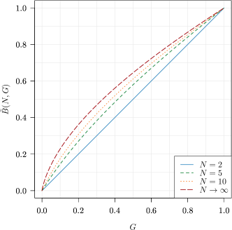
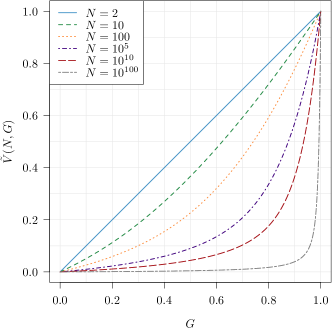
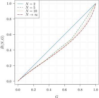
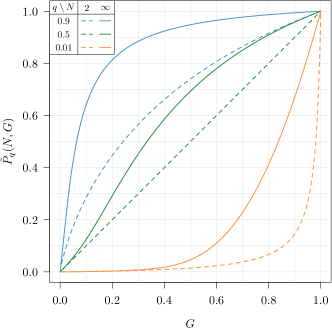
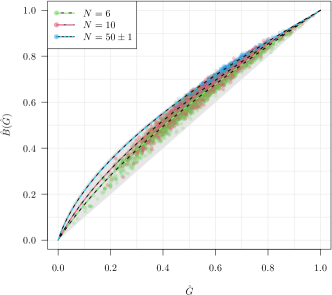
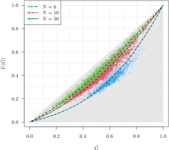
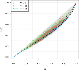
respectively (for readability, we only included the case of $G\neq 1/2$). Figure 2 depicts them for different $N$s.

Figure 2: Functional dependence between the Gini index and other inequality measures for different sample sizes $N$ in our model. The indexes are one-to-one functions of one another. Therefore, similar plots could be drawn for $V$ as a function of $B$, $H$ as a function of $P_{q}$, etc. In this context, there is no need to multiply entities without necessity. The Gini index can be used as the only measure of inequality; it is the only one that is independent of $N$.

We note that they are all strictly increasing, continuous functions of $G$. Thus, based on the derived formulas, all the indices can be expressed as one-to-one functions of one another. For instance, given some value of the Bonferroni index $B$, we can obtain the underlying $G^{*}=\tilde{B}^{-1}(N,B)$ and then compute, say, $\tilde{V}(N,G^{*})$. Even though the analytic formulae for the inverses do not exist, this still can easily be solved numerically.

In this sense, we can say that – in our model – all the aforementioned inequality indices are equivalent.

Similar derivations can be performed for many other inequality indices, although they will not necessarily enjoy analytic solutions.

4 Analysis of citation data from RePEc

Theoretical models are merely approximations of the real-world phenomena under scrutiny. Thus, empirical data might deviate from the assumed idealisations. Also, looking beyond our simple iterative process, we know that uncountably many probability vectors yield a specific Gini, Bonferroni, or any other index. After all, these measures were introduced to respond to the different needs of the practitioners; see, e.g., Imedio-Olmedo et al. (2012); McVinish and Lester (2020). Some of them are, for example, more responsive to increasing (via the principle of progressive transfers) the amount of probability mass in the tail of the distribution than others. In particular, as reported in Ciommi et al. (2022), the Gini, Bonferroni, and De Vergottini indices belong to the class of linear measures introduced in Mehran (1976). They note that for the Bonferroni and De Vergottini indices, the effect of a transfer also depends on the position of individuals, making the Bonferroni index more sensitive to transfers that occur at the lower end of the income distribution and the De Vergottini index more sensitive to variations among the richest.

Therefore, we should be interested in verifying how well our formulae describe the underlying structure of real datasets.

Let us thus consider citation data from the RePEc database (Research Papers in Economics; see https://citec.repec.org/), which features $66{,}347$ authors and $1{,}843{,}967$ papers. In the data cleansing step, we have omitted the authors who published less than $5$ cited papers and whose $h$-index was less than $3$.

This resulted in $n=36{,}425$ citation records of the form $\left(x_{1}^{(i)},\dots,x^{(i)}_{N^{(i)}}\right)$, where $N^{(i)}$ gives the total number of items published by the $i$-th author and $x_{k}^{(i)}$ gives the number of citations to their $k$-th most cited works.

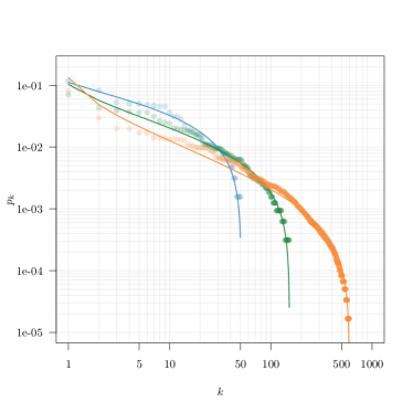
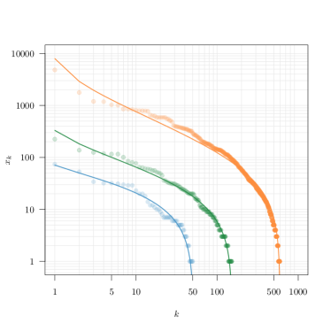
Figure 3 shows three example (quite representative of the whole database) vectors from the RePEc database: observed (points) and predicted (lines) values for $p_{k}$ (left) and their non-normalised versions, $x_{k}$ (right). We see a good fit over most parts of the data domain. This comes at no surprise, as the proposed model is equivalent to the 3DI model (Siudem et al., 2020) and we have already seen its usefulness in the case of modelling citations to computer science papers.

Figure 3: Three example citation vectors (left: normalised, right: original) and the corresponding fitted models (Eq. (1)); note the log-log scale. We note a very good fit in each case.

For each author, we compute their actual (observed) Gini index $\hat{G}^{(i)}=\mathcal{G}\left(p_{1}^{(i)},\dots,p^{(i)}_{N^{(i)}}\right)$ with $p_{k}^{(i)}=X_{k}^{(i)}/\sum_{j=1}^{N^{(i)}}X_{j}^{(i)}$.

Then, based on the derived formulae, we compute the predicted $\tilde{B}(N,\hat{G}^{(i)})$, $\tilde{V}(N,\hat{G}^{(i)})$, …, and observed $\hat{B}^{(i)}=\mathcal{B}\left(p_{1}^{(i)},\dots,p^{(i)}_{N^{(i)}}\right)$, $\hat{V}^{(i)}=\mathcal{V}\left(p_{1}^{(i)},\dots,p^{(i)}_{N^{(i)}}\right)$, …, Bonferroni, De Vergottini, and other indices.

Recall that Figure 2 describes the theoretical relationships between the Gini index and other metrics. If, overall, our model describes the real data well, we should expect to see these dependencies in the case of the RePEc vectors too.

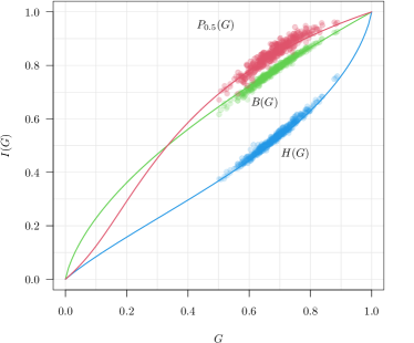
Figure 4 presents a scatter plot of the values of different indices as functions of $\hat{G}$ for all vectors with $N>200$ (the De Vergottini index was not included as it approaches $0$ for large $N$s; see Remark 2). Ideally, they should lie close to the theoretical curves (depicted as well). And this is approximately the case.

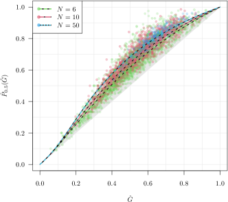
Furthermore, Figure 5 presents similar results, but for vectors of lengths $N=6$ (green), $N=10$ (pink), and $N=50\pm 1$ (blue; the $\pm 1$ part is to increase the number of data points). Additionally, we coloured the areas representing all of the possible values which could be obtained for vectors generated using our model. In other words, for any vector, we expect the pairs $(\hat{G},\hat{B})$, $(\hat{G},\hat{V})$, etc. to lie in the grey zone. This is true for the vast majority of the real data points.

The prediction errors for different vector lengths are summarised in Table 1. The error rates are usually less than 2–3%.

Overall, we observe a very good fit, confirming our theoretical derivations. The choice of the inequality measure is secondary, as the indices can be considered functions of one another. Therefore, it is best to be faithful to the simplest indicator: the Gini index.

Table 1: Left: Mean absolute prediction errors, i.e., the average of $|\hat{I}^{(i)}-\tilde{I}(N^{(i)},\hat{G}^{(i)})|$ for all vectors $\boldsymbol{p}^{(i)}$ with $N^{(i)}=N$, for $N=5,10,20,50$ and $N\geq 200$ and different indices $I$. Right: Mean prediction errors (bias), i.e., the average of $(\hat{I}^{(i)}-\tilde{I}(N^{(i)},\hat{G}^{(i)}))$. Overall, the errors are small and the longer the vector, the better the precision with which we can predict the values of the remaining indices. Note that the errors for the De Vergottini index for large $N$ are not given due to its limiting behaviour (as per Remark 2).

Mean absolute prediction errors

	$6$	$10$	$20$	$50$	$\geq 200$
$B$	0.017	0.019	0.019	0.011	0.006
$V$	0.019	0.022	0.026	0.026	—
$H$	0.027	0.026	0.022	0.017	0.011
$P_{0.5}$	0.042	0.035	0.029	0.021	0.016

       Bias $6$ $10$ $20$ $50$ $\geq 200$ $B$ -0.004 -0.013 -0.015 -0.008 -0.003 $V$ -0.001 0.002 -0.001 -0.014 — $H$ 0.021 0.02 0.018 0.014 0.011 $P_{0.5}$ 0.013 0.005 0.002 0.007 0.011

5 Analysis of income data

Additionally, let us study the Luxembourg Income Study dataset giving the family incomes in nine countries. The original data, in the form of the Lorenz (e.g., Bertoli-Barsotti and Lando, 2019) curves across the deciles ($N=10$), are given in (Bishop et al., 1991, Table 2).

Table 2 gives the prediction error for the indices studied. Overall, the errors are very small, except for the case of the $\mathcal{P}_{q}$ index with higher $q$ in Sweden, Germany, and the United Kingdom, where there is some discrepancy between the predicted and the observed Lorenz curve in their tails.

Table 2: Predicted vs observed indices for family income data (Bishop et al., 1991, Table 2); e.g., $\tilde{B}+(\hat{B}-\tilde{B})=0.50-0.01$ denotes that the predicted $\tilde{B}=0.50$ and the observed $\hat{B}=0.50-0.01$, hence the prediction error is $0.01$

country	$\hat{G}=\tilde{G}$	$\tilde{B}+(\hat{B}-\tilde{B})$	$\tilde{V}+(\hat{V}-\tilde{V})$	$\tilde{H}+(\hat{H}-\tilde{H})$	$\tilde{P}_{0.5}+(\hat{P}_{0.5}-\tilde{P}_{0.5})$	$\tilde{P}_{0.9}+(\hat{P}_{0.9}-\tilde{P}_{0.9})$
AU	$0.38$	$0.50-0.01$	$0.25+0.02$	$0.29-0.01$	$0.52-0.02$	$0.85-0.04$
CA	$0.38$	$0.50-0.01$	$0.25+0.02$	$0.28-0.01$	$0.51-0.02$	$0.84-0.02$
NL	$0.34$	$0.46-0.02$	$0.22+0.03$	$0.26-0.01$	$0.47-0.03$	$0.82-0.03$
NO	$0.34$	$0.46-0.01$	$0.22+0.02$	$0.26-0.01$	$0.46-0.02$	$0.82-0.04$
SE	$0.32$	$0.44-0.03$	$0.20+0.02$	$0.24-0.01$	$0.44-0.02$	$0.81-0.10$
CH	$0.42$	$0.54-0.02$	$0.29+0.03$	$0.31-0.02$	$0.56-0.05$	$0.87-0.01$
DE	$0.34$	$0.46-0.03$	$0.22+0.02$	$0.26-0.01$	$0.46-0.03$	$0.82-0.08$
UK	$0.38$	$0.50-0.02$	$0.25+0.02$	$0.28-0.01$	$0.51-0.02$	$0.84-0.07$
US	$0.40$	$0.52-0.01$	$0.27+0.01$	$0.30-0.01$	$0.54-0.02$	$0.86+0.00$

Figure 4: Inequality indices as functions of the Gini index for all RePEc citation vectors with $N>200$ (points). They match the derived theoretical curves (lines) very well, confirming the validity of our model, and the main hypothesis of our paper.

Figure 5: Predicted ($\tilde{B}(N,\hat{G})$ vs $\hat{G}$, $\tilde{V}(N,\hat{G})$ vs $\hat{G}$, etc.; thick curves) and observed ($\hat{B}$ vs $\hat{G}$ etc.; points) values of different inequality measures for the RePEc citation records of different lengths $N$. Our model recreates the indices with decent level of precision.

6 Conclusions

The discussed process yields $\boldsymbol{p}^{(N,G)}$ that are totally ordered by the majorisation relation $\preceq$. Following (Shorrocks and Foster, 1987) (but see also Marshall et al., 2011; Lambert, 2001; Chantreuil and Trannoy, 2011; Zheng, 2007; Bosmans, 2016), a function $I$ is an index of inequality if and only if it is symmetric and strictly Schur convex.

Hence, for all ordered probability $N$-vectors $\boldsymbol{p}\neq\boldsymbol{q}$, if $\boldsymbol{p}\preceq\boldsymbol{q}$, then $I(\boldsymbol{p})<I(\boldsymbol{q})$, where the direction of the inequality is uniquely determined by the Pigou–Dalton condition (e.g., Patty and Penn, 2019). In particular, for every vector $\boldsymbol{p}^{(N,G)}$, the parameter $G$ can be interpreted as the (normalised) Gini index $\mathcal{G}(\boldsymbol{p}^{(N,G)})=G$. This implies that $\mathcal{G}$ is an order preserving function Marshall et al. (2011) on $\{\boldsymbol{p}^{(N,G)}\}$ with respect to $G$.

In this study, we also extended this characterisation result to some other notable indices of inequality, that is, the Bonferroni, De Vergottini, Hoover and $\mathcal{P}_{q}$ indices, deriving their explicit expressions as one-to-one functions of $\mathcal{G}$. For data following closely our model, the indices can be considered equivalent. An analysis of two empirical datasets (citation vectors in economics and countrywise family incomes) confirms our results.

Acknowledgements

We are indebted to Jose Manuel Barrueco for providing us with a large snapshot of RePEc (Research Papers in Economics) data. All data are freely available at http://citec.repec.org/api.html.

This research was supported by the Australian Research Council Discovery Project ARC DP210100227 (MG).

Conflict of interest

The authors certify that they have no affiliations with or involvement in any organisation or entity with any financial interest or non-financial interest in the subject matter or materials discussed in this manuscript.

References

• Arnold (2015) Arnold, B.C., 2015. Pareto Distributions. Chapman and Hall/CRC, New York, NY, USA. doi:10.1201/b18141.
• Beliakov et al. (2016) Beliakov, G., Gagolewski, M., James, S., 2016. Penalty-based and other representations of economic inequality. International Journal of Uncertainty, Fuzziness and Knowledge-Based Systems 24(Suppl.1), 1–23. doi:10.1142/S0218488516400018.
• Bertoli-Barsotti (2023) Bertoli-Barsotti, L., 2023. Equivalent Gini coefficient, not shape parameter! Scientometrics 128, 867–870. doi:10.1007/s11192-022-04571-8.
• Bertoli-Barsotti et al. (2023) Bertoli-Barsotti, L., Gagolewski, M., Siudem, G., Żogała Siudem, B., 2023. Gini-stable Lorenz curves and their relation to the generalised Pareto distribution. Submitted for publication; see https://arxiv.org/a/gagolewski_m_1.html.
• Bertoli-Barsotti and Lando (2019) Bertoli-Barsotti, L., Lando, T., 2019. How mean rank and mean size may determine the generalised Lorenz curve: With application to citation analysis. Journal of Informetrics 13, 387–396. doi:10.1016/j.joi.2019.02.003.
• Bishop et al. (1991) Bishop, J.A., Formby, J.P., Smith, W.J., 1991. International comparisons of income inequality: Tests for Lorenz dominance across nine countries. Economica 58, 461–477.
• Bonferroni (1930) Bonferroni, C., 1930. Elementi di statistica generale. Libreria Seber, Firenze.
• Bosmans (2016) Bosmans, K., 2016. Consistent comparisons of attainment and shortfall inequality: A critical examination. Health Economics 25, 1425–1432.
• Cena et al. (2022) Cena, A., Gagolewski, M., Siudem, G., Żogała Siudem, B., 2022. Validating citation models by proxy indices. Journal of Informetrics 16, 101267. doi:10.1016/j.joi.2022.101267.
• Chantreuil and Trannoy (2011) Chantreuil, F., Trannoy, A., 2011. Inequality decomposition values. Annals of Economics and Statistics/Annales d’Économie et de Statistique 101/102, 13–36.
• Ciommi et al. (2022) Ciommi, M., Gigliarano, C., Giorgi, G., 2022. Bonferroni and de Vergottini are back: New subgroup decompositions and bipolarization measures. Fuzzy Sets and Systems 433, 22–53.
• Cowell (2000) Cowell, F.A., 2000. Measurement of inequality, in: Atkinson, A., Bourguignon, F. (Eds.), Handbook of Income Distribution. Elsevier. volume 1, pp. 87–166.
• Gagolewski et al. (2022) Gagolewski, M., Żogała Siudem, B., Siudem, G., Cena, A., 2022. Ockham’s index of citation impact. Scientometrics 127, 2829–2845. doi:10.1007/s11192-022-04345-2.
• Gini (1912) Gini, C., 1912. Variabilità e mutabilità. C. Cuppini, Bologna.
• Holme (2022) Holme, P., 2022. Universality out of order. Nature Communications 13, 2355.
• Hoover (1941) Hoover, E., 1941. Interstate redistribution of population, 1850–1940. The Journal of Economic History 1, 199–205.
• Imedio-Olmedo et al. (2012) Imedio-Olmedo, L., Parrado-Gallardo, E., Bárcena-Martín, E., 2012. Income inequality indices interpreted as measures of relative deprivation/satisfaction. Social Indicators Research 109, 471–491.
• Iñiguez et al. (2022) Iñiguez, G., Pineda, C., Gershenson, C., Barabási, A.L., 2022. Dynamics of ranking. Nature communications 13, 1646.
• Lambert (2001) Lambert, P.J., 2001. The distribution and redistribution of income (3rd Edition). Manchester University Press.
• Marshall and Olkin (2007) Marshall, A.W., Olkin, I., 2007. Life distributions: Structure of Nonparametric, Semiparametric, and Parametric Families. Springer.
• Marshall et al. (2011) Marshall, A.W., Olkin, I., Arnold, B.C., 2011. Inequalities: Theory of majorization and its applications (2nd Edition). Springer Science Business Media.
• McVinish and Lester (2020) McVinish, R., Lester, R., 2020. Measuring aggregation in parasite populations. Journal of the Royal Society Interface 17, 20190886. doi:10.1098/rsif.2019.0886.
• Mehran (1976) Mehran, F., 1976. Linear measures of income inequality. Econometrica 44, 805–809.
• Newman (2005) Newman, M., 2005. Power laws, Pareto distributions and Zipf’s law. Contemporary Physics 46, 323–351. doi:10.1080/00107510500052444.
• Patty and Penn (2019) Patty, J.W., Penn, E.M., 2019. Measuring fairness, inequality, and big data: Social choice since Arrow. Annual Review of Political Science 22, 435–460. doi:10.1146/annurev-polisci-022018-024704.
• Petersen et al. (2011) Petersen, A.M., Stanley, H.E., Succi, S., 2011. Statistical regularities in the rank-citation profile of scientists. Scientific Reports 1, 181. doi:10.1038/srep00181.
• Pickands III (1975) Pickands III, J., 1975. Statistical inference using extreme order statistics. The Annals of Statistics , 119–131.
• Price (1965) Price, D., 1965. Networks of scientific papers. Science 149, 510–515. doi:10.1126/science.149.3683.510.
• Shorrocks and Foster (1987) Shorrocks, A.F., Foster, J.E., 1987. Transfer sensitive inequality measures. The Review of Economic Studies 54, 485–497.
• Silber (2012) Silber, J., 2012. Handbook of income inequality measurement. volume 71. Springer Science & Business Media.
• Singh et al. (2022) Singh, C.K., Barme, E., Ward, R., Tupikina, L., Santolini, M., 2022. Quantifying the rise and fall of scientific fields. PLoS ONE 17, e0270131.
• Siudem et al. (2022) Siudem, G., Nowak, P., Gagolewski, M., 2022. Power laws, the Price model, and the Pareto type-2 distribution. Physica A: Statistical Mechanics and its Applications 606, 128059. doi:10.1016/j.physa.2022.128059.
• Siudem et al. (2020) Siudem, G., Żogała-Siudem, B., Cena, A., Gagolewski, M., 2020. Three dimensions of scientific impact. Proceedings of the National Academy of Sciences 117, 13896–13900. doi:10.1073/pnas.2001064117.
• Vergottini (1940) Vergottini, M.D., 1940. Sul significato di alcuni indici di concentrazione. Giornale degli Economisti e Annali di Economia 11, 317–347.
• Vergottini (1950) Vergottini, M.D., 1950. Sugli indici di concentrazione. Statistica 10, 445–454.
• Voitalov et al. (2019) Voitalov, I., van der Hoorn, P., van der Hofstad, R., Krioukov, D., 2019. Scale-free networks well done. Physical Review Research 1, 033034.
• Yitzhaki and Schechtman (2013) Yitzhaki, S., Schechtman, E., 2013. The Gini methodology: A primer on a statistical methodology. Springer.
• Zheng (2007) Zheng, B., 2007. Unit-consistent decomposable inequality measures. Economica 74, 97–111.