Efficient Convex Algorithms for Universal Kernel Learning

Abstract

The accuracy and complexity of machine learning algorithms based on kernel optimization are determined by the set of kernels over which they are able to optimize. An ideal set of kernels should: admit a linear parameterization (for tractability); be dense in the set of all kernels (for robustness); be universal (for accuracy). Recently, a framework was proposed for using positive matrices to parameterize a class of positive semi-separable kernels. Although this class can be shown to meet all three criteria, previous algorithms for optimization of such kernels were limited to classification and furthermore relied on computationally complex Semidefinite Programming (SDP) algorithms. In this paper, we pose the problem of learning semiseparable kernels as a minimax optimization problem and propose a SVD-QCQP primal-dual algorithm which dramatically reduces the computational complexity as compared with previous SDP-based approaches. Furthermore, we provide an efficient implementation of this algorithm for both classification and regression – an implementation which enables us to solve problems with 100 features and up to 30,000 datums. Finally, when applied to benchmark data, the algorithm demonstrates the potential for significant improvement in accuracy over typical (but non-convex) approaches such as Neural Nets and Random Forest with similar or better computation time.

Keywords: kernel functions, multiple kernel learning, semi-definite programming, supervised learning, universal kernels

1 Introduction

Kernel methods for classification and regression (and Support Vector Machines (SVMs) in particular) require selection of a kernel. Kernel Learning (KL) algorithms (such as those found in Xu et al., 2010; Sonnenburg et al., 2010; Yang et al., 2011) automate this task by finding the kernel, $k\in\mathcal{K}$ which optimizes an achievable metric such as the soft margin (for classification). The set of kernels, $k\in\mathcal{K}$, over which the algorithm can optimize, however, strongly influences the performance and robustness of the resulting classifier or predictor.

To understand how the choice of kernel influences performance and robustness, several properties of positive kernels have been considered. For example, a characteristic kernel was defined in Fukumizu et al. (2007) to be a kernel whose associated integral operator is injective. Alternatively, a kernel, $k$, is strictly positive definite if the associated integral operator has trivial null-space – See, e.g. Steinwart and Christmann (2008). As stated in, e.g. Steinwart (2001), it has been observed that kernels with the characteristic and strictly positive definite properties are able to perform arbitrarily well on large sets of training data. Similar to characteristic and strictly positive definite kernels, perhaps the most well-known kernel property is that of $c_{0}$-universality, which implies that the associated RKHS is dense in $\mathcal{C}$. The relationship between these and other kernel properties (using, e.g. alternative norms) has been studied extensively in, e.g. Sriperumbudur et al. (2011). In particular, the universal property implies the kernel is both characteristic and strictly positive definite, while under certain conditions the converse also holds and all three properties are equivalent (Simon-Gabriel and Schölkopf, 2018). As a result of these studies, there is a consensus that in order to be effective on large data sets, a kernel should have the universal property.

While the universal property is now well-established as being a desirable property in any kernel, much less attention has been paid to the question of what are the desirable properties of a set of kernels. This question arises when we use kernel learning algorithms to find the optimal kernel in some parameterized set. The assumption, of course, is that for any given data generating process, there is some ideal kernel whose associated feature map maximizes separability of data generated by that underlying process. Clearly, then, when constructing a set of kernels to be used in kernel learning, we would like to ensure that this set contains the ideal kernel or at least a kernel whose associated feature map closely approximates the feature map of this ideal kernel. With this in mind, (Colbert and Peet, 2020a) proposed three desirable properties of a set of kernels $\mathcal{K}$ - tractability, density, and universality. Specifically, $\mathcal{K}$ is said to be tractable if $\mathcal{K}$ is convex (or, preferably, a linear variety) - implying the kernel learning problem is solvable in polynomial time (e.g. Rakotomamonjy et al., 2008; Jain et al., 2012; Lanckriet et al., 2004; Qiu and Lane, 2005). The set $\mathcal{K}$ has the density property if, for any $\epsilon>0$ and any positive kernel, $k^{*}$ there exists a $k\in\mathcal{K}$ where $\lVert{k-k^{*}}\rVert\leq\epsilon$. The density property implies that kernels from this set can approximate the feature map of the ideal kernel arbitrarily well ( which then implies the resulting learned kernel will perform well on untrained data). Finally, the set $\mathcal{K}$ is said to have the universal property if any $k\in\mathcal{K}$ is universal.

Having defined desirably properties in a set of kernels, the question becomes how to parameterize such a set. While there are many ways of parameterizing sets of kernels (See Gönen and Alpaydın, 2011, for a survey), not all such parameterizations result in a convex kernel learning algorithm. Furthermore, at present, there is no tractable parameterization which is dense in the set of all possible kernels. To address this problem, in Colbert and Peet (2020a), a general framework was proposed for using positive matrices and bases to parameterize families of positive kernels (as opposed to positive kernel matrices as in Lanckriet et al., 2004; Qiu and Lane, 2005; Ni et al., 2006). This framework allows one to define a basis of kernels for a class of integral operators and then to use SDP to find kernels which represent squares of such operators – implying that the resulting kernels define positive operators. In particular, Colbert and Peet (2020a) proposed a set of basis functions which were then used to parameterize positive integral operators of the form (using one-dimension for simplicity)

$$(\mathcal{P}\mathbf{x})(s):=k_{1a}(s)\int_{0}^{s}k_{1b}(\theta)\mathbf{x}(\theta)d\theta+k_{2a}(s)\int_{s}^{1}k_{2b}(\theta)\mathbf{x}(\theta)d\theta,$$ (1)

which correspond to what are known (in one-dimension) as semiseparable kernels – See, e.g. Gohberg et al. (2012). In $n$-dimensions, a kernel constructed using this particular parameterization was referred to as a Tessellated Kernel (TK) – indicative of their blockwise partition of the domain (a feature resulting from the semi-separable structure and reminiscent of the activation functions used in neural nets). It was further shown that the interior of this class of kernels was universal and the set of such kernels was dense in the set of all positive kernels. Using this positive matrix parameterization of the family of Tessellated Kernels, it was shown in Colbert and Peet (2020a) that the associated SVM kernel learning algorithm could be posed as an SDP and that the solution to this SDP achieves superior Test Set Accuracy (TSA) when compared with a representative sample of existing classification algorithms (including non-convex kernel learning methods such as simple Neural Nets).

Unfortunately, however, although the TSA data reported in Colbert and Peet (2020a) showed improvement over existing classification algorithms, this accuracy came at the cost of significant increases in computational complexity – a factor attributable to the high complexity of primal-dual interior point algorithms for solving SDP. Unlike Quadratic Programming (QP), which is used to solve the underlying SVM or Support Vector Regression (SVR) problem for a fixed kernel, the use of SDP, Quadratically Constrained Quadratic Programming (QCQP) and Second Order Cone Programming (SOCP) for kernel learning significantly limits the amount of training data which can be processed. Note that while this complexity issue has been partially addressed in the context of MKL (which considered an efficient reduction to QP complexity in Jain et al., 2012), such a reduction to QP has not previously been proposed for SDP-based algorithms such as kernel matrix learning. The goal of this paper, then, is to propose an algorithm for optimizing over families of kernels parameterized by positive matrices, but without the use of SDP and its associated computational overhead.

To achieve this goal, we show that the problem of kernel learning using a family of kernels parameterized by positive matrices can be equivalently posed as a saddle-point problem. Specifically, we decompose the problem into primal and dual sub-problems, $OPT\_A$ and $OPT\_P$ - similar to the approach taken in Rakotomamonjy et al. (2008) and Jain et al. (2012). Next, we show that $OPT\_P$ admits an analytic solution using the Singular Value Decomposition (SVD) - implying a worst-case computational complexity of $O(n_{P}^{3})$ where $n_{P}^{2}/2+n_{P}$ is the number of parameters in the family of kernels. In addition, $OPT\_A$ is a convex QP and may be similarly solved with a complexity of $O(m^{3})$, where $m$ is the number of data points. These sub-problems are combined using a two-step Franke-Wolfe type algorithm and we show that termination at $OPT\_A=OPT\_P$ is equivalent to global optimality. This compares favorably with the theoretical complexity (Brian and Young, 2007) of the SDP implementation of $O(m_{s}n_{s}^{3}+m_{s}^{2}n_{s}^{2})$, where $n_{s}=n_{P}+m$ and $m_{s}=n_{P}^{2}+2m$ – yielding approximately $O(m^{4})$ with respect to $m$ and $O(n_{P}^{6})$ with respect to $n_{P}$.

The resulting algorithm, then, does not require the use of SDP, QCQP or SOCP and, when applied to several standard test cases, has observed complexity which scales as $O(m^{2.3})$ or less. Furthermore, while the proven convergence rate of the proposed Franke-Wolfe type algorithm is linear, we propose a secondary implementation which results in a provable quadratic convergence rate. Note that, in practice, when applied to typical data sets, we find that the Franke-Wolfe type algorithm initially outperforms the secondary quadratically convergent algorithm. As a result, our final algorithm combines both approaches, where the quadratically convergent algorithm is only used when highly accurate solutions are required.

In addition to the proposed algorithm, this paper also extends the convex kernel learning framework proposed in Colbert and Peet (2020a) to the problem of kernel learning for regression. The kernel learning problem in regression has been studied for kernel matrix learning as in Lanckriet et al. (2004) and for MKL in e.g. Rakotomamonjy et al. (2008); Jain et al. (2012). However, the regression problem has not previously been considered using the generalized framework for kernel learning presented in Colbert and Peet (2020a). In this paper, we provide such extension and demonstrate significant increases in performance, as measured by both computation time and Mean Square Error (MSE) when compared to other optimization-based kernel learning algorithms as well as when compared to more heuristic approaches such as Random Forest and deep learning.

2 Notation

We use $\mathbb{N},\mathbb{R}$ to denote the natural and real numbers, respectively. We use $\mathbf{1}^{n}\in\mathbb{R}^{n}$ to denoted the vector of ones. For $x\in\mathbb{R}^{n}$ we use $\|x\|_{p}$ for the $L_{p}$-norm and use $x\geq 0$ to indicate the positive orthant – i.e. $x_{i}\geq 0$ for all $i$. For $x,y\in\mathbb{R}^{n}$, $x\odot y$ denotes elementwise multiplication. The space of $n\times n$-square real symmetric matrices is denoted $\mathbb{S}^{n}$ with $\mathbb{S}^{n}_{+}\subset\mathbb{S}^{n}$ being the cone of positive definite matrices. For $A,B\in\mathbb{R}^{n\times n}$, $\langle A,B\rangle$ denotes the Frobenius matrix inner product. For a compact set $X\subset\mathbb{R}^{n}$, we denote $\mathcal{C}(X)$ to be the space of scalar continuous functions defined on $X$ and equipped with the uniform norm $\|f\|_{\mathcal{C}}:=\sup_{x\in X}|f(x)|$. For a given positive definite kernel $k\in\mathcal{C}(X\times X)$, ${\mathcal{H}}_{k}$ denotes the associated Reproducing Kernel Hilbert Space (RKHS), where the subscript $k$ is dropped if clear from context.

3 Kernel Sets and Kernel learning

Consider a generalized representation of the kernel learning problem, which encompasses both classification and regression where (using the representor theorem as in Schölkopf et al., 2001) the learned function is of the form $f_{\alpha,k}(z)=\sum_{i=1}^{m}\alpha_{i}k(x_{i},z)$.

$$\min_{k\in\mathcal{K}}\min_{\alpha\in\mathbb{R}^{m},b}\lVert{f_{\alpha,k}}\rVert^{2}+C\sum\nolimits_{i=1}^{m}l(f_{\alpha,k},b)_{y_{i},x_{i}}.$$ (2)

Here $\lVert{f_{\alpha,k}}\rVert=\sum_{i=1}^{m}\sum_{j=1}^{m}\alpha_{i}\alpha_{j}k(x_{i},x_{j})$ is the norm in the Reproducing Kernel Hilbert Space (RKHS) and $l(f_{\alpha,k},b)_{y_{i},x_{i}}$ is the loss function defined for SVM binary classification and SVM regression as $l_{c}(f_{\alpha,k},b)_{y_{i},x_{i}}$ and $l_{r}(f_{\alpha,k},b)_{y_{i},x_{i}}$, respectively, where

$$l_{c}(f_{\alpha,k},b)_{y_{i},x_{i}} =\max\{0,1-y_{i}(f_{\alpha,k}(x_{i})-b)\},$$

$$l_{r}(f_{\alpha,k},b)_{y_{i},x_{i}} =\max\{0,|y_{i}-(f_{\alpha,k}(x_{i})-b)|-\epsilon\}.$$

The properties of the classifier/predictor, $f_{\alpha,k}$, resulting from Optimization Problem 2 will depend on the properties of the set $\mathcal{K}$, which is presumed to be a subset of the convex cone of all positive kernels. To understand how the choice of $\mathcal{K}$ influences the tractability of the optimization problem and the resulting fit, we consider three properties of the set, $\mathcal{K}$. These properties can be precisely defined as follows.

3.1 Tractability

We say a set of kernel functions, $\mathcal{K}$, is tractable if it can be represented using a countable basis.

Definition 1

The set of kernels $\mathcal{K}$ is tractable if there exist a countable set $\{G_{i}(x,y)\}_{i=1}^{\infty}$ such that, for any $k\in\mathcal{K}$, there exists $n_{k}\in\mathbb{N}$ where $k(x,y)=\sum_{i=1}^{n_{k}}v_{i}G_{i}(x,y)$ for some $v\in\mathbb{R}^{n_{k}}$.

Note the $G_{i}(x,y)$ need not be positive kernel functions. The tractable property is required for the associated kernel learning problem to be solvable in polynomial time.

3.2 Universality

Universal kernel functions always have positive definite (full rank) kernel matrices, implying that for arbitrary data $\{y_{i},x_{i}\}_{i=1}^{m}$, there exists a function $f(z)=\sum_{i=1}^{m}\alpha_{i}k(x_{i},z)$, such that $f(x_{j})=y_{j}$ for all $j=1,..,m$. Conversely, if a kernel is not universal, then there exists a data set $\{x_{i},y_{i}\}_{i=1}^{m}$ such that for any $\alpha\in\mathbb{R}^{m}$, there exists some $j\in\{1,\cdots,m\}$ such that $f(y_{j})\neq\sum_{i=1}^{m}\alpha_{i}k(x_{i},x_{j})$. The universality property ensures that the classifier of an SVM designed using a universal kernel will become increasingly precise as the training data increases, whereas classifiers from a non-universal kernel have limited ability to fit data sets. (See Micchelli et al., 2006).

Definition 2 (Schölkopf et al. (2001))

A kernel $k:X\times X\rightarrow\mathbb{R}$ is said to be universal on the compact metric space $X$ if it is continuous and there exists an inner-product space $\mathcal{W}$ and feature map, $\Phi:X\rightarrow\mathcal{W}$ such that $k(x,y)=\langle\Phi(x),\Phi(y)\rangle_{\mathcal{W}}$ and where the unique Reproducing Kernel Hilbert Space (RKHS), $\mathcal{H}:=\{f\;:\;f(x)=\langle v,\Phi(x)\rangle,\;v\in\mathcal{W}\}$ with associated norm $\lVert{f}\rVert_{\mathcal{H}}:=\inf_{v}\{\lVert{v}\rVert_{\mathcal{W}}\;:\;f(x)=\langle v,\Phi(x)\rangle\}$ is dense in $\mathcal{C}(X):=\{f\,:\,X\rightarrow\mathbb{R}\;:\;$f$\,\text{ is continuous}\}$ where $\lVert{f}\rVert_{\mathcal{C}}:=\sup_{x\in X}|f(x)|$.

Recall that the universality property implies the strictly positive definite and characteristic properties on compact domains. The following definition extends the universal property to a set of kernels.

Definition 3

A set of kernel functions $\mathcal{K}$ has the universal property if every kernel function $k\in\mathcal{K}$ is universal.

3.3 Density

The third property of a kernel set, $\mathcal{K}$, is density which ensures that a kernel can be chosen from $\mathcal{K}$ with an associated feature map which optimizes fitting of the data in the associated feature space. This optimality of fit in the feature space may be interpreted differently for SVM and SVR. Specifically, considering SVM for classification, the kernel learning problem determines the kernel $k\in\mathcal{K}$ for which we may obtain the maximum separation in the kernel-associated feature space. According to Boehmke and Greenwell (2019), increasing this separation distance makes the resulting classifier more robust (generalizable). The density property, then, ensures that the resulting kernel learning algorithm will be maximally robust (generalizable) in the sense of separation distance. In the case of SVR, meanwhile, the kernel learning problem finds the kernel $k\in\mathcal{K}$ which permits the “flattest” (see Smola and Schölkopf, 2004) function in feature space. In this case, the density property ensures that the resulting kernel learning algorithm will be maximally robust (generalizable) in the sense of flatness.

Note that the density properties is distinct from the universality property. For instance consider a set containing a single Gaussian kernel function - which is clearly not ideal for kernel learning. The set containing a single Gaussian is tractable (it has only one element) and every member of the set is universal. However, it is not dense.

These arguments motivate the following definition of the pointwise density property.

Definition 4

The set of kernels $\mathcal{K}$ is said to be pointwise dense if for any positive kernel, $k^{*}$, any set of data $\{x_{i}\}_{i=1}^{m}$, and any $\epsilon>0$, there exists $k\in\mathcal{K}$ such that

$$\lVert{k(x_{i},x_{j})-k^{*}(x_{i},x_{j})}\rVert\leq\epsilon.$$

4 A General Framework for Representation of Tractable Kernel Sets

Having defined three desirable properties of a set of kernels, we now consider a framework designed to facilitate the creation of sets of kernels which meet these criteria. This framework ensures tractability by providing a linear map from positive matrices to positive kernels. This map is defined by a set of bases, $N$. These bases themselves parameterize kernels the image of whose associated integral operators define the feature space. As we will show in Section 5, kernel learning over a set of kernels parameterized in this way can be performed efficiently using a combination of QP and the SVD. Moreover, as we will show in Section 6, suitable choices of $N$ will ensure that the set of kernels has the density and universality properties.

Lemma 5

Let $N$ be any bounded measurable function $N:Y\times X\rightarrow\mathbb{R}^{n_{P}}$ on compact $X$ and $Y$. If we define

$${\mathcal{K}}:=\left\{k~{}|~{}k(x,y)=\int_{Y}N(z,x)^{T}PN(z,y)dz,\quad P\geq 0\right\},$$ (3)

then any $k\in\mathcal{K}$ is a positive kernel function and $\mathcal{K}$ is tractable.

Proof  The proof is straightforward. Given a kernel, $k$, denote the associated integral operator by $I_{k}$ so that

$$(I_{k}\phi)(s)=\int_{X}k(s,t)\phi(t)dt.$$

If $k\in\mathcal{K}$, it has the form of Eqn. (3) for some $P\geq 0$. Now define $k_{\frac{1}{2}}(x,y):=P^{\frac{1}{2}}N(x,y)$. Then $I_{k}=I_{k_{\frac{1}{2}}}^{*}I_{k_{\frac{1}{2}}}\geq 0$ where adjoint is defined with respect to the $L_{2}$ inner product. This establishes positivity of the kernel. Note that if $I_{k_{\frac{1}{2}}}\in\mathcal{A}$ for some *-algebra $\mathcal{A}$, then $I_{k}\in\mathcal{A}$.

For tractability, we note that for a given $N$, the map $P\mapsto k$ is linear. Specifically,

$$k(x,y)=\sum\nolimits_{i,j=1}^{n_{P}}P_{i,j}G_{i,j}(x,y),$$

where

$$G_{i,j}(x,y)=\int_{Y}N_{i}(z,x)N_{j}(z,y)dz,$$ (4)

and thus by Definition 1, $\mathcal{K}$ is tractable.  

Note:

Using the notation for integral operators in the proof of Lemma 5, we also note that for any $k\in\mathcal{K}$,

$$I_{k}=\sum\nolimits_{i,j=1}^{n_{P}}P_{i,j}I_{G_{i,j}}=\sum\nolimits_{i,j=1}^{n_{P}}P_{i,j}I_{N_{i}}^{*}I_{N_{j}}.$$ (5)

For convenience, we refer to a set of kernels defined as in Eqn. (3) as a Generalized Kernel Set, a kernel from such set as a Generalized Kernel, and the associated kernel learning problem in (2) as Generalized Kernel Learning (GKL) (3). This is to distinguish such kernels, sets and problems from Tessellated Kernel Learning, which arises from a particular choice of $N$ in the parameterization of $\mathcal{K}$. This distinction is significant, as the algorithms in Sections 5 apply to the Generalized Kernel Learning problem, while the results in Section 6 only apply to the particular case of Tessellated Kernel Learning.

5 An Efficient Algorithm for Generalized Kernel Learning in Classification and Regression Problems

In this section, we assume a family of kernel functions, $\mathcal{K}$, has been parameterized as in (3), and formulate the kernel learning optimization problem for both classification and regression — representing this as a minimax saddle point problem. This formulation enables a decomposition into convex primal and dual sub-problems, $OPT\_A(P)$ and $OPT\_P(\alpha)$ with no duality gap. We then consider the Frank-Wolfe algorithm and show using Danskin’s Theorem that the gradient step can be efficiently computed using the primal and dual sub-problems. Finally, we propose efficient algorithms for computing $OPT\_A(P)$ and $OPT\_P(\alpha)$: in the former case using an efficient Sequential Minimal Optimization (SMO) algorithm for convex QP and in the latter case, using an analytic solution based on the SVD.

5.1 Primal-Dual Decomposition

For convenience, we define the feasible sets for the sub-problems as

$$\mathcal{X}: =\{P\in\mathbb{S}^{n_{P}}\;:\;\text{trace}(P)=n_{P},\;P>0\},$$

$$\mathcal{Y}_{c}: =\{\alpha\in\mathbb{R}^{m}\;:\;\sum\nolimits_{i=1}^{m}\alpha_{i}y_{i}=0,\;0\leq\alpha_{i}\leq C\},$$

$$\mathcal{Y}_{r}: =\{\alpha\in\mathbb{R}^{m}\;:\;\sum\nolimits_{i=1}^{m}\alpha_{i}=0,\;\alpha_{i}\in[-C,C]\},$$

where $m$ and $C$ are as defined in Optimization Problem 2. In this section, we typically use the generic form $\mathcal{Y}_{\star}$ to refer to either $\mathcal{Y}_{c}$ or $\mathcal{Y}_{r}$ depending on whether the algorithm is being applied to the classification or regression problem. To specify the objective function we define $\lambda(\alpha,P)$ as

$$\lambda(\alpha,P):=-\frac{1}{2}\sum\limits_{i=1}^{m}\sum\limits_{j=1}^{m}\alpha_{i}\alpha_{j}\int_{Y}N(z,x_{i})^{T}PN(z,y_{j})dz,$$ (6)

where the bases, $N$, and domain, $Y$, are those used to specify the kernel set, $\mathcal{K}$, in Eqn. (3). Additionally, we define $\kappa_{c}(\alpha):=\sum\nolimits_{i=1}^{m}\alpha_{i}$ and

$$\kappa_{r}(\alpha):=-\epsilon\sum\nolimits_{i=1}^{m}|\alpha_{i}|+\sum\nolimits_{i=1}^{m}y_{i}\alpha_{i}$$

where, again, we use $\kappa_{\star}=\kappa_{c}$ for classification and $\kappa_{\star}=\kappa_{r}$ for regression.

Using the formulation in, e.g. Lanckriet et al. (2004), it can be shown that if the family $\mathcal{K}$ is parameterized as in Eqn. (3), then the Generalized Kernel Learning optimization problem in Eqn. (2) can be recast as the following minimax saddle point optimization problem.

$$OPT_{P} :=\min_{P\in\mathcal{X}}\max_{~{}\alpha\in\mathcal{Y}_{\star}}\quad\lambda(e_{\star}\odot\alpha,P)+\kappa_{\star}(\alpha),$$ (7)

where $\odot$ indicates elementwise multiplication. For classification, $\mathcal{Y}_{\star}=\mathcal{Y}_{c}$, $\kappa_{\star}=\kappa_{c}$, and $e_{\star}=e_{c}:=y$ (vector of labels). For regression, $\mathcal{Y}_{\star}=\mathcal{Y}_{c}$, $\kappa_{\star}=\kappa_{r}$, and $e_{\star}=e_{r}:=\mathbf{1}_{m}$ (vector of ones).

Minimax Duality To find the dual, $OPT_{D}$ of the kernel learning optimization problem ($OPT_{P}$), we formulate two sub-problems:

$$OPT\_A(P)~{}:=\max_{\alpha\in\mathcal{Y}_{\star}}\lambda(e_{\star}\odot\alpha,P)+\kappa_{\star}(\alpha)$$ (8)

and

$$OPT\_{P}(\alpha):=\min_{P\in\mathcal{X}}~{}~{}\lambda(e_{\star}\odot\alpha,P)+\kappa_{\star}(\alpha).$$ (9)

Now, we have that

$$OPT_{P}=\min_{P\in\mathcal{X}}~{}OPT\_A(P)$$

and its minmax dual is

$$OPT_{D} =\max_{\alpha\in\mathcal{Y}_{\star}}OPT\_P(\alpha)=\max_{~{}\alpha\in\mathcal{Y}_{\star}}\min_{P\in\mathcal{X}}\quad\lambda(e_{\star}\odot\alpha,P)+\kappa_{\star}(\alpha).$$

The following lemma states that there is no duality gap between $OPT_{P}$ and $OPT_{D}$ - a property we will use in our termination criterion.

Lemma 6

$OPT_{P}=OPT_{D}$. Furthermore, $\{\alpha^{*},P^{*}\}$ solve $OPT_{P}$ if and only if $OPT\_P(\alpha^{*})=OPT\_A(P^{*})$.

Proof 

For any minmax optimization problem with objective function $\phi$, we have

$$d^{*}=\max_{\alpha\in\mathcal{Y}}\min_{P\in\mathcal{X}}\phi(P,\alpha)\leq\min_{P\in\mathcal{X}}\max_{\alpha\in\mathcal{Y}}\phi(P,\alpha)=p^{*}$$

and strong duality holds ($p^{*}-d^{*}=0$) if $\mathcal{X}$ and $\mathcal{Y}$ are both convex and one is compact, $\phi(\cdot,\alpha)$ is convex for every $\alpha\in\mathcal{Y}$ and $\phi(P,\cdot)$ is concave for every $P\in\mathcal{X}$, and the function $\phi$ is continuous (See Fan, 1953). In our case, these conditions hold for both classification ($\phi(P,\alpha)=\lambda(\alpha\odot y,P)+\kappa_{c}(\alpha)$) and regression ($\phi(P,\alpha)=\lambda(\alpha,P)+\kappa_{r}(\alpha))$. Hence $OPT_{P}=OPT_{D}$. Furthermore, if $\{\alpha^{*},P^{*}\}$ solve $OPT_{P}$ then

$$OPT\_P(\alpha^{*}) =\max_{\alpha\in\mathcal{Y}}OPT\_P(\alpha)=\min_{P\in\mathcal{X}}OPT\_A(P)=OPT\_A(P^{*}).$$

Conversely, suppose $\alpha\in\mathcal{Y}$, $P\in\mathcal{X}$, then

$$\small OPT\_P(\alpha)\leq\max_{\alpha\in\mathcal{Y}}\;OPT\_P(\alpha) =OPT\_P(\alpha^{*})$$

$$=OPT\_A(P^{*})=\min_{P\in\mathcal{X}}OPT\_A(P)\leq OPT\_A(P).$$

Hence if $OPT\_A(P)=OPT\_P(\alpha)$, then $OPT\_A(P)=OPT\_A(P^{*})=OPT\_P(\alpha^{*})=OPT\_P(\alpha)$ and hence $P$ and $\alpha$ solve $OPT\_A$ and $OPT\_P$, respectively.  
Finally, we show that $OPT\_A(P)$ is convex with respect to $P$ - a property we will use in Thm. 17.

Lemma 7

Let $OPT\_A(P)$ be as defined in (8). Then, the function $OPT\_A(P)$ is convex with respect to $P$.

Proof 

For simplicity, let $e_{\star}=e_{r}\in\mathbb{R}^{m}$ which is the vector of ones and hence $e_{\star}\odot\alpha=\alpha$. The function $OPT\_A(P):\mathcal{X}\rightarrow\mathbb{R}$ is convex if and only if for any $X,V\in\mathcal{X}$, $g(t):=OPT\_A(X+tV)$ is convex in $t$ for all $t\in H:=\{s\in\mathbb{R}\,|\,X+sV\succeq 0\}$. To prove convexity of $g(t)$ we must prove that,

$$g(\theta t_{1}+(1-\theta)t_{2})\leq\theta g(t_{1})+(1-\theta)g(t_{2})$$

for any $\theta\in[0,1]$ and $t_{1},t_{2}\in H$. Since $t_{1},t_{2}\in H$, by definition if we let $P_{1}=X+t_{1}V$ and $P_{2}=X+t_{2}V$, then $P_{1},P_{2}$ are positive semi-definite matrices. Now, since $\lambda(\alpha,P)$ is linear with respect to $P$ we have that,

$$g(\theta t_{1}+(1-\theta)t_{2}) =\max_{\alpha\in\mathcal{Y}_{\star}}\lambda(\alpha,X+(\theta t_{1}+(1-\theta)t_{2})V)+\kappa_{\star}(\alpha)$$

$$=\max_{~{}\alpha\in\mathcal{Y}_{\star}}\lambda(\alpha,\theta P_{1}+(1-\theta)P_{2})+\kappa_{\star}(\alpha)$$

$$=\max_{~{}\alpha\in\mathcal{Y}_{\star}}\theta\left(\lambda(\alpha,P_{1})+\kappa_{\star}(\alpha)\right)+(1-\theta)\left(\lambda(\alpha,P_{2})+\kappa_{\star}(\alpha)\right)$$

$$\leq\max_{~{}\alpha\in\mathcal{Y}_{\star}}\theta\left(\lambda(\alpha,P_{1})+\kappa_{\star}(\alpha)\right)+\max_{~{}\alpha\in\mathcal{Y}_{\star}}(1-\theta)\left(\lambda(\alpha,P_{2})+\kappa_{\star}(\alpha)\right)$$

$$\leq\theta g(t_{1})+(1-\theta)g(t_{2}).$$

The proof similarly holds for $e_{\star}=e_{c}$.  

  Initialize $P_{0}$ as any point in $\mathcal{X}$.;

  Step 1:

     $S_{k}=\arg\min_{S\in\mathcal{X}}\left<\nabla_{Q}f(Q)|_{Q=P_{k}},S\right>$

  Step 2:

     $\displaystyle\gamma_{k}=\arg\min_{\begin{subarray}{c}\gamma\in[0,1]\end{subarray}}f(P_{k}+\gamma(S_{k}-P_{k}))$

  Step 3:

     $P_{k+1}=P_{k}+\gamma_{k}\left(S_{k}-P_{k}\right),k=k+1,$

  Return to step 1 unless stopping criteria is met.

Algorithm 1 The Frank-Wolfe Algorithm for Matrices.

  Initialize $P_{0}=I$, $k=0$, $\alpha_{0}=OPT\_A(P_{0})$;

  Step 1a:   $\alpha_{k}=\arg OPT\_A(P_{k})$

  Step 1b:   $S_{k}=\arg OPT\_P(\alpha_{k})$

  Step 2:

     $\displaystyle\gamma_{k}=\arg\min_{\begin{subarray}{c}\gamma\in[0,1]\end{subarray}}OPT\_A(P_{k}+\gamma(S_{k}-P_{k}))$

  Step 3:

     $P_{k+1}=P_{k}+\gamma_{k}(S_{k}-P_{k})$, $k=k+1$

  Return to step 1 unless $OPT\_P(\alpha_{k})-OPT\_A(P_{k})<\epsilon.$

Algorithm 2 Proposed FW Algorithm for GKL.

5.2 Primal-Dual Frank-Wolfe Algorithm

For an optimization problem of the form

$$\min_{S\in\mathcal{X}}f(S),$$

where $\mathcal{X}$ is a convex subset of matrices and $\left<\cdot,\cdot\right>$ is the Frobenius matrix inner product, the Frank-Wolfe (FW) algorithm (See, e.g. Frank and Wolfe, 1956) may be defined as in Algorithm 1.

In our case, we have $f(Q)=OPT\_A(Q)$ so that

$$OPT_{P}=\min_{P\in\mathcal{X}}OPT\_A(P).$$

Unfortunately, implementation of the FW algorithm requires us to compute $\nabla_{Q}OPT\_A(Q)|_{Q=P_{k}}$ at each iteration. Fortunately, as shown in Subsections 5.3 and 5.4, we may efficiently compute the sub-problems $OPT\_A$ and $OPT\_P$. Furthermore, in Theorem 9, we will show that these sub-problems can be used to efficiently compute the gradient $\nabla_{Q}OPT\_A(Q)|_{Q=P_{k}}$ - allowing for an efficient implementation of the FW algorithm. Theorem 9 uses Danskin’s theorem proposed in Bertsekas (2016) as stated below.

Proposition 8 (Danskin’s Theorem (Bertsekas, 2016))

Let ${\mathcal{Y}\subset\mathbb{R}^{m}}$ be a compact set, and let $\phi:\mathcal{X}\times\mathcal{Y}\rightarrow\mathbb{R}$ be continuous such that $\phi(\cdot,\alpha):\mathcal{X}\rightarrow\mathbb{R}$ is convex for each $\alpha\in\mathcal{Y}$. Then if

$${\mathcal{Y}_{0}}(P)=\left\{\bar{\alpha}~{}~{}|~{}~{}\phi(P,\bar{\alpha})=\max_{\alpha\in{\mathcal{Y}}}\phi(P,\alpha)\right\}$$

consists of only one unique point, $\bar{\alpha}$, and $\phi(\cdot,\bar{\alpha})$ is differentiable at $P$ then $f(P)=\max_{\alpha\in\mathcal{Y}}\phi(P,\alpha)$ is differentiable at $P$ and

$$\nabla_{P}f(P)=\nabla_{P}\phi(P,\bar{\alpha}),$$

where $\nabla_{P}\phi(P,\bar{\alpha})$ is the vector with coordinates

$$\frac{\partial\phi(P,\bar{\alpha})}{\partial P_{i}},\quad i=1,...,n.$$

Lemma 9

If $OPT\_A$ and $OPT\_P$ are as defined in Eqns. (8) and (9), then for any $P_{k}\geq 0$, we have

$$\arg\min_{S\in\mathcal{X}}\left<\nabla_{Q}OPT\_A(Q)|_{Q=P_{k}},S\right>=\arg OPT\_P(\arg OPT\_A(P_{k})).$$

Proof  For simplicity, we utilize the definition of $D(\alpha)$ which will be given in Eqn. (10) so that $\lambda(e_{\star}\odot\alpha,P):=\left<D(\alpha),P\right>$. Now, since $\lambda(\alpha,P)$ is strictly convex in $\alpha$, for any $P_{k}>0$, $OPT\_A(P_{k})$ has a unique solution and hence we have by Danskin’s Theorem that

$$\arg\min_{S\in\mathcal{X}}{\big{<}}\nabla_{Q}OPT\_A(Q)|_{Q=P_{k}},S{\big{>}}$$

$$=\arg\min_{S\in\mathcal{X}}{\big{<}}\nabla_{Q}\left[\max_{\alpha\in\mathcal{Y}_{\star}}\left(\left<D(\alpha),Q\right>+\kappa_{\star}(\alpha)\right)\right]_{Q=P_{k}},S{\big{>}}$$

$$=\arg\min_{S\in\mathcal{X}}{\big{<}}\nabla_{Q}\left[\left<D(\bar{\alpha}),Q\right>+\kappa_{\star}(\bar{\alpha})\right]_{Q=P_{k}},S{\big{>}}$$

where $\bar{\alpha}=\arg OPT\_A(P_{k})$. Hence,

$$\arg\min_{S\in\mathcal{X}}{\big{<}}\nabla_{Q}\left[\left<D(\bar{\alpha}),Q\right>+\kappa_{\star}(\bar{\alpha})\right]_{Q=P_{k}},S{\big{>}}=\arg\min_{S\in\mathcal{X}}{\big{<}}\nabla_{Q}\left[\left<D(\bar{\alpha}),Q\right>\right]_{Q=P_{k}},S{\big{>}}$$

$$=\arg\min_{S\in\mathcal{X}}{\big{<}}D(\bar{\alpha}),S{\big{>}}=\arg OPT\_P(\bar{\alpha})=\arg OPT\_P(\arg OPT\_A(P_{k})).$$

 

We now propose an efficient implementation of the FW GKL algorithm, as defined in Algorithm 2, based on efficient algorithms for computing $OPT\_A$ and $OPT\_P$ as will be defined in Subsections 5.3 and 5.4.

In the following theorem, we use convergence properties of the FW GKL algorithm to show that Algorithm 2 has worst-case linear convergence. Note that when higher accuracy is required, we may utilize recently proposed primal-dual algorithms for quadratic convergence, as will be discussed in Section 5.5.

Theorem 10

Algorithm 2 returns iterates $P_{k}$ and $\alpha_{k}$ such that, $|\lambda(\alpha_{k},P_{k})+\kappa_{\star}(\alpha_{k})-OPT_{P}|<O(\frac{1}{k})$.

Proof  If we define $f=OPT\_A$, then Theorem 9 shows that $f$ is differentiable and, if the $P_{k}$ satisfy Algorithm 2, that the $P_{k}$ also satisfy Algorithm 1. In addition, Lemma 7 shows that $f(Q)=OPT\_A(Q)$ is convex in $Q$. It has been shown in, e.g. Jaggi (2013), that if $\mathcal{X}$ is convex and compact and $f(Q)$ is convex and differentiable on $Q\in\mathcal{X}$, then the FW Algorithm produces iterates $P_{k}$, such that, $f(P_{k})-f(P^{*})<O(\frac{1}{k})$ where

$$f(P^{*})=\min_{P\in\mathcal{X}}f(P)=\min_{P\in\mathcal{X}}OPT\_A(P)=OPT_{P}.$$

Finally, we note that

$$\lambda(\alpha_{k},P_{k})+\kappa_{\star}(\alpha_{k})= \lambda(\arg OPT\_A(P_{k}),P_{k})+\kappa_{\star}(\arg OPT\_A(P_{k}))$$

$$=\max_{\alpha\in\mathcal{Y}_{\star}}\lambda(\alpha,P_{k})+\kappa_{\star}(\alpha)=OPT\_A(P_{k})=f(P_{k}),$$

which completes the proof.  
In the following subsections, we provide efficient algorithms for computing the sub-problems $OPT\_A$ and $OPT\_P$.

5.3 Step 1, Part A: Solving $OPT\_A(P)$

For a given $P>0$, $OPT\_A(P)$ is a convex Quadratic Program (QP). General purpose QP solvers have a worst-case complexity which scales as $O(m^{3})$ (See Ye and Tse (1989)) where, when applied to $OPT\_A$, $m$ becomes the number of samples. This computational complexity may be improved, however, by noting that $OPT\_A$ is compatible with the representation defined in Chang and Lin (2011) for QPs derived from support vector machine problems. In this case, the algorithm in LibSVM reduces the computational burden somewhat. This improved performance is illustrated in Figure 2 where we observe the achieved complexity scales as $O(m^{2.3})$. Note that for the 2-step algorithm proposed in this manuscript, solving the QP in $OPT\_A(P)$ is significantly slower that solving the Singular Value Decomposition (SVD) required for $OPT\_P(\alpha)$, which is defined in the following subsection.

5.4 Step 1, Part B: Solving $OPT\_P(\alpha)$

For a given $\alpha$, $OPT\_P(\alpha)$ is an SDP. Fortunately, however, this SDP is structured so as to admit an analytic solution using the SVD. To solve $OPT\_P(\alpha)$ we minimize $\lambda(e_{\star}\odot\alpha,P)$ from Eq. (6) which, as per Corollary 12, is linear in $P$ and can be formulated as

$$OPT\_P(\alpha):=\min_{\begin{subarray}{c}P\in\mathbb{S}^{n_{P}}\\ \text{trace}(P)=n_{P}\\ P>0\end{subarray}}\lambda(e_{\star}\odot\alpha,P):=\min_{\begin{subarray}{c}P\in\mathbb{S}^{n_{P}}\\ \text{trace}(P)=n_{P}\\ P>0\end{subarray}}\left<D(\alpha),P\right>,$$

where

$$D_{i,j}(\alpha)=\sum\nolimits_{k,l=1}^{m}(\alpha_{k}y_{k})G_{i,j}(x_{k},x_{l})(\alpha_{l}y_{l})$$ (10)

and the $G_{i,j}(x,y)$ are as defined in (4).

The following theorem gives an analytic solution for $OPT\_P$ using the SVD.

Theorem 11

For a given $\alpha$, denote $D_{\alpha}:=D(\alpha)\in\mathbb{S}^{n_{P}}$ where $D(\alpha)$ is as defined in Eqn. (10) and let $D_{\alpha}=V\Sigma V^{T}$ be its SVD. Let $v$ be the right singular vector corresponding to the minimum singular value of $D_{\alpha}$. Then $P^{*}=n_{P}vv^{T}$ solves $OPT\_P(\alpha)$.

Proof  Recall $OPT\_P(\alpha)$ has the form

$$\underset{P\in\mathbb{S}^{n_{P}}}{\min}\left<D_{\alpha},P\right>~{}~{}\text{s.t.}~{}P\geq 0,~{}\text{trace}(P)=n_{P}.$$

Denote the minimum singular value of $D_{\alpha}$ as $\sigma_{\min}(D_{\alpha})$. Then for any feasible $P\in\mathcal{X}$, by Fang et al. (1994) we have

$$\left<D_{\alpha},P\right>\geq\sigma_{\min}(D_{\alpha})\text{trace}(P)=\sigma_{\min}(D_{\alpha})n_{P}.$$

Now consider $P=n_{P}vv^{T}\in\mathbb{S}^{n_{P}}$. $P$ is feasible since $P\geq 0$, and $\text{trace}(P)=n_{P}$. Furthermore,

$$\left<D_{\alpha},P\right> =n_{P}\,\text{trace}(V\Sigma V^{T}vv^{T})=n_{P}\,\text{trace}(v^{T}V\Sigma V^{T}v)$$

$$=n_{P}\,\sigma_{\min}(D_{\alpha})$$

as desired.  
Note that the size, $n_{P}$, of $D_{\alpha}$ in $OPT\_P(\alpha)$ scales with the number of features, but not the number of samples ($m$). As a result, we observe that the $OPT\_P$ step of Algorithm 2 is significantly faster than the $OPT\_A$ step for large data sets.

5.5 An Accelerated Algorithm for Quadratic Convergence

The Frank-Wolfe (FW) GKL algorithm proposed in Section 5 has provable linear convergence. While we observe in practice that achieved convergence rates of FW initially exceed this provable bound, when the number of iterations is large (e.g. when duality gap $<10^{-5}$ is desired), the FW algorithm tends to return to linear convergence (See Fig. 1). While linear convergence is adequate for most problems, occasionally we may require highly accurate solutions. In such cases, we may look for saddle-point algorithms with quadratic convergence, so as to reduce the overall computation time. One such Accelerated Primal Dual (APD) algorithm was recently proposed in Hamedani and Aybat (2021) and the QP/SVD approach proposed in Subsections 5.3 and 5.4 can also be used to implement this algorithm. Specifically, we find that when the QP/SVD approach is applied to APD algorithm, the result is reduced convergence rates for the first few iterations, but improved convergence rates at subsequent iterations. Furthermore, while the per-iteration computational complexity increases with the use of APD, the scaling with respect to feature and sample size remains essentially the same – See Fig. 1. However, because most numerical tests in this paper were performed to a primal-dual gap of $10^{-5}$, the APD implementation was not used to produce the results in Section 8 and hence details are not included. Please see the arXiv version of this paper at Colbert and Peet (2020b) for additional details.

6 Tessellated Kernels: Tractable, Dense and Universal

In this section, we examine the family of kernels defined as in (12) for a particular choice of $N$. Specifically, let $Y=X=\mathbb{R}^{n}$ and $Z_{d}:\mathbb{R}^{n}\times\mathbb{R}^{n}\rightarrow\mathbb{R}^{{d+2n+1\choose d}}$ be the vector of monomials of degree $d$ or less and define the indicator function for the positive orthant, $\mathbf{I}:\mathbb{R}^{n}\rightarrow\mathbb{R}$ as follows.

$$\mathbf{I}(z)=\begin{cases}1&\quad z\geq 0\\ 0&\quad\text{otherwise.}\end{cases}$$

where recall $z\geq 0$ if $z_{i}\geq 0$ for all $i$. We now specify the $N$ which defines $\mathcal{K}$ in (3) as $N^{d}_{T}:Y\times X\rightarrow\mathbb{R}^{2{d+2n+1\choose d}}$ for $d\in\mathbb{N}$ as

$$N^{d}_{T}(z,x)=\begin{bmatrix}Z_{d}(z,x)\mathbf{I}(z-x)\\ Z_{d}(z,x)\left(1-\mathbf{I}(z-x)\right)\end{bmatrix}.$$ (11)

This assignment $N\rightarrow N^{d}_{T}$ defines an associated families of kernel functions, denoted $\mathcal{K}^{d}_{T}$ where

$$\mathcal{K}^{d}_{T}:=\left\{k:k(x,y)=\int_{Y}N_{T}^{d}(z,x)^{T}PN^{d}_{T}(z,y)dz,\;\;P\geq 0,\right\}.$$ (12)

The union of such families is denoted $\mathcal{K}_{T}:=\{k\;:\;k\in\mathcal{K}_{T}^{d},\;d\in\mathbb{N}\}$.

Note that since $Z_{d}(x,y)$ consists of monomials, it is separable and hence has the form $Z_{d}(x,y)=Z_{d,a}(x)Z_{d,b}(y)$. This implies that $I_{P^{\frac{1}{2}}N^{d}_{T}}$ (as defined in Eqn. (5)) has the form given in Eqn. (1). It can be shown that this class of operators forms a *-algebra and hence any kernel in $\mathcal{K}_{T}$ is semiseparable (extending this term to cover $n$-dimensions) — implying that for any $k\in\mathcal{K}^{d}_{T}$, $I_{k}$ has the form in Eqn. (1).

In Colbert and Peet (2020a), this class of kernels was termed “Tessellated” in the sense that each datapoint defines a vertex which bisects each dimension of the domain of the resulting classifier/predictor - resulting in a tessellated partition of the feature space.

6.1 $\mathcal{K}_{T}$ is Tractable

The class of Tessellated kernels is prima facie in the form of Eqn. (3) in Lemma 5 and hence is tractable. However, we will expand on this result by specifying the basis for the set of Tessellated kernels, which will then be used in combination with the results of Section 5 to construct an efficient algorithm for kernel learning using Tessellated kernels.

Corollary 12

Suppose that $a<b\in\mathbb{R}^{n}$, and $d\in\mathbb{N}$. We define the finite set $D_{d}:=\{(\delta,\lambda)\in\mathbb{N}^{n}\times\mathbb{N}^{n}:\lVert{(\delta,\lambda)}\rVert_{1}\leq d\}$. Let $\{[\delta_{i},\gamma_{i}]\}_{i=1}^{n_{o}}\subseteq D_{d}$ be some ordering of $D_{d}$ where $n_{o}={d+2n+1\choose d}$. Define $Z_{d}(x,z)_{j}=x^{\delta_{j}}z^{\gamma_{j}}$ where $z^{\delta_{j}}x^{\gamma_{j}}:=\prod_{i=1}^{n}z_{i}^{\delta_{j},i}x_{i}^{\gamma_{j},i}$. Now let $k$ be as defined in Eqn. (3) for some $P>0$ and where $N$ is as defined in Eqn. (11). Then we have

$$k(x,y)=\sum\nolimits_{i,j=1}^{2n_{o}}P_{i,j}G_{i,j}(x,y),$$

where

$$G_{i,j}(x,y) :=\begin{cases}g_{i,j}(x,y)&\text{if}~{}i\leq\frac{n_{P}}{2},j\leq\frac{n_{P}}{2}\\ t_{i,j}(x,y)&\text{if}~{}i\leq\frac{n_{P}}{2},j>\frac{n_{P}}{2}\\ t_{i,j}(y,x)&\text{if}~{}i>\frac{n_{P}}{2},j\leq\frac{n_{P}}{2}\\ h_{i,j}(x,y)&\text{if}~{}i>\frac{n_{P}}{2},j>\frac{n_{P}}{2}\end{cases}$$

and where $g_{i,j},t_{i,j},h_{i,j}:\mathbb{R}^{2n}\rightarrow\mathbb{R}$ are defined as

$$g_{i,j}(x,y) :=x^{\delta_{i}}y^{\delta_{j}}T(p^{*}(x,y),b,\gamma_{i,j}+\mathbf{1}),$$

$$t_{i,j}(x,y) :=x^{\delta_{i}}y^{\delta_{j}}T(x,b,\gamma_{i,j}+\mathbf{1})-g_{i,j}(x,y),$$ (13)

$$h_{i,j}(x,y) :=x^{\delta_{i}}y^{\delta_{j}}T(a,b,\gamma_{i}+\gamma_{j}+\mathbf{1})-g_{i,j}(x,y)-t_{i,j}(x,y)-t_{i,j}(y,x),$$

where $\mathbf{1}\in\mathbb{N}^{n}$ is the vector of ones, $p^{*}:\mathbb{R}^{2n}\rightarrow\mathbb{R}^{n}$ is defined elementwise as $p^{*}(x,y)_{i}=\max\{x_{i},y_{i}\}$, and $T:\mathbb{R}^{n}\times\mathbb{R}^{n}\times\mathbb{N}^{n}\rightarrow\mathbb{R}$ is defined as

$$T(x,y,\zeta)=\prod\nolimits_{j=1}^{n}\left(\frac{y_{j}^{\zeta_{j}}}{\zeta_{j}}-\frac{x_{j}^{\zeta_{j}}}{\zeta_{j}}\right).$$

The proof of Corollary 12 can be found in Colbert and Peet (2020a).

6.2 $\mathcal{K}_{T}$ is Dense

As per the following Lemma from Colbert and Peet (2020a), the set of Tessellated kernels satisfies the pointwise density property.

Theorem 13

For any positive semidefinite kernel matrix $K^{*}$ and any finite set $\{x_{i}\}_{i=1}^{m}$, there exists a $d\in\mathbb{N}$ and $k\in\mathcal{K}_{T}^{d}$ such that if $K_{i,j}=k(x_{i},x_{j})$, then $K=K^{*}$.

6.3 $\mathcal{K}_{T}$ is Universal

To show that $\mathcal{K}_{T}$ is universal, we first show that the auxiliary kernel $k(x,y)=\int_{Y}\mathbf{I}(z-x)\mathbf{I}(z-y)dz$ is universal.

Lemma 14

For any $a,b,\delta\in\mathbb{R}^{n}$ with $a<b$ and $\delta>0$, let $Y=[a-\delta,b+\delta]$ and $X=[a,b]$. Then the kernel

$$k(x,y) =\int_{Y}\mathbf{I}(z-x)\mathbf{I}(z-y)dz=\int_{\begin{subarray}{c}x\leq z\\ y\leq z\\ z\leq b+\delta\\ \end{subarray}}1dz=\prod_{i=1}^{n}(b_{i}+\delta_{i}-\max{\{x_{i},y_{i}\}})=\prod_{i=1}^{n}k_{i}(x_{i},y_{i})$$

is universal where $k_{i}(x,y):=b_{i}+\delta_{i}-\max{\{x_{i},y_{i}\}}$.

For brevity, consider the following proof summary. A complete proof is provided in Appendix A.

Sketch of proof: To show the universality of a kernel, $k$, one must prove that $k$ is continuous and the corresponding RKHS is dense. Now let us consider each $k_{i}$ in the product $k(x,y)=\prod_{i=1}^{n}k_{i}(x_{i},y_{i})$. As shown in Colbert and Peet (2020a), each kernel, $k_{i}$, is continuous, and every triangle function is in the corresponding RKHS, ${\mathcal{H}}_{k_{i}}$. Also, since $k(x,b_{i})=\delta_{i}$, the constant function is also in ${\mathcal{H}}_{k_{i}}$. Consequently, we conclude that the RKHS associated with $k_{i}$ contains a Schauder basis for $\mathcal{C}([a_{i},b_{i}])$ – implying that the kernel $k_{i}$ is universal. Since $k$ is the product of $n$ universal kernels, we may now show that $k$ is also universal.

The following theorem extends Lemma 14 and shows that if $k\in\mathcal{K}_{T}$ is defined by a positive definite parameter, $P>0$, then $k$ is universal.

Theorem 15

Suppose $k:X\times X\rightarrow\mathbb{R}$ is as defined in Eqn. (3) for some $P>0$, $d\in\mathbb{N}$ and $N$ as defined in Eqn. (11), then $k$ is a universal kernel for $Y=[a-\delta,b+\delta]$, $X=[a,b]$ and $\delta>0$

Proof  Since $P>0$, then there exists $\epsilon>0$ such that

$$\hat{P}=P-\epsilon\begin{bmatrix}1&0&...&0\\ 0&0&...&0\\ \vdots&\vdots&\ddots&\vdots\\ 0&0&...&0\end{bmatrix}\geq 0.$$

Next

$$k(x,y) =\int_{Y}N_{T}^{d}(z,x)^{T}PN^{d}_{T}(z,y)dz=\int_{Y}N_{T}^{d}(z,x)^{T}\hat{P}N^{d}_{T}(z,y)dz+\epsilon\int_{Y}\mathbf{I}(z-x)\mathbf{I}(z-y)dz$$

$$=\hat{k}(x,y)+k_{1}(x,y)$$

where $k_{1}(x,y)=\delta\int_{Y}\mathbf{I}(z-x)\mathbf{I}(z-y)dz$.

It was shown in Lemma 14, that $k_{1}(x,y)$ is universal. Since $k$ is a sum of two positive kernels and one of them is universal, then according to Wang et al. (2013) and Borgwardt et al. (2006) we have that $k:X\times X\rightarrow\mathbb{R}$ is universal for $Y=[a-\delta,b+\delta]$ and $X=[a,b]$  

This theorem implies that even $\mathcal{K}_{T}^{0}$ has the universal property.

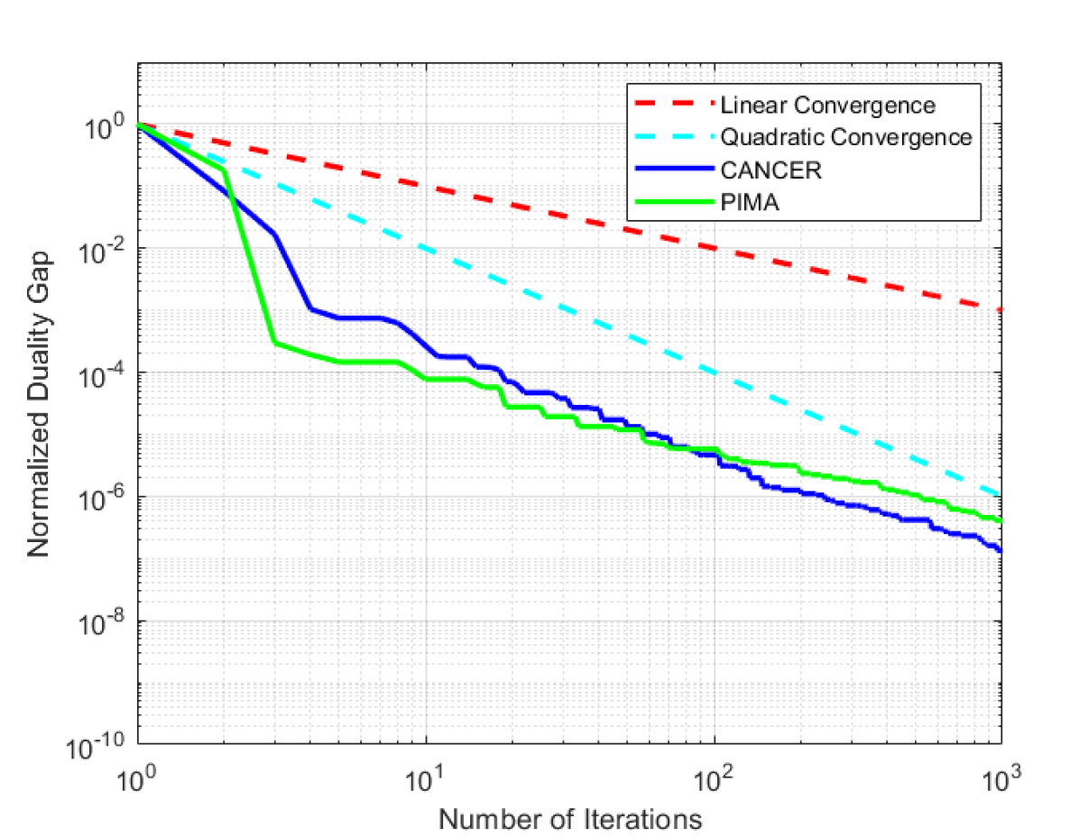
(a) The duality gap for 1000 iterations of FW Algorithm 2, applied to two different classification data sets.

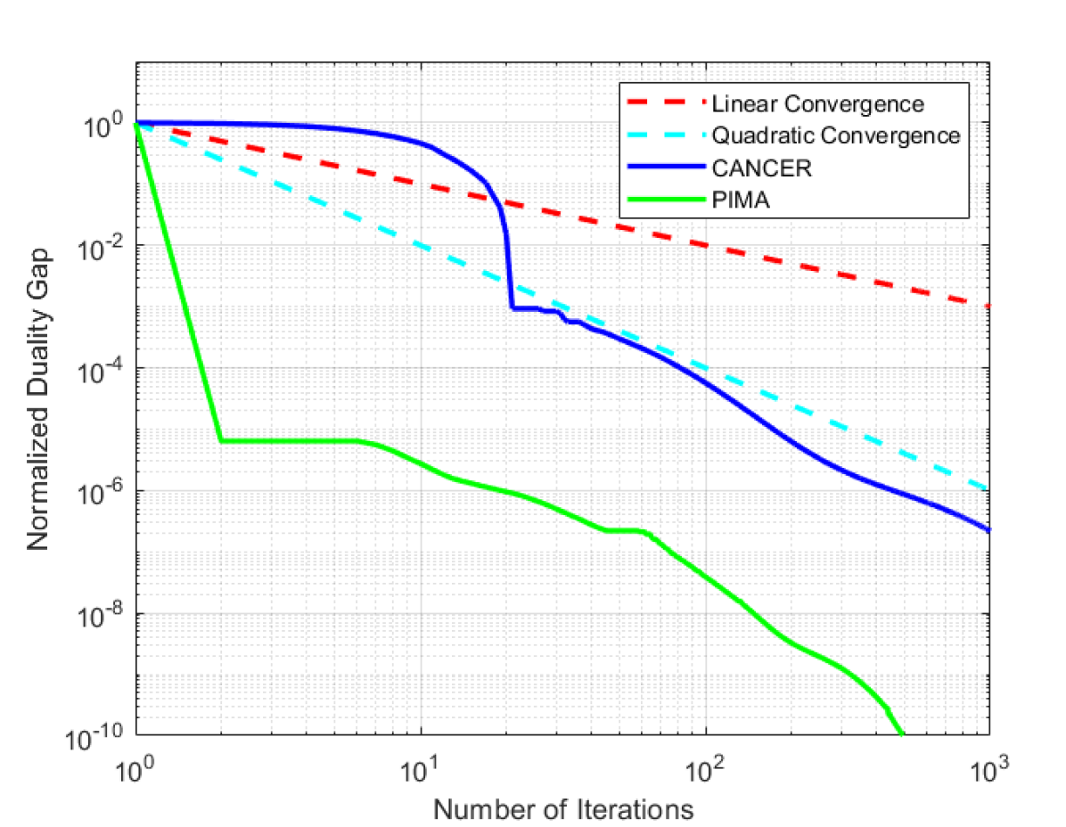
(b) The duality gap for 1000 iterations of APD Algorithm, applied to two different classification data sets.

Figure 1: Convergence rates of the Franke-Wolfe algorithm 1 and the alternative APD algorithm described in Subsection 5.5. In (a) we plot the gap between $OPT\_A(P_{k})$ and $OPT\_P(\alpha_{k})$ of the Franke-Wolfe Algorithm 1 vs. iteration number; in (b) we again plot the gap between $OPT\_A(P_{k})$ and $OPT\_P(\alpha_{k})$ vs. iteration number for the APD Algorithm and in (c) we plot the boosted algorithm. Both demonstrate quadratic convergence, but with enhanced performance for the hybrid algorithm.

7 Numerical Convergence and Scalability

The computational complexity of the algorithms proposed in this paper will depend both on the computational complexity required to perform each iteration as well as the number of iterations required to achieve a desired level of accuracy. In this section, we use numerical tests to determine the observed convergence rate of Algorithm 2 and the observed computational complexity of each iteration when applied to several commonly used machine learning data sets.

7.1 Convergence Properties

In this subsection, we briefly consider the estimated number of iterations of the FW algorithm 1 required to achieve a given level of accuracy as measured by the gap between the primal and dual solutions. Primal-Dual algorithms such as the proposed FW method typically achieve high rates of convergence. While the number of iterations required to achieve a given level of accuracy does not typically change with the size or type of the problem, if the number of iterations required to achieve convergence is excessive, this will have a significant impact on the performance of the algorithm. In Section 5, we established that the proposed algorithm has worst-case linear convergence and proposed an alternative ADP approach with provable quadratic performance. However, provable bounds on convergence rates are often conservative and in this subsection we examine the observed convergence rates as applied to several test cases in both the classification and regression frameworks.

First, to study the convergence properties of the FW Algorithm 2, in Figure 1(a), we plot the gap between $OPT\_A(P_{k})$ and $OPT\_P(\alpha_{k})$ as a function of iteration number for the CANCER and PIMA data sets. The use of the $OPT\_A(P_{k})$-$OPT\_P(\alpha_{k})$ gap for an error metric is a slight improvement over typical implementations of the FW error metric – which uses a predicted bound on the primal-dual gap. However, in practice, we find that the observed convergence rate does not change significantly depending on which metric is used. For reference, Fig. 1 also includes a plot of theoretical worst-case linear and quadratic convergence. As is common in primal-dual algorithms, we observe that the achieved convergence rates significantly exceed the provable linear bound, with this difference being especially noticeable for the first few iterations. These results indicate that for a moderate level of accuracy, the performance of the FW algorithm is adequate – especially combined with the low per-iteration complexity described in the following subsection. However, benefits of the FW algorithm are more limited at high levels of accuracy. Thus, in Fig.  1 (b), we find convergence rates for the suggested APD algorithm mentioned in Subsection 5.5. Unlike the FW algorithm, convergence rates for the first few iterations of APD are not uniformly high. This observation, combined with a slightly higher per-iteration complexity of APD is the reason for our focus on the FW implementation. However, as noted in Appendix B , these algorithms can be combined by switching to the APD algorithm after a fixed number of iterations – an approach which offers superior convergence when desired accuracy is high.

7.2 Computational Complexity

(a) Iteration complexity for the FW algorithm applied to classification

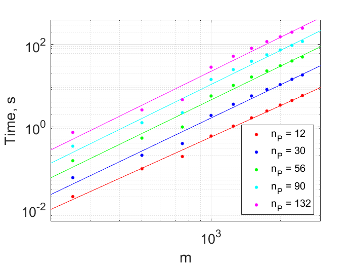
(b) Iteration complexity for the APD algorithm applied to classification

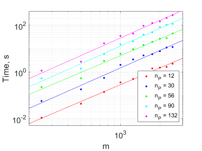
(c) Iteration complexity for the FW algorithm applied to regression

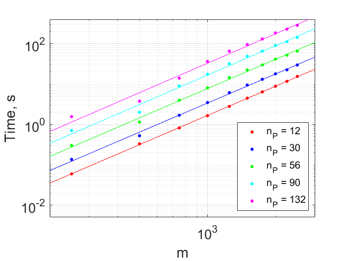
(d) Iteration complexity for the APD algorithm applied to regression

Figure 2: Per-iteration complexity of the proposed FW algorithm 1 and the alternative APD algorithm described in Subsection 5.5. In (a) and (c) we find log-log plots of iteration complexity of the Franke Wolfe (FW) TKL classification and regression algorithms, respectively, ad a function of $m$ for several values of $n_{P}$. Here $m$ is number of samples and $n_{P}^{2}$ is the number of parameters in $\mathcal{K}$, so that $P\in\mathbb{S}^{n_{P}}$. In (b) and (b) we find log-log plots of iteration complexity of the Accelerated Primal Dual (APD) for classification and regression, respectively as a function of $m$ for several values of $n_{P}$. In both cases, best linear fit is included for reference.

Method	Liver	Cancer	Heart	Pima
SDP	95.75 $\pm$ 2.68	636.17 $\pm$ 25.43	221.67 $\pm$ 29.63	1211.66 $\pm$ 27.01
Algorithm 2	0.12 $\pm$ 0.03	0.41 $\pm$ 0.23	4.71 $\pm$ 1.15	0.80 $\pm$ 0.36

Table 1: The mean computation time (in seconds), along with standard deviation, for 30 trials comparing the SDP algorithm in Colbert and Peet (2020a) and Algorithm 2. All tests are run on an Intel i7-5960X CPU at 3.00 GHz with 128 Gb of RAM.

In Figures 2(a-d), we plot the computation time of a single iteration of the FW TKL and APD algorithms for both classification and regression on an Intel i7-5960X CPU with 128 Gb of RAM as a function of $m$ for several values of $n_{P}$, where $m$ is the number of samples used to learn the TK kernel function and the size of $P$ is $n_{P}\times n_{P}$ (so that $n_{P}$ is a function of the number of features and the degree of the monomial basis $Z_{d}$). The data set used for these plots is California Housing (CA) in Pace and Barry (1997b), containing 9 features and $m=20,640$ samples. In the case of classification, labels with value greater than or equal to the median of the output were relabeled as $1$, and those less than the median were relabeled as $-1$. Figures 2(a-d) demonstrate that the complexity of Algorithm 2 (Algorithm 4) scales as approximately $O(m^{2.6}n_{P}^{1.8})$ ($O(m^{2.7}n_{P}^{1.6})$ ) for classification and $O(m^{2.4}n_{P}^{1.9})$ ($O(m^{2.4}n_{P}^{1.2})$) for regression. While this complexity scaling is consistent with theoretical bounds, and while the difference in iteration complexity between the FW and APD algorithms for these data sets is minimal, we find significant differences in scaling between data sets. Furthermore, we find that for similar scaling factors, the FW iteration is approximately 3 times faster than the APD iteration. This multiplicative factor increases to 100 when compared to the SDP algorithm in Colbert and Peet (2020a). This factor is illustrated for classification using four data sets in Table 1

8 Accuracy of the New TK Kernel Learning Algorithm

In this section, we compare the accuracy of the classification and regression solutions obtained from the FW TKL algorithm with $N$ as defined in Eq. (11) to the accuracy of SimpleMKL, Neural Networks, Random Forest, and XGBoost algorithms. In the case of classification we also include three algorithms from the MKLpy python toolbox (AMKL, PWMK, and CKA).

References to the original sources for the data sets used in Section 8 of the paper are included in Table 2. Six classification and six regression data sets were chosen randomly from Dua and Graff (2017) and Chang and Lin (2011) to contain a variety of number of features and number of samples. In both classification and regression, the accuracy metric uses 5 random divisions of the data into test sets ($m_{t}$ samples $\cong 20$% of data) and training sets ($m$ samples $\cong 80$% of data). For regression, the training data is used to learn the kernel and predictor. The predictor is then used to predict the test set outputs.

Name	Type	Source	References
Liver	Classification	UCI	McDermott and Forsyth (2016)
Cancer	Classification	UCI	Wolberg et al. (1990)
Heart	Classification	UCI	No Associated Publication
Pima	Classification	UCI	No Associated Publication
Hill Valley	Classification	UCI	No Associated Publication
Shill Bid	Classification	UCI	Alzahrani and Sadaoui (2018, 2020)
Abalone	Classification	UCI	Waugh (1995)
Transfusion	Classification	UCI	Yeh et al. (2009)
German	Classification	LIBSVM	No Associated Publication
Four Class	Classification	LIBSVM	Ho and Kleinberg (1996)
Gas Turbine	Regression	UCI	Kaya et al. (2019)
Airfoil	Regression	UCI	Brooks et al. (1989)
CCPP	Regression	UCI	Tüfekci (2014); Kaya et al. (2012)
CA	Regression	LIBSVM	Pace and Barry (1997b)
Space	Regression	LIBSVM	Pace and Barry (1997a)
Boston Housing	Regression	LIBSVM	Harrison and Rubinfeld (1978)

Table 2: References for the data sets used in Section 8. All data sets are available on the UCI Machine Learning Repository or from the LIBSVM database.

Regression analysis

Using six different regression data sets, the MSE accuracy of the proposed algorithm (TKL) with $N$ as defined in Eq. (11) was below average on five of the data sets, an improvement over all other algorithms but XGBoost which also scored above average on five of the data sets. To evaluate expected improvement in accuracy, we next compute the average MSE improvement for TKL averaged over all algorithms and data sets to be $23.6\%$ – i.e.

$$\frac{1}{6}\sum_{j=1}^{6}\frac{MSE_{TKL,Dataset(j)}}{\frac{1}{5}\sum_{i=1}^{5}MSE_{Algorithm(i),Dataset(j)}}\cdot 100=100\%-23.6\%$$

This improvement in average performance was better than all other tested algorithms including XGBoost.

Predictably, the computational time of TKL is significantly higher than non-convex non-kernel-based approaches such as RF or XGBoost. However, the computation time of TKL is lower than other kernel-learning methods such as SMKL – note that for large datasets ($m>5000$) TKL is at least 20 times faster than SMKL. Surprisingly, the computation time of TKL is comparable to over-parameterized non-convex stochastic descent methods such as NNet.

Data set	Method	Error	Time (s)	Data set	Method	Error	Time (s)
Gas	TKL	0.23 $\pm$ 0.01	13580 $\pm$ 2060	CCPP	TKL	10.57 $\pm$ 0.82	626.7 $\pm$ 456.0
Turbine	SMKL	N/A	N/A	$n$ = 4	SMKL	13.93 $\pm$ 0.78	13732 $\pm$ 1490
$n$ = 11	NNet	0.27 $\pm$ 0.03	1172 $\pm$ 100	$m$ = 8000	NNet	15.20 $\pm$ 1.00	305.71 $\pm$ 9.25
$m$ = 30000	RF	0.38 $\pm$ 0.02	16.44 $\pm$ 0.57	$m_{t}$ = 1568	RF	10.75 $\pm$ 0.70	1.65 $\pm$ 0.19
$m_{t}$ = 6733	XGBoost	0.33 $\pm$ 0.005	49.46 $\pm$ 1.93		XGBoost	8.98 $\pm$ 0.81	5.47 $\pm$ 2.73
Airfoil	TKL	1.41 $\pm$ 0.44	49.87 $\pm$ 4.29	CA	TKL	.012 $\pm$ .0003	1502 $\pm$ 2154
$n$ = 5	SMKL	4.33 $\pm$ 0.79	617.8 $\pm$ 161.6	$n=8$	SMKL	N/A	N/A
$m$ = 1300	NNet	6.06 $\pm$ 3.84	211.9 $\pm$ 41.0	$m=16500$	NNet	.0113 $\pm$ .0004	914.3 $\pm$ 95.9
$m_{t}$ = 203	RF	2.36 $\pm$ 0.42	0.91 $\pm$ 0.20	$m_{t}=4140$	RF	.0096 $\pm$ .0003	5.28 $\pm$ 3.13
	XGBoost	1.51 $\pm$ 0.40	2.59 $\pm$ 0.06		XGBoost	.0092 $\pm$ .0002	5.28 $\pm$ 3.13
Space	TKL	.013 $\pm$ .001	121.8 $\pm$ 49.2	Boston	TKL	10.36 $\pm$ 5.80	63.05 $\pm$ 2.90
$n$ = 12	SMKL	.019 $\pm$ .005	3384 $\pm$ 589	Housing	SMKL	15.46 $\pm$ 11.49	10.39 $\pm$ 0.89
$m$ = 6550	NNet	.014 $\pm$ .004	209.7 $\pm$ 37.4	$n$ = 13	NNet	50.90 $\pm$ 44.19	79.2 $\pm$ 42.8
$m_{t}$ = 1642	RF	.017 $\pm$ .003	1.06 $\pm$ 0.27	$m$ = 404	RF	10.27 $\pm$ 5.70	0.68 $\pm$ 0.40
	XGBoost	.015 $\pm$ .002	0.32 $\pm$ 0.02	$m_{t}$ = 102	XGBoost	9.40 $\pm$ 4.17	0.14 $\pm$ 0.06

Table 3: Regression performance of Tessellated Kernel learning for 6 regression data sets with comparison of 5 different ML algorithms. Each measurement was repeated 5 times. The resulting test Mean Squared Error (MSE) and training time are included in the table. All tests are run on a desktop with Intel i7-5960X CPU at 3.00 GHz and with 128 Gb of RAM. N/A indicates that the algorithm was stopped after 24 hours without a solution. For each data set. the number of samples, $m$, the size of the test part $m_{t}$ and the number of features, $n$, are presented.

Classification analysis

Using six classification data sets and comparing 7 algorithms, the TSA of the proposed TKL algorithm was above average on all of the data sets, an improvement over all other algorithms. Next, we compute the average improvement in accuracy of TKL over average TSA for all algorithms to be 6.77$\%$ – i.e.

$$\frac{1}{6}\sum_{j=1}^{6}\frac{TSA_{TKL,Dataset(j)}}{\frac{1}{8}\sum_{i=1}^{8}TSA_{Algorithm(i),Dataset(j)}}\cdot 100=100\%+6.77\%$$

This was close to the top score of 6.84$\%$ achieved by the AMKL algorithm (The PWMK algorithm failed to converge on one dataset, and the TSA from this test was not included in the calculation).

Again, the computational time of TKL is significantly higher than RF or XGBoost, but comparable to other kernel learning methods and NNet. Unlike TKL, the computational time of other MKL methods is highly variable and often does not seem to scale predictably with the number of samples and features – e.g. PWMK for FourClass and Shill Bid data sets and AMKL for Transfusion and German, where the computational time is much higher for smaller datasets.

Details of the Implementation of the algorithms used in this study are as follows.

Data set	Method	Accuracy (%)	Time (s)	Data set	Method	Accuracy (%)	Time (s)
Abalone	TKL	84.61 $\pm$ 1.60	17.63 $\pm$ 3.77	Hill Valley	TKL	86.70 $\pm$ 5.49	86.7 $\pm$ 48.2
$n$ = 8	SMKL	83.13 $\pm$ 1.06	350.4 $\pm$ 175.1	$n$ = 100	SMKL	51.23 $\pm$ 3.55	2.81 $\pm$ 2.83
$m$ = 4000	NNet	84.70 $\pm$ 1.82	4.68 $\pm$ 0.64	$m$ = 1000	NNet	70.00 $\pm$ 4.79	3.79 $\pm$ 1.75
$m_{t}$ = 677	RF	84.11 $\pm$ 1.33	0.98 $\pm$ 0.21	$m_{t}$ = 212	RF	56.04 $\pm$ 3.27	0.75 $\pm$ 0.33
	XGBoost	82.69 $\pm$ 1.06	0.20 $\pm$ 0.06		XGBoost	55.66 $\pm$ 2.37	0.58 $\pm$ 0.34
	AMKL	84.64 $\pm$ 1.01	0.95 $\pm$ 0.07		AMKL	94.71 $\pm$ 1.72	5.50 $\pm$ 3.84
	PWMK	84.64 $\pm$ 1.01	3.13 $\pm$ 0.12		PWMK	94.34 $\pm$ 1.69	13.10 $\pm$ 5.19
	CKA	65.05 $\pm$ 0.76	21.43 $\pm$ 0.32		CKA	47.92 $\pm$ 0.57	0.50 $\pm$ 0.08
Transfusion	TKL	77.84 $\pm$ 3.89	0.25 $\pm$ 0.08	Shill Bid	TKL	99.76 $\pm$ 0.08	23.66 $\pm$ 2.63
$n$ = 4	SMKL	76.62 $\pm$ 4.79	2.44 $\pm$ 3.08	$n$ = 9	SMKL	97.71 $\pm$ 0.32	81.0 $\pm$ 13.1
$m$ = 600	NNet	78.78 $\pm$ 3.26	1.01 $\pm$ 0.47	$m$ = 5000	NNet	98.64 $\pm$ 0.86	3.56 $\pm$ .60
$m_{t}$ = 148	RF	75.00 $\pm$ 3.58	0.54 $\pm$ 0.24	$m_{t}$ = 1321	RF	99.35 $\pm$ 0.14	0.78 $\pm$ 0.36
	XGBoost	73.92 $\pm$ 3.95	0.13 $\pm$ 0.11		XGBoost	99.61 $\pm$ 0.06	0.13 $\pm$ 0.04
	AMKL	74.46 $\pm$ 1.50	766.9 $\pm$ 315.4		AMKL	99.72 $\pm$ 0.10	1.24 $\pm$ 0.04
	PWMK	N/A	N/A		PWMK	99.72 $\pm$ 0.10	3.03 $\pm$ 0.04
	CKA	76.35 $\pm$ 4.27	0.18 $\pm$ 0.03		CKA	99.65 $\pm$ 0.21	55.8 $\pm$ 0.9
German	TKL	75.80 $\pm$ 1.89	58.7 $\pm$ 36.1	FourClass	TKL	99.77 $\pm$ 0.32	0.13 $\pm$ 0.01
$n$ = 24	SMKL	74.30 $\pm$ 3.55	17.78 $\pm$ 4.79	$n$ = 2	SMKL	94.53 $\pm$ 12.2	0.85 $\pm$ 0.48
$m$ = 800	NNet	72.70 $\pm$ 3.98	0.61 $\pm$ 0.05	$m$ = 690	NNet	99.99 $\pm$ 0.01	0.53 $\pm$ 0.03
$m_{t}$ = 200	RF	74.90 $\pm$ 1.35	0.64 $\pm$ 0.28	$m_{t}$ = 172	RF	99.30 $\pm$ 0.44	0.68 $\pm$ 0.53
	XGBoost	72.40 $\pm$ 2.89	0.10 $\pm$ 0.03		XGBoost	98.95 $\pm$ 0.44	0.04 $\pm$ 0.00
	AMKL	70.80 $\pm$ 1.47	2.88 $\pm$ 0.38		AMKL	99.99 $\pm$ 0.01	1.39 $\pm$ 0.03
	PWMK	70.70 $\pm$ 1.50	907.0 $\pm$ 77.6		PWMK	99.99 $\pm$ 0.01	990 $\pm$ 60.2
	CKA	68.50 $\pm$ 1.58	0.25 $\pm$ 0.03		CKA	66.16 $\pm$ 3.44	0.16 $\pm$ 0.03

Table 4: Classification performance of Tessellated Kernel learning for 6 different classification data sets with comparison of 7 ML methods. Each measurement was repeated 5 times. The resulting Test Set Accuracy and training time are presented in the table. All tests are run on a desktop with Intel i7-5960X CPU at 3.00 GHz and with 128 Gb of RAM. N/A indicates that the algorithm was stopped after 24 hours without a solution. For each data set. the number of samples, $m$, the size of the test part $m_{t}$ and the number of features, $n$, are presented.

[TKL] Algorithm 2 with $N$ as defined in Eqn. (11), where $Z_{d}$ is a vector of monomials of degree $d=1$ or less. The regression problem is posed using $\epsilon=.1$. The data is scaled so that $x_{i}\in[0,1]^{n}$ and $[a,b]=[0-\delta,1+\delta]^{n}$, where $\delta\geq 0$ and $C$ in the kernel learning problem are chosen by 2-fold cross-validation. Implementation and documentation of this method is described in Appendix C.1 and is publicly available via Github (Colbert et al., 2021);

[SMKL] SimpleMKL proposed in Rakotomamonjy et al. (2008) with a standard selection of Gaussian and polynomial kernels with bandwidths arbitrarily chosen between .5 and 10 and polynomial degrees one through three - yielding approximately $13(n+1)$ kernels. The regression and classification problems are posed using $\epsilon=.1$ and $C$ is chosen by 2-fold cross-validation;

[NNet] A neural network with 3 hidden layers of size 50 using MATLAB’s patternnet for classification and feedforwardnet for regression where learning is halted after the error in a validation set decreased sequentially 50 times;

[RF] The Random Forest algorithm as in Breiman (2004) as implemented on the scikit-learn python toolbox (see Pedregosa et al., 2011)) for classification and regression. Between 50 and 650 trees (in 50 tree intervals) are selected using 2-fold cross-validation;

[XGBoost] The XGBoost algorithm as implemented in Chen and Guestrin (2016) for classification and regresion. Between 50 and 650 trees (in 50 tree intervals) are selected using 2-fold cross-validation;

[AMKL] The AverageMKL implementation from the MKLpy python package proposed in Lauriola and Aiolli (2020) – averages a standard selection of Gaussian and polynomial kernels;

[PWMK] The PWMK implementation from the MKLpy python package proposed in Lauriola and Aiolli (2020), which uses a heuristic based on individual kernel performance as in Tanabe et al. (2008) to learn the weights of a standard selection of Gaussian and polynomial kernels;

[CKA] The CKA implementation from the MKLpy python package (Lauriola and Aiolli, 2020), uses the centered kernel alignment optimization in closed form as in Cortes et al. (2010) to learn the weights of a standard selection of Gaussian and polynomial kernels.

To further illustrate the importance of density property and the TKL framework for practical regression problems, Algorithm 2 with $N=N_{2}^{T}$ was applied to elevation data from Becker et al. (2009) to learn a SVM predictor representing the surface of the Grand Canyon in Arizona. This data set is particularly challenging due to the variety of geographical features. The results can be seen in Figure 3(d) where we see that the regression surface visually resembles a photograph of this terrain, avoiding the artifacts present in the SVM from an optimized Gaussian kernel seen in Figure 3(c).

(a) An image from Google Maps of a section of the Grand Canyon corresponding to (36.04, -112.05) latitude and (36.25, -112.3) longitude.

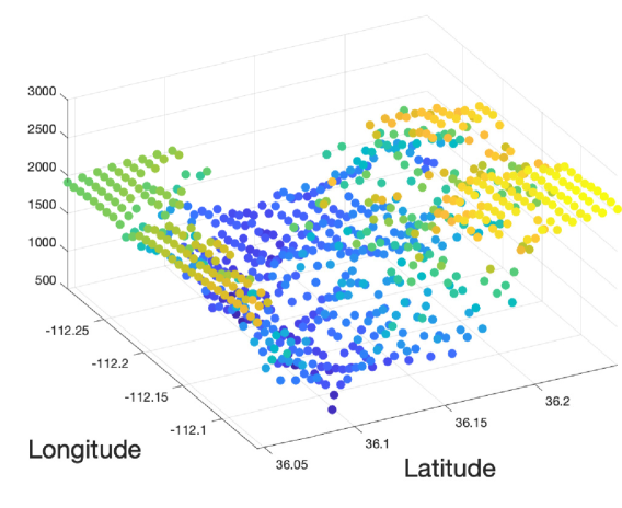
(b) Elevation data ($m=750$) from Becker et al. (2009) for a section of the Grand Canyon between (36.04, -112.05) latitude and (36.25, -112.3) longitude.

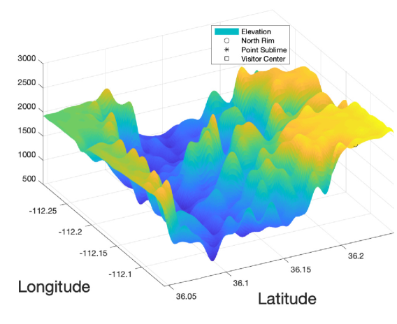
(c) Predictor using a hand-tuned Gaussian kernel trained on the elevation data in (b). The Gaussian predictor poorly represents the sharp edge at the north and south rim.

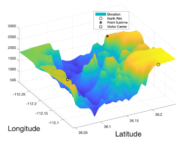
(d) Predictor from Algorithm 2 trained on the elevation data in (b). The TK predictor accurately represents the north and south rims of the canyon.

Figure 3: Subfigure (a) shows an 3D representation of the section of the Grand Canyon to be fitted. In (b) we plot elevation data of this section of the Grand Canyon. In (c) we plot the predictor for a hand-tuned Gaussian kernel. In (d) we plot the predictor from Algorithm 2 for $d=2$.

9 Conclusion

We have proposed a generalized kernel learning framework – using positive matrices to parameterize positive kernels. While such problems can be solved using semidefinite programming, the use of SDP results in large computational overhead. To reduce this computational complexity, we have proposed a saddle-point formulation of the generalized kernel learning problem. This formulation leads to a primal-dual decomposition, which can then be solved efficiently using algorithms of the Frank-Wolfe or accelerated primal dual type – with corresponding theoretical guarantees of convergence. In both cases, we have shown that the primal and dual sub-problems can be solved using a singular value decomposition and quadratic programming, respectively. Numerical experiments confirm that the FW-based algorithm is approximately 100 times faster than the previous SDP algorithm from Colbert and Peet (2020a). Finally, 12 large and randomly selected data sets were used to test accuracy of the proposed algorithms compared to 8 existing state-of-the-art alternatives – yielding uniform increases in accuracy with similar or reduced computational complexity.

Acknowledgments

We would like to acknowledge support for this project from the National Science Foundation (NSF grant NIH DMS/NIGMS-2054354).

A Proof of Universality of Tessellated Kernels

In this appendix, we find a detailed proof of Lemma 14.

Lemma 14

For any $a,b,\delta\in\mathbb{R}^{n}$ with $a<b$ and $\delta>0$, let $Y=[a-\delta,b+\delta]$ and $X=[a,b]$. Then the kernel

$$k(x,y) =\int_{Y}\mathbf{I}(z-x)\mathbf{I}(z-y)dz=\int_{\begin{subarray}{c}x\leq z\\ y\leq z\\ z\leq b+\delta\\ \end{subarray}}1dz=\prod_{i=1}^{n}(b_{i}+\delta_{i}-\max{\{x_{i},y_{i}\}})=\prod_{i=1}^{n}k_{i}(x_{i},y_{i})$$

is universal where $k_{i}(x,y):=b_{i}+\delta_{i}-\max{\{x_{i},y_{i}\}}$.

Proof  As per Micchelli et al. (2006), $k:X\times X\rightarrow\mathbb{R}$ is universal if it is continuous and, if for any $g\in\mathcal{C}(X)$ and any $\epsilon>0$ there exist $f\in\mathcal{H}$ such that $\lVert{f-g}\rVert_{\mathcal{C}}\leq\epsilon$ where

$$\mathcal{H}:=\{f\;:\;f(x)=\sum_{i=1}^{m}\alpha_{i}k(x,y_{i})\;:\;y_{i}\in X,\;\alpha_{i}\in\mathbb{R},\;m\in\mathbb{N}\}.$$

First, we show that each kernel, $k_{i}(x,y)$, with corresponding RKHS $\mathcal{H}_{i}$, is universal for $i=1,\cdots,n$. As shown in Colbert and Peet (2020a), any triangle function, $\Lambda$, of height $1$, of width $2\beta$, and centered at $y_{2}\in[a_{i}+\beta,b_{i}-\beta]$, is in $\mathcal{H}_{i}$, since

$$\Lambda(x)=\sum_{j=1}^{3}\alpha_{j}k_{i}(x,y_{j})=\begin{cases}0,&\text{ if }x<y_{1}\\ \frac{1}{\beta}(x-y_{1}),&\text{ if }y_{1}\leq x<y_{2}\\ 1-\frac{1}{\beta}(x-y_{2}),&\text{ if }y_{2}\leq x<y_{3}\\ 0,&\text{ if }y_{3}\leq x\\ \end{cases}$$

where $y_{1}=y_{2}-\beta$, $y_{3}=y_{2}+\beta$ and $\alpha_{1}=\alpha_{3}=-\frac{1}{\beta}$, $\alpha_{2}=2\frac{1}{\beta}$. Furthermore, using $\alpha_{1}=\frac{1}{\delta}$ and $y_{1}=b_{i}$, we have $\alpha_{1}k_{i}(x,y_{1})=\frac{1}{\delta}k_{i}(x,b_{i})=1$ and so the constant function $\Lambda=1$ is also in $\mathcal{H}_{i}$. Thus we conclude that $\mathcal{H}_{i}$ contains the Schauder basis for $\mathcal{C}([a_{i},b_{i}])$ (See Hunter and Nachtergaele, 2001) and hence the kernel is universal for $n=1$.

Next, since $k=\prod_{i=1}^{n}k_{i}$, we have that

$$\mathcal{H}=\left\{\prod_{i=1}^{n}f_{i}\;:\;f_{i}\in\mathcal{H}_{i}\right\}.$$

Thus, since the $k_{i}$ are universal, for any for any $\gamma\in\mathbb{N}^{n}$ and $x_{i}^{\gamma_{i}}$, there exist $g_{i}\in\mathcal{H}_{i}$ such that $|x_{i}^{\gamma_{i}}-g_{i}(x_{i})|\leq\epsilon$.

Note that $g_{i}(x_{i})$ are bounded, indeed define $C_{i}:=(\max\{|a_{i}|,|b_{i}|\})^{\gamma_{i}}+1$ and $C:=\prod_{i=1}^{n}C_{i}$, then

$$\sup_{x_{i}\in[a_{i},b_{i}]}|g_{i}(x_{i})|\leq\sup_{x_{i}\in[a_{i},b_{i}]}|x_{i}^{\gamma_{i}}|+\epsilon\leq((\max\{|a_{i}|,|b_{i}|\})^{\gamma_{i}}+\epsilon\leq(\max\{|a_{i}|,|b_{i}|\})^{\gamma_{i}}+1=C_{i}.$$

According to Hardy et al. (1952), for all $a_{i},b_{i}\in\mathbb{R}$ such that $|a_{i}|\leq 1$ and $|b_{i}|\leq 1$, we have that $\left|\prod_{i=1}^{n}a_{i}-\prod_{i=1}^{n}b_{i}\right|\leq\sum_{i=1}^{n}|a_{i}-b_{i}|$. Let $g(x)=\prod_{i=1}^{n}g_{i}(x_{i})$. Then, since $\left|\frac{g_{i}(x_{i})}{C_{i}}\right|\leq 1$, $\left|\frac{x_{i}^{\gamma_{i}}}{C_{i}}\right|\leq 1$ and $C_{i}>1$, we have that

$$\sup_{x\in X}\left|x^{\gamma}-g(x)\right| =\sup_{x\in X}\left|\prod_{i=1}^{n}x_{i}^{\gamma_{i}}-\prod_{i=1}^{n}g_{i}(x_{i})\right|$$

$$=C\sup_{x\in X}\left|\prod_{i=1}^{n}\frac{x_{i}^{\gamma_{i}}}{C_{i}}-\prod_{i=1}^{n}\frac{g_{i}(x_{i})}{C_{i}}\right|$$

$$\leq C\sum_{i=1}^{n}\left|\frac{x_{i}^{\gamma_{i}}}{C_{i}}-\frac{g_{i}(x_{i})}{C_{i}}\right|$$

$$\leq nC\max_{i\in\{1,\cdots,n\}}|x_{i}^{\gamma_{i}}-g_{i}(x_{i})|\leq nC\epsilon.$$

We conclude that for any $\gamma\in\mathbb{N}^{n}$, $\lambda_{\gamma}\in\mathbb{R}$ and $\varepsilon>0$, there exists $\{\alpha_{\gamma,j}\}_{j=1}^{m_{\gamma}}$ and $\{y_{\gamma,j}\}_{j=1}^{m_{\gamma}}$ such that

$$\sup_{x\in X}\Biggl{\lVert}{\sum_{j=1}^{m_{\gamma}}\alpha_{\gamma,j}k(x,y_{\gamma,j})-\lambda_{\gamma}x^{\gamma}}\Biggr{\rVert}\leq\varepsilon.$$

Now, the Weierstrass approximation theorem (Willard, 2012) states that polynomials as a linear combination of monomials are dense in $\mathcal{C}(X)$. Thus for any $f\in\mathcal{C}(X)$ and $\varepsilon>0$ there exists a maximal degree $d\in\mathbb{N}$ and a polynomial function $p(x)=\sum_{\|\gamma\|_{1}\leq d}\lambda_{\gamma}x^{\gamma}$ such that

$$\sup_{x\in X}\Bigl{\lVert}{f(x)-p(x)}\Bigr{\rVert}\leq\varepsilon.$$

Let $\{\alpha_{\gamma,j}\}_{j=1}^{m_{\gamma}}$ and $\{y_{\gamma,j}\}_{j=1}^{m_{\gamma}}$ be as defined above. Then, using the triangle inequality, we have

$$\sup_{x\in X}\Biggl{\lVert}{f(x)-\sum_{\|\gamma\|_{1}\leq d}\sum_{j=1}^{m_{\gamma}}\alpha_{\gamma,j}k(x,y_{\gamma,j})}\Biggr{\rVert} =\sup_{x\in X}\Biggl{\lVert}{f(x)-p(x)+p(x)-\sum_{\|\gamma\|_{1}\leq d}\sum_{j=1}^{m_{\gamma}}\alpha_{\gamma,j}k(x,y_{\gamma,j})}\Biggr{\rVert}$$

$$\leq\sup_{x\in X}\Bigl{\lVert}{f(x)-p(x)}\Bigr{\rVert}+\sup_{x\in X}\Biggl{\lVert}{p(x)-\sum_{\|\gamma\|_{1}\leq d}\sum_{j=1}^{m_{\gamma}}\alpha_{\gamma,j}k(x,y_{\gamma,j})}\Biggr{\rVert}$$

$$\leq\sup_{x\in X}\Bigl{\lVert}{f(x)-p(x)}\Bigr{\rVert}+\sum_{\|\gamma\|_{1}\leq d}\sup_{x\in X}\Biggl{\lVert}{\lambda_{\gamma}x^{\gamma}-\sum_{j=1}^{m_{\gamma}}\alpha_{\gamma,j}k(x,y_{\gamma,j})}\Biggr{\rVert}$$

$$\leq\left(\begin{pmatrix}n+d\\ d\end{pmatrix}+1\right)\varepsilon.$$

Thus, since for any $f\in\mathcal{C}(X)$ and any $\epsilon>0$, there exists $g=\sum_{\|\gamma\|_{1}\leq d}\sum_{j=1}^{m_{\gamma}}\alpha_{\gamma,j}k(x,y_{\gamma,j})$ such that $\lVert{f-g}\rVert_{C}\leq\epsilon$. Therefore, since any $k\in\mathcal{K}_{T}$ is continuous (See Colbert and Peet, 2020a), we have that $k$ is universal.  

B An Accelerated Algorithm for Quadratic Convergence

In this appendix, we consider the Accelerated Primary Dual (APD) algorithm discussed in the main text which can be used to achieve quadratic convergence for Generalized Kernel Learning. First, we define the APD algorithm and prove quadratic convergence. Furthermore, we show that the APD algorithm can be decomposed into primal and dual sub-problems which may be solved using QP and the SVD in a manner similar to the FW algorithm. Finally, we note that the APD algorithm underperforms the proposed FW algorithm for the first several iterations and hence we propose a hybrid algorithm which uses FW until an error tolerance is satisfied and then switched to APD for subsequent iterations.

B.1 An Algorithm with Quadratic Convergence

As discussed in Section 3, the Generalized Kernel Learning problem can be represented as a minmax or saddle point optimization problem (2) which is linear in $P$ and strongly convex in $\alpha$

$$\min_{\alpha\in\mathcal{Y}}\max_{P\in\mathcal{X}}f(\alpha)+\Phi(\alpha)-h(P),$$ (14)

where for Generalized Kernel learning we have that $f(\alpha)=\kappa_{\star}(\alpha)$, $\Phi(\alpha)=\lambda(e_{\star}\odot\alpha)$, and $h(P)=0$ as defined in section 5.

Numerically, we observe that for several first iterations, the Frank-Wolfe GKL algorithm achieves super-linear convergence - which is often sufficient to achieve an error tolerance of $10^{-5}$. However, if lower error tolerances are desired, the linear convergence rate of the FW algorithm at higher iterations can be accelerated by a algorithm with quadratic convergence.

Fortunately, Hamedani and Aybat (2021) has shown that provable quadratic convergence can be achieved using a variation of an algorithm originally proposed in Chambolle and Pock (2016). This algorithm, the accelerated primal-dual (APD) algorithm, requires computation of the same sub-problems, $OPT\_A$ and $OPT\_P$, but it achieves the worst case quadratic convergence.

Specifically, this algorithm can be used to solve problems of the form

$$\min_{\alpha\in\mathcal{Y}_{\star}}\max_{P\in\mathcal{X}}-\kappa_{\star}(\alpha)-O(\alpha\odot e_{\star},P)=f(\alpha)+\Phi(P,\alpha)-h(P),$$ (15)

where $f(\alpha)+\Phi(\alpha)$ is strongly convex and $h(P)$ is concave. Since the Generalized Kernel Learning Problem (GKL (7)) has the same form as problem (15), application of this approach is relatively straightforward. Specifically, consider Algorithm 3 from Hamedani and Aybat (2021) which requires the following definition.

Definition 15 (Bregman distance (Hamedani and Aybat, 2021))

Given $f$ and $h$, let $\phi_{Y}:\mathcal{Y}\rightarrow\mathbb{R}$ and $\phi_{X}:\mathcal{X}\rightarrow\mathbb{R}$ be differentiable functions on open sets $\mathcal{Y}\subset\textbf{dom}\,f$ and $\mathcal{X}\subset\textbf{dom}\,h$. Suppose $\phi_{X}$ and $\phi_{Y}$ have closed domains and are 1-strongly convex with respect to $\|\cdot\|_{\mathcal{X}}$ and $\|\cdot\|_{\mathcal{Y}}$, respectively. We define the Bregman distances $D_{\mathcal{X}}:\mathcal{X}\times\mathcal{X}\rightarrow\mathbb{R}$ and $D_{\mathcal{Y}}:\mathcal{Y}\times\mathcal{Y}\rightarrow\mathbb{R}$ corresponding to $\phi_{X}$ and $\phi_{Y}$, respectively, as $D_{\mathcal{X}}(x,\hat{x})=\phi_{\mathcal{X}}(x)-\phi_{\mathcal{X}}(\hat{x})-\left<\nabla\phi_{\mathcal{X}}(\hat{x}),x-\hat{x}\right>$ and $D_{\mathcal{Y}}(y,\hat{y})=\phi_{\mathcal{Y}}(y)-\phi_{\mathcal{Y}}(\hat{y})-\left<\nabla\phi_{\mathcal{Y}}(\hat{y}),y-\hat{y}\right>$.

  Initialize $\mu,\tau_{0},\sigma_{0}$, $k_{\text{max}}$ and $\alpha_{0},P_{0}\in\mathcal{Y}\times\mathcal{X}$

$k=0$, $(\tau_{-1},\sigma_{-1})=(\tau_{0},\sigma_{0})$, $(P_{-1},\alpha_{-1})=(P_{0},\alpha_{0})$ and $\gamma_{0}=\frac{\sigma_{0}}{\tau_{0}}$;

  while $k<k_{\text{max}}$ do

     1: $\displaystyle\sigma_{k}=\gamma_{k}\tau_{k},\quad\theta_{k}=\sigma_{k-1}/\sigma_{k}$

     2: $x_{k}=\nabla_{P}\Phi(\alpha_{k},P_{k})$

     3: $S=(1+\theta_{k})x_{k}-\theta_{k}x_{k-1}$

     4: $\displaystyle P_{k+1}=\arg\min_{P\in\mathcal{X}}\frac{1}{\sigma_{k}}D_{X}(P,P_{k})-\left<S,P\right>$

     5: $\displaystyle\alpha_{k+1}=\arg\min_{\alpha\in\mathcal{Y}}f(\alpha)+\Phi(P_{k+1},\alpha)+\frac{D_{Y}(\alpha,\alpha_{k})}{\tau_{k}}$

     6: $\gamma_{k+1}=\gamma_{k}(1+\mu\tau_{k})$, $\tau_{k+1}=\tau_{k}\sqrt{\frac{\gamma_{k}}{\gamma_{k+1}}}$, $k=k+1$

  end while

Algorithm 3 APD algorithm

Theorem 16 proves quadratic convergence of Algorithm 3 when $f(\alpha)+\Phi(P,\alpha)$ is strongly convex in $\alpha$ and $h(P)$ is concave.

Theorem 16 (Hamedani and Aybat (2021))

Let $D_{\mathcal{X}}$ and $D_{\mathcal{Y}}$ be Bregman distance functions. Suppose that for and $P\in\mathcal{X}$, $f(\alpha)$ and $\Phi(P,\alpha)$ are convex in $\alpha$ and for any $\alpha\in\mathcal{Y}$, $\Phi(P,\alpha)$ and $-h(P)$ are concave in $P$. In addition, suppose $f$ is strongly convex with modulus $\mu>0$. Furthermore, suppose that $L_{\alpha\alpha},L_{P\alpha}$ satisfy

$$\|\nabla_{P}\Phi(P,\alpha)-\nabla_{P}\Phi(\hat{P},\hat{\alpha})\|_{\mathcal{X^{*}}} \leq L_{P\alpha}\|\alpha-\hat{\alpha}\|_{\mathcal{Y}}$$

$$\|\nabla_{\alpha}\Phi(P,\alpha)-\nabla_{\alpha}\Phi(P,\hat{\alpha})\|_{\mathcal{Y^{*}}} \leq L_{\alpha\alpha}\|\alpha-\hat{\alpha}\|_{\mathcal{Y}}$$

for all $\alpha,\hat{\alpha},P,\hat{P}$ and that the starting parameters $\tau_{0}$ and $\sigma_{0}$ satisfy:

$$\left(\frac{1-\delta}{\tau_{0}}-L_{\alpha\alpha}\right)\frac{1}{\sigma_{0}} \geq\frac{L_{P\alpha}^{2}}{c_{a}}$$

for some $\delta,c_{a}\in\mathbb{R}_{+}$, such that $c_{a}+\delta\leq 1$. If

$$\{\alpha^{*},P^{*}\}=\arg\min_{\alpha\in\mathcal{Y}_{\star}}\max_{P\in\mathcal{X}}f(\alpha)+\Phi(P,\alpha)-h(P),$$

exists, then for any sequence produced by Algorithm 3, $\{\alpha_{k},P_{k}\}$, we have that
1. $\lim_{k\rightarrow\infty}\{P_{k},\alpha_{k}\}\rightarrow\{P^{*},\alpha^{*}\}$
2. if $\delta>0$, and we define $L(\alpha,P):=f(\alpha)+\Phi(P,\alpha)-h(P)$ then

$$0\leq L(P^{*},\alpha_{k})-L(P_{k},\alpha^{*})\leq O\left(\frac{1}{k^{2}}\right).$$

Proof  See Hamedani and Aybat (2021)  
Remark: As stated in Hamedani and Aybat (2021), the conditions of Theorem 16 are satisfied using $\tau_{0}=\frac{1}{3L_{\alpha\alpha}}$ and $\sigma_{0}=\frac{L_{\alpha\alpha}}{2L_{P\alpha}^{2}}$.

B.2 Proposed Booster Algorithm

In this subsection, we propose the following algorithm applicable to our optimization problem. This algorithm is a specification of APD for the Generalized Kernel learning.

  Initialize $(\alpha_{0},P_{0})\in\mathcal{Y}_{\star}\times\mathcal{X}$, $\mu$

$\sigma_{-1}=\sigma_{0}=\frac{L_{\alpha\alpha}}{2L_{\alpha P}^{2}}$, $\tau_{-1}=\tau_{0}=\frac{1}{3L_{\alpha\alpha}}$

$k=0$, $(P_{-1},\alpha_{-1})=(P_{0},\alpha_{0})$ and $\gamma_{0}=\frac{\sigma_{0}}{\tau_{0}}$;

  while $L(P_{k+1},\alpha_{k})-L(P_{k},\alpha_{k+1})>\epsilon$ do

     1: $\displaystyle\sigma_{k}=\gamma_{k}\tau_{k},\quad\theta_{k}=\sigma_{k-1}/\sigma_{k}$

     2: $x_{k}=\frac{1}{2}D(e_{\star}\odot\alpha_{k})$

     3: $S=(1+\theta_{k})x_{k}-\theta_{k}x_{k-1}$

     4: $\displaystyle P_{k+1}=\arg APD\_P(P_{k},S,\sigma_{k})$

     5: $\displaystyle\alpha_{k+1}=\arg APD\_A(\alpha_{k},P_{k+1},\tau_{k})$

     6: $\gamma_{k+1}=\gamma_{k}(1+\mu\tau_{k})$, $\tau_{k+1}=\tau_{k}\sqrt{\frac{\gamma_{k}}{\gamma_{k+1}}}$, $k=k+1$

  end while

Algorithm 4 APD algorithm

where $L(P,\alpha):=-\lambda(e_{\star}\odot\alpha,P)-\kappa_{\star}(\alpha)$ and

$$D_{i,j}(\alpha):=\sum_{k,l=1}^{m}\alpha_{k}e_{*k}G_{i,j}(x_{k},x_{l})\alpha_{l}e_{*l}$$

is defined in Eqn. (12) and the two subroutines $APD\_P$ and $APD\_A$ are defined as

$$APD\_A(P,\alpha_{k},\tau) :=\max_{\alpha\in\mathcal{Y}_{\star}}\lambda(e_{\star}\odot\alpha,P)+\kappa_{\star}(\alpha)-\frac{1}{\tau}D_{\mathcal{Y}}(\alpha,\alpha_{k}),$$

$$APD\_P(P_{k},S,\sigma) :=\min_{P\in\mathcal{X}}\frac{1}{\sigma}D_{\mathcal{X}}(P,P_{k})-\left<S,P\right>$$

where $D_{\mathcal{Y}_{\star}}:=\frac{1}{2}\|\cdot\|_{2}^{2}$, and $D_{\mathcal{X}}:=\frac{1}{2}\|\cdot\|_{F}^{2}$.

Furthermore,

$$\tau_{0}=\frac{1}{3L_{\alpha\alpha}},\;\;\text{and}\;\;\sigma_{0}=\frac{L_{\alpha\alpha}}{2L_{\alpha P}^{2}}$$ (16)

where

$$L_{\alpha\alpha}:=\frac{n_{P}}{2}\sum_{ij}|D_{ij}(e_{\star})|^{2},~{}~{}L_{\alpha P}:=\frac{C}{n_{P}}L_{\alpha\alpha}$$ (17)

where recall that $n_{P}$ is determined by the size of $P$ ($P\in\mathbb{S}^{n_{P}}$) and $C>0$ can be chosen arbitrarily. Finally, we choose $\mu>0$ sufficiently small such that $-\lambda(\alpha\odot e_{\star},P)-\mu\alpha^{T}\alpha$ is convex for all $P\in\mathcal{X}$.

B.3 Quadratic Convergence Proof for Algorithm 4

Formally, we state the theorem.

Theorem 17

Algorithm 4 returns iterates $P_{k}$ and $\alpha_{k}$ such that, $L(\alpha_{k},P_{k+1})-L(\alpha_{k+1},P_{k})<O(\frac{1}{k^{2}})$.

Proof  In this proof, we first show that Algorithm 4 returns iterates $P_{k}$ and $\alpha_{k}$ which satisfy Algorithm 3. Next, we show that if $\tau_{0},\sigma_{0}$ are chosen as per Eqn. (16), then the conditions of Theorem 16 are satisfied. First, let us define

$$f(\alpha) :=-\kappa_{\star}(\alpha)+\mu\alpha^{T}\alpha$$

$$\Phi(P,\alpha) :=-\lambda(\alpha\odot e_{\star},P)-\mu\alpha^{T}\alpha$$ (18)

$$h(P) :=0$$

for some sufficiently small $\mu>0$. Now, suppose that $\{P_{k},\alpha_{k},\gamma_{k},S_{k},x_{k},\sigma_{k},\tau_{k}\}$ satisfy Algorithm 4. Clearly, these iterations also satisfy Steps 1, 3 and 6 of Algorithm 3. Furthermore, these iterations satisfy the equation defined in Step 2 since

$$\nabla_{P} \Phi(\alpha,P)_{ij}=\frac{\partial}{\partial P_{ij}}\left[-\lambda(\alpha\odot e_{\star},P)-\mu\alpha^{T}\alpha\right]$$

$$=\frac{\partial}{\partial P_{ij}}\left[\frac{1}{2}\sum_{i,j=1}^{n_{P}}P_{ij}\sum_{k,l=1}^{m}(\alpha_{k}e_{*k})G_{i,j}(x_{k},x_{l})(\alpha_{l}e_{*l})\right]$$

$$=\frac{1}{2}\sum_{k,l=1}^{m}(\alpha_{k}e_{*k})G_{i,j}(x_{k},x_{l})(\alpha_{l}e_{*l})=\frac{1}{2}D_{ij}(e_{\star}\odot\alpha_{k}).$$

Next, the proposed iterations satisfy the equation defined in Step 4 of Algorithm 3 since by the definition of $APD\_P$

$$P_{k+1} =\arg APD\_P(P_{k},S,\sigma_{k})=\arg\min_{P\in\mathcal{X}}\frac{1}{\sigma_{k}}D_{\mathcal{X}}(P,P_{k})-\left<S,P\right>.$$

Finally the equality in Step 5 of Algorithm 3 is satisfied since

$$\alpha_{k+1}=\arg APD\_A(P_{k+1},\alpha_{k},\tau_{k})$$

$$~{}~{}=\arg\max_{\alpha\in\mathcal{Y}_{\star}}\lambda(e_{\star}\odot\alpha,P_{k+1})+\kappa_{\star}(\alpha)-\frac{1}{\tau_{k}}D_{\mathcal{Y}}(\alpha,\alpha_{k})$$

$$~{}~{}=\arg\min_{\alpha\in\mathcal{Y}_{\star}}-\lambda(e_{\star}\odot\alpha,P_{k+1})-\kappa_{\star}(\alpha)+\frac{1}{\tau_{k}}D_{\mathcal{Y}}(\alpha,\alpha_{k})$$

$$~{}~{}=\arg\min_{\alpha\in\mathcal{Y_{\star}}}f(\alpha)+\Phi(P_{k+1},\alpha)+\frac{1}{\tau_{k}}D_{Y}(\alpha,\alpha_{k}).$$

Therefore we have that $\{P_{k},\alpha_{k},\gamma_{k},S_{k},x_{k},\sigma_{k},\tau_{k}\}$ satisfy Algorithm 3.

We next must show that $\Phi$ is concave in $P$, convex in $\alpha$ and $f$ is strongly convex. $P$ is linear in $\Phi$ and thus concave in $P$. As defined, $\Phi$ is convex in $\alpha$ and clearly, $f$ is strongly convex for any $\mu>0$. Since $L_{\alpha\alpha},L_{\alpha P}$ are as defined in Equation (17), then

$$\|\nabla_{P}\Phi(P,\alpha)-\nabla_{P}\Phi(\hat{P},\hat{\alpha})\|_{\mathcal{X^{*}}} \leq L_{P\alpha}\|\alpha-\hat{\alpha}\|_{\mathcal{Y}}$$

$$\|\nabla_{\alpha}\Phi(P,\alpha)-\nabla_{\alpha}\Phi(P,\hat{\alpha})\|_{\mathcal{Y^{*}}} \leq L_{\alpha\alpha}\|\alpha-\hat{\alpha}\|_{\mathcal{Y}}$$

as desired. Finally, we have that if $\tau_{0}$ and $\sigma_{0}$ are as defined in Equation (16), $\delta=\frac{1}{4}$, and $c_{a}=\frac{1}{2}$ , then $c_{a}+\delta\leq 1$ and

$$\left(\frac{1-\delta}{\tau_{0}}-L_{\alpha\alpha}\right)\frac{1}{\sigma_{0}} \geq\frac{L_{P\alpha}^{2}}{c_{a}}$$

as desired.

Therefore, we have by Theorem 16 that

$$0\leq L(P^{*},\alpha_{k})-L(P_{k},\alpha^{*})\leq O\left(\frac{1}{k^{2}}\right),$$

and hence

$$L(\alpha_{k},P_{k+1})-L(\alpha_{k+1},P_{k}) <L(P^{*},\alpha_{k})-L(P_{k},\alpha^{*})\leq O\left(\frac{1}{k^{2}}\right).$$

 
We next define efficient algorithms to solve the subroutines $APD\_P$ and $APD\_D$.

B.4 Solving APD_P

The fourth step of the APD algorithm requires solving $APD\_P$. For arbitrary matrix $S\in\mathbb{S}^{n_{P}}$ this optimization problem is formulated as follows.

$$P_{k+1}=\arg\min_{P\in\mathcal{Y}}\;\;\frac{1}{\sigma_{k}}D_{X}(P,P_{k})-\left<S,P\right>$$ (19)

The following algorithm solves the optimization task 19

  Input $P_{k},S\in\mathbb{S}^{n_{P}}$, $\sigma_{k},\varepsilon>0$ ;

  Set $r=+\infty$ and $A=P_{k}+\sigma_{k}S$,

  Singular Value Decomposition: $A=\sum_{i}\lambda_{i}p_{i}p_{i}^{T}$

  Initialize $y_{l}=\min_{i}\lambda_{i}$ and $y_{u}=\max_{i}\lambda_{i}$;

  while $r>\varepsilon$ do

     1:   $y=\frac{1}{2}(y_{l}+y_{u})$

     2:   $r=\sum_{i}|\lambda_{i}-y|_{+}-n_{P}$

     3:   update $y_{u}=y$ if $r\geq 0$, or $y_{l}=y$ otherwise

  end while

  Return $P=\sum_{i}|\lambda_{i}-y|_{+}p_{i}p_{i}^{T}=\arg APD\_P(P_{k},S,\sigma).$

Algorithm 5 $APD\_P$ Subroutine

Lemma 18

Let the optimization problem be as defined in (19), then the algorithm 5 returns the solution.

Proof  Firstly, we should reformulate Optimization Problem (19) as,

$$\arg\min_{\begin{subarray}{c}P\in\mathbb{S}^{n_{P}}\\ \text{trace}(P)=n_{P}\\ P>0\end{subarray}}\frac{1}{\sigma}D_{X}(P,P_{k})-\left<S,P\right>=\arg\min_{\begin{subarray}{c}P\in\mathbb{S}^{n_{P}}\\ \text{trace}(P)=n_{P}\\ P>0\end{subarray}}\frac{1}{2\sigma}\|P-P_{k}\|_{F}^{2}-\langle S,P\rangle$$

$$=\arg\min_{\begin{subarray}{c}P\in\mathbb{S}^{n_{P}}\\ \text{trace}(P)=n_{P}\\ P>0\end{subarray}}\frac{1}{2\sigma}\langle P-P_{k},P-P_{k}\rangle-2\sigma\langle S,P\rangle=\arg\min_{\begin{subarray}{c}P\in\mathbb{S}^{n_{P}}\\ \text{trace}(P)=n_{P}\\ P>0\end{subarray}}\frac{1}{2\sigma}\|P-(P_{k}+\sigma S)\|_{F}^{2},$$

$$\qquad=\arg\min_{\begin{subarray}{c}P\in\mathbb{S}^{n_{P}}\\ \text{trace}(P)=n_{P}\\ P>0\end{subarray}}\|P-A\|_{F}^{2},$$ (20)

where $A=P_{k}+\sigma S$.

Having reduced $APD\_P$ to a convex distance minimization problems of the form of Eqn. (20). According to  Harada (2018), we use a subroutine defined by Algorithm 5 to solve problem (20) and therefore to find $P_{k+1}$ in Step 4 of Algorithm 4.  

B.5 Solving APD_A

$APD\_A$ is a QP of the form

$$\min_{\begin{subarray}{c}\alpha\in\mathcal{Y}_{\star}\end{subarray}}\;\;\frac{1}{2}\alpha^{T}Q_{*}\alpha+c_{*}^{T}\alpha,$$

where, $c_{*}^{T}\alpha=-\tau\kappa_{\star}(\alpha)-\alpha_{p}^{T}\alpha,$ and $\alpha^{T}Q_{*}\alpha=-\tau\lambda(e_{\star}\odot\alpha,P)+\alpha^{T}\alpha$.

QP’s of this form can be solved using a slight variation of the algorithm proposed in Subsection 5.3.

B.6 The combined solution

We can see that the Frank-Wolfe GKL Algorithm converges quite quickly up to a certain value, but after that the convergence slows down and becomes linear. Moreover, APD algorithm return a smaller objective function after 3000-4000 iterations. But, the pure APD has non-monotonic convergence at the early stage. All this together prompted us to create a combined Frank-Wolfe GKL and APD algorithm. The tolerance for the Frank-Wolfe GKL was chosen according to the numerical results.

  INPUT $\epsilon$ - tolerance;

  1: $(\alpha_{1},P_{1})=\text{Frank Wolfe GKL with tolerance }\epsilon$

  2: $(\alpha_{2},P_{2})=\text{APD with initial guess }\alpha_{1},P_{1}\text{ and desired tolerance}$

  3:   $\alpha=OPT\_A(P_{2})$, $P=P_{2}$

  OUTPUT:  $\alpha$, $P$

Algorithm 6 Final version of GKL

We assume, that the proposed algorithm 6 will show both fast initial convergence and quadratic convergence in the worst case, which is necessary for application to arbitrary data sets.

C Implementation and Documentation of Algorithms

In this appendix material, we have provided a MATLAB implementation of the proposed algorithms which can be used to reproduce the numerical results given in Section 7. The primary executable is PMKL.m. The demo files exampleClassification.m and exampleRegression.m illustrate typical usage of this executable for classification and regression problems respectively. This software is available from Github (Colbert et al., 2021).

C.1 Documentation for Included Software

Also included in the main material are the 5 train and test partitions used for each of the 12 data sets used in the numerical results section of the paper. The code numericalTest.m allows the user to select the data set and run the FW PMKL algorithm on the five partitions to calculate the average and standard deviation of the MSE (for regression) or TSA (for classification).

The PMKL subroutine
PMKL - Positive Matrix Kernel Learning,

>> f = PMKL(x,y,Type,C,params);

yields an optimal solution to the minimax program

$$\min_{P\in\mathcal{X}}\max_{\alpha\in\mathcal{Y}_{\star}}\lambda(e_{\star}\odot\alpha,P)+\kappa_{\star}(\alpha),$$

where $\mathcal{X}:=\{P\in\mathbb{S}^{n_{P}}\;:\;\text{trace}(P)=n_{P},\;P>0\}$,

$$\mathcal{Y}_{c}:=\{\alpha\in\mathbb{R}^{m}\;:\;\alpha^{T}y=0,\;\alpha_{i}\in[0,C]\},\quad\mathcal{Y}_{r}:=\{\alpha\in\mathbb{R}^{m}\;:\;\alpha^{T}e=0,\;\alpha_{i}\in[-C,C]\},$$

and where,

• $\texttt{x}\in\mathbb{R}^{n\times m}$ is a matrix of $n$ rows corresponding to the number of features and $m$ columns corresponding to the number of samples where $x(:,i)$ is the i’th sample,

• $\texttt{y}\in\mathbb{R}^{m}$ ($\texttt{y}\in[-1,1]^{m}$) is a row of outputs (labels) for each of the samples in x where y(:,i) is the i’th output corresponding to the i’th sample x(:,i),

• Type is the string ’Classification’ for classification or ’Regression’ for regression,

• C is the penalty for miss-classifying a point for classification, or for predicting an output with less than $\epsilon$ accuracy for regression,

• params is a structure containing additional optional parameters such as the kernel function (default is the TK function), kernel parameters (degree of monomial basis for TK or GPK kernels), the domain of integration, the $\epsilon$-loss term for regression, the maximum number of iterations and the tolerance,

• The output f is an internal data structure containing the solutions $P^{*}$ and $\alpha^{*}$, as well as the other user selected parameters. This data structure defines the resulting regressor/classifier. This regressor/classifier can be evaluated using the EvaluatePMKL command as described below.

Default parameters of the params structure are

>> params.kernel  = ’TK’
>> params.delta  = .5
>> params.epsilon = .1
>> params.maxit = 100
>> params.tol = .01

where kernel specifies the kernel function to use, delta determines the bounds of integration $[a,b]=[0-\delta,1+\delta]^{n}$, epsilon is the epsilon-loss of the support vector regression problem, maxit is the maximum number of iterations, and tol is the stopping tolerance. The PMKL.m function can be run with only some of the inputs manually specified, as discussed next.

Default Implementation
To run the PMKL algorithm with all default values for the samples x and outputs y and to automatically select the type of problem (classification or regression) the MATLAB command is,

>> f = PMKL(x,y)

where if y only contains two unique values, the algorithm defaults to classification. Otherwise, the algorithm defaults to regression.

Manual Selection of Classification or Regression
To run the PMKL algorithm with all default values, for the samples x and outputs y but manually select the type of problem, the MATLAB command is,

>> f = PMKL(x,y,Type)

where Type = ’Classification’ for classification or ’Regression’ for regression.

Manually Specifying the Penalty C
To run the PMKL algorithm with all default values except for Type and the penalty term C, for the samples x and outputs y the MATLAB command is,

>> f = PMKL(x,y,Type,C)

where the user must select a $\texttt{C}>0$. It is recommended that the value of C be selected via k-fold cross-validation with data split into training and validation sets.

Manually Specifying Additional Parameters
For help generating the params structure we have included the paramsTK.m function which allows the user to generate a params structure for TK kernels as follows.

>> params = paramsTK(degree,delta,epsilon,maxit,tol)

An empty matrix can be used for any input where the default value is desired, and using the paramsTK framework is recommended when modifying the default values.

The Evaluate Subroutine Once the optimal kernel function has been learned, you can evaluate the predicted output of a set of samples using the following function.

>> yPred = evaluatePMKL(f,xTest)

The output of evaluatePMKL are the predicted outputs of the optimal support vector machine, trained on the data $x$ and $y$ with the designated kernel function optimized by the PMKL subroutine.

• The input f is an internal data structure output from the PMKL function.

• $\texttt{xTest}\in\mathbb{R}^{n\times m}$ is a matrix of $n$ rows corresponding to the number of features and $m$ columns corresponding to the number of samples where xTest(:,i) is the i’th sample,

• The output $\texttt{yPred}\in\mathbb{R}^{1\times m}$ is a vector with $m$ columns corresponding to the number of samples in xTest.

References

• Alzahrani and Sadaoui (2018) A Alzahrani and S Sadaoui. Scraping and Preprocessing Commercial Auction Data for Fraud Classification. arXiv preprint arXiv:1806.00656, 2018.
• Alzahrani and Sadaoui (2020) A. Alzahrani and S. Sadaoui. Clustering and Labeling Auction Fraud Data. In Data Management, Analytics and Innovation, pages 269–283. Springer, 2020.
• Becker et al. (2009) J. J. Becker, D. T. Sandwell, W. H. F. Smith, J. Braud, B. Binder, J. L. Depner, D. Fabre, J. Factor, S. Ingalls, S. H. Kim, et al. Global Bathymetry and Elevation Data at 30 arc Seconds Resolution: SRTM30_PLUS. Marine Geodesy, 32(4):355–371, 2009.
• Bertsekas (2016) D. Bertsekas. Nonlinear Programming. Athena Scientific Optimization and Computation Series. Athena Scientific, 2016. ISBN 9781886529052.
• Boehmke and Greenwell (2019) B. Boehmke and B.M. Greenwell. Hands-On Machine Learning with R. Chapman & Hall/CRC The R Series. CRC Press, 2019. ISBN 9781000730432.
• Borgwardt et al. (2006) K. M. Borgwardt, A. Gretton, M. J. Rasch, H. Kriegel, B. Schölkopf, and A. J. Smola. Integrating structured biological data by Kernel Maximum Mean Discrepancy. Bioinformatics, 2006.
• Breiman (2004) L. Breiman. Random Forests. Machine Learning, 45:5–32, 2004.
• Brian and Young (2007) B. Brian and J. G. Young. Implementation of a primal–dual method for SDP on a shared memory parallel architecture. Computational Optimization and Applications, 37(3):355–369, 2007.
• Brooks et al. (1989) T. F. Brooks, D. S. Pope, and M. A. Marcolini. Airfoil Self-noise and Prediction. NASA reference publication. National Aeronautics and Space Administration, Office of Management, Scientific and Technical Information Division, 1989.
• Chambolle and Pock (2016) A. Chambolle and T. Pock. On the ergodic convergence rates of a first-order primal–dual algorithm. Mathematical Programming, 159(1):253–287, 2016.
• Chang and Lin (2011) C-C. Chang and C-J. Lin. LIBSVM: A Library for Support Vector Machines. ACM Transactions on Intelligent Systems and Technology, 2:27:1–27:27, 2011.
• Chen and Guestrin (2016) T. Chen and C. Guestrin. XGBoost: A Scalable Tree Boosting System. In Proceedings of the 22nd ACM SIGKDD International Conference on Knowledge Discovery and Data Mining, 2016.
• Colbert and Peet (2020a) B.K. Colbert and M.M. Peet. A Convex Parametrization of a New Class of Universal Kernel Functions. Journal of Machine Learning Research, 21(45):1–29, 2020a.
• Colbert and Peet (2020b) B.K. Colbert and M.M. Peet. A New Algorithm for Tessellated Kernel Learning. arXiv preprint arXiv:2006.07693, 2020b.
• Colbert et al. (2021) B.K. Colbert, A. Talitckii, and M.M. Peet. Tessellated Kernel Learning. https://github.com/CyberneticSCL/TKL-version-0.9, 2021.
• Cortes et al. (2010) C. Cortes, M. Mohri, and A. Rostamizadeh. Two-Stage Learning Kernel Algorithms. 2010.
• Dua and Graff (2017) D. Dua and C. Graff. UCI machine learning repository, 2017. URL http://archive.ics.uci.edu/ml.
• Fan (1953) K. Fan. Minimax Theorems. Proceedings of the National Academy of Sciences of the United States of America, 39(1):42, 1953.
• Fang et al. (1994) Y. Fang, K.A. Loparo, and X. Feng. Inequalities for the Trace of Matrix Product. IEEE Transactions on Automatic Control, 39(12):2489–2490, 1994.
• Frank and Wolfe (1956) M. Frank and P. Wolfe. An Algorithm for Quadratic Programming. Naval Research Logistics Quarterly, 3(1-2):95–110, 1956.
• Fukumizu et al. (2007) K. Fukumizu, A. Gretton, X. Sun, and B. Schölkopf. Kernel Measures of Conditional Dependence. Advances in Neural Information Processing Systems, 20, 2007.
• Gohberg et al. (2012) I. Gohberg, S. Goldberg, and M. Kaashoek. Basic Classes of Linear Operators. Birkhäuser Basel, 2012. ISBN 9783034879804.
• Gönen and Alpaydın (2011) M. Gönen and E. Alpaydın. Multiple Kernel Learning Algorithms. Journal of Machine Learning Research, 2011.
• Hamedani and Aybat (2021) E. Y. Hamedani and N. S. Aybat. A Primal-Dual Algorithm with Line Search for General Convex-Concave Saddle Point Problems. SIAM Journal on Optimization, 31(2):1299–1329, 2021.
• Harada (2018) K. Harada. Positive semidefinite matrix approximation with a trace constraint. 2018. URL http://www.optimization-online.org/DB_FILE/2018/08/6765.pdf.
• Hardy et al. (1952) G. H. Hardy, J. E. Littlewood, and G. Pólya. Inequalities. Cambridge Mathematical Library. Cambridge University Press, 1952. ISBN 9780521358804.
• Harrison and Rubinfeld (1978) D. Harrison and D. Rubinfeld. Hedonic Housing Prices and the Demand for Clean Air. Journal of Environmental Economics and Management, 1978.
• Ho and Kleinberg (1996) T. K. Ho and E. M. Kleinberg. Building Projectable Classifiers of Arbitrary Complexity. In Proceedings of 13th International Conference on Pattern Recognition, volume 2, 1996.
• Hunter and Nachtergaele (2001) J.K. Hunter and B. Nachtergaele. Applied Analysis. World Scientific, 2001. ISBN 9789810241919.
• Jaggi (2013) M. Jaggi. Revisiting Frank-Wolfe: Projection-free sparse convex optimization. In Proceedings of the 30th International Conference on Machine Learning, 2013.
• Jain et al. (2012) A. Jain, S. Vishwanathan, and M. Varma. SPF-GMKL: Generalized Multiple Kernel Learning with a Million Kernels. In Proceedings of the ACM International Conference on Knowledge Discovery and Data Mining, 2012.
• Kaya et al. (2012) H. Kaya, P. Tüfekci, and F.S. Gürgen. Local and global learning methods for predicting power of a combined gas & steam turbine. In Proceedings of the International Conference on Emerging Trends in Computer and Electronics Engineering, pages 13–18, 2012.
• Kaya et al. (2019) H. Kaya, P. Tüfekci̇, and E. Uzun. Predicting CO and NOx emissions from gas turbines: novel data and a benchmark PEMS. Turkish Journal of Electrical Engineering & Computer Sciences, 27(6):4783–4796, 2019.
• Lanckriet et al. (2004) G. Lanckriet, N. Cristianini, P. Bartlett, L. El Ghaoui, and M. Jordan. Learning the Kernel Matrix with Semidefinite Programming. Journal of Machine Learning Research, 2004.
• Lauriola and Aiolli (2020) I. Lauriola and F. Aiolli. MKLpy: a python-based framework for Multiple Kernel Learning. arXiv preprint arXiv:2007.09982, 2020.
• McDermott and Forsyth (2016) J McDermott and R.S. Forsyth. Diagnosing a Disorder in a Classification Benchmark. Pattern Recognition Letters, 73:41–43, 2016.
• Micchelli et al. (2006) C. Micchelli, Y. Xu, and H. Zhang. Universal Kernels. Journal of Machine Learning Research, 2006.
• Ni et al. (2006) K. Ni, S. Kumar, and T. Nguyen. Learning the Kernel Matrix for Superresolution. In Proceedings of the IEEE Workshop on Multimedia Signal Processing, pages 441–446, 2006.
• Pace and Barry (1997a) K. Pace and R. Barry. Quick Computation of Spatial Autoregressive Estimators. Geographical Analysis, 1997a.
• Pace and Barry (1997b) K. Pace and R. Barry. Sparse Spatial Autoregressions. Statistics & Probability Letters, 1997b.
• Pedregosa et al. (2011) F. Pedregosa, G. Varoquaux, A. Gramfort, V. Michel, B. Thirion, O. Grisel, M. Blondel, P. Prettenhofer, R. Weiss, V. Dubourg, J. Vanderplas, A. Passos, D. Cournapeau, M. Brucher, M. Perrot, and E. Duchesnay. Scikit-learn: Machine Learning in Python. Journal of Machine Learning Research, 12:2825–2830, 2011.
• Qiu and Lane (2005) S. Qiu and T. Lane. Multiple Kernel Learning for Support Vector Regression. Computer Science Department, The University of New Mexico, Albuquerque, NM, USA, Tech. Rep, 2005.
• Rakotomamonjy et al. (2008) A. Rakotomamonjy, F. R. Bach, S. Canu, and Y. Grandvalet. SimpleMKL. Journal of Machine Learning Research, 2008.
• Schölkopf et al. (2001) B. Schölkopf, R. Herbrich, and A.J. Smola. A Generalized Representer Theorem. In International Conference on Computational Learning Theory, pages 416–426, 2001.
• Simon-Gabriel and Schölkopf (2018) C-J Simon-Gabriel and B. Schölkopf. Kernel Distribution Embeddings: Universal Kernels, Characteristic Kernels and Kernel Metrics on Distributions. Journal of Machine Learning Research, 19(1):1708–1736, 2018.
• Smola and Schölkopf (2004) A.J. Smola and B. Schölkopf. A tutorial on support vector regression. Statistics and Computing, 14(3):199–222, 2004.
• Sonnenburg et al. (2010) S. Sonnenburg, G. Rätsch, S. Henschel, C. Widmer, J. Behr, A. Zien, F. De Bona, A. Binder, C. Gehl, and V. Franc. The SHOGUN machine learning toolbox. Journal of Machine Learning Research, 11(60):1799–1802, 2010.
• Sriperumbudur et al. (2011) B. K. Sriperumbudur, K. Fukumizu, and G. RG Lanckriet. Universality, Characteristic Kernels and RKHS Embedding of Measures. Journal of Machine Learning Research, 12(7), 2011.
• Steinwart (2001) I. Steinwart. On the Influence of the Kernel on the Consistency of Support Vector Machines. Journal of Machine Learning Research, 2(Nov):67–93, 2001.
• Steinwart and Christmann (2008) I. Steinwart and A. Christmann. Support Vector Machines. Information Science and Statistics. Springer New York, 2008. ISBN 9780387772424.
• Tanabe et al. (2008) H. Tanabe, B.T. Ho, C.H. Nguyen, and S. Kawasaki. Simple but effective methods for combining kernels in computational biology. In 2008 IEEE International Conference on Research, Innovation and Vision for the Future in Computing and Communication Technologies, 2008.
• Tüfekci (2014) P. Tüfekci. Prediction of Full Load Electrical Power Output of a Base Load Operated Combined Cycle Power Plant Using Machine Learning Methods. International Journal of Electrical Power & Energy Systems, 60:126–140, 2014.
• Wang et al. (2013) H. Wang, Q. Xiao, and D. Zhou. An approximation theory approach to learning with $\ell_{1}$ regularization. Journal of Approximation Theory, 2013.
• Waugh (1995) S.G. Waugh. Extending and benchmarking Cascade-Correlation: extensions to the Cascade-Correlation architecture and benchmarking of feed-forward supervised artificial neural networks. PhD thesis, University of Tasmania, 1995.
• Willard (2012) S. Willard. General Topology. Dover Books on Mathematics. Dover Publications, 2012. ISBN 9780486131788.
• Wolberg et al. (1990) WH Wolberg, O Mangasarian, TF Coleman, and Y Li. Pattern Recognition Via Linear Programming: Theory and Application to Medical Diagnosis. Large-Scale Numerical Optimization, SIAM Publications, Citeseer, pages 22–30, 1990.
• Xu et al. (2010) Z. Xu, R. Jin, H. Yang, I. King, and M.R. Lyu. Simple and Efficient Multiple Kernel Learning by Group Lasso. In Proceedings of the 27th International Conference on Machine Learning, pages 1175–1182, 2010.
• Yang et al. (2011) H. Yang, Z. Xu, J. Ye, I. King, and M.R. Lyu. Efficient Sparse Generalized Multiple Kernel Learning. IEEE Transactions on Neural Networks, 22(3):433–446, 2011.
• Ye and Tse (1989) Y. Ye and E. Tse. An extension of Karmarkar’s projective algorithm for convex quadratic programming. Mathematical Programming, 44(1-3):157–179, 1989.
• Yeh et al. (2009) I. Yeh, K. Yang, and T. Ting. Knowledge discovery on RFM model using Bernoulli sequence. Expert Systems with Applications, 36, 2009.