Nonergodic Brownian oscillator: High-frequency response

Abstract

We consider a Brownian oscillator whose coupling to the environment may lead to the formation of a localized normal mode. For lower values of the oscillator’s natural frequency, $\omega\leq\omega_{c}$, the localized mode is absent and the unperturbed oscillator reaches thermal equilibrium. For higher values of $\omega>\omega_{c}$, when the localized mode is formed, the unperturbed oscillator does not thermalize but rather evolves into a nonequilibrium cyclostationary state. We consider the response of such an oscillator to an external periodic force. Despite the coupling to the environment, the oscillator shows the unbounded resonance (with the response linearly increasing with time) when the frequency of the external force coincides with the frequency of the localized mode. An unusual resonance (“quasi-resonance”) occurs for the oscillator with the critical value of the natural frequency $\omega=\omega_{c}$, which separates thermalizing (ergodic) and non-thermalizing (nonergodic) configurations. In that case the resonance response increases with time sublinearly, which can be interpreted as a resonance between the external force and the incipient localized mode.

I Introduction

Wave localization often occurs, as in Anderson localization, due to destructive interference of waves from multiple scatterers, but it also can be caused by a single defect of mass or potential in extended periodic structures Montroll ; Takeno ; Kashiwamura ; Rubin ; Todo ; Heat . Effects of localized modes on dynamics of the classical Brownian (open) oscillator were addressed, to the best of our knowledge, only relatively recently, using the formalism of the generalized Langevin equation Kemeny ; Dhar ; Plyukhin . Following Ref. Plyukhin , we will refer to an open oscillator, whose coupling to the thermal bath may generate a localized mode, as the nonergodic Brownian oscillator. In the presence of a localized mode, the oscillator does not reach thermal equilibrium with the bath but evolves into a cyclostationary state in which the mean values and correlations of dynamical variables oscillate with the frequency of the localized mode. Cyclostationary stochastic processes are not stationary and, therefore, manifestly nonergodic.

Compared to other mechanisms of the ergodicity breaking Morgado ; Costa ; Bao ; Lapas ; Deng ; Siegle , the formation of localized modes is easier to connect to specific, albeit often idealized, physical models. In most of these models the thermal bath is represented by a lattice Montroll ; Takeno ; Kashiwamura ; Rubin ; Todo ; Heat , but that does not appear to be necessary. It was suggested that wave localization might be important for the functional dynamics of proteins Chalopin . The presence or absence of a localized mode can often be controlled by an experimentally tunable parameter, e.g. the oscillator’s natural frequency $\omega$. For the model discussed in this paper, a localized mode is formed when $\omega$ exceeds a certain critical value, $\omega>\omega_{c}$. By varying the oscillator frequency, one can engineer a broader class of nonequilibrium processes which may involve both ergodic ($\omega\leq\omega_{c}$) and nonergodic ($\omega>\omega_{c}$) configurations.

The previous studies of the nonergodic oscillator were focused on its relaxation and correlation properties in the absence of external forces. In this paper, we consider the dynamical response of a nonergodic Brownian oscillator to the external harmonic force $F_{ex}(t)=F_{0}\sin(\Omega\,t)$. The response has the form of unbounded resonance when the external frequency $\Omega$ equals the frequency of the localized mode. Most interesting is the response of the oscillator with the critical natural frequency $\omega_{c}$ just below the formation of the localized mode. In that case a resonance response will be shown to increase with time sublinearly.

II Model

We consider a Brownian oscillator described by the generalized Langevin equation Zwanzig ; Weiss

$$\!\!\ddot{x}=\!-\!\omega^{2}x\!-\!\!\int_{0}^{t}\!\!K(t\!-\!\tau)\,\dot{x}(\tau)d\tau\!+\!\frac{F_{0}}{m}\sin(\Omega t)\!+\!\frac{1}{m}\,\xi(t),$$ (1)

where the noise $\xi(t)$ is zero-centered and connected to the dissipation kernel $K(t)$ by the standard fluctuation-dissipation relation. The generalized Langevin equation can be rigorously derived from first principles and, in contrast to its Markovian (time-local) counterpart, may hold on the time scale comparable with the relaxation time of the thermal bath. The latter is important for systems (particularly, viscoelastic) with a broad hierarchy of relevant time scales Xie1 ; Xie2 ; Goychuk .

We consider a specific dissipation kernel

$$K(t)=\frac{\omega_{0}^{2}}{4}\,[J_{0}(\omega_{0}t)+J_{2}(\omega_{0}t)]=\frac{\omega_{0}}{2}\,\frac{J_{1}(\omega_{0}t)}{t},$$ (2)

where $J_{n}(x)$’s are Bessel functions of the first kind. The kernel has the absolute maximum at $t=0$ and for $t>0$ it oscillates with an amplitude decaying with time as $t^{-3/2}$. For $F_{0}=0$ and $\omega=0$, the generalized Langevin equation with kernel (2) describes Brownian motion of the terminal atom of a semi-infinite harmonic chain, which is a version of Rubin’s model Weiss .

The special feature of the kernel (2) is that its spectral density $\rho(\nu)$ has a finite upper bound $\omega_{0}$,

$$\rho(\nu)\!=\!\int_{0}^{\infty}\!\!\!K(t)\cos(\nu t)\,dt\!=\!\frac{1}{2}\sqrt{\omega_{0}^{2}-\nu^{2}}\,\,\theta(\omega_{0}-\nu),$$ (3)

where $\theta(x)$ is the step function. That is known to be a condition for the formation of a localized mode whose frequency $\omega_{*}$ lies outside the spectrum, $\omega_{*}>\omega_{0}$ Montroll ; Takeno ; Kashiwamura ; Rubin . Thus, the unperturbed oscillator has three characteristic frequencies, $\omega$, $\omega_{0}$, and $\omega_{*}$. The first two, $\omega$ and $\omega_{0}$, are explicitly present in the Langevin equation, whereas the third $\omega_{*}$ is not, and can be viewed as a hidden parameter. One may expect a singular response when the external frequency $\Omega$ coincides with (or is close to) one of the three characteristic frequencies. Since the localized mode frequency lies in the interval $\omega_{*}>\omega_{0}$, the model shows most interesting results for the high frequency response at $\Omega\geq\omega_{0}$. We will limit ourselves to that case. The response properties at lower frequencies $\Omega<\omega_{0}$ require a somewhat different mathematical approach (see a remark in the Conclusion) and will be considered elsewhere.

As far as only the first moments of the coordinate and its derivatives are concerned, the stochastic nature of the generalized Langevin equation and the fluctuation-dissipation relation are redundant. By averaging Eq. (1) one gets for the average displacement $q(t)=\langle x(t)\rangle$ the integro-differential equation

$$\!\!\ddot{q}=-\omega^{2}q-\int_{0}^{t}K(t-\tau)\,\dot{q}(\tau)\,d\tau+\frac{F_{0}}{m}\,\sin(\Omega t),$$ (4)

which is totally deterministic. This equation was the subject of several recent studies, particularly for the case of the fractional oscillator with a power-law dissipation kernel $K(t)\sim t^{-\alpha}$ Barkai1 ; Barkai2 . Solutions, while showing a number of new interesting features, were still found to satisfy general expectations of the linear response theory and typical experimental setups: They involve transient terms which die out at long times and a steady-state solution which oscillates with the frequency of the external field and a time-independent amplitude. As shown below, for a nonergodic oscillator the solution may have a very different structure.

We assume that for $t<0$ the external force is zero and the oscillator at $t=0$ is in thermal equilibrium with the bath. This implies zero initial conditions $q(0)=\dot{q}(0)=0$. Then the solution of Eq. (4) in the Laplace domain reads

$$\tilde{q}(s)=\frac{1}{m}\,\tilde{G}(s)\,\tilde{F}_{ex}(s),$$ (5)

where the Laplace transforms of the Green’s function $G(t)$ and the external force are

$$\tilde{G}(s)=\frac{1}{s^{2}+s\,\tilde{K}(s)+\omega^{2}},\quad\tilde{F}_{ex}(s)=F_{0}\,\frac{\Omega}{s^{2}+\Omega^{2}}.$$ (6)

In the time domain, solution Eq. (5) has the form of the convolution,

$$q(t)=\frac{F_{0}}{m}\,\int_{0}^{t}G(t-\tau)\,\sin(\Omega\,\tau)\,d\tau.$$ (7)

This expression is general; peculiarities of the model reside in the specific form of the Green’s function $G(t)$. Substituting the Laplace transform of kernel (2),

$$\tilde{K}(s)=\frac{1}{2}\,\left(\sqrt{s^{2}+\omega_{0}^{2}}-s\right)$$ (8)

into Eq. (6) for $\tilde{G}(s)$ one gets

$$\tilde{G}(s)=\frac{2}{s^{2}+s\,\sqrt{s^{2}+\omega_{0}^{2}}+2\,\omega^{2}}.$$ (9)

The inversion of this transform can be expressed in terms of standard functions only for special values of the oscillator frequency $\omega$, see Eq. (15) below. For arbitrary $\omega$, the Green’s function in the time domain $G(t)$ can be expressed in an integral form inverting $\tilde{G}(s)$ by evaluating a relevant Bromwich integral in the complex plane. As shown in Ref. Plyukhin , for the given model there is a critical value of the oscillator frequency

$$\omega_{c}=\omega_{0}/\sqrt{2}\approx 0.707\,\omega_{0},$$ (10)

which separates two types of the system’s behavior,

$$G(t)=\begin{cases}G_{e}(t),&\text{if $\omega\leq\omega_{c}$},\\ G_{e}(t)+G_{0}\,\sin(\omega_{*}t),&\text{ if $\omega>\omega_{c}$}.\end{cases}$$ (11)

For $\omega\leq\omega_{c}$ a localized mode is not formed, and the Green’s function involves only the ergodic component

$$G_{e}(t)=\frac{4}{\pi\omega_{0}}\int_{0}^{1}\frac{\sin(x\,\omega_{0}\,t)\,x\,\sqrt{1-x^{2}}\,dx}{(1-4\,\lambda^{2})\,x^{2}+4\,\lambda^{4}},$$ (12)

where $\lambda$ denotes the dimensionless oscillator frequency in units of $\omega_{0}$. We will also use the notation $\lambda_{c}$ for the dimensionless critical oscillator frequency,

$$\lambda=\omega/\omega_{0},\qquad\lambda_{c}=\omega_{c}/\omega_{0}=1/\sqrt{2}.$$ (13)

One can verify that $G_{e}(t)$ for any $\lambda$ non-monotonically and slowly decreases and vanishes at long times. We will refer to settings with $\omega\leq\omega_{c}$ ($\lambda\leq\lambda_{c}$) as ergodic configurations. One can show that the oscillator in ergodic configurations reaches thermal equilibrium at long times Plyukhin . The Green’s function $G(t)$ has also the meaning of the (normalized) correlation function $\langle x(0)\dot{x}(t)\rangle$  Plyukhin . The asymptotic behavior $G_{e}(t)\to 0$ corresponds to the asymptotic fading of correlations and relaxation to thermal equilibrium.

For $\omega>\omega_{c}$, as Eq. (11) shows, the localized mode is developed, and the Green’s function involves both ergodic and nonergodic components. The latter does not vanish at long times but rather oscillates with the localized mode frequency $\omega_{*}$. The localized mode amplitude $G_{0}$ and frequency $\omega_{*}$ of the nonergodic component are given by the following expressions Plyukhin :

$$\omega_{0}\,G_{0}=\frac{8\,\lambda^{2}-4}{(4\,\lambda^{2}-1)^{3/2}},\qquad\omega_{*}=\frac{2\,\lambda^{2}}{\sqrt{4\lambda^{2}-1}}\,\,\omega_{0}.$$ (14)

In settings with $\omega>\omega_{c}$ ($\lambda>\lambda_{c}$), which we refer to as nonergodic configurations, correlations do not vanish at long times. The oscillator does not reach thermal equilibrium, but evolves to a cyclostationary state whose statistics oscillate with frequency $\omega_{*}$.

For two values of the oscillator frequency, $\omega=\omega_{0}/2$ and $\omega=\omega_{c}$, both corresponding to ergodic configurations, the inverse transform of Eq. (9), or the integral expression (12), can be compactly expressed in terms of Bessel functions,

$$G(t)=G_{e}(t)=\begin{cases}\frac{8}{\omega_{0}^{2}t}\,J_{2}(\omega_{0}t)&\text{if}\quad\omega=\omega_{0}/2,\\ \frac{2}{\omega_{0}}\,J_{1}(\omega_{0}t)&\text{if}\quad\omega=\omega_{c}.\end{cases}$$ (15)

One observes that for the critical configuration ($\omega=\omega_{c}$) the Green’s function decays slower. That feature can be viewed as a precursor of the localized mode formation and leads to conspicuous response properties.

III Response of critical configuration: Quasi-resonance

The most appealing type of response, which we refer to as quasi-resonance, occurs when the oscillator frequency has the critical value and the external force frequency is equal to the cutoff frequency of the bath spectrum,

$$\omega=\omega_{c},\qquad\Omega=\omega_{0}.$$ (16)

The Green’s function, according to Eq. (15), takes the form $G(t)=\frac{2}{\omega_{0}}\,J_{1}(\omega t)$. Substituting it into Eq. (7) and taking into account Kapteyn’s integral

$$\int_{0}^{t}J_{1}(\tau)\,\sin(t-\tau)\,d\tau=\sin(t)-tJ_{0}(t),$$ (17)

see Ref. Watson and the Appendix, immediately yields

$$q(t)=\frac{2\,F_{0}}{m\,\omega_{0}^{2}}\,\Big{\{}\sin(\omega_{0}t)-\omega_{0}t\,J_{0}(\omega_{0}t)\Big{\}}.$$ (18)

Here the first term is the anticipated steady-state solution oscillating with the frequency of the driving force $\Omega=\omega_{0}$ (remarkably, with a zero phase shift). The second term, however, is quite unexpected. Instead of being transient, it oscillates with an amplitude increasing indefinitely in time as $\sqrt{t}$. Such a resonance-like (quasi-resonance) behavior is in drastic contrast to that of the normal damped and fractional oscillators when the resonance solution is stationary, and its amplitude is finite.

One may view the configuration with $\omega=\omega_{c}$ as a critical phase where the localized mode is incipient and its frequency coincides with the cutoff frequency of the bath spectrum, $\lim_{\lambda\to\lambda_{c}}\omega_{*}=\omega_{0}$, see Eq. (14). Unperturbed properties of such a phase show no signs of any anomalies, except a slower decay of the Green’s function. However, the dynamical response to the force with the frequency of the incipient localized mode, $\Omega=\omega_{0}$, is singular. One might suggest the following interpretation. Recall that the Green’s function is also the correlation function $\langle x(0)\dot{x}(t)\rangle$. The slower decay of correlations in the critical configuration signifies the slower heat exchange between the system and the heat bath. As a result, the system receives energy from the external source with the rate higher than the rate of heat dissipation into the heat bath, which makes the response to increase with time indefinitely. This interpretation, however, is somewhat superficial and does not fully catch the subtlety of the result. It does not explain the sublinear increase of the response with time. Also, applying the similar reasoning to the normal damped oscillator, one might expect that for a sufficiently small dissipation coefficient the resonance response would increase with time indefinitely. That, however, is not the case.

IV Response of special ergodic configuration

Another special setting when the response can be expressed in a compact analytical form is $(\omega=\omega_{0}/2,\,\Omega=\omega_{0})$. The Green’s function is given by the first expression in Eq. (15), which can also be presented as

$$G(t)=G_{e}(t)=\frac{2}{\omega_{0}}\left[J_{1}(\omega_{0}t)+J_{2}(\omega_{0}t)\right].$$ (19)

Substituting this into Eq. (7) and taking into account integral (17) and its generalization Bailey

$$\!\!\!\int_{0}^{t}\!\!J_{3}(\tau)\,\sin(t\!-\!\tau)\,d\tau=-t\,J_{2}(t)\!+\!6J_{1}(t)\!-\!3\sin(t),$$ (20)

which also can be expressed as

$$\!\!\!\int_{0}^{t}\!\!J_{3}(\tau)\,\sin(t\!-\!\tau)\,d\tau\!=\!tJ_{0}(t)\!+\!4J_{1}(t)\!-\!3\sin(t),$$ (21)

yields

$$q(t)=\frac{4\,F_{0}}{m\,\omega_{0}^{2}}\,\Big{\{}\sin(\omega_{0}t-\pi)+2J_{1}(\omega_{0}t)\Big{\}}.$$ (22)

The structure of this solution is similar to that for the normal damped oscillator. The first term is the steady-state solution which oscillates with the frequency of the external force $\Omega=\omega_{0}$. The second term is a transient vanishing at long times. Notable features are as follows: (1) a slow decay of the transient term, and (2) the phase shift $\pi$ of the steady-state term is the same as for the undamped oscillator. Recall that for the normal damped oscillator the phase shift reaches the value $\pi$ only in the limit $\Omega\to\infty$.

V Response of general ergodic configurations

Let us consider the response of general ergodic (subcritical) configurations with $\omega\leq\omega_{c}$. The Green’s function has only an ergodic component, $G(t)=G_{e}(t)$. Substituting Eq. (12) for $G_{e}(t)$ into Eq. (7), changing the integration order, and integrating over $\tau$ one obtains

$$q(t)=\frac{F_{0}}{m\omega_{0}^{2}}\Big{\{}-A\,\sin(\Omega t)+\varphi(t)\Big{\}},$$ (23)

where the amplitude $A$ and transient $\varphi(t)$, both dimensionless, are given by the integral expressions

$$\!\!\!\!\!A = \frac{4}{\pi}\int_{0}^{1}\!\!\frac{x^{2}\sqrt{1-x^{2}}\,dx}{\Big{[}(1-4\lambda^{2})\,x^{2}+4\lambda^{4}\Big{]}\left(\Lambda^{2}-x^{2}\right)},$$ (24)

$$\!\!\!\!\!\varphi(t) = \frac{4\Lambda}{\pi}\!\int_{0}^{1}\!\!\frac{x\sqrt{1-x^{2}}\,\sin(x\,\omega_{0}\,t)\,dx}{\Big{[}(1-4\lambda^{2})\,x^{2}+4\lambda^{4}\Big{]}\left(\Lambda^{2}-x^{2}\right)}.$$ (25)

Here $\lambda$ stands, as above, for the dimensionless oscillator frequency, and $\Lambda$ denotes the dimensionless external force frequency, both in units of the cut-off frequency $\omega_{0}$,

$$\lambda=\omega/\omega_{0},\quad\Lambda=\Omega/\omega_{0}.$$ (26)

The considered domain $(\omega\leq\omega_{c},\,\Omega\geq\omega_{0})$ corresponds to $(\lambda\leq\lambda_{c},\,\Lambda\geq 1)$.

For the strict inequality $\Lambda>1$, the integrands in the above expressions have no singularities, so the integrals converge. For $\Lambda=1$ and $\lambda\neq\lambda_{c}$, the integrands have an integrable singularity at the upper integration limit, and the integrals still converge. For the special case $(\lambda=\lambda_{c},\,\Lambda=1)$ the integrals diverge at the upper integration limit, and the above expressions are not valid. That case, however, was already described in Sec. III by another method.

Excluding the special case $(\lambda=\lambda_{c},\,\Lambda=1)$, the integral expression Eq. (24) for the amplitude $A$ can be worked out to the explicit form

$$A=\frac{2}{\Lambda^{2}+\Lambda\sqrt{\Lambda^{2}-1}-2\lambda^{2}}.$$ (27)

Equation (25) for $\varphi(t)$ is reduced to a more explicit form apparently only for $(\lambda=1/2,\,\Lambda=1)$, which is one of the two special settings considered above. For that case, Eqs. (25) and (27) give $\varphi(t)=8J_{1}(\omega_{0}t)$ and $A=4$, and Eq. (23) recovers Eq. (22).

According to Eq. (27), for the considered domain $(\lambda\leq\lambda_{c},\Lambda\geq 1)$ the amplitude $A$ is positive. Then we can write the result (23) as

$$q(t)=\frac{F_{0}}{m\omega_{0}^{2}}\Big{\{}A\,\sin(\Omega t-\pi)+\varphi(t)\Big{\}}.$$ (28)

Recall again that the phased shift $\pi$ is a property similar to that of the undamped oscillator for $\Omega>\omega$, whereas for the normal damped oscillator the phase shift reaches $\pi$ only in the limit $\Omega\gg\omega$.

Figure 1: The average coordinate $q(t)$, in units of $q_{0}=F_{0}/(m\omega_{0}^{2})$, for ergodic configurations with the dimensionless oscillator frequency $\lambda=\omega/\omega_{0}=0.7$ (just below the critical value $\lambda_{c}=1/\sqrt{2}\approx 0.707$) and three values of the dimensionless external frequency $\Lambda=\Omega/\omega_{0}$. At longer times the beat pattern dies out and $q(t)$ takes the steady-state form Eq. (29). The plot at the bottom is close to that for the quasi-resonance solution Eq. (18).

One can verify that for $\lambda<\lambda_{c}$ the term $\varphi(t)$ given by Eq. (25) is transient and vanishes at long times. Then the asymptotic solution is given by the steady-state term, oscillating with the frequency of the external force,

$$q(t)\to\frac{F_{0}\,A}{m\omega_{0}^{2}}\,\sin(\Omega t-\pi)\quad\text{as}\quad t\to\infty.$$ (29)

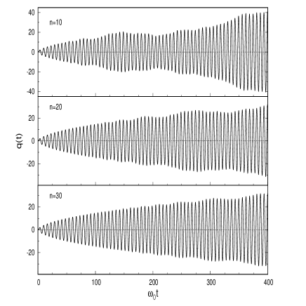
However, the decays of the transient $\varphi(t)$ is slow, and it is getting slower as $\lambda\to\lambda_{c}$. As a result, there is a significant time interval, whose duration increases, in fact diverges, as $\lambda\to\lambda_{c}$, when $\varphi(t)$ oscillates with an almost constant amplitude. Then the solution $q(t)$ is governed by the interplay of two oscillating terms in Eq. (28). As a result, the solution, during a long, albeit finite, time interval, has not a harmonic form (29), but instead shows a beat pattern. For a fixed value of $\lambda$ close to $\lambda_{c}$, the beat period tends to increase when $\Lambda\to 1$. In the limits $\lambda\to\lambda_{c}$ and $\Lambda\to 1$ the initial increasing section of the first beat has the infinite duration, and the solution takes the quasi-resonance form Eq. (18). The tendency is shown in Fig. 1.

VI Response of nonergodic configurations

Consider now the oscillator with natural frequency $\omega>\omega_{c}$. The localized mode now is fully developed, and the Green’s function, according to Eq. (11), involves the harmonic (nonergodic) term $G_{0}\sin\omega_{*}t$. In that case one may anticipate the response to be similar to that of the undamped oscillator with the natural frequency $\omega_{*}$, showing the resonance at $\Omega=\omega_{*}$. The expectation is confirmed by the calculations below.

For nonergodic configurations with $\omega>\omega_{c}$ the Green’s function has now both ergodic and nonergodic (periodic) components, $G(t)=G_{e}(t)+G_{0}\,\sin(\omega_{*}t)$. Substituting this into Eq. (7), taking into account Eq. (12) for $G_{e}(t)$, changing the integration order, and integrating over $\tau$ yields the result for $q(t)$. We write it as

$$q(t)=q_{e}(t)+q_{ne}(t),$$ (30)

where the first and second terms come from the ergodic and nonergodic components of the Green’s function, respectively. The ergodic term $q_{e}(t)$ coincides with the response of the ergodic configuration given by Eq. (28),

$$q_{e}(t)=\frac{F_{0}}{m\omega_{0}^{2}}\Big{\{}A\,\sin(\Omega t-\pi)+\varphi(t)\Big{\}},$$ (31)

where $A$ and $\varphi(t)$ are still given by integral expressions (24) and (25). However, for the given domain $(\lambda>\lambda_{c},\,\Lambda\geq 1)$, expression (24) for $A$ is reduced not to Eq. (27), but to a more involved form

$$A=\frac{2(4\lambda^{2}-1)\left(\Lambda^{2}-\Lambda\sqrt{\Lambda^{2}-1}\right)-4\lambda^{2}}{(4\lambda^{2}-1)(4\lambda^{4}-4\lambda^{2}\Lambda^{2}+\Lambda^{2})}.$$ (32)

At $\Lambda=\Lambda_{0}=4\lambda^{4}/(4\lambda^{2}-1)$ both the numerator and the denominator are zero, and the expression has to be extended by continuity,

$$A(\Lambda_{0})=\lim_{\Lambda\to\Lambda_{0}}A=\frac{1}{2\lambda^{2}\,(4\lambda^{2}-1)\,(2\lambda^{2}-1)}.$$ (33)

One observes that the amplitude $A$ behaves qualitatively similar to that for ergodic configurations, Eq. (27). For any fixed value of $\lambda>\lambda_{c}$ the amplitude $A$ as a function of $\Lambda$ monotonically decreases and shows no maximum (no resonance) near $\Lambda=\lambda$ ($\Omega=\omega$).

The function $\varphi(t)$ in Eq. (31) is still given by Eq. (25). One can verify numerically that for the given domain it is transient, i.e. dies out at long times. However, as for the subcritical case $\lambda\leq\lambda_{c}$, the decay time of $\varphi(t)$ is getting longer and diverges when $\lambda\to\lambda_{c}$ and $\Lambda\to 1$. As a result, the ergodic component $q_{e}(t)$ behaves similar to the solution for ergodic configurations with $\lambda\leq\lambda_{c}$. For $\lambda$ close to $\lambda_{c}$ and $\Lambda$ close to $1$, $q_{e}(t)$ shows on a shorter time scale beats patterns similar to those illustrated in Fig. (1). In the limit $\lambda\to\lambda_{c}^{+}$ and $\Lambda\to 1^{+}$ the duration of the first beat diverges and $q_{e}(t)$ takes the quasi-resonance form (18). For a finite $\lambda-\lambda_{c}>0$, $q_{e}(t)$ evolves on a longer time scale to the steady state solution oscillating with frequency $\Omega$.

Figure 2: The response functions for a nonergodic configuration with $\lambda=0.72$ and $\Lambda=1.005$. Top: the ergodic component $q_{e}(t)$, Eq. (31). Middle: the nonergodic component $q_{ne}(t)$, Eq. (34). Bottom: the total solution, $q(t)=q_{e}(t)+q_{ne}(t)$. The ergodic and nonergodic components oscillate with amplitudes which increase with time as $\sqrt{t}$ and $t$, respectively.

Consider now the the nonergodic term $q_{ne}(t)$ in Eq. (30). Substituting the nonergodic component of the Green’s function $G_{0}\sin\omega_{*}t$ into Eq. (7) yields

$$\!\!\!q_{ne}(t)\!=\!\frac{F_{0}\,G_{0}}{m}\,\frac{1}{\Omega^{2}-\omega_{*}^{2}}\Big{[}\Omega\,\sin(\omega_{*}t)\!-\!\omega_{*}\sin(\Omega\,t)\Big{]},$$ (34)

for $\Omega\neq\omega_{*}$, and

$$q_{ne}(t)=\frac{F_{0}\,G_{0}}{2m}\,\Big{[}\frac{1}{\Omega}\,\sin(\Omega\,t)-t\,\cos(\Omega\,t)\Big{]},$$ (35)

for $\Omega=\omega_{*}$. Those are exactly the expressions for the response of the undamped oscillator with the natural frequency $\omega_{*}$, describing beat patterns for $\Omega\neq\omega_{*}$ and unbounded resonance for $\Omega=\omega_{*}$.

The total response $q(t)=q_{e}(t)+q_{ne}(t)$ is determined by the interplay of both ergodic and nonergodic components and shows a variety of beat patterns for $\Omega\neq\omega_{*}$ and unbounded resonance for $\Omega=\omega_{*}$. Of special interest is the asymptotic case ($\lambda\to\lambda_{c}^{+},\,\Lambda\to 1^{+}$) when both components on a long time scale show the resonance-like behavior, $q_{e}(t)\sim tJ_{0}(\omega t)$ and $q_{ne}(t)\sim t\cos(\omega_{0}t)$. The case is illustrated in Fig. 2.

VII Conclusion

The response properties of an open oscillator with a well-developed localized mode with frequency $\omega_{*}$ are similar to those of an isolated oscillator with the natural frequency $\omega_{*}$. In particular, when the frequency of the external force $\Omega$ coincides with $\omega_{*}$, the oscillator, instead of evolving into a steady state, shows an unbounded resonance. Superficially, this might come as a surprise since the equation of motion (4) involves a dissipation term (which usually smooths out resonance singularities) and also because the equation does not involve the frequency $\omega_{*}$ explicitly. However, from a more educated point of view, which we tried to develop in this paper, the unbounded resonance at $\Omega=\omega_{*}$ is hardly unexpected, considering that the localized mode does not exchange energy with the thermal bath and thus behaves as an isolated oscillator.

Figure 3: Simulation results for the quasi-resonance set up ($\omega=\omega_{c}$, $\Omega=\omega_{0}$) when the bath is represented by a finite harmonic chain of $n=10,20$, and $30$ atoms. As $n$ increases further, the simulation results quickly converges to Eq. (18).

More subtle is the result for the critical value of the oscillator natural frequency $\omega_{c}$ when, according to Eq. (11), the localized mode is incipient. In that case, even though the localized mode does not affect characteristics of the unperturbed system, the dynamical response may have a singular quasi-resonance form (18), which has no analog or counterpart in other open oscillator models. While only a specific dissipation kernel (2) was considered here, one may expect similar results for other kernels whose spectral density has a finite upper bound.

Although the presented results are exact, it might be of interest to verify and extend them with numerical simulations. As we already mentioned, the generalized Langevin equation with the kernel (2) describes a terminal atom of a semi-infinite harmonic chain subjected to an external harmonic potential and driven by an external periodic force. Figure 3 shows the simulation results for the quasi-resonance response of the oscillator coupled to the finite chain of $n$ atoms. The dependence of the response on the size of the thermal bath may be of interest for biochemical applications when both a system and a bath correspond to degrees of freedom of a single macromolecule Chalopin ; Xie1 ; Xie2 . Simulation shows that for $n$ of an order of $100$ or more the quasi-resonance response is practically indistinguishable from the result (18) for the infinite bath. For smaller $n$ the amplitude of oscillations as a function of time is non-monotonic, yet on the long run the response increases with time indefinitely.

We have already noted in Ref. Plyukhin that the parametric transition between ergodic ($\omega\leq\omega_{c}$) and nonergodic ($\omega>\omega_{c}$) configurations resembles a phase transition of the second kind. From that perspective, the quasi-resonance response of the configuration with $\omega=\omega_{c}$ can be viewed as a critical phenomenon, and the exponent $1/2$ in the asymptotic form of Eq. (18), $q(t)\sim t^{1/2}\cos(w_{0}t-\pi/4)$, can be interpreted as a critical exponent.

In this paper we considered the response only at high frequency $\Omega\geq\omega_{0}$. For the low-frequency response at $\Omega<\omega_{0}$, or $\Lambda<1$, the integral expressions (24) and (25) for $A$ and $\varphi(t)$ diverge and are not valid. One can show that the results can be extended for the low-frequency response merely by defining the improper integrals in Eqs. (24) and (25) in the sense of Cauchy principal value. The justification, however, requires a more involved technique and will be addressed in a future publication.

APPENDIX

The integral (17)

$$I(t)=\int_{0}^{t}J_{1}(\tau)\,\sin(t-\tau)\,d\tau$$ (A1)

can be evaluated as follows. The Laplace transform of $J_{1}(t)$ is

$$\tilde{J}_{1}(s)=\mathcal{L}\{J_{1}(t)\}=\frac{1}{s^{2}+s\sqrt{s^{2}+1}+1},$$ (A2)

and the convolution (A1) in the Laplace domain has the form

$$\tilde{I}(s)=\mathcal{L}\{I(t)\}=\frac{1}{(s^{2}+1)(s^{2}+s\sqrt{s^{2}+1}+1)}.$$ (A3)

In terms of partial fractions it can be written as

$$\!\!\!\!\!\!\tilde{I}(s)\!=\!\frac{1}{s^{2}+1}\!-\!\frac{s}{(s^{2}+1)^{3/2}}\!=\!\frac{1}{s^{2}+1}\!+\!\frac{d}{ds}\frac{1}{\sqrt{s^{2}+1}}.$$ (A4)

Then, using the property

$$\mathcal{L}\{t\,f(t)\}=-\frac{d}{ds}\mathcal{L}\{f(t)\}=-\frac{d}{ds}\,\tilde{f}(s)$$ (A5)

and taking account the transform of the Bessel function $\mathcal{L}\{J_{0}(t))=1/\sqrt{s^{2}+1}$, one finds

$$I(t)=\sin(t)-tJ_{0}(t).$$ (A6)

This is Eq. (17) of the main text.

References

- (1) E. W. Montroll and R. B. Potts, Effect of defects on lattice vibrations, Phys. Rev. 100, 525 (1955).
- (2) E. Teramoto and S. Takeno, Time dependent problems of the localized lattice vibration, Prog. Theor. Phys. 24, 1349, 1960.
- (3) S. Kashiwamura, Statistical dynamical behaviors of a one-dimensional lattice with an isotopic impurity, Prog. Theor. Phys. 27, 571, 1962.
- (4) R. Rubin, Momentum autocorrelation functions and energy transport in harmonic crystals containing isotopic defects, Phys. Rev. 131, 964, 1963.
- (5) F. Ishikawa and S. Todo, Localized mode and nonergodicity of a harmonic oscillator chain, Phys. Rev. E 98, 062140 (2018).
- (6) A. V. Plyukhin, Non-Clausius heat transfer: The method of the nonstationary Langevin equation, Phys. Rev. E 102, 052119 (2020).
- (7) G. Kemeny, S. D. Mahanti, and T. A. Kaplan, Generalized Langevin equation for an oscillator, Phys. Rev. B 34, 6288 (1986).
- (8) A. Dhar and K. Wagh, Equilibration problem for the generalized Langevin equation, Europhys. Lett. 79, 60003 (2007).
- (9) A. V. Plyukhin, Nonergodic Brownian oscillator, Phys. Rev. E 105, 014121 (2022).
- (10) R. Morgado, F. A. Oliveira, G. G. Batrouni, and A. Hansen, Relation between anomalous and normal diffusion in systems with memory, Phys. Rev. Lett. 89, 100601 (2002).
- (11) I. V. L. Costa, R. Morgado, M. V. B. T. Lima and F. A. Oliveira, The fluctuation-dissipation theorem fails for fast superdiffusion, Europhys. Lett 63,173 (2003).
- (12) J. D. Bao, P. Hanggi, and Y. Z. Zhuo, Non-Markovian Brownian dynamics and nonergodicity, Phys. Rev. E 72, 061107 (2005).
- (13) L. C. Lapas, R. Mogrado, M. H. Vainstein, J. M. Rubi, and F. A. Oliveira, Khinchin theorem and anomalous diffusion, Phys. Rev. E 101, 230602 (2008).
- (14) W. Deng and E. Barkai, Ergodic properties of fractional Brownian-Langevin motion, Phys. Rev. E 79, 011112 (2009).
- (15) P. Siegle, I. Goychuk, P. Talkner, and P. Hanggi, Markovian embedding of non-Markovian superdiffusion, Phys. Rev. E 81, 011136 (2010).
- (16) Y. Chalopin and J. Sparfel, Energy bilocalization effect and the emergence of molecular functions in proteins, Front. Mol. Biosci. 8, 736376 (2021).
- (17) R. Zwanzig, Nonequilibrium Statistical Mechanics, Oxford University Press, NY (2001).
- (18) U. Weiss, Quantum Dissipative Systems, World Scientific, Singapore (2008).
- (19) S. C. Kou and X. S. Xie, Generalized Langevin equation with fractional Gaussian noise: Subdiffusion within a single protein molecule, Phys. Rev. Lett. 93, 180603 (2004).
- (20) W. Min, G. Luo, B. J. Cherayil, S. C. Kou, and X. S. Xie, Observation of a power-law memory kernel for fluctuations within a single protein molecule, Phys. Rev. Lett. 94, 198302 (2005).
- (21) I. Goychuk, Viscoelastic subdiffusion: Generalized Langevin equation approach, Adv. Chem. Phys. 150, 187 (2012).
- (22) S. Burov and E. Barkai, Critical exponent of the fractional Langevin equation, Phys. Rev. Lett. 100, 070601 (2008).
- (23) S. Burov and E. Barkai, Fractional Langevin equation: Overdamped, underdamped and critical behaviors, Phys. Rev. E 78, 031112 (2008).
- (24) G. N. Watson, A Treatise on the Theory of Bessel Functions, second ed., Cambridge University Press, London, 1944, section 12.21.
- (25) W. N. Bailey, Some integrals of Kapteyn’s type involving Bessel functions, Proc. London Math. Soc., s2-30, 422, (1930).