Designing Fair, Cost-optimal Auctions based on Deep Learning for Procuring Agricultural Inputs through Farmer Collectives

Abstract

Procuring agricultural inputs (agri-inputs for short) such as seeds, fertilizers, and pesticides, at desired quality levels and at affordable cost, forms a critical component of agricultural input operations. This is a particularly challenging problem being faced by small and marginal farmers in any emerging economy. Farmer collectives (FCs), which are cooperative societies of farmers, offer an excellent prospect for enabling cost-effective procurement of inputs with assured quality to the farmers. In this paper, our objective is to design sound, explainable mechanisms by which an FC will be able to procure agri-inputs in bulk and distribute the inputs procured to the individual farmers who are members of the FC. In the methodology proposed here, an FC engages qualified suppliers in a competitive, volume discount procurement auction in which the suppliers specify price discounts based on volumes supplied. The desiderata of properties for such an auction include: minimization of the total cost of procurement; incentive compatibility; individual rationality; fairness; and other business constraints. An auction satisfying all these properties is analytically infeasible and a key contribution of this paper is to develop a deep learning based approach to design such an auction. We use two realistic, stylized case studies from chili seeds procurement and a popular pesticide procurement to demonstrate the efficacy of these auctions.

1 Introduction

Sourcing the right quality and quantity of agricultural inputs (agri-inputs for short) such as seeds, fertilizers, pesticides, farm equipment, and human resources is a critical aspect of agricultural operations. This is a universal problem faced by farmers throughout the globe and especially in emerging economies.

Agri-Inputs: In order to maximize yield, it is necessary for farmers to use the right quantities of right quality inputs. Agricultural inputs are external inputs required to help the various farming operations. They range from high-quality seeds, fertilizers, pesticides, to high-tech tractors and farm equipment. There are mainly two categories of agri-inputs: consumable and capital. Consumable inputs are used commonly and regularly by the farmers - seeds, fertilizers, pesticides, etc. These are essentially natural materials that will be consumed by the crops. Capital inputs include farm equipment such as tractors, agricultural robots, trellising materials, etc. In addition to all these, we have human labor. In this paper, we focus on consumable inputs.

Seeds that are usually procured include: vegetables, cotton, paddy, maize, sorghum, sunflower, wheat, millets, mustard, chili peppers, and lentils. High quality seeds facilitate smooth farming; low quality seeds can lead to crop losses and even crop destruction. Pesticides used by farmers belong to the following categories: (a) herbicides, (b) insecticides, (c) fungicides, (d) nematicides, and (e) rodenticides. The use of pesticides in right quantities at the right time saves the crops from being destroyed. Fertilizers are any materials of natural or synthetic origin that are applied to soil or to plant tissues to supply plant nutrients.

The Context and Need: In many emerging economies, most of the farmers are small or marginal, holding less than 5 acres of land. Their economic condition is weak and they mostly depend on credit for sustaining their operations. The farmers are faced with a dilemma at the start of every cropping season over where to procure agri-inputs from. Most of these farmers, being small, buy the inputs on credit. It is extremely important for them to get quality inputs, but, often, they end up with low quality inputs leading to crop losses or even crop failures. To quote a typical farmer in one of the emerging economies: “If inputs are substandard or fake, we have to go through a minimum of two years of suffering due to debt. Therefore, in addition to the good rains, the quality of inputs we buy decides our farm income season after season." In fact, approximately 50 percent of the total cost goes towards inputs [1].

A seemingly simple and promising way in which this problem could be solved is to create economies of scale in procuring high quality inputs through a collective action by setting up a bulk procurement system. Bulk procurement also makes it easier to ensure that the quality of input is maintained. In many countries, the respective governments have taken up the initiative to launch farmer collectives or farmer cooperatives (FCs) to help out the small and marginal farmers in various input and output operations. In particular, FCs would be extremely helpful for reducing the input burden on the farmer through bulk procurement of inputs, after collecting information on the input requirements of individual farmers (this could be done, for example, by a well designed mobile app to reach out to all farmer members of the FC). This paper specifically focuses on this problem and explores the use of systematic methods for harnessing the bargaining power of farmer collectives.

There exist more than 1500 FCs in Brazil, more than 7500 FCs in Germany, more than 63000 FCs in India, and more than 1700 FCs in USA. A recent report [2] mentions a staggering 1.2 million agricultural cooperatives across the globe today. It may not be unreasonable to expect a saving of US $ 100 for procuring a typical seed variety in a typical FC which may consist of a few hundreds of farmers. Thus, such collective action for agri-input procurement has the potential for huge impact.

To gain a first-hand experience and knowledge of the real situation on the ground, our research group undertook a field study of two FCs, Anekal Horticulture Producers Company Limited and Rajaghatta Horticulture Farmer Producer Company Limited, both within 50 km from Bengaluru, India. Both FCs have a membership of about 1000 farmers each. Small and marginal farmers tend to be low on education and are particularly vulnerable to the strategic tactics of intermediaries. Since the intermediaries offer credit to the farmers for sourcing the inputs, the intermediaries are able to wield their influence in the marketing and selling of the produce as well. In the process, the farmers end up on the losing side. The FCs play a key role in streamlining the supply of inputs to the farmers and can counter the selfish moves of the intermediaries. Our team had a detailed discussion with the FCs on how they collect indents, aggregate the input requirements of the farmers and bulk-procure the right quantities of inputs to be sold subsequently to the farmers at affordable prices. During these conversations, we also realized numerous issues which were hampering a successful execution of the bulk procurement process. For example, FCs do need a healthy amount of money and resources to execute this process more efficiently. We also discussed with the FCs the discounts that they would be able to obtain because of both volume and variety of their purchases. Here again, we found that the discounts on offer from the suppliers could be much higher if the right kind of procurement mechanisms are put in place.

Note that there are numerous types and varieties of seeds. There are numerous types of pesticides and fertilizers. The total savings, by conservative estimates, easily runs into Billions of Dollars (a more methodical and accurate estimate of this is beyond the scope of this paper). Above all, the farmers, who are often naive, are insulated from the transactions and further, the quality levels of agri-inputs are assured.

Since scientifically designed auction mechanisms can promote honest behavior and healthy competition among suppliers [3], we propose to develop a suitable procurement auction (also called reverse auction) mechanism for bulk procurement of agri-inputs by FCs.

Procurement Auctions for Bulk Procurement by Farmer Collectives: We explain the workflow of the proposed agri-input procurement with an example. Let us consider procurement of paddy seeds. Suppose the farmer collective has 1000 farmer members (like Anekal or Rajghatta described above) who want to grow paddy and suppose there are five varieties of paddy seeds. The FC will collect from the farmers (this can be done using a mobile app), the quantum and type of seeds required by each farmer. The FC will aggregate these requirements into five buckets, each bucket corresponding to a particular seed variety. Each bucket will then correspond to a certain large volume of seeds of that variety needed by all the farmers. For each bucket, the FC will identify suppliers for the seeds, qualify them based on the reputation and quality standards, and conduct an auction involving the qualified suppliers.

First, we bring out the most desirable properties for such an auction mechanism. Our analysis is based on our familiarity with and study of FCs and agri-input procurement.

1. Incentive compatibility (IC)
   Incentive compatibility ensures truthful bidding by the suppliers and is a fundamental requirement of any auction mechanism. The most powerful version of IC is dominant strategy incentive compatibility (DSIC), which means bidding true values is best irrespective of the bids of the other players.

2. Individual rationality (IR)
   Individual rationality ensures that the suppliers obtain non-negative utility by participating in the auction. The most powerful version of IR is ex-post IR, which implies that the utility to each participating player will be non-negative irrespective of the bids of the other players.

3. Social welfare maximization (SWM)
   This implies maximizing the sum of utilities of the participants in the auction. In a procurement auction, the participants involved are the FC and the suppliers.

4. Cost minimization (OPT)
   This means the expected total cost of procurement is minimized by the auction. Cost minimization is a key requirement since we wish to minimize the input costs to the small and marginal farmers.

5. Fairness (FAIR)
   Fairness implies that the winning suppliers are chosen in a fair way. An index of fairness would be envy-freeness – no supplier can increase her utility by adopting another supplier’s outcome. If envy-freeness is not achievable, the next best option is envy minimization (which is what we pursue in this paper).

6. Business constraints (BUS)
   Satisfaction of business constraints refers to constraints such as having a minimum number of winning suppliers (to avoid monopoly), a maximum number of winning suppliers (to minimize logistics costs), a maximum fraction of business to be awarded to any supplier, etc.

Further, the auction should extract volume discounts or quantity discounts from suppliers. This final requirement points to using auctions where the suppliers can specify volume discounts as a part of their bids.

Volume discount auctions or quantity discount auctions, which are very relevant to this work are covered in [4, 5, 6, 7, 8]. In a volume discount auction, the buyer wishes to procure a large volume of a certain item type and the suppliers announce supply curves or volume discount bids. A supply curve specifies the discounted prices offered by the supplier.

Example 1: Suppose we are procuring paddy seeds in packets (usually a packet may correspond to a certain number of kilograms). Let an example supply curve be ((1-500: 20), (501-1500: 18), (1501-2500: 16)). This would mean: the supplier offers a per unit price of $20 when the quantity is in the range 1-500; a per unit price of $18 when the quantity is in the range 501-1500; and a per unit price of $16 when the quantity is in the range 1501-2500. If the seller is supplying 1800 units, the total bid price will be $500\times\$20+1000\times\$18+300\times\$16=\$32800$. Our field studies have shown that such supply curves are quite common in bulk procurement of agri-inputs. In this paper, we are concerned with design of such auctions.

Contributions and Outline: A recent paper [9] has addressed the problem of procuring agri-inputs through farmer collectives by proposing volume discount auctions and combinatorial auctions. [9] proposes Vickrey-Clarke-Groves (VCG) payments to ensure that the auction is dominant strategy incentive compatible and maximizes social welfare. Their auction also takes into account certain business constraints such as minimum number of winning suppliers and maximum number of winning suppliers. Their auction is based on the methods described in [4, 5, 6, 7, 8] and performs better than the naive methods which are currently being used. However, their auction crucially does not minimize the total cost of procurement and does not implement any notion of fairness.

Satisfying all of the six properties listed above (IC, IR, SWM, OPT, FAIR, BUS) is clearly a tall order. Mechanism design theory [10, 11] is replete with impossibility theorems which make it clear that these properties cannot be simultaneously satisfied. The ambitious goal of this paper is to innovatively devise auctions that achieve maximal subsets of these objectives with as little compromise as possible.

The methodology proposed in this paper hinges on our technically novel extension to a recent line of research [12, 13, 14] that explores a deep learning approach to optimal auction design and achieves, in the sense of regret minimization, properties IC, IR, and OPT. Our methodology considers volume discount bids and achieves, properties FAIR and BUS in addition, with a slight compromise in SWM. This is a key technical contribution of this paper, which is described in the next section (Section 2).

The design of the auction mechanism above is clearly motivated by the agri-input procurement by farmer collectives. We demonstrate the efficacy of these mechanisms through thought experiments in Sections 3 and 4. In Section 3, we conduct experiments on data that are synthetically generated based on real-world observations of the volume discounts offered by different suppliers. In Section 4, we describe two realistic, stylized case studies: (1) procurement of chili pepper seeds (2) procurement of a popular, commonly used pesticide. We describe our experiments on these case studies; the results again highlight the superior performance of the proposed mechanism. Finally, Section 5 concludes the paper and provides some directions for future work.

2 A Deep Learning Approach for Volume Discount Procurement Auctions

As stated already, a volume discount auction satisfying DSIC, IR, OPT, FAIR, and BUS is impossible in mechanism design [10, 11]. To surmount this, we adopt a deep learning approach, which solves this design problem as a regret minimization problem on the lines of [13]. Even though our architecture resembles the RegretNet architecture proposed by [13], it is notable that the RegretNet architecture cannot be applied as an off-the-shelf mechanism for volume discount procurement auctions. There are two technical reasons for this.

The first reason has to do with satisfying individual rationality. RegretNet is designed for forward auctions (selling scenario) while the procurement auction is a reverse auction. IR requires that all agents receive a higher utility by participating in the auction than by not participating. In a forward auction, this means that no buyer should be paying more than their valuation of the items allocated to them. In a procurement auction, on the other hand, this means that no seller would accept a payment lower than their valuation for the items they are selling. For the procurement auction setting, the network requires a subtle modification (see Section 2.3) to satisfy the IR condition.

The second reason is more fundamental. We are dealing with the procurement of homogeneous units with volume discounts whereas the work of [13] considers auctions with additive (or unit-demand) valuations. Our volume discount auction setting is not additive and is not unit-demand either. To see this, observe that the value of $2x$ units with volume discounts is not the same as twice the value of $x$ units. Additionally, the suppliers in our setting wish to sell any number of units, unlike the unit-demand buyers considered by [13]. Auctions with additive valuations and unit-supply valuations make it possible to use allocation networks whose outputs are simply (stochastic) allocation matrices. We simply cannot do this in our case, so instead, we produce an allocation tuple as output - with each element in the tuple being the allocation for the corresponding supplier. This complicates the computation of the payments and makes theoretical analysis significantly complex.

2.1 The Volume Discount Procurement Auction Setting

In this section, we formally describe the volume discount auction setting. There is a single buyer who intends to procure $m$ homogeneous units of a certain item from $n$ suppliers using a procurement auction with volume discount bids. Let $\ell:=\lfloor\frac{m}{k}\rfloor$ for some predefined $k$. The volume discount bidding is implemented as follows. First, each supplier $i$ submits a volume discount bid in the form of a vector $b^{(i)}=(b^{(i)}_{1},b^{(i)}_{2},\cdots,b^{(i)}_{k})$ of $k$ intervals (See Remarks subsection below for details). Then, given the vector of bids $b=(b^{(1)},\cdots,b^{(n)})$ as input, the procurement mechanism outputs allocation and payment vectors denoted by the tuple $\langle a(b),p(b)\rangle$. Here, $a(b)=(a_{1}(b),\cdots,a_{n}(b))$ denotes the allocation vector and $p(b)=(p_{1}(b),\cdots,p_{n}(b))$ denotes the payment vector with each $a_{i}(b)$ being the number of units bought from supplier $i$ and $p_{i}(b)$ being the payment made to supplier $i$. Note that such auctions or variants have been considered earlier in [4, 5, 6, 7, 8]. In this paper we seek nontrivial extensions, to satisfy additional properties such as FAIR and BUS.

The suppliers have their own private willingness to sell (WTS), which determines the minimum price at which the supplier is ready to sell. For supplier $i$, denote the WTS by $v^{(i)}=(v^{(i)}_{1},...,v^{(i)}_{k})$. These valuations are assumed to be drawn from some prior distribution $\mathcal{F}$. In our setting, $\mathcal{F}$ is common knowledge among all the suppliers and the buyer, whereas the realized vector of valuations $v^{(i)}$ is known privately only to the individual supplier $i$.

The utility for a supplier is defined as a function of her private valuations $v^{(i)}$, allocation $a$, and payment $p$, and is given by

$$u_{i}(v^{(i)};b)=p_{i}(b)-\sum_{j=1}^{a_{i}(b)}v^{(i)}_{\lceil j/\ell\rceil}$$ (1)

We now recall some definitions. A mechanism is DSIC if no agent can gain utility by misrepresenting its valuations, regardless of the strategies adopted by the other agents. That is,

$$u_{i}(v^{(i)};(v^{(i)},b^{(-i)}))\geq u_{i}(v^{(i)};b)\qquad\forall v,b,i.$$ (2)

An auction mechanism is called ex-post IR if every agent earns non-negative utility by participating in the auction. We assume that there is no participation/entry cost. Our proposed neural network architecture is designed to ensure the ex-post IR condition which is equivalent to

$$u_{i}(v^{(i)};v)\geq 0\qquad\forall v,i.$$ (3)

The goal is to minimize the cost incurred by the buyer, subject to DSIC and ex-post IR for the sellers. The total cost to the buyer is given by

$${\tt cost}=\sum_{i=1}^{n}p_{i}(b).$$ (4)

We remark here that the cost minimization under DSIC and IR constraints corresponds to a nontrivial extension of the celebrated revenue optimal auction theory [15] (Myerson’s auction only considers a single item and a weaker form of incentive compatibility, namely Bayesian incentive compatibility). Our approach considers additional, practically motivated constraints (multiple units, volume discount bids, envy minimization, and business constraints). Following section 2.2.2 of [13], one can guarantee DSIC property by ensuring that the expected ex-post regret for every supplier, $r_{i}$, is $0$. The expected ex-post regret of a procurement mechanism is defined as

$$r_{i}=\mathbb{E}_{v\sim\mathcal{F}}[\max_{b}[u_{i}(v^{(i)};b)-u_{i}(v^{(i)};(v^{(i)},b^{(-i)}))]].$$ (5)

The regret is computed empirically, which adequately approximates the real regret [13].

Remarks:

• The mechanism solicits volume discount bids from each supplier. These bids represent each agent’s valuation for a single unit from each ‘lot’ of units. There are $k$ lots of (almost) equal size. The supplier $i$’s bid $b_{1}^{(i)}$ is applied to all the goods if the buyer procures at most one lot; i.e. $\ell$ goods. For the goods from the second lot, the bid $b_{2}^{(i)}$ is used, i.e., a price of $b_{1}^{(i)}$ per unit for the first $\ell$ goods and a price of $b_{2}^{(i)}$ for the remaining goods (up to $\ell$). And so on.

• All the goods from a given lot are valued equally. Thus, if the supplier sources more lots, her valuation per good decreases. In the agricultural domain, this corresponds to savings from the use of bulk transport, warehouse clearance, mass production, etc.

• In many practical settings, the value of $k$ is determined endogenously. This value depends on factors such as packaging method, carton size, nature of the goods, etc. However, when $k$ is a design parameter, it presents an interesting challenge in auction design. A larger value of $k$ introduces more granularity, which is better for the buyer. But it also introduces complex bidding procedures possibly leading to a less effective implementation. We leave the study of this aspect as an interesting future work.

Example 2: Recall Example 1 where we had the supply curve: ((1-500: 20), (501-1500: 18), (1501-2500: 16)). Here $m=2500$. Suppose $k=5$. We will have $\ell=500$. The intervals would be $[1,500]$, $[501,1000]$, $[1001,1500]$, $[1501,2000]$, $[2001,2500]$. Let the first supplier’s WTS be $v^{(1)}=(20,18,18,16,16)$. If $1800$ items are acquired from the first supplier, the supplier’s WTS for the allocation would be $500\times 20+500\times 18+500\times 18+300\times 16=32800$. Now assume that the second supplier has a production capacity of $1500$ units, and she offers a fixed volume discount after $500$ units. That is, $v^{(2)}=(18,17,17,\infty,\infty)$. If the allocation for the second supplier is $700$ units, then her WTS for the allocation is $500\times 18+200\times 17=12400$. Thus, the suppliers may have a wide variety of different supply curves and still fit within the setting considered in this paper.

2.2 Deep Learning Based Formulation

We propose a neural network based formulation to obtain DSIC and IR guarantees along with some other desirable and practical constraints. The goal is to minimize a composite loss function that consists of the following three parts. The objective cost (i.e., the total payment), the regret penalty, and the Lagrangian term (as we use the method of differential multipliers [16]) for regret. In particular, we have

$\displaystyle{\tt loss}={\tt cost}+{\tt penalty_{regret}}$ $\displaystyle+{\tt LagrangianLoss}$ $\displaystyle{\tt cost}$ $\displaystyle=\sum_{i=1}^{n}p_{i}(b)$ $\displaystyle{\tt LagrangianLoss}$ $\displaystyle=\sum_{i=1}^{n}\lambda_{{\tt regret}}^{(i)}\tilde{r}_{i}$ $\displaystyle{\tt penalty_{regret}}$ $\displaystyle=\rho_{{\tt regret}}\sum_{i=1}^{n}\tilde{r}_{i}^{2}$

Here, $\tilde{r_{i}}$ is the empirical regret. We compute $\tilde{r_{i}}$ by using another optimizer over the bids, coming from the same distribution as $\mathcal{F}$, which maximizes the utility for agent $i$. To approximate the expectation over the distribution $\mathcal{F}$, we maximize the sample mean of regret over the batch. We discuss more on this subsequently.

2.2.1 Business Constraints

The buyer may wish to impose various business constraints in the procurement auction - for example, the buyer may require that at least 3 suppliers supply at least $20\%$ of the items each. We take care of this by adding a penalty term for violating various business constraints while training the network. For having a minimum of $s$ suppliers each with an allocation of at least $a_{min}$, the penalty would be

$${\tt penalty_{business}}=\begin{cases}0&a^{(s)}\geq a_{min}\\ \frac{\rho_{{\tt business}}}{a^{(s)}}&a^{(s)}<a_{min}\end{cases}$$ (6)

where $a^{(s)}$ is the $s^{th}$-highest allocation. Other business constraints are also possible. For instance, no supplier is allocated more than $50\%$ of the units. The loss function in this case also adds the penalty for violating business constraints.

2.2.2 Envy Minimization

In auctions, it is often desirable to have some additional fairness constraints, specifically, minimization of envy. Envy (or dissatisfaction) for an agent is defined as the maximum utility they could gain if they were given the allocation and payment of some other agent. So the envy for supplier $i$, given the valuation tuple $v=(v^{(1)},...,v^{(n)})$ is

$$e_{i}(v)=\max_{h\in[n]} [(p_{h}(b)-\sum_{j=1}^{a_{h}(b)}v^{(i)}_{\lceil j/\ell\rceil})]-u_{i}(v^{(i)};v)$$ (7)

We minimize envy by adding a term for envy in our Lagrangian loss, along with an envy penalty.

$\displaystyle{\tt loss}={\tt cost}+{\tt penalty_{regret}}$ $\displaystyle+{\tt penalty_{envy}}+{\tt LagrangianLoss}$ $\displaystyle{\tt cost}$ $\displaystyle=\sum_{i=1}^{n}p_{i}(b)$ $\displaystyle{\tt LagrangianLoss}$ $\displaystyle=\sum_{i=1}^{n}\lambda_{{\tt regret}}^{(i)}\tilde{r}_{i}+\lambda_{{\tt envy}}^{(i)}e_{i}$ $\displaystyle{\tt penalty_{regret}}$ $\displaystyle=\rho_{{\tt regret}}\sum_{i=1}^{n}\tilde{r}_{i}^{2}$ $\displaystyle{\tt penalty_{envy}}$ $\displaystyle=\rho_{{\tt envy}}\sum_{i=1}^{n}e_{i}^{2}$

2.2.3 Business Constraints With Envy Minimization

If we wish to have business constraints while simultaneously minimizing envy, the loss function for the network is

$\displaystyle{\tt loss\ =\ cost\ }{\tt+\ penalty_{regret}\ }$ $\displaystyle{\tt\ +\ penalty_{envy}}+{\tt penalty_{business}}+{\tt LagrangianLoss}$ $\displaystyle{\tt cost}$ $\displaystyle=\sum_{i=1}^{n}p_{i}(b)$ $\displaystyle{\tt LagrangianLoss}$ $\displaystyle=\sum_{i=1}^{n}\lambda_{{\tt regret}}^{(i)}\tilde{r}_{i}+\lambda_{{\tt envy}}^{(i)}e_{i}$ $\displaystyle{\tt penalty_{regret}}$ $\displaystyle=\rho_{{\tt regret}}\sum_{i=1}^{n}\tilde{r}_{i}^{2}$ $\displaystyle{\tt penalty_{envy}}$ $\displaystyle=\rho_{{\tt envy}}\sum_{i=1}^{n}e_{i}^{2}$ $\displaystyle{\tt penalty_{business}}$ $\displaystyle=\begin{cases}0&a^{(s)}\geq a_{min}\\ \frac{\rho_{{\tt business}}}{a^{(s)}}&a^{(s)}<a_{min}\end{cases}$

2.3 Allocation Network and Payment Network

The model consists of two feed-forward networks - an allocation network and a payment network (See Fig.  1, Fig. 2 for details). The input for both networks is the $n\times k$ matrix where the $i^{th}$ row is the bid $b^{(i)}$ for supplier $i$, which is assumed to be equal to the valuation. The output of the allocation network is the allocation tuple described in Section 2.1. The allocation network uses soft-max to ensure that the allocation tuple is a probability vector. This is multiplied by $m$ to ensure that the allocations across the agents sum up to exactly $m$. The output of the payment network is a payment multiplier tuple, $\hat{p}=(\hat{p}_{1},...,\hat{p}_{n})$, which, when multiplied by the total WTS of the allocation, gives the payment tuple, i.e.,

$$p_{i}(b)=\hat{p}_{i}(b)\sum_{j=1}^{a_{i}(b)}v^{(i)}_{\lceil j/\ell\rceil}$$ (8)

Each $\hat{p}_{i}$ is guaranteed to be within the range $[1,\infty)$ in order to ensure IR. The network architecture ensures this by using a sigmoid layer followed by the addition of the constant $1$, thus constraining the output to $(1,2)$.

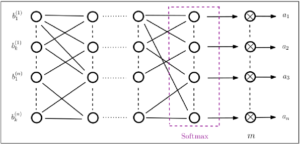
Figure 1: Allocation Network

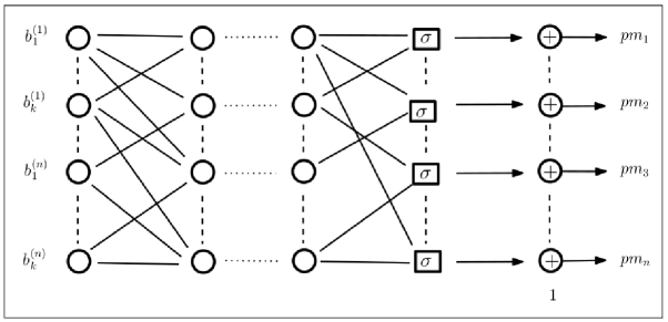
Figure 2: Payment Network

2.4 Training Procedure

In all our experiments, $4$ or $5$ layers, with $60$ to $150$ neurons in each layer, were used for both the payment and allocation networks. The Adam optimizer was used for training the network weights, while stochastic gradient descent was used to learn the Lagrangian parameters and compute the empirical regret.

During the training phase, we performed nested optimizations. For one step of optimization over the network weights, we executed $R$ steps of optimization over the bids, to compute the empirical regret. We did gradient ascent over the Lagrangian parameters after every 2-4 epochs with gradual increase in learning rate over the epochs. This was done to ensure that, first, the network weights converge towards minimizing the cost objective and then, the learned weights get projected in the constrained region to satisfy other required properties of the auction. The above idea for empirical regret computation is the same as the one proposed in [13].

2.5 Some Notes on the Methodology

Versatility: The methodology presented in this paper is versatile in the sense of its ability to model the minimization or maximization of a wide variety of performance metrics. For example, we can use this methodology to maximize the Nash social welfare subject to incentive compatibility, individual rationality, and business constraints. Nash social welfare maximization is widely known for its fairness properties [17]. The techniques presented in [4, 5, 6, 7, 8] correspond to very specific settings and are not generalizable. The approach presented here offers many powerful features that can be modeled in volume discount auctions.

Computational Complexity: The methodology proposed here essentially transforms a mechanism design problem into an optimization problem. So the question would arise as to why an efficient optimization procedure cannot be used to solve the problem, at least approximately. The constraints we deal with such as business constraints and envy minimization are nonlinear and linear approximations do not work well with such constraints. Moreover, the linear approximation will have an exponential number of variables. The deep learning technique has the advantage that a single substantial effort of training will amortize the computational complexity over a large number of experiments.

3 Experimental Results

In this section, we present experimental results for the following six auctions. Notably, all these auctions satisfy DSIC and IR.

1. A standard VCG auction (satisfies SWM)

2. A VCG auction subject to a limit on the minimum number of winning suppliers (satisfies SWM and BUS)

3. A cost minimizing volume discount auction (satisfies OPT)

4. A cost minimizing volume discount auction with envy minimizing allocation (satisfies OPT and FAIR)

5. A cost minimizing volume discount auction with a limit on the minimum number of winning suppliers (satisfies OPT and BUS)

6. A cost minimizing volume discount auction with envy minimizing allocation and with a limit on the minimum number of suppliers (satisfies OPT, FAIR, and BUS)

In this experiment, we have $5$ suppliers. $5$ is a realistic number in agri-settings. In a high volume agri-input procurement, the number of qualified suppliers is typically small. Also, an initial qualification process can be used to weed out suppliers who do not satisfy the quality requirement. This is a definite advantage of bulk procurement; since the FC negotiates the quality and cost, a desired quality and a competitive price are assured. Left to themselves, individual farmers have no bargaining power on either quality or price.

In the current experiment, we assume $5000$ or $10000$ units procured from the suppliers who submit volume discount bids. Each bid will have a set of intervals and a certain discount corresponding to that interval. We use a minimum interval size of $500$ and each interval in a bid has a size that is an integer multiple of the minimum interval size. We assume a base price of US $ $5$ per unit, and a minimum profit margin that ranges from $10\%$ to $30\%$. Recall that the base price plus the minimum profit margin is the willingness to sell of the supplier. The volume discounts typically range from $1\%$ at the first discounted interval to as high as $25\%$ on the highest discounted interval. The data were synthetically generated based on our experience with the field visits we had undertaken to two FCs. For business constraints, we assume at least $3$ winning suppliers have to be selected for procurement. This helps introduce redundancy for decreasing fragility in the supply chain.

Table 1 shows the total procurement cost with six different auctions. We ran the simulation for over 12000 instances, randomly generated from the same distribution as of the training data, and averaged the results to populate the table. We dynamically generate these data to ensure that the model has never seen these data during training. This shows that our model generalizes over the data distribution rather than just over-fitting a particular set of instances.

	Auction Type	5000 Units	10000 Units
1	VCG Auction	$27935$	$52930$
2	VCG Auction + Business Constraints	$30550$	$60100$
3	Cost Minimizing	$27550$	$51950$
4	Cost Minimizing + Envy Minimizing	$27700$	$52350$
5	Cost Minimizing + Business Constraints	$29050$	$56800$
6	Cost Minimizing + Envy Minimizing + Business Constraints	$29600$	$54050$

Table 1: Total procurement cost in US $

Clearly, Auction (6) is the most desirable. It has a cost higher than that of a VCG auction but lower than that of a VCG auction with a limit on the number of winning suppliers. Auction (6) clearly will have a cost lower than that of a VCG auction with envy minimization and limited number of winning suppliers. As expected, Auction (3) (cost minimizing) has the least cost. If envy minimization and business constraints are not a consideration, we go for Auction (3). If envy minimization is important but not business constraints, we go for Auction (4). If business constraints are important but envy minimization can be ignored, we go for Auction (5). If all properties are important, we go for Auction (6). The deep learning based methodology thus enables different options to be exercised based on the context. The key direct benefit is reduction of cost to farmers and the key indirect benefit is assurance of minimum quality.

4 Two Case Studies: Chili Pepper Seeds and a Popular Pesticide

In a typical farmer collective the farmers usually approach intermediaries for sourcing their inputs. The intermediaries allure the farmers by providing credit for sourcing the agri-inputs. In the process, the intermediaries are able to capture the marketing and selling of the produce as well, with huge commissions, causing severe loss of revenue to the farmers. Small and marginal farmers tend to be low on education and are particularly vulnerable to the selfish moves of the intermediaries. This is where the FCs can help; the FCs can play a key role in streamlining the supply of inputs to the farmers and counter the intermediaries.

4.1 Procurement of Chili Pepper Seeds

Our first case study is on chili pepper. This is inspired by the study presented in [9]. There are numerous varieties of chili pepper seeds (more than 50). We consider here two types of seeds (A and B). The seeds come in packets of 4 kg each. There is a demand of 2000 packets for seeds of type A while there is a demand of 1000 packets for seeds of type B. Call each packet a unit. The FC can bulk-procure this requirement from major suppliers of these seeds and then distribute the required volume of seeds to farmers at affordable prices.

We consider a volume discount auction where each volume discount bid has four equal segments offering 2.5%, 5%, 7.5%, and 10% discount on per unit price. For example, in the case of seeds of type A, the 2000 units are divided into four segments, namely, [1,500], [501,1000], [1001, 1500], and [1501, 2000] and in these segments, the discounts offered are 2.5%, 5%, 7.5%, and 10%, respectively of the bid amount when discounts are not offered.

Table 2 presents the results for all six types of auctions separately for type A seeds and type B seeds. These results are computed as averages over 12800 samples with bid amounts drawn from a uniform distribution around the respective base values for different parameters. These results are computed using a trained model, but on data generated separately from the data used for training the model. In all cases, the interval size, $l$, was fixed to be $100$. The base prices for A and B are $17.11 and $14.47 respectively. The minimum profit margin (in %) was assumed to be distributed uniformly over $[8,12]$. Here, we assume there are 10 suppliers.

	Auction Type	2000 A	1000 B
1	VCG Auction	$34880$	$14750$
2	VCG Auction + Business Constraints	$36000$	$15220$
3	Cost Minimizing	$34760$	$14700$
4	Cost Minimizing + Envy Minimizing	$34960$	$14775$
5	Cost Minimizing + Business Constraints	$34770$	$14710$
6	Cost Minimizing + Envy Minimizing + Business Constraints	$35225$	$14960$

Table 2: Chili Pepper seeds: Total procurement cost in US $

From Table 2, it is clear that Auction (6) is the most desirable. In the current context of chili pepper seeds, envy minimization and business constraints are both important and we go for Auction (6). Note that this is an auction that (nearly optimally) satisfies dominant strategy incentive compatibility, ex-post individual rationality, envy minimization, business constraint of minimum number of winning suppliers, and cost minimization. The deep learning based methodology thus enables the best option to be exercised, with the direct benefit of reduction of cost to farmers and the indirect benefit of assured quality of chili pepper seeds.

4.2 Pesticide Procurement

For our experimentation, we have chosen a popular pesticide.This pesticide comes in packets of 250 grams. A typical small farmer may need several packets of pesticides (say 5 to 10). We assume 1000 farmers in the FC and a requirement of 5000 packets to be sourced from 5 suppliers who offer volume discounts. Let $S1$, $S2$, $S3$, $S4$, and $S5$ be the five suppliers. The following are the supply curves of these suppliers.

S1: [1-500; 2.75];[501-1000; 2.69];[1001-2000; 2.62];[2001-3000; 2.56]
S2: [1-100; 3.02];[101-300; 2.94];[301-700; 2.87];[701-1000; 2.81];
    [1001-1400: 2.77];[1401-1800; 2.75];[1801-2200: 2.72];[2201-3000; 2.69]
S3: [1-500: 3.30];[501-1500; 2.87];[1501-3000: 2.81];[3001-4000; 2.77]
S4: [1-500: 3.74];[501-1000; 3.25];[1001-2000; 3.00];[2001-4000; 2.87]
S5: [1-5000; 3.00]

These supply curves have been formulated after conversations with a few pesticide suppliers. The results given are computed using a trained model specifically tuned for this task.

We also provide some additional information for Auction (3). The same for the other auctions is omitted for the sake of brevity. The model provided an allocation of $[2937,1980,83,0,0]$ and a payment of $[8299,5731,274,0,0]$ for the 5 suppliers (in order). The total payment is thus $14304$ (rounded to $14300$). This is in contrast to Auction (1) where the allocation is $[3000,2000,0,0,0]$ and the payment is $[8626,5931,0,0,0]$ for the 5 suppliers (in order). Thus, total payment for VCG is $14557$ (rounded to $14560$).

Table 3 presents the results for all six types of auctions. The trends exhibited are identical to the case of chili pepper seeds. Here again, envy minimization and business constraints are both important and we go for Auction (6). The deep learning based methodology thus enables the best option to be exercised, with the direct benefit of reduction of cost to farmers and the indirect benefit of assured quality of pesticide procured.

	Auction Type	Cost (in US $)
1	VCG Auction	$14560$
2	VCG Auction + Business Constraints	$14710$
3	Cost-Minimizing	$14300$
4	Cost-Minimizing + Envy-Minimization	$14490$
5	Cost-Minimizing + Business Constraints	$14390$
6	Cost-Minimizing + Envy-Minimization + Business Constraints	$14640$

Table 3: Pesticide: Total procurement cost in US $

5 Conclusions and Future Work

In this paper, we have designed a powerful mechanism for procurement of agri-inputs by farmer collectives using volume discount auctions. The designed auctions minimize the total cost of procurement subject to fairness constraints and business constraints. Simulation experimentation on these auctions on synthetic data as well as two stylized case studies show the efficacy of the mechanisms designed. Our work provides clear evidence that the proposed mechanisms will be more cost-effective than existing traditional methods, in addition to many other benefits they bring in, such as ensuring quality of agri-inputs, inducing honesty in bidding, bargaining power, selecting deserving suppliers, and the possibility to ensure fairness of allocation.

It is important to see how such mechanisms can be deployed. There is euphoria about these mechanisms in the two farmer collectives that we have surveyed. We are currently implementing and deploying these auctions in the two FCs. Deploying these on the ground does pose a few challenges. A key challenge is to convince the farmer collective and the farmers that these mechanisms will indeed work. This is directly connected to the explainability of these mechanisms. We are currently working on this.

References

- [1] ICRISAT. Does the smallholder farmer have access to quality inputs? Happenings, June 2020.
- [2] Earth Observing System. Agricultural cooperatives: Specifics, role, pros, and cons. https://eos.com/blog/agricultural-cooperatives/, 2022.
- [3] Paul Milgrom. Auctions and bidding: A primer. Journal of economic perspectives, 3(3):3–22, 1989.
- [4] Gail Hohner, John Rich, Ed Ng, Grant Reid, Andrew J Davenport, Jayant R Kalagnanam, Ho Soo Lee, and Chae An. Combinatorial and quantity-discount procurement auctions benefit mars, incorporated and its suppliers. Interfaces, 33(1):23–35, 2003.
- [5] Martin Bichler, Andrew Davenport, Gail Hohner, and Jayant Kalagnanam. Industrial procurement auctions. Combinatorial auctions, 1:593–612, 2006.
- [6] Tallichetty S Chandrashekar, Y Narahari, Charles H Rosa, Devadatta M Kulkarni, Jeffrey D Tew, and Pankaj Dayama. Auction-based mechanisms for electronic procurement. IEEE Transactions on Automation Science and Engineering, 4(3):297–321, 2007.
- [7] Garud Iyengar and Anuj Kumar. Optimal procurement mechanisms for divisible goods with capacitated suppliers. Review of Economic Design, 12(2):129–154, 2008.
- [8] Raghav Kumar Gautam, N. Hemachandra, Y. Narahari, Hastagiri Prakash, Datta Kulkarni, and Jeffrey D. Tew. An optimal mechanism for multi-unit procurement with volume discount bids. International Journal of Operational Research, 6(1):70—91, 2009.
- [9] Mayank Ratan Bhardwaj, Azal Fatima, Inavamsi Enaganti, and Yadati Narahari. Incentive compatible mechanisms for efficient procurement of agricultural inputs for farmers through farmer collectives. In ACM SIGCAS/SIGCHI Conference on Computing and Sustainable Societies (COMPASS), pages 696–700, 2022.
- [10] Vijay Krishna. Auction theory. Academic press, 2009.
- [11] Y. Narahari. Game Theory and Mechanism Design. IISc Press (Bengaluru, India) and The World Scientific (Singapore), 2014.
- [12] Zhe Feng, Harikrishna Narasimhan, and David C Parkes. Deep learning for revenue-optimal auctions with budgets. In Proceedings of the International Conference on Autonomous Agents and Multiagent Systems (AAMAS 2018), pages 354–362, 2018.
- [13] Paul Dütting, Zhe Feng, Harikrishna Narasimhan, David C. Parkes, and Sai S. Ravindranath. Optimal auctions through deep learning. Communications of the ACM, 64(8):109–116, 2021.
- [14] Zhanhao Zhang. A survey of online auction mechanism design using deep learning approaches. Technical Report arXiv:2110.06880v1, arXiv Preprint, 2021.
- [15] Roger B Myerson. Optimal auction design. Mathematics of operations research, 6(1):58–73, 1981.
- [16] John Platt and Alan Barr. Constrained differential optimization. In Neural Information Processing Systems, 1987.
- [17] Ioannis Caragiannis, David Kurokawa, Hervé Moulin, Ariel D Procaccia, Nisarg Shah, and Junxing Wang. The unreasonable fairness of maximum nash welfare. ACM Transactions on Economics and Computation (TEAC), 7(3):1–32, 2019.