New options for explicit all Mach number schemes by suitable choice of time integration methods

Abstract

Many low-Mach or all-Mach number codes are based on space discretizations which in combination with the first order explicit Euler method as time integration would lead to an unstable scheme. In this paper, we investigate how the choice of a suitable explicit time integration method can stabilize these schemes. We restrict ourselves to some old prototypical examples in order to find directions for further research in this field.

1 Introduction

One of the most tackled challenges in computational fluid dynamics is the problem of flows with wide-ranging Mach numbers. While solvers for low Mach numbers tend to fail for supersonic flows, standard compressible solvers tend to yield unphysical results for low Mach numbers. A first attempt was made by Jameson, Schmidt, and Turkel [26] using a special design of the numerical viscosity terms. While their attempt already included a specially chosen time integration method, it still had flaws, mostly when trying to compute steady states. The next important step towards better methods was the asymptotic analysis by Guillard and Viozat [16] who not only considered the Euler equations of gas dynamics but also the discretized equations for a first order Roe scheme. The main finding was that for $M\to 0$ the magnitude of the pressure fluctuations is unphysical, which could only be cured by lowering the numerical viscosity on acoustic waves.

The first solvers based on these findings were still in the realm of preconditioning, like the solver by Guillard and Murrone [15], but the ideas were transferred over time to the Riemann solvers themselves as in [36, 31, 3, 4, 30, 40, 22, 9] to name just a few of them. A comparison of some of these solvers can be found in [29]. What many of these solvers have in common is the reduced numerical viscosity compared to, e. g., the Roe solver. As a consequence, with the explicit Euler method as time discretization, there is no guarantee for stability. This has led to a large number of attempts at implicit or IMEX schemes, i. e. methods where the advective terms are discretized explicitly, and the acoustic and, in the case of the full Navier-Stokes equations, viscous terms are discretized implicitly. Also, other ideas of mixing explicit and implicit steps can be found [38, 33, 32].

A new aspect of these schemes was pointed out quite recently by Fleischmann et al [10]: In their paper, they were able to lower the tendency of a code to produce the carbuncle phenomenon. Since the flow parallel to a shock is at a very low Mach number, the wrong amplitude of pressure fluctuations in this direction might trigger the carbuncle. Fleischmann et el. suggested to resort to a simple version of one of the solvers in [30]. In a previous study [28] we discussed this and the generalized concept of Mach number consistency. In this course we also introduced a blending between their low-Mach Roe solver and their simplified model for a traditional carbuncle cure. But even with those blended solvers no stability is guaranteed when the explicit Euler method is employed as time integration scheme. Since in the full Navier-Stokes equations the physical viscosity provides a stabilizing effect, we restrict our study to the inviscid Euler case. It can be expected that stability for Euler flows implies stability for Navier-Stokes flows, at least when the time steps are small enough for the viscous part.

The first alternatives to the explicit Euler method were developed in the mid 19th century by John Couch Adams and tested and published by Francis Bashforth [1]. Since these methods require values in the past, they need a starting procedure. To overcome this difficulty other researchers, especially Carl Runge, Wilhelm Kutta, and Karl Heun investigated the possibility of higher order one step methods. The seminal paper of Karl Heun [20] marked for several decades the state of the art in this field. Due to the contributions by Carl Runge and Wilhelm Kutta these methods are usually referred to as Runge-Kutta methods. When later the research on further methods and the stability of the methods in general resurged again, it was only a few decades until the available material filled extensive textbooks [18, 19, 17, 2, 25]. While most of this research went towards implicit methods, here we want to restrict ourselves to explicit methods. We want to know which types of schemes would be best to use in connection with above mentioned low Mach solvers. A major drawback of explicit Runge-Kutta methods is the fact that the first stage value is computed via the explicit Euler scheme. Thus, they might lack the desired stability when applied to nonlinear problems, whereas multistep methods like Adams-Bashforth do not suffer from this issue. So, we want to compare some of the oldest methods of both classes when used in connection with the solver by Fleischmann et al. or with our blended Mach number consistent solvers. It can be expected that methods that proof reliable with the simple Fleischmann solver will also lead to robust schemes when used in connection with the more elaborate low-Mach solvers mentioned above. Our goal is to find directions for further research on time integration methods for low-Mach and all-Mach solvers.

The paper is organized as follows: First we discuss the Riemann solver by Roe and introduce the simple low-Mach solver by Fleischmann et al. as well as our blended schemes. In Section 3, we discuss the basics of explicit Runge-Kutta and Adams-Bashforth methods with a focus on the linear stability of the schemes and how this affects the behavior of the fully discretized flow field. After that we discuss the results for some standard test cases and conclude the paper with directions for further research in order to optimize the interplay between space discretization and time integration for low-Mach and all-Mach number methods.

2 The Fleischmann solver and its variants

In this Section, we consider the Riemann solver by Fleischmann et al. as introduced in [10] together with our own variants that blend it with a simple carbuncle fix [28].

2.1 The Euler equations of gas dynamics

The Euler equations for an inviscid gas flow are

$$\rho_{t}+\nabla\cdot[\rho\vec{v}] =0\;,$$

$$(\rho\vec{v})_{t}+\nabla\cdot[\rho\vec{v}\otimes\vec{v}+p\vec{I}] =0\;,$$

$$E_{t}+\nabla\cdot[(E+p)\vec{v}] =0\;$$

with the density $\rho$, the velocity $\vec{v}=(u,v,w)^{T}$ for the 3d-case and $\vec{v}=(u,v)^{T}$ for the 2d-case, the pressure $p$, and the total energy $E$. Density, velocity, and pressure are called primitive variables in contrast to the conserved variables density, momentum, and total energy. Throughout this study, we consider the case of an ideal gas with adiabatic coefficient $\gamma=1.4$.

In 2d the flux in $x$-direction is

$$f(\vec{q})=\bigl{(}\rho u,\rho u^{2}+p,\rho uv,(E+p)u\bigr{)}^{T}\;.$$

The wave speeds in this direction are the eigenvalues of the according flux Jacobians:

$$\lambda_{1}=u+c\;,\qquad\lambda_{2}=\lambda_{3}=u\;,\qquad\lambda_{4}=u+c$$ (1)

with the speed of sound

$$c=\sqrt{\frac{\gamma p}{\rho}}=\sqrt{(\gamma-1)\biggl{(}H-\,\frac{\vec{v}^{2}}{2}\biggr{)}}\;,$$

where $\gamma$ is the ratio of specific heats and

$$H=\frac{E+p}{\rho}$$ (2)

the total enthalpy.

2.2 Roe-type Riemann solvers

In [37], Roe proposed a consistent local linearization which allows any scalar method to be applied in a wave-wise manner. Standard upwind on all waves would lead to the well known Roe flux

$$\vec{G}(\vec{q}_{r},\vec{q}_{l})=\frac{1}{2}\bigl{(}f(\vec{q}_{r})+f(\vec{q}_{l})\bigr{)}-\frac{1}{2}\abs{\tilde{\vec{A}}}(\vec{q}_{r}-\vec{q}_{l})\;,$$ (3)

with

$$\tilde{\vec{A}}=\vec{A}(\vec{q}_{r},\vec{q}_{l})$$

being the consistent local linearization of the flux Jacobian $\vec{A}$ and the convention

$$\abs{\vec{A}}=\vec{R}\,\abs{\vec{\Lambda}}\,\vec{L}\;,\qquad\abs{\vec{\Lambda}}=\text{{diag}}\,(\,\abs{\lambda_{1}},\dots,\abs{\lambda_{m}}\,)\;.$$ (4)

Here $\vec{L}$ and $\vec{R}$ denote matrices of the left and right eigenvectors respectively. As a result, the $\tilde{\lambda}_{k}$ determine the numerical viscosities on the characteristic fields. These can now be manipulated in order to switch to another underlying scalar method like HLLE, Rusanov/LLF, etc. A popular application for such changes are so called entropy fixes, which prevent the sonic glitch, like the fix by Harten

$$\phi(\lambda)=\begin{cases}\abs{\lambda}&\text{if}~{}\abs{\lambda}\geq\delta\;,\\ (\lambda^{2}+\delta^{2})/(2\delta)&\text{if}~{}\abs{\lambda}<\delta\;,\end{cases}$$ (5)

where $\delta$ is a small parameter. We will apply this in most computations of this paper. Only in some cases, we will use the HLLE speeds [6] on the acoustic waves for the original Roe solver.

2.3 Mach number consistent Roe solvers

First we recall some parts of the discussion we gave in [28]: Guillard and Viozat [16] show that for very small Mach numbers the viscosity resulting from the wave-wise upwind as in the standard Roe scheme leads to an incosistency: While in the low Mach number limit pressure fluctuations scale with $\mathcal{O}(M^{2})$, the numerical scheme supports pressure fluctuations of order $\mathcal{O}(M)$, where $M$ is the reference Mach number of the flow field. Guillard and Viozat [16] identify the numerical viscosity as the source of this inconsistency. To be more precise: They found that the eigenvalues of the viscosity matrix determine the order of the pressure fluctuations. Eigenvalues of order $\mathcal{O}(c)$, as we find them in standard Riemann solvers like Roe on the acoustic waves, lead to pressure fluctuations of order $\mathcal{O}(M)$. To lower them to $\mathcal{O}(M^{2})$, we need eigenvalues of order $\mathcal{O}(c\cdot M)=\mathcal{O}(u)$. This was the starting point for many of the above mentioned low Mach number and all Mach number solvers, first of all the solver by Guillard and Murrone [15].

A solver that reproduces this behavior can be called Mach number consistent. This concept can be generalized as follows: In the low Mach number limit, the viscosities on all waves are of the same order. This is indeed a generalization of the original concept since we allow also for higher viscosities as long as they are of the same order for all waves. Keeping this terminology, Fleischmann et al. provide two basic strategies to maintain Mach number consistency in the Roe solver: a Mach number dependent upper bound for the viscosity on the nonlinear, i. e. acoustic, waves or a lower bound for the viscosity on the linear waves, i. e. entropy and shear waves. With a fixed positive number $\phi$, the first approach, which is the main point of [10], leads to wave speeds

$$\tilde{\lambda}_{1,4}=\tilde{u}\mp\min{\phi\abs{\tilde{u}},\tilde{c}}\;,\qquad\tilde{\lambda}_{2,3}=\tilde{u}\;,$$ (6)

the second to

$$\tilde{\lambda}_{1,4}=\tilde{u}\mp\tilde{c}\;,\qquad\tilde{\lambda}_{2,3}=\operatorname{sgn}(\tilde{u})\max{\frac{\tilde{c}}{\phi},\abs{\tilde{u}}}\;.$$ (7)

Note that the solver defined by (6) can be interpreted as a simple variant of the all-speed Riemann solver by Li, Gu, and Xu [30], more precisely of their All-Speed-Roe-2.

In [28] we suggested two versions of a blended solver that away from shocks coincide with the one resulting from wave speed choices (6), and in shocks coincide with (7). We suggested the following setting:

$$\tilde{\lambda}_{1,4}=\tilde{u}\mp{\tilde{c}}^{\beta}\left(\min{\phi\abs{\tilde{u}},\tilde{c}}\right)^{1-\beta}\;,\qquad\tilde{\lambda}_{2,3}=\left(\operatorname{sgn}(\tilde{u})\max{\frac{\tilde{c}}{\phi},\abs{\tilde{u}}}\right)^{\beta}{\tilde{u}}^{1-\beta}\;,$$ (8)

which is kind of a weighted geometric mean between the less and the more viscous approach. Replacing the geometric mean by a weighted arithmetic mean led us to

$$\tilde{\lambda}_{1,4}=\tilde{u}\mp\beta\tilde{c}+(1-\beta)\min{\phi\abs{\tilde{u}},\tilde{c}}\;,\qquad\tilde{\lambda}_{2,3}=\beta\operatorname{sgn}(\tilde{u})\max{\frac{\tilde{c}}{\phi},\abs{\tilde{u}}}+(1-\beta)\tilde{u}\;.$$ (9)

Although this would not guarantee full Mach number consistency, our numerical tests indicate that it is still a reasonable replacement at lower numerical cost.

3 Explicit time integration: classical methods

Here we recall some properties of and some notations for classical explicit time integration methods. For a more detailed discussion, we refer to the standard text books [18, 19, 17, 2].

3.1 Runge-Kutta methods

A Runge-Kutta method is usually represented by a Butcher-Tableau:

$$\begin{array}[]{c|c}\vec{c}&\vec{A}\\ \hline\cr\\[-6.00006pt] &\vec{b}^{T}\end{array}\quad\text{with}\quad\vec{A}\in\mathbb{R}^{s\times s},\ \vec{b},\vec{c}\in\mathbb{R}^{s}\;,\ c_{i}\in[0,1]\ \forall i\;.$$ (10)

For an ordinary IVP

$$\vec{y}^{\prime}=\vec{f}(t,\vec{y})\,,\quad\vec{f}(t_{0})=\vec{y}_{o}\;,$$

the method can be written as

$$k_{i} =f\bigl{(}t_{n}+c_{j}\Delta t,y_{n}+\Delta t\sum_{j=1}^{s}a_{i\,j}k_{j}\bigr{)}\quad\text{f\"{u}r}\ i=1,\dots,s$$ (11)

$$y_{n+1} =y_{n}+\Delta t\sum_{i=1}^{s}b_{i}k_{i}$$ (12)

or as

$$Y_{i} =y_{n}+\Delta t\sum_{j=1}^{s}a_{i\,j}f(tn+c_{j}\Delta t,Y_{j})$$ (13)

$$y_{n+1} =y_{n}+\Delta t\sum_{i=1}^{s}b_{i}f(tn+c_{i}\Delta t,Y_{i})\;.$$ (14)

For some Runge-Kutta methods, it is also possible to write them as a kind of sequence of explicit Euler steps. These methods are referred to as Strong Stability Preserving (SSP), Monotone, Monotonicity preserving, or sometimes as TVD [12, 13, 11, 8, 21]. The advantage is that even for nonlinear ODEs the stability properties of the explicit Euler scheme are preserved. More precisely, any seminorm (of the state vector) that would not increase in an explicit Euler step with the time step size below a certain bound will also not increase for the monotone scheme with a time step below a constant multiple of that time step size. The disadvantage is that everything hinges on the stability of the explicit Euler scheme. As already mentioned above, this is not the case for the Fleischmann solver and the blended schemes that we described in Section 2.3.

In this study, we restrict ourselves to explicit methods, which means that in the matrix $\vec{A}$ the mean diagonal and the upper triangle vanish. As can be seen from equations (11)–(14), this implies that each time step starts with an explicit Euler step. This rises questions about the stability for nonlinear problems, especially when the explicit Euler method would not be stable like for the semidiscrete form of the Euler equations when discretized by using the Fleischmann solver or some of the other low Mach solvers cited in the introduction.

In the following, we further restrict ourselves to methods with minimal number of stages for the desired order of the scheme. This means 2nd order two stage, 3rd order three stage, 4th order four stage, and 5th order 6 stage methods. Since, as will be seen in Section 3.3, already the 5th order method loses the main desirable property, we do not consider methods of order six or higher.

3.2 Linear multistep methods

In general, a linear multistep method has the form

$$\sum_{j=0}^{m}\alpha_{j}\vec{y}_{n-j}=\Delta t\sum_{j=0}^{m}\beta_{j}\vec{f}_{n-j}\qquad\text{with}\quad\vec{f}_{k}=\vec{f}(t_{k},\vec{y}_{k})\;.$$ (15)

The oldest alternatives to the Euler method are the so called Adams-Bashforth methods or shorter Adams methods which can be written in the explicit form

$$\vec{y}_{n+1}=\vec{y}_{n}+\Delta t\sum_{j=0}^{s}\beta_{j}\vec{f}_{n-j}\;.$$ (16)

For fixed time step $\Delta t$, the coefficients $\beta_{j}$ can be found in the literature. For variable time steps, the coefficients also vary. A helpful description can be found in [18, p. 397–400]. Note that in order to minimize storage, it is advantageous to unroll the given recurrence relations.

The concept of Strong Stability Preservation (SSP) has been extended also to linear multistep methods [23, 39, 24]. But, as it still hinges on the stability of the explicit Euler method, it is not applicable in our case.

A drawback of multistep methods compared to Runge-Kutta methods is the necessity of a starting procedure since values from the past are required. In this study, we have avoided this by starting with lower order schemes—in the first step even explicit Euler—that only rely on the values already computed or given as the initial value. While this works for the examples shown below, in general a more elaborate procedure would be helpful.

3.3 Linear stability of the methods

As mentioned in Section 2.2, wave-wise application of standard upwind in connection with a Roe-linearization leads to the standard Roe solver. If we lower the viscosity on the acoustic waves as in the choice (6) for the original Fleischmann solver, we apply to these waves a scalar method with a lower viscosity than standard upwind. If the flow velocity vanishes, then the viscosity itself would also vanish which in turn imposes the application of central differences on the acoustic waves.

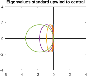
Figure 1: Distribution of eigenvalues for space discretization between standard upwind and central.

In Figure 1, we display the eigenvalues of the discretized linear advection equation using these schemes. While for standard upwind all eigenvalues are on a circle and for central differences on a segment of the imaginary axis, for the other schemes in between, they are located on ellipses. As a consequence, the method we choose for the time integration has to be stable on the convex hull of these ellipses and degenerate ellipses. Apparently, the explicit Euler scheme cannot guarantee stability. Now in Figure 2 we have depicted the boundaries of the stability regions for some standard Runge-Kutta schemes and the root locus curves for Adams-Bashforth methods with up to five old values involved. In both plots, the light blue circle marks the stability region of the explicit Euler method which obviously belongs to both classes. While in both cases the second order method already promises better stability, the stability regions do not yet cover the convex hull of the expected eigenvalues, except for some viscous flows [14]. A closer look reveals that among the Runge-Kutta schemes only RK3 and RK4 yield the desired results. Similarly also in the context of Adams methods, we have to resort to order three or higher.

 

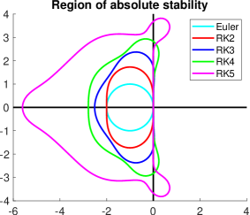
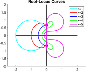
Figure 2: Stability regions for standard schemes. For Adams type schemes, the root locus curves are shown.

A consequence of the sizes of the stability regions is that for Runge-Kutta schemes we can keep the CFL-number from explicit Euler, even increase it somewhat for RK3 and RK4, but for Adams-Bashforth methods, we have to reduce the CFL-number with increasing order. Since for the latter only one flux evaluation is needed per time step, the computational effort is nearly identical for RK and AB methods of the same order, at least for the examples we use in this study. Thus the main remaining question is: How do these schemes perform when applied to the (nonlinear) Euler equations discretized with the Fleischmann solver or our blended schemes? The answer will give us directions for further research and where to look for the ultimate time integration method.

4 Numerical tests

Since, as we have seen in the previous section, third order is sufficient for our purposes, we restrict our comparisons to Euler, RK2, RK3, and AB2, AB3 (short for Adams-Bashforth of the respective order). For some tests, we also include the MUSCL-Hancock method, which obviously is only reasonable in connection with second order in space. Since for orders two and three (and also four) there are several two stage and three stage (and four stage) RK-methods respectively with the same linear stability, we resort to the most traditional ones, namely those connected to the name of Karl Heun:

$$\begin{array}[]{c|cc}0&&\\ 1&1&\\ \hline\cr\\[-6.00006pt] &1/2&1/2\end{array}\qquad\qquad\begin{array}[]{c|ccc}0&&&\\ 1/3&1/3&&\\ 2/3&0&2/3&\\ \hline\cr\\[-6.00006pt] &1/4&0&3/4\end{array}$$

We rechecked with several of the tests and a few other choices for 3rd order three stage Runge-Kutta but could not find a difference. Thus, we will stay with only these two methods.

If not stated otherwise, i. e. for the flow around the infinite cylinder, in the plots we always show the results for the density.

4.1 Uniform low-Mach flow

As our first example, we consider a grid aligned perturbed low-Mach flow. The basic flow is a uniform flow in $x$-direction but superimposed with artificial randomized numerical noise. The Mach number is $M=1/20$. The unperturbed initial values for density and flow velocity (in $x$-direction) are $\rho=1,\ u=1$. The amplitude of the artificial noise on the primitive variables is $10^{-6}$. The final computation time is $t=5$. In the direction of the flow, we employ first order extrapolation at the boundaries, in the transverse direction periodic boundary conditions. Here, we only consider the original Fleischmann solver.

Since this test is a simple 2d-extension of a one-dimensional problem, the results are presented in scatter-type plots: we slice the grid in $x$-direction along the cell faces and plot the density for all slices at once.

Figure 3: Perturbed uniform low-Mach flow with 2nd order time integration: MUSCL Hancock, 2nd order two stage RK (Heun), two step Adams-Bashforth.

In Figure 3 results with 2nd order time integration are shown. It is obvious that AB2 performs superior to MUSCL and RK2. For the latter two, the perturbations increase and, in connection with the extrapolation boundaries, even lead to a significant error in the density. From linear stability theory, perturbations are expected to increase with the 2nd order Adams-Bashforth scheme too. But here in this case the error is much smaller than for the other two methods.

Figure 4: Perturbed uniform low-Mach flow with 3rd order time integration (MUSCL for comparison): MUSCL Hancock, 3rd order three stage RK (Heun), three step Adams-Bashforth.

Looking at Figure 4, RK3 shows no significant improvement compared to RK2. On the other hand, the results with AB3 are perfect as the magnitude of the perturbations does not increase. This confirms that as we suspected above the starting explicit Euler step in each time step of an explicit Runge-Kutta method ruins the stability of the scheme.

4.2 Flow around infinite cylinder

For our second example, we consider the flow around an infinite cylinder, where we expect the solution for low Mach numbers to resemble a potential flow with the pressure forming a quadrupole. If the numerical viscosity on the shear and entropy waves is too high, this might progressively degenerate, eventually leading to a dipole structure [35]. Another issue is that on quadrilateral cells the standard Roe solver is not able to capture the physical solution at all [5]. The reason is that according to an asymptotic analysis for low Mach numbers, the leading order velocity shows incompressibility at cell faces which means that the velocity component perpendicular to the cell face cannot jump over that face. This should be overcome with the Fleischmann solver and, hopefully, also with the blended solvers. Again, the issue might be the stability of the scheme with an unsuited time integration method.

For the tests, we employ the initial setting $\rho=1,p=1$ with different Mach numbers. The computational domain is an annulus with inner radius $r=1$ and outer radius $R=5$ discretized with 160 cells in circumferential and 100 cells in radial direction. At the cylinder we assume wall conditions, at the outer boundary Dirichlet conditions set to the initial state. With these settings, the solution eventually becomes stationary. In the following, the plots show the pressure field for the stationary discrete flow. All computations are done with first order in space.

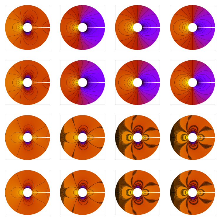
Figure 5: Subsonic flow around infinite cylinder with 3rd order Adams scheme for Mach numbers $10^{-1},\,10^{-2},\,10^{-3},$ and $10^{-4}$ (left to right) with original Roe and 3rd order AB (first row) and RK (second row) as well as the low-Mach solver suggested by Fleischmann et al. also with 3rd order AB (third row) and 3rd order RK (last row).

We start with the 3rd order time integration methods. Figure 5 shows results with the original Roe solver and the low-Mach solver by Fleischmann et al. While the results with the original Roe solver are unphysical as expected for very low Mach numbers, the results with the low-Mach solver are reasonable. Only slight fluctuations can be seen that would be invisible if they were not highlighted by the contour lines. Interestingly, for this example both time integration methods behave similar. This might explain why this issue, which is introduced by the unstable first stage value of explicit Runge-Kutta schemes, was not discovered earlier.

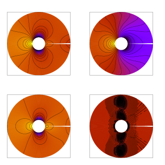
Figure 6: Subsonic flow around infinite cylinder with 2nd order Runge-Kutta scheme for numbers $10^{-1}$ (left) and $10^{-2}$ (right) with original Roe solver (top row) and Fleischmann type solvers (bottom row).

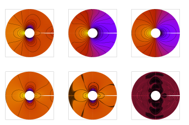
Figure 7: Subsonic flow around infinite cylinder with 2nd order Adams scheme for Mach numbers $10^{-1},\,10^{-2},$ and $10^{-3}$ (left to right) with original Roe (top row) and Fleischmann type solvers (bottom row).

The results with the second order methods are shown in Figures 6 and 7 for Runge-Kutta and Adams-Bashforth respectively. Due to the unstable first stage value, the results for the Runge-Kutta method are inferior to those obtained with the linear multistep method. But, as expected from the stability region, they are also inferior to the results with 3rd order Adams-Bashforth. Already for $M=10^{-3}$ the solution is completely worthless due to heavy oscillations.

4.3 Supersonic blunt body flow

Since we are interested in all-Mach solvers, we also have to include supersonic problems. As a first example we consider a $M=20$ blunt-body flow. As in our previous work [28], we choose an infinite cylinder as test situation, more precisely, a cylinder with radius $r=1$. As computational domain we employ a third of the annulus with inner radius $r=1$ and outer radius $R=2$. Since the interesting part of the flow is the inflow region, we restrict the domain in angular direction to $[{2\pi/3},{4\pi/3}]$. The domain is discretized with 150 cells in the radial direction and 800 cells in the angular direction. The initial flow is set to the inflow state everywhere. At the cylinder, we employ wall boundary conditions, at the other boundaries first order extrapolation.

Figure 8: Mach 20 blunt body flow at time $t=0.5$ with Fleischmann solver and different time integrations: Explicit Euler, Runge-Kutta 2nd and 3rd order, Adams-Bashforth 2nd and third order.

Figure 9: Mach 20 blunt body flow at time $t=2$ with 3rd order Adams-Bashforth and different Riemann solvers: Roe, blended schemes with arithmetic and geometric mean, Fleischmann solver.

The original purpose of Fleischmann et al. [10] was to prevent the carbuncle phenomenon by reducing perturbations in the transverse direction, where the directional Mach number is small. In our case, instabilities of the scheme may also lead to perturbations. Thus, we first compare the different time integration methods in connection with the original Fleischmann solver at an early time. The results are displayed in Figure 8. Obviously, the explicit Euler method and the explicit Runge-Kutta methods, which include an explicit Euler step for the computation of the first stage value, cannot prevent the carbuncle. The results for these schemes are nearly identical. Only with the linear multistep methods, the situation improves. But even with the 3rd order Adams-Bashforth method a carbuncle will form.

In Figure 9, we show the results for a later time with AB3 and different Riemann solvers: original Roe, the blended solvers, and the original Fleischmann solver. Obviously, as was expected from [28], only the blended solvers actually prevent the carbuncle. This means that even with AB3 perturbations are still created in the transverse direction which trigger the instability of the discrete shock profile.

4.4 Richtmyer-Meshkov instability

Figure 10: Initial setting for RMI: In strip $x\in[2,6]$ higher pressure and density, namely $p=4.9,$ and $\rho=4.22$. Otherwise $p=1$, density left and right of sinusoidal boundary $\rho=1$ and $\rho=0.25$.

The so called Richtmyer-Meshkov instability [34] results in a flow field that is comprised of different regimes, clearly compressible regions and nearly incompressible parts. Initially, the flow is at rest. Pressure and density are as sketched out in Figure 10. This causes a shock that runs over the sinusoidal phase boundary and, thus, drives the dynamics of the flow field that eventually leads to a mixing of both the lighter and the heavier fluids. In Figure 11, we show numerical results for the pressure with low-Mach solver as suggested by Fleischmann (left column) and the blended Mach-number consistent solver with the geometrical mean as an all-Mach solver (right column) with both third order 3-stage Runge-Kutta (upper row) and 3rd order Adams-Bashforth (lower row). All computations are with second order in space and a resolution of 600 times 396 cells. The differences between the two Riemann solvers are small. The differences between the time integration methods are, however, much more prominent. Expecially in the low density part with an extremely low Mach number, the results with Runge-Kutta show significant instabilities, as expected from the instability of the first stage value and the results from Section 4.1.

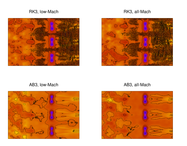
Figure 11: Richtmyer-Meshkov instability, pressure at time $t=85$

4.5 Test examples that leave open questions: Elling and Kelvin-Helmholtz

While the previous results clearly favor Adams methods, there are some examples where no difference exists between Runge-Kutta and Adams-Bashforth like the Elling test, which is a test for a solvers ability to reproduce physical carbuncles [7]. As is indicated in Figure 12, while the original Fleischmann solver performs nicely with MUSCL-Hancock, neither the Runge-Kutta methods nor the Adams-Bashforth methods provide enough stabilization to avoid failure of the computation due to negative internal energy. Even the blended solvers fail.

Figure 12: Elling test with Fleischmann solver and different time integration methods. Except MUSL-Hancock, all fail.

On the other hand, the computation of a Kelvin-Helmholtz instability (Figure 13) yields results for Runge-Kutta and Adams-Bashforth that are correct and nearly indistinguishable while MUSCL-Hancock suffers from the expected instability due to the low viscosity of the Fleischmann solver.

Figure 13: Density for Kelvin-Helmholtz instability with Fleischmann solver and different time integration methods at time $t=4$, contour plot

5 Conclusions and possible directions for further research

We tested some classical explicit time integration methods with the simple low Mach number Riemann solver by Fleischmann et al. as well as with its blended versions. It became apparent that explicit Runge-Kutta methods are not the best choice: The fact that the first stage value is computed with explicit Euler spoils the stability of the resulting scheme. As an alternative we tested some simple Adams-Bashforth methods which behaved considerably better. For many of the more elaborate low-Mach and all-Mach solvers cited in the introduction, they might be sufficient, especially with higher order in space. With very high orders even Runge-Kutta methods may do the job. But for the general case we have to look for further improvement. Some possibilities would be PECE-type methods or general linear methods [25]. For the latter, the stability of stage values has to be taken into account since unstable stage values still could ruin the stability of the scheme.

References

- [1] Francis Bashforth, An attempt to test the theory of capillary action, by J. C. Adams., Cambridge. University press. (1884)., 1884.
- [2] J. C. Butcher, Numerical methods for ordinary differential equations., 2nd revised ed. ed., Hoboken, NJ: John Wiley & Sons, 2008.
- [3] Shu-Sheng Chen, Jin-Ping Li, Zheng Li, Wu Yuan, and Zheng hong Gao, Anti-dissipation pressure correction under low Mach numbers for Godunov-type schemes, Journal of Computational Physics 456 (2022), 111027.
- [4] Shusheng Chen, Boxi Lin, Yansu Li, and Chao Yan, HLLC+: Low-Mach shock-stable HLLC-type riemann solver for all-speed flows, SIAM Journal on Scientific Computing 42 (2020), no. 4, B921–B950.
- [5] Stéphane Dellacherie, Pascal Omnes, and Felix Rieper, The influence of cell geometry on the Godunov scheme applied to the linear wave equation, Journal of Computational Physics 229 (2010), no. 14, 5315–5338.
- [6] Bernd Einfeldt, On Godunov-type methods for gas dynamics., SIAM J. Numer. Anal. 25 (1988), no. 2, 294–318.
- [7] Volker Elling, The carbuncle phenomenon is incurable, Acta Mathematica Scientia 29 (2009), no. 6, 1647–1656.
- [8] L. Ferracina and M. N. Spijker, Stepsize restrictions for the total-variation-diminishing property in general Runge-Kutta methods, SIAM J. Numer. Anal. 42 (2004), no. 3, 1073–1093.
- [9] Nico Fleischmann, Stefan Adami, and Nikolaus A. Adams, A shock-stable modification of the HLLC Riemann solver with reduced numerical dissipation, Journal of Computational Physics 423 (2020), 109762.
- [10] Nico Fleischmann, Stefan Adami, Xiangyu Y. Hu, and Nikolaus A. Adams, A low dissipation method to cure the grid-aligned shock instability, Journal of Computational Physics 401 (2020), 109004.
- [11] Sigal Gottlieb, David Ketcheson, and Chi-Wang Shu, Strong stability preserving Runge-Kutta and multistep time discretizations., Hackensack, NJ: World Scientific, 2011.
- [12] Sigal Gottlieb and Chi-Wang Shu, Total variation diminishing Runge-Kutta schemes, Math. Comput. 67 (1998), no. 221, 73–85.
- [13] Sigal Gottlieb, Chi-Wang Shu, and Eitan Tadmor, Strong stability-preserving high-order time discretization methods, SIAM review 43 (2001), no. 1, 89–112.
- [14] Joseph F Grcar, An explicit Runge-Kutta iteration for diffusion in the low Mach number combustion code, (2007).
- [15] Hervé Guillard and Angelo Murrone, On the behavior of upwind schemes in the low Mach number limit: II. Godunov type schemes, Computers & fluids 33 (2004), 655–675.
- [16] Hervé Guillard and Cécile Viozat, On the behaviour of upwind schemes in the low Mach number limit, Computers & fluids 28 (1999), no. 1, 63–86.
- [17] Ernst Hairer, Christian Lubich, and Gerhard Wanner, Geometric numerical integration. Structure-preserving algorithms for ordinary differential equations, 2nd ed. ed., Springer Ser. Comput. Math., vol. 31, Berlin: Springer, 2006.
- [18] Ernst Hairer, Syvert P. Nørsett, and Gerhard Wanner, Solving ordinary differential equations. I: Nonstiff problems., 2. rev. ed. ed., Springer Ser. Comput. Math., vol. 8, Berlin: Springer-Verlag, 1993.
- [19] Ernst Hairer and Gerhard Wanner, Solving ordinary differential equations. II: Stiff and differential-algebraic problems., 2nd rev. ed. ed., Springer Ser. Comput. Math., vol. 14, Berlin: Springer, 1996.
- [20] K. Heun, Neue Methode zur approximativen Integration der Differentialgleichungen einer unabhängigen Variable., Schlömilch Z. 45 (1900), 23–38.
- [21] Inmaculada Higueras, Representations of Runge-Kutta methods and strong stability preserving methods, SIAM J. Numer. Anal. 43 (2005), no. 3, 924–948.
- [22] Jiří Holman and Jiří Fürst, Rotated-hybrid Riemann solver for all-speed flows, Journal of Computational and Applied Mathematics 427 (2023), 115129.
- [23] Willem Hundsdorfer and Steven J. Ruuth, On monotonicity and boundedness properties of linear multistep methods, Math. Comput. 75 (2006), no. 254, 655–672.
- [24] Willem Hundsdorfer, Steven J. Ruuth, and Raymond J. Spiteri, Monotonicity-preserving linear multistep methods, SIAM J. Numer. Anal. 41 (2003), no. 2, 605–623.
- [25] Zdzisław Jackiewicz, General linear methods for ordinary differential equations, Hoboken, NJ: John Wiley & Sons, 2009.
- [26] A. JAMESON, WOLFGANG SCHMIDT, and ELI TURKEL, Numerical solution of the Euler equations by finite volume methods using runge kutta time stepping schemes.
- [27] Friedemann Kemm, Heuristical and numerical considerations for the carbuncle phenomenon, Appl. Math. Comput. 320 (2018), no. Supplement C, 596–613.
- [28] , Numerical investigation of Mach number consistent Roe solvers for the Euler equations of gas dynamics, Journal of Computational Physics 477 (2023), 111947.
- [29] Xue-Song Li and Chun-Wei Gu, Mechanism of Roe-type schemes for all-speed flows and its application, Computers & Fluids 86 (2013), 56–70.
- [30] Xue-Song Li, Chun-Wei Gu, and Jian-Zhong Xu, Development of Roe-type scheme for all-speed flows based on preconditioning method, Computers & Fluids 38 (2009), no. 4, 810–817.
- [31] K. Oßwald, A. Siegmund, P. Birken, V. Hannemann, and A. Meister, L²Roe: a low dissipation version of Roe’s approximate Riemann solver for low Mach numbers, International Journal for Numerical Methods in Fluids 81 (2016), no. 2, 71–86.
- [32] O. Peles and E. Turkel, Adaptive time steps for compressible flows based on dual-time stepping and a rk/implicit smoother, Journal of Scientific Computing 81 (2019), no. 3, 1409–1428.
- [33] Oren Peles and Eli Turkel, Acceleration methods for multi-physics compressible flow, Journal of Computational Physics 358 (2018), 201–234.
- [34] Robert D. Richtmyer, Taylor instability in shock acceleration of compressible fluids, Communications on Pure and Applied Mathematics 13 (1960), no. 2, 297–319.
- [35] Felix Rieper, On the dissipation mechanism of upwind-schemes in the low Mach number regime: A comparison between Roe and HLL, Journal of Computational Physics 229 (2010), no. 2, 221–232.
- [36] , A low-Mach number fix for Roe’s approximate Riemann solver, Journal of Computational Physics 230 (2011), no. 13, 5263–5287.
- [37] Philip L. Roe, Approximate Riemann solvers, parameter vectors, and difference schemes, J. Comput. Phys. 43 (1981), no. 2, 357–372.
- [38] Cord-Christian Rossow, Efficient computation of compressible and incompressible flows, Journal of Computational Physics 220 (2007), no. 2, 879–899.
- [39] Steven J. Ruuth and Willem Hundsdorfer, High-order linear multistep methods with general monotonicity and boundedness properties, J. Comput. Phys. 209 (2005), no. 1, 226–248.
- [40] Hang Yu, Hua Li, Jianqi Lai, and Ye Zhang, A simple modification of HLLEM approximate Riemann solver applied to the compressible Euler system at Low mach number, IOP Conference Series: Materials Science and Engineering 751 (2020), no. 1, 012002.