Phase diagram of the SU($N$) antiferromagnet of spin $S$ on a square lattice

Abstract

We investigate the ground state phase diagram of an $\text{SU}(N)$-symmetric antiferromagnetic spin model on a square lattice where each site hosts an irreducible representation of $\text{SU}(N)$ described by a square Young tableau of $N/2$ rows and $2S$ columns. We show that negative sign free fermion Monte Carlo simulations can be carried out for this class of quantum magnets at any $S$ and even values of $N$. In the large-$N$ limit, the saddle point approximation favors a four-fold degenerate valence bond solid phase. In the large $S$-limit, the semi-classical approximation points to Néel state. On a line set by $N=8S+2$ in the $S$ versus $N$ phase diagram, we observe a variety of phases proximate to the Néel state. At $S=1/2$ and $3/2$ we observe the aforementioned four fold degenerate valence bond solid state. At $S=1$ a two fold degenerate spin nematic state in which the C₄ lattice symmetry is broken down to C₂ emerges. Finally at $S=2$ we observe a unique ground state that pertains to a two-dimensional version of the Affleck-Kennedy-Lieb-Tasaki state. For our specific realization, this symmetry protected topological state is characterized by an SU(18), $S=1/2$ boundary state, that has a dimerized ground state. These phases that are proximate to the Néel state are consistent with the notion of monopole condensation of the antiferromagnetic order parameter. In particular one expects spin disordered states with degeneracy set by $\text{mod}(4,2S)$.

I Introduction

Spin systems are ubiquitous in nature and form one of the most fundamental concept in condensed matter and statistical physics. Their complex collective behavior has spurred numerous experimental and theoretical studies, aimed at understanding their nature and properties. At the same time, modeling of spin systems represents a primary theoretical laboratory to investigate fundamental physics. Starting with the classical Ising model [1], spin systems have played a crucial role in our understanding of phase transitions [2], phases of matter, frustration and disorder [3], emergent gauge theories [4, 5] and exotic critical behavior [6]. The impact of spin models extends beyond the realm of condensed matter physics, and has found application in other areas, such as information processing [7] and quantum computing [8], where the fundamental unit of information, a qubit, is a single spin-$1/2$ system.

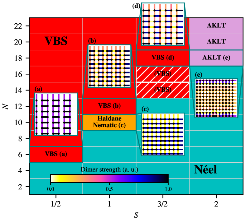
Figure 1: Ground-state phase diagram of the $\text{SU}(N)$-antiferromagnet model (1) on the square lattice, as obtained from QMC simulations. $S$ identifies the chosen representation of the $\mathfrak{su}(N)$ algebra of $\text{SU}(N)$, illustrated by the Young tableau in Fig. 2. Striped regions indicate the part of the phase diagram where current QMC data do not allow an unambiguous identification of the phase; in such cases we indicate between parenthesis the most likely identified order. The insets show QMC data in the highlighted dimerized phases, obtained through a pinning-field approach (see Sec. IV.1).

In condensed matter, spin systems are realized in Mott insulators, which arise when charge fluctuations in a given unit cell are suppressed. For instance, in undoped cuprates the copper atom is in a Cu²⁺ state and corresponds to a net spin $S=1/2$ degree of freedom. Super-exchange leads to an $S=1/2$, SU(2) Heisenberg spin model that has been studied numerically [9, 10] and experimentally [11] at length. Higher spin SU(2) systems arise when $2S$ electrons are localized on a single orbital and a strong Hund’s rule favors a maximal spin state with a totally symmetric wave function. For example, in the Haldane chain realized by the CsNiCl₃ compound Ni²⁺ ions carry spin 1 [12]. $\text{SU}(N)$-invariant models, for $N>2$, naturally arise as special cases of the Kugel-Khomski model [13, 14], where spin and orbital degrees of freedom turn out to play a very symmetric role. In particular, the observed spin-orbital liquid behavior in Ba₃CuSb₂O₉ [15] has been interpreted in terms of an SU(4) quantum antiferromagnet in the defining representation [16]. Beyond the solid state physics, $\text{SU}(N)$ spin models can be realized in the realm of cold atomic gases [17, 18].

Figure 2: Young tableau corresponding to the irreducible representation of $\mathfrak{su}(N)$ considered here; $N$ is even and $S$ is semi-integer.

Topology plays a decisive role in the understanding of SU(2) invariant spin systems. In fact, using a spin coherent-state path integral approach to antiferromagnetic (AFM) Heisenberg chains, one identifies a Berry phase. It corresponds to the skyrmion count of the three-components normalized order parameter in 1+1 dimensions and at angle $\theta=2\pi S$ [19]. This provides a topological understanding of the observed differences between half-integer and integer spin chains. In two spatial dimensions, topology enters through singular skyrmion number changing events in space time: monopoles [20]. For a square lattice with $C_{4}$ symmetry, only quadrupole (double) monopole events are allowed for half-integer (odd) spin by symmetry. There is no constraint on the monopole number for even values of the spin. For the plain vanilla SU(2) Heisenberg model at arbitrary spin $S$, the spin-wave approximation captures well the ground state and topological excitations lie high in the spectrum. In this context, the theory of deconfined quantum criticality essentially poses the question of the nature of the quantum phase transition that emanates when one decreases the energy of monopoles and ultimately condenses them [6, 6]. For half-integer spin systems, where only quadrupole monopole insertions are allowed, one can conjecture that the Hilbert space splits into four orthogonal subspaces characterized by the number of monopoles modulo four. This provides an understanding of how the fourfold degenerate valence bond solid (VBS) state emerges for condensing topological excitations of the quantum antiferromagnet [21]. Similarly, for spin-1 (spin-2) systems, condensing monopoles should generate a twofold (zerofold) degenerate disordered state.

A crucial question is how to control the monopole energy. The seminal work of Read and Sachdev [22, 23, 24] shows that the discussion above can be carried over to $\text{SU}(N)$ spin systems, $N\geq 2$. Furthermore, enhancing $N$ has the potential of lowering the monopole energy. In this paper, we show that it is possible to formulate negative sign-free auxiliary field (AF) quantum Monte Carlo (QMC) simulations [25, 26, 27, 28, 29] of the $\text{SU}(N)$ AFM spin-$S$ Heisenberg model, for representations given by a Young tableau with $N/2$ rows and $2S$ columns. This generalizes the work of Ref. [30] to generic values of $S$. Specifically, we consider the model:

$$\hat{H}=J\sum_{\langle i,j\rangle,a}\hat{S}^{(a)}_{i}\hat{S}^{(a)}_{j},$$ (1)

where the sum extends over the pair of nearest-neighbor sites $\langle i,j\rangle$, and $a$ runs over $N^{2}-1$ generators of the said representation of the $\mathfrak{su}(N)$ algebra of $\text{SU}(N)$. The main result of this paper is the rich phase diagram illustrated in Fig. 1. Remarkably, and for each considered value of $S=1/2,1,3/2,2$ just above the threshold value of $N$ above which Néel order disappears, we observe four-, two- and zerofold degenerate disordered states at half-integer, odd and even values of $S$.

This paper is organized as follows. In Sec. II we discuss how we construct the Hamiltonian (1), with the spin operators in the desired representation of Fig. 2. In Sec. III we illustrate its actual implementation within a fermionic representation, which can be sampled by means of QMC simulations in the AF approach. In Sec. IV we present and discuss our QMC results for the phase diagram of the model. In Sec. V we summarize our findings. In Appendix A we discuss a formula giving the eigenvalue of the quadratic Casimir operator of a representation in terms of its Young tableau. In Appendix B we prove an upper bound on the eigenvalue of the Casimir operator of the irreducible representations emerging from a tensor product of representations discussed in Sec. II. In Appendix C we discuss the systematic error in the QMC formulation, arising from the Trotter discretization. In Appendix D we prove a lower and upper bound for a bond observable used to diagnose the phases.

II General formulation of the Hamiltonian

In the Hamiltonian (1), the operators $S^{(a)}_{i}$ form an irreducible representation of the $\mathfrak{su}(N)$ algebra. This is uniquely specified by its maximum Dynkin weight $\Lambda_{\alpha}$ or, alternatively, by a Young tableau, from which the components $\Lambda_{\alpha_{k}}$ can be read off as [31]

$$\Lambda_{\alpha_{k}}=l_{k}-l_{k+1},\qquad k=1,\ldots,N-1,$$ (2)

where $l_{k}$ is the length of the $k$-th row of the Young tableau, and one can assume $l_{N}=0$ for representations of $\mathfrak{su}(N)$.

Here we consider, on each lattice site, the representation corresponding to a Young tableau illustrated in Fig. 2, whose corresponding maximum Dynkin weight is

$$\Lambda_{\alpha_{k}}=2S\delta_{k,N/2}.$$ (3)

The dimension of an irreducible representation can be computed with the hook-length formula, or with Weyl’s formula [31]:

$$\text{dim}=\prod_{i<j}^{N}\frac{l_{i}-l_{j}+j-i}{j-i}.$$ (4)

For the present case, we have

$$\text{dim}=\prod_{j=0}^{N/2-1}\frac{\left(2S+\frac{N}{2}+j\right)!j!}{\left(2S+j\right)!\left(\frac{N}{2}+j\right)!}.$$ (5)

To realize this representation, we first introduce on each lattice site $2S$ independent irreducible representations. Their tensor product decomposes into different irreducible representations, including, in particular, the one of Fig. 2. In a second step, we project the Hilbert space onto that of the desired representation by maximizing the quadratic Casimir operator.

Let $\{T_{a}\}$, $a=1,\ldots,N^{2}-1$ be a basis of the $\mathfrak{su}(N)$ algebra. We start by introducing on each lattice site $i$ the antisymmetric self-adjoint representation $T_{a}\rightarrow\Gamma(T_{a})=\hat{T}_{a,i}$. Its maximum weight in the Dynkin representation is

$$\Lambda_{\alpha_{k}}=\delta_{k,N/2},$$ (6)

which matches Eq. (3) for $S=1/2$. Equivalently, in agreement with Eq. (2), this representation corresponds to a Young tableau with one column and $N/2$ boxes.

Figure 3: Decomposition of the tensor product of $2S$ antisymmetric self-adjoint representations, whose maximum Dynkin weight is given in Eq. (6), into irreducible ones.

Next, we consider, for each lattice site $i$, $2S$ independent representations $\hat{T}_{a,i,\alpha}$, $\alpha=1\ldots 2S$. We refer to $\alpha$ as the flavor index. The composite generators, i.e., the generators for the tensor product of the $2S$ representations, define the spin operators appearing in Eq. (1) and are given by

$$\hat{S}_{i}^{(a)}=\sum_{\alpha=1}^{2S}\hat{T}_{a,i,\alpha},$$ (7)

Using Eq. (7), the interaction term in Eq. (1) is written as

$$\begin{split}\hat{H}_{J}&=J\sum_{\langle i\ j\rangle}\sum_{a=1}^{N^{2}-1}\hat{S}^{(a)}_{i}\hat{S}^{(a)}_{j}\\ &=J\sum_{\langle i\ j\rangle}\sum_{a=1}^{N^{2}-1}\sum_{\alpha,\beta=1}^{2S}\hat{T}_{a,i,\alpha}\hat{T}_{a,j,\beta}.\end{split}$$ (8)

The operators $\hat{S}_{i}^{(a)}$ in Eq. (7) form a reducible representation of $\mathfrak{su}(N)$, which decomposes into several irreducible representations, illustrated in Fig. 3. As proven in App. B, among the resulting representations, the one of Fig. 2 exhibits the maximum eigenvalue of the quadratic Casimir operator. To explicitly compute it, we choose a basis $\{T_{a}\}$ of $\mathfrak{su}(N)$ such that

$$\text{Tr}\{T_{a}T_{b}\}=\frac{1}{2}\delta_{ab}.$$ (9)

With this choice, the structure constants of the algebra are completely antisymmetric and the chosen basis is, up to a trivial normalization, self-dual with respect to the bilinear form (9). Thus, given an irreducible representation $\Gamma:\mathfrak{su}(N)\rightarrow GL(d,\mathbb{C})$, we define the quadratic Casimir operator as

$$\hat{C}_{2}=\sum_{a}\Gamma(T_{a})\Gamma(T_{a})\equiv C\mathbb{1}_{d},$$ (10)

where we have used the fact that $C_{2}\propto\mathbb{1}_{d}$ (Schur’s Lemma) to introduce the eigenvalue of the Casimir operator $C$ . Using Eq. (7) in Eq. (10), the quadratic Casimir operator on the lattice site $i$ is

$$\hat{C}_{2,\Gamma_{i}}=\sum_{a=1}^{N^{2}-1}\sum_{\alpha,\beta=1}^{2S}\hat{T}_{a,i,\alpha}\hat{T}_{a,i,\beta}$$ (11)

In order to project the Hilbert space to the subspace of the desired representation, we introduce on each site a term in the Hamiltonian which favors the states with the highest Casimir value

$$\begin{split}\hat{H}_{\text{Casimir}}&=-J_{H}\sum_{i}\hat{C}_{2,\Gamma_{i}}\\ &=-J_{H}\sum_{i}\sum_{a=1}^{N^{2}-1}\sum_{\alpha,\beta=1}^{2S}\hat{T}_{a,i,\alpha}\hat{T}_{a,i,\beta},\end{split}$$ (12)

with $J_{H}>0$. The term of Eq. (12) effectively introduces a ferromagnetic interaction between different flavors, with coupling strength $J_{H}$.

The Hamiltonian that we will solve numerically, reads:

$$\hat{H}=\hat{H}_{J}+\hat{H}_{\text{Casimir}}.$$ (13)

Importantly, $\left[\hat{H}_{J},\hat{H}_{\text{Casimir}}\right]=0$, such that the projection onto the desired irreducible representation turns out to be very efficient. And since the projection is a local onsite term, we expect it to scale independent from system size.

III QMC formulation

III.1 Fermionic representation

As discussed in Sec. II, the Hamiltonian is constructed using as basic building blocks antisymmetric self-adjoint representations, defined by the maximum weight of Eq. (6) or, equivalently, by a Young tableau with one column and $N/2$ boxes. The corresponding operators $\hat{T}_{a,i,\alpha}$ entering in Eqs. (8) and (12) can be realized by introducing, for every lattice site $i$ and for every flavor index $\alpha$, $N$ nonrelativistic fermions, with creation and annihilation operators $\hat{c}_{i,\alpha,\sigma}^{\dagger}$, $\hat{c}_{i,\alpha,\sigma}^{\phantom{{\dagger}}}$, $\sigma=1\ldots N$, and fixing the total charge (i.e., the number of fermions) to half-filling, i.e., to $N/2$. For every $i$ and $\alpha$, a basis of this Hilbert space is generated by the states

$$\left(\hat{c}_{i,\alpha,1}^{\dagger}\right)^{n_{i,\alpha,1}}\cdots\left(\hat{c}_{i,\alpha,N}^{\dagger}\right)^{n_{i,\alpha,N}}|0\rangle,\qquad n_{i,\alpha,\sigma}=0,1,$$ (14)

with the constraint

$$\sum_{\sigma=1}^{N}n_{i,\alpha,\sigma}=\frac{N}{2},\qquad\forall i,\alpha.$$ (15)

In this space, the (representation of the) $\mathfrak{su}(N)$ generators are

$$\hat{T}_{a,i,\alpha}=\sum_{\sigma,\sigma^{\prime}}\hat{c}_{i,\alpha,\sigma}^{\dagger}(T_{a})_{\sigma\sigma^{\prime}}\hat{c}_{i,\alpha,\sigma^{\prime}}^{\phantom{{\dagger}}}.$$ (16)

It is easy to check that the maximum weight in the Dynkin representation agrees with Eq. (6), thus providing us the needed building block to simulate the Hamiltonian (1).

We study the model by means of finite-temperature AF QMC [28, 25, 26] and projective AF QMC [34, 27, 28]. In this framework, we sample respectively the grand canonical and canonical ensembles at half-filling, and charge fluctuations are generally present. Therefore, we need to additionally impose the constraint of Eq. (15). Notice that, unlike available techniques for canonical QMC simulations [35, 36], where the global charge of the system is fixed, here we need to impose half-filling on each lattice site. To this end, we add a repulsive Hubbard $U$-term on each site $i$ and flavor $\alpha$:

$$\hat{H}_{U}=U\sum_{i}\sum_{\alpha=1}^{2S}\left(\hat{n}_{i,\alpha}-\frac{N}{2}\right)^{2},\quad\hat{n}_{i,\alpha}\equiv\sum_{\sigma=1}^{N}\hat{c}_{i,\alpha,\sigma}^{\dagger}\hat{c}_{i,\alpha,\sigma}^{\phantom{{\dagger}}}.$$ (17)

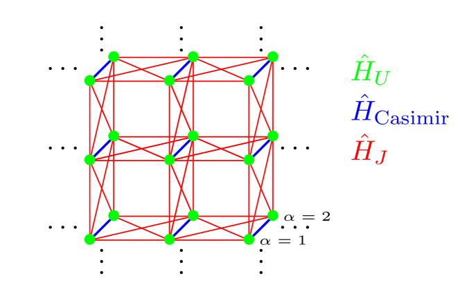
Figure 4: Sketch of the structure of the QMC Hamiltonian for $2S=2$. $\hat{H}_{U}$: Hubbard term for freezing out charge degrees of freedom. $\hat{H}_{\text{Casimir}}$: Term for maximizing the eigenvalue of the Casimir operator. $\hat{H}_{J}$: Antiferromagnetic interaction between elemental spins.

In summary, the Hamiltonian simulated with the AF QMC method is the sum of the interaction term given in Eq. (8), the Casimir term [Eq. (12)], and the Hubbard term [Eq. (17)], with the operators $\{\hat{T}_{a,i,\alpha}\}$ given in Eq. (16). Eqs. (8) and (12) can be further simplified using the following summation identity [37]

$$\sum_{a=1}^{N^{2}-1}(T_{a})_{\sigma\sigma^{\prime}}(T_{a})_{\epsilon\epsilon^{\prime}}=\frac{1}{2}\left(\delta_{\sigma\epsilon^{\prime}}\delta_{\sigma^{\prime}\epsilon}-\frac{1}{N}\delta_{\sigma\sigma^{\prime}}\delta_{\epsilon\epsilon^{\prime}}\right),$$ (18)

which holds for a choice of generators that satisfies Eq. (9). Using Eq. (18) and collecting the terms in Eqs. (8), (12) and (17), the QMC Hamiltonian is

$$\begin{split}\hat{H}_{\text{QMC}}=&\hat{H}_{J}+\hat{H}_{\text{Casimir}}+\hat{H}_{U}\\ =&-\frac{J}{4}\sum_{\langle i,j\rangle,\alpha,\beta}\left\{\hat{D}_{(i,\alpha),(j,\beta)},\hat{D}^{\dagger}_{(i,\alpha),(j,\beta)}\right\}\\ &+\frac{J_{H}}{2}\sum_{i}\sum_{\alpha>\beta}\left\{\hat{D}_{(i,\alpha),(i,\beta)},\hat{D}^{\dagger}_{(i,\alpha),(i,\beta)}\right\}\\ &+U\sum_{i,\alpha}\left(\hat{n}_{i,\alpha}-\frac{N}{2}\right)^{2},\\ \end{split}$$ (19)

where

$$\hat{D}_{(i,\alpha),(j,\beta)}\equiv\sum_{\sigma}\hat{c}_{i,\alpha,\sigma}^{\dagger}\hat{c}_{j,\beta,\sigma}^{\phantom{{\dagger}}},$$ (20)

$\left\{\hat{A},\hat{B}\right\}\equiv\hat{A}\hat{B}+\hat{B}\hat{A}$, and $\hat{n}_{i,\alpha}$ as defined in Eq. (17). The Hamiltonian now takes the form of the Heisenberg model considered in Ref. [30] and the proof for the absence of sign problem is similar. In Fig. 4 we sketch the resulting interactions for the case $S=1$.

Before proceeding, we would like to comment on the computational cost of the AF QMC algorithm [28] for this model. The total number of orbitals is given by $L^{2}2S$ such that matrix operations required to compute, e.g., the single-particle spectral function, scales as $(L^{2}2S)^{3}\beta$, where $\beta$ is the inverse temperature. It turns out, that, in contrast to the generic Hubbard model with $L^{2}2S$ sites, this is not the leading computational cost. The number of Hubbard-Stratonovitch fields per imaginary time slice scales as $L^{2}S^{2}$. Using fast updates, refreshing one field involves $(L^{2}2S)^{2}$ floating point operations, such that the total cost of the updating scales as $L^{6}S^{4}\beta$. Hence large values of $S$ are computationally expensive. In Appendix C, we show that the computational cost does not explicitly scale with $N$. We note that this estimate of the computational cost does not take into account auto-correlation times.

III.2 Test of projections

As discussed above, the Hamiltonian (19) is equivalent to Eq. (1) in the limit $J_{H}\rightarrow\infty$, and $U\rightarrow\infty$, under which the Hilbert space is projected to the representation of Fig. 2. To optimally test the projections, we use the finite-temperature AF QMC method, which evaluates $\langle\hat{O}\rangle=\text{Tr}\left[e^{-\beta\hat{H}}\hat{O}\right]/\text{Tr}\left[e^{-\beta\hat{H}}\right]$, where the trace runs over the grand canonical ensemble.

The interaction term of Eq. (8) and the Casimir term of Eq. (12) manifestly conserve the charge on each lattice site $i$. Hence, in the Gibbs density matrix $\exp(-\beta\hat{H})$, the Hubbard term factorizes out, resulting in an effective exponential suppression of the charge fluctuations,

$$\Braket{\left(\hat{n}_{i,\alpha}-N/2\right)^{2}}\propto e^{-\beta U},$$ (21)

independent from system size. The suppression of charge fluctuations is therefore particularly efficient. This is illustrated in Fig. 5, where we show $\langle\left(\hat{n}_{i,1}-N/2\right)^{2}\rangle$ in a semilogarithmic scale for $N=2$ and $S=1/2$ and as a function of $\beta U$. Besides the case of a Hamiltonian containing the Hubbard interaction [Eq. (17)] only, for which any observable depends only on $\beta U$, we consider the presence of the AFM interaction Eq. (8) for a lattice of linear size $L=4$. In the latter case, there is an additional dependence on the inverse temperature $\beta$, which we illustrate by considering four values. In line with Eq. (21), we observe an exponential suppression of the charge fluctuations as a function of $\beta U$. Interestingly, in the interacting case, $\langle\left(\hat{n}_{i,1}-N/2\right)^{2}\rangle$ decreases with the temperature for any given value of $\beta U$, even for $U=0$. This implies that the AFM coupling itself suppresses the charge fluctuations.

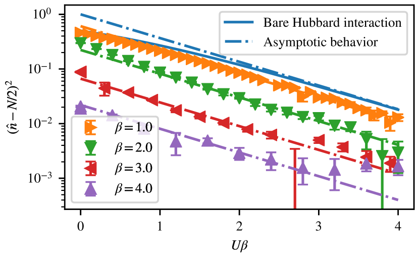
Figure 5: Suppression of the charge fluctuations $\langle\left(\hat{n}_{i,1}-N/2\right)^{2}\rangle$ as a function of $\beta U$, for $N=2$ and $S=1/2$. We consider a Hamiltonian containing the Hubbard term only and the case of a model with an antiferromagnetic interaction [Eq. (8)], with coupling constant $J=1$ on a system size $L=4$, and for different inverse temperatures $\beta$. The charge fluctuations fall off asymptotically as $\exp(-\beta U)$ [Eq. (21)].

In Appendix A, we discuss a formula that gives the value of the Casimir eigenvalue in terms of the Young tableau of the representation [38]. Employing this result, in Appendix B we determine, for the representation of Fig. 2:

$$C(N,S)=\frac{NS(2S+N)}{4}.$$ (22)

Furthermore, in Appendix B, we prove that Eq. (22) is the maximum Casimir eigenvalue among the irreducible representations arising from the tensor product of $2S$ self-adjoint antisymmetric representations given in Eq. (16), and that there is a finite gap $O(1)$ in the eigenvalues of the quadratic Casimir operators between the maximally symmetric representation of Fig. 2 and the other irreducible representations arising from the tensor product. Therefore, the term of Eq. (12) effectively selects a single representation, and the projection is efficient.

To control the projection, we compute the expectation value of the quadratic Casimir operator from the QMC simulations and compare it with the expected result of Eq. (22). An example of such a projection is shown in Figs. 6 and 7. In Fig. 6, we plot the difference between the computed and expected Casimir eigenvalue $C$, as a function of $\beta J_{H}$, for different inverse temperatures and in a semilogarithmic scale. The deviation from the expected result is exponentially suppressed in $\beta J_{H}$, underscoring the effectiveness of the projection. In Fig. 7, we show, as a function of $N$, the sampled value of $C$ along with the expected result, and in the inset we plot their difference, which vanishes within error bars.

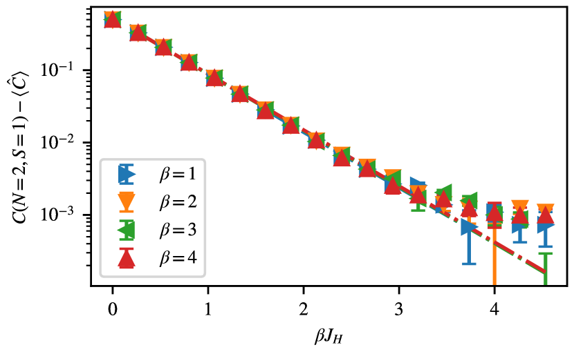
Figure 6: Difference between the Casimir eigenvalue $C(N=2,S=1)$ [Eq. (22)] of the representation $S=1$, $N=2$, and the sampled one $\langle\hat{C}\rangle$, as a function of the effective interaction strength $\beta J_{H}$ [Eq. (12)] with $J=0$, and for four inverse temperatures. Data shown are obtained for a lattice of size $L=4$, with a Hubbard interaction $\beta U=6$ [Eq. (17)], vanishing nearest-neighbor antiferromagnetic interaction $J=0$, and a Trotter discretization $\Delta\tau=0.1$.

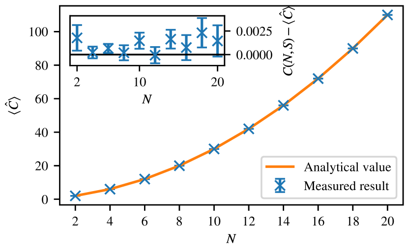
Figure 7: Casimir eigenvalue for representations with $S=1$ and as a function of $N$. We compare the predicted value of Eq. (22) with the sampled Casimir eigenvalue from QMC simulations of a lattice with size $L=4$, with a Hubbard interaction $U=2$ [Eq. (17)], antiferromagnetic coupling $J=1$ [Eq. (1)], projection strength $J_{H}=1$ [Eq. (12)], and a Trotter discretization $\Delta\tau=0.1$. In the inset we plot the difference between the sampled and expected value.

IV Results

IV.1 Order parameters and phases

We have simulated the Hamiltonian Eq. (19) using the ALF package [39, 29], which provides a comprehensive library to program QMC simulations of interacting models of fermions, using the AF algorithm [28, 25, 26]. In particular, we used the projective formulation of the algorithm, which projects a trial wave function $\ket{\Psi_{\rm T}}$ onto the ground state of the system. Observables are evaluated through

$$\braket{\hat{O}} =\frac{\Braket{\Psi_{\rm T}}{e^{-\Theta\hat{H}}\hat{O}e^{-\Theta\hat{H}}}{\Psi_{\rm T}}}{\Braket{\Psi_{\rm T}}{e^{-2\Theta\hat{H}}}{\Psi_{\rm T}}},$$ (23)

with $\Theta$ the projection parameter. The algorithm employs a Hubbard-Stratonovich decomposition of the interaction terms. This results in a free fermionic system, where any observable can be computed via the Wick’s theorem from the Green’s functions. The QMC method consists in a stochastic sampling of the Hubbard-Stratonovich fields. We refer to Ref. [28] for a discussion of the AF QMC method.

As trial wave function $\ket{\Psi_{\rm T}}$, we used the half-filled ground state of

$$\hat{H}_{\rm T}=\sum_{\langle i,j\rangle}\sum_{\alpha=1}^{2S}\left(\hat{D}_{(i,\alpha),(j,\alpha)}+{\rm H.c.}\right).$$ (24)

We scaled the projection parameter $\Theta$ with linear system size $L$, usually comparing the results obtained with $\Theta=L/4$ and $\Theta=L/2$, ensuring that they reflect ground state properties. Furthermore, we chose the parameters for suppression of charge fluctuations and projection onto the maximally symmetric representation around $U=4/\Theta$, $J_{H}=4/\theta$, while always checking that charge fluctuations are sufficiently suppressed and $\braket{\hat{C}}=C(N,S)$ [cf. Eq. (22)].

To detect the realization of different ground states, we have sampled the spin two-point function $S(\boldsymbol{k})$ and the correlations of the dimer operator $D_{ij}(\boldsymbol{k})$ in momentum space, defined as

$$S(\boldsymbol{k})\equiv\frac{1}{(N^{2}-1)N_{r}^{2}} \sum_{\boldsymbol{r},a}e^{i\boldsymbol{k}\boldsymbol{r}}\Braket{\hat{S}^{(a)}_{\boldsymbol{0}}\hat{S}^{(a)}_{\boldsymbol{r}}},$$ (25)

$$\begin{split}D_{ij}(\boldsymbol{k})\equiv\frac{1}{(N^{2}-1)N_{r}^{2}}&\sum_{\boldsymbol{r},a,b}e^{i\boldsymbol{k}\boldsymbol{r}}\cdot\\ \Bigg{[}&\Braket{\left(\hat{S}^{(a)}_{\boldsymbol{0}}\hat{S}^{(a)}_{\boldsymbol{0}+\boldsymbol{e}_{i}}\right)\left(\hat{S}^{(b)}_{\boldsymbol{r}}\hat{S}^{(b)}_{\boldsymbol{r}+\boldsymbol{e}_{j}}\right)}\\ &-\Braket{\hat{S}^{(a)}_{\boldsymbol{0}}\hat{S}^{(a)}_{\boldsymbol{0}+\boldsymbol{e}_{i}}}\Braket{\hat{S}^{(b)}_{\boldsymbol{r}}\hat{S}^{(b)}_{\boldsymbol{r}+\boldsymbol{e}_{j}}}\Bigg{]},\end{split}$$ (26)

where $N_{r}=L^{2}$ is the number of sites in a lattice of linear size $L$ and $\boldsymbol{e}_{i}$ is the elementary lattice unit vector on the $i-$th direction. The normalization in Eqs. (25) and (26) ensure a finite thermodynamic and large-$N$ limit. Using these observables, we can distinguish the Néel state and different dimerized ground states, to be discussed below.

The AFM Néel state exhibits long-range spin-spin correlations at momentum $\boldsymbol{k}=(\pi,\pi)$. Thus, it can be detected by the staggered magnetization $m$

$$m^{2}=S(\boldsymbol{k}=(\pi,\pi)).$$ (27)

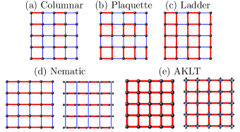
Figure 8: Sketch of possible dimerized ground states. (a)-(c) The VBS states. Each of those states is fourfold degenerate, the corresponding states can be obtained by rotations and translations. (d) A “Haldane nematic” state, an equivalent state is obtained by rotations of $90^{\circ}$. (e) A unique ground state. States (d) and (e) are at best understood within an AKLT construction, in which, very much as done in our calculation, the spin $S$ on each site is constructed by a totally symmetric superposition of $2S$ states that are denoted by bullets around each site on the right-hand side of (d) and (e). These bullets correspond to an irreducible representation of $\mathfrak{su}(N)$ with one column ($S=1/2$) and $N/2$ rows. In the nematic state, each spin-$1/2$ forms a singlet with the nearest neighbor along the axis of the broken symmetry. The AKLT state is relevant for the $S=2$ state, where each spin-$1/2$ on a given site can be combined into a singlet with a nearest-neighbor spin-$1/2$ without breaking a lattice symmetry.

The valence bond state (VBS) breaks the lattice rotation and translation symmetries, realizing a fourfold degenerate pattern of strong and weak dimers. This is realized by different sets of bond configurations, illustrated in Figs. 8(a)-8(c). Beyond the commonly identified columnar order, sketched in Fig. 8(a), there are two additional VBS states [Figs. 8(b) and 8(c)]. Notably, all three patterns break the lattice translation symmetry, but only columnar and ladder order break the four-fold rotation symmetry. VBS order can be detected by a suitable order parameter $\phi$ defined in terms of the dimer correlations

$$\phi^{2}\equiv D_{xx}(\boldsymbol{k})+D_{yy}(\boldsymbol{k}),\qquad\boldsymbol{k}=(\pi,0).$$ (28)

We average $\phi$ over the two equivalent momenta $(\pi,0)$, and $(0,\pi)$ as to obtain an improved estimator.

For integer values of $S$, we investigate the possible realization of the “Haldane nematic” Affleck-Kennedy-Lieb-Tasaki (AKLT) phase [40, 22, 23, 24]. This state is twofold degenerate and breaks the rotational symmetry but, unlike the VBS state, does not break translational symmetry. We illustrate it in Fig. 8(d). For such a phase we have $\phi=0$ and a suitable order parameter can be defined as [41]

$$\psi^{2}\equiv D_{xx}(\boldsymbol{k})+D_{yy}(\boldsymbol{k})-D_{xy}(\boldsymbol{k})-D_{yx}(\boldsymbol{k}),\qquad\boldsymbol{k}=\boldsymbol{0}.$$ (29)

$\psi$ is designed to pick up rotation symmetry breaking in the dimers and therefore does also not vanish for columnar and ladder order. Therefore, $\psi$ distinguishes plaquette with $C_{4}$ symmetry from VBS order with broken $C_{4}$ symmetry.

Finally, a two-dimensional version of the AKLT phase, with singlets on all bonds as sketched in Fig. 8(e), is also possible for $S=2$. This non-degenerate state does not break any symmetry, therefore all previously defined order parameters vanish. In Table 1 we summarize the different orders.

Table 1: List of considered ground states with their ordering momenta in reciprocal space and matrix of order parameters defined in Eqs. (27), (28), (29).

Phase	Ordering momenta	$C_{4}$ Lattice symmetry preserved	$m$	$\phi$	$\psi$
Néel	$(\pi,\pi)$	yes	$\neq 0$	$0$	$0$
Columnar	$(\pi,0)$ or $(0,\pi)$	no	$0$	$\neq 0$	$\neq 0$
Plaquette	$(\pi,0)$ and $(0,\pi)$	yes	$0$	$\neq 0$	$0$
Ladder	$(\pi,0)$ or $(0,\pi)$	no	$0$	$\neq 0$	$\neq 0$
Nematic	$(0,0)$	no	$0$	$0$	$\neq 0$
2d AKLT	$(0,0)$	yes	$0$	$0$	$0$

Given a local order parameter $O$ at momentum $\boldsymbol{p}$, one can define the correlation ratio $R_{O}$ as

$$R_{O}\equiv 1-\frac{C_{O}(\boldsymbol{p}+\delta\boldsymbol{p})}{C_{O}(\boldsymbol{p})},$$ (30)

where $C_{O}(\boldsymbol{p})$ is the two-point function of the order parameter in Fourier space, and $\delta\boldsymbol{p}$ is the minimum nonzero momentum on a finite lattice. On the square lattice, $\delta\boldsymbol{p}=(2\pi/L,0)$ or $\delta\boldsymbol{p}=(0,2\pi/L)$; as usual, one can average over the two minimum displacements to obtain an improved estimator. The correlation ratio is closely related to the second-moment finite-size correlation length $\xi$, which on a square lattice can be defined as [42, 43]

$$\xi=\frac{1}{2\sin(\pi/L)}\sqrt{\frac{C_{O}(\boldsymbol{p})}{C_{O}(\boldsymbol{p}+\delta\boldsymbol{p})}-1}.$$ (31)

In a disordered phase, $\xi$ as defined in Eq. (31) converges to the second-moment correlation length for $L\rightarrow\infty$, such that $\xi/L\rightarrow 0$ and $R_{0}\rightarrow 0$. In an ordered phase, due to the lack of spontaneous symmetry breaking in any finite size, $\xi/L$ diverges for $L\rightarrow\infty$ and, conversely, $R_{0}\rightarrow 1$. In the vicinity of a critical point, $R_{O}$ and $\xi/L$ are renormalization-group invariant quantities. Their crossing can be used to locate the onset of the phase transition, rendering them powerful quantities to diagnose the ground-state order and to study phase transitions.

An ergodic QMC simulation averages over all symmetry-breaking states. As a result, we are not able to observe the ordered state directly, but have to refer to correlation functions that do not average out to zero when averaging over all degenerate ground states. Unfortunately, such an approach does not distinguish between the different VBS states illustrated in Figs. 8(a)-8(c). To obtain additional insights we use the method of a pinning field [44, 45]. In this approach, we explicitly break the symmetry by making one AFM interaction at the origin $J_{\text{pin}}\sum_{a}\hat{S}^{(a)}_{\boldsymbol{0}}\hat{S}^{(a)}_{\boldsymbol{0}+\boldsymbol{e}_{\rm x}}$ stronger than the other interactions $J\sum_{a}\hat{S}^{(a)}_{\boldsymbol{r}}\hat{S}^{(a)}_{\boldsymbol{r}+\boldsymbol{e}_{i}}$. The resulting Hamiltonian reads:

$$\hat{H} =J\sum_{(\boldsymbol{r},i)\neq(\boldsymbol{0},{\rm x})}\sum_{a}\hat{S}^{(a)}_{\boldsymbol{r}}\hat{S}^{(a)}_{\boldsymbol{r}+\boldsymbol{e}_{i}}+J_{\text{pin}}\sum_{a}\hat{S}^{(a)}_{\boldsymbol{0}}\hat{S}^{(a)}_{\boldsymbol{0}+\boldsymbol{e}_{\rm x}},$$ (32)

with $J_{\text{pin}}>J$. Therefore, we explicitly choose one of multiple degenerate ground states by pinning the bond $(\boldsymbol{0},\boldsymbol{0}+\boldsymbol{e}_{\rm x})$ and the bond observable

$$B_{i}(\boldsymbol{r})\equiv\frac{1}{C(N,S)}\Braket{\sum_{a}\hat{S}^{(a)}_{\boldsymbol{r}}\hat{S}^{(a)}_{\boldsymbol{r}+\boldsymbol{e}_{i}}}\qquad i={\rm x,y}$$ (33)

does not vanish as in the unpinned case. We notice that the AFM interactions in the Hamiltonian favors a minimization of $B_{i}(\boldsymbol{r})$. As proven in Appendix D, $B_{i}(\boldsymbol{r})\geq-1$ and approaches $-1$ when the two spins form a singlet.

We have chosen $J_{\text{pin}}$ such that the pinned bond satisfies

$$\Braket{\sum_{a}\hat{S}^{(a)}_{\boldsymbol{0}}\hat{S}^{(a)}_{\boldsymbol{0}+\boldsymbol{e}_{\rm x}}}\\ \approx\frac{1}{2}\left(\frac{1}{2N_{r}}\sum_{(\boldsymbol{r},i),a}\Braket{\hat{S}^{(a)}_{\boldsymbol{r}}\hat{S}^{(a)}_{\boldsymbol{r}+\boldsymbol{e}_{i}}}-C(N,S)\right).$$ (34)

The right-hand side corresponds to the point halfway between the background and the minimal value of $\Braket{\sum_{a}\hat{S}^{(a)}_{\boldsymbol{0}}\hat{S}^{(a)}_{\boldsymbol{0}+\boldsymbol{e}_{\rm x}}}$. This results in $J_{\text{pin}}$ between $1.2J$ and $1.5J$.

At large distances from the pinned bond, one will either be able to explicitly observe the “selected” order through $B_{i}(\boldsymbol{r})$ (if $\phi$ or $\psi$ are nonzero), or the order will vanish.

IV.2 $S=1/2$

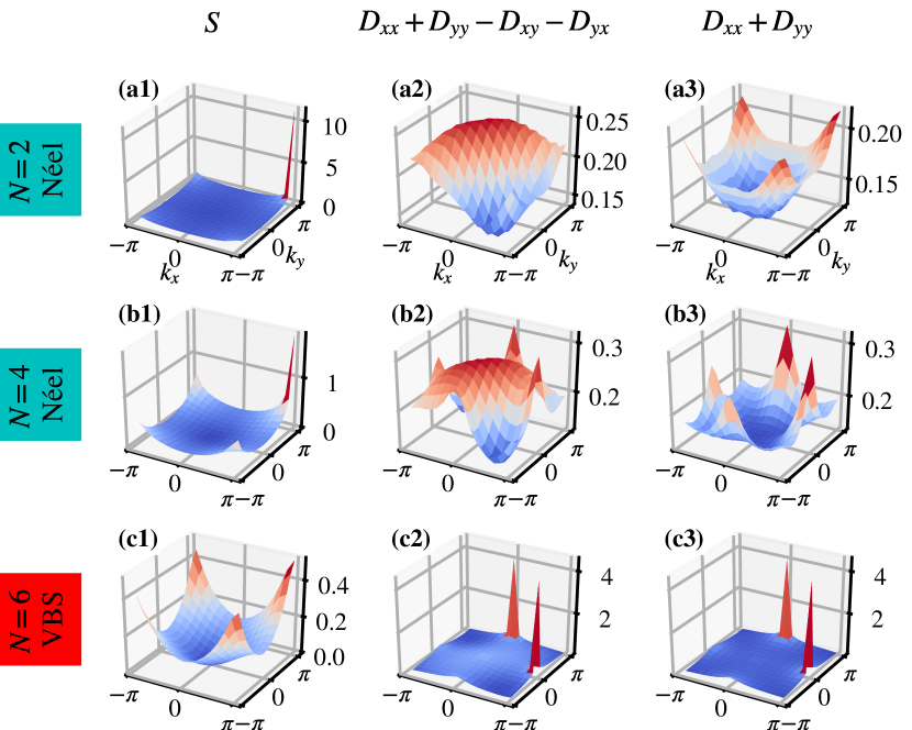
Figure 9: Correlation functions $S(\boldsymbol{k})$ [Eq. (25)] and $D_{ij}(\boldsymbol{k})$ [Eq. (25)] for the representation of Fig. 2 with $S=1/2$ and different values of $N$.

We first study the representations of Fig. 2 with $S=1/2$. In Fig. 9, we show the structure factor $S(\boldsymbol{k})$ [Eq. (25)], and the two combinations of dimer correlations $D_{ij}(\boldsymbol{k})$ appearing in the definitions of the order parameter $\phi$ [Eq. (28)] and $\psi$ [Eq. (29)]. By considering three values of $N$, we analyze the evolution of the order parameters across the transition between the Néel and VBS order. For $N=2$, we realize a standard $S=1/2$ Heisenberg model on the square lattice, which displays a Néel order in the ground state. As expected, $S(\boldsymbol{k})$ shows a strong peak at $(\pi,\pi)$; in comparison, the other order parameters are suppressed. Upon increasing $N$ to $N=4$, we observe the emergence of peaks at $(\pi,0)$ and $(0,\pi)$ for the other order parameters. As shown below using the correlation ratios, though close to the phase transition to the VBS state, the ground state is still Néel ordered. For $N=6$ we observe a strong peak at $(\pi,0)$ and $(0,\pi)$ for the $D_{xx}(\boldsymbol{k})+D_{yy}(\boldsymbol{k})$ order parameters, indicating the realization of the VBS phase.

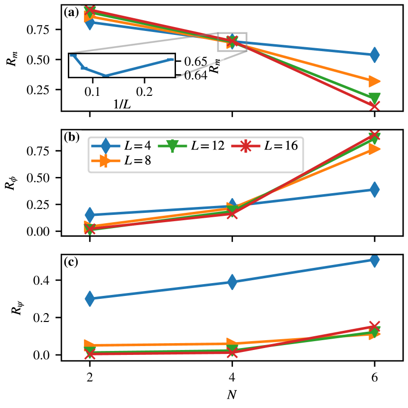
Figure 10: Correlation ratios of the staggered magnetization $m$ [Eq. (27)], $\phi$ [Eq. (28)] and $\psi$ [Eq. (29)] order parameters for $S=1/2$, as a function of $N$, and for lattice sizes $L=4-16$.

To obtain a reliable determination of the ground state, we study the correlation ratios of the three order parameters discussed in Sec. IV.1. In Fig. 10, we show the three correlation ratios $R_{m}$, $R_{\phi}$, and $R_{\psi}$ as a function of $N$, for lattice sizes $L=4,8,12,16$. The crossing plot of $R_{m}$ indicates the disappearance of Néel order at $N\approx 4$. At the same time, the curves of $R_{\phi}$ and $R_{\psi}$ exhibit a crossing for values of $N>4$; in particular, for $N=4$ both $R_{\phi}$ and $R_{\psi}$ decrease with the lattice size, indicating that both VBS and nematic order are short-ranged for $N=4$. Therefore, as anticipated above, for $N=4$ the ground state is still a Néel order. This confirms the result of Refs. [46, 47, 48]. At $N=6$, $R_{m}$ decreases with $L$, while $R_{\phi}$ and $R_{\psi}$ increases in $L$, for $L\geq 6$; the $L=4$ data set is dominated by finite-size effects. Accordingly, for $N=6$ the ground state realizes VBS order.

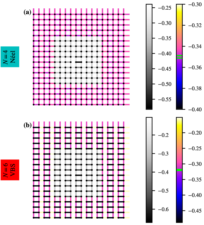
Figure 11: Real-space value of bonds $B_{i}(\boldsymbol{r})$ [Eq. (33)], as measured after pinning the central bond, for $S=1/2$ and lattice size $L=18$. Due to the observed different variations in the bond strength, in order to better highlight the patterns of bond correlations we have used different color scales for the region close and far from the pinned bond. The biggest error of the outer bonds is indicated by two red lines on the color scale. We have symmetrized the results with regards to inversions $y\rightarrow-y$, $x\rightarrow-x$ around the pinned bond.

These observations are confirmed by the real-space plot of the bond intensity shown in Fig. 11, as obtained with the pinning-field method. For $N=4$, in the vicinity of the pinned bond we observe a pattern reminiscent of the VBS order of Fig. 8. However, at larger distances the modulation of bond intensity quickly decays, confirming that VBS order is actually short ranged. For $N=6$, we observe a very clear pattern of strong and weak bonds that realize the VBS order.

IV.3 $S=1$

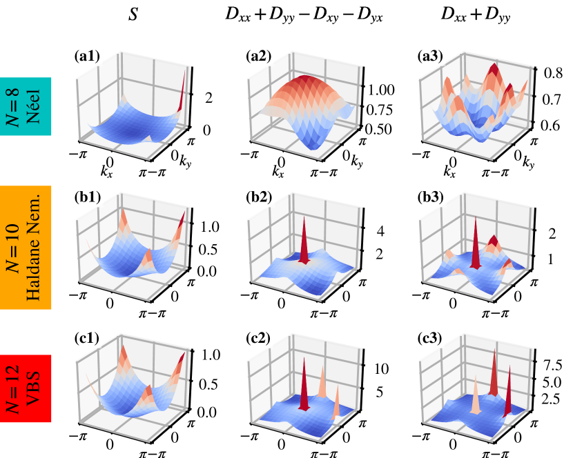
Figure 12: Same as Fig. 9 for $S=1$

In studying the representations with $S=1$, we proceed analogously to the $S=1/2$ case discussed in Sec. IV.2. In Fig. 12, we show the order parameters in momentum space for the case $S=1$, and three representative values of $N$. For $N=8$, a clear peak of the spin structure factor at $(\pi,\pi)$, along with a comparatively smoother momentum dependence of the other order parameters, indicate the presence of Néel order. At $N=10$, we observe instead the emergence of a clear signal of the nematic order parameter at zero momentum. The VBS order parameter exhibits a similar peak at zero momentum, whose signal predominantly arises from the nematic order parameter, while at momentum $(\pi,0)$ a subdominant peak is observed. The Néel order parameter instead does not show a predominant signal at $(\pi,\pi)$, but rather equally large values at the corners of the Brillouin zone. These behaviors suggest the onset of the two-fold degenerate nematic order. For $N=12$ a clear signal at $(\pi,0)$ momentum appears in the VBS order parameter. Along with the sharp zero-momentum value of the nematic order parameter, these findings suggest the realization of VBS order for $N=12$.

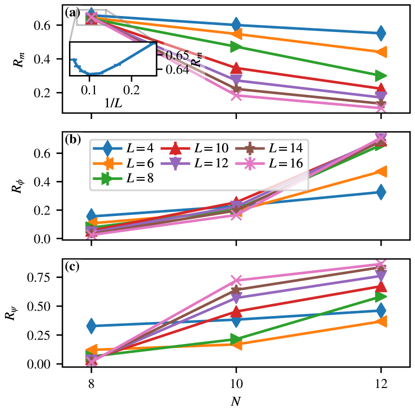
Figure 13: Same as Fig. 10 for $S=1$.

As we did for the $S=1/2$ case, the above qualitative observations on the momentum dependence of the various order parameters can be put on firm ground by examining the correlation ratios shown in Fig. 13. The magnetic correlation ratio $R_{m}$ displays a crossing at about $N\approx 8$, such that for $N>8$, $R_{m}$ decreases with the lattice size. On the other hand, at $N=8$ both $R_{\phi}$ and $R_{\psi}$ decrease on increasing $L$, implying that both VBS and nematic order are short ranged. Therefore, one can conclude that for $N=8$ the ground state is antiferromagnetically ordered. The behavior of $R_{\phi}$ shows rather important finite-size corrections. In fact, while curves for $L\leq 10$ cross for $8<N<10$, the crossing point quickly increases with $L$, such that for $L\geq 12$ a crossing is found for $10<N<12$. In particular, $N=10$ has a nonmonotonic behavior, increasing in $L$ for $L\leq 10$, and decreasing for $L\geq 12$. This observation supports the presence of a significant, but still short-ranged, VBS order, which is responsible for important finite-size corrections. The nematic correlation ratio $R_{\psi}$ shows a crossing between $N=8$ and $N=10$. Also, here we observe a clear drift in the crossing of $R_{\psi}$, although the situation for $N=10$ is rather clear and indicates long-range order in $\psi$. In view of these observations, and referring to Table 1, we conclude that a nematic ground state is realized for $N=10$, while for $N\geq 12$ the ground-state is VBS ordered.

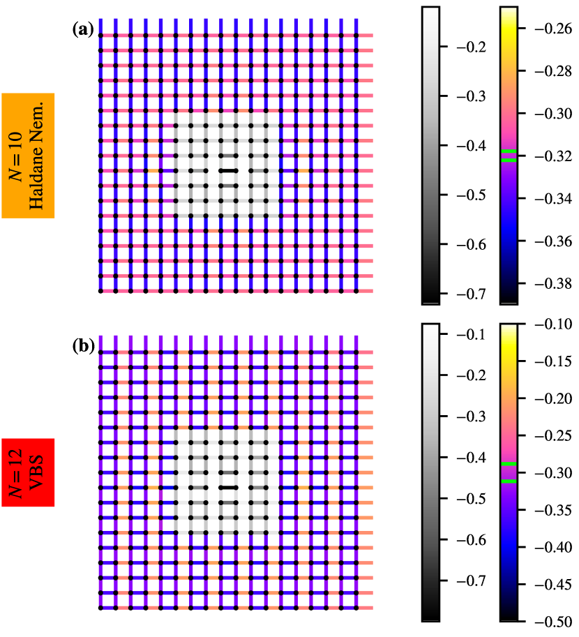
Figure 14: Same as Fig. 11 for $S=1$.

These conclusions are nicely confirmed by the real-space plots of the bond strength obtained with the pinning-field method and shown in Fig. 14. For $N=10$ we clearly observe the formation of a twofold degenerate stripe-like structure, signalling the presence of the nematic order. For $N=12$ instead a VBS order is found. Interestingly, while for $S=1/2$ the VBS order found at $N=6$ (Fig. 11) resembles the ladder order illustrated in Fig. 8, for $S=1$ and $N=12$ the VBS pattern shown in Fig. 14 rather suggests the plaquette order of Fig. 8.

IV.4 $S=3/2$

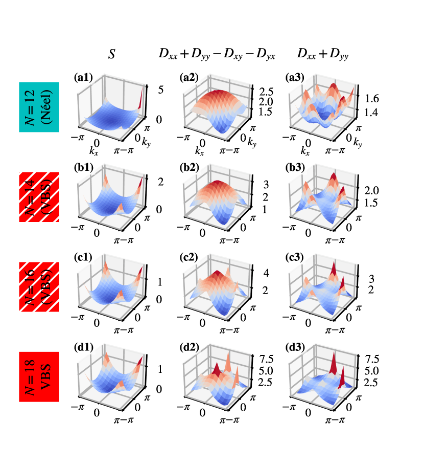
Figure 15: Same as Fig. 9 for $S=3/2$

In Fig. 15, we show the order parameters in momentum space, and $N=12-18$. Analogous to the cases analyzed in the previous sections, for $N=12$ we find a signal of Néel order. In the region $14\leq N\leq 16$, QMC data do not allow us to unambiguously single out the ground state. Upon increasing $N$, the peak at $(\pi,\pi)$ in $S(\boldsymbol{k})$ slowly decreases in magnitude. At the same time, we observe the appearance of a maximum in the nematic order parameter at zero momentum, and in the VBS order parameter for $(\pi,0)$ and $(0,\pi)$ momenta. Eventually, for $N=18$ the momentum structure of the order parameters more clearly favors the realization of VBS order. The observed behavior suggests a comparatively broad critical region around $14\leq N\leq 18$.

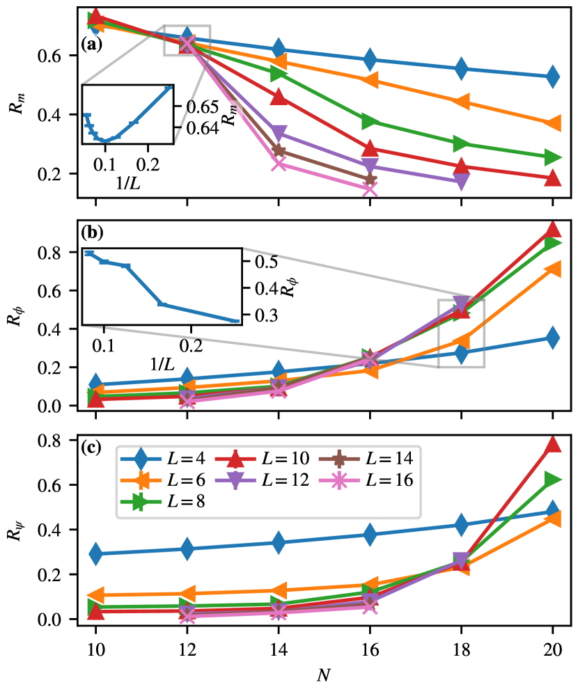
Figure 16: Same as Fig. 10 for $S=3/2$

In an attempt to better understand the ground-state diagram for $S=3/2$, as for the other values of $S$ we have analyzed the correlation ratios, shown in Fig. 16. Due to the increased computational costs, we restricted the simulations for the larger lattice sizes $L\geq 12$ to the more involved cases $12\leq N\leq 16$. For smaller lattice sizes $L\leq 10$, the curves for $R_{m}$ appear to cross at a value of $N$ very close, but smaller than $N<12$. We observe, however, some drift towards larger values of $N$ in the crossings. Furthermore, as shown in the inset of Fig. 16, $R_{m}$ at $N=12$ exhibits an upwards trend for $L>10$. Together with the observed slow decrease of $R_{\phi}$ and $R_{\psi}$ in $L$ for $N=12$, this implies Néel order for $N=12$.

For $N\geq 14$, the $L-$dependence of $R_{m}$ clearly rules out Néel order. On the other hand, $R_{\phi}$ slowly decreases with $L$ for $N=14$, and for $N=16$ it grows slightly up to $L=8$. In both cases, QMC data for $L\geq 8$ are indistinguishable within error bars. A similar flattening of QMC data is found in $R_{\psi}$ for $N=14,16$. This behavior does not allow us to draw firm conclusions on the nature of the ground state for $N=14,16$. Since a Néel state can be ruled out, a reasonable hypothesis is the realization of a VBS state, however, with a weak order parameter.

For $N>16$, both $R_{\phi}$ and $R_{\psi}$ show a crossing close to $N=18$. Furthermore, we observe a monotonic growth of $R_{\phi}$ in $L$ for $N=18$. This leads us to conclude a VBS order for $N=18$.

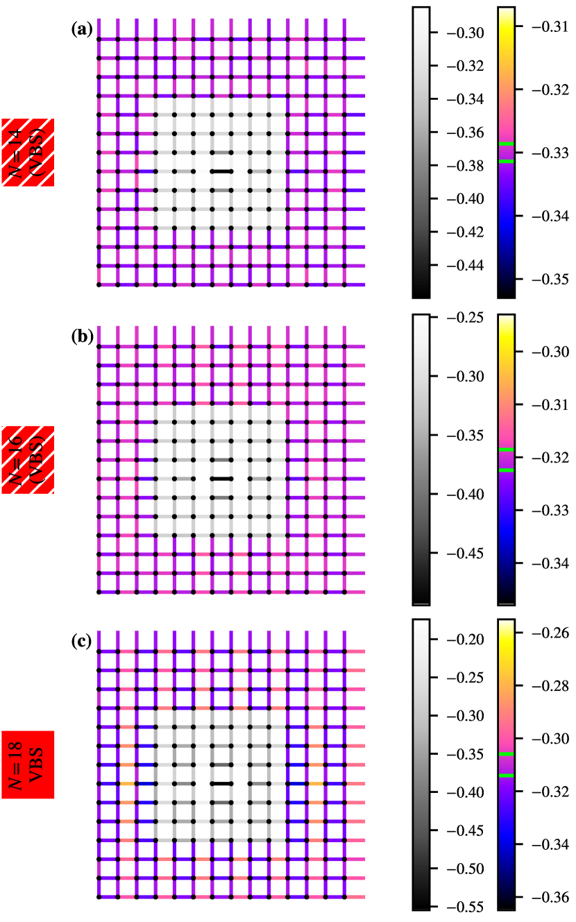
Figure 17: Same as Fig. 11 for $S=3/2$ and lattice size $L=14$ $(N=14,16)$, $L=12$ $(N=18)$.

Finally, we have studied the pattern of bond strength in real space with the pinning-field method. The results for $N=14,16,18$ are reported in Fig. 17. For $N=14,16$, despite some signs of dimerization, we do not observe a clear VBS pattern. In line with the previous analysis, for $N=18$ we find a bond dimerization which confirms a VBS ground state.

IV.5 $S=2$

As for previous values of $S$, we begin our investigation for $S=2$ with momentum space plots of correlation functions shown in Fig. 18. At $N=16$, the spin structure factor shows a sharp peak at $(\pi,\pi)$, indicating long-range AFM order. For bigger values of $N$ the peak weakens and broadens, suggesting short-range AFM order. The correlations for nematic and VBS order show only very broad maxima for the range $N\in[16,22]$, implying the absence of both of these orders. The correlation ratios plotted in Fig. 19 support these qualitative observations. The inset in Fig. 19(a) shows that while $R_{m}$ decreases at $N=16$ from $L=4$ to $L=12$, the trend is reversed on bigger lattices and $R_{m}$ increases from $L=12$ to $L=16$. This indicates that $N=16$ has a Néel ground state which is close to a competing order. Both $R_{\phi}$ and $R_{\psi}$ decrease with increasing system size in the investigated range $N\in[16,24]$. As per Table 1, this leaves a two-dimensional AKLT order as a ground-state candidate for $N\in[18,24]$. With the AKLT construction corresponding to the right-hand side of Fig. 8(e), we understand that each boundary site hosts an $\mathfrak{su}(N)$ representation corresponding to one column ($S=1/2$) and $N/2$ rows. Hence the boundary defines a one-dimensional chain in the aforementioned representation. It is known that for $N\geq 4$ this chain dimerizes [49, 50, 46, 47].

To further investigate this possibility, we simulate the model on a lattice with periodic boundary conditions in the $x$ direction and open boundary conditions along $y$, corresponding to a cylinder geometry. Fig. 20 shows the results for $S=2,N=18$ in a pinning-field approach with pinned bonds at the edge and in the bulk, respectively. The induced dimerization pattern propagates on the edge much further than in the bulk, supporting the presence of an AKLT phase with boundary corresponding to an $S=1/2$ $\text{SU}(N)$ chain in the totally antisymmetric self-adjoint representation.

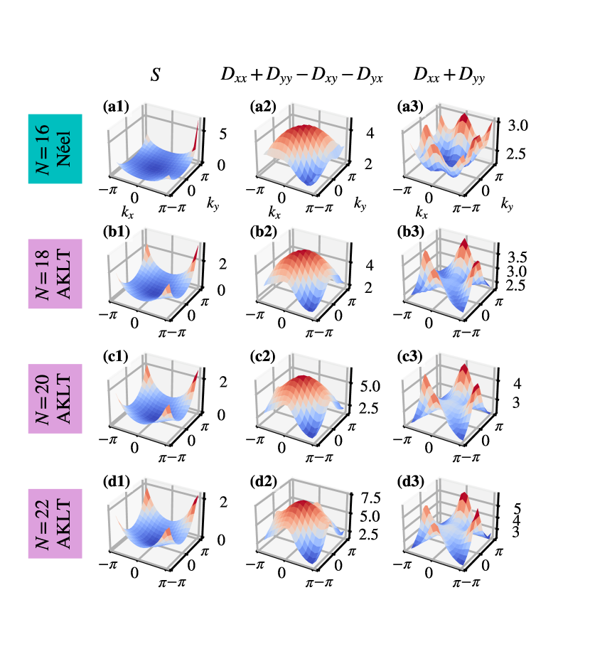
Figure 18: Same as Fig. 9 for $S=2$

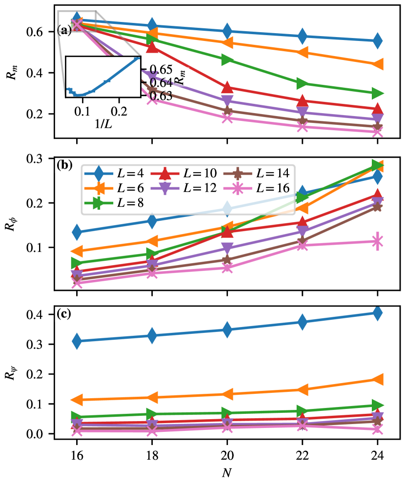
Figure 19: Same as Fig. 10 for $S=2$

Figure 20: Real-space value of bonds $B_{i}(\boldsymbol{r})$ for $S=2$, $N=18$, lattice size $L\in\{8,10,12\}$ and open boundary conditions in $y$ direction. Comparison between pinning a bond at the edge (a) and a bond in the bulk (b). (c) $B_{\rm x}(\boldsymbol{r})$ on horizontal lines through the pinned bonds.

V Summary

We have studied the ground-state phase diagram of an $\text{SU}(N)$ AFM model on the square lattice, with irreducible representations of $\mathfrak{su}(N)$ illustrated in Fig. 2 and characterized by a Young tableau consisting of $2S$ columns and $N/2$ rows. For even values of $N$ we have presented negative sign free QMC data that results in the rich phase diagram of Fig. 1. In line with field-theoretical studies [22, 23, 24], for any value of the generalized spin $S$, we found Néel order at small values of $N$, and a dimerized VBS state for large $N$. The disordered states proximate to the melting of the Néel state can be naturally understood in terms of condensation of monopoles. These states turn out to be located along the line $N=8S+2$ in the $S$ versus $N$ phase diagram. At $S=1$ we observe nematic AKLT [40] states where $C_{4}$ symmetry is spontaneously reduced to $C_{2}$, with the emergence of spin-1 chains along one lattice direction. At $S=2$, the AKLT construction provides an understanding of the non-degenerate state. In fact, this construction can be generalized to any spin $S=Z/2$ system on a lattice with coordination number $Z$; an example for the honeycomb lattice is given in Refs. [51, 52]. In our specific case, the edge state corresponds to an $\text{SU}(N)$ spin system in an irreducible representation specified by a Young tableau with one column ($S=1/2$) and $N/2$ rows. At $N\geq 4$, such a state is know to dimerize [47]. Our simulations with open boundary conditions support this picture. For half-integer values of $S$, a four fold degenerate VBS state emerges. The detailed nature of the dimerization was studied using a pinning-field approach [44].

While the resulting phase diagram reproduced in Fig. 1 will serve as a benchmark for future studies, our findings points to future avenues of research. It would be very interesting to study in detail the quantum phase transitions between the various states. Although the present setup allows us to consider integer values of $N$ only, it may be possible to investigate the phase transitions with a suitably defined designer Hamiltonian containing, e.g., some interactions that favor a specific phase, so as to be able to interpolate between them. The topological arguments that lead to the observed phase diagram carry over to other representation of $\mathfrak{su}(N)$  such that further calculations with alternative methods such as stochastic series expansion [53] are certainly desirable.

Appendix A The quadratic Casimir eigenvalue in terms of the Young tableau

In this appendix, we discuss the relation between the Young tableau of an irreducible representation and the corresponding eigenvalue of the quadratic Casimir operator. For an irreducible representation, whose Young tableau has $n_{l}$ rows of length $\{l_{i}\}$ and $n_{c}$ columns of length $\{c_{i}\}$, the eigenvalue of the quadratic Casimir operator is [38]

$$C=\frac{1}{2}\left[r\left(N-\frac{r}{N}\right)+\sum_{i}^{n_{l}}l_{i}^{2}-\sum_{i}^{n_{c}}c_{i}^{2}\right],$$ (35)

where $r=\sum_{i}l_{i}=\sum_{i}c_{i}$ is the total number of boxes.

In this appendix, we also derive Eq. (35), which is stated in the Appendix of Ref. [38] without an explicit proof. First, we notice that in Eq. (35) there is an implicit choice of normalization. As we show below, such a normalization is consistent with Eq. (10).

For an irreducible representation, the value of $C$ can be easily computed with Weyl’s formula [31, 54],

$$C=\langle\Lambda|\Lambda+2\delta\rangle,$$ (36)

where $\Lambda$ is the maximum weight of the representation and $\delta$ the Weyl vector. In the Dynkin representation the metric tensor of the scalar product is, up to a normalization $\cal N$, the inverse of the transpose of the Cartan matrix $A$ [31],

$$\begin{split}G^{ij}&={\cal N}\left[\left(A^{T}\right)^{-1}\right]_{ij},\\ \left[\left(A^{T}\right)^{-1}\right]_{ij}&=\text{min}(i,j)-\frac{ij}{N},\end{split}$$ (37)

and the Weyl vector is $\delta=(1,1,\ldots,1)$. To fix the normalization ${\cal N}$, we compute $C$ for the defining representation, and match it with Eq. (10). For the defining representation, the maximum Dynkin weight is $\Lambda_{\alpha_{i}}=\delta_{i,1}$, hence

$$\begin{split}C&={\cal N}\sum_{i,j=1}^{N-1}\delta_{i,1}\left[\text{min}(i,j)-\frac{ij}{N}\right]\left(\delta_{j,1}+2\right)\\ &={\cal N}\frac{N^{2}-1}{N}.\end{split}$$ (38)

On the other hand, by taking the trace on both hand sides of Eq. (10), $C$ is readily computed as $C=(N^{2}-1)/(2N)$. Therefore the normalization constant is ${\cal N}=1/2$.

Employing Eq. (36), we first compute $\langle\Lambda|\Lambda\rangle$. Using Eq. (2)

$$\langle\Lambda|\Lambda\rangle=\sum_{i,j=1}^{N-1}\left(l_{i}-l_{i+1}\right)G^{ij}\left(l_{j}-l_{j+1}\right),$$ (39)

where the metric tensor $G^{ij}$ is given in Eq. (37). By developing the products and employing change of variables $i\rightarrow i-1$, $j\rightarrow j-1$, Eq. (39) can be written as

$$\begin{split}\langle\Lambda|\Lambda\rangle=&l_{1}G^{11}l_{1}\\ &+l_{1}\sum_{j=2}^{N-1}\left(G^{1,j}-G^{1,j-1}\right)l_{j}\\ &+\sum_{i=2}^{N-1}l_{i}\left(G^{i,1}-G^{i-1,1}\right)l_{1}\\ &+\sum_{i,j=2}^{N-1}l_{i}\left(G^{i,j}-G^{i-1,j}-G^{i,j-1}+G^{i-1,j-1}\right)l_{j},\end{split}$$ (40)

where we have used that $l_{N}=0$ for Young tableaux of $\mathfrak{su}(N)$ representations. Using Eq. (37), we have

$$G^{1,j}-G^{1,j-1}=G^{i,1}-G^{i-1,1}=-\frac{1}{2N},$$ (41)

where we have employed the normalization ${\cal N}=1/2$ obtained after Eq. (38). Further, using Eq. (37), the difference in the parenthesis in the last term of Eq. (40) is computed as

$$\begin{split}&G^{i,j}-G^{i-1,j}-G^{i,j-1}+G^{i-1,j-1}=\\ &\frac{1}{2}\Big{[}\text{min}(i,j)-\text{min}(i-1,j)\\ &-\text{min}(i,j-1)-\text{min}(i-1,j-1)-\frac{1}{N}\Big{]}.\end{split}$$ (42)

By enumerating the various cases, it is easy to see that

$$\text{min}(i,j)-\text{min}(i-1,j)-\text{min}(i,j-1)-\text{min}(i-1,j-1)=\delta_{ij}.$$ (43)

Using Eqs. (41), (42) and (43) in Eq. (40), we obtain the first term in Weyl’s formula,

$$\begin{split}\langle\Lambda|\Lambda\rangle=&\frac{l_{1}^{2}}{2}\left(1-\frac{1}{N}\right)-\frac{1}{N}l_{1}\left(r-l_{1}\right)\\ &+\frac{1}{2}\sum_{i=1}^{N-1}l_{i}^{2}-\frac{1}{2}l_{1}^{2}+\frac{1}{2N}\left(r-l_{1}\right)^{2}\\ =&\frac{1}{2}\left(\sum_{i=1}^{n_{l}}l_{i}^{2}-\frac{r^{2}}{N}\right),\end{split}$$ (44)

where $r=\sum_{i}l_{i}$ is the total number of boxes and the sum over $l_{i}^{2}$ can be restricted to the $n_{l}$ nonzero row lengths.

To compute the second term $\langle\Lambda|2\delta\rangle$ in Weyl’s formula, we use a different parametrization of $\Lambda$. Since in the Dynkin representation the components of $\Lambda_{\alpha_{i}}$ are positive integers [see Eq. (2)], we can parametrize $\Lambda_{\alpha_{i}}$ as

$$\Lambda_{\alpha_{i}}=\sum_{a=1}^{n_{c}}\delta_{i,c_{a}}.$$ (45)

The set $\{c_{a}\}$ represents the position of the rows in the corresponding Young tableau where the number of boxes decreases on the following row. Such a decrease corresponds to the end of the column, hence $\{c_{a}\}$ are the column lengths. Using Eqs. (45) and (37) we have

$$\begin{split}\langle\Lambda|2\delta\rangle&=\frac{1}{2}\sum_{i,j=1}^{N-1}\sum_{a,b=1}^{n_{c}}\left(\delta_{i,c_{a}}\text{min}(i,j)2-\delta_{i,c_{a}}\frac{ij}{N}2\right)\\ &=\sum_{a=1}^{n_{c}}\sum_{j=1}^{N-1}\text{min}(c_{a},j)-\sum_{a=1}^{n_{c}}\sum_{j=1}^{N-1}\frac{c_{a}j}{N}\end{split}$$ (46)

The first sum in Eq. (46) can be written as

$$\begin{split}\sum_{a=1}^{n_{c}}\sum_{j=1}^{N-1}\text{min}(c_{a},j)&=\sum_{a=1}^{n_{c}}\left(\sum_{j=1}^{c_{a}}j+\sum_{j=c_{a}+1}^{N-1}c_{a}\right)\\ &=\left(N-\frac{1}{2}\right)r-\frac{1}{2}\sum_{a=1}^{n_{c}}c_{a}^{2},\end{split}$$ (47)

where we have used $\sum_{a}c_{a}=r$. The second sum in Eq. (46) can be computed as

$$\sum_{a=1}^{n_{c}}\sum_{j=1}^{N-1}\frac{c_{a}j}{N}=\frac{1}{2}r(N-1)$$ (48)

Inserting Eqs. (47) and (48) in Eq. (46), we obtain the second term of Weyl’s formula

$$\langle\Lambda|2\delta\rangle=\frac{1}{2}\left(rN-\sum_{a=1}^{n_{c}}c_{a}^{2}\right).$$ (49)

Finally, employing Eqs. (44) and (49) in Eq. (36) one obtains Eq. (35).

As is known from the rules of Young tableaux of $\mathfrak{su}(N)$ representations, columns of length $N$ can be deleted since they correspond to an invariant under $\text{SU}(N)$. This is consistent with the formula of Eq. (35). Indeed, by adding to a Young tableau a column of length $N$, we have

$$\begin{split}r&\rightarrow r+N,\\ l_{i}&\rightarrow l_{i}+1,\\ \sum_{i=1}^{n_{c}}c_{i}^{2}&\rightarrow N^{2}+\sum_{i=1}^{n_{c}}c_{i}^{2}.\end{split}$$ (50)

Inserting the substitutions of Eq. (50) in Eq. (35), one can check that the Casimir eigenvalue is left unchanged.

Finally, it is easy to check that in the case of the defining representation, whose Young tableau is a single box, Eq. (35) gives the expected result, with the normalization consistent with Eq. (10).

Appendix B Bound on the eigenvalue of the quadratic Casimir operator

The tensor product of $2S$ self-adjoint antisymmetric representations given in Eq. (16) decomposes into different irreducible representations. In this appendix we prove that among those representations, the maximally symmetric one of Fig. 2 has the maximum Casimir eigenvalue, which we compute.

Due to the rules for the composition of Young tableaux, each of the irreducible representations arising from the tensor product has a Young tableau whose total number of boxes is $r\leq(2S)(N/2)=NS$ and whose row lengths cannot exceed $2S$, $l_{i}\leq 2S$. Thus an upper bound for $\sum_{i}l_{i}^{2}$ appearing in Eq. (35) is

$$\sum_{i}^{n_{l}}l_{i}^{2}\leq\sum_{i}^{n_{l}}2Sl_{i}=2Sr.$$ (51)

This bound is saturated by

$$l_{i}=2S,\qquad n_{l}=r/(2S).$$ (52)

On the other hand, an upper bound for the second sum in Eq. (35) is found using the Cauchy-Schwartz inequality on the $n_{c}-$component vectors $(c_{1},\ldots,c_{n})$ and $(1,\ldots,1)$:

$$(c_{1}^{2}+\ldots+c_{n}^{2})(1+\ldots+1)\geq(c_{1}+\ldots+c_{n})^{2}.$$ (53)

The number of columns in the Young tableau $n_{c}$ is bounded by $n_{c}=\text{max}(\{l_{i}\})\leq 2S$, and their sum is $\sum c_{i}=r$. Hence, Eq. (53) gives

$$\sum_{i}^{n_{c}}c_{i}^{2}\geq\frac{r^{2}}{n_{c}}\geq\frac{r^{2}}{2S}.$$ (54)

This bound is saturated by

$$c_{i}=r/(2S),\qquad n_{c}=2S.$$ (55)

Inserting Eqs. (51) and (54) in Eq. (35) we get

$$C\leq\frac{N+2S}{2}\left(-\frac{r^{2}}{2SN}+r\right)\leq\frac{NS(2S+N)}{4},$$ (56)

where the upper bound is obtained for $r=NS$. Together with Eqs. (52) and (55), this precisely corresponds to the Young tableau of Fig. 2. Its Casimir eigenvalue is most easily computed using Weyl’s formula [Eq. (36)] and Eq. (3), obtaining Eq. (22), which saturates the upper bound of Eq. (56). Alternatively, the Casimir eigenvalue can be obtained from Eq. (35), and $r=NS$, $l_{1}=l_{2}=\ldots=l_{N/2}=2S$ and $c_{1}=c_{2}=\ldots=c_{2S}=N/2$.

Finally, we observe that, since the variables $\{l_{i}\}$ and $\{c_{i}\}$ in Eq. (35) are positive integers, as soon as we deviate from the solution maximizing $C$, we decrease the Casimir eigenvalue by a finite integer amount. In other words, there is a finite gap $O(1)$ in the eigenvalues of the quadratic Casimir operators between the subspace of the representation of Fig. 2 and the other irreducible representations arising from the tensor product of $2S$ self-adjoint antisymmetric representations.

Appendix C Systematic errors

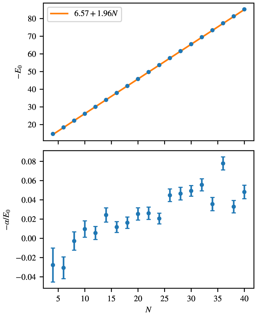
Figure 21: Scaling of systematic $\Delta_{\tau}$ error for $L=4$, $\Theta=2$, and $S=1/2$. For each point, we simulated with a range of different values for $\Delta\tau$ and fitted the energy to $E(\Delta_{\tau})=E_{0}+\alpha{\Delta_{\tau}}^{2}$.

In this appendix we show that there is no explicit dependence on the magnitude of the Trotter error as a function of $N$. To keep the notation simple, we will show this on the basis of the $S=1/2$ Hamiltonian where $\hat{H}_{\text{Casimir}}$ [see Eq. 19] as well as the orbital index can be omitted:

$$\begin{split}\hat{H}_{\text{QMC}}=&\hat{H}_{J}+\hat{H}_{U}\\ =&-\frac{J}{2N}\sum_{\langle i,j\rangle}\left\{\hat{D}_{i,j},\hat{D}^{\dagger}_{i,,j}\right\}+\frac{U}{N}\sum_{i}\left(\hat{n}_{i}-\frac{N}{2}\right)^{2}\end{split}$$ (57)

In this appendix, we have normalized the Hamiltonian by the factor $\frac{1}{N}$, such that total energy differences defining, e.g., the spin gap [$E_{0}(S=1)-E_{0}$] remain constant in the large-$N$ limit. In particular, with the mean-field ansatz $\chi_{i,j}=\frac{1}{N}\langle\hat{D}_{i,j}\rangle$ corresponding to the Affleck and Marston saddle point [55], the Hamiltonian reads:

$$\hat{H}_{\text{MF}}=-\frac{J}{2}\sum_{\langle i,j\rangle}\chi_{i,j}\hat{D}^{\dagger}_{i,,j}+\overline{\chi_{i,j}}\hat{D}_{i,,j}.$$ (58)

In this large-$N$ limit, one will check explicitly that the spin gap on a finite lattice is $N$ independent, and that the energy is extensive in the volume, $V$, and in $N$. Since gaps are $N$ independent, at least in the large-$N$ limit, it makes sense comparing results at different $N$ but at constant temperature or projection parameter.

In the formulation of the AF QMC method, one introduces a checkerboard decomposition, where the interaction terms are grouped into disjoint families of commuting operators. This factorization introduces a Trotter discretization error, whose $N-$dependence we estimate as follows. To render the calculation as simple as possible, we will consider as an illustration a one-dimensional chain. In this case, the checkerboard decomposition in even and odd bonds, $b$, allows us to write the Hamiltonian as:

$$\hat{H}=\underbrace{\sum_{b\in A}\hat{h}_{b}}_{\equiv\hat{H}_{A}}+\underbrace{\sum_{b\in B}\hat{h}_{b}}_{\equiv\hat{H}_{B}}.$$ (59)

Both $\hat{H}_{A}$ and $\hat{H}_{B}$ are sums of commuting terms. $\hat{h}_{b}$ corresponds to a local Hamiltonian, such that it is extensive in $N$ but intensive in volume.

An explicit form of $\hat{h}_{b}$ on a bond with legs $i$,$j$ in the fermion representation would read: $\frac{1}{N}\left\{\hat{D}_{(i,j)},\hat{D}^{\dagger}_{(i,j)}\right\}$. Note that to keep calculations as simple as possible we, implicitly consider a one-dimensional lattice in which $\hat{H}_{A}$ is a sum of commuting terms. For the two-dimensional case, the checkerboard bond decomposition necessitates four terms. We will use the symmetric Trotter decomposition,

$$e^{-\Delta\tau\hat{H}+\Delta\tau^{3}\hat{R}_{3}}=e^{-\frac{\Delta\tau}{2}\hat{H}_{A}}e^{-\Delta\tau\hat{H}_{B}}e^{-\frac{\Delta\tau}{2}\hat{H}_{A}}+{\cal O}\left(\Delta\tau^{5}\right)$$ (60)

with $\hat{R}_{3}=\left(\left[\hat{H}_{A},\left[\hat{H}_{A},\hat{H}_{B}\right]\right]+2\left[\hat{H}_{B},\left[\hat{H}_{B},\hat{H}_{A}\right]\right]\right)/24$. Since $\hat{H}_{A}$ and $\hat{H}_{B}$ are sums of local operators, $\hat{R}_{3}$ is also a sum of local operators. Hence, $\hat{R}_{3}$ is extensive in the volume. By explicitly computing the commutators, one will also show, that $\hat{R}_{3}$ is extensive in $N$. Hence $\hat{R}_{3}$ scales as $\hat{H}$. Note that for non-local Hamiltonians considered in Ref. [56], this does not apply. We can now compute the corrections to the free energy:

$$F_{\text{QMC}}=F-\Delta\tau^{2}\frac{\text{Tr}e^{-\beta\hat{H}}\hat{R}_{3}}{\text{Tr}e^{-\beta\hat{H}}}+{\cal O}(\Delta\tau^{4}).$$ (61)

Hence the quantity plotted in Fig. 21 corresponds to

$$\langle\hat{R}_{3}\rangle/\langle\hat{H}\rangle.$$ (62)

It is intensive in $N$ and $V$, such that it has a well defined value in the large-$N$ limit.

Appendix D Bounds on the bond observable

In this appendix, we discuss a lower and upper bound for a bond observable $\sum_{a}\hat{S}^{(a)}_{i}\hat{S}^{(a)}_{j}$, where $i$ and $j$ are two distinct lattice sites, not necessarily nearest neighbor. The bond observable can be expressed as

$$\sum_{a}\hat{S}^{(a)}_{i}\hat{S}^{(a)}_{j}=\frac{1}{2}\sum_{a}\left(\hat{S}^{(a)}_{i}+\hat{S}^{(a)}_{j}\right)\left(\hat{S}^{(a)}_{i}+\hat{S}^{(a)}_{j}\right)\\ -\frac{1}{2}\sum_{a}\hat{S}^{(a)}_{i}\hat{S}^{(a)}_{i}-\frac{1}{2}\sum_{a}\hat{S}^{(a)}_{j}\hat{S}^{(a)}_{j}.$$ (63)

With the choice of Eq. (9), the first term on the right-hand side of Eq. (63) is the quadratic Casimir element $\hat{C}_{2,\Gamma_{i}\otimes\Gamma_{j}}$ of the tensor product of the two $\mathfrak{su}(N)$ representations $\Gamma_{i}$ and $\Gamma_{j}$, at lattice sites $i$ and $j$ [compare with Eq. (10)]. The spectrum of $\hat{C}_{2,\Gamma_{i}\otimes\Gamma_{j}}$ consists in the eigenvalues of the quadratic Casimir operator of all irreducible representations to which $\Gamma_{i}\otimes\Gamma_{j}$ reduces. An upper bound is readily found by the maximally symmetric composition of $\Gamma_{i}$ and $\Gamma_{j}$, which corresponds to a Young tableau with $N/2$ rows and $4S$ columns; the proof is identical to that of Appendix B. Being a square of a hermitian operator, $\hat{C}_{2,\Gamma_{i}\otimes\Gamma_{j}}\geq 0$. Such lower bound is saturated by the totally antisymmetric composition of $\Gamma_{i}$ and $\Gamma_{j}$, which corresponds to the trivial $S=0$ representation. The second and third term on the right-hand side of Eq. (63) are the quadratic Casimir operators of the $\mathfrak{su}(N)$ representation considered here, and take the value given in Eq. (22). Inserting the bounds on $\hat{C}_{2,\Gamma_{i}\otimes\Gamma_{j}}$ discussed above in Eq. (63), we obtain

$$-C(N,S)\leq\Braket{\sum_{a}\hat{S}^{(a)}_{i}\hat{S}^{(a)}_{j}}\\ \leq C(N,2S)/2-C(N,S)=\frac{NS^{2}}{2}.$$ (64)

References

- Onsager [1944] L. Onsager, Crystal statistics. i. a two-dimensional model with an order-disorder transition, Phys. Rev. 65, 117 (1944).
- Sachdev [2011] S. Sachdev, Quantum Phase Transitions, 2nd ed. (Cambridge University Press, 2011).
- Diep [2020] H. T. Diep, Frustrated Spin Systems, 3rd ed. (World Scientific, 2020).
- Castelnovo et al. [2012] C. Castelnovo, R. Moessner, and S. Sondhi, Spin ice, fractionalization, and topological order, Annual Review of Condensed Matter Physics 3, 35 (2012), https://doi.org/10.1146/annurev-conmatphys-020911-125058 .
- Balents [2010] L. Balents, Spin liquids in frustrated magnets, Nature 464, 199 (2010).
- Senthil et al. [2004] T. Senthil, A. Vishwanath, L. Balents, S. Sachdev, and M. P. A. Fisher, Deconfined quantum critical points, Science 303, 1490 (2004).
- Nishimori [2001] H. Nishimori, Statistical Physics of Spin Glasses and Information Processing: An Introduction, International series of monographs on physics (Oxford University Press, 2001).
- Nielsen and Chuang [2010] M. Nielsen and I. Chuang, Quantum Computation and Quantum Information: 10th Anniversary Edition (Cambridge University Press, 2010).
- Sandvik [1997] A. W. Sandvik, Finite-size scaling of the ground-state parameters of the two-dimensional heisenberg model, Phys. Rev. B 56, 11678 (1997).
- Calandra Buonaura and Sorella [1998] M. Calandra Buonaura and S. Sorella, Numerical study of the two-dimensional heisenberg model using a green function monte carlo technique with a fixed number of walkers, Phys. Rev. B 57, 11446 (1998).
- Coldea et al. [2001] R. Coldea, S. M. Hayden, G. Aeppli, T. G. Perring, C. D. Frost, T. E. Mason, S.-W. Cheong, and Z. Fisk, Spin waves and electronic interactions in , Phys. Rev. Lett. 86, 5377 (2001).
- Zaliznyak et al. [1994] I. A. Zaliznyak, L.-P. Regnault, and D. Petitgrand, Neutron-scattering study of the dynamic spin correlations in above néel ordering, Phys. Rev. B 50, 15824 (1994).
- Kugel’ and Khomskiĭ [1982] K. I. Kugel’ and D. I. Khomskiĭ, The jahn-teller effect and magnetism: transition metal compounds, Soviet Physics Uspekhi 25, 231 (1982).
- Kugel et al. [2015] K. I. Kugel, D. I. Khomskii, A. O. Sboychakov, and S. V. Streltsov, Spin-orbital interaction for face-sharing octahedra: Realization of a highly symmetric su(4) model, Phys. Rev. B 91, 155125 (2015).
- Nakatsuji et al. [2012] S. Nakatsuji, K. Kuga, K. Kimura, R. Satake, N. Katayama, E. Nishibori, H. Sawa, R. Ishii, M. Hagiwara, F. Bridges, T. U. Ito, W. Higemoto, Y. Karaki, M. Halim, A. A. Nugroho, J. A. Rodriguez-Rivera, M. A. Green, and C. Broholm, Spin-orbital short-range order on a honeycomb-based lattice, Science 336, 559 (2012), http://science.sciencemag.org/content/336/6081/559.full.pdf .
- Corboz et al. [2012] P. Corboz, M. Lajkó, A. M. Läuchli, K. Penc, and F. Mila, Spin-orbital quantum liquid on the honeycomb lattice, Phys. Rev. X 2, 041013 (2012).
- Wu et al. [2003] C. Wu, J. P. Hu, and S. C. Zhang, Exact so(5) symmetry in the spin-3/2 fermionic system, Phys. Rev. Lett. 91, 186402 (2003).
- Gorshkov et al. [2010] A. V. Gorshkov, M. Hermele, V. Gurarie, C. Xu, P. S. Julienne, J. Ye, P. Zoller, E. Demler, M. D. Lukin, and A. M. Rey, Two-orbital su(n) magnetism with ultracold alkaline-earth atoms, Nat. Phys. 6, 289 (2010).
- Haldane [1983] F. D. M. Haldane, Nonlinear field theory of large-spin heisenberg antiferromagnets: Semiclassically quantized solitons of the one-dimensional easy-axis néel state, Phys. Rev. Lett. 50, 1153 (1983).
- Haldane [1988] F. D. M. Haldane, O(3) nonlinear model and the topological distinction between integer- and half-integer-spin antiferromagnets in two dimensions, Phys. Rev. Lett. 61, 1029 (1988).
- Sandvik [2007] A. W. Sandvik, Evidence for deconfined quantum criticality in a two-dimensional heisenberg model with four-spin interactions, Phys. Rev. Lett. 98, 227202 (2007).
- Read and Sachdev [1989a] N. Read and S. Sachdev, Some features of the phase diagram of the square lattice su(n) antiferromagnet, Nucl. Phys. B 316, 609 (1989a).
- Read and Sachdev [1989b] N. Read and S. Sachdev, Valence-bond and spin-peierls ground states of low-dimensional quantum antiferromagnets, Phys. Rev. Lett. 62, 1694 (1989b).
- Read and Sachdev [1990] N. Read and S. Sachdev, Spin-peierls, valence-bond solid, and néel ground states of low-dimensional quantum antiferromagnets, Phys. Rev. B 42, 4568 (1990).
- Blankenbecler et al. [1981] R. Blankenbecler, D. J. Scalapino, and R. L. Sugar, Monte Carlo calculations of coupled boson-fermion systems. I, Phys. Rev. D 24, 2278 (1981).
- White et al. [1989] S. R. White, D. J. Scalapino, R. L. Sugar, E. Y. Loh, J. E. Gubernatis, and R. T. Scalettar, Numerical study of the two-dimensional Hubbard model, Phys. Rev. B 40, 506 (1989).
- Sorella et al. [1989] S. Sorella, S. Baroni, R. Car, and M. Parrinello, A novel technique for the simulation of interacting fermion systems, Europhysics Letters (EPL) 8, 663 (1989).
- Assaad and Evertz [2008] F. F. Assaad and H. Evertz, World-line and Determinantal Quantum Monte Carlo Methods for Spins, Phonons and Electrons, in Computational Many-Particle Physics, Lecture Notes in Physics, Vol. 739, edited by H. Fehske, R. Schneider, and A. Weiße (Springer, Berlin, 2008) pp. 277–356.
- Assaad et al. [2022] F. F. Assaad, M. Bercx, F. Goth, A. Götz, J. S. Hofmann, E. Huffman, Z. Liu, F. P. Toldin, J. S. E. Portela, and J. Schwab, The ALF (Algorithms for Lattice Fermions) project release 2.0. Documentation for the auxiliary-field quantum Monte Carlo code, SciPost Phys. Codebases , 1 (2022).
- Assaad [2005] F. F. Assaad, Phase diagram of the half-filled two-dimensional hubbard-heisenberg model: A quantum monte carlo study, Phys. Rev. B 71, 075103 (2005).
- Vergados [2017] J. D. Vergados, Group and Representation Theory (World Scientific, 2017).
- Note [1] In Eq. (1) and Eq. (8) we have implicitly assumed a choice of the basis of , such that the interaction term is -invariant. This condition is satisfied by the basis choice given below in Eq. (9).
- Note [2] We notice that the operator defined in Eq. (10) commutes with the algebra only for completely antisymmetric structure constants. For a general choice of the base, one needs to introduce a metric tensor determined by the structure constants and the Casimir operator is defined as [31]; for completely antisymmetric structure constants . Also, for the same reason, a normalization is implicit in the definition of Eq. (10), discussed in App. A.
- Sugiyama and Koonin [1986] G. Sugiyama and S. Koonin, Auxiliary field monte-carlo for quantum many-body ground states, Annals of Physics 168, 1 (1986).
- Wang et al. [2017] Z. Wang, F. F. Assaad, and F. Parisen Toldin, Finite-size effects in canonical and grand-canonical quantum Monte Carlo simulations for fermions, Phys. Rev. E 96, 042131 (2017), arXiv:1706.01874 [cond-mat.stat-mech] .
- Shen et al. [2020] T. Shen, Y. Liu, Y. Yu, and B. M. Rubenstein, Finite temperature auxiliary field quantum monte carlo in the canonical ensemble, J. Chem. Phys. 153, 204108 (2020), arXiv:2010.09813 [quant-ph] .
- Haber [2021] H. E. Haber, Useful relations among the generators in the defining and adjoint representations of SU(N), SciPost Phys. Lect. Notes 21, arXiv:1912.13302 (2021), arXiv:1912.13302 [math-ph] .
- Pilch and Schellekens [1984] K. Pilch and A. N. Schellekens, Formulas for the eigenvalues of the Laplacian on tensor harmonics on symmetric coset spaces, J. Mat. Phys. 25, 3455 (1984).
- Bercx et al. [2017] M. Bercx, F. Goth, J. S. Hofmann, and F. F. Assaad, The ALF (Algorithms for Lattice Fermions) project release 1.0. Documentation for the auxiliary field quantum Monte Carlo code, SciPost Phys. 3, 013 (2017), arXiv:1704.00131 [cond-mat.str-el] .
- Affleck et al. [1988] I. Affleck, T. Kennedy, E. H. Lieb, and H. Tasaki, Valence bond ground states in isotropic quantum antiferromagnets, Commun. Math. Phys. 115, 477 (1988).
- Desai and Kaul [2019] N. Desai and R. K. Kaul, Spin-s designer hamiltonians and the square lattice s =1 haldane nematic, Phys. Rev. Lett. 123, 107202 (2019), arXiv:1904.09629 [cond-mat.str-el] .
- Caracciolo and Pelissetto [1998] S. Caracciolo and A. Pelissetto, Corrections to finite-size scaling in the lattice N-vector model for N=, Phys. Rev. D 58, 105007 (1998), hep-lat/9804001 .
- Parisen Toldin et al. [2015] F. Parisen Toldin, M. Hohenadler, F. F. Assaad, and I. F. Herbut, Fermionic quantum criticality in honeycomb and -flux Hubbard models: Finite-size scaling of renormalization-group-invariant observables from quantum Monte Carlo, Phys. Rev. B 91, 165108 (2015), arXiv:1411.2502 [cond-mat.str-el] .
- Assaad and Herbut [2013] F. F. Assaad and I. F. Herbut, Pinning the Order: The Nature of Quantum Criticality in the Hubbard Model on Honeycomb Lattice, Phys. Rev. X 3, 031010 (2013), arXiv:1304.6340 [cond-mat.str-el] .
- Parisen Toldin et al. [2017] F. Parisen Toldin, F. F. Assaad, and S. Wessel, Critical behavior in the presence of an order-parameter pinning field, Phys. Rev. B 95, 014401 (2017), arXiv:1607.04270 [cond-mat.stat-mech] .
- Paramekanti and Marston [2007] A. Paramekanti and J. B. Marston, Su(n) quantum spin models: a variational wavefunction study, Journal of Physics: Condensed Matter 19, 125215 (2007).
- Kim et al. [2019] F. H. Kim, F. F. Assaad, K. Penc, and F. Mila, Dimensional crossover in the SU(4) Heisenberg model in the six-dimensional antisymmetric self-conjugate representation revealed by quantum Monte Carlo and linear flavor-wave theory, Phys. Rev. B 100, 085103 (2019).
- Wang et al. [2014] D. Wang, Y. Li, Z. Cai, Z. Zhou, Y. Wang, and C. Wu, Competing orders in the 2d half-filled hubbard model through the pinning-field quantum monte carlo simulations, Phys. Rev. Lett. 112, 156403 (2014).
- Onufriev and Marston [1999] A. V. Onufriev and J. B. Marston, Enlarged symmetry and coherence in arrays of quantum dots, Phys. Rev. B 59, 12573 (1999).
- Assaraf et al. [2004] R. Assaraf, P. Azaria, E. Boulat, M. Caffarel, and P. Lecheminant, Dynamical symmetry enlargement versus spin-charge decoupling in the one-dimensional su(4) hubbard model, Phys. Rev. Lett. 93, 016407 (2004).
- Pomata and Wei [2020] N. Pomata and T.-C. Wei, Demonstrating the affleck-kennedy-lieb-tasaki spectral gap on 2d degree-3 lattices, Phys. Rev. Lett. 124, 177203 (2020).
- Poilblanc et al. [2013] D. Poilblanc, N. Schuch, and J. I. Cirac, Field-induced superfluids and bose liquids in projected entangled pair states, Phys. Rev. B 88, 144414 (2013).
- Kaul and Sandvik [2012] R. K. Kaul and A. W. Sandvik, Lattice model for the néel to valence-bond solid quantum phase transition at large , Phys. Rev. Lett. 108, 137201 (2012).
- [54] The Weyl’s formula for the Casimir element, Eq. (36), should not be confused with the Weyl’s formula for the dimension of an irreducible representation, Eq. (4).
- Affleck and Marston [1988] I. Affleck and J. B. Marston, Large- n limit of the heisenberg-hubbard model: Implications for high- superconductors, Phys. Rev. B 37, 3774 (1988).
- Wang et al. [2021] Z. Wang, M. P. Zaletel, R. S. K. Mong, and F. F. Assaad, Phases of the () Dimensional SO(5) Nonlinear Sigma Model with Topological Term, Phys. Rev. Lett. 126, 045701 (2021).