HGWaveNet: A Hyperbolic Graph Neural Network for Temporal Link Prediction

Abstract.

Temporal link prediction, aiming to predict future edges between paired nodes in a dynamic graph, is of vital importance in diverse applications. However, existing methods are mainly built upon uniform Euclidean space, which has been found to be conflict with the power-law distributions of real-world graphs and unable to represent the hierarchical connections between nodes effectively. With respect to the special data characteristic, hyperbolic geometry offers an ideal alternative due to its exponential expansion property. In this paper, we propose HGWaveNet, a novel hyperbolic graph neural network that fully exploits the fitness between hyperbolic spaces and data distributions for temporal link prediction. Specifically, we design two key modules to learn the spatial topological structures and temporal evolutionary information separately. On the one hand, a hyperbolic diffusion graph convolution (HDGC) module effectively aggregates information from a wider range of neighbors. On the other hand, the internal order of causal correlation between historical states is captured by hyperbolic dilated causal convolution (HDCC) modules. The whole model is built upon the hyperbolic spaces to preserve the hierarchical structural information in the entire data flow. To prove the superiority of HGWaveNet, extensive experiments are conducted on six real-world graph datasets and the results show a relative improvement by up to 6.67% on AUC for temporal link prediction over SOTA methods.

1. Introduction

Dynamic graphs, derived from the general graphs by adding an additional temporal dimension, have attracted a lot of attention in recent years (Holme and Saramäki, 2012). It has become a general practice to abstract real-world complex systems (e.g. traffic systems (Zhao et al., 2019), social networks (Yang et al., 2020) and e-commerce platforms (Ji et al., 2021)) to this newly data structure due to its powerful ability for modeling the temporal interactions between entities. Temporal link prediction, aiming to forecast future relationships between nodes, is of vital importance for understanding the evolution of dynamic graphs (Yang et al., 2022b).

According to the expression of temporal information, dynamic graphs can be divided into two categories: continuous dynamic graphs and discrete dynamic graphs (Zaki et al., 2016). Continuous dynamic graphs, also called graph streams, can be viewed as groups of edges ordered by time and each edge is associated with a timestamp. Recording topological structures of a dynamic graph at constant time intervals as snapshots, the list of snapshots is defined as a discrete dynamic graph. In comparison, continuous dynamic graphs keep all temporal information (Kempe et al., 2000), but discrete dynamic graphs are more computationally efficient benefiting from the coarse-grained updating frequency (Masuda and Lambiotte, 2016). This paper studies temporal link prediction on discrete dynamic graphs.

Existing studies have put forward some approaches to dynamic graph embedding and temporal link prediction. Most of them focus on two main contents: the spatial topological structure and the temporal evolutionary information of dynamic graphs. For instance, CTDNE (Nguyen et al., 2018) runs temporal random walks to capture both spatial and temporal information on graphs. TDGNN (Qu et al., 2020) introduces a temporal aggregator for GNNs to aggregate historical information of neighbor nodes and edges. Hawkes process (Zuo et al., 2018; Huang et al., 2021) is also applied to simulate the evolution of graphs. Furthermore, DyRep (Trivedi et al., 2019) leverages recurrent neural networks to update node representations over time. TGAT (da Xu et al., 2020) uses the multi-head attention mechanism (Vaswani et al., 2017) and a sampling strategy that fixes the number of neighbor nodes involved in message-propagation to learn both spatial and temporal information.

These methods are all built upon Euclidean spaces. However, recent works (Bronstein et al., 2017; Krioukov et al., 2010) have noticed that most real-world graph data, such as social networks, always exhibit implicit hierarchical structures and power-law distributions (as shown in Figure 1(a)) rather than uniform grid structures which fit Euclidean spaces best. The mismatches between data distributions and space geometries severely limit the performances of Euclidean models (Nickel and Kiela, 2017; Chami et al., 2019).

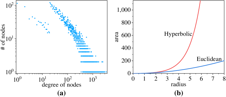
Figure 1. (a) The degree distribution of real-world network MovieLens. Coordinate axes are logarithmic. (b) Areas of circles on hyperbolic spaces (curvature $c=-1$) and Euclidean spaces, which shows that the hyperbolic spaces expand exponentially while Euclidean spaces expand polynomially.

Degree distributions of MovieLens and .

Hyperbolic spaces are those of constant negative curvatures, and are found to keep great representation capacity for data with hierarchical structures and power-law distributions due to the exponential expansion property (as shown in Figure 1(b)) (Krioukov et al., 2010; Peng et al., 2021). In the past few years, researchers have made some progress in representing hierarchical data in hyperbolic spaces (Nickel and Kiela, 2017; Liu et al., 2019; Chami et al., 2019; Zhang et al., 2021b; Wang et al., 2019; Nickel and Kiela, 2018; Sala et al., 2018; Yang et al., 2021). HTGN (Yang et al., 2021) attempts to embed dynamic graphs into hyperbolic geometry and achieves state-of-the-art performance. It adopts hyperbolic GCNs to capture spatial features and a hyperbolic temporal contextual attention module to extract the historical information. However, this method faces two major shortcomings. First, for some large graphs with long paths, the message propagation mechanism of GCNs is not effective enough because only direct neighbor nodes can be calculated in each step. Second, the temporal contextual attention module cannot handle the internal order of causal correlation in historical data and thus loses valid information for temporal evolutionary process.

To address the two aforementioned shortcomings of HTGN, in this paper, we propose a novel hyperbolic graph neural network model named HGWaveNet for temporal link prediction. In HGWaveNet, we first project the nodes into hyperbolic spaces. Then in the aspect of spatial topology, a hyperbolic diffusion graph convolution (HDGC) module is designed to learn node representations of each snapshot effectively from both direct neighbors and indirectly connected nodes. For temporal information, recurrent neural networks always emphasize short time memory while ignoring that of long time due to the time monotonic assumption (Cho et al., 2014), and the attention mechanism ignores the causal orders in temporality. Inspired by WaveNet (van den Oord et al., 2016) and Graph WaveNet (Wu et al., 2019a), we present hyperbolic dilated causal convolution (HDCC) modules to obtain hidden cumulative states of nodes by aggregating historical information and capturing temporal dependencies. In the training process of each snapshot, the hidden cumulative states and spatial-based node representations are fed into a hyperbolic gated recurrent unit (HGRU). The outputs of HGRU are regarded as the integration of spatial topological structures and temporal evolutionary information, and are utilized for final temporal link prediction. A hyperbolic temporal consistency (HTC) (Yang et al., 2021) component is also leveraged to ensure stability for tracking the evolution of graphs.

To conclude, the main contributions of this paper are as follows:

• We propose a novel hyperbolic graph neural network model named HGWaveNet for temporal link prediction, which learns both spatial hierarchical structures and temporal causal correlation of dynamic graphs.

• With regard to spatial topological structures, we design a hyperbolic diffusion graph convolution (HDGC) module to fit the power-law distributions of data and aggregate information from a wider range of nodes with greater effectiveness.

• For temporal evolution, we present hyperbolic dilated causal convolution (HDCC) modules to capture the internal causality between snapshots, and a hyperbolic temporal consistency (HTC) component is applied to remain stable when learning the evolution of graphs.

• We conduct extensive experiments on diverse real-world dynamic graphs. The results prove the superiority of HGWaveNet, as it has a relative improvement by up to 6.67% in terms of AUC over state-of-the-art methods.

2. Related Work

In this section, we systematically review the relevant works on temporal link prediction and hyperbolic graph representation learning.

2.1. Temporal Link Prediction

Temporal link prediction on dynamic graphs has attracted increasing interests in the past few years. Early methods usually use traditional algorithms or shallow neural architectures to represent structural and temporal information. For instance, CTDNE (Nguyen et al., 2018) captures the spatial and temporal information simultaneously by adding temporal constraints to random walk. Another example of using temporal random walk is DynNode2vec (Mahdavi et al., 2018), which updates the sampled sequences incrementally at each snapshot rather than generating them anew. DynamicTriad (Zhou et al., 2018) imposes the triad closure process and models the evolution of graphs by developing closed triads from open triads. Furthermore, Change2vec (Bian et al., 2019) improves this process and makes it applicable for dynamic heterogeneous graphs. HTNE (Zuo et al., 2018) integrates the Hawkes process into graph embedding to learn the influence of historical neighbors on current neighbors.

In contrast, graph neural network methods have recently received increasing attention. GCN (Welling and Kipf, 2016) provides an excellent node embedding pattern for general tasks on graphs, and most of later models take GCN or its variants, such as GraphSAGE (Hamilton et al., 2017) and GAT (Veličković et al., 2018), as basic modules for learning topological structures. GCRN (Seo et al., 2018) feeds node representations learned from GCNs into a modified LSTM to obtain the temporal information. Similar ideas are explored in EvolveGCN (Pareja et al., 2020), E-LSTM-D (Chen et al., 2019) and NTF (Wu et al., 2019b). The main difference between EvolveGCN and E-LSTM-D is that EvolveGCN could be considered as a combination of GCN and RNN while E-LSTM-D uses LSTM together with an encoder-decoder architecture. NTF takes a reverse order that characterizes the temporal interactions with LSTM before adopting the MLP for non-linearities between different latent factors, and sufficiently learns the evolving characteristics of graphs. To better blend the spatial and temporal node features, DySAT (Sankar et al., 2020) proposes applying multi-head self-attention. TGN (Rossi et al., 2020) leverages memory modules with GCN operators and significantly increases the computational efficiency. TNS (Wang et al., 2021) provides an adaptive receptive neighborhood for each node at any time. VRGNN (Hajiramezanali et al., 2019) models the uncertainty of node embeddings by regarding each node in each snapshot as a distribution.

However, the prevailing methods are built upon Euclidean spaces, which are not isometric with the power-law distributions of real-world graphs, and may cause distortion with the graph scale grows.

2.2. Hyperbolic Graph Representation Learning

Representation learning in hyperbolic spaces has been noticed due to their fitness to the hierarchical structures of real-world data. The significant performance advantages shown by the shallow Poincaré (Nickel and Kiela, 2017) and Lorentz (Nickel and Kiela, 2018) models spark more attempts to this issue. Integrated with graph neural networks, HGNN (Liu et al., 2019) and HGCN (Chami et al., 2019) are designed for graph classification and node embedding tasks separately. HAT (Zhang et al., 2021b) exploits attention mechanism for hyperbolic node information propagation and aggregation. LGCN (Zhang et al., 2021c) builds the graph operations of hyperbolic GCNs with Lorentzian version and rigorously guarantees that the learned node features follow the hyperbolic geometry. The above hyperbolic GNN-based models all adopt the bi-directional transition between a hyperbolic space and corresponding tangent spaces, while a tangent space is the first-order approximation of the original space and may inevitably cause distortion. To avoid distortion, H2H-GCN (Dai et al., 2021) develops a manifold-preserving graph convolution and directly works on hyperbolic manifolds. For practical application situations, HGCF (Sun et al., 2021a), HRCF (Yang et al., 2022c) and HICF (Yang et al., 2022a) study the hyperbolic collaborative filtering for user-item recommendation systems. Through hyperbolic graph learning, HyperStockGAT (Sawhney et al., 2021) captures the scale-free spatial and temporal dependencies in stock prices, and achieves state-of-the-art stock forecasting performance.

HVGNN (Sun et al., 2021b) and HTGN (Yang et al., 2021) fill the gap of hyperbolic models on dynamic graphs. HVGNN generates stochastic node representations of hyperbolic normal distributions via a hyperbolic graph variational autoencoder to represent the uncertainty of dynamics. HTGN adopts a conventional model architecture that handles the spatial and temporal information with HGCNs and contextual attention modules separately, however, ignores the causal order in the graph evolution. To further improve the hyperbolic graph models especially on temporal link prediction problem, we propose our HGWaveNet in terms of discrete dynamic graphs.

3. Preliminaries

In this section, we first give the formalized definitions of discrete dynamic graphs and temporal link prediction. Then some critical fundamentals about hyperbolic geometry are introduced.

3.1. Problem Definition

This paper discusses temporal link prediction on discrete dynamic graphs. Following  (Khoshraftar and An, 2022), we define discrete dynamic graphs as:

Definition 3.1 (Discrete Dynamic Graphs).

In discrete dynamic graph modeling, dynamic graphs can be viewed as a sequence of snapshots sampled from the original evolving process at consecutive time points. Formally, discrete dynamic graphs are represented as $\mathcal{G}=(\mathcal{G}_{0},\mathcal{G}_{1},\cdots,\mathcal{G}_{T})$, in which $\mathcal{G}_{t}$ is a snapshot at timestamp $t$. The time granularity for snapshot divisions could be hours, days, months or even years depending on specific datasets and applications.

Based on Definition 3.1, temporal link prediction is described as:

Definition 3.2 (Temporal Link Prediction).

The aim of temporal link prediction is to predict the links appeared in the snapshots after timestamp $t$ based on the observed snapshots before timestamp $t$. Formally, the model takes $(\mathcal{G}_{0},\mathcal{G}_{1},\cdots,\mathcal{G}_{t-1})$ as input in the training process, and then makes predictions on $(\mathcal{G}_{t},\mathcal{G}_{t+1},\cdots,\mathcal{G}_{T})$.

3.2. Hyperbolic Geometry of the Poincaré Ball

The $n$-dimensional hyperbolic space $(\mathbb{H}_{c}^{n},g^{c,\mathbb{H}})$ is the unique simply connected $n$-dimensional complete Riemannian manifold $\mathbb{H}_{c}^{n}$ with a constant negative curvature $-c(c>0)$, and $g^{c,\mathbb{H}}$ is the Riemannian metric. The tangent space $\mathcal{T}_{\textbf{x}}\mathbb{H}_{c}^{n}$ is a Euclidean, local, first-order approximation of $\mathbb{H}_{c}^{n}$ around the point $\textbf{x}\in\mathbb{H}_{c}^{n}$. Similar to  (Nickel and Kiela, 2017) and  (Ganea et al., 2018), we construct our method based on the Poincaré ball, one of the most widely used isometric models of hyperbolic spaces. Corresponding to $(\mathbb{H}_{c}^{n},g^{c,\mathbb{H}})$, the Poincaré ball $(\mathbb{B}_{c}^{n},g^{c,\mathbb{B}})$ is defined as

(1) $$\begin{split}&\mathbb{B}_{c}^{n}:=\left\{\textbf{x}\in\mathbb{R}^{n}:c\|\textbf{x}\|^{2}<1\right\},\\ &g^{c,\mathbb{B}}_{\textbf{x}}:=\left(\lambda_{\textbf{x}}^{c}\right)^{2}g^{E},\quad\lambda_{\textbf{x}}^{c}:=\frac{2}{1-c\|\textbf{x}\|^{2}},\end{split}$$

where $g^{E}=\textbf{I}_{n}$ is the Euclidean metric tensor.

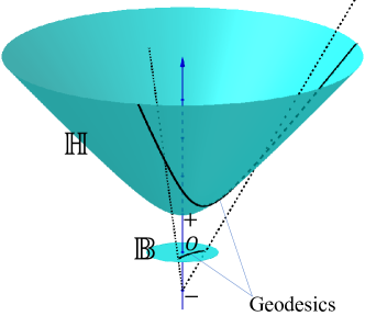
Figure 2. A hyperbolic manifold $\mathbb{H}$ and the corresponding Poincaré ball model $\mathbb{B}$. The distances on the manifolds are measured along geodesics.

The Poincaré ball model.

The Poincaré ball manifold $\mathbb{B}_{c}^{n}$ is an open ball of radius $1/\sqrt{c}$ (see Figure 2). The induced distance between two points $\textbf{x},\textbf{y}\in\mathbb{B}_{c}^{n}$ is measured along a geodesic and given by

(2) $$d_{c}\left(\textbf{x},\textbf{y}\right)=\frac{2}{\sqrt{c}}\cdot\tanh^{-1}\left(\sqrt{c}\|-\textbf{x}\oplus_{c}\textbf{y}\|\right),$$

in which the Möbius addition $\oplus_{c}$ in $\mathbb{B}_{c}^{n}$ is defined as

(3) $$\textbf{x}\oplus_{c}\textbf{y}:=\frac{\left(1+2c\langle\textbf{x},\textbf{y}\rangle+c\|\textbf{y}\|^{2}\right)\textbf{x}+\left(1-c\|\textbf{x}\|^{2}\right)\textbf{y}}{1+2c\langle\textbf{x},\textbf{y}\rangle+c^{2}\|\textbf{x}\|^{2}\|\textbf{y}\|^{2}}.$$

To map points between hyperbolic spaces and tangent spaces, exponential and logarithmic maps are given (Ganea et al., 2018). For $\textbf{x},\textbf{y}\in\mathbb{B}_{c}^{n},\textbf{v}\in\mathcal{T}_{\textbf{x}}\mathbb{B}_{c}^{n},\textbf{x}\neq\textbf{y}$ and $\textbf{v}\neq\textbf{0}$, the exponential map $\exp_{\textbf{x}}^{c}:\mathcal{T}_{\textbf{x}}\mathbb{B}_{c}^{n}\rightarrow\mathbb{B}_{c}^{n}$ is

(4) $$\exp_{\textbf{x}}^{c}(\textbf{v})=\textbf{x}\oplus_{c}\left(\tanh\left(\frac{\sqrt{c}\lambda_{\textbf{x}}^{c}\|\textbf{v}\|}{2}\right)\frac{\textbf{v}}{\sqrt{c}\|\textbf{v}\|}\right),$$

and the logarithmic map $\log_{\textbf{x}}^{c}:\mathbb{B}_{c}^{n}\rightarrow\mathcal{T}_{\textbf{x}}\mathbb{B}_{c}^{n}$ is

(5) $$\log_{\textbf{x}}^{c}(\textbf{y})=d_{c}\left(\textbf{x},\textbf{y}\right)\frac{-\textbf{x}\oplus_{c}\textbf{y}}{\lambda_{\textbf{x}}^{c}\|-\textbf{x}\oplus_{c}\textbf{y}\|},$$

where $\lambda_{\textbf{x}}^{c}$ and $d_{c}\left(\textbf{x},\textbf{y}\right)$ are the same as in Equations (1) and  (2). In our method, we use the origin point o as the reference point x to balance the errors in diverse directions.

4. Methodology

This section describes our proposed model HGWaveNet. First, we elaborate on the details of two core components: hyperbolic diffusion graph convolution (HDGC) and hyperbolic dilated causal convolution (HDCC). Then other key modules contributing to HGWaveNet are introduced, including gated HDCC, hyperbolic gated recurrent unit (HGRU), hyperbolic temporal consistency (HTC) and Fermi-Dirac decoder. Finally, we summarize the overall framework of HGWaveNet and analyse the time complexity.

4.1. Hyperbolic Diffusion Graph Convolution

Hyperbolic graph convolutional neural networks (HGCNs (Chami et al., 2019)) are built analogous to traditional GNNs. A typical HGCN layer consists of three key parts: hyperbolic feature transform

(6) $$\textbf{h}_{i}^{l,\mathbb{B}}=\textbf{W}^{l}\otimes_{c^{l-1}}\textbf{x}_{i}^{l-1,\mathbb{B}}\oplus_{c^{l-1}}\textbf{b}^{l},$$

attention-based neighbor aggregation

(7) $$\begin{split}\textbf{y}_{i}^{l,\mathbb{B}}&=\text{Agg}_{c^{l}}(\textbf{h}^{l,\mathbb{B}})_{i}\\ &=\exp_{\textbf{o}}^{c^{l}}\left(\text{Att}\left(\text{Concat}_{j\in\mathcal{N}(i)}\left(\log_{\textbf{o}}^{c^{l-1}}\left(\textbf{h}_{j}^{l,\mathbb{B}}\right)\right)\right)\right),\end{split}$$

and hyperbolic activation

(8) $$\textbf{x}_{i}^{l,\mathbb{B}}=\exp_{\textbf{o}}^{c^{l}}\left(\sigma\left(\log_{\textbf{o}}^{c^{l}}\left(\textbf{y}_{i}^{l,\mathbb{B}}\right)\right)\right),$$

in which $\textbf{W}^{l},\textbf{b}^{l}$ are trainable parameters and $\textbf{x}_{i}^{l,\mathbb{B}}$ is the representation of node $i$ at layer $l$ in manifold $\mathbb{B}_{c^{l}}^{n}$. Following (Yang et al., 2021), the matrix-vector multiplication $\otimes_{c}$ is defined as

(9) $$\textbf{M}\otimes_{c}\textbf{x}:=\exp_{\textbf{o}}^{c}\left(\textbf{M}\log_{\textbf{o}}^{c}\left(\textbf{x}\right)\right),\quad\textbf{M}\in\mathbb{R}^{n\times n},\textbf{x}\in\mathbb{B}_{c}^{n}.$$

However, the shallow HGCN can only aggregate information of direct neighbors and is not effective enough for large graphs with long paths. To overcome this shortcoming, we impose the diffusion process referring to  (Li et al., 2018). Consider a random walk process with restart probability $\alpha$ on $\mathcal{G}$, and a state transition matrix P (for most situations, P is the normalized adjacent matrix). Such Markov process converges to a stationary distribution $\mathcal{P}\in\mathbb{R}^{n\times n}$ after many steps, the $i$-th row of which is the likelihood of diffusion from node $i$. The stationary distribution $\mathcal{P}$ can be calculated in the closed form (Teng et al., 2016)

(10) $$\mathcal{P}=\sum_{k=0}^{\infty}\alpha(1-\alpha)^{k}\textbf{P}^{k},$$

where $k$ is the diffusion step. In practice, a finite $K$-step truncation of the diffusion process is adopted and separate trainable weight matrices are added to each step for specific objective tasks. Then, the diffusion convolution layer on graphs is defined as

(11) $$\textbf{Z}=\sum_{k=0}^{K}\textbf{A}^{k}\textbf{X}\textbf{W}_{k},$$

in which A is the bi-direct adjacent matrix, X is the input node features, $\textbf{W}_{k}$ is the weight matrix for the $k$-th diffusion step, and Z is the output node representations.

On account of the sparsity of real-world data, we convert the graph convolution into equivalent spatial domains for efficiency. Do all above operations in the hyperbolic space, and replace the summation in Equation (11) with an attention mechanism for better information aggregation. Then, the $k$-th step of hyperbolic diffusion graph convolution at layer $l$ is

(12) $$\textbf{X}_{k}^{l}=\text{HGCN}_{c_{k}^{l}}\left(\textbf{A}^{k},\textbf{X}^{l-1}\right),$$

where $\text{HGCN}_{c^{l}}(\cdot)$ is the conjunctive form of Equations (6),  (7), and  (8) with the adjacent matrix and node features as inputs. $\textbf{X}^{l}$ is calculated as

(13) $$\textbf{X}^{l}=\exp_{\textbf{o}}^{c^{l}}\left(\text{Att}\left(\text{Concat}_{k}\left(\log_{\textbf{o}}^{c_{k}^{l}}\left(\textbf{X}_{k}^{l}\right)\right)\right)\right).$$

Hyperbolic diffusion graph convolution is finally constructed with the stack of layers defined by Equations (13) and  (12), as sketched in Figure 3.

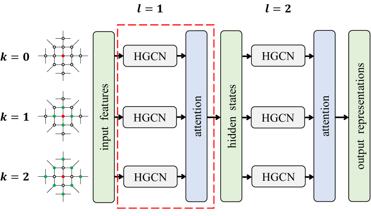
Figure 3. A hyperbolic diffusion graph convolution (HDGC) module with the number of layers $L=2$ and the number of diffusion steps $K=2$. The part in red dashed rectangle is a complete HDGC layer.

Hyperbolic diffusion graph convolution.

4.2. Hyperbolic Dilated Causal Convolution

Causal convolution refers to applying a convolution filter only to data at past timestamps (van den Oord et al., 2016), and guarantees that the order of data modeling is not violated, which means that the prediction $p(x_{t}|x_{0},x_{1},\cdots,x_{t-1})$ emitted by the model at timestamp $t$ cannot depend on future data $x_{t},x_{t+1},\cdots,x_{T}$. For 1-D temporal information, this operation can be implemented by shifting the output of a normal convolution with kernel size $S$ by $\lfloor S/2\rfloor$ steps, but a sufficiently large receptive field requires stacking many layers. To decrease the computational cost, dilated convolutions are adopted. By skipping the inputs with a certain step $d$, a dilated convolution applies its kernel over a larger area than its length, and with the stack of dilated convolution layers, the receptive field expands exponentially while preserving high computational efficiency. Based on the above definitions of causal convolutions and dilated convolutions, the dilated causal convolution operation in manifold $\mathbb{B}_{c}^{n}$ can be formalized mathematically as

(14) $$(\textbf{Z}_{i}\odot\textbf{F})_{t}=\exp_{\textbf{o}}^{c}\left(\sum_{s=0}^{S-1}\textbf{F}_{s}\log_{\textbf{o}}^{c}\left(\textbf{Z}_{i,t-d\times s}\right)\right),$$

where $d$ is the dilation step, $\textbf{Z}_{i,t}\in\mathbb{B}_{c}^{n}\ (t\leq T)$ is the representation of node $i$ at snapshot $\mathcal{G}_{t}$ and $\textbf{F}\in\mathbb{R}^{S\times n}$ denotes the kernels for all dimensions (also called channels). A stacked hyperbolic dilated causal convolution module is shown in Figure 4.

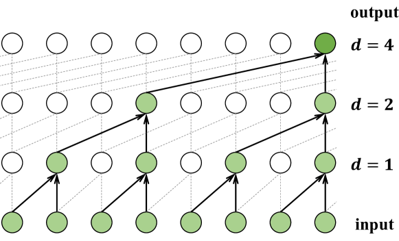
Figure 4. A stacked hyperbolic dilated causal convolution (HDCC) module with dilated depth $D=3$ and kernel size $S=2$. Each circle refers to one node at a timestamp. Under the exponentially large receptive field, each node preserves the temporal causal correlations with the past $S^{D}$ snapshots.

Hyperbolic dilated casual convolution.

Compared to attention-based historical information aggregation (Yang et al., 2021), HDCC can learn the internal order of causal correlation in temporality. Meanwhile, compared to RNNs, HDCC allows parallel computation and alleviates vanishing or exploding gradient problems due to its non-recursion(Wu et al., 2019a). Considering the superiority of HDCC on sequence problems, we leverage this module in handling the temporal evolutionary information of graphs.

4.3. Other Key Modules in HGWaveNet

Except for HDGC and HDCC, some other modules contribute greatly to our proposed HGWaveNet. Based on HDCC, we further design gated HDCC to preserve the valid historical information. Hyperbolic gated recurrent unit (HGRU) (Yang et al., 2021) is able to efficiently learn the latest node representations in Poincaré ball from historical states and current spatial characteristics. Additionally, as defined in  (Yang et al., 2021), hyperbolic temporal consistency (HTC) module provides a similarity constraint in temporality to ensure stability during graph evolution. Finally, a Fermi-Dirac decoder (Krioukov et al., 2010) is used to compute the probability scores for edge reconstruction.

4.3.1. Gated HDCC

As shown in the left part of Figure  5, we adopt a simple gating mechanism on the outputs of HDCCs. What is noteworthy is the use of logarithmic map before the Euclidean activation functions and exponential map after gating. The formulation is described as

(15) $$\textbf{H}_{i,t}=\exp_{\textbf{o}}^{c}\left(\tanh\left(\log_{\textbf{o}}^{c}\left(\left(\textbf{Z}_{i}\odot\textbf{F}_{1}\right)_{t}\right)\right)\cdot\sigma\left(\log_{\textbf{o}}^{c}\left(\left(\textbf{Z}_{i}\odot\textbf{F}_{2}\right)_{t}\right)\right)\right),$$

where $\textbf{F}_{1}$ and $\textbf{F}_{2}$ are different convolution kernels for two HDCCs, $\textbf{H}_{i,t}\in\mathbb{B}_{c}^{n}\ (t\leq T)$ is the historical hidden state of node $i$ at snapshot $\mathcal{G}_{t}$, and $\cdot$ denotes element-wise product. In addition, to enable a deeper model for learning more implicit information, residual and skip connections are applied throughout the gated HDCC layers.

4.3.2. Hyperbolic Gated Recurrent Unit

HGRU (Yang et al., 2021) is the hyperbolic variant of GRU (Cho et al., 2014). Performed in the tangent space, HGRU computes the output with high efficiency from historical hidden states and current input features, as

(16) $$\textbf{Z}_{i,t}=\exp_{\textbf{o}}^{c}\left(\text{GRU}\left(\log_{\textbf{o}}^{c}\left(\textbf{X}_{i,t}\right),\log_{\textbf{o}}^{c}\left(\textbf{H}_{i,t-1}\right)\right)\right).$$

In HGWaveNet, the historical hidden states are from gated HDCC module, so we use a single HGRU cell for just one step rather than linking it into recursion.

4.3.3. Hyperbolic Temporal Consistency

In real-world graphs, the evolution proceeds continuously. Correspondingly, the node representations are expected to change gradually in terms of temporality, which means that the node representations at two consecutive snapshots should keep a short distance. Hence, HTC (Yang et al., 2021) defines a similarity constraint penalty between $\textbf{Z}_{t-1}$ and $\textbf{Z}_{t}$ at snapshot $\mathcal{G}_{t}$ as

(17) $$\mathcal{L}_{\text{HTC}}^{t}=\frac{1}{N}\sum_{i=1}^{N}d_{c}\left(\textbf{Z}_{i,t-1},\textbf{Z}_{i,t}\right),$$

where $d_{c}(\cdot)$ is defined in Equation (2) and $N$ is the number of nodes. By adding the penalty in optimization process, HTC ensures that the node representations do not change rapidly and the stability of graph evolution is achieved.

4.3.4. Fermi-Dirac Decoder

As a generalization of sigmoid, Fermi-Dirac decoder (Krioukov et al., 2010) gives a probability score for edges between nodes $i$ and $j$, which fits the temporal link prediction problem greatly. It is defined as

(18) $$p_{{}_{F-D}}(\textbf{x}_{i},\textbf{x}_{j})=\frac{1}{\exp\left(\left(d_{c}\left(\textbf{x}_{i},\textbf{x}_{j}\right)-r\right)/s\right)+1},$$

where $r$ and $s$ are hyper-parameters, and $\textbf{x}_{i},\textbf{x}_{j}\in\mathbb{B}_{c}^{n}$ are hyperbolic representations of nodes $i$ and $j$.

4.4. Framework of HGWaveNet

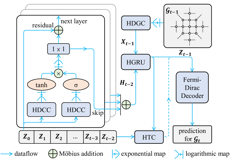
Figure 5. The overall framework of HGWaveNet. For $\mathcal{G}_{t-1}$, the historical evolutionary information handled by gated HDCCs and the spatial topological information handled by HDGC are fed into an HGRU module. With the constraint of HTC, the hyperbolic outputs are decoded by a Fermi-Dirac decoder and the temporal link prediction for $\mathcal{G}_{t}$ is made.

HGWaveNet.

With all modules introduced above, we now summarize the overall framework of HGWaveNet in Figure 5. For the snapshot $\mathcal{G}_{t-1}\in\mathcal{G}$, we first project the input node features into the hyperbolic space with exponential map, and then an HDGC module is applied to learn the spatial topological structure characteristics denoted by $\textbf{X}_{t-1}$. Simultaneously, the stacked gated HDCC layers calculate the latest historical hidden state $\textbf{H}_{t-2}$ from previous node representations $\textbf{Z}_{t-2},\textbf{Z}_{t-3},\cdots$ (the initial historical node representations are padded randomly at the beginning of training). Next, the spatial information $\textbf{X}_{t-1}$ and the temporal information $\textbf{H}_{t-2}$ are inputted into a single HGRU cell. The output of HGRU $\textbf{Z}_{t-1}$ is exactly the new latest node representations at snapshot $\mathcal{G}_{t-1}$, and is fed into the Fermi-Dirac decoder to make temporal link predictions for snapshot $\mathcal{G}_{t}$.

To maximize the probability of connected nodes in $\mathcal{G}_{t}$ and minimize the probability of unconnected nodes, we use a cross-entropy like loss $\mathcal{L}_{CE}^{t}$ defined as

(19) $$\begin{split}\mathcal{L}_{CE}^{t}=&\text{Avg}_{i\sim_{t}j}\left(-\log\left(p_{{}_{F-D}}\left(\textbf{Z}_{i,t-1},\textbf{Z}_{j,t-1}\right)\right)\right)+\\ &\text{Avg}_{i^{\prime}\nsim_{t}j^{\prime}}\left(-\log\left(1-p_{{}_{F-D}}\left(\textbf{Z}_{i^{\prime},t-1},\textbf{Z}_{j^{\prime},t-1}\right)\right)\right),\end{split}$$

in which $\sim_{t}$ denotes the connection at snapshot $\mathcal{G}_{t}$ between two nodes, and $\nsim_{t}$ is the opposite. $(i^{\prime},j^{\prime})$ is the sampled negative edge for accelerating training and preventing over-smoothing. Taking the HTC module into account and summing up all snapshots, the complete loss function is

(20) $$\mathcal{L}=\sum_{t=0}^{T}\left(\mathcal{L}_{CE}^{t}+\lambda\mathcal{L}_{HTC}^{t}\right).$$

Time Complexity Analysis

We analyse the time complexity of our proposed HGWaveNet by module for each snapshot. For the HDGC module, the computation is of $\mathcal{O}((Nd^{2}+|\mathcal{E}_{t}|Kd)L)$, where $d$ is the dimension of node representations, $|\mathcal{E}_{t}|$ is the edge number for snapshot $\mathcal{G}_{t}$, $K$ is the truncated diffusion steps and $L$ is the layer number of HDGC. For gated HDCC, the time complexity is $\mathcal{O}(S^{D}dD^{\prime})$, in which $S$ and $D$ are the kernel size and dilated depth of a single HDCC, respectively, and $D^{\prime}$ is the layer number of the complete gated HDCC module. HGRU and HTC run only once for each snapshot, and both take the time complexity of $\mathcal{O}(Nd)$. For Fermi-Dirac decoder, the time complexity is $\mathcal{O}(|\mathcal{E}_{t}|d+\tilde{|\mathcal{E}_{t}|}d)$, in which $\tilde{|\mathcal{E}_{t}|}$ is the number of negative samples for snapshot $\mathcal{G}_{t}$.

5. Experiments and Analysis

In this section, we conduct extensive experiments on six real-world graphs and prove the superiority of our proposed HGWaveNet. In addition, we also conduct ablation studies and hyper-parameter analysis to corroborate the three primary ideas of our method: the fitness between graph distributions and hyperbolic geometry, the effectiveness of spatial information from a wider range of neighbors aggregated by HDGC, and the causality of historical information in the evolutionary process learned by HDCC.

5.1. Experimental Setup

Table 1. Statistics of datasets.

Datasets	Enron	DBLP	AS733	FB	HepPh	MovieLens
# Nodes	184	315	6,628	45,435	15,330	9,746
# Edges	790	943	13,512	180,011	976,097	997,837
# Snapshots	11	10	30	36	36	11
Train : Test	8:3	7:3	20:10	33:3	30:6	8:3
$\delta$	1.5	2.0	1.5	2.0	1.0	2.0

5.1.1. Datasets

We evaluate our proposed model and baselines on six real-world datasets from diverse areas, including email communication networks Enron (Benson et al., 2018), academic co-author networks DBLP (Hajiramezanali et al., 2019) and HepPh (Leskovec et al., 2005), Internet router networks AS733 (Leskovec et al., 2005), social networks FB (Rossi and Ahmed, 2015) and movie networks MovieLens (Harper and Konstan, 2015). The statistics of these datasets are shown in Table 1. We take the same splitting ratios for training and testing as  (Yang et al., 2021) on all datasets except MovieLens on which a similar manner is adopted. Gromov’s hyperbolicity (GROMOV, 1987) $\delta$ is used to measure the tree-likeness and hierarchical properties of graphs. A lower $\delta$ denotes a more tree-like structure and $\delta=0$ denotes a pure tree. The datasets we choose all remain implicitly hierarchical and show distinct power-law distributions.

Table 2. Baselines.

Methods	Static/dynamic	Manifolds
HGCN (Chami et al., 2019)	Static	Lorentz
HAT(Zhang et al., 2021b)	Static	Poincaré
EvolveGCN (Pareja et al., 2020)	Dynamic	Euclidean
GRUGCN (Seo et al., 2018)	Dynamic	Euclidean
TGN (Rossi et al., 2020)	Dynamic	Euclidean
DySAT (Sankar et al., 2020)	Dynamic	Euclidean
HTGN (Yang et al., 2021)	Dynamic	Poincaré

5.1.2. Baselines

Considering that HGWaveNet is constructed in the hyperbolic space for dynamic graphs, we choose seven competing baselines either in hyperbolic spaces or built for dynamic graphs to verify the superiority of our model. The baselines are summarized in Table 2, where HTGN on Poincaré ball shows state-of-the-art performance in most evaluations.

Table 3. Performance on temporal link prediction.

	Dataset	Enron		DBLP		AS733		FB		HepPh		MovieLens
	Metric	AUC	AP	AUC	AP	AUC	AP	AUC	AP	AUC	AP	AUC	AP
Baselines	HGCN	$93.96\pm 0.09$	$93.55\pm 0.06$	$89.16\pm 0.16$	$91.63\pm 0.22$	$96.34\pm 0.05$	$93.28\pm 0.11$	$86.11\pm 0.13$	$83.74\pm 0.15$	$90.64\pm 0.07$	$88.98\pm 0.09$	$84.89\pm 0.40$	$77.98\pm 0.66$
	HAT	$94.49\pm 0.11$	$94.63\pm 0.08$	$89.29\pm 0.18$	$90.15\pm 0.14$	$96.09\pm 0.01$	$93.21\pm 0.02$	$84.02\pm 0.09$	$83.03\pm 0.15$	$90.52\pm 0.04$	$89.53\pm 0.04$	$86.26\pm 0.14$	$84.19\pm 0.21$
	EvolveGCN	$90.12\pm 0.69$	$92.71\pm 0.34$	$83.88\pm 0.53$	$87.53\pm 0.22$	$92.47\pm 0.04$	$95.28\pm 0.01$	$76.85\pm 0.85$	$80.87\pm 0.64$	$76.82\pm 1.46$	$81.18\pm 0.89$	$55.41\pm 1.55$	$69.41\pm 1.00$
	GRUGCN	$92.47\pm 0.36$	$93.38\pm 0.24$	$84.60\pm 0.92$	$87.87\pm 0.58$	$94.96\pm 0.35$	$96.64\pm 0.22$	$79.38\pm 1.02$	$82.77\pm 0.75$	$82.86\pm 0.53$	$85.87\pm 0.23$	$71.01\pm 0.77$	$79.04\pm 0.53$
	TGN	$91.77\pm 1.04$	$85.36\pm 0.87$	$87.20\pm 0.82$	$84.87\pm 0.80$	$93.19\pm 1.03$	$92.27\pm 0.83$	$80.85\pm 0.23$	$81.92\pm 1.34$	$74.78\pm 0.47$	$74.61\pm 0.43$	$71.52\pm 0.59$	$70.53\pm 0.38$
	DySAT	$93.06\pm 0.97$	$93.06\pm 1.05$	$87.25\pm 1.70$	$90.40\pm 1.47$	$95.06\pm 0.21$	$96.72\pm 0.12$	$76.88\pm 0.08$	$80.39\pm 0.14$	$81.02\pm 0.25$	$84.47\pm 0.23$	$70.21\pm 0.58$	$78.41\pm 0.33$
	HTGN	$94.17\pm 0.17$	$94.31\pm 0.26$	$89.26\pm 0.17$	$91.91\pm 0.07$	$98.75\pm 0.03$	$98.41\pm 0.03$	$83.70\pm 0.33$	$83.80\pm 0.43$	$91.13\pm 0.14$	$89.52\pm 0.28$	$86.80\pm 0.34$	$85.40\pm 0.19$
Ours	HGWaveNet	$96.86\pm 0.08$	$97.04\pm 0.07$	$89.96\pm 0.27$	$92.12\pm 0.18$	$98.78\pm 0.01$	$98.53\pm 0.02$	$89.51\pm 0.28$	$86.88\pm 0.29$	$92.37\pm 0.04$	$91.48\pm 0.05$	$91.90\pm 0.06$	$90.65\pm 0.12$
	Gain(%)	+2.51	+2.55	+0.75	+0.23	+0.03	+0.12	+3.95	+3.68	+1.36	+2.18	+5.88	+6.15
Ablation	w/o HDGC	$94.95\pm 0.10$	$95.24\pm 0.07$	$89.51\pm 0.24$	$91.84\pm 0.17$	$97.97\pm 0.20$	$97.35\pm 0.24$	$85.99\pm 0.29$	$82.77\pm 0.48$	$90.61\pm 0.22$	$89.68\pm 0.03$	$84.35\pm 0.12$	$82.77\pm 0.38$
	Gain(%)	-1.97	-1.85	-0.50	-0.30	-0.82	-1.20	-3.93	-4.73	-1.91	-1.97	-8.22	-8.69
	w/o HDCC	$95.33\pm 0.09$	$95.64\pm 0.09$	$89.56\pm 0.22$	$92.04\pm 0.12$	$97.83\pm 0.17$	$97.25\pm 0.21$	$85.13\pm 0.16$	$82.38\pm 0.88$	$90.83\pm 0.20$	$89.77\pm 0.32$	$82.46\pm 0.37$	$80.29\pm 0.58$
	Gain(%)	-1.58	-1.44	-0.44	-0.09	-0.96	-1.30	-4.89	-5.18	-1.67	-1.87	-10.27	-11.43
	w/o $\mathbb{B}$	$92.62\pm 0.55$	$93.77\pm 0.33$	$85.18\pm 0.29$	$87.76\pm 0.11$	$95.21\pm 0.11$	$96.85\pm 0.08$	$79.20\pm 0.34$	$82.45\pm 0.21$	$76.31\pm 0.75$	$78.11\pm 0.29$	$73.70\pm 0.54$	$80.15\pm 0.54$
	Gain(%)	-4.38	-3.37	-5.31	-4.73	-3.61	-1.71	-11.52	-5.10	-17.39	-14.62	-19.80	-11.58

Table 4. Performance on temporal new link prediction.

	Dataset	Enron		DBLP		AS733		FB		HepPh		MovieLens
	Metric	AUC	AP	AUC	AP	AUC	AP	AUC	AP	AUC	AP	AUC	AP
Baselines	HGCN	$90.36\pm 0.16$	$88.33\pm 0.55$	$81.20\pm 0.19$	$83.28\pm 0.23$	$92.33\pm 0.12$	$88.31\pm 0.16$	$81.04\pm 0.14$	$80.59\pm 0.13$	$89.64\pm 0.27$	$87.87\pm 0.11$	$85.27\pm 0.35$	$78.56\pm 0.49$
	HAT	$90.34\pm 0.10$	$88.60\pm 0.19$	$79.29\pm 0.15$	$82.58\pm 0.08$	$91.65\pm 0.08$	$90.13\pm 0.15$	$83.05\pm 0.10$	$82.96\pm 0.18$	$89.63\pm 0.05$	$88.34\pm 0.04$	$86.54\pm 0.16$	$84.60\pm 0.25$
	EvolveGCN	$82.85\pm 0.97$	$85.01\pm 0.22$	$73.49\pm 0.86$	$77.11\pm 0.44$	$75.82\pm 0.67$	$83.57\pm 0.46$	$74.49\pm 0.89$	$78.33\pm 0.66$	$74.79\pm 1.61$	$79.04\pm 1.02$	$55.45\pm 1.53$	$69.35\pm 0.98$
	GRUGCN	$87.59\pm 0.57$	$88.41\pm 0.45$	$75.60\pm 1.60$	$78.55\pm 1.05$	$83.14\pm 1.21$	$88.14\pm 0.76$	$77.69\pm 1.03$	$81.07\pm 0.77$	$81.97\pm 0.49$	$84.78\pm 0.22$	$71.32\pm 0.77$	$79.51\pm 0.50$
	TGN	$86.75\pm 0.59$	$81.37\pm 0.42$	$81.83\pm 1.08$	$81.61\pm 0.62$	$87.89\pm 0.63$	$84.94\pm 0.94$	$78.93\pm 0.98$	$76.57\pm 0.63$	$74.21\pm 0.78$	$76.12\pm 0.54$	$72.22\pm 0.68$	$70.90\pm 0.40$
	DySAT	$87.94\pm 3.78$	$86.83\pm 5.01$	$79.74\pm 4.35$	$83.47\pm 3.01$	$82.84\pm 0.72$	$89.07\pm 0.57$	$74.97\pm 0.12$	$78.34\pm 0.07$	$79.01\pm 0.26$	$82.53\pm 0.25$	$70.63\pm 0.58$	$79.02\pm 0.33$
	HTGN	$91.26\pm 0.27$	$90.62\pm 0.34$	$81.74\pm 0.56$	$84.06\pm 0.41$	$96.62\pm 0.22$	$95.52\pm 0.25$	$82.21\pm 0.41$	$81.70\pm 0.46$	$90.11\pm 0.14$	$88.18\pm 0.31$	$87.06\pm 0.25$	$85.82\pm 0.29$
Ours	HGWaveNet	$93.49\pm 0.08$	$92.51\pm 0.10$	$84.26\pm 0.46$	$86.19\pm 0.33$	$96.99\pm 0.07$	$95.60\pm 0.10$	$88.59\pm 0.28$	$86.00\pm 0.30$	$91.45\pm 0.05$	$90.21\pm 0.04$	$92.04\pm 0.04$	$90.66\pm 0.07$
	Gain(%)	+2.44	+2.09	+2.97	+2.53	+0.38	+0.08	+6.67	+3.66	+1.49	+2.12	+5.72	+5.64
Ablation	w/o HDGC	$90.67\pm 0.20$	$89.90\pm 0.22$	$83.47\pm 0.36$	$85.85\pm 0.28$	$95.69\pm 0.34$	$93.99\pm 0.36$	$84.96\pm 0.30$	$81.57\pm 0.42$	$89.63\pm 0.26$	$88.27\pm 0.03$	$84.76\pm 0.15$	$83.42\pm 0.33$
	Gain(%)	-3.02	-2.82	-0.94	-0.39	-1.34	-1.68	-4.10	-5.15	-1.99	-2.15	-7.91	-7.99
	w/o HDCC	$91.76\pm 0.08$	$90.87\pm 0.06$	$82.36\pm 0.23$	$84.87\pm 0.10$	$94.56\pm 0.44$	$92.91\pm 0.45$	$84.03\pm 0.14$	$80.99\pm 0.76$	$89.87\pm 0.20$	$88.42\pm 0.30$	$82.92\pm 0.31$	$81.23\pm 0.50$
	Gain(%)	-1.85	-1.77	-2.25	-1.53	-2.51	-2.81	-5.15	-5.83	-1.73	-1.98	-9.91	-10.40
	w/o $\mathbb{B}$	$87.10\pm 0.72$	$88.49\pm 0.57$	$76.65\pm 0.80$	$79.53\pm 0.67$	$84.85\pm 0.77$	$89.59\pm 0.37$	$77.37\pm 0.33$	$80.63\pm 0.19$	$74.23\pm 0.58$	$76.21\pm 0.53$	$74.11\pm 0.55$	$80.51\pm 0.31$
	Gain(%)	-6.83	-4.35	-9.03	-7.73	-12.52	-6.29	-12.67	-6.24	-18.83	-15.52	-19.48	-11.20

5.1.3. Evaluation Tasks and Metrics

Similar to  (Yang et al., 2021), our experiments consist of two different tasks: temporal link prediction and temporal new link prediction. Specifically, temporal link prediction aims to predict the edges that appear in $\mathcal{G}_{t}$ and other snapshots after timestamp $t$ based on the training on $(\mathcal{G}_{0},\mathcal{G}_{1},\cdots,\mathcal{G}_{t-1})$, while temporal new link prediction aims to predict those in $\mathcal{G}_{t}$ but not in $\mathcal{G}_{t-1}$. To quantify the experimental performance, we choose the widely used metrics average precision (AP) and area under ROC curve (AUC). The datasets are split into training sets and test sets as shown in Table 1 by snapshots to run both our proposed model and baselines on the above tasks.

5.2. Experimental Results

We implement HGWaveNet with PyTorch on Ubuntu 18.04. Each experiment is repeated five times to avoid random errors, and the average results (with form average value $\pm$ standard deviation) on the test sets are reported in Table LABEL:tab::exper:link and Table 4. Next, we discuss the experimental results on each evaluation task separately.

5.2.1. Temporal Link Prediction

The results on temporal link prediction are shown in Table LABEL:tab::exper:link. Obviously, our HGWaveNet outperforms all baselines including the hyperbolic state-of-the-art model HTGN both on AUC and AP. To analyse the results further, we intuitively divide the six datasets into two groups: small (Enron, DBLP, AS733) and large (FB, HepPh, MovieLens), according to the scales. It can be observed that the superiority of our model is more significant on large graphs than small ones compared with baselines, especially those Euclidean methods. This is because the representation capacity of Euclidean methods decreases rapidly with increasing graph scales, while hyperbolic models remain stable by virtue of the fitness between data distributions and space properties.

5.2.2. Temporal New Link Prediction

The results on temporal new link prediction are shown in Table 4. This task aims to predict the edges unseen in the training process and evaluates the inductive ability of models. Our model shows greater advantages, and similar gaps with those on temporal link prediction between small and large graphs appear again. Another observed fact is that even for the inductive evaluation task, the two hyperbolic static methods HGCN and HAT have a relatively better performance than the Euclidean dynamic models. This observation further demonstrates the excellence of modeling real-world graphs on hyperbolic spaces.

5.3. Ablation Study

To asses the contribution of each component, we conduct the following ablation study on three HGWaveNet variants:

• w/o HDGC: HGWaveNet without the hyperbolic diffusion graph convolution, implemented by replacing HDGC with shallow HGCN to learn from spatial characteristics.

• w/o HDCC: HGWaveNet without the hyperbolic dilated causal convolution, implemented by replacing HDCC with an attention mechanism to achieve historical hidden states.

• w/o $\mathbb{B}$: HGWaveNet without hyperbolic geometry, implemented by replacing all modules with corresponding Euclidean versions.

We take the same experimental setup with HGWaveNet and baselines on these three variants, and the results are reported in the last rows of Table LABEL:tab::exper:link and Table 4. The performance drops noticeably after removing any of these three components, which indicates their respective importance. In the following, we discuss the details of the effectiveness of these variants.

HDGC module imposes the diffusion process into hyperbolic graph convolution networks. It allows nodes to aggregate information from a wider range of neighbors and improves the efficiency of message propagation by calculating the stationary distribution of a long Markov process in a closed form. The fact that performance of w/o HDGC variant has a larger degradation on large graphs than small ones forcefully proves the effectiveness of this component for large graphs with long paths.

The purpose of HDCC module is to capture the internal order of causal correlation in sequential data. Generally, the larger a graph is, the more complex its evolution is and the richer historical information it has. The experimental results on w/o HDCC show the powerful ability of this component to capture causal order in temporal evolution process, especially on complex graphs (i.e. FB and MovieLens).

As observed in Table LABEL:tab::exper:link and Table 4, the degradation of w/o $\mathbb{B}$ is much more severe than that of the other two variants, which strongly supports our primary idea that hyperbolic geometry fits the power-law distributions of real-world graphs very well. Moreover, it is noteworthy that for most results, the variant w/o $\mathbb{B}$ exhibits a comparable or even exceeding performance to other Euclidean baselines. This proves that our model architecture still keeps advanced even without the advantages of hyperbolic geometry.

5.4. Parameter Analysis

We further study the influences of three hyper-parameters: representation dimension, truncated diffusion step and dilated depth.

We evaluate the performance of HGWaveNet and one of the best Euclidean models GRUGCN on two datasets FB (relatively sparse) and MovieLens (relatively dense) by setting the representation dimension into different values, as shown in Figure 6. On the one hand, it is clear that with the dimension decreasing, our model remains stable compared to GRUGCN, to which the hyperbolic geometry contributes greatly. On the other hand, for HGWaveNet, the degradation of the performance on MovieLens is severer than that on FB, which is consistent with the conclusion in  (Zhang et al., 2021a) that hyperbolic models fit sparse data better than dense data.

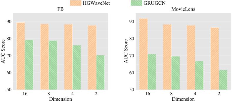
Figure 6. The influence of representation dimension on two datasets FB and MovieLens for HGWaveNet and GRUGCN.

Influence of dimension.

Figure 7 shows the results of our model for temporal link prediction on MovieLens with different values of truncated diffusion step $K$ in HDGC and dilated depth $D$ in HDCC. The wrap-up observation that the performance generally increases as $K$ and $D$ increase proves the positive influences of diffusion process and dilation convolution. Specifically, in terms of truncated diffusion step, the performance has a great improvement from $K=1$ to $K=2$. When $K>2$, the benefit from increasing $K$ becomes too small to match the surge of computation from exponentially expanding neighbors in graphs. Dilated depth $D$ is used to control the receptive field of causal convolution. However, as the receptive field expands, more noise is imported and may degrade the model performance. According to our extensive experiments, $D=3$ is a nice choice in most situations, with the causal convolution kernel size being 2.

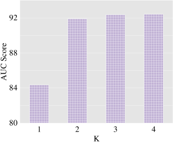
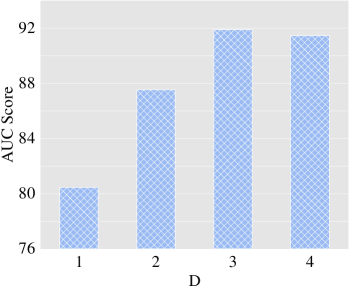
Figure 7. The influence of truncated diffusion step $K$ (left) and dilated depth $D$ (right) on MovieLens.

Influence of truncated diffusion step and dilated depth.

6. Conclusion

In this paper, we propose a hyperbolic graph neural network HGWaveNet for temporal link prediction. Inspired by the observed power-law distribution and implicit hierarchical structure of real-world graphs, we construct our model on the Poincaré ball, one of the isometric models of hyperbolic spaces. Specifically, we design two novel modules hyperbolic diffusion graph convolution (HDGC) and hyperbolic dilated causal convolution (HDCC) to extract the spatial topological information and temporal evolutionary states, respectively. HDGC imposes the diffusion process into graph convolution and provides an efficient way to aggregate information from a wider range of neighbors. HDCC ensures that the internal order of causal correlations is not violated by applying the convolution filter only to previous data. Extensive experiments on diverse real-world datasets prove the superiority of HGWaveNet, and the ablation study further verifies the effectiveness of each component of our model. In future work, we will further generalize our model for more downstream tasks and try to use hyperbolic GNNs to capture more complex semantic information in heterogeneous graphs.

Appendix A Appendix

A.1. Notations

Part of notations in our paper are summarized in Table 5.

Table 5. Notations.

Symbols	Descriptions
$\mathcal{G}$	Discrete dynamic graph represented by snapshots.
$\mathcal{G}_{t}$	Snapshot of $\mathcal{G}$ at timestamp $t$.
$\mathbb{H}_{c}^{n}$	$n$-dimensional hyperbolic manifold with curvature $-c$.
$g^{c,\mathbb{H}}$	Riemannian metric corresponding to the manifold $\mathbb{H}$.
$\mathcal{T}_{\mathbf{x}}\mathbb{H}_{c}^{n}$	Tangent space of $\mathbb{H}_{c}^{n}$ at point $\mathbf{x}$.
$\mathbb{B}_{c}^{n}$	Poincaré ball manifold corresponding to $\mathbb{H}_{c}^{n}$.
$d$	Dimension of node representations.
$K$	Truncated diffusion steps in HDGC.
$L$	Layer number of HDGC.
$S$	Convolution kernel size of HDCC.
$D$	Dilated depth of HDCC.
$D^{\prime}$	Layer number of gated HDCC module.
$\mathbf{A}$	Bi-direct adjacent matrix of a static graph or snapshot.
$\mathbf{X}_{t,k}^{l}$	$k$-th step of HDGC at layer $l$, timestamp $t$.
$\mathbf{H}_{t}$	Temporal information earlier than timestamp $t$.
$\mathbf{F}$	Kernel metrix of HDCC.
$\mathbf{Z}_{t}$	Node representations at timestamp $t$.
$\mathcal{L}_{\text{HTC}}^{t}$	Hyperbolic temporal consistency at timestamp $t$.
$\mathcal{L}_{\text{CE}}^{t}$	Cross-entropy like loss at timestamp $t$.
$\mathbf{W},\mathbf{b}$	Trainable parameters.

A.2. Experimental Details

For all baselines, we take the recommended parameter settings unless otherwise noted. For our proposed HGWaveNet, the parameters are set as follows: the truncated diffusion step $K=2$, the layer number of HDGC $L=2$, the dilation depth for HDCC $D=3$, kernel size $S=2$, the layer number for gated HDCC is valued as 4, and the hyper-parameters $r,s$ in Fermi-Dirac decoder are taken to be 2 and 1 separately. All involved curvatures are initialized as 1 and keep trainable during the training process. For fairness, the representation dimension is set to 16 for all methods. All experiments are run on a machine with 2 $\times$ Intel Xeon Gold 6226R 16C 2.90 GHz CPUs, 4 $\times$ GeForce RTX 3090 GPUs.

A.3. Supplementary Experiments

In Table 6,  7 and  8, we give out the supplementary experimental results for parameter analysis in Section 5.4. All these experiments are evaluated by AUC score on temporal link prediction task.

Table 6. The influence of representation dimension.

Dimension	Enron	DBLP	AS733	FB	HepPh	MovieLens
16	96.86	89.96	98.78	89.51	92.37	91.90
8	96.56	89.49	98.67	88.74	90.20	88.44
4	96.64	89.24	98.36	88.51	88.76	87.90
2	96.41	88.84	97.95	87.87	88.42	86.55

Table 7. The influence of truncated diffusion step $K$.

$K$	Enron	DBLP	AS733	FB	HepPh	MovieLens
1	94.95	89.51	97.97	85.99	90.61	84.35
2	96.86	89.96	98.78	89.51	92.37	91.90
3	96.88	89.62	98.95	90.28	92.72	92.36
4	96.86	89.67	98.94	90.39	92.81	92.42

Table 8. The influence of dilated depth $D$.

$D$	Enron	DBLP	AS733	FB	HepPh	MovieLens
1	91.14	88.67	94.98	73.69	87.38	80.44
2	92.16	89.89	97.12	83.18	90.41	87.52
3	96.86	89.96	98.78	89.51	92.37	91.90
4	97.17	89.62	98.93	89.99	93.17	91.47