Road Network Representation Learning: A Dual Graph based Approach
Abstract.
Road network is a critical infrastructure powering many applications including transportation, mobility and logistics in real life. To leverage the input of a road network across these different applications, it is necessary to learn the representations of the roads in the form of vectors, which is named road network representation learning (RNRL). While several models have been proposed for RNRL, they capture the pairwise relationships/connections among roads only (i.e., as a simple graph), and fail to capture among roads the high-order relationships (e.g., those roads that jointly form a local region usually have similar features such as speed limit) and long-range relationships (e.g., some roads that are far apart may have similar semantics such as being roads in residential areas). Motivated by this, we propose to construct a hypergraph, where each hyperedge corresponds to a set of multiple roads forming a region. The constructed hypergraph would naturally capture the high-order relationships among roads with hyperedges. We then allow information propagation via both the edges in the simple graph and the hyperedges in the hypergraph in a graph neural network context. In addition, we introduce different pretext tasks based on both the simple graph (i.e., graph reconstruction) and the hypergraph (including hypergraph reconstruction and hyperedge classification) for optimizing the representations of roads. The graph reconstruction and hypergraph reconstruction tasks are conventional ones and can capture structural information. The hyperedge classification task can capture long-range relationships between pairs of roads that belong to hyperedges with the same label. We call the resulting model HyperRoad. We further extend HyperRoad to problem settings when additional inputs of road attributes and/or trajectories that are generated on the roads are available. We conduct extensive experiments on two real datasets, for five downstream tasks, and under four problem settings, which demonstrate that our model achieves impressive improvements compared with existing baselines across datasets, tasks, problem settings and performance metrics.
1. Introduction
Road network is a fundamental infrastructure supporting many real life applications, including but not limited to transportation, logistics, mobility, city management, planning, etc. Correspondingly, for various tasks such as traffic inference and forecasting (guo2019attention, 6), road tag prediction (yin2021multimodal, 41) and arrival time estimation (yuan2020effective, 42), the road network data is used as a key input. Nevertheless, road network in its raw form cannot be directly inputted to machine learning models designed for these tasks. A common practice is to learn representations of a road network (specifically its roads) in the forms of vectors, called road network representation learning (RNRL), which captures essential information of the road network, and then use the learned representations for various downstream tasks (wang2019learning, 33, 11, 36, 2).
What is intrinsic to a road network is its structural information, which refers to the roads of the road network and the connections among the roads. Quite a few models have been proposed to capture the structural information of a road network for RNRL (wang2019learning, 33, 11, 36, 2). Among them, some studies (wang2019learning, 33, 2) follow the node2vec idea and some others (jepsen2020relational, 11, 36) adopt graph neural networks (GNN). Specifically, in (wang2019learning, 33, 2), it first collects some paths, each corresponding to a sequence of roads, via shortest path sampling (wang2019learning, 33) or random walks (chen2021robust, 2), and then learns the representations of roads via the skip-gram model (mikolov2013distributed, 21) based on collected paths. In (jepsen2020relational, 11, 36), it feeds the graph structure that models the structural information of a road network to GNN and learns the representations of roads by optimizing a graph reconstruction pretext task. It can be observed that all these models model the structural information of a road network as a simple graph and captures only pairwise connections/relationships among roads for RNRL.
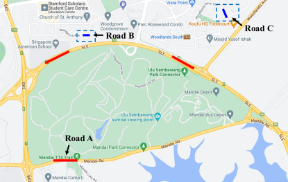
We observe that apart from pairwise relationships, high-order relationships and long-range relationships commonly exist in road networks, yet the latter two are hardly captured by the simple graph structure used by existing models (wang2019learning, 33, 11, 36, 2). Here, a high-order relationship is one among more than two roads and a long-range relationship is one among two roads that are not necessarily to have close spatial proximity. For an example of the high-order relationships, consider the three roads marked in red in Fig. 1. These roads together with some others surrounding a park region (the area in green in the middle of the figure) constitute a highway loop. This relationship involves many roads and thus it is a high-order relationship, which helps identify the urban function of “Road A”. However, existing models (wang2019learning, 33, 11, 36, 2) fail to capture this high-order relationship and may learn low-quality representations. For example, for “Road A” in the figure, existing GNN-based models may misinterpret its function and generate its representation mainly based on its pairwise connections with walk roads nearby. For an example of the long-range relationship, consider the two roads marked in blue in Fig. 1, namely “Road B” and “Road C”. These two roads share similar information (e.g., they are both residential roads with low speed limit), despite being far apart on the map. Again, existing models (wang2019learning, 33, 11, 36, 2) are largely incapable of capturing this long-range relationship.
In this paper, we propose a solution called HyperRoad (Hypergraph-Oriented Road network representation), which is capable of capturing the pairwise, high-order and long-range relationships among the roads all at the same time. We explain its intuitions and major ideas as follows. First, based on the observation that some roads that form a region may have some similarity in terms of semantics and functions (e.g., a highway loop), we propose to first extract all regions that are naturally formed by roads (details will be introduced in Section 3.1). Then for each extracted region, we construct a hyperedge connecting all the roads that form the region. The constructed hyperedges would naturally capture the high-order relationships among the roads and constitute a hypergraph. For example, for the road network shown in Fig. 1, we would extract a region that corresponds to the park and construct a hyperedge connecting all roads that constitute the highway loop surrounding the park.
Second, we design a dual-channel aggregating mechanism for propagating the information through two channels in a context of GNN, one for the simple graph and the other for the constructed hypergraph. We then fuse the aggregated information from two channels via a gating mechanism as the road embeddings. This dual-channel aggregating mechanism has its power reflected by (1) it captures the pairwise relationships via the channel based on simple graph as existing models do, and (2) it captures high-order relationships via the channel based on the hypergraph (which is new). It is worth noting that although hypergraph and hypergraph neural network have been applied to enhance spatial-temporal mining in some existing works (xia2021spatial, 37, 19), our work is the first attempt to leverage the power of hypergraph for the RNRL problem and more generally road network modeling.
Third, we design a bi-level self-supervised learning module for optimizing the road embeddings. At the simple graph level, we adopt the graph reconstruction pretext task as some existing models do (jepsen2020relational, 11, 36). At the hypergraph level, we adopt two pretext tasks, namely hypergraph reconstruction and hyperedge classification. The hypergraph reconstruction task is natural for hypergraph representation learning. The hyperedge classification task, which is to perform a classification task on hyperedges (with the labels defined based on some intrinsic properties of hyperedges such as their sizes), is newly proposed for the constructed hyperedges based on road networks. The hyperedge classification task can capture long-range relationships between pairs of roads that belong to hyperedges with the same label.
Apart from the structural information, some other types of information are associated with or closely related to a road network and have been used for RNRL. These include (1) spatial information, which refers to the locations of roads (e.g., the coordinates of the middle points of roads), (2) road attributes (e.g., road type, lane number, etc), and (3) trajectories, which are sequences of roads that are generated by vehicles on the roads. Different from the structural and spatial information, the attributes and trajectories are not always available for RNRL. For example, for the road networks we downloaded from OpenStreetMap in City Xi’an, the lane attribute is missing for 69% of the roads. The trajectories are available for some specific cities only and even for those cities some trajectories are available, they are not complete and cover only a small fraction of roads. Therefore, we tackle the RNRL problem under four settings depending on the availability of the attributes and trajectories. The default setting is that we only have the structural and spatial information since it is deemed to be intrinsic to a road network. Other settings include one with additional attributes, one with additional trajectories, and the last one with both additional attributes and trajectories. For the default setting, we incorporate a position-aware embedding generation module, which embeds the location of each road into its embedding to be inputted to the dual-channel aggregating mechanism. We still call the resulting model HyperRoad. For the setting with the additional attributes, we incorporate the attribute embeddings to the initial embeddings of roads and introduce an additional pretext task of attribute reconstruction in the bi-level self-supervised learning module. We call the resulting model HyperRoad-A. For the setting with the additional trajectories, we follow an existing study (chen2021robust, 2) and introduce a BERT like structure on top of HyperRoad for fine-tuning the road embeddings learnt by HyperRoad with the trajectories. We call the resulting model HyperRoad-T. For the setting with both additional attributes and additional trajectories, we merge HyperRoad-A and HyperRoad-T and obtain a model called HyperRoad-AT.
To summarize, our contributions are three-fold:
-
•
We observe the insufficiency of existing RNRL models for capturing the high-order relations and long-range relations among roads. We then design a novel model called HyperRoad, which (1) constructs a hypergraph on the road network for the first time based on how roads form regions, (2) involves a dual-channel aggregating mechanism based on both the simple graph of the road network and the constructed hypergraph for capturing the pairwise and high-order relationships at the same time, and (3) uses a bi-level self-supervised learning module, which involves quite a few pretext tasks at both the simple graph level and the hypergraph level, for optimizing the road embeddings as well as capturing long-range relationships. In this way, our model is capable of capturing the pairwise, high-order and long-range relationships among the roads all at the same time. (Section 3)
-
•
We summarize the types of information of a road network, which can be used for RNRL. They include structural and spatial information (which is intrinsic and always available) and road attributes and trajectories (which are not always available or complete). Correspondingly, we identify four settings for RNRL depending on the availability of the road attributes and trajectories and propose corresponding solutions all with HyperRoad as the core. This shows that our HyperRoad model is fundamental and can be enhanced flexibly when additional information is available. This is the first systematical study on various settings of RNRL. (Section 4)
-
•
We conduct extensive experiments on two real datasets for five downstream tasks including both road based and trajectory based ones under different problem settings. The results show that our model outperforms existing models across all tasks, under all settings, and on both datasets. (Section 5 and 6)
2. Problem Statement
We consider four types of information, which are associated with or closely related to a road network and have been used for road network representation learning (RNRL). These include (1) structural information, which refers to a set of roads (or nodes) and the pairwise connections among them, (2) spatial information, which refers to the locations of roads (e.g., the coordinates of the middle points of roads), (3) road attributes (e.g., road type, lane number, etc), and (4) trajectories, which are sequences of roads that are generated by vehicles on the roads. We introduce some notations of the four types of information as follows.
Structural information. It is usually represented by a simple (directed) graph , where is a set of nodes each representing a road and is a set of edges. The corresponding adjacency matrix of is represented as , where the entry is a binary value indicating whether there exists a link from road to road . The structural information is intrinsic to the road network.
Spatial information. Each node (or road) has a coordinate vector () including the latitude and longitude of its middle point, mapping the road into the geographic space. Spatial information is another type of intrinsic information of road network.
Road attributes. For a road , we denote its road attributes as , where denotes the number of attributes of . The road attributes convey some semantics information of roads.
Trajectories. A trajectory corresponds to a sequence of adjacent roads, where is a road in . The trajectories on a road network can reflect the mobility patterns on the road network.
Problem statement. Formally, the road network representation learning (RNRL) problem is to learn a low dimensional vector representation for each road, denoted as with as the embedding size. Among the four types of information, the structural and spatial information is intrinsic information and always available, while the attributes and trajectories are not always available or complete. Therefore, we study the RNRL problem under four settings depending on the availability of the attributes and trajectories. The default setting is that we only have the intrinsic structural and spatial information. Other settings include one with additional attributes, one with additional trajectories, and the last one with both additional attributes and trajectories.
3. HyperRoad: The Core
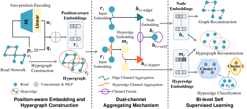
In this section, we propose a novel model called HyperRoad for road network representation learning (RNRL). The overview of the model architecture is shown in Fig. 2. HyperRoad is based on three key ideas: (1) it incorporates a positional encoding scheme for embedding the roads (called position-aware embedding) and constructs a hypergraph, where each hyperedge corresponds to a set of multiple roads forming a region, (2) it propagates information via both edges (of a simple graph capturing the pairwise relationships) and hyperedges (of the constructed hypergraph) in a context of graph neural network, and (3) it optimizes the road representations with a few pretext tasks based on both the simple graph (i.e., graph reconstruction) and the constructed hypergraph (including hypergraph reconstruction and hyperedge classification). Next, we introduce these three ideas in turn.
3.1. Position-aware Embedding and Hypergraph Construction
Position-aware Embedding. To represent the innate spatial information in road networks, we follow the strategy in BERT (devlin2018bert, 3) to jointly embed roads’ IDs and locations into dense representations as the model inputs. Specifically, for each road , we introduce an embedding layer to encode its ID as an embedding vector . Here, an embedding layer corresponds to a special MLP layer without bias and non-linear function. All road IDs’ embeddings are represented as an embedding matrix , which will be learned in an end-to-end manner.
In addition, inspired by the positional encoding of transformers (devlin2018bert, 3) and spatial representation learning (mai2020multi, 20), we propose a positional encoder module to encode the spatial information of a road network. In specific, given the coordinate vector of a road , we use sine and cosine functions of different frequencies to generate its positional encoding as follows.
| (1) |
where denotes the embedding size (which is a multiple of 4), is an integer in [0, d/4-1], and denote the projected latitude and longitude values, respectively, is the scale parameter to constrain the magnitude of projected values, and is the frequency parameter similar to the positional encoding in transformers. The difference from those conventional positional encoding in transformers, which consider 1D positions, is that we consider 2D locations in geospace.
Finally, for each road , we fuse its ID embedding and positional embedding into a single one as follows.
| (2) |
where is the concatenate operation and MLP is a fully connected neural network.
Hypergraph Construction. As explained in Section 1, there would usually exist some high-order relationships among roads that form a region. For example, those roads that constitute a highway loop surrounding a park in Fig. 1 would tend to have similar semantics (e.g., highway roads). Therefore, we propose to construct hyperedges based on how roads form regions. Specifically, we apply a map segmentation algorithm proposed in (yuan2012discovering, 43) to find the polygons that are formed by roads. Note this process is based on the structural and spatial information of a road network solely. Then, for each found polygon, we construct a hyperedge, which involves all roads that constitute the polygon. There are two major benefits with the constructed hypergraph. First, the constructed hyperedges would naturally capture the high-order relationships among roads of a road network. Second, as will be shown in the next section (Section 3.3), the intrinsic properties associated with the constructed hyperedges (e.g., its size) can be used as inductive bias to design new self supervised learning pretext tasks for learning the representations of roads with long-range relationships.
Formally, a hypergraph based on the road network is defined as , where is a set of roads, and represents the set of hyperedges. The topological structure of can also be represented by an incidence matrix , with entries defined as follows.
| (3) |
3.2. Dual-channel Aggregating Mechanism
An overview of the Dual-channel Aggregating Mechanism is shown in Fig. 2 (the middle part). In this module, it iteratively aggregates the information from related roads to encode the structures. The intuition is that the edge level neighborhoods in the simple graph capture pairwise relationships among roads and local receptive fields, and the hyperedge level neighborhoods in the hypergraph capture the complex high-order relationships. Both are indispensable and complementary for road modeling. For example, the hyperedge context (e.g., highway loop) and local environment (e.g., residential area) can jointly determine the function of a ramp road. Therefore, we conduct message aggregation via two channels, namely edge channel and hyperedge channel, and devise a novel dual-channel aggregating mechanism. Note that some existing GNN methods (morris2019weisfeiler, 22, 34) also model high-order node relationships to help expand the receptive fields and/or improve the expressiveness of GNN model. For example, -GNNs (morris2019weisfeiler, 22) aggregates the information from high-order neighbors defined by the -order cliques, and TDGNN (wang2021tree, 34) aggregates the information from multi-hop neighbors defined by the tree decomposed subgraphs. These methods define different structures on the same simple graph. In contrast, our aggregation mechanism takes a dual graph perspective and aggregates information from both simple graph and hypergraph. In fact, we are aware of no existing methods which use multiple channels to combine a simple graph and a hypergraph together as ours does. In this section, we first illustrate the design of one-layer aggregation and then generalize it to multiple layers.
Edge Channel Aggregation. The goal of this sub-module is to propagate node information from the simple graph contexts. This process can be formulated as follows.
| (4) |
where is the message received by node from the edge channel at layer , denotes hidden state of node at layer ( is set to be the position-aware input embedding for node ), denotes the neighborhoods of node defined by edges in , and is an aggregation function, which is implemented as a mean aggregator in this paper to keep the model simple.
| (5) |
where is a trainable weight matrix to distill useful information for propagation and the normalization term is to constrain the embedding scales.
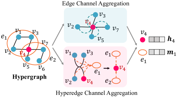
Hyperedge Channel Aggregation. The hyperedge channel aggregation is based on the following two-step operations.
| (6) | |||
where is the aggregated hyperedge representation of at layer , denotes the set of nodes connected to hyperedge in , is the message received by node from hyperedge channel at layer , and represents the neighbor hyperedge set of node . The two-step information propagation scheme performs ‘node-hyperedge-node’ feature transformation upon the hypergraph structure, and the hyperedge acts as an information medium during this process. We note the above two-step operations are also adopted in some existing hypergraph learning studies (feng2019hypergraph, 4), and in this paper we use them in the context of a novel dual-channel aggregating mechanism. In this paper, we simply implement those two functions by mean aggregators to avoid extra model parameters.
| (7) | |||
where and are feature transformation matrices at different granularities.
An illustration of the proposed dual-channel aggregating mechanism on a toy example is shown in Fig. 3.
Channel Fusion. In this stage, we aggregate all the messages to update the node representations. For a node, apart from aggregating information from other nodes, we add a residual connection (he2016deep, 8, 30) to preserve the node’s own features. Meanwhile, the residual connection can also alleviate the over-smoothing problem when building deep graph neural networks and help model training, as demonstrated by existing work (chen2020simple, 1). We name this information channel as self channel, which copies node embeddings directly to the next layer. Taking node as an example, we have message vector . Formally, the new representation of can be formulated as follows.
| (8) |
In this work, we implement using the Mean function by default in HyperRoad, and empirically compare other designs (e.g., attention mechanism) in Section 6.2.
With the representations augmented by direct neighborhoods modeling, we further stack the aforementioned aggregation module to layers such that the model receptive fields are enlarged. Specifically, we name the node and hyperedge representations for and in the last layer as and , respectively.
3.3. Bi-level Self Supervised Learning
Normally, a well-designed loss function plays a vital role in achieving desired properties for pre-training models in various domains (devlin2018bert, 3, 18). We design two types of pretext tasks for RNRL, namely graph-level and hypergraph-level tasks, to effectively encode the road network structures into representations. The graph-level tasks refer to graph reconstruction, while the hypergraph-level tasks refer to hypergraph reconstruction and hyperedge classification. Among them, the graph reconstruction pretext task has already been applied in some existing RNRL models (jepsen2020relational, 11, 36) and the hypergraph reconstruction task is natural for hypergraph representation learning such as hypergraph auto-encoder (wang2016structural, 32, 10). We emphasize that our self supervised learning component differs from existing methods in (1) it introduces the hypergraph reconstruction task in road network representation learning problem for the first time; and (2) it combines both graph-level tasks and hypergraph-level tasks in a unified framework for the first time; and (3) it proposes a new pretext task named hyperedge classification for the constructed hyperedges based on prior knowledge of road networks.
Graph-level Pretext Task. To make the learned road embeddings reserve the adjacent correlations between roads in , we design the first pretext task named graph reconstruction to reconstruct adjacency matrix based on corresponding embeddings. Specifically, we maximize the probability of connected road pairs with a loss defined as follows.
| (9) |
where is the learned embedding for road , is the predefined negative size for the graph reconstruction task, and is the negative road sampled from outside ’s neighborhood by following the distribution with .
Hypergraph-level Pretext Task. Based on the proposed hypergraph structure, we design two self supervised learning tasks, namely hypergraph reconstruction and hyperedge classification, to inject prior knowledge and provide useful signals to guide road representation learning.
-
•
Hypergraph Reconstruction. Intuitively, the node and its hyperedge context should share similar representations. For example, the roads in a highway loop tend to serve similar functions. Thus, we propose to preserve this kind of correlations by reconstructing the incidence matrix in . Similarly, the loss function can be formulated as follows.
(10) where represents the neighbor hyperedge set of node , is the learned embedding for hyperedge in the last layer, and denotes the predefined negative size for the hypergraph reconstruction task. For each positive pair , we fix road and sample other hyperedge from outside ’s neighborhood in the hypergraph as negative pairs with .
-
•
Hyperedge Classification. As discussed in Section 1, roads far apart may have long-range relationships. Specifically, such relationships can exist between roads involved in similar (or same) hyperedges (e.g., residential regions with similar urban functions). For example, in Fig. 1, the hyperedges indicated by polygon regions of residential buildings shown as blue dotted frames involve few residential roads, while the hyperedge indicated by the highway loop involves many highway roads. Therefore, we cluster the hyperedges into clusters via -means clustering, where hyperedges with similar sizes are in the same cluster. The hyperedges’ labels act as a medium to share information among roads that may be far apart through a “road-hyperedge-cluster-hyperedge-road” scheme for capturing long-range relationships. For example, “Road B” and “Road C” in Fig. 1 are involved in hyperedges with similar sizes (which tend to have similar urban functions and belong to the same hyperedge cluster), and thus they would tend to have similar representations.
Specifically, we assign each hyperedge a cluster label . We then propose a new task named hyperedge classification, which predicts the cluster label for a given hyperedge based on its learned representation. Formally, we define a categorical cross-entropy loss function for the task as follows.
(11) where is the number of clusters, is set to 1 when and 0 for other cases, is the -th dimension of output vector obtained by transforming hyperedge representation as .
Finally, we unify the different pretext tasks into a multi-task learning framework. The joint learning loss function is as follows.
| (12) |
where is hyper-parameter controlling the contributions from graph-level and hypergraph-level pre-training.
4. HyperRoad: Extensions
In this section, we extend the HyperRoad model to other problem settings with additional road attributes and/or additional trajectories.
4.1. HyperRoad-A: with Additional Road Attributes
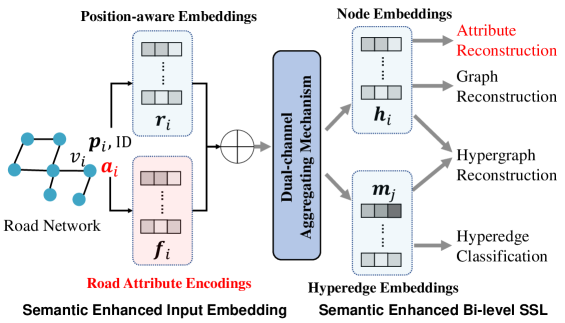
When road attributes are available, we propose to extend HyperRoad by introducing road attributes into embedding layer and adding an auxiliary road attribute reconstruction task following the same encoder-decoder strategy as for modeling structural information. We name this advanced model as HyperRoad-A, and an overview of its framework is given in Fig. 4 (with the newly added components highlighted in red).
Semantic Enhanced Input Embedding. In the encoder part, we model road attributes as another kind of semantic input information besides road ID and position. For a target road , the new input embedding is defined as , where is the original input embedding of HyperRoad defined in Section 3.1 and is the embedding of ’s road attributes via one-hot encoding.
Semantic Enhanced Self Supervised Learning. To force the learned road representations preserve the semantic/attribute information, we add another auxiliary attribute reconstruction task in the self supervised learning module. Specifically, given a road and its attributes , we aim at predicting these attributes based on the learned representation with the additional loss defined as follows.
| (13) |
where is the number of road attributes, is the number of possible values for the -th attribute , is the -th dimension of an output vector obtained by transforming the road representation as , and equal to 1 when is equal to the attribute value and 0 otherwise.
Then, the joint learning loss function for HyperRoad-A can be defined as follows.
| (14) |
4.2. HyperRoad-T: with Additional Trajectories
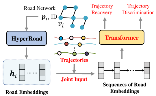
Traveling patterns serve as a generic feature on road networks, which should be properly integrated so that they can precisely enrich the multi-faced knowledge about road networks such as underlying functional characteristics (wu2020learning, 36, 2). In the section, we extend HyperRoad to the setting, where some trajectories on a road network are available. We call the resulting model HyperRoad-T. The overview of the HyperRoad-T framework is shown in Fig. 5, where we follow a pre-training and refining strategy (with the newly added components highlighted in red).
In the first stage, we train the road representations by optimizing the loss function defined in Equation 12. Then, these representations are treated as the input embeddings of a stacked bidirectional transformer. Following existing work (chen2021robust, 2), we adopt two BERT-style self supervised learning tasks, i.e., trajectory recovery and trajectory discrimination to help trajectory modeling.
Trajectory Recovery. Similar to the MLM (Masked Language Model) task used in BERT, we mask a sequence of consecutive roads to form a partially observed route given a trajectory. The transformer is then trained to predict these masked roads.
Trajectory Discrimination. Similar to the NSP (Next Sentence Prediction) task used in BERT, we adopt a trajectory level task besides the token level recovery task. Specifically, we sample real trajectories from trajectory database and generate fake trajectories through random walks on road network. This task is to judge whether a given road sequence is a real human trajectory or not.
4.3. HyperRoad-AT: with Additional Attributes and Trajectories
We further extend HyperRoad for the setting with additional road attributes and trajectories. Specifically, it corresponds to the HyperRoad-T model, with the HyperRoad component replaced by HyperRoad-A. That is, we first pre-train the attribute aware road representation by base model HyperRoad-A, and then finetune road embeddings through trajectory modeling following the same strategy in Section 4.2. We call the resulting model HyperRoad-AT.
5. Experimental Setup
In order to evaluate the effectiveness of our proposed model HyperRoad and its extensions, we conduct extensive experiments to answer the following questions.
RQ1: Can HyperRoad outperform other models on the downstream tasks when only structural and spatial information of a road network is available (the default setting)?
RQ2: What roles do different components of HyperRoad play in improving the model performance?
RQ3: How would different hyper-parameters influence the performance of HyperRoad?
RQ4: What do the learned road embeddings represent? Can these embeddings capture the underlying characteristics of road networks?
RQ5: Can the extensions of HyperRoad outperform the state-of-the-art models when additional attributes and/or trajectories are available?
In this section, we first describe the experimental settings.
| Setting | Baselines | Our Model | |||
|
|
HyperRoad | |||
| + Road Attributes |
|
HyperRoad-A | |||
| + Trajectory |
|
HyperRoad-T | |||
| + Attributes & Trajectory |
|
HyperRoad-AT |
5.1. Baseline models
We compare our model with the following 9 baselines, as described as follows.
-
•
Node2Vec (grover2016node2vec, 5), LINE (tang2015line, 27), SDNE (wang2016structural, 32), GAE (kipf2016variational, 15), and GraphSAGE (hamilton2017inductive, 7): The former three are traditional graph representation learning models and the latter two are GNN-based graph representation learning models. They are compared under the default setting since they are all general graph structure representation learning methods.
-
•
RFN (jepsen2020relational, 11): RFN uses both primal and dual graphs to model road networks where roads are considered edges in the primal graph and nodes in the dual graph. The road representations are learned by fusing two views’ information to a graph auto-encoder framework.
We consider two versions, RFN and RFN-A. In RFN, we use the proposed position-aware embeddings as model input. In RFN-A, we further incorporate the road attribute embedding as input. Note that it is non-trivial to extend the RFN model with additional inputs of trajectories.
-
•
IRN2Vec (wang2019learning, 33): IRN2Vec applies shortest path sampling and skip-gram model to predict the information of geo-locality, geo-shape, and road tags given road sequences. We consider two versions, IRN2Vec and IRN2Vec-A. In IRN2Vec, we exclude the tag-based loss function, and in IRN2Vec-A, we follow the setting of the original paper (wang2019learning, 33). Note that it is non-trivial to extend the IRN2Vec model with additional inputs of trajectories.
-
•
HRNR (wu2020learning, 36): It learns road representation by preserving road network semantic and traffic information in a hierarchical manner. The attributes are used as a part of input embedding and trajectories are used as a extra loss function. We consider four versions of HRNR, namely HRNR, HRNR-A, HRNR-T, and HRNR-AT. In HRNR, we use the position-aware embeddings as model input and exclude the trajectory-based loss function. In HRNR-A, we further incorporate the road attribute embedding as inputs. In HRNR-T, we add the trajectory-based loss function. Finally, in HRNR-AT, we combine HRNR-A and HRNR-T.
-
•
Toast (chen2021robust, 2): It utilizes auxiliary traffic attributes to train a skip-gram model. Specifically, a trajectory-enhanced Transformer module is utilized to extract traveling semantics on trajectory data. We consider four versions of Toast, namely Toast, Toast-A, Toast-T, and Toast-AT. In Toast, we exclude the attribute prediction task and trajectory-enhanced module (this would degrade to the DeepWalk model). In Toast-A, we add the auxiliary attributes in skip-gram model. In Toast-T, we add the trajectory-enhanced module. Finally, in Toast-AT, we combine Toast-A and Toast-T.
A summary of baseline models under different settings is provided in Table 1. For fair comparison, we incorporate the position-aware embeddings to those GNN based baseline models, including HRNR, GAE, GraphSAGE, and RFN (these studies do not consider node position information by default), so that they take the same inputs as our model HyperRoad. Among other baseline models, IRN2Vec uses spatial information as supervision signals and the rest models do not use the spatial information and it remains non-trivial to incorporate the spatial information to these models. Note that following the existing works (jepsen2020relational, 11, 33, 36), we do not consider the specialized models such as (pan2019urban, 23, 17, 40) which are designed for a specific task as baselines, because our goal is to evaluate the usefulness and generalization of the learned road representations. These specialized methods are highly dependent on the task-specific model designs and usually take more data as input and it would not be fair to compare our model with these methods. Therefore we use the same task-specific components and make them as simple as possible for all the compared RNRL models.
5.2. Evaluation Tasks
We consider two types of downstream tasks, namely road based and trajectory based tasks, for evaluation. For each task, we employ a simple task-specific component (e.g., LSTM or Logistic Regression) with the learned road network representations as input. We exploit the same task-specific component for all compared models for fair comparison. The adopted tasks are described as follows.
Road based tasks. Following the existing work (yin2021multimodal, 41), we consider the following four important road attribute predictions as road based tasks: 1) one/two way classification, 2) lanes classification, 3) speed limit classification, and 4) road type classification. For each task, we choose the road attribute values as the labels, regard the learned road representations as input features, and use an one-vs-rest logistic regression classifier to make predictions.
Trajectory based tasks. Following the existing work (wang2019learning, 33), we use travel time estimation task as the trajectory based task. Travel time estimation is a regression task, which predicts the travel time of a given moving path in road networks. We apply a simple Long Short-Term Memory (LSTM) layer followed by one fully-connected layer as the regression model, which takes the road representation as input and outputs the estimated travel time.
Remarks. When considering road attributes as extra information, we use one/two way, lanes and speed limit as road attributes, and only treat the road type classification as road based task to avoid data leakage.
5.3. Datasets, Evaluation Metrics and Parameter Settings
Datasets. We use the road networks of two cities, Singapore and Xi’an, in our experiments. The structural and spatial information and the road attributes are collected from OpenStreetMap. The trajectories are obtained from public datasets released by Grab and DiDi Chuxing for Singapore and Xi’an, respectively. In trajectories, the raw GPS points are transformed by map matching (yang2018fast, 39) into road sequences. The statistics of these datasets are shown in Table 2.
Evaluation Metrics. For road based tasks, we adopt Micro-F1, Macro-F1 and Weighted-F1 to evaluate the classification accuracy, and for the trajectory based task (travel time estimation), we adopt MAE (Mean Average Error) and RMSE (Root Mean Square Error) to evaluate the regression accuracy.
Remarks. For all the mentioned tasks, we apply 5-fold cross validation to evaluate the performance of all the methods. For example, for the road based tasks, we use 4-fold road representations and their tag labels as training data and use the rest 1-fold data as test set (we also randomly sampled 10% of each training fold to act as a validation set during training process). We report the average of the results of 5-fold test sets.
Parameter Settings. In our experiments, we set the embedding dimension to be 64 for all the models for fair comparison. For random walk based methods such as Node2Vec, IRN2Vec and Toast, the walk length and the window size are set to be 20 and 5 respectively. The number of walks per node are searched in {30, 50, 80}. The parameters and for Node2Vec are tuned in {0.25, 0.5, 1.0, 2.0}. We use half dimensions for first-order proximity and another half for second-order proximity in LINE. The encoder and decoder are implemented as a two-layer MLP with hidden dimensions of {1024, 64} for SDNE. The aggregation layers are selected from {2, 3, 4} for all the GNN-based methods. For HyperRoad, We use a mini-batch Adaptive Moment Estimation (Adam) (kingma2015adam, 13) optimizer. The learning rate and batch size are set to be 0.001 and 1,024 respectively. The scale parameter and frequency parameter in Equation 1 are set to be 10 and 1,000 separately. The weighted parameter in the loss function is set to be 0.1 for both datasets. The negative sizes for graph sampling and hypergraph sampling named and are set to be 5 and 2. The number of hyperedge clusters are set to be 8 and 7 for Singapore dataset and Xi’an dataset, respectively. We also tune the number of layers for the dual-channel aggregating mechanism in the set of {2,3,4}. Further, in HyperRoad-A, the weight for loss is set to be 1.0. In HyperRoad-T and HyperRoad-AT, 2 multi-head self-attention layers are stacked and the head number is set as 4.
The codes and datasets can be found via this link 111https://drive.google.com/drive/folders/1oz19-F0igSziViKU4qmhDH-Do1Oudrh_?usp=sharing. We implement HyperRoad using PyTorch (paszke2019pytorch, 24). Our software environment contains Ubuntu 18.04.3, PyTorch 1.2.0 and python 3.7.3. All of the experiments are conducted on a machine with 2 GPUs (Tesla V100-SXM2 * 2), 20 CPUs (Inter i7 6850K) and 500G memories.
| Dataset | Singapore | Xi’an |
| # Roads | 33,948 | 53,067 |
| # Edges | 147,550 | 249,848 |
| # Hyperedges | 3,772 | 6,953 |
| # Trajectories | 28,000 | 50,000 |
| # One/Two Way | 2 | 2 |
| # No. of Lanes | 6 | 6 |
| # Speed Limit | 6 | 9 |
| # Road Type | 5 | 5 |
6. Experimental Results
| Model | One/Two Way | No. of Lanes | ||||||||||
| Singapore | Xi’an | Singapore | Xi’an | |||||||||
| Micro-F1 | Macro-F1 | Weighted-F1 | Micro-F1 | Macro-F1 | Weighted-F1 | Micro-F1 | Macro-F1 | Weighted-F1 | Micro-F1 | Macro-F1 | Weighted-F1 | |
| Node2Vec | 0.7213 | 0.4221 | 0.6059 | 0.5858 | 0.5638 | 0.5743 | 0.4773 | 0.1077 | 0.3087 | 0.5600 | 0.2675 | 0.4789 |
| LINE | 0.7652 | 0.6018 | 0.7117 | 0.6032 | 0.5909 | 0.5985 | 0.4772 | 0.1094 | 0.3101 | 0.5504 | 0.1900 | 0.4070 |
| SDNE | 0.7199 | 0.4226 | 0.6058 | 0.5686 | 0.5114 | 0.5295 | 0.4778 | 0.1117 | 0.3120 | 0.5504 | 0.1833 | 0.3998 |
| GAE | 0.7135 | 0.4935 | 0.6342 | 0.6676 | 0.6650 | 0.6677 | 0.4790 | 0.1248 | 0.3186 | 0.5827 | 0.3383 | 0.5235 |
| GraphSAGE | 0.7170 | 0.4829 | 0.6296 | 0.6452 | 0.6398 | 0.6438 | 0.4793 | 0.1228 | 0.3170 | 0.5794 | 0.2990 | 0.5181 |
| RFN | 0.7410 | 0.5995 | 0.6990 | 0.6305 | 0.6213 | 0.6267 | 0.4784 | 0.1177 | 0.3154 | 0.5596 | 0.2757 | 0.4737 |
| IRN2Vec | 0.7085 | 0.4538 | 0.6110 | 0.6274 | 0.6100 | 0.6175 | 0.4793 | 0.1271 | 0.3190 | 0.5677 | 0.2176 | 0.4508 |
| HRNR | 0.7226 | 0.6379 | 0.7145 | 0.6659 | 0.6606 | 0.6652 | 0.4767 | 0.1076 | 0.3078 | 0.5601 | 0.2957 | 0.4547 |
| Toast | 0.7313 | 0.5027 | 0.6517 | 0.5888 | 0.5647 | 0.5758 | 0.4766 | 0.1082 | 0.3089 | 0.5498 | 0.2009 | 0.4209 |
| HyperRoad | 0.7864 | 0.6995 | 0.7676 | 0.7051 | 0.7033 | 0.7054 | 0.4829 | 0.1534 | 0.3392 | 0.5955 | 0.3670 | 0.5459 |
| Improvement | 2.77% | 9.66% | 7.43% | 5.62% | 5.76% | 5.66% | 0.75% | 20.69% | 6.33% | 2.20% | 8.48% | 4.28% |
| Model | Speed Limit | Road Type | ||||||||||
| Singapore | Xi’an | Singapore | Xi’an | |||||||||
| Micro-F1 | Macro-F1 | Weighted-F1 | Micro-F1 | Macro-F1 | Weighted-F1 | Micro-F1 | Macro-F1 | Weighted-F1 | Micro-F1 | Macro-F1 | Weighted-F1 | |
| Node2Vec | 0.5782 | 0.1273 | 0.4252 | 0.7661 | 0.7620 | 0.7679 | 0.4984 | 0.2733 | 0.4590 | 0.3791 | 0.2680 | 0.3298 |
| LINE | 0.5781 | 0.1221 | 0.4235 | 0.5920 | 0.6669 | 0.5917 | 0.5059 | 0.2715 | 0.4638 | 0.3892 | 0.2674 | 0.3358 |
| SDNE | 0.5766 | 0.1235 | 0.4243 | 0.4825 | 0.4288 | 0.4546 | 0.4806 | 0.2594 | 0.4422 | 0.3653 | 0.2270 | 0.2940 |
| GAE | 0.5944 | 0.1980 | 0.4654 | 0.7661 | 0.8393 | 0.7636 | 0.5017 | 0.3462 | 0.4762 | 0.4321 | 0.3744 | 0.4097 |
| GraphSAGE | 0.5910 | 0.1864 | 0.4558 | 0.7711 | 0.8500 | 0.7700 | 0.4955 | 0.3238 | 0.4648 | 0.4312 | 0.3715 | 0.4086 |
| RFN | 0.5904 | 0.1579 | 0.4471 | 0.6368 | 0.6711 | 0.6321 | 0.5260 | 0.3207 | 0.4877 | 0.4031 | 0.2937 | 0.3547 |
| IRN2Vec | 0.5869 | 0.1479 | 0.4341 | 0.6119 | 0.5444 | 0.5962 | 0.4773 | 0.2567 | 0.4353 | 0.3836 | 0.2924 | 0.3475 |
| HRNR | 0.5868 | 0.1232 | 0.4341 | 0.6915 | 0.6052 | 0.6852 | 0.5050 | 0.2585 | 0.4399 | 0.4485 | 0.3155 | 0.3914 |
| Toast | 0.5784 | 0.1231 | 0.4245 | 0.5820 | 0.5727 | 0.5814 | 0.4987 | 0.2697 | 0.4581 | 0.3697 | 0.2491 | 0.3139 |
| HyperRoad | 0.6066 | 0.2534 | 0.4970 | 0.7861 | 0.8566 | 0.7832 | 0.5785 | 0.3964 | 0.5482 | 0.4562 | 0.3957 | 0.4359 |
| Improvement | 2.05% | 27.98% | 6.79% | 1.95% | 0.78% | 1.71% | 9.98% | 14.50% | 12.41% | 1.72% | 5.69% | 6.39% |
6.1. Performance Comparison (RQ1)
We first evaluate the learned embeddings in the road based tasks. We show the performances of different models in Table 3, where the best performance is in boldface and the second best is underlined. From the results, we have the following observations. First, the performances of GNN-based models are generally much better than traditional graph representation learning models, showing the advantages of deep neural networks in road network structure modeling over shallow representations. Second, the performances of road network representation learning models are the best in many cases among the baselines. For example, HRNR tends to perform better on one/two way prediction while RFN is better on road type classification task. However, the simple graph reconstruction objective of RFN and HRNR hinder their performance and superiority on other downstream applications. Third, our model performs consistently better than all the baselines in terms of all the metrics on the four tasks. And the average margin in Macro-F1 reaches 18.20% and 5.18% for Singapore and Xi’an dataset respectively. It shows that HyperRoad can better capture the underlying characteristics of road networks with help of the newly neighborhood aggregation mechanism and auxiliary hypergraph-level pre-training task.
Next, we discuss the model performance on travel time estimation task in Table 4. It can be observed that HyperRoad consistently outperforms all competitors on both datasets. The result demonstrates that the road embeddings learned by HyperRoad can also be applicable for traffic level tasks. A possible reason is that the travel time is highly related to road information such as road type and road speed. HyperRoad captures the intrinsic properties of the road networks and thus improve the task performance. It verifies the effectiveness of the learned road representations from another perspective.
| Model | Singapore | Xi’an | ||
| MAE | RMSE | MAE | RMSE | |
| Node2Vec | 152.44 | 219.29 | 272.54 | 390.06 |
| LINE | 153.84 | 220.88 | 276.71 | 396.77 |
| SDNE | 162.43 | 231.80 | 277.62 | 397.26 |
| GAE | 152.07 | 225.33 | 271.43 | 388.73 |
| GraphSAGE | 151.83 | 219.88 | 272.22 | 390.90 |
| RFN | 154.76 | 219.70 | 273.35 | 395.48 |
| IRN2Vec | 151.45 | 218.06 | 281.89 | 398.86 |
| HRNR | 168.35 | 244.09 | 275.62 | 397.22 |
| Toast | 158.72 | 230.61 | 272.12 | 395.05 |
| HyperRoad | 145.79 | 214.39 | 266.50 | 382.25 |
| Improvement | 3.73% | 1.68% | 1.82% | 1.67% |
| Model | One/Two Way | No. of Lanes | Speed Limit | Road Type | ||||||||
| Micro-F1 | Macro-F1 | Weighted-F1 | Micro-F1 | Macro-F1 | Weighted-F1 | Micro-F1 | Macro-F1 | Weighted-F1 | Micro-F1 | Macro-F1 | Weighted-F1 | |
| w/o PE | 0.7690 | 0.6619 | 0.7421 | 0.4762 | 0.1092 | 0.3091 | 0.5880 | 0.1324 | 0.4420 | 0.5756 | 0.3193 | 0.5301 |
| w/o DAM | 0.7545 | 0.6221 | 0.7164 | 0.4784 | 0.1183 | 0.3145 | 0.5929 | 0.1928 | 0.4544 | 0.5497 | 0.3609 | 0.5114 |
| AM-KGNN | 0.7832 | 0.6903 | 0.7618 | 0.4768 | 0.1174 | 0.3148 | 0.5897 | 0.1555 | 0.4447 | 0.5587 | 0.3022 | 0.5117 |
| DAM-ATT | 0.7434 | 0.6079 | 0.7051 | 0.4807 | 0.1339 | 0.3257 | 0.5888 | 0.2001 | 0.4600 | 0.5496 | 0.3789 | 0.5203 |
| DAM-MLP | 0.7773 | 0.6802 | 0.7545 | 0.4808 | 0.1395 | 0.3295 | 0.5945 | 0.1997 | 0.4653 | 0.5667 | 0.3350 | 0.5255 |
| w/o GPT | 0.7804 | 0.6875 | 0.7593 | 0.4793 | 0.1403 | 0.3293 | 0.5876 | 0.1952 | 0.4568 | 0.5742 | 0.3466 | 0.5316 |
| w/o HPT | 0.7402 | 0.5965 | 0.6980 | 0.4827 | 0.1465 | 0.3327 | 0.6016 | 0.2341 | 0.4885 | 0.5220 | 0.3598 | 0.4937 |
| w/o HEC | 0.7239 | 0.5442 | 0.6648 | 0.4794 | 0.1287 | 0.3243 | 0.5945 | 0.1602 | 0.4572 | 0.5553 | 0.3679 | 0.5217 |
| HyperRoad-DBS | 0.7879 | 0.7017 | 0.7693 | 0.4796 | 0.1497 | 0.3371 | 0.5962 | 0.2277 | 0.4838 | 0.5724 | 0.3674 | 0.5349 |
| HyperRoad | 0.7864 | 0.6995 | 0.7676 | 0.4829 | 0.1534 | 0.3392 | 0.6066 | 0.2534 | 0.4970 | 0.5785 | 0.3964 | 0.5482 |
6.2. Ablation Study (RQ2)
In this section, we perform ablation studies on Singapore dataset to inspect how each module of HyperRoad affects the model performance in four downtream tasks.
There are three core modules in HyperRoad: positional encoding, dual-channel aggregation mechanism, self-supervised learning with both graph-level and hypergraph-level pretext tasks. By removing or replacing these modules, we can obtain different variants of HyperRoad. Specifically, we firstly remove the positional encoding module in the model variant w/o PE. Then, we remove the dual-channel aggregation mechanism and obtain the model variant w/o DAM, in which we only use the hyperedge channel aggregation to update the road representations. Note that we do not consider the case of using edge channel aggregation only, since it can not update and output the hyperedge representations necessary for subsequent hypergraph-level objectives. Considering the effectiveness of the newly proposed high-order graph neural networks (morris2019weisfeiler, 22) in capturing high-order node relations, we replace the dual-channel aggregation mechanism with k-GNN in (morris2019weisfeiler, 22) and name this model variant as AM-KGNN. In addition, to better validate the design of dual-channel aggregation, we use attention and MLP aggregators to implement in channel fusion and obtain two models named DAM-ATT and DAM-MLP respectively. Finally, models w/o GPT and w/o HPT can be obtained by removing the corresponding graph-level pretext task and hypergraph-level pretext task. To verify the importance of the newly proposed hyperedge classification task in road network, we obtain another model variant w/o HEC where only the hyperedge classification task is removed. To investigate the impacts of negative sampling methods, we replace the random sampling process with a distance based sampling (DBS) process and obtain a model variant called HyperRoad-DBS. Here, in the distance based sampling process, the sampling probability of a candidate road in is defined as the normalization of its shortest path distance from the anchor road . The sampling probability for a candidate hyperedge in is defined using the same strategy, where the distance between and is the average of shortest path distances between roads in and . The ablation results are shown in Table 5.
Contribution of the positional encoding. By comparing w/o PE and HyperRoad, we can find that the positional encoding module indeed brings substantive improvement in downstream task performances. For example, HyperRoad outperforms the base model w/o PE by 40.42% in Macro-F1 on average. The results justify the fact that the geo-location information is the core property of road network, and it can hardly be captured only by the graph structures.
Contribution of the dual-channel aggregation mechanism. The main difference between HyperRoad and w/o DAM is whether to aggregate information from two channels named edge channel and hyperedge channel at the same time. As seen from Table 5, HyperRoad brings at least 9.83% improvement in terms of Macro-F1 compared with w/o DAM. This is because the two channels capture different graph structure information. Using only one of them will cause information loss and lead to inferior model performance. In addition, although AM-KGNN aggregates the information from high-order neighbors defined by the -order cliques, these different structures are still defined on the same simple graph. The results demonstrate the importance of our proposed dual channel aggregation mechanism. As for different channel fusion operations, the simple mean aggregation (adopted in HyperRoad) can achieve the best results. A possible reason might be that the extra MLP or attention layer introduces too much non-linearity for road representation learning, which is hard to train.
Contribution of the self-supervised pretext tasks. By comparing the performance of w/o GPT, w/o HPT, w/o HEC, HyperRoad-DBS and HyperRoad, we have the following observations. 1) HyperRoad which considers both graph-level and hypergraph-level tasks generally has better performance than the models considering only single aspect, i.e., w/o GPT and w/o HPT. The result demonstrates that both level tasks are important for effective road representations. 2) The model w/o GPT performs better on one/two way classifications while w/o HPT is better on speed limit predictions. From another perspective, it verifies that each level task has its own merit to enhance the road representations. 3) Model w/o HEC simply combines two commonly used reconstruction tasks, namely graph reconstruction and hypergraph reconstruction. Compared with w/o HPT which only applies the graph reconstruction task, w/o HEC performs better for Road Type prediction but performs worse for other applications. The results verify the advantages of introducing the hypergraph reconstruction task to RNRL. It also demonstrates that simply combining two commonly used reconstruction tasks may introduce noise for model learning. In contrast, HyperRoad achieves the best performance for all applications, showing the benefit of the newly proposed hyperedge classification task. 4) As for different sampling methods, the random sampling model (adopted in HyperRoad) achieves better performances than the distance based sampling method. A possible reason is that roads far away on the map may still serve as similar urban functions and it is unreasonable to treat them as negative samples more frequently as HyperRoad-DBS does. This results also verify the importance of long-range relationship in road network from another perspective.
6.3. Parameter Sensitivity (RQ3)
We conduct the parameter study on the weighted parameter , the embedding size , and the number of layers on our example dataset Singapore as follows. Fig. 6 shows the model performance in terms of Macro-F1 under different settings.
The weighted parameter . Generally, the model performances first increase along with , and then begin to drop when is larger than 0.1. It is worth mentioning that HyperRoad would reduce to w/o HPT when is zero, and to w/o GPT when is infinity. The discovered trend conforms to the their performances in ablation study and again shows the necessity of introducing both self-supervised learning tasks.
The embedding size . The model performances increase with embedding size in most cases, since large embedding size tends to have stronger representational power. However, using high-dimensional representation does not always produce the best results. For example, the Macro-F1 achieves the best when rather than on road type classification.
The number of layers . The model performances remain relatively stable when increases, and the best results for all application tasks can be achieved when . The model performance at is slightly worse than that of , showing potential for overfitting and oversmoothing.


6.4. Case Study for Representation Understanding (RQ4)
In this section, we use auxiliary information such as road attributes to help uncover what HyperRoad has learned. Note that these information is not available for model training in our default problem setting.
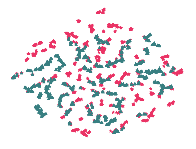
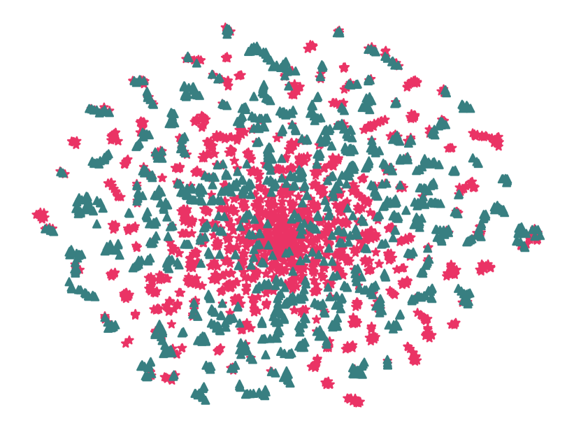
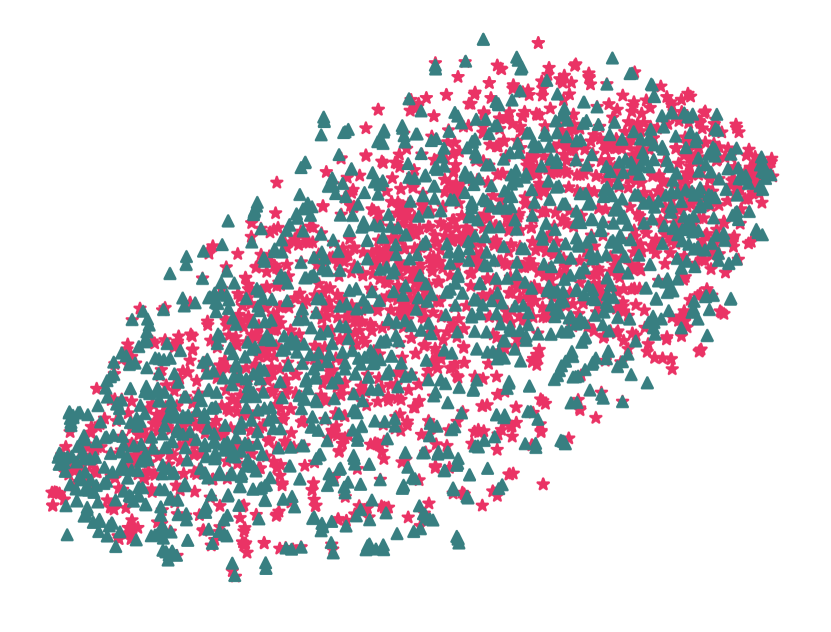
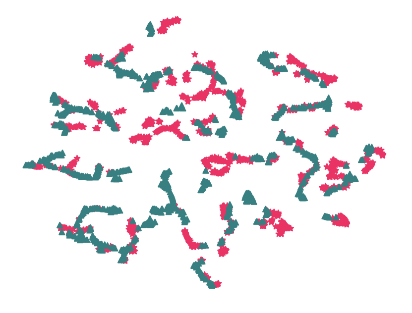
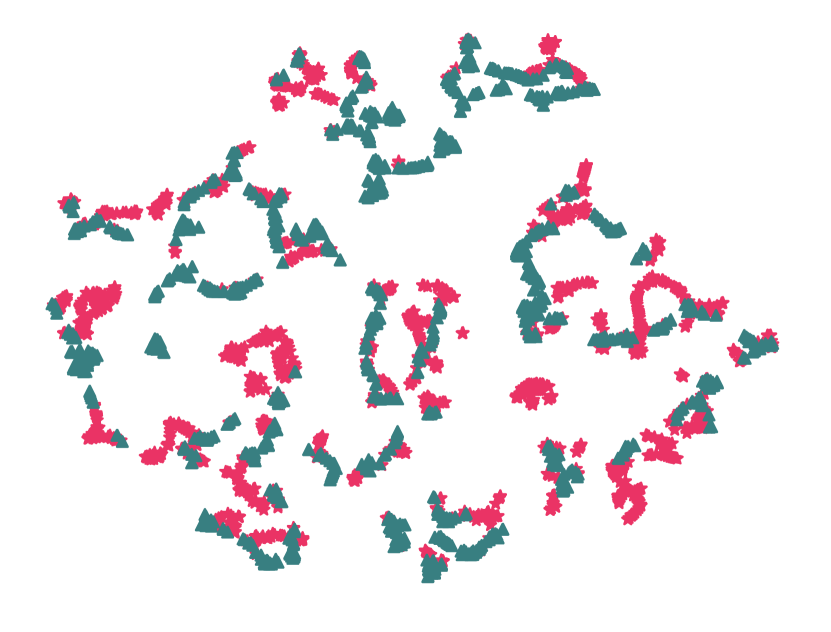
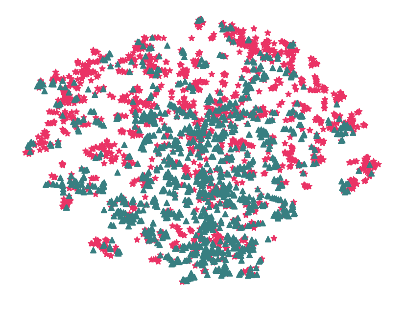
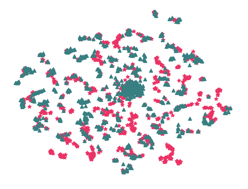
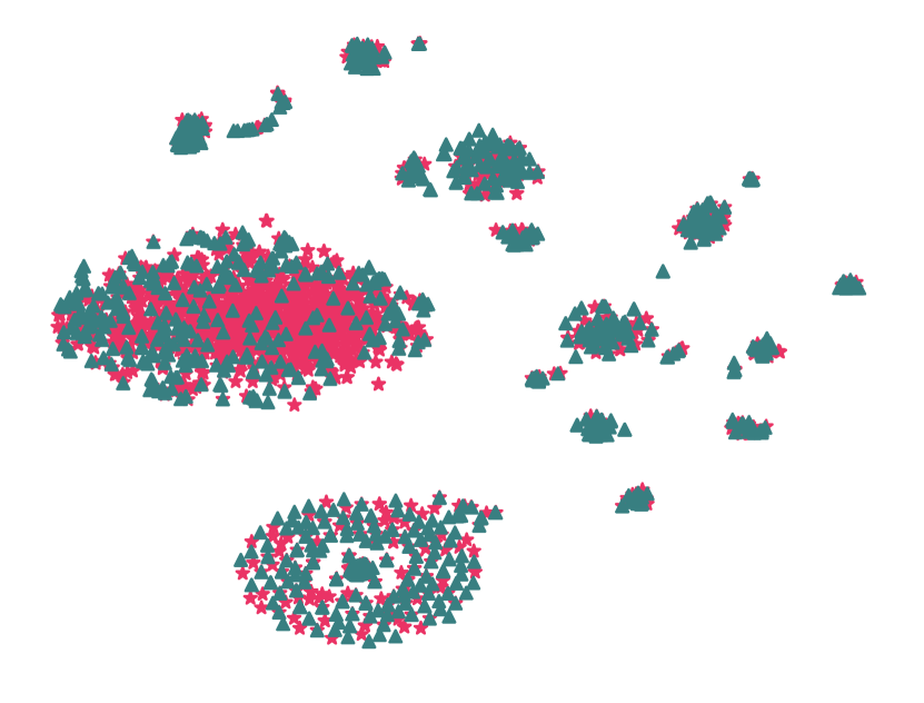
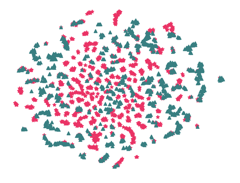
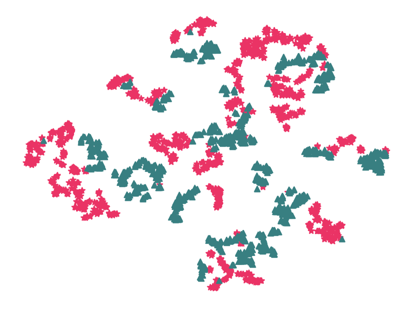
We first exploit the network visualization approach to evaluate node embeddings learned by different models. Here, we take a rectangular region of Singapore as an example. The longitude is between and , and the latitude is between and . Then, we select roads located in this region and employ the t-SNE model (van2008visualizing, 29) to project road embeddings to a 2-dimensional space. For the sake of visualization, we present the results for two road types with different semantics namely motorway and residential. The projected results of different models are shown in Fig. 7. From the results, we make the following observations. 1) The shallow network representation models failed to separate the two road types clearly. For example, in Node2Vec and IRN2Vec, two road types are mixed together in the middle of Fig. 7(a) and Fig. 7(g). The reason is that random walks may not preserve the node homogeneity, and thus lead to similar representations for roads with different semantics. 2) There are different clusters in the results of HRNR as shown in Fig. 7(h). This is because HRNR is a hierarchical GNN structure, and each node can aggregate information from too many neighbors through the hidden nodes. This aggregation mechanism leads to the oversmoothing problem. 3) RFN, GraphSAGE and GAE provide more reasonable visualizing results. However, some clusters are still mixed with each other and there is no clear margin between different classes. 4) In contrast, HyperRoad gives the most satisfying identification with relatively clear cluster boundaries. The reason is that the proposed dual-channel aggregation mechanism can help the model to find high-order neighbors with similar semantics, and the hypergraph-level tasks provides extra prior knowledge for road representation learning.
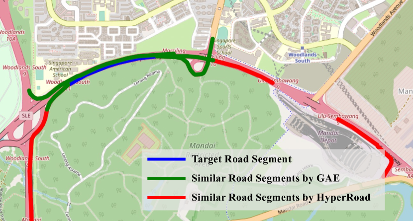
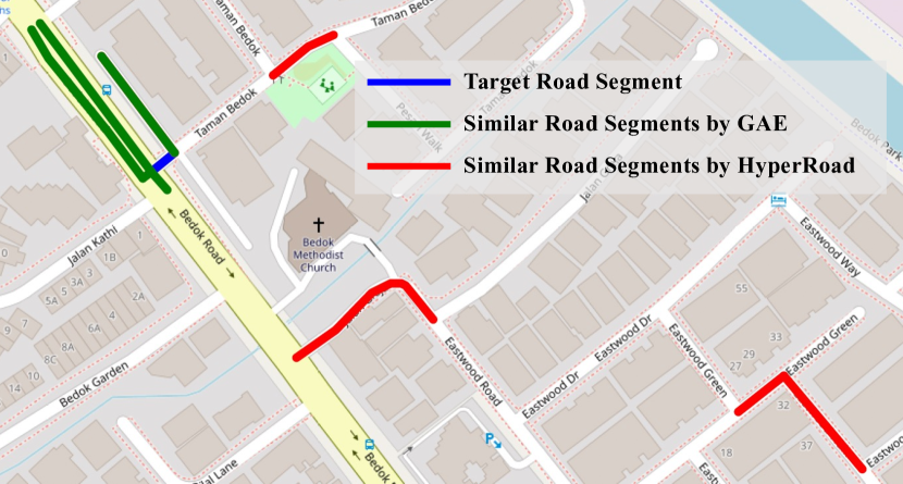
We further pick two specific cases to explain the road embeddings learned by different models in details. GAE is selected as a reference model given its satisfactory task performances and visualizing results. Specifically, we first randomly sample two roads and with distinct semantic information as target roads. For each road, we extract its top 5 most similar roads in GAE and HyperRoad with cosine similarity. The road attributes are shown in Table 6 and the geo-locations are plotted in Fig. 8. It is clear to see that GAE mainly recalls very close neighbors in geo-space although their attributes are significantly different. For example, the motorways are considered similar to residential roads in case two. The results show that the adopted graph reconstruction objective in GAE is not effective in modeling complex road networks. In contrast, our model captures both location and semantic information together for querying similar roads. For example, in both case one and case two, our model can find the roads with quite similar functions in a reasonable long range, which justifies the necessity of the proposed hypergraph modeling.
| Category | Case One | Case Two | |||||||||||||||||||||||
| ID |
|
|
|
|
ID |
|
|
|
|
||||||||||||||||
| Target road | one way | 3 | 90 | motorway | two way | 2 | 50 | residential | |||||||||||||||||
| Similar roads by GAE | one way | 4 | 90 | motorway | two way | 2 | 50 | residential | |||||||||||||||||
| one way | 3 | 90 | motorway | one way | 1 | 50 | motorway | ||||||||||||||||||
| one way | 2 | 50 | motorway | one way | 1 | 50 | motorway | ||||||||||||||||||
| one way | 2 | 50 | motorway | one way | 1 | 50 | motorway | ||||||||||||||||||
| one way | 1 | 50 | motorway | one way | 1 | 50 | motorway | ||||||||||||||||||
| Similar roads by HyperRoad | one way | 3 | 90 | motorway | two way | 2 | 50 | residential | |||||||||||||||||
| one way | 3 | 90 | motorway | two way | 2 | 50 | residential | ||||||||||||||||||
| one way | 4 | 90 | motorway | two way | 2 | 50 | residential | ||||||||||||||||||
| one way | 4 | 90 | motorway | two way | 2 | 50 | residential | ||||||||||||||||||
| one way | 4 | 70 | motorway | two way | 2 | 50 | residential | ||||||||||||||||||
6.5. Extensions to Other Settings (RQ5)
In this section, we study road type classification task (by excluding the road type attributes in the inputs) and the travel time estimation task on the Singapore dataset. The model performances under various settings are shown in Table 7. Based on the results, we have the following observations.
Comparisons among problem settings. In general, including additional inputs can help to learn better road network representations. For example, HyperRoad-AT significantly exceeds its counterpart HyperRoad with relative improvements of 33.5% and 11.2% in terms of Macro-F1 and RMSE, respectively. Similar findings can also be witnessed by comparing any extended model with its base model. In addition, we find that using road attributes is more effective for road type classification, while using trajectory is more effective for travel time estimation.
Comparisons among models. By comparing the performances of HyperRoad extensions with other baseline models, we can find that the proposed model achieves the best results on two tasks across all the settings studied. For example, HyperRoad-AT outperforms the best baseline Toast-AT by 16.8% in terms of Macro-F1 on road type classification task.
| + Attributes | Road Type Classification | Travel Time Estimation | |||
| Micro-F1 | Macro-F1 | Weighted-F1 | MAE | RMSE | |
| RFN-A | 0.7264 | 0.4606 | 0.6919 | 152.20 | 211.16 |
| IRN2Vec-A | 0.5054 | 0.2732 | 0.4628 | 150.44 | 210.99 |
| HRNR-A | 0.6776 | 0.3670 | 0.6212 | 165.21 | 232.26 |
| Toast-A | 0.7353 | 0.4254 | 0.6792 | 155.06 | 208.78 |
| HyperRoad-A | 0.7497 | 0.5166 | 0.7110 | 145.67 | 205.69 |
| Improvement | 1.96% | 12.16% | 2.76% | 3.17% | 1.48% |
| + Trajectory | Road Type Classification | Travel Time Estimation | |||
| Micro-F1 | Macro-F1 | Weighted-F1 | MAE | RMSE | |
| HRNR-T | 0.5989 | 0.3244 | 0.5492 | 155.12 | 213.22 |
| Toast-T | 0.6210 | 0.3364 | 0.5695 | 144.44 | 205.18 |
| HyperRoad-T | 0.6327 | 0.4294 | 0.5994 | 141.28 | 195.42 |
| Improvement | 1.88% | 27.65% | 5.25% | 2.19% | 4.76% |
| + Attributes & Trajectory | Road Type Classification | Travel Time Estimation | |||
| Micro-F1 | Macro-F1 | Weighted-F1 | MAE | RMSE | |
| HRNR-AT | 0.7060 | 0.3823 | 0.6473 | 154.98 | 208.87 |
| Toast-AT | 0.7512 | 0.4533 | 0.6996 | 142.23 | 199.52 |
| HyperRoad-AT | 0.7621 | 0.5294 | 0.7233 | 137.93 | 189.39 |
| Improvement | 1.45% | 16.79% | 3.39% | 3.03% | 5.08% |
7. Related Work
Road Networks Modeling and Representation Learning. Road network has been used in various applications, such as traffic inference and forecasting (hu2019stochastic, 9, 6), road tags prediction (yin2021multimodal, 41), and region functionality modeling (wozniak2021hex2vec, 35). In this studies, road embeddings are indirectly learned as a byproduct to incorporate structural and spatial information. However, the methods in these studies are tailored for specific tasks, and the representations learned for one task can hardly be transferred to other tasks. Recently, a few studies propose to learn generic road representations by extending graph representation learning to road networks (jepsen2020relational, 11, 33, 36, 2). In specific, IRN2Vec (wang2019learning, 33) extends the skip-gram model by considering geo-locality and geo-shape information. Toast (chen2021robust, 2) extends skip-gram model by adding auxiliary attributes prediction task and trajectory-enhanced transformer module. RFN (jepsen2020relational, 11) and HRNR (wu2020learning, 36) extend GCN by considering dual node-relational and edge-relational views and hierarchical graph structures respectively. However, none of these methods are sufficient in capturing the high-order relationships and long-range relationships, as has been explained in Section 1.
Graph Representation Learning. Recent years have witnessed the great success of graph representation learning. The earliest efforts in this field mainly focus on shallow representations. For example, DeepWalk (perozzi2014deepwalk, 25) and Node2Vec (grover2016node2vec, 5) use random walks on the graph to generate node sequences and then apply skip-gram model (mikolov2013distributed, 21) to learn node representations. LINE (tang2015line, 27) aims to preserve the first and second-order proximities by explicitly modeling the corresponding objectives. All these models are actually equivalent to the simple matrix factorization framework with closed forms (qiu2018network, 26). Inspired by the recent huge success of deep learning, graph neural networks have been introduced for graph representation learning. Along this line, graph convolution networks (GCN) (kipf2016semi, 14) and graph attention network (GAT) (velivckovic2017graph, 31) are two classic models. These GNN models mainly follow the paradigm of message passing and local neighborhood aggregation and differ in various aggregation operations (xu2018powerful, 38, 7, 47). However, all these methods are designed for general graphs, but not road networks, and fail to capture some unique information of road networks such as the spatial information and high-order relationships among the roads.
Hypergraph Learning. Hypergraph learning is firstly introduced in (zhou2006learning, 46) to generalize the methodology of spectral clustering to hypergraphs, which naturally models high-order relations of three or more entities. The subsequent studies adopt ranking based methods (li2013link, 16) and non-negative matrix factorization methods (zhang2018beyond, 44) for hypergraph mining and hyperedge prediction. Recently, deep learning based methods have been developed in this field. In specific, deep neural networks and auto-encoder are applied in DHNE (tu2018structural, 28) to capture first-order proximity and second-order proximity respectively for hyperedge representation learning. Zhang et al. (zhang2019hyper, 45) applied attention mechanism and MLP network for both dynamic and static hyperedge representations learning to improve hyperedge prediction performance. Recently, hypergraph neural networks (HGNNs) (feng2019hypergraph, 4, 12) have been proposed to generalize the neighborhood aggregation operation to the hypergraph. Our HyperRoad model differs from these models in (1) the dual-channel aggregating mechanism, which involves propagations via both edges and hyperedges (vs. propagations via hyperedges only in these models), (2) the bi-level self supervised learning module, which involves not only the hypergraph reconstruction task, but also some other tasks such as hyperedge classification in the road network context (this is new), and (3) its extended versions with additional attributes and trajectories as inputs (which are not available in these studies).
8. Conclusion
In this paper, we propose a novel model called HyperRoad for road network representation learning (RNRL). HyperRoad is superior over existing models since it captures pairwise relationships, as well as high-order relationships and long-range relationships among roads, with the help of a hypergraph constructed on top of the roads. We further extend HyperRoad to other problem settings with additional road attributes and/or trajectories. Extensive experiment results demonstrate that our model achieves impressive improvements compared with existing baselines in all the experimental settings considered. In the future, we plan to study the RNRL problem under settings with incomplete data (e.g., the road attributes are available for some roads only) and/or with types of data that has not been explored before (e.g., satellite images of roads, etc).
ACKNOWLEDGMENTS
This study is supported under the RIE2020 Industry Alignment Fund Industry Collaboration Projects (IAF-ICP) Funding Initiative, as well as cash and in kind contribution from Singapore Telecommunications Limited Singtel, through Singtel Cognitive and Artificial Intelligence Lab for Enterprises (SCALE@NTU). This research is also supported by the Ministry of Education, Singapore, under its Academic Research Fund (Tier 2 Award MOE-T2EP20221-0013). Any opinions, findings and conclusions or recommendations expressed in this material are those of the author(s) and do not reflect the views of the Ministry of Education, Singapore.
References
- (1) Ming Chen et al. “Simple and deep graph convolutional networks” In International conference on machine learning, 2020, pp. 1725–1735 PMLR
- (2) Yile Chen et al. “Robust Road Network Representation Learning: When Traffic Patterns Meet Traveling Semantics” In Proceedings of the 30th ACM International Conference on Information & Knowledge Management, 2021, pp. 211–220
- (3) Jacob Devlin, Ming-Wei Chang, Kenton Lee and Kristina Toutanova “Bert: Pre-training of deep bidirectional transformers for language understanding” In arXiv preprint arXiv:1810.04805, 2018
- (4) Yifan Feng et al. “Hypergraph neural networks” In Proceedings of the AAAI Conference on Artificial Intelligence 33.01, 2019, pp. 3558–3565
- (5) Aditya Grover and Jure Leskovec “node2vec: Scalable feature learning for networks” In Proceedings of the 22nd ACM SIGKDD international conference on Knowledge discovery and data mining, 2016, pp. 855–864
- (6) Shengnan Guo et al. “Attention based spatial-temporal graph convolutional networks for traffic flow forecasting” In Proceedings of the AAAI conference on artificial intelligence 33.01, 2019, pp. 922–929
- (7) Will Hamilton, Zhitao Ying and Jure Leskovec “Inductive representation learning on large graphs” In Advances in neural information processing systems 30, 2017
- (8) Kaiming He, Xiangyu Zhang, Shaoqing Ren and Jian Sun “Deep residual learning for image recognition” In Proceedings of the IEEE conference on computer vision and pattern recognition, 2016, pp. 770–778
- (9) Jilin Hu, Chenjuan Guo, Bin Yang and Christian S Jensen “Stochastic weight completion for road networks using graph convolutional networks” In 2019 IEEE 35th International Conference on Data Engineering (ICDE), 2019, pp. 1274–1285 IEEE
- (10) Youpeng Hu et al. “Adaptive hypergraph auto-encoder for relational data clustering” In IEEE Transactions on Knowledge and Data Engineering IEEE, 2021
- (11) Tobias Skovgaard Jepsen, Christian S Jensen and Thomas Dyhre Nielsen “Relational fusion networks: Graph convolutional networks for road networks” In IEEE Transactions on Intelligent Transportation Systems 23.1 IEEE, 2020, pp. 418–429
- (12) Jianwen Jiang et al. “Dynamic Hypergraph Neural Networks.” In IJCAI, 2019, pp. 2635–2641
- (13) Diederik P Kingma and Jimmy Ba “Adam: A method for stochastic optimization” In ICLR, 2015
- (14) Thomas N Kipf and Max Welling “Semi-supervised classification with graph convolutional networks” In arXiv preprint arXiv:1609.02907, 2016
- (15) Thomas N Kipf and Max Welling “Variational graph auto-encoders” In arXiv preprint arXiv:1611.07308, 2016
- (16) Dong Li, Zhiming Xu, Sheng Li and Xin Sun “Link prediction in social networks based on hypergraph” In Proceedings of the 22nd international conference on world wide web, 2013, pp. 41–42
- (17) Yuxuan Liang et al. “Urbanfm: Inferring fine-grained urban flows” In Proceedings of the 25th ACM SIGKDD international conference on knowledge discovery & data mining, 2019, pp. 3132–3142
- (18) Jiasen Lu, Dhruv Batra, Devi Parikh and Stefan Lee “Vilbert: Pretraining task-agnostic visiolinguistic representations for vision-and-language tasks” In Advances in neural information processing systems 32, 2019
- (19) Xiaoyi Luo, Jiaheng Peng and Jun Liang “Directed hypergraph attention network for traffic forecasting” In IET Intelligent Transport Systems 16.1 Wiley Online Library, 2022, pp. 85–98
- (20) Gengchen Mai et al. “Multi-scale representation learning for spatial feature distributions using grid cells” In arXiv preprint arXiv:2003.00824, 2020
- (21) Tomas Mikolov et al. “Distributed representations of words and phrases and their compositionality” In Advances in neural information processing systems 26, 2013
- (22) Christopher Morris et al. “Weisfeiler and leman go neural: Higher-order graph neural networks” In Proceedings of the AAAI conference on artificial intelligence 33.01, 2019, pp. 4602–4609
- (23) Zheyi Pan et al. “Urban traffic prediction from spatio-temporal data using deep meta learning” In Proceedings of the 25th ACM SIGKDD international conference on knowledge discovery & data mining, 2019, pp. 1720–1730
- (24) Adam Paszke et al. “PyTorch: An imperative style, high-performance deep learning library” In Advances in Neural Information Processing Systems, 2019, pp. 8024–8035
- (25) Bryan Perozzi, Rami Al-Rfou and Steven Skiena “Deepwalk: Online learning of social representations” In Proceedings of the 20th ACM SIGKDD international conference on Knowledge discovery and data mining, 2014, pp. 701–710
- (26) Jiezhong Qiu et al. “Network embedding as matrix factorization: Unifying deepwalk, line, pte, and node2vec” In Proceedings of the eleventh ACM international conference on web search and data mining, 2018, pp. 459–467
- (27) Jian Tang et al. “Line: Large-scale information network embedding” In Proceedings of the 24th international conference on world wide web, 2015, pp. 1067–1077
- (28) Ke Tu et al. “Structural deep embedding for hyper-networks” In Proceedings of the AAAI Conference on Artificial Intelligence 32.1, 2018
- (29) Laurens Van der Maaten and Geoffrey Hinton “Visualizing data using t-SNE.” In Journal of machine learning research 9.11, 2008
- (30) Ashish Vaswani et al. “Attention is all you need” In Advances in neural information processing systems 30, 2017
- (31) Petar Veličković et al. “Graph attention networks” In arXiv preprint arXiv:1710.10903, 2017
- (32) Daixin Wang, Peng Cui and Wenwu Zhu “Structural deep network embedding” In Proceedings of the 22nd ACM SIGKDD international conference on Knowledge discovery and data mining, 2016, pp. 1225–1234
- (33) Meng-xiang Wang, Wang-Chien Lee, Tao-yang Fu and Ge Yu “Learning embeddings of intersections on road networks” In Proceedings of the 27th ACM SIGSPATIAL International Conference on Advances in Geographic Information Systems, 2019, pp. 309–318
- (34) Yu Wang and Tyler Derr “Tree decomposed graph neural network” In Proceedings of the 30th ACM International Conference on Information & Knowledge Management, 2021, pp. 2040–2049
- (35) Szymon Woźniak and Piotr Szymański “hex2vec: Context-Aware Embedding H3 Hexagons with OpenStreetMap Tags” In Proceedings of the 4th ACM SIGSPATIAL International Workshop on AI for Geographic Knowledge Discovery, 2021, pp. 61–71
- (36) Ning Wu, Xin Wayne Zhao, Jingyuan Wang and Dayan Pan “Learning effective road network representation with hierarchical graph neural networks” In Proceedings of the 26th ACM SIGKDD International Conference on Knowledge Discovery & Data Mining, 2020, pp. 6–14
- (37) Lianghao Xia et al. “Spatial-Temporal Sequential Hypergraph Network for Crime Prediction with Dynamic Multiplex Relation Learning.” In IJCAI, 2021, pp. 1631–1637
- (38) Keyulu Xu, Weihua Hu, Jure Leskovec and Stefanie Jegelka “How powerful are graph neural networks?” In arXiv preprint arXiv:1810.00826, 2018
- (39) Can Yang and Gyozo Gidofalvi “Fast map matching, an algorithm integrating hidden Markov model with precomputation” In International Journal of Geographical Information Science 32.3 Taylor & Francis, 2018, pp. 547–570
- (40) Huaxiu Yao et al. “Revisiting spatial-temporal similarity: A deep learning framework for traffic prediction” In Proceedings of the AAAI conference on artificial intelligence 33.01, 2019, pp. 5668–5675
- (41) Yifang Yin et al. “Multimodal Fusion of Satellite Images and Crowdsourced GPS Traces for Robust Road Attribute Detection” In Proceedings of the 29th International Conference on Advances in Geographic Information Systems, 2021, pp. 107–116
- (42) Haitao Yuan, Guoliang Li, Zhifeng Bao and Ling Feng “Effective travel time estimation: When historical trajectories over road networks matter” In Proceedings of the 2020 acm sigmod international conference on management of data, 2020, pp. 2135–2149
- (43) Jing Yuan, Yu Zheng and Xing Xie “Discovering regions of different functions in a city using human mobility and POIs” In Proceedings of the 18th ACM SIGKDD international conference on Knowledge discovery and data mining, 2012, pp. 186–194
- (44) Muhan Zhang, Zhicheng Cui, Shali Jiang and Yixin Chen “Beyond link prediction: Predicting hyperlinks in adjacency space” In Proceedings of the AAAI Conference on Artificial Intelligence 32.1, 2018
- (45) Ruochi Zhang, Yuesong Zou and Jian Ma “Hyper-SAGNN: a self-attention based graph neural network for hypergraphs” In arXiv preprint arXiv:1911.02613, 2019
- (46) Dengyong Zhou, Jiayuan Huang and Bernhard Schölkopf “Learning with hypergraphs: Clustering, classification, and embedding” In Advances in neural information processing systems 19, 2006
- (47) Hongmin Zhu et al. “Bilinear graph neural network with neighbor interactions” In arXiv preprint arXiv:2002.03575, 2020