Abstract

We provide a novel Neural Network architecture that can: i) output R-matrix for a given quantum integrable spin chain, ii) search for an integrable Hamiltonian and the corresponding R-matrix under assumptions of certain symmetries or other restrictions, iii) explore the space of Hamiltonians around already learned models and reconstruct the family of integrable spin chains which they belong to. The neural network training is done by minimizing loss functions encoding Yang-Baxter equation, regularity and other model-specific restrictions such as hermiticity. Holomorphy is implemented via the choice of activation functions. We demonstrate the work of our Neural Network on the two-dimensional spin chains of difference form. In particular, we reconstruct the R-matrices for all 14 classes. We also demonstrate its utility as an Explorer, scanning a certain subspace of Hamiltonians and identifying integrable classes after clusterisation. The last strategy can be used in future to carve out the map of integrable spin chains in higher dimensions and in more general settings where no analytical methods are available.

1 Introduction

Neural Networks and Deep Learning have recently emerged as a competitive computational tool in many areas of theoretical physics and mathematics, in addition to their several impressive achievements in computer vision and natural language processing [1]. In String Theory and Algebraic Geometry for instance, the application of these methods was initiated in [2, 3, 4, 5]. Since then, deep learning has seen several interesting and remarkable applications in the field, both on the computational front [6, 7, 8, 9, 10, 11, 12, 13, 14, 15] as well as towards the explication of foundational questions [16]. They have appeared in the context of Conformal Field Theory, critical phenomena, spin systems and Matrix Models [17, 18, 19, 20, 21, 22, 23]. More generally, deep learning has found interesting applications in mathematics, ranging from the solution of partial nonlinear differential equations [24, 25], to symbolic calculations [26] and to hypothesis generation [27, 28]. Interestingly, deep learning is starting to play an increasingly important role in symbolic regression, i.e. the extraction of exact analytical expressions from numerical data [29]. While it is difficult to pin-point any one solitary reason for this confluence of several fields into deep learning, there are some important themes that do seem to play a recurring role. Firstly, deep neural networks are a highly flexible parametrized class of functions and provide us an efficient way to approximate various functional spaces and scan over them [30, 31, 32, 33]. The same neural network, as we shall shortly see, can learn a Jacobi elliptic function as easily as it does a trigonometric or an exponential function. Such approximations train well for a variety of loss landscapes, including non-convex ones. Secondly, over the previous many years, robust frameworks for the design and optimization of neural networks have been developed, both as an explication of best practices [34, 35, 36, 37, 38, 39] and the development of standardized software for implementation [40, 41, 42]. This has made it possible to reliably train increasingly deeper networks which are optimized to carry out increasingly sophisticated tasks such as the direct computation of Ricci flat metrics on Calabi Yau manifolds [12, 13, 14, 15] and the solution of differential equations without necessarily providing the neural network data obtained from explicitly sampling the solution. Further, in recent interesting developments, deep learning has been applied to analyze various aspects of symmetry in physical systems ranging from their classification to their automated detection [19, 43, 44, 45, 46, 47].

The profound role played by symmetry in theoretical physics and mathematics is hard to overstate. Probably its most compelling expression in theoretical physics is found in the bootstrap program which rests on the idea that a theory may be significantly or even fully constrained just by the use of general principles and symmetries without analysis of the microscopic dynamics. For example, the S-matrix Bootstrap bounds the space of allowed S-matrices relying only on unitarity, causality, crossing, analyticity and global symmetries [48, 49, 50]. This provides rigorous numerical bounds on the coupling constants and significantly restricts the space of self-consistent theories [51, 52, 53]. This line of consideration finds its ultimate realization in two dimensions once applied to integrable theories. Integrable Bootstrap complements the aforementioned constraints with one extra functional Yang-Baxter equation, manifesting the scattering factorization, which allows us to fix the S-matrix completely [54]. The same Yang-Baxter(YB) equation appears in the closely related context of integrable spin chains. Now instead of S-matrix, it restricts the R-matrix operator whose existence allows one to construct a commuting tower of higher charges and prove integrability. Practically, one has to solve the functional YB equation in a certain functional space. There is no known general method to do so, and all existing approaches are limited in the scope of application and fall into three groups. The first class of methods is algebraic in nature, exploiting the symmetry of R-matrix [55, 56]. The second approach aims to directly solve the functional equation or the related differential equation [57]. The third alternative utilizes the boost operator to generate higher charges and impose their commutativity [58, 59, 60].

In this paper we shall demonstrate how neural networks and deep learning provide an efficient way to numerically solve the Yang-Baxter equation for integrable quantum spin chains. On an immediate front, we are motivated by recent interesting work on classical integrable systems using machine learning [43, 44, 45, 61]. The approach taken in the work [61] of learning classical Lax pairs for integrable systems by minimization of the loss functions encoding a flatness condition has a particularly close parallel to our approach. However, to the best of our knowledge, the present work is the first attempt to apply machine learning to quantum integrability, the analysis of R-matrices and the Yang-Baxter equation.

Our analysis utilizes neural networks to construct an approximator for the R-matrix and thereby solve functional Yang-Baxter equation while also allowing for the imposition of additional constraints. We look into the sub-class of all possible R-matrices, namely those that are regular and holomorphic, and incorporate the Yang-Baxter equation into the loss function. Upon training for the given integrable Hamiltonian, we successfully learn the corresponding R-matrix to a prescribed precision. Using spin chains with two-dimensional space as a main playground we reproduce all R-matrices of difference form which was recently classified in [58]. Moreover, this Solver can be turned into an Explorer which scans the space (or a certain subspace) of all Hamiltonians looking for integrable models, which in principle allows us to discover new integrable models inaccessible to other methods. Below we provide the summary of the Neural Network and its training, as well as an overview of the paper.

Summary of Neural Network and Training:

The functional Yang-Baxter equation, see Equation (2.3) below, is holomorphic in the spectral parameter $u\in\mathbb{C}$ and as such, holds over the entire complex plane. In this paper, we shall restrict our training to the interval $\Omega=\left(-1,1\right)$ on the real line, but design our neural network so that it analytically continues to a holomorphic function over the complex plane. Each entry into the R-matrix is separately modeled by multi-layer perceptrons (MLP) with two hidden layers of 50 neurons each, taking as input parameters the variable $u\in\Omega$. More details are available in Section 3.2 and Appendix B. All the neurons are swish activated [62], except for the output neurons which are linear activated. Training proceeds by optimizing the loss functions that encode the Yang-Baxter equations (3.7), regularity (3.12), and constraints on the form of the spin chain Hamiltonian, for instance via (3.13). Hermiticity of the Hamiltonian, if applicable, is imposed by the loss (3.15). Optimization is done using Adam [63] with a starting learning rate of $\eta=10^{-3}$ which is annealed $\eta=10^{-8}$ in steps of $10^{-1}$ by monitoring the Yang-Baxter loss (3.7) on validation data for saturation. Adam's hyperparameters $\beta_{1}$ and $\beta_{2}$ are fixed to $0.9$ and $0.999$ respectively. In the following, we will refer to this learning rate policy as the standard schedule. We apply this framework to explore the space of R-matrices using the following strategies:

1. Exploration by Attraction: The Hamiltonian loss (3.13) is imposed by specifying target numerical values for the two-particle Hamiltonian, or some ansatz/symmetries instead (like 6-vertex, 8-vertex, etc.). We also formally include here the ultimate case of general search when no restrictions are imposed on the Hamiltonian at all. This strategy is predominantly used in our Section 4.1.

2. Exploration by Repulsion: We can generate new solutions by repelling away from an ansatz or a given spin chain. This requires us to activate the loss function (3.17) for a few epochs in order to move from the specific Hamiltonian. This strategy is employed in Section 4.2.

Further, we also have two schemes for initializing training.

1. Random initialization: We randomly initialize the weights of the neural network using He initialization [64]. This samples the weights from either a uniform or a normal distribution centered around $0$ but with a variance that scales as the inverse power of the layer width.

2. Warm-start: we use the weights and biases for an already learnt solution .

A brief overview of this paper is as follows. In section 2 we quickly introduce the R-matrix and other key concepts from the quantum integrability of spin chains relevant to this paper. Particularly in subsection 2.1, we review the classification program of 2-D spin chains of difference form through the boost automorphism method [58]. Section 3 contains a review of neural networks with a view towards machine learning the R-matrix given an ansatz for the two-particle Hamiltonian. Our methodology for this computation is provided in Section 3.2. We then present our results in section 4. Section 4.1 focuses on hermitian XYZ and XXZ models (section 4.1.1), and prototype examples from the 14 gauge-inequivalent classes of models in [58](section 4.1.2). The latter sub-section also contrasts training behaviour for integrable and non-integrable models. Section 4.2 presents a preliminary search strategy for new models which we illustrate within a toy-model setting: rediscovering the two integrable subclasses of 6-vertex Hamiltonians. Section 5 discusses ongoing and future research directions.

2 An Overview of Spin Chains and Quantum Integrability

Quantum integrability, like its classical counterpart, hinges on the presence of tower of conserved charges in involution, i.e. operators that mutually commute. In this paper we will consider quantum integrable spin chains and the goal of this section is to introduce such systems, and provide a brief overview of the R-matrix construction in their context.

The Hilbert space of the spin chain is a $L$-fold tensor product $\mathbb{V}=V_{1}\otimes...\otimes V_{L}$ of $d$-dimensional vector spaces $V_{i}\sim V=\mathbb{C}^{d}$. The Hamiltonian $H$ of a spin chain with nearest-neighbour interaction is a sum of two-site Hamiltonians $H_{i,i+1}$:

$$H=\sum_{i=1}^{L}H_{i,i+1}\,,$$ (2.1)

where we assume periodic boundary conditions : $H_{L,L+1}\equiv H_{L,1}$. The chrestomathic example of the integrable spin-chain is spin-1/2 XYZ model :

$$H=\sum_{i=1}^{L}\sum_{\alpha}J^{\alpha}S_{i}^{\alpha}S_{i+1}^{\alpha}\,,$$ (2.2)

where $\alpha=\left\{x,y,z\right\}$ and $S^{\alpha}_{i}$ are Pauli matrices acting in the two-dimensional space $V_{i}=\mathbb{C}^{2}$ of $i$-th site. In particular case when $J^{x}=J^{y}$ it reproduces XXZ model, while in the case of three equal coupling constants $J^{x}=J^{y}=J^{z}=J$ the Hamiltonian reduces to the XXX spin chain. These famous magnet models are just a few examples of integrable spin chains and now we turn to the general construction.

The central element for the whole construction and proof of quantum integrability is the R-matrix operator $R_{ij}(u)$ which acts in the tensor product $V_{i}\otimes V_{j}$ of two spin sites and satisfies the Yang-Baxter equation:

$$R_{ij}(u-v)R_{ik}(u)R_{jk}(v)=R_{jk}(v)R_{ik}(u)R_{ij}(u-v)$$ (2.3)

where the operators on the left and right sides act in the tensor product $V_{i}\otimes V_{j}\otimes V_{k}$. The R-matrix is assumed to be an analytic function of the spectral parameter $u$. Further, in order to guarantee locality of the interaction in (2.1), it must reduce to the permutation operator $P_{ij}$ when evaluated at $u=0$, i.e.

$$R_{ij}(0)=P_{ij}\,.$$ (2.4)

This condition will be referred to as regularity in the following sections. We next turn to defining the monodromy matrix $\mathcal{T}_{a}(u)$. This matrix, denoted by $\mathcal{T}_{a}(u)\in\mathrm{End}(V_{a}\otimes\prod_{i=1}^{L}\otimes_{i}V_{i})\times\mathbb{C}$, acts on the spin chain plus an auxiliary spin site labeled by $a$ with Hilbert space as $V_{a}\sim\mathbb{C}^{d}$. It is defined as a product of R-matrices $R_{a,i}(u)$ acting on the auxiliary site and one of the spin chain sites and is given by

$$\mathcal{T}_{a}(u)=R_{a,L}(u)R_{a,L-1}(u)\dots R_{a,1}(u)\,.$$ (2.5)

The transfer matrix $T(u)\in\mathrm{End}(\prod_{i=1}^{L}\otimes_{i}V_{i})\times\mathbb{C}$ is obtained by taking a trace over the auxiliary vector space $V_{a}$ :

$$T(u)=\mathrm{tr}_{a}(\mathcal{T}_{a}(u))\,.$$ (2.6)

From the Yang-Baxter equation one can derive the following $R\mathcal{T}\mathcal{T}$ relation constraining monodromy matrix entries

$$R_{12}(u-v)\mathcal{T}_{1}(u)\mathcal{T}_{2}(v)=\mathcal{T}_{2}(v)\mathcal{T}_{1}(u)R_{12}(u-v)\,.$$ (2.7)

This condition can be used to prove that the transfer matrices commute at different values of the momenta

$$[T(u),T(v)]=0\,.$$ (2.8)

The above condition implies that the transfer matrix $T(u)$ encodes all the commuting charges $\mathbb{Q}_{i}$ as series-expansion in $u$ :

$$\log{T(u)}=\sum_{n=0}^{\infty}\mathbb{Q}_{n+1}\frac{u^{n}}{n!}\,.$$ (2.9)

Hence we have

$$\mathbb{Q}_{n+1}=\frac{d^{n}}{du^{n}}\log{T(u)}|_{u=0}\,=\frac{d^{n-1}}{du^{n-1}}\left(T^{-1}(u)\frac{d}{du}T(u)\right)\Bigg{|}_{u=0}\,.$$ (2.10)

The Hamiltonian density $H_{i,i+1}$ introduced earlier in equation (2.1) can be generated from the R-matrix using

$$H_{i,i+1}=R_{i,i+1}^{-1}(0)\frac{d}{du}R_{i,i+1}(u)|_{u=0}=P_{i,i+1}\frac{d}{du}R_{i,i+1}(u)|_{u=0}$$ (2.11)

where $P_{i,i+1}$ is the permutation operator between sites $i,i+1$. Also, we emphasize that while the charges are conventionally computed in Equation (2.10) at $u=0$, this computation can equally well be done at generic values of $u$ to extract mutually commuting charges. The only difference is we no longer recover the Hamiltonian directly as one of the commuting charges.

Yang-Baxter equation (2.3) should be supplemented with certain analytical properties of R-matrix. For example, as was already mentioned, we assume that the R-matrix is a holomorphic function of spectral parameter $u$ and equal to the permutation matrix at $u=0$ (2.4). Furthermore, one can impose extra physical constraints like braided unitarity

$$R_{12}(u)R_{21}(-u)=g(u)\mathbf{I}\,,\quad g(u)=g(-u)\,,$$ (2.12)

crossing symmetry , and possibly additional global symmetries. We shall also impose restrictions on the form of the resulting Hamiltonian. These restrictions may follow from requirements such as hermiticity and from symmetries of the spin chain. In addition, given a solution for the Yang-Baxter equation, one can generate a whole family of solutions by acting with the following transformations :

1. Similarity transformation : $(\Omega\otimes\Omega)R(u)(\Omega^{-1}\otimes\Omega^{-1})$ where $\Omega\in Aut(V)$ is a basis transformation. It transforms the commuting charges as $\mathbb{Q}_{n}\rightarrow(\otimes^{L}\Omega)\mathbb{Q}_{n}(\otimes^{L}\Omega^{-1})$

2. Rescaling of the spectral parameter : $u\rightarrow cu,\ \forall\,c\in\mathbb{C}$. This leads to a scaling in the charges as $\mathbb{Q}_{n}\rightarrow c^{n-1}\mathbb{Q}_{n}$

3. Multiplication by any scalar holomorphic function $f(u)$ preserving regularity condition : $R(u)\rightarrow f(u)R(u)$, $f(0)=1$. This degree of freedom can be used to set one of the entries of $R$-matrix to one or any other fixed function.

4. Permutation, transposition and their composition: $PR(u)P,\ R(u)^{T},\ PR^{T}(u)P$. They transform the commuting charges as well. The Hamiltonian $\mathcal{H}$ is transformed to $P\mathcal{H}P,P\mathcal{H}^{T}P,\mathcal{H}^{T}$ respectively.

In general, one should always be careful of these redundancies when comparing a trained solution against analytic results. Following [58], we shall fix the above symmetries when presenting our results in section 4.1.2 and appendix A. We look at gauge-equivalent solutions as well, by introducing similarity transformations in 4.1.2.

2.1 Reviewing two-dimensional R-matrices of the difference form

We will illustrate the work of our neural network using two-dimensional spin chains as a playground. The regular difference-form integrable models in this context have recently been classified using the Boost operator in [58]. Here, we present a brief overview of the methods and results of this paper. Boost automorphism method allows one to find integrable Hamiltonians by reducing the problem to a set of algebraic equations. Let us focus on a spin chains with two-dimensional space $V=\mathbb{C}^{2}$ and nearest-neighbour Hamiltonian (2.1). One formally defines the boost operator $\mathcal{B}$ [65] as

$$\mathcal{B}=\sum_{a=-\infty}^{\infty}aH_{a,a+1}\,,$$ (2.13)

which generates higher charges $\mathbb{Q}_{n}$, $n\geq 3$, from the Hamiltonian $\mathbb{Q}_{2}$ via action by commutation:

$$\mathbb{Q}_{r+1}=[\mathcal{B},\mathbb{Q}_{r}]\,.$$ (2.14)

This was used in [58] to successfully classify all 2-dimensional integrable Hamiltonians by solving the system of algebraic equations arising from imposing vanishing conditions on commutators between $\mathbb{Q}_{i}$, upto some finite value of $i$. Surprisingly it turns out that for the considered models, the vanishing of the first non-trivial commutator $[\mathbb{Q}_{2},\mathbb{Q}_{3}]=0$ is a sufficient condition to ensure the vanishing of all other commutators. Then making an ansatz for the R-matrices and solving Yang-Baxter equation in the small $u$ limit, the authors constructed the corresponding R-matrices and confirmed the integrability of the discovered Hamiltonians. The solutions can be organized into two classes: XYZ-type, and non-XYZ type, distinguished by the non-zero entries appearing in the Hamiltonian.

$$H_{\mathrm{XYZ\,type}}=\begin{pmatrix}a_{1}&0&0&d_{1}\\ 0&b_{1}&c_{1}&0\\ 0&c_{2}&b_{2}&0\\ d_{2}&0&0&a_{2}\end{pmatrix}\,,\qquad H_{\mathrm{non-XYZ\,type}}=\begin{pmatrix}a_{1}&a_{2}&a_{3}&a_{4}\\ 0&b_{1}&b_{3}&b_{3}\\ 0&c_{1}&c_{2}&c_{3}\\ 0&0&0&d_{1}\end{pmatrix}\,.$$ (2.15)

Generically, all non-zero entries would be complex valued. Hermiticity, for the actual XYZ model and its XXZ and XXX limits, places additional constraints. Integrability also imposes additional algebraic constraints between the non-zero entries, none of which involve complex conjugation in contrast to hermiticity. Amongst the XYZ type models, there are 8 distinct solutions each corresponding to some set of algebraic constraints among the matrix elements of $H$. In particular, there is one 4-vertex model ($H_{4v}$) which is purely diagonal (see (A.1)). Next, there are two 6-vertex models ($H_{6v,1}$, $H_{6v,2}$) where $d_{1}$ and $d_{2}$ are constrained to vanish, among other conditions (see (A.2), (A.4)). One of these, namely $H_{6v,1}$, is a non-hermitian generalisation of the XXZ model. There are also two 7-vertex models ($H_{7v,1}$, $H_{7v,2}$) where only $d_{2}$ vanishes (see (A.6), (A.8)), and three 8-vertex models ($H_{8v,1}$, $H_{8v,2}$, $H_{8v,3}$) where all entries are non-zero(see (A.10), (A.13), (A.17)). Here, $H_{8v,1}$ is the non-hermitian generalization of the XYZ model. Among these classes the Hamiltonians are distinguished by additional algebraic constraints on the non-zero elements which we have enumerated in Appendix A. The corresponding R-matrices for these models were obtained in [57]. The non-XYZ models are similarly divided into 6-classes with Hamiltonians $H_{class-1}\,,\dots H_{class-6}$ which have been explicitly enumerated in Equation (A.19). Among these, the class 1 and class 2 Hamiltonians have rank less than four. For convenience, we also explicitly write down all of these R-matrices, both for the XYZ type and non-XYZ type models, in Appendix A.

3 Neural Networks for the R-matrix

This section reviews several essential facts about neural networks before presenting our own network-design for deep-learning and the associated custom loss functions. Further details regarding the network architecture and training schedule can be found in Appendix B.

3.1 An overview of Neural Networks

The central computation in this paper is the utilization of neural networks to construct R-matrices that correspond to given integrable spin chain Hamiltonians. We therefore furnish a lightning overview of neural networks in this section, along with the details of our implementation of the neural network solver for Yang-Baxter equations. We will focus on dense neural networks, also known as multi-layer perceptrons (MLPs), schematically displayed in Figure 1. These networks consist of an input layer $a^{in}\in\mathbb{R}^{n_{0}}$, followed by a series of fully connected layers and terminate in an output layer $a^{out}\in\mathbb{R}^{n_{L+1}}$. Data is read in to the network at the input layer and the output is collected at the output layer. There are $L$ fully connected layers in this network, where the $\ell$-th layer contains $n_{\ell}$ neurons. Each neuron $a_{m}^{(l)}$ in a $l$-th fully connected layer receives inputs from all the neurons in the previous $(l-1)$-th layer and the output of the neuron is in turn fed as an input to neurons in the succeeding layer:

Figure 1: The schematic for a Dense Neural Network, also known as a Fully Connected neural network. The four-dimensional input $\left(a_{1}^{(0)}\ldots a_{4}^{(0)}\right)$ is fed via the Input layer (green) to a series of three Fully Connected layers (purple) containing four neurons each and finally feeds into the Output layer of three neurons (orange). Every neuron in a given layer receives inputs from all neurons in the preceding layer, and in turn, its output is passed as input to all neurons in the next layer.

$$\begin{pmatrix}a_{1}^{(\ell)}\\ a_{2}^{(\ell)}\\ \vdots\\ a_{n_{\ell}}^{(\ell)}\end{pmatrix}=h\left[\begin{pmatrix}w^{(\ell)}_{1,0}&w^{(\ell)}_{1,1}&\ldots&w^{(\ell)}_{1,n_{\ell-1}}\\ w^{(\ell)}_{2,0}&w^{(\ell)}_{2,1}&\ldots&w^{(\ell)}_{2,n_{\ell-1}}\\ \vdots&\vdots&\ddots&\vdots\\ w^{(\ell)}_{n_{\ell},0}&w^{(\ell)}_{n_{\ell},1}&\ldots&w^{(\ell)}_{n_{\ell},n_{\ell-1}}\end{pmatrix}\begin{pmatrix}a_{1}^{(\ell-1)}\\[3.00003pt] a_{2}^{(\ell-1)}\\ \vdots\\ a_{n_{\ell-1}}^{(\ell-1)}\end{pmatrix}+\begin{pmatrix}b_{1}^{(\ell)}\\[3.00003pt] b_{2}^{(\ell)}\\ \vdots\\ b_{n_{\ell}}^{(\ell)}\end{pmatrix}\right],\,\ell=1,\ldots L+1\,,$$ (3.1)

where $w^{(l)}\in\mathcal{M}(n_{l},n_{l-1},\mathbb{R})$ is a weight matrix, $b^{(l)}\in\mathbb{R}^{n_{l}}$ - bias vector, $h(z)$ is in general a non-linear, non-polynomial function known as the activation function acting component-wise :

$$h\begin{pmatrix}z_{1}\\[3.00003pt] z_{2}\\ \vdots\\ z_{n}\end{pmatrix}=\begin{pmatrix}h\left(z_{1}\right)\\[3.00003pt] h\left(z_{2}\right)\\ \vdots\\ h\left(z_{n}\right)\end{pmatrix}\,\,.$$ (3.2)

In (3.1) we also identify $a^{(0)}=a^{in}$ and $a^{(L+1)}=a^{out}$ with input and output layers respectively. Introducing shorthand notation for the affine transformations in equation (3.1) as $A^{(\ell)}(a^{(\ell-1)})\equiv w^{(\ell)}a^{(\ell-1)}+b^{(\ell)}$, the neural network $a^{out}(a^{in}):\ \mathbb{R}^{n_{0}}\rightarrow\mathbb{R}^{n_{L+1}}$ can be expressed as compositions of affine transformations, and activation functions:

$$a^{out}=h\circ A^{L+1}\circ h\circ A^{L}\circ...\circ h\circ A^{1}\circ a^{in}$$ (3.3)

The output function of the neural network is tuned by tuning the weights and biases. It is by now well established that such neural networks are a highly expressive framework capable of approximation of extremely complex functions, and indeed there exists a series of mathematical proofs which attest to their universal approximation property, e.g. [30, 31, 32, 66, 67]. This property, along with the feature learning capability of deep neural networks is the key driver to the automated search for R-matrices which we have implemented here.

Neural networks learn a target function $f(x)$ of the input data $x$ by optimizing a cost function $\mathcal{L}$ which provides a measure of the discrepancy between the actual and desired properties of the function $f$. The parameters $w$ and $b$ are then tuned to minimize this discrepancy. The best known and the most canonical examples of this are the supervised learning problems where the neural network is supplied with data $\mathcal{D}=\left\{\left(x,y\right)\right\}$ consisting of pairs of input vectors $x$ with their expected output values $y$. The neural network then tunes its weights and biases to minimize the cost function. Having done so, the output function $f$ thus learned by the neural network obeys

$$f\left(x\right)\approx y\qquad\forall\qquad\left(x,y\right)\in\mathcal{D}\,,$$ (3.4)

while allowing for the possibility of outliers. A popular class of loss functions are

$$\mathcal{L}\left(\left\{w,b\right\}\right)=\sum_{\left(x,y\right)\in\mathcal{D}}\left|y-y_{pred}\left(x\right)\right|^{q}\,,\qquad y_{pred}\left(x\right)=f\left(x;w,b\right)\,,$$ (3.5)

where $q=1$ corresponds to the mean average error and $q=2$ to the mean square error, respectively. We will shortly see that in contrast to the above classic supervised learning set-up, our loss functions impose constraints on the neural network output functions rather than train on a dataset of input/output values for the functions $\mathcal{R}\left(u\right)$ directly sample $\mathcal{R}\left(u\right)$ at various values of $u$ for training.

3.2 Machine Learning the R-Matrix

We are now ready to describe our proposed methodology for constructing R-matrices $\mathcal{R}\left(u\right)$ by optimizing a neural network using appropriate loss functions. An R-matrix has elements $R_{ij}\left(u\right)$ at least some of which are non-zero. In the following, we shall focus solely on the $R_{ij}\left(u\right)$ which are not identically zero as functions of $u$. We also restrict the training to the real values of spectral parameter $u\in\Omega=(-1,1)$ and exclusively use holomorphic activations function in order to guarantee the holomorphy of the resulting R-matrix $\mathcal{R}\left(u\right)$. The matrix elements $\mathcal{R}_{ij}\left(u\right)$ of this R-matrix are modeled by neural networks as

$$\mathcal{R}_{ij}\left(u\right)=a_{ij}\left(u\right)+i\ b_{ij}\left(u\right)\,:\,\leavevmode\hbox to156.89pt{\vbox to114.21pt{\text{[drawing]}}}\quad;\quad r_{ij}=\left\{a_{ij},b_{ij}\right\}\,. u r_{ij} a^{(1)}_{ij;1} a^{(1)}_{ij;50} a^{(2)}_{ij;1} a^{(2)}_{ij;50}$$ (3.6)

We have decomposed the matrix element $\mathcal{R}_{ij}(u)$ into $a_{ij}(u)+i\ b_{ij}(u)$ in order to learn complex-valued functions $\mathcal{R}_{ij}$ while training with real MLPs on the real interval $\Omega$. In this paper, purely for uniformity, we have modeled each such $a_{ij}(u)$ and $b_{ij}(u)$ using an MLP containing two hidden layers of 50 neurons each and one linear activated output neuron. We emphasize that the identification of $a_{ij}(u)$ and $b_{ij}(u)$ to real and imaginary parts of $\mathcal{R}_{ij}(u)$ is only valid over the real line, and these functions separately continue into holomorphic functions over the complex plane whose sum $\mathcal{R}_{ij}(u)$ is holomorphic by construction. Now, $\mathcal{R}_{ij}(u)$ is required to solve the the Yang-Baxter equation (2.3) subject to (2.4). We may also place constraints on the corresponding two-particle $H$ given by (2.11). These criteria are encoded into loss functions which the R-matrix $\mathcal{R}_{ij}(u)$ aims to minimize by training. For example, in order to train $\mathcal{R}_{ij}(u)$ to satisfy Yang-Baxter equation (2.3) for all values of spectral parameter $u$ from the set $\Omega\subset\mathbb{C}$ we introduce the following loss function :

$$\mathcal{L}_{YBE}=||\mathcal{R}_{12}(u-v)\mathcal{R}_{13}(u)\mathcal{R}_{23}(v)-\mathcal{R}_{23}(v)\mathcal{R}_{13}(u)\mathcal{R}_{12}(u-v)||\,,$$ (3.7)

where $||...||$ is a matrix norm defined as $||A||=\sum\limits_{\alpha,\beta=1}^{n}|A_{\alpha\beta}|$ for an complex-valued $n\times n$ matrix $A$. During the forward propagation we sample a mini-batch of $u$ and $v$ values, from which the corresponding $u-v$ is constructed. Along this paper, the spectral parameters $u$ and $v$ run over the discrete set of 20000 points randomly chosen from the interval $\Omega$. The loss function $\mathcal{L}_{YBE}$ is positive semi-definite, vanishing only when $\mathcal{R}\left(u\right)$ solves the Yang-Baxter equation. In principle, one may imagine a scan across the space of all functions in which case, solutions of the Yang-Baxter equation would minimize the loss (3.7) to zero.

In practice of course, one cannot scan across the space of all functions and is restricted to a hypothesis class. Here the hypothesis class is implicitly defined by the design of the neural network, the choice of numbers of layers, number of neurons in each layer, as well as the activation function. Varying the weights and biases of the neural network allows us to scan across this hypothesis space. While in general the exact R-matrix may not belong to this hypothesis class, and the loss function would then be strictly positive, deep learning may allow us to approach the desired functions $\mathcal{R}\rightarrow R$ to a high degree of accuracy. In summary, if we restrict to a hypothesis class which does not include an actual solution of the Yang-Baxter equation then

$$\mathcal{L}_{YBE}\geq\epsilon=\min\limits_{\left\{w^{\prime},b^{\prime}\right\}}\mathcal{L}_{YBE}\left(\left\{w^{\prime},b^{\prime}\right\}\right)>0\,,$$ (3.8)

where ideally $\epsilon$ would be small, indicating that we have obtained a good approximation to the true solution. We expect that scanning across wider and wider hypothesis classes would bring $\epsilon$ closer and closer to zero. Further, while the RTT equation (2.7) follows from the Yang-Baxter equation (2.3), it can also be imposed separately as a loss function on the network in order to improve the training :

$$\mathcal{L}_{RTT}=||\mathcal{R}_{12}(u-v)\mathcal{T}_{1}(u)\mathcal{T}_{2}(v)-\mathcal{T}_{2}(v)\mathcal{T}_{1}(u)\mathcal{R}_{12}(u-v)||\,.$$ (3.9)

Next, we have constraints that must be imposed on the R-matrix at $u=0$. Following equation (2.4) and equation (2.11) in previous section, we require that

$$R\left(0\right)=P\,,\qquad P\frac{d}{du}R(u)|_{u=0}=H\,,$$ (3.11)

where $H$ is the two particle Hamiltonian. They both can be encoded in the loss function as

$$\mathcal{L}_{reg}=||\mathcal{R}\left(0\right)-P||,$$ (3.12)

$$\mathcal{L}_{H}=||P\frac{d}{du}\mathcal{R}(u)|_{u=0}-H||\,.$$ (3.13)

Here, we should mention that we have some flexibility in the manner in which we implement the Hamiltonian constraint $\mathcal{L}_{H}$. Firstly, one can fix the exact numerical values for the entries of $H$ and learn corresponding R-matrix. We will also consider extensions of this loss function where we supply only algebraic constraints restricting the search space for target Hamiltonians to those with certain symmetries or belonging to certain gauge-equivalence classes. In general, such Hamiltonian constraints give us the requisite control to converge to the different classes of integrable Hamiltonians, and we will name such regime as a exploration by attraction.

In the same spirit, when working with the XYZ spin chain or its XXZ and XXX limits, we also require that the two-particle Hamiltonian computed from $R\left(u\right)$ is hermitian, i.e.,

$$H=H^{\dagger}\,,$$ (3.14)

We impose this condition by means of the loss function

$$\mathcal{L}_{\dagger}=\left|\left|H_{ij}-H^{\dagger}_{ij}\right|\right|\,,$$ (3.15)

where $H_{ij}$ are the matrix elements of $H$. We shall therefore train our neural network with the loss function

$$\mathcal{L}=\mathcal{L}_{YBE}+\mathcal{L}_{reg}+\lambda_{RTT}\mathcal{L}_{RTT}+\lambda_{H}\mathcal{L}_{H}+\lambda_{\dagger}\mathcal{L}_{\dagger}\,,$$ (3.16)

where putting the coefficients $\lambda_{\alpha}$, for $\alpha=\{RTT,H,\dagger\}$, to zero removes the corresponding loss term from being trained.

The loss function (3.16) produces a very complicated landscape and the NN should approach its minimum during the training. Usually, this search is performed with gradient based optimization methods. One might be skeptical about being stuck in some local minimum instead of finding the global minimum of such complicated loss function in a very high dimensional hypothesis space. However, recent analysis revealed that deep NNs end up having all their local minima almost at the same value as the global one [68], [69]. In other words, there are many different configurations of weights and biases resulting into a function of similar accuracy as the one corresponding to the global minimum. There are also many saddle points and some of them have big plateau and just a small fraction of descendent directions, making them practically indistinguishable from the local minima. However, most of their losses are close to the global minimum as well. Those with significantly higher losses have a bigger number of descendent directions and thus can be escaped during the learning [68], [69].

We find that the training converges to yield simultaneously low values for each of the above losses as applicable. Further, while the hyper-parameters $\left\{\lambda\right\}$ are tunable experimentally, setting them all to 1 is a useful default. However, for fine-tuning the training it is also useful to tune these parameters to reflect the specific task at hand. We provide the requisite details in Section 4 where we discuss specific training methodologies and the corresponding results. We will also discuss there a new loss function

$$\mathcal{L}_{repulsion}=\exp{(-||H-H_{o}||/\sigma)}\,,$$ (3.17)

which is useful to fine-tune the training to access new integrable Hamiltonians $H$ in the neighbourhood of previously known integrable Hamiltonians $H_{o}$, we will call such regime as a exploration by repulsion.

As a final observation on the choice of activation functions, we note that at the level of the discussion above, any holomorphic activation function such as sigmoid, tanh, and the sinh would suffice. In practice we find that the training converges faster and more precisely using the swish activation [62]. This is given by

$$\operatorname{swish}\left(z\right)=z\,\sigma\left(z\right)\,,\qquad\sigma\left(z\right)=\frac{1}{1+e^{-z}}\,.$$ (3.18)

We have provided some comparison tests across activation functions in Appendix B.2.

4 Results

We present our results for learning R-matrices within the restricted setting of two dimensional spin chains of difference form. Our analysis will be divided into three parts. First, we will learn hermitian XYZ model and its well-known XXZ and XXX limits, comparing our deep-learning results against the analytic plots. Then we remove hermiticity and reproduce all 14 classes of solutions from [58]. The last set of experiments demonstrates how our Neural Network in the Explorer mode can search for Integrable models exploring the space of Hamiltonians.

4.1 Specific integrable spin chains

In this sub-section we look at specific physical models, by imposing tailored conditions on the Hamiltonian derived from the training R-matrix. This includes constraints on the Hamiltonian entries at $u=0$, and hermiticity of the Hamiltonian.

4.1.1 Hermitian models: XYZ spin chain and its isotropic limits

Imposing hermiticity on the 8-vertex Hamiltonian, we learn the classic XYZ integrable spin chain and its symmetric XXZ limit. We start with the following 8-vertex model ansatz for the R-matrix

$$R(u)=\begin{pmatrix}a&0&0&d\\ 0&b&c&0\\ 0&c&b&0\\ d&0&0&a\end{pmatrix}$$ (4.1)

and impose the loss functions for YBE, hamiltonian constraint, regularity, and hermiticity (see equation 3.16). The target Hamitonians comprise of a 2-parameter family $H_{XYZ}(J_{x},J_{y},J_{z})$ given by

$$H_{XYZ}(J_{x},J_{y},J_{z})=J_{x}S^{x}_{1}S^{x}_{2}+J_{y}S^{y}_{1}S^{y}_{2}+J_{z}S^{z}_{1}S^{z}_{2}=\begin{pmatrix}J_{z}&0&0&J_{x}-J_{y}\\ 0&-J_{z}&2&0\\ 0&2&-J_{z}&0\\ J_{x}-J_{y}&0&0&J_{z}\end{pmatrix}\,,$$ (4.2)

where we have set $J_{x}+J_{y}$ to be equal to 2. The symmetric limit of XXZ model is realised for $J_{x}=J_{y}=1$. A useful reparametrisation for these models is in terms of $(\eta,m)$ [70]

$$J_{x}=1+\frac{\sqrt{m}\JacobiSN{2\eta}{m}}{2}\,,\quad J_{y}=1-\frac{\sqrt{m}\JacobiSN{2\eta}{m}}{2}\,,\quad J_{z}=\JacobiCN{2\eta}{m}\JacobiDN{2\eta}{m}$$ (4.3)

The analytic solution for the XYZ R-matrix is given in terms of Jacobi elliptic functions as

$$\begin{split}&a(u)=\frac{\JacobiSN{2\eta+\omega u}{m}}{\JacobiSN{2\eta}{m}}\exp\left(-\frac{\JacobiCN{2\eta}{m}\JacobiDN{2\eta}{m}}{2\JacobiSN{2\eta}{m}}\omega u\right)\,,\\ &b(u)=\frac{\JacobiSN{\omega u}{m}}{\JacobiSN{2\eta}{m}}\exp\left(-\frac{\JacobiCN{2\eta}{m}\JacobiDN{2\eta}{m}}{2\JacobiSN{2\eta}{m}}\omega u\right)\,,\\ &c(u)=\exp\left(-\frac{\JacobiCN{2\eta}{m}\JacobiDN{2\eta}{m}}{2\JacobiSN{2\eta}{m}}\omega u\right)\,,\\ &d(u)=\sqrt{m}\JacobiSN{\omega u}{m}\JacobiSN{2\eta+\omega u}{m}\exp\left(-\frac{\JacobiCN{2\eta}{m}\JacobiDN{2\eta}{m}}{2\JacobiSN{2\eta}{m}}\omega u\right),\end{split}$$ (4.4)

where $\omega=2\JacobiSN{2\eta}{m}$, and $m$ is the elliptic modular parameter. Our model consistently learns the R-matrices for the XYZ model for generic values of the free parameters $\eta,m$. Figure 2 gives the time evolution of the different loss terms during training.

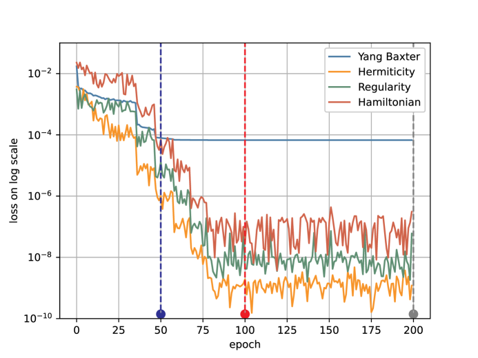
Figure 2: The evolution of training losses for the XYZ model, shown on the log scale. The losses tend to fall in a step-wise manner, which corresponds approximately to the learning rate schedule the network is trained with.

Figure 3 plots the R-matrix component ratios with respect to $R_{12}$ in terms of the spectral parameter, and compares them with the corresponding analytic functions for a generic choice of deformation parameters $\eta=\frac{\pi}{3}$ and $m=0.6$. Letting $m=0$, we recover the XXZ models for generic values of $\eta$.

[] []

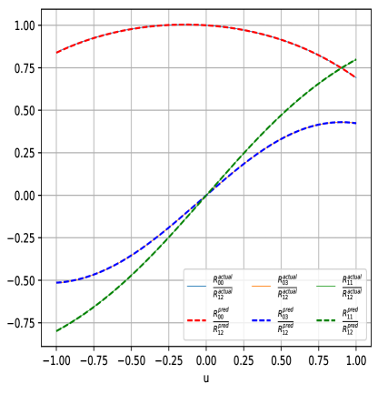
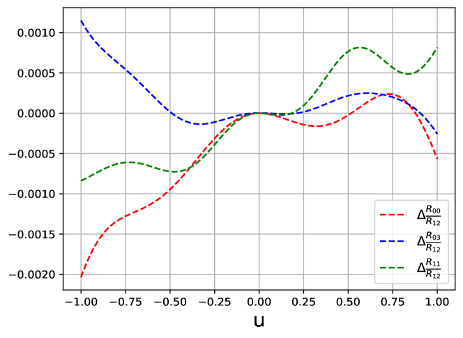
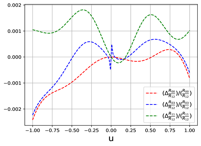
Figure 3: (a) XYZ R-matrix as ratios with respect to the (12) component for $\eta=\pi/3,m=0.6$, (b) Relative and absolute errors for R-matrix.

4.1.2 Two-dimensional classification

Here, we lift the hermiticity constraint on the Hamiltonian, thus allowing for more generic integrable models. As we shall see below, the neural network successfully learns all the 14 classes[58] of difference-form integrable (not necessarily Hermitian) spin chain models with 2-dimensional space at each site. The R-matrices corresponding to each of these classes are written down explicitly in appendix A. Towards the end of this sub-section, we also present results for learning solutions in generic gauge obtained by similarity transformation of integrable Hamiltonians from the aforementioned 14 classes. We shall discuss the results in two parts: XYZ type models, and non-XYZ type models.

The first set of Hamiltonians under consideration are generalisations of the XYZ model (discussed in the previous sub-section), with at most 8 non-zero elements in its Hamiltonian density

$$H_{8-\text{vertex}}=\begin{pmatrix}a_{1}&0&0&d_{1}\\ 0&b_{1}&c_{1}&0\\ 0&c_{2}&b_{2}&0\\ d_{2}&0&0&a_{2}\end{pmatrix}$$ (4.5)

where the coefficients can take generic complex values. The XYZ model corresponds to the subset with $a_{1}=a_{2},b_{1}=b_{2},c_{1}=c_{2},d_{1}=d_{2}$. As discussed in section 2.1, these models can be further sub-divided into four, six, seven and eight vertex models. On the other hand, there are 6 distinct classes of non-XYZ type solutions. Here we will discuss the training results for one example each from the XYZ and non-XYZ type models, since the training behaviour is similar within these two types. Rest of the models will be presented in Appendix A. Figure 4 plots the R-matrix components as ratios with respect to $R_{00}$ for a generic 6-vertex model with $d_{1}=d_{2}=0$, and $a_{1}=a_{2}$. The figure also includes the absolute and relative errors with respect to the corresponding analytic R-matrix (see equation (A.2)).

[] []

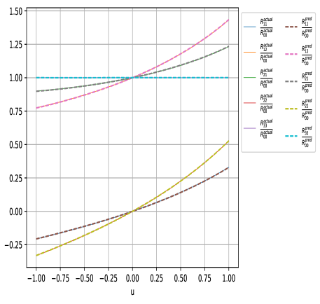
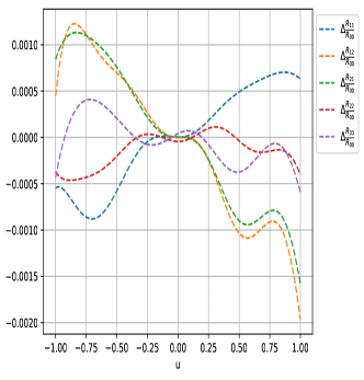
Figure 4: (a) Predicted vs actual R-matrix component ratio w.r.t. $R_{00}$ for XXZ-type model with $a_{1}=a_{2}=0.3,b_{1}=0.45,b_{2}=0.6,c_{1}=0.4,c_{2}=0.25$, (b) Absolute error between predicted and actual R-matrix component ratios

From the non-XYZ classes, we will focus on the following 5-vertex Hamiltonians

$$H_{class-1}=\begin{pmatrix}0&a_{1}&a_{2}&0\\ 0&a_{5}&0&a_{3}\\ 0&0&-a_{5}&a_{4}\\ 0&0&0&0\end{pmatrix}$$ (4.6)

For integrability, we require the additional condition

$$a_{1}a_{3}=a_{2}a_{4}\,.$$ (4.7)

Training the Hamiltonian constraint (3.13) for generic values $a_{1}=0.5,a_{2}=0.3,a_{3}=0.9,a_{4}=1.5,a_{5}=0.4$ satisfying the above integrability condition, we get over $0.1\%$ accuracy for training over $\sim$100 epochs. Figure 5 plots the trained R-matrix components and absolute errors with respect to the analytic R-matrices in equation (A.20), for the above choice of target Hamiltonian.

[] []

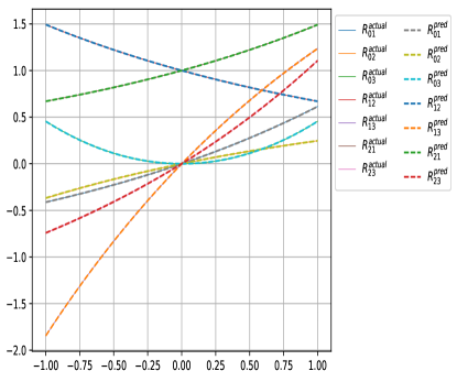
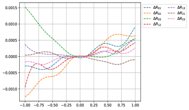
Figure 5: (a) Predicted vs actual R-matrix components for the Hamiltonian of class-1, with coefficients $a_{1}=.5,\,a_{2}=.3,\,a_{3}=.9,\,a_{4}=1.5,\,a_{5}=.4$. Note here the R-matrices are automatically normalised since $R_{00}$ was fixed to the constant value of 1, (b) Absolute error between predicted and actual R-matrix components

We have also surveyed more general solutions beyond the representative solutions of the 14 classes a la [58], by changing the gauge of the R-matrix as well as the corresponding Hamiltonian. As noted earlier in section 2, we can act with a $2\times 2$ similarity matrix $\Omega$ on the R-matrix :

$$R(u)\rightarrow R^{\Omega}(u)=(\Omega\otimes\Omega)R(u)(\Omega^{-1}\times\Omega^{-1})$$ (4.8)

$$H\rightarrow H^{\Omega}=(\Omega\otimes\Omega)H(\Omega^{-1}\times\Omega^{-1})$$ (4.9)

If $R(u)$ satisfies Yang-Baxter equation, so does $R^{\Omega}(u)$. A generic similarity matrix $\Omega$

$$\Omega=\begin{pmatrix}v_{11}&v_{12}\\ v_{21}&v_{22}\end{pmatrix}$$ (4.10)

with non-zero off-diagonal entries $v_{12},v_{21}\neq 0$, results in conjugated R-matrices and Hamiltonians with all 16 non-zero entries. We trained 16-vertex Hamiltonians resulting from XYZ model in the general gauge and recovered the corresponding R-matrix with a relative error of order $\mathcal{O}(0.1\%)$. Generic XYZ type models, as well as non-XYZ type models gave similar results for different gauges. Figure 6 plots the learnt R-matrix components for XXZ model with $\eta=\frac{\pi}{3}$ conjugated by the matrix $\Omega$ =$\begin{pmatrix}0.4&0.5\\ -1.2&1\end{pmatrix}$. For comparison with analytic formulae, we normalised our results by taking ratios with respect to a fixed component $R_{00}$, i.e. we plot $\frac{R_{ij}}{R_{00}}$. As a result of starting from the XXZ model, the R-matrix $R_{XXZt}$ in the general gauge has following highly symmetric form

$$R_{XXZg}=\begin{pmatrix}R_{00}&R_{01}&R_{01}&R_{03}\\ R_{10}&R_{11}&R_{12}&-R_{01}\\ R_{10}&R_{12}&R_{11}&-R_{01}\\ R_{30}&-R_{10}&-R_{10}&R_{00}\end{pmatrix}$$ (4.11)

Thus we only plot the entries $R_{00},R_{01},R_{03},R_{10},R_{11},R_{12},R_{30}$. Since there exists overall normalisation ambiguity, we should only compare ratio of R-matrix entries with the analytic solution written in the same gauge.

[] []

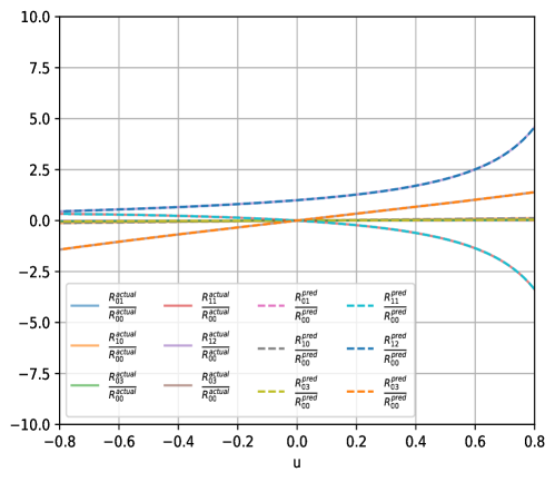
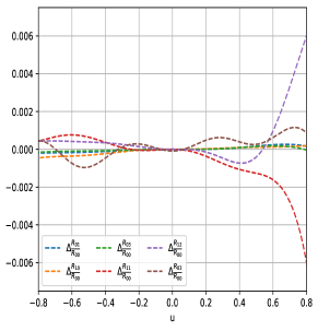
Figure 6: (a) Predicted R-matrix component ratios w.r.t. $R_{00}$, for conjugated XXZ model with $\eta=\frac{\pi}{3}$ and similarity matrix $\Omega=\small\begin{pmatrix}0.4&0.5\\ -1.2&1\end{pmatrix}$, (b) Absolute error between predicted and actual R-matrix ratios

Next we discuss the difference in the training of integrable vs non-integrable models with our neural network. We will focus on two representative examples : 6-vertex model with Hamiltonian $H_{6v,1}$, and class 4 models with Hamiltonian $H_{class-4}$. Similar results hold across all the 14 classes.

For 6-vertex models with Hamiltonians following equation (4.5) with $d_{1}=d_{2}=0$, generic values of the coefficients $a_{i},b_{i},c_{i},d_{i}$ for $i=1,2$ leads to non-integrable models, unless

$$a_{1}=a_{2}\,,\quad a_{1}+a_{2}=b_{1}+b_{2}\,.$$ (4.12)

These are the models with Hamiltonian $H_{6v,1}$, $H_{6v,2}$ in appendix A. Figure 7(a) compares the training for a generic Hamiltonian with coefficients satisfying none of the above conditions against the training for $H_{6v,1}$-type model. We see that while the Hamiltonian constraint (3.13) saturates to similarly low values in both cases, the Yang-Baxter loss saturates at approximately one order of magnitude higher.

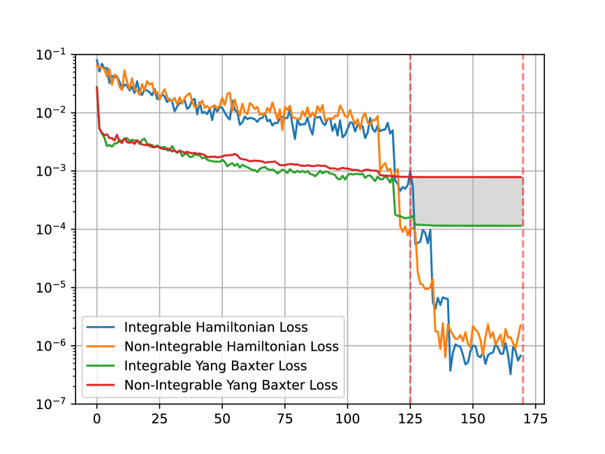
(a) Hamiltonian $H_{6v,1}$ vs non-integrable.

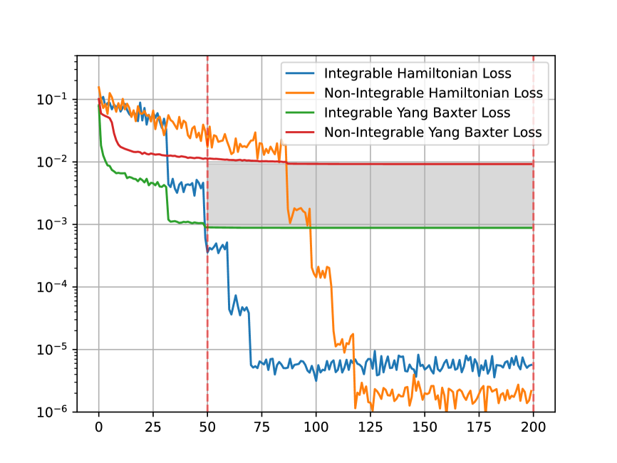
(b) Hamiltonian $H_{\mathrm{class}-4}$ vs non-integrable.

Figure 7: Comparing the training history of the Type XYZ and non-XYZ models against corresponding non-integrable Hamiltonians. There is approximately an order of magnitude difference between the Yang-Baxter losses for the integrable case vs the non-integrable case after the training saturates, indicated by the gray region in the graph. The step-wise drops in the loss functions approximately correspond to the learning rate schedule. The presented Hamiltonians are the same as on Fig.8 and Fig.9

Similar behavior holds for the non-XYZ type models as well. The training for a generic class-4 Hamiltonian with coefficients $a_{1}=0.5,a_{2}=0.3,a_{3}=0.4,a_{4}=0.9$ (see Equation A.19) and a non-integrable deformation is shown in Figure 7(b).

One can further discriminate between integrable and non-integrable models by checking the point-wise values of the Yang-Baxter losses in the two cases. Let us define the metric

$$\tilde{\mathcal{L}}=\frac{||\mathcal{R}_{12}(u-v)\mathcal{R}_{13}(u)\mathcal{R}_{23}(v)-\mathcal{R}_{23}(v)\mathcal{R}_{13}(u)\mathcal{R}_{12}(u-v)||}{||\mathcal{R}_{12}(u-v)\mathcal{R}_{13}(u)\mathcal{R}_{23}(v)||}\,,$$ (4.13)

which measures the relative error in the approximate solution of the Yang-Baxter equation. This metric is evaluated for the trained R-matrix for both integrable and non-integrable models in Figure 8 (for $H_{6v,1}$ model), and Figure 9 (for $H_{class-4}$ model). We see that the normalized error can be up to two orders of magnitude larger for the non-integrable case. Note that irrespective of the choice of Hamiltonian, there are two lines along $u=v$ and $v=0$ on which the Yang-Baxter equation is trivially satisfied, due to regularity. This metric also can detect anomalous situations when the learned solution once satisfied the Hamiltonian constraint at $u=0$ quickly evolves to a true solution of Yang-Baxter equation producing relatively small YB loss (3.7). In this case we will see the big spike in (4.13) around zero which will indicate the fakeness of the found solution.

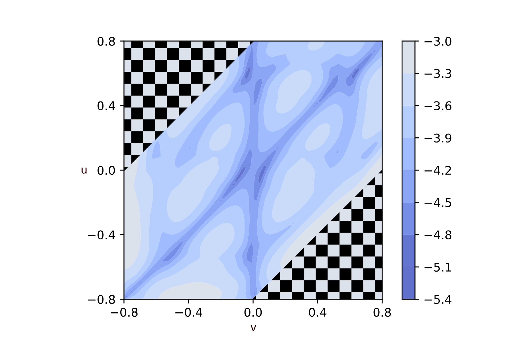
(a) $H_{6v,1}$

(b) $H_{6v,1}$ deformation

Figure 8: (a) The normalized Yang-Baxter error (4.13) plotted in the logarithmic scale at the end of training for the Hamiltonian $H_{6v,1}$ with $a_{1}=0.3,a_{2}=0.3,b_{1}=0.45,b_{2}=0.6,c_{1}=0.4,c_{2}=0.25$, and (b) its non-integrable deformation with $a_{1}=-1.3,a_{2}=1.3$ and other parameters kept constant. In order to keep all three arguments appearing in YB equation inside the same inteval $|u|,|v|,|u-v|<0.8$ we cut out the area $|u-v|>0.8$ with chess-pattern triangles.

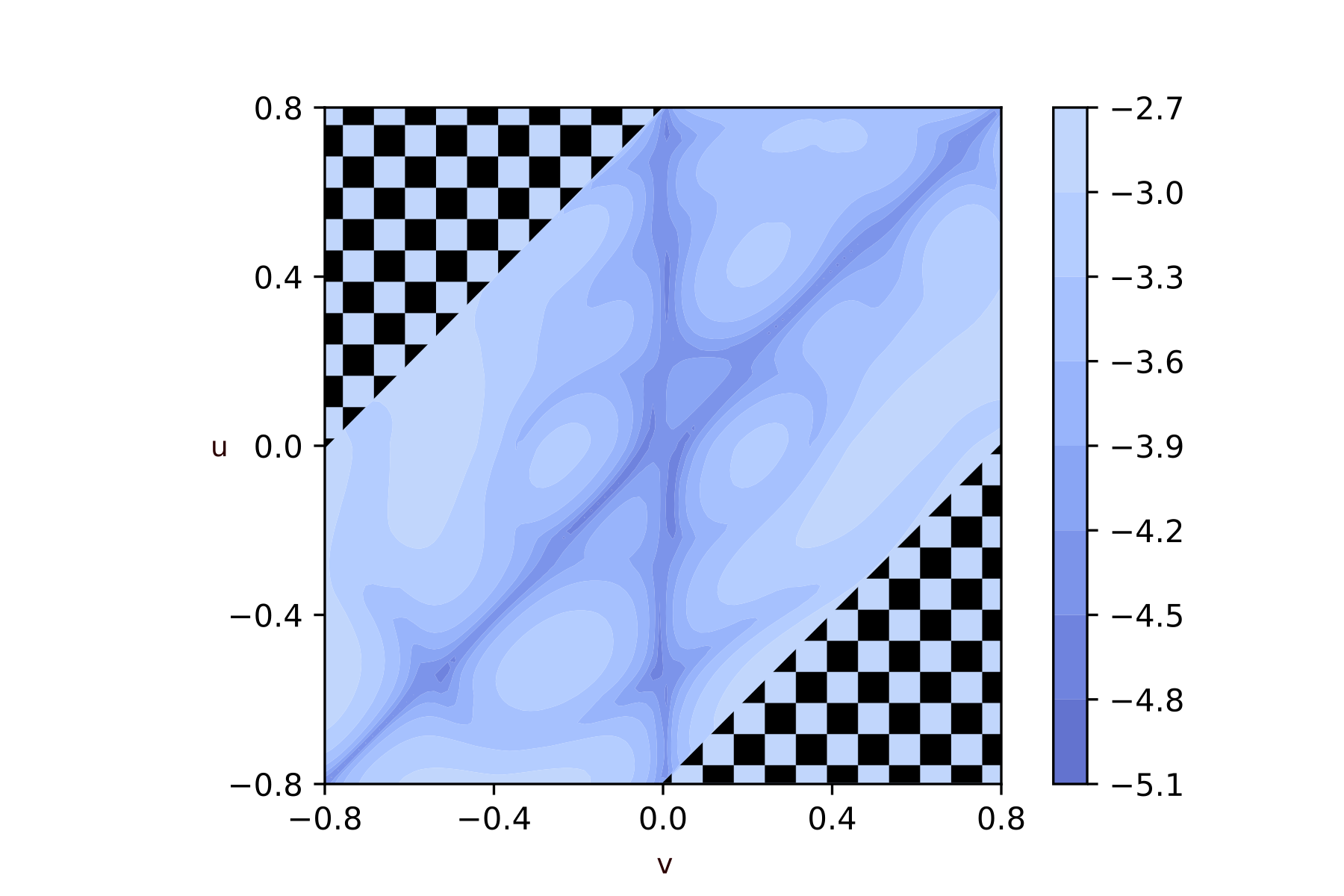
(a) $H_{\mathrm{class}-4}$

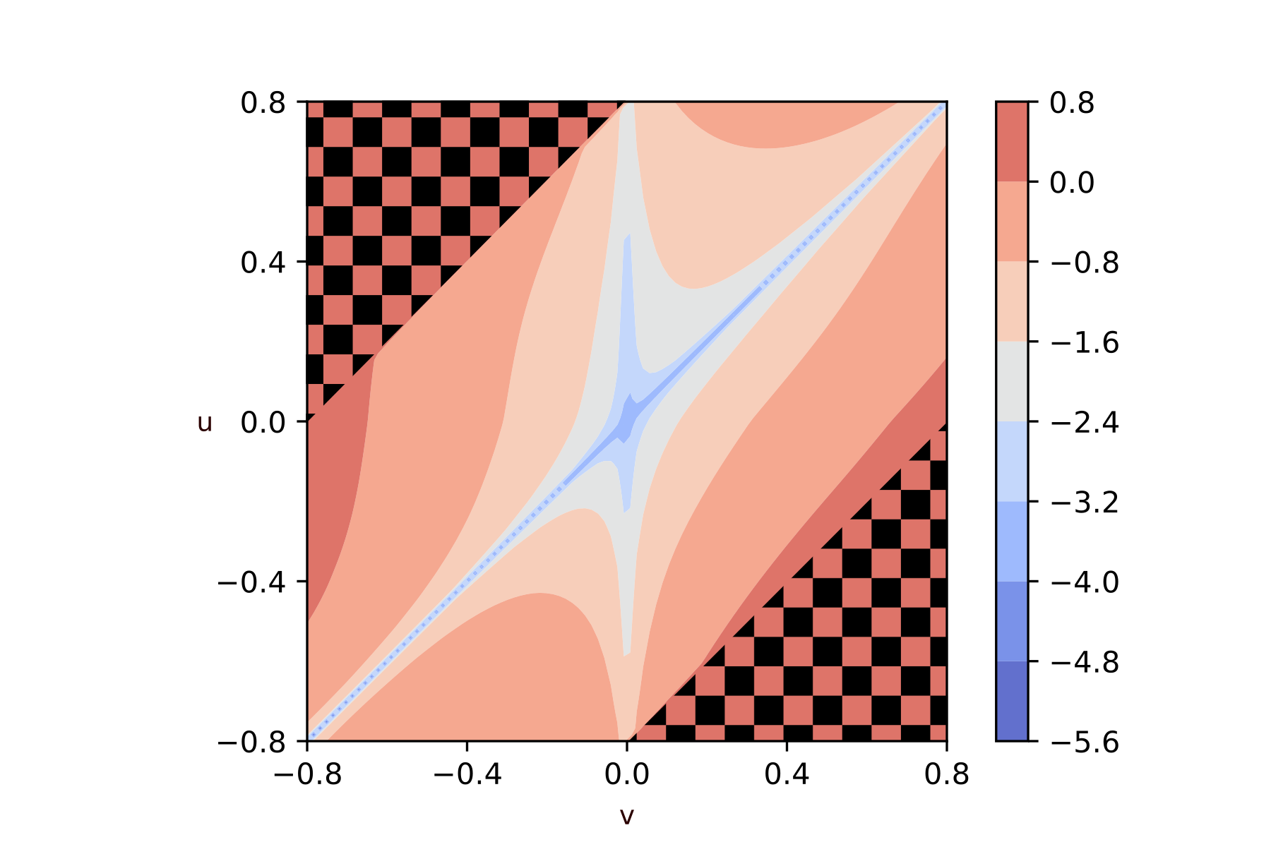
(b) $H_{\mathrm{class}-4}$ deformation

Figure 9: (a) The normalized Yang-Baxter error (4.13) plotted in the logarithmic scale at the end of training for the Hamiltonian $H_{class-4}$ from (A.19), with $a_{1}=0.5,a_{2}=0.3,a_{3}=0.4,a_{4}=0.9$, (b) Non-integrable deformation with same Hamiltonian parameters as in the integrable case, except for $H_{13}=-0.9$.

The above consideration shows that one can define the metrics which together indicate the closeness of the given system to the integrable Hamiltonian. However, the final conclusion in the binary form of ``integrable/nonintegrable" regarding the given spin chain can be made only asymptotically, namely increasing the number of neurons, density of points and training time one can get the normalized YB loss (4.13) uniformly decreasing to zero for integrable Hamiltonians while for nonintegrable case it will be bounded from below by some positive value. Also let's stress that such problem is specific for the solver mode once we stick to a given Hamiltonian, while in the case of relaxed Hamiltonian restrictions as we will see in the next section, the neural network moves to the true solution of the Yang-Baxter equation.

4.2 Explorer: new from existing

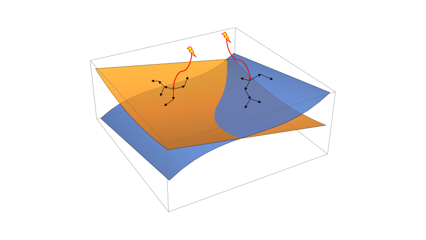
Figure 10: Visualizing the Explorer scheme. We start with random initializations, marked by lightning symbols, and perform solver learning represented by red curve arrows. Once we reach an submanifold of integrable Hamiltonians, we explore it using repulsion to identify new integrable models.

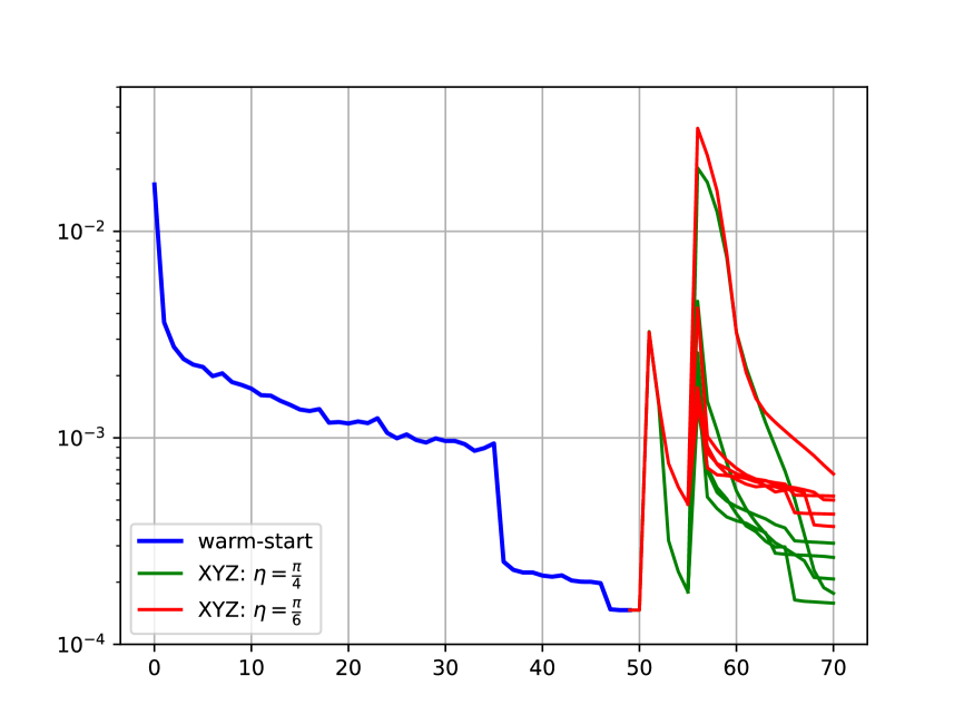
(a) Evolution of Yang-Baxter Loss

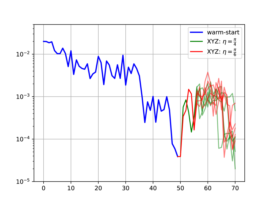
(b) Evolution of Hamiltonian Loss

Figure 11: The convergence to XYZ models from XXZ models trained with different parameters. XXZ was trained for 50 epochs at $\eta=\frac{\pi}{3}$ and $m=0$. Then, it was trained for 5 more epochs at $\eta=\frac{\pi}{4}$ and $\eta=\frac{\pi}{6}$, still with $m=0$. After that, 5 non-zero values of $m$ were used for each XXZ model, and we trained for another 15 epochs. Loss spikes occurred when the target hamiltonian values were reset. The final training was run in parallel for convenience, but it can be run sequentially.

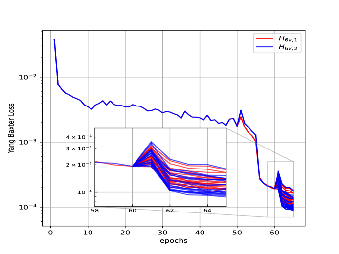
Figure 12: Time evolution of the Yang Baxter loss as the neural network explores the space of integrable Hamiltonians of 6-vertex models $H_{6v1,6v2}$ by repulsion. The loss evolves together until the $50^{th}$ epoch after which it fragments slightly as the training converges to the two warm-start points on the 60th epoch. For the remaining epochs the losses fragment completely as the neural network seeks out different new Hamiltonians and is terminated when the loss reaches the neighborhood of $1\times 10^{-4}$.

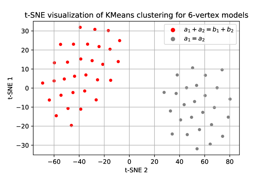
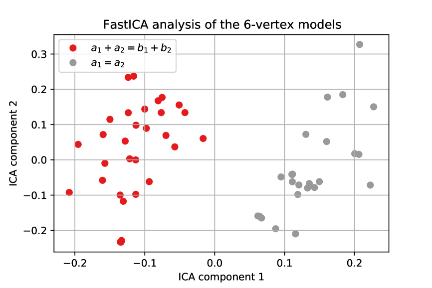
Figure 13: Clustering of Hamiltonians from the 2 classes of gauge-inequivalent 6-vertex models obtained by Explorer using repulsion from solution at intersection of both classes.

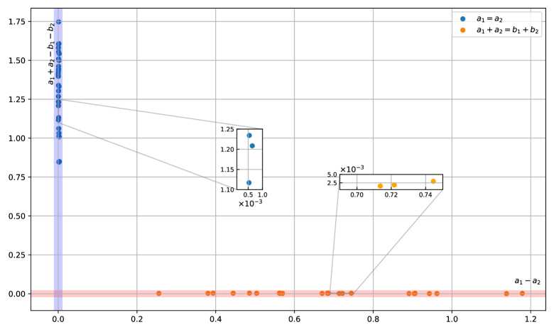
Figure 14: The 6-vertex models learnt by exploration. The graph visualizes the obtained Hamiltonians by plotting their values along the $a_{1}+a_{2}-b_{1}-b_{2}$ and the $a_{1}-a_{2}$ axes. The models $H_{6v,1}$ lie along the $y$-axis and the models $H_{6v,2}$ along the $x$-axis with an error margin of order $10^{-3}$ as shown in the telescoped inset plots.

In this section we will present two kinds of experiments that illustrate how the neural network presented above can be used to scan the landscape of two-dimensional spin-chains for integrable models. The training schedule adopted in this section is visualized in Figure 10 and relies essentially on two new ingredients which distinguish it from the previous solver framework. These are warm-start and repulsion. We will illustrate each by an example. In the first case we shall simply use warm-start, and in the second, we shall combine warm-start with repulsion. Finally, we shall use unsupervised learning methods such as t-SNE and Independent Component Analysis to identify distinct classes of Hamiltonians within the set of integrable models thus discovered. Collectively, these strategies make up our explorer framework.

The first key new ingredient is a warm-start initialization. As mentioned previously, the standard solver framework of the previous section uses He initialization [64] to instantiate the weights and biases of the neural network. In warm-start initialization, we use the knowledge of integrable systems previously discovered by the neural network to find new systems in its vicinity. The idea, at least intuitively, is that it should be possible to find new integrable systems more efficiently than with the random initialization by exploring the vicinity in weight-space of previously determined solutions using an iterative procedure such as gradient-based optimization. On doing so, we find a significant acceleration in training convergence, with new solutions being discovered typically in about 5 epochs of training after warm-start initialization. For definiteness, we consider the hermitian XYZ model discussed earlier in Section 4.1.1. This has a two-parameter family of solutions, corresponding to independent choices for the parameters $\eta$ and $m$ of the Jacobi elliptic function, as seen from Equation (4.4). The XXZ model is embedded into this space as the $m=0$ subspace of solutions.

We now describe how the above strategy can be used to quickly generate the cluster of XYZ R-matrices starting from a particular one which we choose from XXZ subclass. We begin with pre-training our neural network using the solver mode of the previous section, but with the learning rate of the Adam optimizer set to $10^{-3}$. The pre-training is stopped when all losses saturate below $\mathcal{O}\left(10^{-3}\right)$, which typically requires about 50 epochs of training. We carried out this pre-training setting arbitrary reference values of $\eta$, but with $m$ fixed to zero. The results shown here correspond to $\eta=\frac{\pi}{4}$. The weights thus obtained correspond to our warm-start values. Then we shift the target Hamiltonian values to correspond to $\eta\rightarrow\eta+\delta\eta$, where $\delta\eta$ are randomly chosen $\mathcal{O}\left(10^{-1}\right)$ numbers, and $m$ can take on non-zero values as well. We then retrain the model with a smaller learning rate, $10^{-4}$ for a few epochs until all loss terms fall to $\mathcal{O}\left(10^{-4}\right)$, which typically takes about 5 epochs, upon which we update the target Hamiltonian by updating $\eta$ and $m$ and continue training. This strategy generates about 10 XYZ models within the same time-scale (i.e. about 100 to 200 epochs of training) as we earlier needed for a single model. For best results, while we randomly update $\eta$, we systematically anneal the modular parameter $m$ to upwards of zero. A sample of this training is visualized in Figure 11(b).

Our next key new ingredient for the Explorer mode is repulsion, which is added to the previous strategy of warm-start initialization. In principle, it should allow us to rediscover all 14 classes of integrable spin chains. However, for sake of simplicity, we will illustrate it now with a toy-model example and return to the general analysis later [71]. Namely, we consider the class of 6-vertex Hamiltonians with unrestricted $a_{1}$ and $a_{2}$. It includes both integrable 6-vertex classes $H_{6v,1},H_{6v,2}$ (A.2, A.4) as well as nonintegrable models. In order to mimic the general situation when all integrable classes intersect at zero, we begin by pre-training the neural network to a Hamiltonian belonging to the intersection of the classes $H_{6v,1}$ and $H_{6v,2}$, i.e. whose matrix element satisfy the constraints $a_{1}=a_{2}$ and $a_{1}+a_{2}=b_{1}+b_{2}$ simultaneously. The results mentioned in this paper correspond to setting

$$a_{1}=a_{2}=\frac{b_{1}+b_{2}}{2}\,;\qquad b_{1}=0.6,\,b_{2}=0.8,\,c_{1}=0.5,\,c_{2}=0.9\,.$$ (4.14)

Having arrived at this model, we would like to navigate to neighboring models not by specifying target values of the Hamiltonian, but by scanning the neighborhood of the current model. To do so, we employ a two step strategy. First, we navigate to two new 6-vertex integrable Hamiltonians by random scanning the vicinity of the current model without giving specific target values. We shall use these new models as our warm-start points. From each of them, we navigate away by using the $repulsion$ loss term (3.17) for 1 epoch, followed by training for another 5 epochs. Note in this step, we still train within the restricted class of 6-vertex models by fixing the corresponding entries of the R-matrix to zero. We repeat this schedule 25 times starting from either of the saved models. This way, we generate fifty 6-vertex integrable Hamiltonians with over 1% accuracy. The training curve displaying how the Yang-Baxter loss evolves is shown in Figure 12.

The learnt models are classified into two classes using clusterisation methods as shown in Figure 13. Figure 14 plots the trained models in terms of coordinates defined by the integrability conditions of the Hamiltonians $H_{6v,1},H_{6v,2}$. Models lying near the two axes were classified correctly into the two classes in Figure 13 with $100\%$ accuracy.

5 Conclusions and Future directions

In this paper we constructed a neural network for solving the Yang-Baxter equation (2.3) in various contexts. Firstly, it can learn the R-matrix corresponding to a given integrable Hamiltonian or search for an integrable spin chain and the corresponding R-matrix from a certain class specified by imposed symmetries or other restrictions. We refer to this as the solver mode. Next, in the explorer mode, it can search for new integrable models by scanning the space of Hamiltonians.

We demonstrated the use of our neural network on two-dimensional spin chains of difference form. In the solver mode, the network successfully learns all fourteen distinct classes of R-matrices identified in [58] to accuracies of the order of $0.01-0.1\%$. We demonstrated the work of the Explorer mode, restricting the search to the space of spin chains containing both classes of 6-vertex models as well as nonintegrable Hamiltonians. Starting from the hamiltonian at the intersection of two classes , Explorer found 50 integrable Hamiltonians which after clusterisation clearly fall into two families corresponding to two integrable classes of 6-vertex model. Working in the explorer mode, we find that warm-starting our training from the vicinity of a previously learnt integrable model greatly speeds up convergence, allowing us to identify typically about 50 new integrable models in the same time that random initialization takes to converge to a single model.

The main focus of this paper was creating the neural network architecture and demonstrating its robustness in various solution generating frameworks using known integrable models as a testing ground. However, we expect that this program can be extended to various scenarios such as the exploration and classification of the space of integrable Hamiltonians in dimensions greater than two. This would be of great interest since the general classification of models is currently limited to two dimensions. Our experiments with exploration and clustering are a promising starting point in this regard. In our setup the strategy is quite straightforward [71]. Because all integrable families of Hamiltonians can be multiplied by arbitrary scalar, we should only scan the Hamiltonians on the unit sphere which is compact. Scanning over sufficiently dense set of points on the sphere will allow us to identify integrable Hamiltonians from various classes. Then we can use the Explorer to reconstruct the whole corresponding families and perform clusterisation in order to identify them. On another footing, it would also be interesting to extend our study to R-matrices of non-difference form as these are particularly relevant to the AdS/CFT correspondence [72, 73, 74, 75].

While our network learns a numerical approximation to the R-matrix, it can also be useful for the reconstruction of analytical solutions using symbolic regression [29, 76]. Alternately, one may try to use the learnt numerical solution for the reconstruction of the symmetry algebra such as the Yangian and then arrive at the analytical solution. Remarkably, machine learning is already proving helpful in the analysis of symmetry in physical systems. In particular, one may verify the presence of a conjectured symmetry or even automate its search using machine learning [19, 43, 44, 45, 46, 47, 77]. It would be very interesting to explicate the interplay of our program in this broader line of investigation.

In addition, the flexibility of our approach would also allow us to implement various additional symmetries or other restrictions, both at the level of the R-matrix and the Hamiltonian. It would therefore be very interesting to develop an `R-matrix bootstrap' in the spirit of the two-dimensional S-matrix bootstrap and analyze the interplay between various symmetries. For example, all 14 families of R-matrices considered in this paper satisfy the condition of braided unitarity (2.12) and it would be interesting to rediscover them from the use of braided unitarity and other symmetries without imposing the Yang-Baxter condition, similar to how integrable two-dimensional S-matrices have been identified in the S-matrix Bootstrap approach [51, 53, 78].

With mild modifications, we can adapt our architecture to the analysis of Yang-Baxter equation for the integrable S-matrices in two dimensions. The only new feature to implement is the analytic structure in the s-plane. It can be naturally realized with the use of holomorphic networks.

Learning solutions for different classes with the same architecture, we noticed that the number of epochs needed to reach the same precision varies for different classes while being roughly the same for the Hamiltonians from the same classes. Thus, it would be very tempting to use the training of losses to define the complexity of spin chains. Ideally, we should be able to go beyond the class of integrable models and see that they sit at the minima of complexity, matching common beliefs that the integrable models are the ``simplest" ones.

Appendix A Classes of 2D integrable spin chains of difference form

In this appendix, we list the 14 gauge-inequivalent integrable Hamiltonians of difference form and the corresponding R-matrices. Amongst the XYZ type models, the simplest solution is a diagonal 4-vertex model with Hamiltonians and R-matrices as follows:

$$H_{4v}=\begin{pmatrix}a_{1}&0&0&0\\ 0&b_{1}&0&0\\ 0&0&b_{2}&0\\ 0&0&0&a_{2}\end{pmatrix}\,\leftrightarrow\quad R_{4v}(u)=\begin{pmatrix}e^{a_{1}u}&0&0&0\\ 0&0&e^{b_{2}u}&0\\ 0&e^{b_{1}u}&0&0\\ 0&0&0&e^{a_{2}u}\end{pmatrix}$$ (A.1)

Figure 15 plots the training curve for R-matrix components as ratios with respect to (00) component, against the analytic functions for parameters $a_{1}=0.9,b_{1}=0.4,b_{2}=0.6,a_{2}=0.75$.

[] []

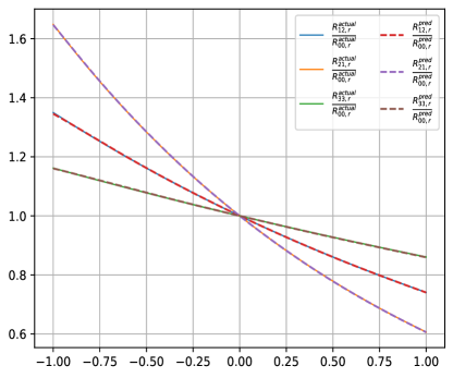
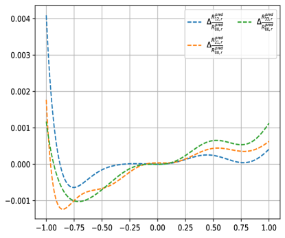
Figure 15: (a) 4-vertex model, with $H_{2}$ parameters $a_{1}=0.9,\,b_{1}=0.4,\,b_{2}=0.6,\,a_{2}=0.75$, (b) errors

In 6-vertex models, we have two distinct classes depending on whether the Hamiltonian entries $H^{00}$ and $H^{33}$ are equal or not. In the first case, the R-matrix $R_{6v,1}(u)$ and its associated Hamiltonian $H_{6v,1}$ are given by

$$H_{6v,1}=\begin{pmatrix}a_{1}&0&0&0\\ 0&b_{1}&c_{1}&0\\ 0&c_{2}&b_{2}&0\\ 0&0&0&a_{1}\end{pmatrix}\,\leftrightarrow\quad R_{6v,1}(u)=\begin{pmatrix}R_{6v,1}^{00}(u)&0&0&0\\ 0&R_{6v,1}^{11}(u)&R_{6v,1}^{12}(u)&0\\ 0&R_{6v,1}^{21}(u)&R_{6v,1}^{22}(u)&0\\ 0&0&0&R_{6v,1}^{33}(u)\end{pmatrix}$$ (A.2)

where

$$\begin{split}R_{6v,1}^{00}(u)&=R_{6v,1}^{33}(u)=e^{(b_{1}+b_{2})u/2}(\cosh{(\omega u)}+\frac{2a_{1}-b_{1}-b_{2}}{2\omega}\sinh{(\omega u)})\\ R_{6v,1}^{11}(u)&=\frac{c_{2}}{\omega}e^{(b_{1}+b_{2})u/2}\sinh{(\omega u)}\\ R_{6v,1}^{12}(u)&=e^{b_{2}u}\\ R_{6v,1}^{21}(u)&=e^{b_{1}u}\\ R_{6v,1}^{22}(u)&=\frac{c_{1}}{\omega}e^{(b_{1}+b_{2})u/2}\sinh{(\omega u)}\,,\qquad\omega=\frac{\sqrt{(2a_{1}-b_{1}-b_{2})^{2}-4c_{1}c_{2}}}{2}\end{split}$$ (A.3)

Figure 4 gives a representative training vs actual plot for this class.

For the case $H^{00}\neq H^{33}$, the R-matrix $R_{6v,2}(u)$ is given by

$$H_{6v,2}=\begin{pmatrix}a_{1}&0&0&0\\ 0&b_{1}&c_{1}&0\\ 0&c_{2}&b_{2}&0\\ 0&0&0&a_{2}\end{pmatrix}\,\leftrightarrow\quad R_{6v,2}(u)=\begin{pmatrix}R_{6v,2}^{00}(u)&0&0&0\\ 0&R_{6v,2}^{11}(u)&R_{6v,2}^{12}(u)&0\\ 0&R_{6v,2}^{21}(u)&R_{6v,2}^{22}(u)&0\\ 0&0&0&R_{6v,2}^{33}(u)\end{pmatrix}$$ (A.4)

where $a_{2}=b_{1}+b_{2}-a_{1}$ and

$$\begin{split}R_{6v,2}^{00}(u)&=e^{(a_{1}+a_{2})u/2}(\cosh{(\omega u)}+\frac{a_{1}-a_{2}}{2\omega}\sinh{(\omega u)})\\ R_{6v,2}^{11}(u)&=\frac{c_{2}}{\omega}e^{(a_{1}+a_{2})u/2}\sinh{(\omega u)}\\ R_{6v,2}^{12}(u)&=e^{b_{2}u}\\ R_{6v,2}^{21}(u)&=e^{b_{1}u}\\ R_{6v,2}^{22}(u)&=\frac{c_{1}}{\omega}e^{(a_{1}+a_{2})u/2}\sinh{(\omega u)}\\ R_{6v,2}^{33}(u)&=e^{(a_{1}+a_{2})u/2}(\cosh{(\omega u)}-\frac{a_{1}-a_{2}}{2\omega}\sinh{(\omega u)})\,,\qquad\omega=\frac{\sqrt{(a_{1}-a_{2})^{2}-4c_{1}c_{2}}}{2}\end{split}$$ (A.5)

Figure 16 gives a representative training vs actual plot for Hamiltonian parameters $a_{1}=1.,a_{2}=0.2,b_{1}=0.45,b_{2}=0.75,c_{1}=0.4,c_{2}=0.6$.

[] []

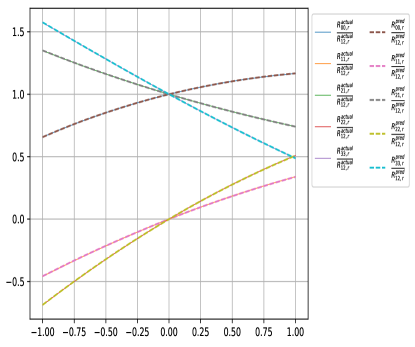
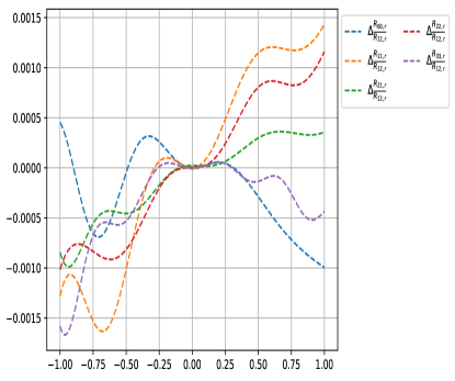
Figure 16: (a) 6-vertex model with Hamiltonian of type $H_{6v,2}$, with parameters $a_{1}=1,a_{2}=0.2,b_{1}=0.45,b_{2}=0.75,c_{1}=0.4,c_{2}=0.6$, (b)errors

Next we have the 7-vertex models, which consists of two classes of solution distinguished by the Hamiltonian entries $H^{00}$, $H^{33}$ being equal or not. In the first case, we have

$$H_{7v,1}=\begin{pmatrix}a_{1}&0&0&d_{1}\\ 0&a_{1}+b_{1}&c_{1}&0\\ 0&-c_{1}&a_{1}-b_{1}&0\\ 0&0&0&a_{1}\end{pmatrix}\,\leftrightarrow\quad R_{7v,1}(u)=\begin{pmatrix}R_{7v,1}^{00}(u)&0&0&R_{7v,1}^{03}(u)\\ 0&R_{7v,1}^{11}(u)&R_{7v,1}^{12}(u)&0\\ 0&R_{7v,1}^{21}(u)&R_{7v,1}^{22}(u)&0\\ 0&0&0&R_{7v,1}^{33}(u)\end{pmatrix}$$ (A.6)

where

$$\begin{split}R_{7v,1}^{00}(u)&=R_{7v,1}^{33}(u)=e^{a_{1}u}\cosh{(c_{1}u)}\\ R_{7v,1}^{11}(u)&=-R_{7v,1}^{22}(u)=e^{a_{1}u}\sinh{(c_{1}u)}\\ R_{7v,1}^{12}(u)&=e^{(a_{1}-b_{1})u}\\ R_{7v,1}^{21}(u)&=e^{(a_{1}+b_{1})u}\\ R_{7v,1}^{03}(u)&=-\frac{d_{1}}{2b_{1}}(e^{(a_{1}-b_{1})u}-e^{(a_{1}+b_{1})u})\end{split}$$ (A.7)

Figure 17 plots the predicted R-matrix components as ratios with respect to the $(12)$ component against the above analytic results, and their differences for a generic choice of parameters $a_{1}=1,b_{1}=0.45,c_{1}=0.6,d_{1}=0.75$.

[] []

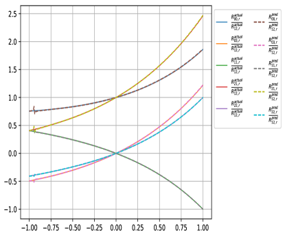
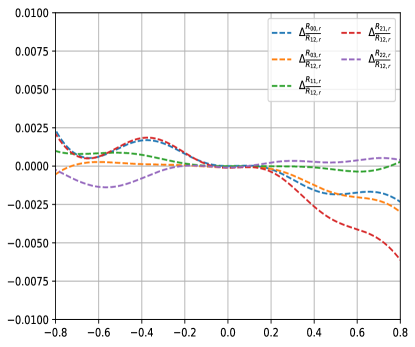
Figure 17: (a) 7-vertex model with Hamiltonian of type $H_{7v,1}$, with parameters $a_{1}=1,b_{1}=0.45,c_{1}=0.6,d_{1}=0.75$, (b)errors

In the second case for $H^{00}\neq H^{33}$, we have

$$H_{7v,2}=\begin{pmatrix}a_{1}&0&0&d_{1}\\ 0&a_{1}-c_{2}&c_{1}&0\\ 0&c_{2}&a_{1}-c_{1}&0\\ 0&0&0&a_{2}\end{pmatrix}\,\leftrightarrow\quad R_{7v,2}(u)=\begin{pmatrix}R_{7v,2}^{00}(u)&0&0&R_{7v,1}^{03}(u)\\ 0&R_{7v,2}^{11}(u)&R_{7v,1}^{12}(u)&0\\ 0&R_{7v,2}^{21}(u)&R_{7v,1}^{22}(u)&0\\ 0&0&0&R_{7v,1}^{33}(u)\end{pmatrix}$$ (A.8)

where $a_{2}=a_{1}-c_{1}-c_{2}$ and

$$\begin{split}R_{7v,2}^{00}(u)&=\frac{e^{(a_{1}-\frac{c_{1}+c_{2}}{2})u}}{c_{1}-c_{2}}((c_{1}-c_{2})\cosh{(\frac{c_{1}-c_{2}}{2}u)}+(c_{1}+c_{2})\sinh{(\frac{c_{1}-c_{2}}{2}u)})\\ R_{7v,2}^{11}(u)&=\frac{2c_{2}}{c_{1}-c_{2}}e^{(a_{1}-\frac{c_{1}+c_{2}}{2})u}\sinh{(\frac{c_{1}-c_{2}}{2}u)}\\ R_{7v,2}^{22}(u)&=\frac{2c_{1}}{c_{1}-c_{2}}e^{(a_{1}-\frac{c_{1}+c_{2}}{2})u}\sinh{(\frac{c_{1}-c_{2}}{2}u)}\\ R_{7v,2}^{12}(u)&=e^{(a_{1}-c_{1})u}\\ R_{7v,2}^{21}(u)&=e^{(a_{1}+c_{2})u}\\ R_{7v,2}^{03}(u)&=\frac{2d_{1}}{c_{1}-c_{2}}e^{(a_{1}-\frac{c_{1}+c_{2}}{2})u}\sinh{(\frac{c_{1}-c_{2}}{2}u)}\\ R_{7v,2}^{33}(u)&=\frac{e^{(a_{1}-\frac{c_{1}+c_{2}}{2})u}}{c_{1}-c_{2}}((c_{1}-c_{2})\cosh{(\frac{c_{1}-c_{2}}{2}u)}-(c_{1}+c_{2})\sinh{(\frac{c_{1}-c_{2}}{2}u)})\end{split}$$ (A.9)

Figure 18 plots the predicted R-matrix components as ratios with respect to the (12) component against the above analytic results, and their differences for a generic choice of parameters $a_{1}=1,c_{1}=0.45,c_{2}=0.75,d_{1}=0.5$.

[] []

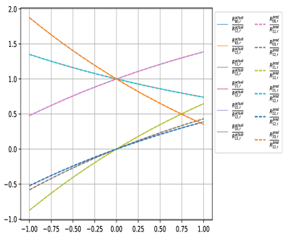
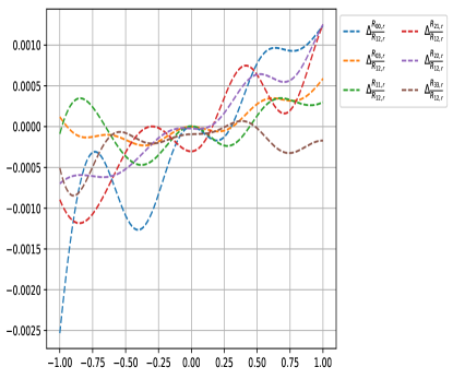
Figure 18: (a) 7-vertex model with Hamiltonian of type $H_{7v,2}$, with parameters $a_{1}=1,c_{1}=0.45,c_{2}=0.75,d_{1}=0.5$, (b)errors

8-vertex models have 3 gauge-inequivalent classes labelled $H_{8v,i},i=1,2,3$. One of these models, namely $H_{8v,1}$, is a generalisation of the XYZ model

$$H_{8v,1}=\begin{pmatrix}a_{1}&0&0&d_{1}\\ 0&b_{1}&c_{1}&0\\ 0&c_{1}&b_{1}&0\\ d_{2}&0&0&a_{1}\end{pmatrix}\,\leftrightarrow R_{8v,1}(u)=\begin{pmatrix}R_{8v,1}^{00}(u)&0&0&R_{8v,1}^{03}(u)\\ 0&R_{8v,1}^{11}(u)&R_{8v,1}^{12}(u)&0\\ 0&R_{8v,1}^{21}(u)&R_{8v,1}^{22}(u)&0\\ R_{8v,1}^{30}(u)&0&0&R_{8v,1}^{33}(u)\end{pmatrix}$$ (A.10)

where

$$\begin{split}R_{8v,1}^{00}(u)&=R_{8v,1}^{33}(u)=\frac{\mathrm{sn}{(u+2\eta,m)}}{\mathrm{sn}{(2\eta,m)}}e^{b_{1}u}\\ R_{8v,1}^{11}(u)&=R_{8v,1}^{22}(u)=\frac{\mathrm{sn}{(u,m)}}{\mathrm{sn}{(2\eta,m)}}e^{b_{1}u}\\ R_{8v,1}^{12}(u)&=R_{8v,1}^{21}(u)=e^{b_{1}u}\\ R_{8v,1}^{03}(u)&=\sqrt{\frac{d_{1}}{d_{2}}}\sqrt{m}\,\mathrm{sn}{(u+2\eta,m)}\mathrm{sn}{(u,m)}e^{b_{1}u}\\ R_{8v,1}^{30}(u)&=\sqrt{\frac{d_{2}}{d_{1}}}\sqrt{m}\,\mathrm{sn}{(u+2\eta,m)}\mathrm{sn}{(u,m)}e^{b_{1}u}\end{split}$$ (A.11)

with Hamiltonian coefficients given by

$$a_{1}=b_{1}+\frac{\mathrm{cn}(2\eta,m)\mathrm{dn}(2\eta,m)}{\mathrm{sn}(2\eta,m)}\,,\,\,c_{1}=\frac{1}{\mathrm{sn}(2\eta,m)}\,,\,\,d_{1}=\sqrt{m}\,\delta_{1}\,\mathrm{sn}(2\eta,m)\,,\,\,d_{2}=\sqrt{m}\,\delta_{2}\,\mathrm{sn}(2\eta,m)$$ (A.12)

for free parameters $b_{1},\eta,m,\delta_{1},\delta_{2}$. Figure 19 plots the predicted R-matrix components as ratios with respect to the $(12)$ component against the above analytic results, and their differences for a generic choice of parameters $b_{1}=0.4,\eta=0.8,m=0.5,\delta_{1}=1.3,\delta_{2}=0.7$.

[] []

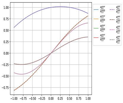
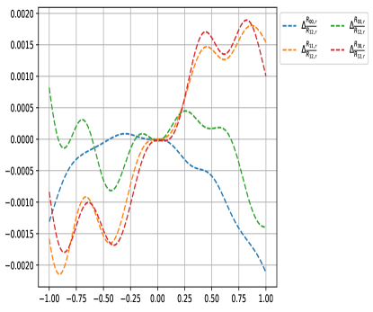
Figure 19: (a) 8-vertex model with Hamiltonian of type $H_{8v,1}$, with parameters $b_{1}=0.4,\eta=0.8,m=0.5,\delta_{1}=1.3,\delta_{2}=0.7$, (b)errors

The second class of 8-vertex XYZ-type solution has Hamiltonian $H_{8v,2}$ and R-matrix $R_{8v,2}(u)$ defined as follows

$$H_{8v,2}=\begin{pmatrix}a_{1}&0&0&d_{1}\\ 0&b_{1}&c_{1}&0\\ 0&c_{1}&b_{1}&0\\ d_{2}&0&0&2b_{1}-a_{1}\end{pmatrix}\leftrightarrow R_{8v,2}(u)=\begin{pmatrix}R_{8v,2}^{00}(u)&0&0&R_{8v,2}^{03}(u)\\ 0&R_{8v,2}^{11}(u)&R_{8v,2}^{12}(u)&0\\ 0&R_{8v,2}^{21}(u)&R_{8v,2}^{22}(u)&0\\ R_{8v,2}^{30}(u)&0&0&R_{8v,2}^{33}(u)\end{pmatrix}$$ (A.13)

where

$$\begin{split}R_{8v,2}^{00}(u)&=(\frac{\mathrm{cn}{(u,m)}}{\mathrm{dn}{(u,m)}}+\frac{\mathrm{sn}{(u,m)}\mathrm{cn}{(2\eta,m)}}{\mathrm{sn}{(2\eta,m)}})e^{b_{1}u}\\ R_{8v,2}^{11}(u)&=R_{8v,1}^{22}(u)=\frac{\mathrm{sn}{(u,m)}}{\mathrm{sn}{(2\eta,m)}}e^{b_{1}u}\\ R_{8v,2}^{12}(u)&=R_{8v,1}^{21}(u)=e^{b_{1}u}\\ R_{8v,2}^{03}(u)&=\frac{\delta_{1}}{\beta_{1}}\frac{\mathrm{sn}{(u,m)}\mathrm{cn}{(u,m)}}{\mathrm{dn}{(u,m)}\mathrm{sn}{(2\eta,m)}}e^{b_{1}u}\\ R_{8v,2}^{30}(u)&=\frac{\delta_{2}}{\beta_{1}}\frac{\mathrm{sn}{(u,m)}\mathrm{cn}{(u,m)}}{\mathrm{dn}{(u,m)}\mathrm{sn}{(2\eta,m)}}e^{b_{1}u}\\ R_{8v,2}^{33}(u)&=(\frac{\mathrm{cn}{(u,m)}}{\mathrm{dn}{(u,m)}}-\frac{\mathrm{sn}{(u,m)}\mathrm{cn}{(2\eta,m)}}{\mathrm{sn}{(2\eta,m)}})e^{b_{1}u}\end{split}$$ (A.14)

with the Hamiltonian coefficients given by

$$a_{1}=b_{1}+\frac{\mathrm{cn}(2\eta,m)}{\mathrm{sn}(2\eta,m)}\,,\,\,c_{1}=\frac{1}{\mathrm{sn}(2\eta,m)}\,,\,\,d_{1}=\frac{\delta_{1}}{\beta_{1}\mathrm{sn}(2\eta,m)}\,,\,\,d_{2}=\frac{\delta_{2}}{\beta_{1}\mathrm{sn}(2\eta,m)}$$ (A.15)

$$m=\frac{\delta_{1}\delta_{2}}{\alpha_{1}^{2}-\beta_{1}^{2}}\,,\,\,\mathrm{cn}(2\eta,m)=\frac{\alpha_{1}}{\beta_{1}}\,,\,\,\mathrm{sn}(2\eta,m)=\sqrt{1-\frac{\alpha_{1}^{2}}{\beta_{1}^{2}}}$$ (A.16)

for free parameters $b_{1},\alpha_{1},\beta_{1},\delta_{1},\delta_{2}$. Figure 20 plots the predicted R-matrix components as ratios with respect to the $(12)$ component against the above analytic results, and their differences for a generic choice of parameters $b_{1}=0.4,\alpha_{1}=0.5,\beta_{1}=0.7,\delta_{1}=0.3,\delta_{2}=0.2$.

[] []

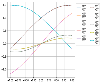
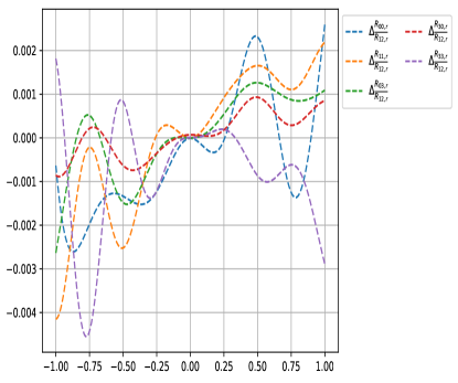
Figure 20: (a) 8-vertex model with Hamiltonian of type $H_{8v,2}$, with parameters $b_{1}=0.4,\alpha_{1}=0.5,\beta_{1}=0.7,\delta_{1}=0.3,\delta_{2}=0.2$, (b)errors

The second class of 8-vertex XYZ-type solution has Hamiltonian $H_{8v,3}$ and R-matrix $R_{8v,3}(u)$ defined as follows

$$H_{8v,3}=\begin{pmatrix}a_{1}&0&0&d_{1}\\ 0&a_{1}&-b_{1}&0\\ 0&b_{1}&a_{1}&0\\ d_{2}&0&0&a_{1}\end{pmatrix}\leftrightarrow R_{8v,3}(u)=\begin{pmatrix}R_{8v,3}^{00}(u)&0&0&R_{8v,3}^{03}(u)\\ 0&R_{8v,3}^{11}(u)&R_{8v,3}^{12}(u)&0\\ 0&R_{8v,3}^{21}(u)&R_{8v,3}^{22}(u)&0\\ R_{8v,3}^{30}(u)&0&0&R_{8v,3}^{33}(u)\end{pmatrix}$$ (A.17)

where

$$\begin{split}R_{8v,3}^{00}(u)&=R_{8v,1}^{33}(u)=\frac{\cosh{(b_{1}u)}}{\cos{(\sqrt{d_{1}d_{2}}u)}}e^{a_{1}u}\\ R_{8v,3}^{11}(u)&=-R_{8v,1}^{22}(u)=\frac{\sinh{(b_{1}u)}}{\cos{(\sqrt{d_{1}d_{2}}u)}}e^{a_{1}u}\\ R_{8v,3}^{12}(u)&=R_{8v,1}^{21}(u)=e^{a_{1}u}\\ R_{8v,3}^{03}(u)&=\sqrt{\frac{d_{1}}{d_{2}}}e^{a_{1}u}\tan{(\sqrt{d_{1}d_{2}}u)}\\ R_{8v,1}^{30}(u)&=\sqrt{\frac{d_{2}}{d_{1}}}e^{a_{1}u}\tan{(\sqrt{d_{1}d_{2}}u)}\end{split}$$ (A.18)

Figure 21 plots the predicted R-matrix components as ratios with respect to the $(12)$ component against the above analytic results, and their differences for a generic choice of parameters $a_{1}=1,\,b_{1}=-0.45,\,d_{1}=0.6,\,d_{2}=0.75$.

[] []

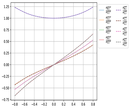
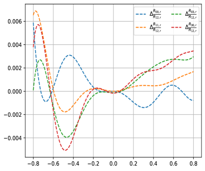
Figure 21: (a) 8-vertex model with Hamiltonian of type $H_{8v,3}$, with parameters $a_{1}=1,\,b_{1}=-0.45,\,d_{1}=0.6,\,d_{2}=0.75$, (b)errors

For non-XYZ type models, the 6 gauge-inequivalent Hamiltonians are of the form

$$H_{\mathrm{class}-1}=\begin{pmatrix}0&a_{1}&a_{2}&0\\ 0&a_{5}&0&a_{3}\\ 0&0&-a_{5}&a_{4}\\ 0&0&0&0\end{pmatrix}\,,\quad H_{\mathrm{class}-2}=\begin{pmatrix}0&a_{2}&a_{3}-a_{2}&a_{5}\\ 0&a_{1}&0&a_{4}\\ 0&0&-a_{1}&a_{3}-a_{4}\\ 0&0&0&0\end{pmatrix}\,,$$

$$H_{\mathrm{class}-3}=\begin{pmatrix}-a_{1}&(2a_{1}-a_{2})a_{3}&(2a_{1}+a_{2})a_{3}&0\\ 0&a_{1}-a_{2}&0&0\\ 0&0&a_{1}+a_{2}&0\\ 0&0&0&-a_{1}\end{pmatrix}\,,\quad H_{\mathrm{class}-4}=\begin{pmatrix}a_{1}&a_{2}&a_{2}&a_{3}\\ 0&-a_{1}&0&a_{4}\\ 0&0&-a_{1}&a_{4}\\ 0&0&0&a_{1}\end{pmatrix}\,,$$

$$H_{\mathrm{class}-5}=\begin{pmatrix}a_{1}&a_{2}&-a_{2}&0\\ 0&-a_{1}&2a_{1}&a_{3}\\ 0&2a_{1}&-a_{1}&-a_{3}\\ 0&0&0&a_{1}\end{pmatrix}\,,\quad H_{\mathrm{class}-6}=\begin{pmatrix}a_{1}&a_{2}&a_{2}&0\\ 0&-a_{1}&2a_{1}&-a_{2}\\ 0&2a_{1}&-a_{1}&-a_{2}\\ 0&0&0&a_{1}\end{pmatrix}$$ (A.19)

Corresponding R-matrices are

$$R_{\mathrm{class}-1}(u)=\begin{pmatrix}1&\frac{a_{1}(e^{a_{5}u}-1)}{a_{5}}&\frac{a_{2}(e^{a_{5}u}-1)}{a_{5}}&\frac{(a_{1}a_{3}+a_{2}a_{4})}{a_{5}^{2}}(\cosh{(a_{5}u)}-1)\\ 0&0&e^{-a_{5}u}&\frac{a_{4}(1-e^{-a_{5}u})}{a_{5}}\\ 0&e^{a_{5}u}&0&\frac{a_{3}(1-e^{-a_{5}u})}{a_{5}}\\ 0&0&0&1\end{pmatrix}$$ (A.20)

$$R_{\mathrm{class}-2}(u)=uP(\frac{a_{1}}{\sinh(a_{1}u)}+H_{class-5}+\frac{\tanh(a_{1}u)}{a_{1}}H_{class-5}^{2})\,,\quad P=\begin{pmatrix}1&0&0&0\\ 0&0&1&0\\ 0&1&0&0\\ 0&0&0&1\end{pmatrix}$$ (A.21)

$$R_{\mathrm{class}-3}(u)=\begin{pmatrix}e^{-a_{1}u}&a_{3}(e^{(a_{1}-a_{2})u}-e^{-a_{1}u})&a_{3}(e^{(a_{1}+a_{2})u}-e^{-a_{1}u})&0\\ 0&0&e^{(a_{1}+a_{2})u}&0\\ 0&e^{(a_{1}-a_{2})u}&0&0\\ 0&0&0&e^{-a_{1}u}\end{pmatrix}$$ (A.22)

$$R_{\mathrm{class}-4}(u)=\begin{pmatrix}e^{a_{1}u}&\frac{a_{2}\sinh{(a_{1}u)}}{a_{1}}&\frac{a_{2}\sinh{(a_{1}u)}}{a_{1}}&\frac{e^{a_{1}u}(a_{2}a_{4}+a_{1}a_{3}\coth{(a_{1}u)})\sinh^{2}{(a_{1}u)}}{a_{1}^{2}}\\ 0&0&e^{-a_{1}u}&\frac{a_{4}\sinh{(a_{1}u)}}{a_{1}}\\ 0&e^{-a_{1}u}&0&\frac{a_{4}\sinh{(a_{1}u)}}{a_{1}}\\ 0&0&0&e^{a_{1}u}\end{pmatrix}$$ (A.23)

$$R_{\mathrm{class}-5}(u)=(1-a_{1}u)\begin{pmatrix}2a_{1}u+1&a_{2}u&-a_{2}u&a_{2}a_{3}u^{2}\\ 0&2a_{1}u&1&-a_{3}u\\ 0&1&2a_{1}u&a_{3}u\\ 0&0&0&2a_{1}u+1\end{pmatrix}$$ (A.24)

$$R_{\mathrm{class}-6}(u)=(1-a_{1}u)\begin{pmatrix}2a_{1}u+1&a_{2}u(2a_{1}u+1)&a_{2}u(2a_{1}u+1)&-a_{2}^{2}u^{2}(2a_{1}u+1)\\ 0&2a_{1}u&1&-a_{2}u(2a_{1}u+1)\\ 0&1&2a_{1}u&-a_{2}u(2a_{1}u+1)\\ 0&0&0&2a_{1}u+1\end{pmatrix}$$ (A.25)

In the class-2 solution above, the non-zero R-matrix components are explicitly given by

$$\begin{split}R_{\mathrm{class}-2}^{00}(u)&=R_{\mathrm{class}-2}^{33}(u)=\frac{a_{1}u}{\sinh{u}}\\ R_{\mathrm{class}-2}^{01}(u)&=a_{2}u(1+\tanh{(\frac{a_{1}u}{2})})\,,\\ R_{\mathrm{class}-2}^{02}(u)&=(a_{2}-a_{3})u(-1+\tanh{(\frac{a_{1}u}{2})})\\ R_{\mathrm{class}-2}^{03}(u)&=a_{5}u(1+\frac{((a_{4}-a_{3})(a_{2}-a_{3})+a_{2}a_{4})\tanh{\frac{a_{1}u}{2}}}{a_{1}a_{5}})\\ R_{\mathrm{class}-2}^{12}(u)&=a_{1}u(-1+\frac{1}{\sinh(a_{1}u)}+\tanh{\frac{a_{1}u}{2}})\\ R_{\mathrm{class}-2}^{13}(u)&=(a_{4}-a_{3})u(-1+\tanh{(\frac{a_{1}u}{2})})\\ R_{\mathrm{class}-2}^{21}(u)&=a_{1}u(1+\frac{1}{\sinh(a_{1}u)}+\tanh{\frac{a_{1}u}{2}})\\ R_{\mathrm{class}-2}^{23}(u)&=a_{4}u(1+\tanh{(\frac{a_{1}u}{2})})\end{split}$$ (A.26)

Amongst the above non-XYZ type models, we have already looked into the training for Class 1 model in section 4.1. Figure 22, 23, 24 plot the training vs actual R-matrix components for classes 2,3,4, class 5, and class 6 respectively, with generic Hamiltonian parameters. Also we note that allowing for complex parameters results in generically complex R-matrices. We compare the predictions against the actual formulae by taking ratios with respect to the real part of the (00) component for classes 2-5, and (12) component for class 6.

[] []
[] []

[] []

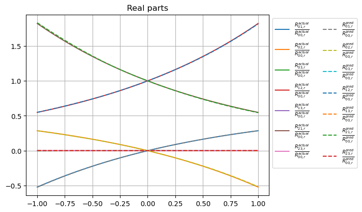
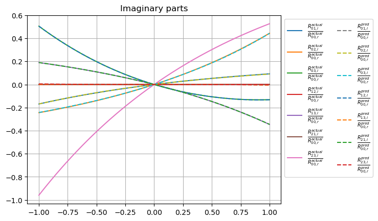
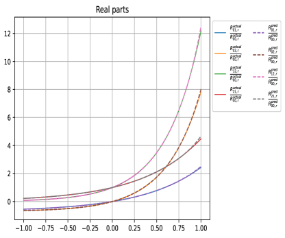
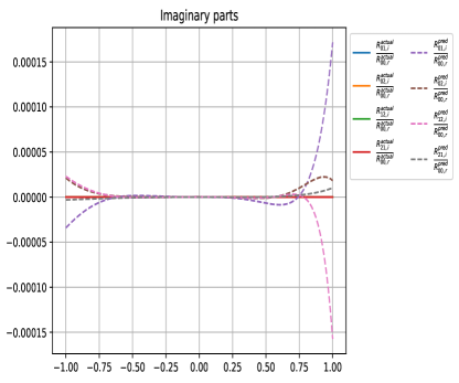
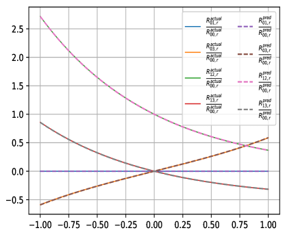
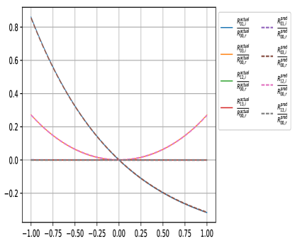
Figure 22: (a,b) class 2, with $H_{2}$ parameters $a_{1}=-0.6,\,a_{2}=0.381+0.123\,i,\,a_{3}=0.447\,i,\,a_{4}=0.7\,i,\,a_{5}=-0.3\,i$: real and imaginary parts, (c,d) class 3, with $H_{2}$ parameters $a_{1}=1,\,a_{2}=0.5,\,a_{3}=0.7$: real and imaginary parts, (e,f) class 4, with $H_{2}$ parameters $a_{1}=0.5,\,a_{2}=-0.5\,i,\,a_{3}=0.5,\,a_{4}=-0.5$: real and imaginary parts

[] []

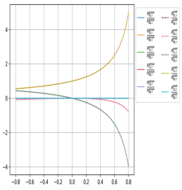
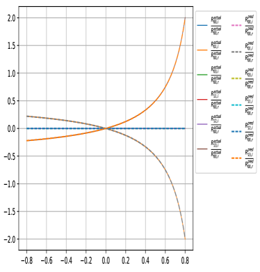
Figure 23: (a,b) class 5, with $H_{2}$ parameters $a_{1}=-0.5,\,a_{2}=-0.5\,i,\,a_{3}=-0.5\,i$: real and imaginary parts

[] []

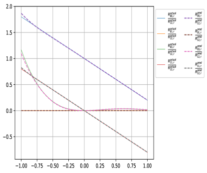
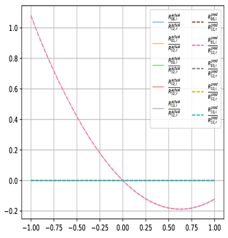
Figure 24: (a,b) class 6, with $H_{2}$ parameters $a_{1}=-0.4,\,a_{2}=-0.6\,i$: real and imaginary parts

Appendix B Designing the Neural Network

This appendix contains an extensive overview of the architecture of our neural network solver, as well as details of the hyperparameters with which the network is trained. Our starting point is the close analogy between our problem of machine learning R-matrices by imposing constraints and the design of the Siamese Neural Networks [79, 80]. These were designed to function in settings where the canonical supervised learning approach of (3.5) for classification becomes infeasible due to the large number of target classes $\left\{y\right\}$ and the paucity of training examples $\left\{x_{\alpha}\right\}$ corresponding to each class $y_{\alpha}$. In such a situation, one may instead define a similarity relation

$$x_{\alpha_{1}}\sim x_{\alpha_{2}}\qquad\iff\qquad y\left(x_{\alpha_{1}}\right)=y\left(x_{\alpha_{2}}\right),$$ (B.1)

and train the neural network to learn a function $\phi\left(x\right):\mathbb{R}^{D}\rightarrow\mathbb{R}^{d}$ such that the Euclidean distance between representatives $\phi\left(x\right)$ of two input vectors $x_{1}$, $x_{2}$ that are similar to each other is small, while the distance between dissimilar data is large. Schematically,

$$d\left(x_{a},x_{b}\right)=\left|\phi\left(x_{a}\right)-\phi\left(x_{b}\right)\right|^{2}\approx 0\qquad\iff\qquad x_{a}\sim x_{b}\,.$$ (B.2)

This is visualized in Figure 25.

Figure 25: Visualizing the map $\phi$ which is learnt by the Siamese architecture. The points $x_{1}$ and $x_{3}$ are similar to each other while $x_{2}$ is dissimilar to both of them.

There are many loss functions by which such networks may be trained, see for example [79, 80, 81, 82]. For definiteness, we mention the contrastive loss function of [79, 80], given by

$$\mathcal{L}=Yd\left(x_{1},x_{2}\right)+\left(1-Y\right)\max\left(r_{o}-d\left(x_{1},x_{2}\right),0\right)\,,$$ (B.3)

where $Y=1$ if $x_{1}\sim x_{2}$ and $Y=0$ otherwise. Clearly this loss function causes the network to learn a function $\phi$ such that similar inputs $x$ are clustered together while dissimilar inputs are pushed at least a distance $r_{o}$ apart. This therefore realizes our naive criterion for $\phi$ laid out in Equation (B.2). We also see very explicitly that the loss function in Equation (B.3) does not directly depend on the values $y$ in contrast to Equation (3.5). Instead, the network is trained to learn a function $\phi\left(x\right)$ which obeys a property which is not given point-wise for each input $x$ but instead is expressed as a non-linear constraint (B.2) on $\phi\left(x\right)$ evaluated at two points $x_{1}$ and $x_{2}$.

B.1 The Neural Network Architecture and Forward Propagation

We now provide some more details about our implementation of $\mathcal{R}\left(u\right)$ and the training done to converge to solutions of the Yang-Baxter equation (2.3) consistent with additional requirements such as regularity (2.4). As already mentioned in Section 3.2, each matrix element $\mathcal{R}_{ij}$ is decomposed into the sum $a_{ij}+i\,b_{ij}$ which are individually modeled by MLPs. In principle each MLP is independent of the rest and can be individually designed. We shall however take all MLPs to contain two hidden layers of 50 neurons each, followed by a single output neuron which is linear activated . The possible activations for the hidden layers are compared in Appendix B.2 below. To proceed further, note that our loss function involves a term (3.7) which takes arguments $\mathcal{R}\left(u\right)$, $\mathcal{R}\left(v\right)$ and $\mathcal{R}\left(u-v\right)$ where $u$, $v$ are valued in $\Omega$. This clearly has a very strong parallel with the Siamese Networks introduced above. At least intuitively, one may regard our problem as training a `triplet' of identical neural networks $\mathcal{R}$ to optimize the loss function (3.7). In addition however, we also have to train the function on loss functions such as (3.12) and (3.13). These constraints, along with the Siamese schematic shown in Figure 25 motivate our design visualized in Figure 26.

Figure 26: Visualizing the forward propagation of the neural network $\mathcal{R}\left(u\right)$. This has a very strong parallel to Figure 25, with the function $\mathcal{R}\left(u\right)$ playing the role of the map $\phi$. The only difference is that $\mathcal{R}\left(u\right)$ also has additional constraints on $\mathcal{R}\left(0\right)$ and $\mathcal{R}^{\prime}\left(0\right)$ which are unique to our problem.

During the forward propagation we sample a minibatch of $u$ and $v$ values, from which the corresponding $u-v$ is constructed. Next, the $\mathcal{R}$ matrix is constructed at $u$, $v$ and $u-v$ via Equation (3.6). We also evaluate $\mathcal{R}\left(0\right)$ and $\mathcal{R}^{\prime}\left(0\right)$ thus completing the forward propagation. Next, we compute the losses (3.7), (3.12) and (3.13) as well as possibly (3.15). The loss function is trained on by using the Adam optimizer [63], with an initial learning rate $\eta$ of $10^{-3}$ which is annealed to $10^{-8}$ in steps of $10^{-1}$ by monitoring the saturation in the Yang-Baxter loss computed for the validation set over 5-10 epochs. The effect of this annealing in the learning rate is also visible in the training histories in Figures 2 and 27 where the step-wise falls in the losses correspond to the drops in the learning rate. Across the board, training converges in about 100 epochs and is terminated by early stopping.

B.2 Comparing different activation functions

We now turn to a brief comparison of the performance of different activation functions with the above set up. Again for uniformity, we will use one activation throughout for all the MLPs $a_{ij}$ and $b_{ij}$, but for the output neuron which is linearly activated. We then compared the performance of this neural network architecture while learning the Hamiltonian

$$H_{6v,1}=\begin{pmatrix}0.3&0&0&0\\ 0&0.45&0.4&0\\ 0&0.25&0.6&0\\ 0&0&0&0.3\end{pmatrix}\,,$$ (B.4)

which is 6-vertex Type 1 in the classification of [58], see Equation (A.2) above. The neural network was trained with the loss functions (3.7), (3.13) and (3.12) and setting $\lambda_{H}$ and $\lambda_{reg}$ to 1 each. The training was carried out for 200 epochs on observing that the networks did not perform better on training for longer. Further, we set a batch size of 16 and optimized using Adam with a starting learning rate of $10^{-3}$ which was annealed to $10^{-8}$ using the saturation in the Yang-Baxter loss over the validation set as the criterion as mentioned above. We conducted this training using the activations sigmoid, tanh, swish, all of which are holomorphic, as well as elu and relu. The last two are not holomorphic but have been included for completeness. The evolution of the Yang-Baxter and the Hamiltonian loss for all these activations is shown in Figure 27 and Table 1.

Activation	Final Yang-Baxter Loss	Final Hamiltonian Loss	Saturation Epoch
sigmoid	$2.5\times 10^{-3}$	$6.12\times 10^{-7}$	150
tanh	$1.90\times 10^{-4}$	$5.25\times 10^{-7}$	125
swish	$6.49\times 10^{-5}$	$1.51\times 10^{-7}$	75
elu	$2.75\times 10^{-4}$	$5.63\times 10^{-7}$	100
relu	$5.52\times 10^{-4}$	$4.63\times 10^{-7}$	100

Table 1: Performance of different activation functions on learning the Hamiltonian (B.4). The saturation epoch is the approximate epoch after which the model did not train further. The final values of the Yang-Baxter and Hamiltonian losses after saturation is also mentioned. We observed that the swish activation converges sooner and to lower losses. This is stable across multiple runs. See also Figure 27.

[] []

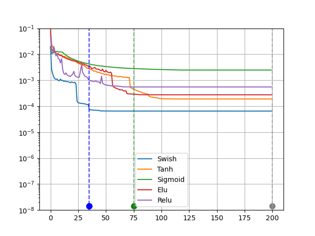
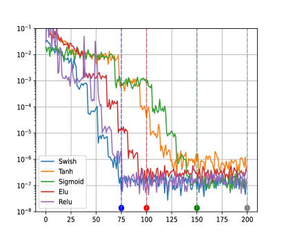
Figure 27: The evolution of the Yang-Baxter loss (left) and the Hamiltonian loss (right) for a variety of activation functions when training for 200 epochs. The swish activation tends to outperform the others. The precise numbers are given in Table 1.

On the whole, we see that the swish activation tends to outperform the others quite significantly. While these are the results of a single run, we found that the result is consistent across several runs and tasks, leading us to adopt the swish activation uniformly across the board for all the analyses shown in this paper.

B.3 Proof of Concept: Training with a single hidden neuron.

As a final observation we present a simple proof of concept of our approach of solving the Yang-Baxter equation along with other constraints by optimizing suitable loss functions. Here, instead of attempting to deep learn the solution, we use a single layer of neurons for each R-matrix function and pick an activation function by the form of the known analytic solution. In effect, rather than rely on the feature learning properties of a deep MLP as we have done in the rest of our paper, we ourselves provide activation functions which should furnish a natural basis to express the known analytic solutions in.

For definiteness, consider the XXZ model at $\eta=\frac{\pi}{3}$. The non-zero entries in this R-matrix are

$$R_{00}(u)=\sin{(u+\eta)}\,,\qquad R_{11}(u)=\sin{(u-\eta)}=R_{22}(u)\,,\qquad R_{12}(u)=\sin\left(\eta\right)=R_{21}\left(u\right)\,,$$ (B.5)

as may be observed by setting $m=0$ in Equation (4.4). We define the networks $a_{ij}$ and $b_{ij}$ to have a single hidden layer of a solitary neuron activated by the sin function. This means that the functions learnt by the network are simply of the form

$$a_{ij}=\tilde{W}\circ\texttt{sin}\left(W\circ u\right)\,,$$ (B.6)

and similarly for the $b_{ij}$. The $W$ and $\tilde{W}$ are the weight and bias of the hidden and the output neuron respectively and the composition $W\circ u$ is shorthand for the affine transformation $w\,u+b$. Next, we train the network imposing the losses (3.7), (3.12), (3.13) and (3.15), each with weight $\lambda=1$, and the Adam optimizer with our standard learning rate scheduling. Figure 28 plots the trained XXZ $R$-matrix components for $u$ lying in the range (-10,10).

[] [] .

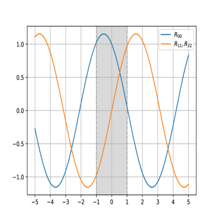
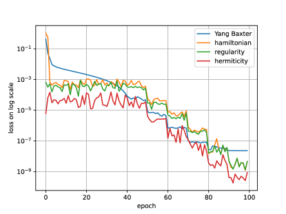
Figure 28: The figure on the left shows the XXZ model R-matrix with $\eta=\frac{\pi}{3}$ obtained by trained on a single sin activated hidden neuron in the range $u\in(-1,1)$ shown in gray. The solution remains valid outside the training domain as well. The figure on the right shows the corresponding training curves.

Note that since we trained with an activation function that presupposed our knowlege of the exact solution – in effect, the true R-matrix lay within our hypothesis class – the model trained to losses of the order of $10^{-8}$ which is several orders of magnitude below the typical end of training losses we observed in the standardized framework. Further, we also obtain an excellent performance even out of the domain of training, which is usually not the case in machine learning.

References

- [1] Y. LeCun, Y. Bengio and G. Hinton, ``Deep learning'', nature 521, 436 (2015).
- [2] Y.-H. He, ``Machine-learning the string landscape'', Physics Letters B 774, 564 (2017), https://www.sciencedirect.com/science/article/pii/S0370269317308365.
- [3] J. Carifio, J. Halverson, D. Krioukov and B. D. Nelson, ``Machine learning in the string landscape'', Journal of High Energy Physics 2017, 1 (2017).
- [4] D. Krefl and R.-K. Seong, ``Machine learning of Calabi-Yau volumes'', Physical Review D 96, 066014 (2017).
- [5] F. Ruehle, ``Evolving neural networks with genetic algorithms to study the String Landscape'', Journal of High Energy Physics 2017, 1 (2017).
- [6] C. R. Brodie, A. Constantin, R. Deen and A. Lukas, ``Machine Learning Line Bundle Cohomology'', Fortsch. Phys. 68, 1900087 (2020), arxiv:1906.08730.
- [7] R. Deen, Y.-H. He, S.-J. Lee and A. Lukas, ``Machine learning string standard models'', Phys. Rev. D 105, 046001 (2022), arxiv:2003.13339.
- [8] Y.-H. He and A. Lukas, ``Machine Learning Calabi-Yau Four-folds'', Phys. Lett. B 815, 136139 (2021), arxiv:2009.02544.
- [9] H. Erbin and R. Finotello, ``Machine learning for complete intersection Calabi-Yau manifolds: a methodological study'', Phys. Rev. D 103, 126014 (2021), arxiv:2007.15706.
- [10] H. Erbin, R. Finotello, R. Schneider and M. Tamaazousti, ``Deep multi-task mining Calabi–Yau four-folds'', Mach. Learn. Sci. Tech. 3, 015006 (2022), arxiv:2108.02221.
- [11] X. Gao and H. Zou, ``Applying machine learning to the Calabi-Yau orientifolds with string vacua'', Phys. Rev. D 105, 046017 (2022), arxiv:2112.04950.
- [12] A. Ashmore, L. Calmon, Y.-H. He and B. A. Ovrut, ``Calabi-Yau Metrics, Energy Functionals and Machine-Learning'', International Journal of Data Science in the Mathematical Sciences 1, 49 (2023), arxiv:2112.10872.
- [13] L. B. Anderson, M. Gerdes, J. Gray, S. Krippendorf, N. Raghuram and F. Ruehle, ``Moduli-dependent Calabi-Yau and SU (3)-structure metrics from Machine Learning'', Journal of High Energy Physics 2021, 1 (2021).
- [14] M. Douglas, S. Lakshminarasimhan and Y. Qi, ``Numerical Calabi-Yau metrics from holomorphic networks'', in: ``Mathematical and Scientific Machine Learning'', 223–252p.
- [15] M. Larfors, A. Lukas, F. Ruehle and R. Schneider, ``Numerical metrics for complete intersection and Kreuzer–Skarke Calabi–Yau manifolds'', Mach. Learn. Sci. Tech. 3, 035014 (2022), arxiv:2205.13408.
- [16] Y.-H. He, S. Lal and M. Z. Zaz, ``The World in a Grain of Sand: Condensing the String Vacuum Degeneracy'', arxiv:2111.04761.
- [17] A. Morningstar and R. G. Melko, ``Deep learning the ising model near criticality'', arxiv:1708.04622.
- [18] Y. Zhang, R. G. Melko and E.-A. Kim, ``Machine learning Z 2 quantum spin liquids with quasiparticle statistics'', Physical Review B 96, 245119 (2017).
- [19] H.-Y. Chen, Y.-H. He, S. Lal and M. Z. Zaz, ``Machine Learning Etudes in Conformal Field Theories'', arxiv:2006.16114.
- [20] E.-J. Kuo, A. Seif, R. Lundgren, S. Whitsitt and M. Hafezi, ``Decoding conformal field theories: From supervised to unsupervised learning'', Phys. Rev. Res. 4, 043031 (2022), arxiv:2106.13485.
- [21] P. Basu, J. Bhattacharya, D. P. S. Jakka, C. Mosomane and V. Shukla, ``Machine learning of Ising criticality with spin-shuffling'', arxiv:2203.04012.
- [22] K. Shiina, H. Mori, Y. Okabe and H. K. Lee, ``Machine-learning studies on spin models'', Scientific reports 10, 2177 (2020).
- [23] X. Han and S. A. Hartnoll, ``Deep Quantum Geometry of Matrices'', Phys. Rev. X 10, 011069 (2020), arxiv:1906.08781.
- [24] W. E and B. Yu, ``The Deep Ritz method: A deep learning-based numerical algorithm for solving variational problems'', arxiv:1710.00211.
- [25] M. Raissi, P. Perdikaris and G. E. Karniadakis, ``Physics Informed Deep Learning (Part I): Data-driven Solutions of Nonlinear Partial Differential Equations'', arxiv:1711.10561.
- [26] G. Lample and F. Charton, ``Deep Learning for Symbolic Mathematics'', arxiv:1912.01412.
- [27] A. Davies, P. Veličković, L. Buesing, S. Blackwell, D. Zheng, N. Tomašev, R. Tanburn, P. Battaglia, C. Blundell, A. Juhász, M. Lackenby, G. Williamson, D. Hassabis and P. Kohli, ``Advancing mathematics by guiding human intuition with AI'', Nature 600, 70 (2021).
- [28] Y.-H. He, ``Machine-Learning Mathematical Structures'', arxiv:2101.06317.
- [29] S.-M. Udrescu and M. Tegmark, ``AI Feynman: A physics-inspired method for symbolic regression'', Science Advances 6, eaay2631 (2020).
- [30] G. Cybenko, ``Approximation by superpositions of a sigmoidal function'', Mathematics of control, signals and systems 2, 303 (1989).
- [31] K. Hornik, M. Stinchcombe and H. White, ``Multilayer feedforward networks are universal approximators'', Neural networks 2, 359 (1989).
- [32] Z. Lu, H. Pu, F. Wang, Z. Hu and L. Wang, ``The expressive power of neural networks: A view from the width'', Advances in neural information processing systems 30, (2017).
- [33] M. Telgarsky, ``Representation benefits of deep feedforward networks'', arxiv:1509.08101.
- [34] X. Glorot and Y. Bengio, ``Understanding the difficulty of training deep feedforward neural networks'', Proceedings of the thirteenth international conference on artificial intelligence and statistics , 249 (2010).
- [35] G. E. Hinton, N. Srivastava, A. Krizhevsky, I. Sutskever and R. R. Salakhutdinov, ``Improving neural networks by preventing co-adaptation of feature detectors'', arxiv:1207.0580.
- [36] N. Srivastava, G. Hinton, A. Krizhevsky, I. Sutskever and R. Salakhutdinov, ``Dropout: a simple way to prevent neural networks from overfitting'', The journal of machine learning research 15, 1929 (2014).
- [37] S. Ioffe and C. Szegedy, ``Batch normalization: Accelerating deep network training by reducing internal covariate shift'', in: ``International conference on machine learning'', 448–456p.
- [38] L. N. Smith, ``A disciplined approach to neural network hyper-parameters: Part 1–learning rate, batch size, momentum, and weight decay'', arxiv:1803.09820.
- [39] H. Zhang, Y. N. Dauphin and T. Ma, ``Fixup initialization: Residual learning without normalization'', arxiv:1901.09321.
- [40] F. Chollet et al., ``Keras: The python deep learning library'', Astrophysics source code library , ascl (2018).
- [41] M. Abadi, A. Agarwal, P. Barham, E. Brevdo, Z. Chen, C. Citro, G. S. Corrado, A. Davis, J. Dean, M. Devin, S. Ghemawat, I. Goodfellow, A. Harp, G. Irving, M. Isard, Y. Jia, R. Jozefowicz, L. Kaiser, M. Kudlur, J. Levenberg, D. Mané, R. Monga, S. Moore, D. Murray, C. Olah, M. Schuster, J. Shlens, B. Steiner, I. Sutskever, K. Talwar, P. Tucker, V. Vanhoucke, V. Vasudevan, F. Viégas, O. Vinyals, P. Warden, M. Wattenberg, M. Wicke, Y. Yu and X. Zheng, ``TensorFlow: Large-Scale Machine Learning on Heterogeneous Systems'', Software available from tensorflow.org, https://www.tensorflow.org/.
- [42] A. Paszke, S. Gross, F. Massa, A. Lerer, J. Bradbury, G. Chanan, T. Killeen, Z. Lin, N. Gimelshein, L. Antiga, A. Desmaison, A. Kopf, E. Yang, Z. DeVito, M. Raison, A. Tejani, S. Chilamkurthy, B. Steiner, L. Fang, J. Bai and S. Chintala, ``PyTorch: An Imperative Style, High-Performance Deep Learning Library'', in: ``Advances in Neural Information Processing Systems 32'', Curran Associates, Inc. (2019), 8024–8035p.
- [43] Z. Liu and M. Tegmark, ``Machine learning hidden symmetries'', Physical Review Letters 128, 180201 (2022).
- [44] Z. Liu and M. Tegmark, ``Machine learning conservation laws from trajectories'', Physical Review Letters 126, 180604 (2021).
- [45] R. Bondesan and A. Lamacraft, ``Learning symmetries of classical integrable systems'', arxiv:1906.04645.
- [46] S. J. Wetzel, R. G. Melko, J. Scott, M. Panju and V. Ganesh, ``Discovering symmetry invariants and conserved quantities by interpreting siamese neural networks'', Phys. Rev. Res. 2, 033499 (2020), https://link.aps.org/doi/10.1103/PhysRevResearch.2.033499.
- [47] R. T. Forestano, K. T. Matchev, K. Matcheva, A. Roman, E. Unlu and S. Verner, ``Deep Learning Symmetries and Their Lie Groups, Algebras, and Subalgebras from First Principles'', arxiv:2301.05638.
- [48] G. F. Chew, ``S-matrix theory of strong interactions without elementary particles'', Reviews of Modern Physics 34, 394 (1962).
- [49] R. J. Eden, P. V. Landshoff, D. I. Olive and J. C. Polkinghorne, ``The analytic S-matrix'', Cambridge Univ. Press (1966), Cambridge.
- [50] M. Kruczenski, J. Penedones and B. C. van Rees, ``Snowmass White Paper: S-matrix Bootstrap'', arxiv:2203.02421.
- [51] M. F. Paulos, J. Penedones, J. Toledo, B. C. van Rees and P. Vieira, ``The S-matrix bootstrap II: two dimensional amplitudes'', JHEP 1711, 143 (2017), arxiv:1607.06110.
- [52] M. F. Paulos, J. Penedones, J. Toledo, B. C. van Rees and P. Vieira, ``The S-matrix bootstrap. Part III: higher dimensional amplitudes'', JHEP 1912, 040 (2019), arxiv:1708.06765.
- [53] Y. He, A. Irrgang and M. Kruczenski, ``A note on the S-matrix bootstrap for the 2d O(N) bosonic model'', JHEP 1811, 093 (2018), arxiv:1805.02812.
- [54] A. B. Zamolodchikov and A. B. Zamolodchikov, ``Relativistic Factorized S Matrix in Two-Dimensions Having O(N) Isotopic Symmetry'', JETP Lett. 26, 457 (1977).
- [55] P. P. Kulish, N. Y. Reshetikhin and E. K. Sklyanin, ``Yang-Baxter Equation and Representation Theory. 1.'', Lett. Math. Phys. 5, 393 (1981).
- [56] M. Jimbo, ``Quantum r Matrix for the Generalized Toda System'', Commun. Math. Phys. 102, 537 (1986).
- [57] R. Vieira, ``Solving and classifying the solutions of the Yang-Baxter equation through a differential approach. Two-state systems'', Journal of High Energy Physics 2018, 1 (2018).
- [58] M. De Leeuw, A. Pribytok and P. Ryan, ``Classifying integrable spin-1/2 chains with nearest neighbour interactions'', Journal of Physics A: Mathematical and Theoretical 52, 505201 (2019).
- [59] M. de Leeuw, C. Paletta, A. Pribytok, A. L. Retore and P. Ryan, ``Classifying Nearest-Neighbor Interactions and Deformations of AdS'', Phys. Rev. Lett. 125, 031604 (2020), arxiv:2003.04332.
- [60] M. de Leeuw, C. Paletta, A. Pribytok, A. L. Retore and P. Ryan, ``Yang-Baxter and the Boost: splitting the difference'', SciPost Phys. 11, 069 (2021), arxiv:2010.11231.
- [61] S. Krippendorf, D. Lust and M. Syvaeri, ``Integrability Ex Machina'', Fortsch. Phys. 69, 2100057 (2021), arxiv:2103.07475.
- [62] P. Ramachandran, B. Zoph and Q. V. Le, ``Searching for activation functions'', arxiv:1710.05941.
- [63] D. P. Kingma and J. Ba, ``Adam: A method for stochastic optimization'', arxiv:1412.6980.
- [64] K. He, X. Zhang, S. Ren and J. Sun, ``Deep residual learning for image recognition'', in: ``Proceedings of the IEEE conference on computer vision and pattern recognition'', 770–778p.
- [65] M. Tetel'man, ``Lorentz group for two-dimensional integrable lattice systems'', Soviet Journal of Experimental and Theoretical Physics 55, 306 (1982).
- [66] J. Hoffman, D. A. Roberts and S. Yaida, ``Robust learning with jacobian regularization'', arxiv:1908.02729.
- [67] S. Park, C. Yun, J. Lee and J. Shin, ``Minimum width for universal approximation'', arxiv:2006.08859.
- [68] A. Choromanska, M. Henaff, M. Mathieu, G. B. Arous and Y. LeCun, ``The loss surfaces of multilayer networks'', in: ``Artificial intelligence and statistics'', 192–204p.
- [69] Y. N. Dauphin, R. Pascanu, C. Gulcehre, K. Cho, S. Ganguli and Y. Bengio, ``Identifying and attacking the saddle point problem in high-dimensional non-convex optimization'', Advances in neural information processing systems 27, (2014).
- [70] L. Takhtadzhan and L. D. Faddeev, ``The quantum method of the inverse problem and the Heisenberg XYZ model'', Russian Mathematical Surveys 34, 11 (1979).
- [71] S. Lal, S. Majumder and E. Sobko, ``Drawing the Map of Integrable Spin Chains'', in progress , .
- [72] N. Beisert and M. Staudacher, ``The N= 4 SYM integrable super spin chain'', Nuclear Physics B 670, 439 (2003).
- [73] R. Borsato, O. O. Sax, A. Sfondrini, B. Stefanski and A. Torrielli, ``The all-loop integrable spin-chain for strings on AdS3 S 3 T 4: the massive sector'', Journal of High Energy Physics 2013, 1 (2013).
- [74] S. Majumder, O. O. Sax, B. Stefański and A. Torrielli, ``Protected states in AdS3 backgrounds from integrability'', Journal of Physics A: Mathematical and Theoretical 54, 415401 (2021).
- [75] S. Frolov and A. Sfondrini, ``Mirror thermodynamic Bethe ansatz for AdS3/CFT2'', Journal of High Energy Physics 2022, 1 (2022).
- [76] M. Schmidt and H. Lipson, ``Distilling free-form natural laws from experimental data'', science 324, 81 (2009).
- [77] R. Quessard, T. Barrett and W. Clements, ``Learning disentangled representations and group structure of dynamical environments'', Advances in Neural Information Processing Systems 33, 19727 (2020).
- [78] M. F. Paulos and Z. Zheng, ``Bounding scattering of charged particles in dimensions'', JHEP 2005, 145 (2020), arxiv:1805.11429.
- [79] J. Bromley, J. W. Bentz, L. Bottou, I. Guyon, Y. LeCun, C. Moore, E. Säckinger and R. Shah, ``Signature verification using a ``siamese" time delay neural network'', International Journal of Pattern Recognition and Artificial Intelligence 7, 669 (1993).
- [80] R. Hadsell, S. Chopra and Y. LeCun, ``Dimensionality reduction by learning an invariant mapping'', in: ``2006 IEEE Computer Society Conference on Computer Vision and Pattern Recognition (CVPR'06)'', 1735–1742p.
- [81] G. Chechik, V. Sharma, U. Shalit and S. Bengio, ``Large Scale Online Learning of Image Similarity Through Ranking.'', Journal of Machine Learning Research 11, (2010).
- [82] F. Schroff, D. Kalenichenko and J. Philbin, ``Facenet: A unified embedding for face recognition and clustering'', in: ``Proceedings of the IEEE conference on computer vision and pattern recognition'', 815–823p.