What does self-attention learn from Masked Language Modelling?

Abstract

Transformers are neural networks which revolutionised natural language processing and machine learning. They process sequences of inputs, like words, using a mechanism called self-attention, which is trained via masked language modelling (MLM). In MLM, a word is randomly masked in an input sequence, and the network is trained to predict the missing word. Despite the practical success of transformers, it remains unclear what type of data distribution self-attention can learn efficiently. Here, we show analytically that if one decouples the treatment of word positions and embeddings, a single layer of self-attention learns the conditionals of a generalised Potts model with interactions between sites and Potts colours. Moreover, we show that training this neural network is exactly equivalent to solving the inverse Potts problem by the so-called pseudo-likelihood method, well known in statistical physics. Using this mapping, we compute the generalisation error of self-attention in a model scenario analytically using the replica method.

Introduction.

Transformers Vaswani et al. (2017) are a powerful type of neural network that have achieved state-of-the art results in natural language processing (NLP) Devlin et al. (2019); Howard and Ruder (2018); Radford et al. (2018); Brown et al. (2020); OpenAI (2023), image classification Dosovitskiy et al. (2021), and even protein structure prediction Jumper et al. (2021). While standard neural networks can be thought of as functions of a single input, transformers act on sets of “tokens”, like words in a sentence. The key to the success of transformers is a technique called masked language modelling (MLM), where transformers are trained to predict missing words in a sentence Devlin et al. (2019); Howard and Ruder (2018); Radford et al. (2018); Brown et al. (2020); OpenAI (2023), cf. fig. 1a. This technique has the advantage that it can leverage large amounts of raw text (or images, or protein sequences) without any annotation. By learning the conditional distribution of having a word in a specific position of the sentence, given the other words, transformers ostensibly learn the relationships between words in a robust way.

The basic building block of transformers is the self-attention (SA) mechanism Bahdanau et al. (2016); Kim et al. (2017), which transforms a sequence of tokens ${\mathbf{x}}_{j}$ into another sequence ${\mathbf{h}}_{j}$. We illustrate self-attention on a masked language modelling task in fig. 1. The sentence is first transformed into a set of representations ${\mathbf{x}}_{j}={\mathbf{e}}_{j}+{\mathbf{p}}_{j}$, where ${\mathbf{e}}_{j}$ is a vector representing the $j$th word and the vector ${\mathbf{p}}_{j}$ encodes its position. SA then computes a linear transformation of the representations to yield the values ${\mathbf{v}}_{j}$. The $k$th output vector ${\mathbf{h}}_{k}$ is then a linear combination of the values ${\mathbf{v}}_{j}$ weighted by an attention matrix $A$, whose elements $A_{kj}$ quantify the relative importance of the $j$th input token for the $k$th output vector, for example based on their semantic similarity. The functions to compute values ${\mathbf{v}}_{j}$ and the attention matrix $A$ both have trainable parameters, see eq. 2 for a precise definition. The flexibility of self-attention comes from the attention weights $A_{kj}$, which are not fixed, but computed given the context, i.e. the surrounding tokens.

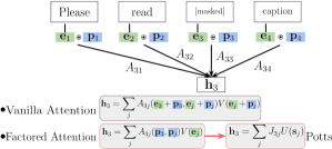
Figure 1: Masked language modelling (MLM) with a single layer of self-attention. The goal of MLM is to predict the masked word in a given sentence. Self-attention first maps words into representations ${\mathbf{e}}_{j}+{\mathbf{p}}_{j}$, where ${\mathbf{e}}_{j}$ are embedding vectors representing words, and ${\mathbf{p}}_{j}$ encode their positions. For a given masked word, the associated attention vector ${\mathbf{h}}_{k}$ is computed as a linear combination of the values ${\mathbf{v}}_{j}=V({\mathbf{e}}_{j}+{\mathbf{p}}_{j})$ of all other tokens, weighted by the attention weights $A_{kj}$. In vanilla self-attention, values and attention weights depend on embeddings and positional vectors, while in factored attention, attention weights depend only on positions, and values only on the embeddings. By identifying the attention weights $A$ with the interaction matrix $J$ of a Potts model eq. 1, the value matrix $V$ with the colour similarity matrix U and the embedding vectors with the one-hot spins, we get a learning model identical to a Potts model.

The practical success of transformers raises several fundamental questions: what are the statistical structures that self-attention learns with MLM? More precisely, since the MLM objective is to learn the conditional probability distribution of words given a set of surrounding words, which family of conditional probabilities can self-attention learn? And how many samples are required to achieve good performance? Here, we make a step towards answering these questions by exploiting tools from the statistical physics of learning Gardner and Derrida (1989); Seung et al. (1992); Engel and Van den Broeck (2001); Carleo et al. (2019).

The first challenge is to design a data model that mimics the structure of real sentences. While classical works modelled inputs as vectors of i.i.d. random variables, recent work has introduced more sophisticated data models for neural networks Chung et al. (2018); Goldt et al. (2020a); Spigler et al. (2020); Gerace et al. (2021); Favero et al. (2022); Loureiro et al. (2022); Ingrosso and Goldt (2022) which allowed the study of unsupervised learning Refinetti and Goldt (2022); Cui and Zdeborová (2023). To analyse the self-supervised learning of MLM, we model sequences of words as system of spins, interacting via a generalised Potts Hamiltonian Potts (1952); Wu (1982) with couplings between colours (=words) and positions. We sample a synthetic data set from the Potts model using Monte Carlo and perform masked language modelling by training a transformer to predict masked spins in spin sequences. While an off-the-shelf transformer requires several layers of self-attention to learn this simple probability distribution, we show analytically that a single layer of factored self-attention, where we separate the treatment of positions and inputs, can reconstruct the couplings of the Potts model exactly in the limit of a large training set. In particular, we derive an exact mapping between the output of the self-attention mechanism and the conditional distribution of a Potts spin given the others. We finally use this mapping to compute the generalisation loss of a single layer of self-attention analytically using the replica method.

A generalised Potts model to sample sequences.

We model sentences as sequences of spins $\mathbf{s}=(\mathbf{s}_{1},\dots,\mathbf{s}_{L})$, with $\mathbf{s}_{i}\in\mathbb{R}^{C}$ taking values from a vocabulary of $C$ colours, which we encode as one-hot vectors. Each colour can be thought of as a word in natural text, an amino acid in a protein, etc. In a standard Potts Hamiltonian, only spins of the same colour interact with each other via an interaction matrix $J$. This is an unrealistic model for real data: it treats all colours as orthogonal, even though words and amino acids have varying degrees of similarity. We therefore generalise the Potts Hamiltonian to

$$\mathcal{H}\left(\mathbf{s}\right)=-\frac{1}{2}\sum_{i,j=1}^{L}J_{ij}\mathbf{s}^{T}_{i}U\mathbf{s}_{j},$$ (1)

where $J\in\mathbb{R}^{L\times L}$ governs the interactions between spins at different positions, and $U\in\mathbb{R}^{C\times C}$ encodes the similarities between colours (we denote matrices by capital letters and vectors in boldface). Without loss of generality we set $J_{ii}=0$ and sample sequences from the Boltzmann distribution $P\left(\mathbf{s}\right)\propto\exp\left[-\beta\mathcal{H}(\mathbf{s})\right]$. We recover the standard Potts model by choosing $U$ as the identity matrix.

Masked language modelling with transformers.

Given the generative model (1), the MLM objective amounts to predicting the $i$th spin given the sequence $\mathbf{s}_{\setminus i}$ where that spin is “masked”, i.e. ${\mathbf{s}}_{i}={\mathbf{t}}$, the masking token. To apply self-attention to a sequence ${\mathbf{s}}_{\setminus i}$, we first compute the values ${\mathbf{v}}_{j}=V(E\mathbf{s}_{j}+a\mathbf{p}_{j})$, where the embedding matrix $E\in\mathbb{R}^{d\times C}$ maps Potts colours into $d$-dimensional representation vectors and $V\in\mathbb{R}^{d\times d}$ is a weight matrix; both $E$ and $V$ are trainable parameters. The scalar parameter $a$ controls the relative importance between the embedding and positional encoding vectors. The output vector ${\mathbf{h}}_{i}$ corresponding to the masked token is a linear combination of the values, weighted by an exponential attention function Vaswani et al. (2017):

$${\mathbf{h}}_{i}\left(\mathbf{s}_{\setminus i}\right)=\sum_{j=1}^{L}\frac{\exp\left[\left(E\mathbf{t}+\mathbf{p}_{i}\right)^{\top}Q^{\top}K\left(aE\mathbf{s}_{j}+\mathbf{p}_{j}\right)\right]}{\sum_{k}\exp\left[\left(E\mathbf{t}+\mathbf{p}_{i}\right)^{\top}Q^{\top}K\left(aE\mathbf{s}_{k}+\mathbf{p}_{k}\right)\right]}{\mathbf{v}}_{j}.$$ (2)

Crucially, the $i$th spin ${\mathbf{s}}_{i}$ in this expression has to be replaced with the masking token $\mathbf{t}$, since it is the masked input. The matrices $Q,K\in\mathbb{R}^{d\times d}$ are also trainable parameters of the model. In the following we take the embedding dimension equal to the number of colours, $d=C$, in order to be able to map the output vector ${\mathbf{h}}_{i}$ into a probability distribution $\tilde{\mathbf{p}}_{i}$ over the colours through the softmax non-linearity .

Training a vanilla transformer on the generalised Potts model.

For our first experiment, we emulate the setting of protein structure prediction, so we choose a vocabulary of size $C=20$ and sample a symmetric interaction matrix $J_{ij}=\{0,1\}$ which we show in fig. 2b). We draw the entries of the symmetric interaction matrix $U$ i.i.d. from the standard Gaussian distribution. Given these parameters, we use Gibbs sampling to generate a data set with $M=3000$ sequences of length $L=20$. We tune the inverse temperature $\beta$ to ensure an average Hamming distance of 0.3 between sampled sequences, typical for protein families Finn et al. (2013).

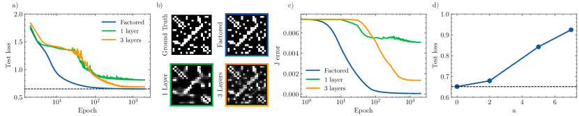
Figure 2: A single layer of factored self-attention learns the generalised Potts model efficiently. (a) Test loss (3) for factored self-attention and for vanilla transformers with one and three layers during training with stochastic gradient descent. The optimal generalisation loss is shown as a black dashed line. (b) Interaction matrix $J$ of the generative Potts Model (1) compared to the attention maps learned by transformers with vanilla and factored self-attention. For the three-layer transformer, the attention map was obtained by averaging the maps of the last two layers. (c) Reconstruction error of the interaction ${(J-A)}^{2}$ as a function of the number of epochs for all considered architectures. (d) Test loss as a function of perturbation level $a$. Decoupling the treatment between positions and colours by decreasing $a$ decreases the test loss. Parameters: sequence length $L=20$, vocabulary size $C=20$, embedding dimension $d=20$, $M=3000$ data points.

We then train off-the-shelf transformers consisting of one and three layers on this data set by minimising the cross-entropy loss between the output distribution and the missing spin using stochastic gradient descent (see supplementary material for the numerical details) on the loss $\mathcal{L}(\mathbf{s})=-L^{-1}\sum_{i=1}^{L}\sum_{\alpha=1}^{C}s_{i\alpha}\log\tilde{p}_{i\alpha}(\mathbf{s})$, for a sequence $\mathbf{s}$. In fig. 2, we show the test loss

$$\epsilon_{g}=\mathbb{E}_{\mathbf{s}\sim P}\left[\mathcal{L}(\mathbf{s})\right]$$ (3)

during training, where $\mathbb{E}\,_{\mathbf{s}\sim P}$ denotes an average over the generative model (1). A transformer with a single layer of self-attention does not attain the optimal generalisation error (black dashed line). By plotting the attention matrix of the single layer, we see that the transformer recovers the original interaction matrix to some degree, albeit not perfectly. Training transformers with three layers on the same data set improves the accuracy at the cost of loosing interpretability: there is no straightforward way to collapse several layers of non-linear transformations of the input sequence into a single attention map; we show the average of the final two attention layers in fig. 2b.

Factored self-attention learns the generalised Potts model.

We now consider a variant of self-attention in which the treatment of positions and values is decoupled. We set $a=0$ in eq. 2 , set the masking token $\mathbf{t}=0$, choose one-hot encodings for the positions, and fix the embedding matrix at $E=I_{C}$, so that

$$h_{i\alpha}\left(\mathbf{s}_{\setminus i}\right)=\sum_{j=1}^{L}A_{ij}(V\mathbf{s}_{j})_{\alpha}$$ (4)

where $A_{ij}\equiv e^{(Q^{\top}K)_{ij}}/\sum_{k=1}^{L}e^{(Q\top K)_{ik}}$. This modified self-attention has exactly the same form as the conditional distribution of the generalised Potts model, which is

$$p(s_{i\alpha}=1|\mathbf{s}_{\setminus i})=\frac{\exp\left({\beta\sum_{j=1}^{L}J_{ij}(U\mathbf{s}_{j})_{\alpha}}\right)}{\sum_{\gamma=1}^{C}\exp\left({\beta\sum_{j=1}^{L}J_{ij}(U\mathbf{s}_{j})_{\gamma}}\right)}.$$ (5)

if one sets $U=V$ and $\beta J~{}=~{}A$. This equivalence between factored self-attention and the Potts model is our first main result; we now discuss its ramifications.

Decoupling positions and colours leads to a significant improvement in the performance of a single layer, which reaches the optimal generalisation error and converges faster, cf. fig. 2a. Factored self-attention recovers the interaction matrix $J$ perfectly, cf. fig. 2b for the attention map and fig. 2c for the reconstruction error of the interaction matrix. In fig. 2d, we show that decoupling the treatment of positions and colours completely performs better than any intermediate solution with $a>0$.

Factored Attention layers, and thus input-independent attention weights, have been already used as a building block for deep transformers, outperforming standard attention in different applications: Bhattacharya et al. (2020) used it to analyse protein sequences and found that a single layer of factored self-attention performed as well as a deep transformer, and significantly better than a single layer of vanilla self-attention, without explicitly explaining this observation. Input-independent and translation-invariant attention weights improved the performance of transformers in computer vision Dai et al. (2021), and using factored attention is key to obtaining state-of-the-art results in approximating ground states of many-body quantum systems Viteritti et al. (2022); Rende et al. (2023); Viteritti et al. (2023).

Intriguingly, MLM with factored self-attention yields exactly the same loss as the pseudo-likelihood method for solving the inverse Ising problem Besag (1975); Cocco and Monasson (2011); Ricci-Tersenghi (2012); Ekeberg et al. (2013); Cocco et al. (2018). The pseudo-likelihood method is statistically consistent Hyvärinen (2006); Ravikumar et al. (2010); Aurell and Ekeberg (2012), i.e. its parameter estimates converge to the true parameters as the number of samples goes to infinity. A direct consequence of the mapping in eq. 4 is thus that MLM with factored self-attention enjoys the same asymptotic optimality.

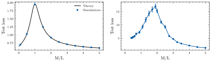
Figure 3: The interpolation peak of factored attention in theory and practice. (Left) A replica analysis predicts the test loss exactly. Test loss of a single layer of factored self-attention as a function of the number of samples per input dimension, as computed using replica theory (solid line). The blue points represent the outcome of numerical minimisation of the square loss (6), averaged over 30 realisations, and show perfect agreement with the theory. Error bars are smaller than point size. (Right) Same plot for a single layer of factored self-attention in the setting of fig. 2 ($L=C=20$), showing the same qualitative behaviour. The simulations are averaged over $n=30$ different realisations.

The sample complexity of self-attention.

A key quantity in machine learning problems is the sample complexity, namely how many samples are required to achieve a small generalisation loss $\epsilon_{g}$ with a given model. The mapping introduced in this work allows addressing this question rigorously for a single layer of self-attention by means of the replica method from statistical physics. The main difficulty in the calculation lies in handling the non-trivial data distribution (1). This difficulty can be mitigated thanks to recent advances in statistical physics, allowing the extension of replica theory to structured data Gerace et al. (2021); Goldt et al. (2022); Loureiro et al. (2022). To perform the replica calculation, we first relax the discrete nature of Potts spins by re-writing the generalised Potts Hamiltonian (1) in terms of spin magnetisation $\mathbf{m}=\langle\mathbf{s}\rangle_{P\left(\mathbf{s}\right)}$ following mean-field theory. The associated Boltzmann measure then turns into a multivariate Gaussian distribution, whose covariance matrix is the negative inverse of the interaction matrix, i.e. $\Sigma=-J^{-1}$ Morcos et al. (2011); Nguyen et al. (2017). We then draw sequences $\{\mathbf{m}^{\mu}\}_{\mu=1}^{M}$ of length $L$ from the multivariate Gaussian with zero mean and covariance matrix $\Sigma=\left(\Omega L^{-1/2}+\nu\mathbb{I}\right)^{-1}$, where $\Omega$ is a symmetric full-rank random matrix sampled from the Gaussian Orthogonal ensemble while $\nu\mathbb{I}$ is a diagonal matrix centering the spectrum of $\Omega$ in $\nu$. To ensure $\Sigma$ to be positive definite, we set $\nu>2$ due to the semicircle law Livan et al. (2018). By fixing the location $i$ of the masked spin across all input sequences, solving the MLM task is equivalent to inferring the $i$th row of the interaction matrix $\mathbf{J}_{i}$.

To accomplish this task, we train a single layer of factored self-attention by empirical risk minimisation of a square loss with $\ell_{2}$-regularisation:

$$\hat{\mathbf{A}}_{i}=\underset{\mathbf{A}_{i}}{\mbox{argmin}}\left[\frac{1}{2}\sum_{\mu=1}^{M}\left(m^{\mu}_{i}-\mathbf{A}_{i}\cdot\mathbf{m}^{\mu}_{\setminus i}\right)^{2}+\frac{\lambda}{2}||\mathbf{A}_{i}||_{2}^{2}\right].$$ (6)

Our goal is to characterise the generalisation loss $\epsilon_{g}$ (3). In the high-dimensional limit, where the number of samples and the sequence length $M,L\rightarrow\infty$ while $\alpha\equiv M/L\sim O\left(1\right)$, we can express $\epsilon_{g}$ using replica theory as a function of only scalar quantities,

$$\epsilon_{g}=\rho+q^{\star}-2r^{\star}+1/\nu.$$ (7)

Here, $\rho=\mbox{tr}\Sigma_{\setminus i}/\left(\nu^{2}L\right)$ is a function of the covariance matrix $\Sigma_{\setminus i}$ where we have removed the $i$th row and column, while $q^{\star}$ and $r^{\star}$ are the so-called overlap parameters. As we show in the supplementary material, the values of these order parameters for a given training set size $\alpha$ can be obtained by solving the optimisation problem

$$f_{\beta}=\underset{q,r,l,\hat{q},\hat{r},\hat{l}}{\mbox{extr}}\left[-\frac{1}{2}\left(\hat{q}l-q\hat{l}\right)+\nu r\hat{r}+\underset{L\rightarrow\infty}{\mbox{lim}}\frac{1}{L}\Psi_{s}+\alpha\Psi_{e}\right]$$ (8)

which yields the typical value (over the data) of the free energy density associated to a Gibbs measure at inverse temperature $\beta$ whose Hamiltonian corresponds to the loss function in eq. 6. Note that the optimisation only involves the scalar parameters $q$, $r$, $l$ and their conjugates  $\hat{q}$, $\hat{r}$ and $\hat{l}$. The entropic and energetic potentials $\Psi_{s}$ and $\Psi_{e}$ are both functions of $\Sigma_{\setminus i}$ and are given in the SM.

We plot the resulting generalisation loss as a function of the rescaled number of samples $\alpha\equiv M/L$ on the right of fig. 3. The test loss actually increases when adding more training sequences to a small data set, before peaking at $\alpha=1$. Below this threshold, the model overfits to its training data; beyond this threshold, the generalisation error decreases monotonically with the training set size; for large $\alpha$, we found $\epsilon_{g}\sim\alpha^{-1/2}$. A similar peak in the generalisation loss has been observed in supervised learning Opper and Kinzel (1996) and it is connected to the well-known “double descent” curve observed in deep neural networks in the presence of label noise Nakkiran et al. (2021). There, the peak is a consequence of overfitting and it appears after an initial decay of the test loss at small $\alpha$. In MLM, we find instead that the peak appears naturally as a consequence of the intrinsic stochasticity of the inputs, which also causes the absence of an initial decay of the loss due to the high level of noise in the labels.

We verify the predictions of the replica theory by plotting the generalisation loss of a single layer of factored self-attention trained on the generalised Potts Model in the setting of fig. 2 at small regularisation (right of fig. 3). We see the same qualitative behaviour as predicted by replica theory, even though in this case we did not apply any of the assumptions required for the replica analysis (the mean field limit, the usage of a full-rank $J$ matrix and of a $U$ matrix fixed to the identity). In particular, the test loss increases when adding more data for small $\alpha$. The only difference between the plots is the location of the peak. For the square loss that we analysed with replicas, it appears at the interpolation threshold, which is the largest number of samples that the neural network can fit perfectly, which is at $M=L$ for a system of linear equations. For the simulations with logistic loss, the peak appears at the linearly separability threshold, which is the largest number of points a linear classifier can classify correctly, and which can be larger than one Gardner and Derrida (1989); Gerace et al. (2021).

Concluding perspectives.

In this work, we have characterised the probability distributions that a single layer of self-attention can learn when trained on the masked language modeling task. In particular, we have shown analytically and numerically that by a single factored-attention layer it is possible to exactly reconstruct the couplings of a generalised Potts model with two-body interactions between both sites and colours. More precisely, we showed that training factored self-attention on the MLM objective is equivalent to solving the inverse Potts problem using the pseudo-likelihood method Besag (1975); Cocco and Monasson (2011); Ricci-Tersenghi (2012); Ekeberg et al. (2013); Cocco et al. (2018), and therefore yields consistent estimators of the parameters. These findings make factored attention a powerful, theoretically-driven building block for deep transformers. Our replica analysis of self-attention enabled us to compute the generalisation loss of the model exactly and yielded a non-trivial generalisation behaviour.

Learning higher-order interactions will require additional layers: a detailed study of how this can be achieved is an interesting direction for future research. It will be interesting to also study the learning dynamics of self-attention using methods from statistical physics Saad and Solla (1995); Biehl and Schwarze (1995); Goldt et al. (2020b); Veiga et al. (2022), both on MLM and on supervised tasks Zhang et al. (2021, 2022); Abbe et al. (2022); Seif et al. (2022). In short, our work clarifies the limits of standard self-attention trained on data where two-body interactions dominate and highlights the potential of factored attention as a component of transformer models.

APPENDIX

Appendix A Numerical details

The numerical simulations were perfomed using JAX Bradbury et al. (2018). Both the factored attention layer and the vanilla transformer architecture were optimised using SGD with mini-batch size of 100 and a cosine annealear as the learning rate decay scheduler, both standard choices in the literature. The initial learning rate was adjusted to the specific simulations, choosing it between 0.1 and 0.01. The vanilla transformer code has been taken from the notebook Lippe (2022), with no modifications made. In particular, as already pointed out in the main text, each element $\mathbf{s}_{i}$ of a sequence $\mathbf{s}=\left(\mathbf{s}_{1},...,\mathbf{s}_{L}\right)$ is first transformed into a token $\mathbf{x}_{i}=\mathbf{e}_{i}+\mathbf{p}_{i}$, with $\mathbf{e}_{i}$ being the embedding of $\mathbf{s}_{i}$ and $\mathbf{p}_{i}$ being the positional encoding. The tokenized sequences are then fed to a layer made of two distinct sub-layers. The first sub-layer is composed of a single-head attention, instead the second sub-layer contains a two layer fully connected neural network. The inputs of both sublayers are connected to their outputs through skip-connections, and layer normalization is then applied.

Finally, there is an output layer consisting of a linear transformation from the $d$- to the $C$-dimensional space, in order to obtain a probability distribution over the colours through the softmax non-linearity. For a graphic visualization of the transformer encoder architecture, reference can be made to the original paper of Vaswani et al. (2017). Below is the list of transformer hyperparameters used for the simulations of fig. 2: embedding dimension 20, number of heads 1, number of layers 1-3, dropout probability 0.0, number of classes 20.

The dataset was generated using Gibbs sampling, starting from a random sequence of $L=20$ sites and $C=20$ Potts colors and cyclically sampling the spins by exploiting the knowledge of the exact conditional probabilities, eq. (5). In order to decorrelate the samples, 10000 Gibbs sweeps were made between each two saved configurations.

The simulations on the left panel of fig. 3, have been performed by sampling the input data-points from a multivariate Gaussian distribution and the masked token from the same distribution, conditioned on the other elements in the sequence. The optimization problem in eq. (6) is then solved in closed-form thanks to the Moore-Penrose inverse as in Gerace et al. (2021).

Appendix B Replica analysis of self-attention

In this section we discuss the replica analysis of a factored single layer self-attention in detail. The computation builds upon the recent advances in statistical physics of learning, concerning the extension of replica theory to structured data Gerace et al. (2021); Goldt et al. (2022); Loureiro et al. (2022). In the following we will show how to slightly modify this new approach in order to deal with masked language modelling tasks, under the following simplified assumptions: mean-field limit, full-rank J matrix, U matrix fixed to the identity and thus not learned.

B.1 Statistical physics formulation of machine learning problems

Statistical physics considers learning as a dynamical and exploratory process across the space of the learnable parameters. At equilibrium, these parameters are assumed to follow a Boltzmann-Gibbs distribution, where the role of the Hamiltonian is actually played by the loss function:

$$\pi_{\beta}\left(\mathbf{A}_{i},\mathcal{D}\right)=\frac{P\left(\mathbf{A}_{i}\right)}{\mathcal{Z}_{\beta}}e^{-\beta\sum_{\mu=1}^{M}\ell\left(m^{\mu}_{i},\frac{\mathbf{A}_{i}\cdot\mathbf{m}^{\mu}_{\setminus i}}{\sqrt{L}}\right)}=\frac{P_{A}\left(\mathbf{A}_{i}\right)}{\mathcal{Z}_{\beta}}\prod_{\mu=1}^{M}P_{G}\left(m^{\mu}_{i}|\frac{\mathbf{A}_{i}\cdot\mathbf{m}^{\mu}_{\setminus i}}{\sqrt{L}}\right)$$ (9)

with $\beta$ being the inverse temperature and $\mathcal{D}$ the training set. In the zero temperature limit (i.e. $\beta\rightarrow\infty$), the Boltzmann-Gibbs distribution concentrates around the minima of the loss function, which are nothing but the solutions of the optimization problem in eq. 6:

$$\hat{\mathbf{A}}_{i}\underset{\beta\rightarrow\infty}{=}\mathbb{E}_{\pi_{\beta}}\left[\mathbf{A}_{i}\right]$$ (10)

Up to this point, re-framing a machine learning problem in terms of statistical physics does not seem to be a great advantage since sampling from an high-dimensional Boltzmann-Gibbs distribution is known to be impracticable.

This is where the replica theory comes into play. In particular, it states that, in the high-dimensional limit (i.e. $M,L\rightarrow\infty$ with $\alpha\equiv M/L\sim O\left(1\right)$) the free-energy of a learning system concentrates around its typical value over the input data distribution:

$$f_{\beta}=-\underset{L\rightarrow\infty}{\mbox{lim}}\frac{1}{L}\mathbb{E}_{\{\mathbf{m}^{\mu}_{\setminus i},m^{\mu}_{i}\}}\left[\mbox{log}\mathcal{Z}_{\beta}\right].$$ (11)

As we will see in the next section, this expectation can be tackled by means of the replica trick. From this quantity, all the high-dimensional metrics of interests, can be computed as a function of simple scalar quantities. This is for instance the case of the generalization loss in eq. (7). In particular, the overlap parameters $m_{\star}$ and $q_{\star}$ correspond to practically measurable quantities over different realisation of the training set, involving the estimator of the $i$th row of the interaction matrix:

$$\begin{split}q^{\star}=\frac{\hat{\mathbf{A}}^{t}_{i}\Sigma_{\setminus i}\hat{\mathbf{A}}_{i}}{L}\hskip 14.22636ptr^{\star}=-\frac{\mathbf{J}_{i}^{t}\Sigma_{\setminus i}\hat{\mathbf{A}}_{i}}{\nu L}.\end{split}$$ (12)

In the next section we will outline the main steps of the replica trick leading to the generalization loss formula in eq. (7).

B.2 Replica Calculation

As anticipated in the previous section, the replica trick allows to compute the typical value of the free-energy density in eq. (11) by expressing this quantity as a function of the solely replicated partition function $\mathcal{Z}_{\beta}^{n}$, obtained by constructing $n>0$ different and independent copies of the same learning system:

$$f_{\beta}=-\underset{n\rightarrow 0^{+}}{\mbox{lim}}\frac{d}{dn}\underset{L\rightarrow\infty}{\mbox{lim}}\left[\frac{1}{L}\mathbb{E}_{\{\mathbf{m}^{\mu}_{\setminus i},m^{\mu}_{i}\}}\mathcal{Z}_{\beta}^{n}\right].$$ (13)

Average over the training set.

As a first step, the replica calculation focuses on the expectation of the replicated partition function over the training set, which, written in a more explicit form, looks like:

$$\mathbb{E}_{\{\mathbf{m}^{\mu}_{\setminus i},m^{\mu}_{i}\}}\mathcal{Z}^{n}_{\beta}=\mathbb{E}_{\{m^{\mu}_{i}|\mathbf{m}^{\mu}_{\setminus i}\}}\mathbb{E}_{\mathbf{m}^{\mu}_{\setminus i}}\left[\int\prod_{a=1}^{n}d\mathbf{A}_{i}^{a}\prod_{a=1}^{n}\ P_{A}\left(\mathbf{A}_{i}^{a}\right)\prod_{\mu=1}^{M}P_{G}\left(m_{i}^{\mu}\mid\frac{\mathbf{A}^{a}_{i}\cdot\mathbf{m}^{\mu}_{\setminus i}}{\sqrt{L}}\right)\right],$$ (14)

with $P_{G}$ and $P_{A}$ being respectively the Gibbs and the Gaussian measure associated to the $i$th row of the attention matrix as in eq. (9). Indeed, as already pointed out in the main manuscript, the interaction matrix is drawn from the Gaussian Orthogonal Ensemble, therefore its rows will correspond to Gaussian random vectors. At this point, we can notice an important aspect of MLM tasks. In this case, the labels are not provided by a teacher vector as in standard teacher-student settings. On the contrary, the masked tokens are directly sampled from the input distribution by conditioning over all the other elements composing the sequence:

$$m_{i}^{\mu}\sim\frac{P_{J}\left(\mathbf{J}_{i}\right)}{\sqrt{2\pi\nu^{-1}}}e^{-\frac{1}{2\nu^{-1}}\left(m^{\mu}_{i}+\frac{\mathbf{J}_{i}\cdot\mathbf{m}^{\mu}_{\setminus i}}{\nu\sqrt{L}}\right)^{2}}=P_{J}\left(\mathbf{J}_{i}\right)P_{0}\left(m_{i}^{\mu}\mid\frac{\mathbf{J}_{i}\cdot\mathbf{m}^{\mu}_{\setminus i}}{\nu\sqrt{L}}\right).$$ (15)

Note that, the noise in the labels arises a consequence of the one already affecting the input data points, meaning that its intensity can not be chosen independently from the intrinsic stochasticity of the input. Due to these considerations, by explicitly expressing the outer expectation in eq. (14), we then get:

$$\begin{split}\mathbb{E}_{\{\mathbf{m}^{\mu}_{\setminus i},m^{\mu}_{i}\}}\mathcal{Z}^{n}_{\beta}&=\int d\mathbf{J}_{i}\ P_{J}\left(\mathbf{J}_{i}\right)\int\prod_{a=1}^{n}d\mathbf{A}_{i}^{a}\prod_{a=1}^{n}\ P_{A}\left(\mathbf{A}_{i}^{a}\right)\times\\ &\times\int dm_{i}^{\mu}\ \mathbb{E}_{\mathbf{m}^{\mu}_{\setminus i}}\left[\prod_{\mu=1}^{M}P_{0}\left(m_{i}^{\mu}\mid\frac{\mathbf{J}_{i}\cdot\mathbf{m}^{\mu}_{\setminus i}}{\nu\sqrt{L}}\right)P_{G}\left(m_{i}^{\mu}\mid\frac{\mathbf{A}^{a}_{i}\cdot\mathbf{m}^{\mu}_{\setminus i}}{\sqrt{L}}\right)\right].\end{split}$$ (16)

To compute the expectation over the input sequences with a masked element at position $i$, we first define the pre-activations as:

$$h^{\mu}_{a}=\frac{\mathbf{A}^{a}_{i}\cdot\mathbf{m}^{\mu}_{\setminus i}}{\sqrt{L}}\hskip 28.45274ptz^{\mu}=-\frac{\mathbf{J}_{i}\cdot\mathbf{m}^{\mu}_{\setminus i}}{\nu\sqrt{L}},$$ (17)

then we express these definitions in terms of Dirac-deltas and their corresponding integral representation:

$$\begin{split}&1\propto\int\prod_{\mu=1}^{M}\prod_{a=1}^{n}dh_{a}^{\mu}\ \delta\left(h_{a}^{\mu}-\frac{\mathbf{A}^{a}_{i}\cdot\mathbf{m}^{\mu}_{\setminus i}}{\sqrt{L}}\right)=\int\prod_{\mu=1}^{M}\prod_{a=1}^{n}\frac{dh_{a}^{\mu}d\hat{h}^{\mu}_{a}}{2\pi}\prod_{\mu=1}^{M}e^{i\hat{h}^{\mu}_{a}\left(h_{a}^{\mu}-\frac{\mathbf{A}^{a}_{i}\cdot\mathbf{m}^{\mu}_{\setminus i}}{\sqrt{L}}\right)}\\ &1\propto\int\prod_{\mu=1}^{M}dz^{\mu}\ \delta\left(z^{\mu}+\frac{\mathbf{J}_{i}\cdot\mathbf{m}^{\mu}_{\setminus i}}{\nu\sqrt{L}}\right)=\int\prod_{\mu=1}^{M}\frac{dz^{\mu}d\hat{z}^{\mu}}{2\pi}\prod_{\mu=1}^{M}\ e^{i\hat{z}^{\mu}\left(z^{\mu}+\frac{\mathbf{J}_{i}\cdot\mathbf{m}^{\mu}_{\setminus i}}{\nu\sqrt{L}}\right)}.\end{split}$$ (18)

By plugging these factors one into eq. (16), we then get:

$$\begin{split}\mathbb{E}_{\{\mathbf{m}^{\mu}_{\setminus i},m^{\mu}_{i}\}}\mathcal{Z}^{n}_{\beta}&=\int d\mathbf{J}_{i}\ P_{J}\left(\mathbf{J}_{i}\right)\int\prod_{a=1}^{n}d\mathbf{A}_{i}^{a}\ \prod_{a=1}^{n}P_{A}\left(\mathbf{A}_{i}^{a}\right)\times\\ &\times\int\prod_{\mu=1}^{M}dm_{i}^{\mu}\int\prod_{\mu=1}^{M}\frac{dz^{\mu}d\hat{z}^{\mu}}{2\pi}\prod_{\mu=1}^{M}e^{i\hat{z}^{\mu}z^{\mu}}\prod_{\mu=1}^{M}P_{0}\left(m_{i}^{\mu}\mid z^{\mu}\right)\times\\ &\times\int\prod_{\mu=1}^{M}\prod_{a=1}^{n}\frac{dh_{a}^{\mu}d\hat{h}_{a}^{\mu}}{2\pi}\prod_{\mu=1}^{M}\prod_{a=1}^{n}e^{i\hat{h}_{a}^{\mu}h_{a}^{\mu}}\prod_{\mu=1}^{M}\prod_{a=1}^{n}P_{G}\left(m_{i}^{\mu}\mid h_{a}^{\mu}\right)\times\\ &\times\prod_{\mu=1}^{n}\mathbb{E}_{\mathbf{m}^{\mu}_{\setminus i}}\left[e^{i\hat{z}^{\mu}\frac{\mathbf{J}_{i}\cdot\mathbf{m}^{\mu}_{\setminus i}}{\nu\sqrt{L}}}\prod_{a=1}^{n}e^{-i\hat{h}_{a}^{\mu}\frac{\mathbf{A}^{a}_{i}\cdot\mathbf{m}^{\mu}_{\setminus i}}{\sqrt{L}}}\right].\end{split}$$ (19)

The expectation over the masked input sequences is a simple multivariate Gaussian integral, whose solution is given by:

$$\begin{split}\mathbb{E}_{\mathbf{m}^{\mu}_{\setminus i}}\left[e^{i\hat{z}^{\mu}\frac{\mathbf{J}_{i}\cdot\mathbf{m}^{\mu}_{\setminus i}}{\nu\sqrt{L}}}\prod_{a=1}^{n}e^{-i\hat{h}_{a}^{\mu}\frac{\mathbf{A}^{a}_{i}\cdot\mathbf{m}^{\mu}_{\setminus i}}{\sqrt{L}}}\right]=e^{-\frac{1}{2}\frac{\mathbf{J}_{i}^{t}\Sigma_{\setminus i}\mathbf{J}_{i}}{\nu^{2}L}\left(z^{\mu}\right)^{2}+\sum_{a=1}^{n}\frac{\mathbf{J}_{i}^{t}\Sigma_{\setminus i}\mathbf{A}_{i}^{a}}{\nu L}\hat{h}^{\mu}_{a}\hat{z}^{\mu}-\frac{1}{2}\sum_{a,b=1}^{n}\frac{\left(\mathbf{A}_{i}^{a}\right)^{t}\Sigma_{\setminus i}\mathbf{A}_{i}^{a}}{L}\hat{h}^{\mu}_{a}\hat{h}^{\mu}_{b}}\end{split}$$ (20)

where, as already pointed out in the main text, $\Sigma_{\setminus i}$ corresponds to the covariance matrix of the masked input sequences, that is the input covariance matrix without the contribution of the row and column associated to the $i$th masked token. By replacing the solution of the expectation in eq. (19), we then get:

$$\begin{split}\mathbb{E}_{\{\mathbf{m}^{\mu}_{\setminus i},m^{\mu}_{i}\}}\mathcal{Z}^{n}_{\beta}&=\int d\mathbf{J}_{i}\ P_{J}\left(\mathbf{J}_{i}\right)\int\prod_{a=1}^{n}d\mathbf{A}_{i}^{a}\ \prod_{a=1}^{n}P_{A}\left(\mathbf{A}_{i}^{a}\right)\times\\ &\times\int\prod_{\mu=1}^{M}dm_{i}^{\mu}\int\prod_{\mu=1}^{M}\frac{dz^{\mu}d\hat{z}^{\mu}}{2\pi}\prod_{\mu=1}^{M}e^{i\hat{z}^{\mu}z^{\mu}}\prod_{\mu=1}^{M}P_{0}\left(m_{i}^{\mu}\mid z^{\mu}\right)\times\\ &\times\int\prod_{\mu=1}^{M}\prod_{a=1}^{n}\frac{dh_{a}^{\mu}d\hat{h}_{a}^{\mu}}{2\pi}\prod_{\mu=1}^{M}\prod_{a=1}^{n}e^{i\hat{h}_{a}^{\mu}h_{a}^{\mu}}\prod_{\mu=1}^{M}\prod_{a=1}^{n}P_{G}\left(m_{i}^{\mu}\mid h_{a}^{\mu}\right)\times\\ &\times\prod_{\mu=1}^{n}e^{-\frac{1}{2}\frac{\mathbf{J}_{i}^{t}\Sigma_{\setminus i}\mathbf{J}_{i}}{\nu^{2}L}\left(z^{\mu}\right)^{2}+\sum_{a=1}^{n}\frac{\mathbf{J}_{i}^{t}\Sigma_{\setminus i}\mathbf{A}_{i}^{a}}{\nu L}\hat{h}^{\mu}_{a}\hat{z}^{\mu}-\frac{1}{2}\sum_{a,b=1}^{n}\frac{\left(\mathbf{A}_{i}^{a}\right)^{t}\Sigma_{\setminus i}\mathbf{A}_{i}^{a}}{L}\hat{h}^{\mu}_{a}\hat{h}^{\mu}_{b}}.\end{split}$$ (21)

Rewriting the averaged replicated partition function in terms of saddle-point integrals.

As a consequence of the average over the training set, the different replicas are now interacting among each other through the following set of overlap parameters:

$$\rho=\frac{\mathbf{J}_{i}^{t}\Sigma_{\setminus i}\mathbf{J}_{i}}{\nu^{2}L}\hskip 28.45274ptr_{a}=-\frac{\left(\mathbf{A}_{i}^{a}\right)^{t}\Sigma_{\setminus i}\mathbf{J}_{i}}{\nu L}\hskip 28.45274ptq_{ab}=-\frac{\left(\mathbf{A}_{i}^{a}\right)^{t}\Sigma_{\setminus i}\mathbf{A}_{i}^{b}}{L}.$$ (22)

Once again, to proceed further in the calculation, we can insert their definition by means of Dirac-deltas and their integral representation:

$$\begin{split}&1\propto\int d\rho\ \delta\left(\nu^{2}L\rho-\mathbf{J}_{i}^{t}\Sigma_{\setminus i}\mathbf{J}_{i}\right)=\int\frac{d\rho d\hat{\rho}}{2\pi}\ e^{i\hat{\rho}\left(\nu^{2}L\rho-\mathbf{J}_{i}^{t}\Sigma_{\setminus i}\mathbf{J}_{i}\right)}\\ &1\propto\int\prod_{a=1}^{n}dr_{a}\ \delta\left(-\nu Lr_{a}-\left(\mathbf{A}^{a}_{i}\right)^{t}\Sigma_{\setminus i}\mathbf{J}_{i}\right)=\int\prod_{a=1}^{n}\frac{dr_{a}d\hat{r}_{a}}{2\pi}\prod_{a=1}^{n}\ e^{i\hat{r}_{a}\left(-\nu Lr_{a}-\left(\mathbf{A}^{a}_{i}\right)^{t}\Sigma_{\setminus i}\mathbf{J}_{i}\right)}\\ &1\propto\int\prod_{a\leq b}dq_{ab}\ \delta\left(Lq_{ab}-\left(\mathbf{A}^{a}_{i}\right)^{t}\Sigma_{\setminus i}\mathbf{A}^{b}_{i}\right)=\int\prod_{a\leq b}\frac{dq_{ab}d\hat{q}_{ab}}{2\pi}\prod_{a\leq b}\ e^{i\hat{q}_{ab}\left(q_{ab}-\left(\mathbf{A}^{a}_{i}\right)^{t}\Sigma_{\setminus i}\mathbf{A}^{b}_{i}\right)}.\end{split}$$ (23)

By substituting the overlap definition in eq. (21), plugging in the corresponding factors one and performing the change of variables: $i\hat{\rho}\rightarrow-\hat{\rho}$, $i\hat{r}_{a}\rightarrow\hat{r}_{a}$ and $i\hat{q}_{ab}\rightarrow\hat{q}_{ab}$, we can rewrite the averaged replicated partition function in terms of saddle-point integrals over the overlap parameters:

$$\mathbb{E}_{\{\mathbf{m}^{\mu}_{\setminus i},m^{\mu}_{i}\}}\mathcal{Z}^{n}_{\beta}=\int\frac{d\rho d\hat{\rho}}{2\pi}\int\prod_{a=1}^{n}\frac{dr_{a}d\hat{r}_{a}}{2\pi}\int\prod_{a\leq b}\frac{dq_{ab}d\hat{q}_{ab}}{2\pi}\ e^{L\Psi^{\left(n\right)}}$$ (24)

where the action $\Psi^{\left(n\right)}$ is a non trivial function of the overlap parameters:

$$\Psi^{\left(n\right)}=-\nu^{2}\rho\hat{\rho}+\nu\sum_{a=1}^{n}r_{a}\hat{r}_{a}-\sum_{a\leq b}q_{ab}\hat{q}_{ab}+\frac{1}{L}\Psi_{s}+\frac{M}{L}\Psi_{e}$$ (25)

where $\Psi_{s}$ and $\Psi_{e}$ are the so-called entropic and energetic potential and, in the specific case of a single-layer factored attention, are given by:

$$\begin{split}\Psi_{s}&=\mbox{log}\left[\int d\mathbf{J}_{i}P_{J}\left(\mathbf{J}_{i}\right)\int\prod_{a=1}^{n}d\mathbf{A}_{i}^{a}P_{A}\left(\mathbf{A}_{i}^{a}\right)e^{\hat{\rho}\mathbf{J}_{i}^{t}\Sigma_{\setminus i}\mathbf{J}_{i}+\sum_{a=1}^{n}\hat{r}_{a}\left(\mathbf{A}_{i}^{a}\right)^{t}\Sigma_{\setminus i}\mathbf{J}_{i}+\sum_{a\leq b}\hat{q}_{ab}\left(\mathbf{A}_{i}^{a}\right)^{t}\Sigma_{\setminus i}\mathbf{A}_{i}^{b}}\right]\\ \Psi_{e}&=\mbox{log}\left[\int dm_{i}\int\frac{dzd\hat{z}}{2\pi}\ e^{-\frac{\rho}{2}\hat{z}^{2}+i\hat{z}z}P_{0}\left(m_{i}|z\right)\right.\times\\ &\left.\times\int\prod_{a=1}^{n}\frac{dh_{a}d\hat{h}_{a}}{2\pi}\ e^{-\frac{1}{2}\sum_{a,b=1}^{n}q_{ab}\hat{h}_{a}\hat{h}_{b}-\hat{z}\sum_{a=1}^{n}r_{a}\hat{h}_{a}+i\sum_{a=1}^{n}\hat{h}_{a}h_{a}}P_{G}\left(m_{i}|h_{a}\right)\right].\end{split}$$ (26)

Note that, we have drop the dependency of $\Psi_{e}$ on the $\mu$ index since all the $\mu$-dependent terms decouple with respect to $\mu$.

Replica Symmetric Assumption.

To proceed further in the calculation, we need to assume a specific replica structure. Since all replicas have been introduced independently from each other with no specific differences among them, it seems natural to assume that replicas should all play the same role and that, therefore, the overlap parameters should not depend on the specific replica index. In particular, under the replica symmetric ansatz, we assume:

$$\begin{split}q_{ab}&=\begin{cases}g&\text{if}\ a=b\\ q&\text{otherwise}\end{cases}\hskip 42.67912pt-i\hat{q}_{ab}=\begin{cases}-\frac{\hat{g}}{2}&\text{if}\ a=b\\ \hat{q}&\text{otherwise}\end{cases}\\ \\ r_{a}&=r\hskip 28.45274pt\hskip 79.66771pt-i\hat{r}_{a}=\hat{r}\hskip 14.22636pt\forall a\\ \end{split}$$ (27)

By plugging the replica symmetric assumption in eq. (25)-(29) we get the following expression for the action:

$$\Psi^{\left(n\right)}=-\nu^{2}\rho\hat{\rho}+\nu r\hat{r}+\frac{n}{2}\left(l+q\right)\left(\hat{l}-\hat{q}\right)-\frac{n\left(n-1\right)}{2}q\hat{q}+\frac{1}{L}\Psi_{s}+\frac{M}{L}\Psi_{e}$$ (28)

where the replica symmetric potentials $\Psi_{s}$ and $\Psi_{e}$ are are given by:

$$\begin{split}\Psi_{s}&=\mbox{log}\left[\int d\mathbf{J}_{i}P_{J}\left(\mathbf{J}_{i}\right)e^{\hat{\rho}\mathbf{J}_{i}^{t}\Sigma_{\setminus i}\mathbf{J}_{i}}\right.\times\\ &\left.\times\int\prod_{a=1}^{n}d\mathbf{A}_{i}^{a}P_{A}\left(\mathbf{A}_{i}^{a}\right)e^{\hat{r}\sum_{a=1}^{n}\left(\mathbf{A}_{i}^{a}\right)^{t}\Sigma_{\setminus i}\mathbf{J}_{i}-\frac{\hat{l}}{2}\sum_{a=1}^{n}\left(\mathbf{A}_{i}^{a}\right)^{t}\Sigma_{\setminus i}\mathbf{A}_{i}^{a}+\frac{\hat{q}}{2}\sum_{a\leq b}\left(\mathbf{A}_{i}^{a}\right)^{t}\Sigma_{\setminus i}\mathbf{A}_{i}^{b}}\right]\\ \Psi_{e}&=\mbox{log}\left[\int dm_{i}\int\frac{dzd\hat{z}}{2\pi}\ e^{-\frac{\rho}{2}\hat{z}^{2}+i\hat{z}z}P_{0}\left(m_{i}|z\right)\right.\times\\ &\left.\times\int\prod_{a=1}^{n}\frac{dh_{a}d\hat{h}_{a}}{2\pi}\ e^{-\frac{q}{2}\sum_{a,b=1}^{n}\hat{h}_{a}\hat{h}_{b}-\frac{l}{2}\sum_{a=1}^{n}\hat{h}^{2}_{a}-r\hat{z}\sum_{a=1}^{n}\hat{h}_{a}+i\sum_{a=1}^{n}\hat{h}_{a}h_{a}}P_{G}\left(m_{i}|h_{a}\right)\right].\end{split}$$ (29)

where we have defined $\hat{l}=\hat{g}+\hat{q}$ and $l=g-q$. To factorise over the replica index, we can apply the Hubbard-Stratonovich transformations

$$\begin{split}e^{\frac{\hat{q}}{2}\sum_{a\leq b}\left(\mathbf{A}^{a}\right)^{t}\Sigma_{\setminus i}\mathbf{A}^{b}}&=\int\mathcal{D}\bm{\xi}\ \mbox{exp}\left(\sum_{a=1}^{n}\left(\mathbf{A}_{i}^{a}\right)^{t}\left(\hat{q}\Sigma_{\setminus i}\right)^{1/2}\bm{\xi}\right)\\ e^{-\frac{q}{2}\sum_{a,b=1}^{n}\hat{h}_{a}\hat{h}_{b}}&=\int\mathcal{D}\xi\ \mbox{exp}\left(i\sqrt{q}\sum_{a=1}^{n}\hat{h}^{2}_{a}\ \xi\right),\end{split}$$ (30)

with $\xi\sim\mathcal{N}\left(0,1\right)$, on both the entropic and energetic potential, thus getting:

$$\begin{split}\Psi_{s}&=\mbox{log}\left[\int d\mathbf{J}_{i}P_{J}\left(\mathbf{J}_{i}\right)e^{\hat{\rho}\mathbf{J}_{i}^{t}\Sigma_{\setminus i}\mathbf{J}_{i}}\int\mathcal{D}\bm{\xi}\left(\int d\mathbf{A}_{i}P_{A}\left(\mathbf{A}_{i}\right)e^{\hat{r}\mathbf{A}_{i}^{t}\Sigma_{\setminus i}\mathbf{J}_{i}-\frac{\hat{l}}{2}\mathbf{A}_{i}^{t}\Sigma_{\setminus i}\mathbf{A}_{i}+\mathbf{A}^{t}_{i}\left(\hat{q}\Sigma_{\setminus i}\right)^{1/2}\bm{\xi}}\right)^{n}\right]\\ \Psi_{e}&=\mbox{log}\left[\int dm_{i}\int\frac{dzd\hat{z}}{2\pi}\ e^{-\frac{\rho}{2}\hat{z}^{2}+i\hat{z}z}P_{0}\left(m_{i}|z\right)\int\mathcal{D}\xi\left(\int\frac{dhd\hat{h}}{2\pi}\ e^{-\frac{l}{2}\hat{h}^{2}+i\sqrt{q}\xi\hat{h}-m\hat{z}\hat{h}+i\hat{h}h}P_{G}\left(m_{i}|h\right)\right)^{n}\right]\end{split}$$ (31)

Zero Replica limit.

By taking the limit of $n\rightarrow 0$ in eq. (28)-(31) and solving the integrals with respect to the $\hat{z}$ and $\hat{h}$ variables, we then get the following expression for the action potential:

$$\Psi^{\left(n\rightarrow 0\right)}=\nu r\hat{r}+\frac{1}{2}\left(l+q\right)\left(\hat{l}-\hat{q}\right)+\frac{1}{2}q\hat{q}+\frac{1}{L}\Psi_{s}^{\left(n\rightarrow 0\right)}+\frac{M}{L}\Psi_{e}^{\left(n\rightarrow 0\right)}$$ (32)

with the entropic and energetic potentials in the zero replicas limit given by:

$$\begin{split}\Psi_{s}^{\left(n\rightarrow 0\right)}&=\int\mathcal{D}\bm{\xi}\int d\mathbf{J}_{i}P_{J}\left(\mathbf{J}_{i}\right)\mbox{log}\left[\int d\mathbf{A}_{i}P_{A}\left(\mathbf{A}_{i}\right)e^{\hat{r}\mathbf{A}_{i}^{t}\Sigma_{\setminus i}\mathbf{J}_{i}-\frac{\hat{l}}{2}\mathbf{A}_{i}^{t}\Sigma_{\setminus i}\mathbf{A}_{i}+\mathbf{A}^{t}_{i}\left(\hat{q}\Sigma_{\setminus i}\right)^{1/2}\bm{\xi}}\right]\\ \Psi_{e}^{\left(n\rightarrow 0\right)}&=\int\mathcal{D}\xi\int dm_{i}\int\frac{dz}{\sqrt{2\pi\left(\rho-\frac{r^{2}}{q}\right)}}\ e^{-\frac{\left(z+\frac{r}{\sqrt{q}}\xi\right)^{2}}{2\left(\rho-\frac{r^{2}}{q}\right)}}P_{0}\left(m_{i}|z\right)\mbox{log}\left[\int\frac{dh}{\sqrt{2\pi l}}\ e^{-\frac{\left(h+\sqrt{q}\xi\right)^{2}}{2l}}P_{G}\left(m_{i}|h\right)\right]\end{split}$$ (33)

Note that, as in standard teacher-student settings Gerace et al. (2021), in order to avoid divergent terms in this limit, the overlap $\rho$ and its conjugate $\hat{\rho}$ need to be constrained to $\mathbb{E}_{\mathbf{J}_{i}}\left[\mathbf{J}_{i}^{t}\Sigma_{\setminus i}\mathbf{J}_{i}\right]/\nu^{2}$ and $0$ respectively.

Typical Free-Energy density.

Having determined the expression for the replicated partition function in the zero-temperature limit, we can actually compute the typical free-energy density as:

$$f_{\beta}=-\underset{n\rightarrow 0^{+}}{\mbox{lim}}\frac{d}{dn}\underset{L\rightarrow\infty}{\mbox{lim}}\left[\frac{1}{L}\mathbb{E}_{\{\mathbf{m}^{\mu}_{\setminus i},m^{\mu}_{i}\}}\mathcal{Z}_{\beta}^{n}\right]=\underset{L\rightarrow\infty}{\mbox{lim}}\frac{1}{L}\int\frac{d\rho d\hat{\rho}}{2\pi}\int\frac{drd\hat{r}}{2\pi}\int\frac{dqd\hat{q}}{2\pi}\ e^{L\Psi^{\left(n\rightarrow 0\right)}}.$$ (34)

In the high-dimensional limit, we can solve the integrals over the overlap parameters by saddle-point, thus getting:

$$f_{\beta}=\underset{q,r,l,\hat{q},\hat{r},\hat{l}}{\mbox{extr}}\left[\nu r\hat{r}+\frac{1}{2}\left(l+q\right)\left(\hat{l}-\hat{q}\right)+\frac{1}{2}q\hat{q}+\underset{L\rightarrow\infty}{\mbox{lim}}\frac{1}{L}\Psi_{s}^{\left(n\rightarrow 0\right)}+\alpha\Psi_{e}^{\left(n\rightarrow 0\right)}\right].$$ (35)

where the values of the overlap parameters extremizing the typical free-energy density can therefore be determined by solving the following system of coupled saddle-point equations:

$$\begin{split}\begin{cases}q=-2\frac{\partial\Psi_{s}^{\left(n\rightarrow 0\right)}}{\partial\hat{l}}\\ l=2\frac{\partial\Psi_{s}^{\left(n\rightarrow 0\right)}}{\partial\hat{q}}\\ r=-\frac{1}{\nu}\frac{\partial\Psi_{s}^{\left(n\rightarrow 0\right)}}{\partial\hat{r}}\end{cases}\hskip 42.67912pt\begin{cases}\hat{q}=2\frac{\partial\Psi_{e}^{\left(n\rightarrow 0\right)}}{\partial l}\\ \hat{l}=-2\frac{\partial\Psi_{e}^{\left(n\rightarrow 0\right)}}{\partial q}\\ \hat{r}=-\frac{1}{\nu}\frac{\partial\Psi_{e}^{\left(n\rightarrow 0\right)}}{\partial r}\end{cases}\\ \\ \end{split}$$ (36)

Up to this point, we have performed the replica calculation in full generality, without specifying neither the interaction matrix nor the loss function. In the next section, we will evaluate the typical free-energy density for the specific MLM task of eq. (6) under the simplified assumptions of the sec. The sample complexity of self-attention of the main text.

Zero temperature limit and Gaussian Priors.

As already pointed out in the main text, the interaction matrix $J$ is sampled from the GOE, it is then natural to assume a Gaussian prior on the $i$th row of the attention matrix:

$$P_{A}\left(\mathbf{\mathbf{A}}\right)=\frac{1}{\sqrt{2\pi}}e^{\beta\lambda\mathbf{A}_{i}^{t}\mathbf{A}_{i}}$$ (37)

with $\beta$ being the inverse temperature parameter, while $\lambda$ being the $L_{2}$ regularization strength. Moreover, the optimization problem in eq. (6) optimize a square loss to solve the corresponding MLM task. This means that, the Gibbs Measure of eq. (9) associated to this task is:

$$P_{G}\left(m_{i}|h\right)\propto e^{-\frac{\beta}{2}\left(m_{i}-h\right)^{2}}.$$ (38)

By plugging these two specific forms of both the prior and the Gibbs measure in eq. (14) and taking the zero temperature limit as exemplified in Gerace et al. (2021); Goldt et al. (2022), we get the following expression for the typical free-energy density in the zero-temperature limit:

$$f\underset{\beta\rightarrow\infty}{=}\underset{q,r,l,\hat{q},\hat{r},\hat{l}}{\mbox{extr}}\left[\nu r\hat{r}-\frac{1}{2}\left(l\hat{q}-q\hat{l}\right)+\underset{L\rightarrow\infty}{\mbox{lim}}\frac{1}{L}\Psi_{s}^{\left(n\rightarrow 0\right)}+\alpha\Psi_{e}^{\left(n\rightarrow 0\right)}\right].$$ (39)

with the entropic and energetic potential given by:

$$\begin{split}\Psi_{s}^{n\rightarrow 0}&\underset{\beta\rightarrow\infty}{=}\frac{1}{2}\left[\hat{r}^{2}\mbox{tr}\left(\Sigma_{\setminus i}\right)^{t}\Sigma_{\setminus i}\left(\beta\lambda\mathbb{I}+\hat{l}\Sigma_{\setminus i}\right)^{-1}+\hat{q}\mbox{tr}\Sigma_{\setminus i}\left(\beta\lambda\mathbb{I}+\hat{l}\Sigma_{\setminus i}\right)^{-1}\right]\\ \Psi_{e}^{n\rightarrow 0}&\underset{\beta\rightarrow\infty}{=}-\frac{1}{2}\frac{\nu^{-1}+\rho+q-2r}{1+l}\end{split}$$ (40)

and $\rho=\mbox{tr}\Sigma_{\setminus i}/\left(\nu^{2}L\right)$. Note that, this functional form of the typical free-energy density corresponds exactly to the one of supervised learning with noisy label and Gaussian structured data Goldt et al. (2022). However, we should here point out again that, the variance of the noise in the labels, controlled by the shift factor $\nu$, is a direct consequence of the intrinsic noise already affecting the input. Therefore, it can not be tuned independently from it. This is also reflected on the slightly different functional form of the saddle-point equations in (36), which, in the zero-temperature limit with Gaussian priors and square loss, are given by:

$$\begin{split}\begin{cases}q=\mbox{tr}\left[\left(\hat{q}\Sigma_{\setminus i}+\hat{r}^{2}\Sigma_{\setminus i}\left(\Sigma_{\setminus i}\right)^{t}\right)\Sigma_{\setminus i}\left(\lambda\mathbb{I}+\hat{l}\Sigma_{\setminus i}\right)^{-2}\right]\\ l=\mbox{tr}\left[\left(\lambda\mathbb{I}+\hat{l}\Sigma_{\setminus i}\right)^{-1}\Sigma_{\setminus i}\right]\\ r=-\frac{\hat{r}}{\nu}\mbox{tr}\left[\Sigma_{\setminus i}\left(\Sigma_{\setminus i}\right)^{t}\left(\lambda\mathbb{I}+\hat{l}\Sigma_{\setminus i}\right)^{-1}\right]\end{cases}\hskip 42.67912pt\begin{cases}\hat{q}=\frac{\nu^{-1}+\rho+q-2r}{\left(1+l\right)^{2}}\\ \hat{l}=\frac{1}{1+l}\\ \hat{r}=-\frac{1}{\nu\left(1+l\right)}\end{cases}.\\ \\ \end{split}$$ (41)

As in the case of supervised learning settings Gerace et al. (2021); Goldt et al. (2022), the solution of this system of coupled saddle-point equations in the zero temperature limit allows to express the generalization loss as shown in eq. of the main text, with the exception that the noise in the labels is the direct consequence of the intrinsic noise of the inputs.