Radio Galaxy Zoo EMU: Towards a Semantic Radio Galaxy Morphology Taxonomy

Abstract

We present a novel natural language processing (NLP) approach to deriving plain English descriptors for science cases otherwise restricted by obfuscating technical terminology. We address the limitations of common radio galaxy morphology classifications by applying this approach. We experimentally derive a set of semantic tags for the Radio Galaxy Zoo EMU (Evolutionary Map of the Universe) project and the wider astronomical community. We collect 8,486 plain English annotations of radio galaxy morphology, from which we derive a taxonomy of tags. The tags are plain English. The result is an extensible framework which is more flexible, more easily communicated, and more sensitive to rare feature combinations which are indescribable using the current framework of radio astronomy classifications.

1 Introduction

Language is often difficult to define or use. When new concepts arise and demand their own terminology, terms can be adopted from similar ideas (e. g. ‘entropy’ in information theory and physics; Natal et al., 2021), invented (e. g. ‘utopia’; Romm, 1991), or named after the discoverers (e. g. ‘Newtonian physics’). Individual terms often have multiple accepted definitions within a given field, and especially across fields (e. g. ‘modern’ in philosophy and art; Schelling, 1994; Adajian, 2022). The construction of language in science is especially important, as language is believed to affect how we think (Wolff & Holmes, 2010).

The terminology used in astronomy struggles with these same issues. Some terms are obfuscated, poorly defined, or so specific that experts can often only engage in the subject matter if a definition is provided on each use. In radio astronomy, a field which began in the 1930s (Southworth, 1956), the language used to describe celestial objects has been developed almost entirely in tandem with the instruments and corresponding scientific understanding. Consequently, some terms are limited by our physical understanding (e. g. Little Green Man 1; Hewish et al., 1968) or the sample inspected at the time (e. g. FRI / FRII; Fanaroff & Riley, 1974).

In the case of radio galaxy morphologies, language is becoming increasingly difficult to use, especially as technological and scientific advancements provide deeper insight into the vast range of radio morphologies. The gap between the diverse range of observed radio galaxy morphologies and the classification schemes used is widening. The current morphological classifications carry information which cannot be quantified under current frameworks, meaning the use of non-numeric features, i. e. language based schemes, is unavoidable. Accordingly, the current classification schemes fall victim to obfuscated language. Additionally, the terms used tend to describe abstract classes, which lack the ability to capture the increasingly complex features of radio galaxies observed with the newest generation of instruments. Rudnick (2021) urges the radio astronomy community to develop a tagging system rather than forcibly attempting to create classes which neatly separate objects. Such a tagging system would allow an object to be assigned plain English descriptors capturing the semantics of the object’s features through tags rather than be assigned a distinct class to which it belongs. Additionally, this tagging system would be able to consolidate instrument specific morphologies within the same framework without producing conflicts. As an example, a source could be tagged as ‘compact’ in a low resolution survey while having specific morphological features captured by tags referring to observations made by higher resolution instruments. This work aims to build the framework for such a tagging system for the first time.

The newest radio instruments in operation are producing maps of sources which are so deep, resolved, and with such high dynamic range that our existing classification schemes are failing. An updated, and extensible, radio morphology taxonomy of tags would be a tremendous benefit moving forward because deeper and wider surveys are expected to be a massive driver of scientific development in the coming decades. If the scientific community had a framework and terminology which were not intrinsically limited by sensitivity or resolution, it would mean that we could work with the same framework regardless of the technological improvements to the instruments in the field. We therefore expect this work could have major implications in various scientific contexts, including population studies and rare object searches in observations made by current and future radio instruments including the Australian Square Kilometre Array Pathfinder (ASKAP; Johnston et al., 2008), the Low Frequency Array (LOFAR; van Haarlem et al., 2013), the Deep Synopic Array 2000 (DSA-2000; Hallinan et al., 2021), the Murchison Widefield Array (MWA; Tingay et al., 2013), MeerKAT (Jonas & MeerKAT Team, 2016), the next generation Very Large Array (ngVLA; Murphy & ngVLA Science Advisory Council, 2020) and the Square Kilometre Array (SKA; Dewdney et al., 2009).

This work uses data from the Evolutionary Map of the Universe (EMU; Norris et al., 2011), a radio survey being conducted with the ASKAP telescope. ASKAP’s large field of view means that it can map a large portion of the sky at once. Because of this, EMU is currently planned to map three quarters of the sky, the first two thirds of which are planned to be completed in the first five years. EMU is estimated to catalogue 40 million sources (estimate made using the Tiered Radio Extragalactic Continuum Simulation method, T-RECS; Bonaldi et al., 2019). In an effort to classify these sources at scale, we are launching ‘Radio Galaxy Zoo EMU’ (RGZ EMU). RGZ EMU is a citizen science project designed to allow the public to provide valuable and essential insights into these sources, including host identification, source assembly, and source classification black(full details on RGZ EMU in Tang, Vardoulaki, et al. in prep.). While designing this project, we discussed what classifications we would ask the citizen scientists to use. It became clear that there was no consensus on the terms to use. In part as a response to this dilemma, we collect plain English annotations on radio galaxies and implement a novel framework to derive semantic plain English tags.

The proposed process uniquely combines existing natural language processing (NLP) methods. NLP has garnered significant research interest over the last twenty years (see for instance Mishra & Kumar, 2020). Thomas et al. (2022) use NLP and a form of topic modelling called latent Dirichlet allocation (LDA; Vayansky & Kumar, 2020) with the aim of guiding the planning process of research priorities by analysing trends in previous publications. Grezes et al. (2021) use deep learning based NLP techniques with the aim of improving the SAO/NASA Astrophysics Data System (ADS).

The method we present is not bound to radio astronomy. It can be applied to any domain. The code used in this work is publicly available at https://github.com/mb010/Text2Tag and is written to be transferable to other fields.

Our work is structured as follows. In Section 2 we detail the data used in and collected through our experiments. We blackpresent the proposed method blackin full in Section 3 before blackpresenting the details of its application and the resulting taxonomy in Section 4. Initial physical results using the semantic taxonomy are presented in Section 5. The results and impact are discussed in Section 6 and conclusions are made in Section 7.

2 Data

Two experiments were designed and executed. Both made use of early versions of cutouts prepared for the RGZ EMU project as described in Section 2.1. The intent and design are detailed for the Plain English Annotations experiment as well as the Expert Classification experiment in Sections 2.2 and 2.3 respectively. An anonymised version of the data is publicly available.

2.1 Image Data

To produce the data analysed in this work, users were asked to consider individual images in turn. An example of one of these images is presented in Figure 1. These images are early versions of the data to be used in the RGZ EMU project. This version consists of three panels containing a 6 arcmin by 6 arcmin cutout from the EMU pilot survey. The panels show EMU contours with the false colour EMU image, a Digitized Sky Survey (DSS; Lasker et al., 1990) cutout, and a Wide-field Infrared Survey Explorer (WISE; Wright et al., 2010) cutout. Each image is centred on an EMU Selavy catalogue component (Norris et al., 2011, 2021b).

The cutouts are subject to a number of criteria designed to select a small number of sources for early testing. Components which had an angular extent of less than 27 arcsec (1.5 beam widths) were removed. Components which were within 45 arcsec (2.5 beam widths) of another catalogued component were also removed, as these are largely simple doubles with little to no morphological features and can be classified algorithmically. blackThis resulted in a list of 306 sources, for which cutout images were made. Our final sample consists of 299 of these cutouts because an undetected upload error caused seven cutouts to not be uploaded to the Zooniverse platform.

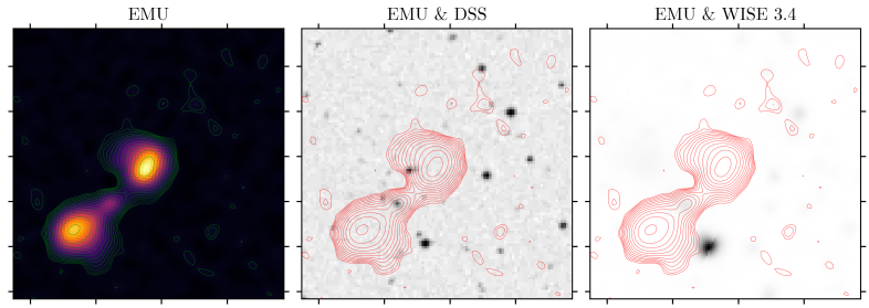
Figure 1: Example cutout as presented to the participants of the experiments detailed in Sections 2.2 and 2.3. Cutout centre: 21h 02m 16s -54^∘ $23^{\prime}$ $36^{\prime\prime}$ (J2000). blackThe lowest contour is fixed at 0.12 mJy. Subsequent contours are multiples of $\sqrt{2}$ higher.

2.2 Plain English Annotations

To derive the desired plain English taxonomy, we started with plain English descriptions (annotations) of the given object or phenomenon. Using the 299 sets of images outlined in Section 2.1, we built a private Zooniverse project, where we presented users with an empty text box and a prompt reading:

Please describe the source:

• in the middle of the frame and any associated emission.

• use simple English.

• avoid jargon.

  • e. g. refrain from typing FRI, WAT, etc.

• descriptions should be separated by “,”.

This data was intentionally collected to be relatively unconstrained to encourage the annotations to cover diverse ideas of source features. Thus users were enabled to highlight and describe whatever caught their attention within the image. The trade-off in this unstructured description approach is that the resulting data are unwieldy and noisy (the consistency and formatting of phrases is not constrained). As such, the method outlined in Section 3 contains a significant overhead of data cleaning which is common with any unstructured natural language data.

The data collection for this experiment ran from the 17^th of December 2021 to the 27^th of January 2022. We offered users who processed more than 100 sources co-authorship on this publication which is a direct result of their efforts. In total, we had 19 users annotate an average of 154 sources each, resulting in a total of 2,920 descriptions consisting of a black8,486 comma separated annotations. Almost all of these users are astronomers, and more than three quarters of them have at least some academic experience of radio morphologies.

2.3 Expert Classification

We conducted a second experiment to collect expert classifications on the same sets of images. This experiment was conducted with the aim of extracting ideas represented by annotations which are relevant to the expert’s science cases.

We established a separate private Zooniverse project and invited a number of experts to participate in classifying the radio morphologies of the objects in the images described in Section 2.1. To classify objects with predefined classes participants were prompted with:

Radio Morphology: Please describe the source:

• in the middle of the frame and any associated emission

• select one or more tags that fit object radio morphology.

We presented the participants with 22 classes, which they could use as they wished, including assigning none or all of them to the subject. The abstract classes listed were selected from a compiled list of radio morphology classes presented in Rudnick (2021) and were: Single, Double, Classical double, Triple, Narrow-angle tail (NAT), Wide-angle tail (WAT), Bent tail, Fanaroff & Riley Class 1 (FR I), Fanaroff & Riley Class 2 (FR II), Fanaroff & Riley Class 0 (FR 0), Hybrid, X-shaped, S-shaped, C-shaped, Diffuse, Double-double (DDRG), Core-dominant, Core-jet, Compact Symmetric Object (CSO), 1-sided, Odd Radio Circle (ORC), and Star-Forming Galaxy (SFG). This experiment ran from the 27^th of January to the 19^th of May 2022. 5 experts made a total of 1,257 multi-label classifications of an average 251 objects each.

3 Method

To the best of our knowledge, there is no existing process or NLP approach which produces a semantic taxonomy from a corpus of short annotations. The closest approaches are widely used topic modelling approaches. These approaches capture topics within a corpus through distributions of terms in documents. Vayansky & Kumar (2020) present a helpful review of topic modelling variants. These models are designed to return a distribution of terms which belong to each discovered topic. They are not designed to return terms which communicate what a given topic is. We explicitly want to build a taxonomy on a certain subject. Therefore the terms which effectively capture the meaning of a topic are essential.

Although a panel of experts may be able to manually define a semantic set of terms for a given problem, the success of such an approach would depend on whether the panel agree, the backgrounds of the experts, and their ability to distil complex ideas into simple plain English effectively. This manual approach would likely also lack the reproducibility and tractability that is expected by the physical sciences.

We therefore propose a method through which short annotations are distilled into semantic tags in accordance with a specific science case and its respective features (including classes). The workflow of the method is presented in Figure 2. The derived taxonomy should provide wide coverage of objects of interest, have the ability to distinguish features, be clear in what semantic feature it describes, and be appropriate to the science cases.

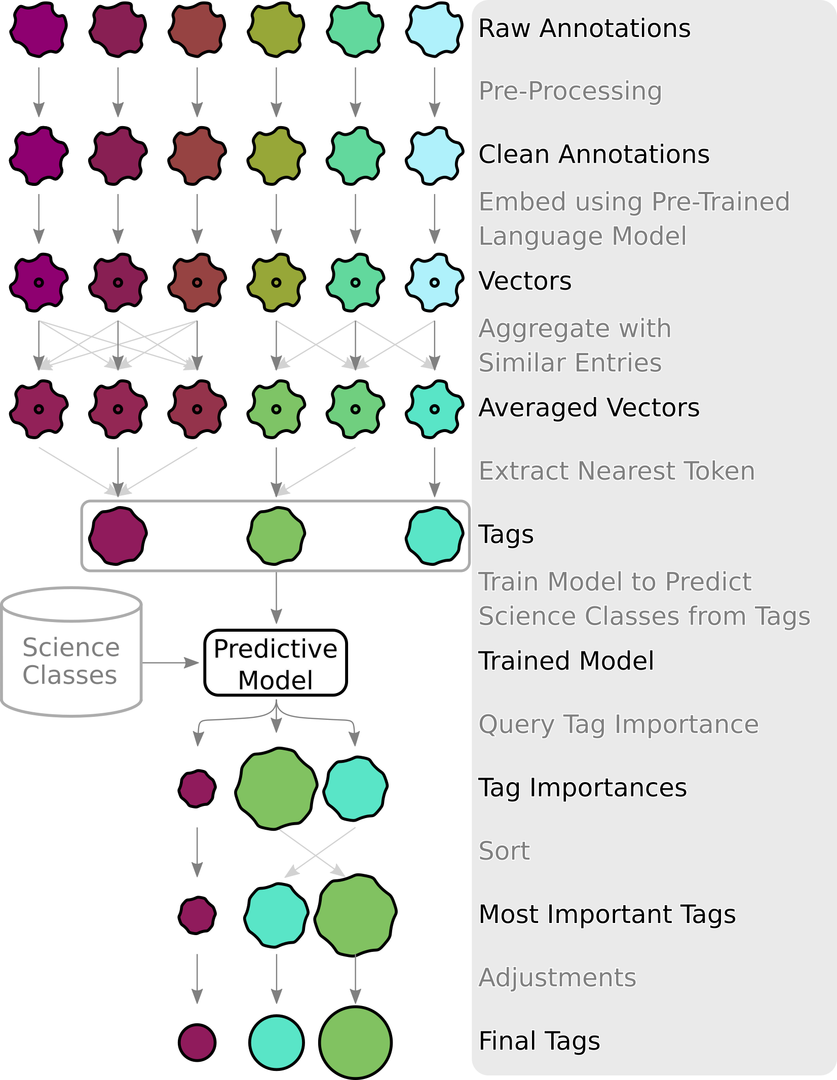
Figure 2: Proposed workflow to computationally derive a semantic plain English taxonomy from a set of annotations.

Conceptually, in the framework similar annotations are aggregated to produce a single term which we call ‘tag’. We rank how important tags are based on the impact they have in classifying the existing abstracted science classes. A selection is made on the most important tags to form a taxonomy.

A technical outline of the method is presented in Section 3.1. The implementation details for our data and project are presented in Section 3.2.

3.1 Technical Outline

Sequences of words are processed where $w_{i}$ represents the $i^{th}$ word of $N$ in a given annotation, $\mathbf{a}_{j}=\left(w_{1},w_{2},...,w_{N}\right)$. Here $\mathbf{a}_{j}$ is the $j^{th}$ annotation of the $M$ annotations in our corpus. Note that in the NLP literature, the equivalent of annotations would be ‘documents’. This method is expected to work best on extremely short annotations (documents), where each annotation contains a single idea. The annotations are embedded into a $k$-dimensional vector through a pre-trained model, $f_{\text{emb}}$:

$$f_{\text{emb}}\left(\mathbf{a}_{j}\right)=\mathbf{v}_{j}\in\mathbb{R}^{k}.$$ (1)

This is currently implemented such that the order of the words does not affect the encoding (i.e. in a bag-of-words paradigm). We embed each word within an annotation through

$$f_{\text{emb}}\left(\mathbf{a}_{j}\right)=\frac{1}{N}\sum_{i=1}^{N}f_{\text{emb}}\left(w_{i}\right).$$ (2)

For pairs of annotations, $(i,j)\in[1,M]^{2}$, a similarity value is calculated using the cosine similarity, $g_{\text{cs sim}}:\mathbb{R}^{k}\xrightarrow[]{}[-1,1]$, which takes the dot product of two vectors scaled by the inverse of the product of the euclidean norms of those vectors:

$$g_{\text{cs sim}}(\mathbf{v}_{i},\mathbf{v}_{j})=\frac{\mathbf{v}_{i}\cdot\mathbf{v}_{j}}{\lVert\mathbf{v}_{i}\rVert\lVert\mathbf{v}_{j}\rVert}.$$ (3)

According to a similarity threshold, $\sigma$, $M$ averaged vectors are then calculated through:

$${v}_{i}^{\prime}=\frac{1}{M^{\prime}}\sum_{j=1}^{M}\begin{cases}\mathbf{v}_{j}&\text{if\hskip 10.0pt}g_{\text{sim}}(\mathbf{v}_{i},\mathbf{v}_{j})\geq\sigma\\ 0&\text{else,}\end{cases}$$ (4)

where $M^{\prime}$ is the number of non-zero elements being summed over. The model, $f_{\rm emb}$, used to embed the annotations is then used to produce the token which is closest to $\mathbf{v}^{\prime}_{i}$:

$$f_{\text{emb}}^{-1}(\mathbf{v}^{\prime}_{j})\approx s_{q},$$ (5)

where $s_{q}$ is the $q^{th}$ entry of all $Q$ unique derived tags. As tags are derived from the $M$ annotations $Q\leq M$.

For each annotated object, we define $\mathbf{t}=(t_{1},...,t_{Q})$ as a vector encoding of the tags, where $t_{q}$ is 1 if that tag was present in an annotation associated with that object, or 0 if that tag is not associated with it. As each object has multiple individual annotations associated with it, it can be described through its derived tags $\mathbf{t}\in\{0,1\}^{Q}$.

We consider each science class $y$ in the set of science classes $Y$. Using the encoded tag vector, $\mathbf{t}$, for each object, we fit a model, $f_{y}:\{0,1\}^{Q}\xrightarrow[]{}\{0,1\}$, to predict the presence of each science class $y\in Y$. For each model, $f_{y}$, and tag representation, $t_{q}$, we calculate an importance

$$f_{\text{Importance}}(f_{y},t_{q})=I_{(q,y)}\in\mathbb{R},$$ (6)

where a larger value of $I_{(q,y)}$ means that $t_{q}$, and subsequently $s_{q}$, are more important to the classification output.

To recover the importance of the $q^{th}$ tag, we take an average across all models, $f_{y}$, for a given tag, $s_{q}$. We take the support weighted average of the importance of each model

$$I_{q}=\frac{1}{Q}\sum_{y\in Y}n_{y}I_{(q,y)}.$$ (7)

Here, $n_{y}$ is the number of (positive) class $y$ entries. blackNote that other weightings may be preferable depending on the available data and purpose. For instance, if a multi-objective regression task were used instead to calculate $I_{(q,y)}$, then a uniform weighting across tasks may be more appropriate. We normalise the importance values, $I_{q}$, such that

$$\sum_{q=1}^{Q}I^{\prime}_{q}=1,\text{\hskip 10.0ptand\hskip 10.0pt}I^{\prime}_{q}\in[0,1].$$ (8)

Finally, the tags, $s_{q}$, are sorted by their $I^{\prime}_{q}$. Although tags are all expected to have some non-zero $I^{\prime}_{q}$, a majority of the information is contained within the top tags. Additionally, the tags ranked lowest in this scheme are expected to be noisy (e.g. annotations which contain incorrect spellings, reference otherwise irrelevant features, or are only impactful on a given prediction through the random association of its small sample size). We set an importance threshold to select the top $Q^{\prime}<Q$ tags. These most important tags, consisting of $Q^{\prime}$ strings, $s\in S_{\text{Taxonomy}}$, is the derived taxonomy.

Some of the tags, $s$, may require clarification to allow the tag to be clear upon first reading. To do so the raw annotations which that tag was derived from are taken into consideration, in order to verify what it represents.

3.2 Implementation

The exact implementation of the method outlined in Section 3.1 will depend on the data being used. The details for our implementation are as follows.

3.2.1 Pre-Processing

The goal of pre-processing the annotations is to format the data in a uniform manner without disrupting the content (i. e. standardising grammar, spelling, and formatting). To do this, a number of common NLP data processes are applied. These are applied in the order they are presented in.

All annotations are set to lower case and all accents are removed from characters. Ampersands and new line commands are removed or replaced as appropriate. Forward slash and full stop characters are replaced with commas as they are often observed to represent separate ideas, which our method assumes are comma separated. Double whitespaces are corrected and hyphens are removed.

Based on manual inspection, additional corrections are made to a number of annotations. These are spelling mistakes such as ‘copact’ being corrected to ‘compact’. We then drop any annotations which mention ‘DSS’, ‘WISE’ or ‘optical’ as these annotations are not expected to be a comment on the radio morphology, which is our target of interest.

At this point, the sets of comma separated annotations are separated into individual annotations. Contractions are expanded. A list of stopwords is extended to include ‘like’, as well as scientific terms which the pipeline should not be affected by as they are both technical and not related to morphology. These additional stopwords include ‘emu’, ‘galaxy’, ‘galactic’, ‘emission’ and ‘source’. Terms for cardinal directions (‘north’, ‘south‘, ‘east’, ‘west’) are also added to the stopwords since our focus is on the features themselves instead of their position relative to a specific source. This stopwords list is applied to the annotations.

We consider both lemmatized and unlemmatized approaches to the data moving forward. Each annotation has now been cleaned, and the data are largely consistently formatted.

3.2.2 Embeddings

When embedding the cleaned annotations into vectors, we use SpaCy’s large English language model which is the largest available model within the SpaCy package (v3.3.0) that has tokens (largely words) embedded. It contains 685k embeddings. For a given vector, the model can return the closest embedded word(s). This feature is essential to our process, and is a key factor in the decision to use this model. Other advanced, such as transformer based models, can take word order into account, but do not have these token embeddings. In the implemented SpaCy version, the vector embeddings are learned through the GloVe algorithm introduced by Pennington et al. (2014). GloVe (Global Vectors for Word Representation) is an unsupervised representation learning algorithm which aims to embed words in a space which presents various desirable features. These features include semantic and linguistic similarity, which is advantageous for our use case.

To decide what similarity threshold to use to aggregate over, we consider the histogram of cosine similarities of all annotations. This is presented in Figure 3. This histogram is presented using annotation embeddings which were lemmatized and does not include self-similarities. The peak at 1.0 is due to tags which are identical (maximally similar). The rigorous cleaning process reducing short annotations to a few words before the annotations are embedded is likely a factor. Additionally, self-consistent vocabulary across multiple annotations may be embedded to an (essentially) identical vector.

To capture the excess tail of more similar vectors, we consider similarity thresholds above $0.5$ for our models. Lower thresholds would contain the bulk of all annotation pairs, which would be counterproductive in trying to capture individual concepts. However, we would like to explore thresholds down to $0.5$ to reduce the number of unique terms and maximise the number of entries per unique tag. The tags derived from the aggregated vector encodings, are returned by SpaCy as single tokens (words).

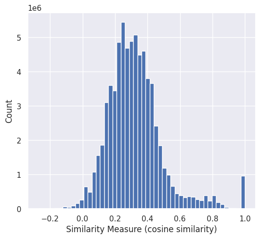
Figure 3: The histogram of the cosine similarities of the embedded annotations. Data is lemmatized and does not include self-similarity values.

3.2.3 Model Definition

We predict science classes on a source by source basis. We use 22 science classes to train the models to classify science classes from our derived tags. Three science classes presented to our expert classifiers are functionally removed as they are either not usable without spectra (Compact Symmetric Objectblack; CSO), extremely contested and largely disused (Fanaroff-Riley Class 0black; FR0, Hardcastle & Croston, 2020; Rudnick, 2021), or largely uninformative when considering blackextended radio morphology (Single). Furthermore, the following three science classes have insufficient positive cases for training: Double-Double Radio Galaxies (DDRG; Schoenmakers et al., 2000), Hybrid Morphology Radio Sources (HyMoRS; Banfield et al., 2015; Kapińska et al., 2017), and Odd Radio Circles (ORC; Norris et al., 2021a). The experts often did not agree with their usage of the terms. We explore what degree of agreement (expert threshold) beyond which we will consider a source as being positively classified with a certain science class in Section 4.1.

To train models that predict science classes from our derived tags, we have 299 sources. This is a small data set. We chose a relatively simple model in response. We train random forests in a one-vs-rest scheme, i. e. one random forest model to classify one science class. We treat a set of these models as a single model which predicts the multi-label target of an input. The random forests use the Gini impurity criterion, with the aim of improving the explainability of the selected features (Menze et al., 2009). The random forests are configured with 500 estimators, no maximum depth, and a seeded random state to allow for reproducible results. Unspecified features of the models are inherited from default values as implemented by Scikit-Learn v1.1.0.

3.2.4 Evaluation

Another challenge of the relatively small data set is the evaluation of the trained models. We use cross validation to maximise our use of the data. The model is evaluated through 10-fold cross validation, where we train 10 models on 10 different sets of nine tenths of the available data and evaluate each on the respectively withheld final tenth. With predictions for each tenth from one of the ten trained models, we recover predictions for each data point. These predictions result in approximate generalised performance metrics for the models.

We choose to track the performance of our models with macro and weighted F1 scores. An F1 score is the harmonic mean of precision and recall, and can be written as

$$F1=2*\frac{(precision\cdot recall)}{(precision+recall)}=\frac{TP}{TP+\frac{1}{2}(FP+FN)},$$ (9)

where $TP$ is the number of true positives, $FP$ is the number of false positives, and $FN$ is the number of false negatives. The macro and weighted F1 scores are extensions to enable evaluations of multi-label problems. The macro F1 score is calculated by averaging F1 scores calculated in a one-vs-rest scheme for each target class. The weighted F1 score is calculated identically to the macro F1 score, except that we take the weighted mean where each score is first scaled by the number of samples of a given class, which may be more telling in an imbalanced data classification problem.

3.2.5 Importance

To estimate the importance of each of the tags, we use Shapley values. Shapley values are a common explainability tool used in machine learning applications (Lundberg & Lee, 2017). These values convey how much a feature has contributed to the prediction of the respective model in comparison to the average predictions of the model. Exact Shapley values for each input tag and science classification are calculated using the trained random forest model and the SHAP package for trees introduced in Lundberg et al. (2020). These values are the importance values used to estimate which tags capture the semantics of radio morphology.

black

4 Taxonomy

4.1 Data Configuration

To evaluate which data configuration (i.e. data processing parameter selection) is best, we consider the F1 scores of models trained on various configurations of the data. We grid search data across configurations including four expert thresholds, eleven similarity thresholds, and with or without lemmatization. This results in 88 configurations, which we construct and evaluate.

For the expert classification we demand that at least 20 %, 40 %, 60 %, or 80 % of the votes made on a given source agree. We call these confidence thresholds. Note that we make use of percentages. Sources which have not been classified by all experts can still have their classifications reflected in the confidence thresholds used in this search. We do not consider 100% agreement amongst experts as so few classifications would survive that we could not train a model (highlighting a serious issue of the current classification scheme). The F1 scores are presented in Figure 4, for which the statistics of the random forest models are taken over all 22 configurations (2 lemmatization and 11 similarity threshold combinations) for each expert threshold.

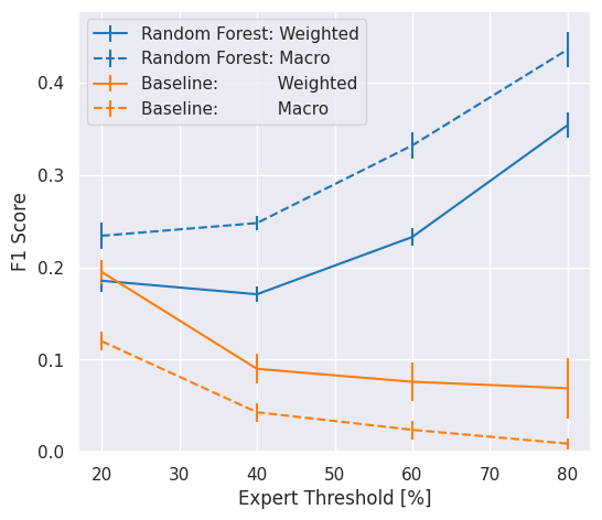
Figure 4: Aggregated F1 scores of both random forest models and baselines showing the effect of thresholding the expert classifications. The baselines are constructed by randomly predicting in accordance with the rate of positive cases per positive class. Statistics are measured over 5,000 instances of the baseline estimators, and over all lemmatization and similarity threshold configurations of the random forest models.

Simply stating that the model improves as the expert threshold is increased is largely true, see Figure 4. However, with increasing expert thresholds, the task which the model has been asked to complete becomes easier as the noise in the classifications is functionally reduced. The subset of data where experts have a high consensus are more likely to have clearly identifiable morphologies (reduced aleatoric uncertainty) or present with a morphological classification which is more widely agreed upon amongst the experts (reduced epistemic uncertainty). In an attempt to capture a broader perspective on what radio morphologies are, while maintaining accuracy of the classifications, we select an expert threshold of 60% for the remainder of this work.

Figure 5 shows the performance of the 22 models for each similarity threshold and lemmatization configuration. We select the configuration with a similarity threshold of 0.80 and lemmatized inputs. This configuration results in 213 unique tags. The model achieved a weighted F1 score of 0.254 and a macro F1 score of 0.350. This is the model with the highest weighted F1 score. The highest macro F1 score is 0.352 held by both configurations with a similarity threshold of 0.6.

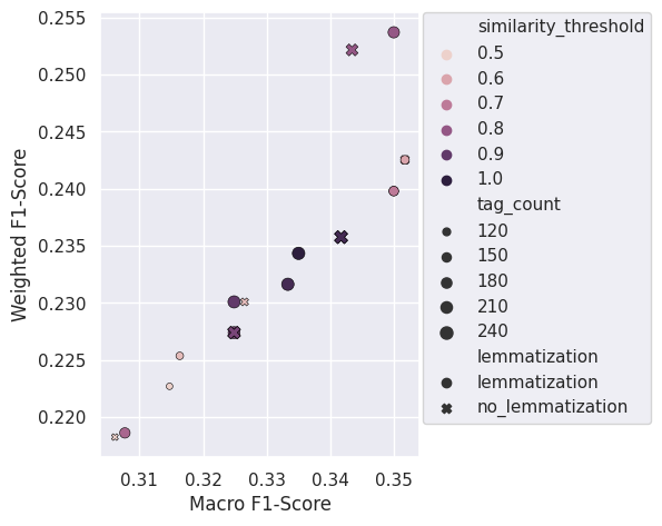
Figure 5: Grid search results across both lemmatization and the eleven similarity threshold configurations for the selected expert threshold of 60$\%$. tag_count refers to the total number of unique tags which that configuration produced, which is strongly dependant on the similarity threshold of the configuration. The selected configuration is the lemmatized version with a similarity threshold of 0.80 (expert threshold of 60$\%$).

4.2 Tag Ranking

The Shapley values are calculated for each tag provided to the model with respect to the model’s outputs and the full data set. This provides us with a Shapley value for each science class and tag combination. We take the support weighted average of the Shapley values across the science cases to provide us with a descriptive Shapley value for a given tag. We normalise these values so that they sum to one across all tags. We call these values the comparative weighted Shapley values. These are presented as percentages which reflect how much sway a given tag has over the science classification of the model.

We calculate the comparative weighted Shapley values and present the 70 most important terms in Figure 6. To select a usable volume of tags, we define the taxonomy to be the top tags required for 68% of the descriptive power to be maintained (approximately 1% of the comparative weighted Shapley value). In this data configuration, this results in a taxonomy of 33 tags.

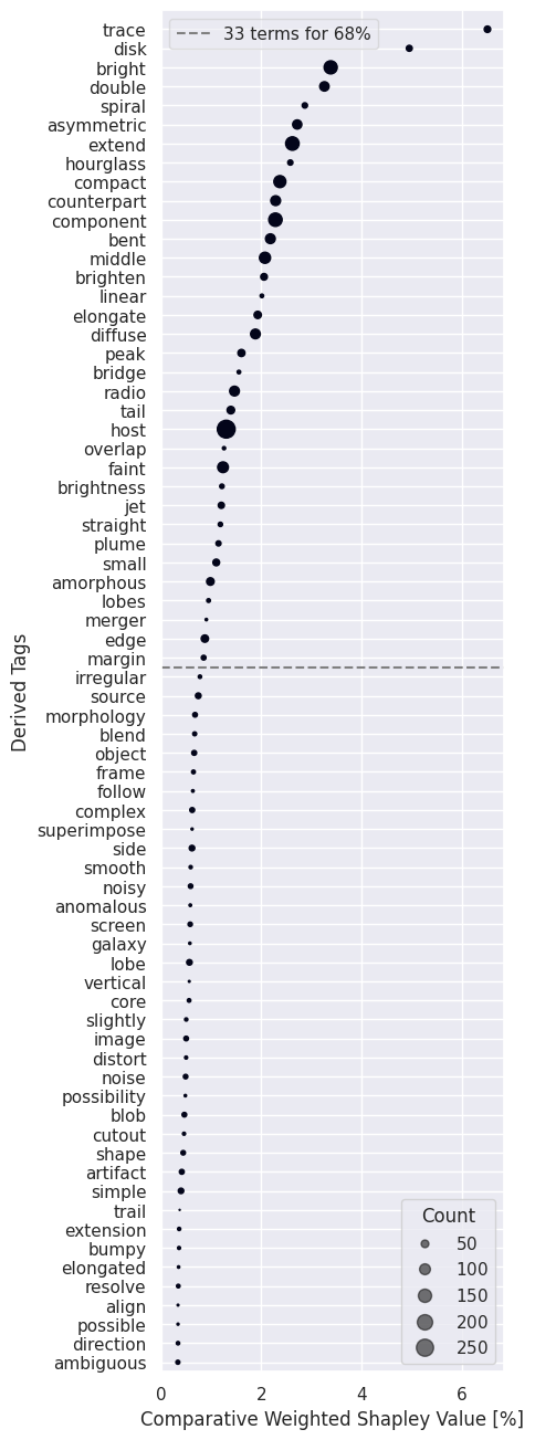
Figure 6: Top 70 tags sorted by their comparative weighted average Shapley values for the configuration selected in Section 4.1.

Highlighting the benefits of Shapley ranking over a simpler approach such as correlations, we present an interactive graph visualisation of moderately strong correlations between all combinations of both tags and science cases in Figure 7. Importantly, the graph does not contain all 33 tags. This is because most of the top 33 tags are not strongly correlated with other terms. They are still the most impactful to the model’s decision, as non-linear combinations of tags can be used to classify the science case. Their value to the non-linear classifications is captured by Shapley values.

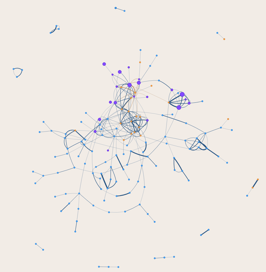
Figure 7: Still frame from the interactive graph available at https://github.com/mb010/Text2Tag/blob/main/CorrelationsGraph.html (download and open with a browser). The graph’s edges are correlations above a magnitude of 0.3. Nodes are tags from the top top 33 (purple), other tags (blue), and science classes (orange). The node sizes reflect the occurrence rate of a given node across the 299 sources. The width of the edges represents the correlation between the two nodes it connects. All correlations are in the range $[-0.5,0.9]$.

4.3 Taxonomy Adjustments

Limited to single words, the derived tags may not be an optimal selection. Suboptimal tag representations may also occur when the conjugation of a given term is relevant to the use case but lemmatization has removed it even if it would been more easily understood (e.g. ‘extended’ in comparison to ‘extend’). Furthermore, the method only outputs single words, even if the concept the tag represents is better represented by multiple terms.

We therefore investigate each tag in turn by considering all annotations which contribute to it. We adjust tags in an attempt to optimise the taxonomy for grammatical and conceptual clarity. The adjusted tags are listed below, including descriptions of the original annotations / concepts which a tag represents.

• trace: derives directly from numerous annotations stating ‘traces host galaxy’. This is a more clear expression for what this tag represents. We therefore alter ‘trace’ to ‘traces host galaxy’.

• disk: derives from annotations such as ‘emission from galaxy disk’. We therefore merge this with ‘traces host galaxy’ (originally ‘trace’). This refers to the radio emission tracing the host galaxy rather than the morphology of the host.

• bright: refers to bright features of a presented cutout. This includes cores as well as neighbouring sources. This information is more clearly contained in the catalogues of radio component fluxes. Therefore, this tag is dropped.

• spiral: derives from spiral galaxies being the hosts of the radio emission. This tag is changed to ‘traces host galaxy’ as it then contains the relevant radio morphology information.

• asymmetric: original annotations refer to asymmetric structure. To highlight the difference between asymmetric structure and brightness, we rename this tag to ‘asymmetric structure’.

• extend: Grammatical adjustment to ‘extended’.

• component: refers to the number of components which the source is composed of. This tag is dropped in favour of catalogues which list how many separated components are assigned to a source.

• counterpart: refers to matching emission in either optical or infra-red. Host identification and ‘traces host galaxy’ will capture this information. Therefore, this tag is dropped.

• middle: Largely referring to presence and features of the central core of a radio galaxy. We therefore rename this tag to ‘core’.

• brighten: Refers to ‘edge brightened’ sources. We therefore clarify this by altering this tag to ‘edge brightened’.

• linear: Refers to non bent radio morphologies, which is captured in the absence of the ‘bent’ tag. Therefore this tag is dropped.

• elongate: Refers to elongated structures in the radio emission. This is captured by the absence of the ‘bent’ tag when sources are also ‘extended’ and is therefore dropped.

• radio: Annotations were written commenting on the radio emission in general ways (such as the presence of a jet or how many components are visible). This information is all mapped by other tags / processes. For this reason, we drop this tag from the taxonomy.

• overlap: Often refers to emission which overlaps with radio contours or vice versa. It is therefore be changed to ‘traces host galaxy’.

• brightness: Original annotations almost exclusively refer to ‘asymmetric brightness’ across components or within the structure being discussed. We therefore clarify this tag by changing it to ‘asymmetric brightness’.

• straight: Refers to the non-bent structure of the radio galaxy. We therefore drop it in favour of the absence of the tag ‘bent’.

• lobes: We make a grammatical change to ‘lobe’ with the intent to make this tag less ambiguous for future users.

• edge: Highlighting clear edges of sources, as opposed to diffuse edges. This is largely equivalent to and is merged into ‘edge brightened’.

• margin: The annotations from which this tag derives refer to the source extending beyond the margins of the cutout. This is being accounted for with updated cutouts, and is not morphologically relevant beyond the angular extent of a source, which is better presented in a catalogue format.

4.4 Semantic Taxonomy

After the adjustments made to the tags in Section 4.3, we have 22 unique semantic tags. In alphabetical order, the semantic tags we propose to use for radio galaxy morphology are: amorphous, asymmetric brightness, asymmetric structure, bent, bridge, compact, core, diffuse, double, edge brightened, extended, faint, host, hourglass, jet, lobe, merger, peak, plume, small, tail, and traces host galaxy.

4.5 Effectively Assigning Tags

We have succeeded in deriving semantic tags for radio morphologies (see Section 4.4). However, for RGZ EMU and other citizen science approaches it is not effective to ask citizen scientists to use 22 tags. Terms would likely be ignored in a long list, and users would easily bottleneck on a small number of tags, neglecting the remainder of the taxonomy. This would be detrimental to both the science case and the user experience.

To improve the scientific results as well as the user experience, and to make the most effective use of the citizen scientists’ time and energy, we consider which tags within the taxonomy can be most easily computed algorithmically at other stages of processing, e.g. ‘small’ is easily calculated through the angular extent of the assembly mask for a given source. We aim for 10 tags which can be presented on a single screen to the citizen scientists. We consider each term in turn, and outline how each term might be assigned in Table 1.

Proposed for Algorithmic Assignment
asymmetric brightness	Integrated flux ratio between source sections.
asymmetric structure	Symmetric components around host.
compact	Angular extent of the components.
diffuse	Proportion of assembly mask with emission.
double	A ‘component’ number of two.
edge brightened	Relative radial brightness distribution.
extended	Angular extent of the source.
faint	Integrated relative flux.
host	Whether or not a host is identifiable.
peak	Peak within the assembly mask.
small	Angular extent of assembly mask.
traces host galaxy	Assembly mask and host emission correlation.
Proposed for Tagging
amorphous, bent, bridge, core, hourglass, jet, lobe, merger, plume, tail

Table 1: A summary of the suggestions on how the tags of the final adjusted taxonomy are to be assigned. ‘Assembly mask’ refers to a mask derived from the source assembly process where multiple source components are grouped as (likely) belonging to a single source. ‘Tagging’ refers to citizen science support, or calibrated and trained machine learning models.

The tags which we believe are least easily computed will benefit the most from citizen scientist input. These are the tags which are presented as ‘proposed for tagging’ in Table 1. These ten tags are those which the RGZ EMU project will present to its citizen scientist volunteers.

4.6 RGZ EMU Early Feedback

While working towards our final release of RGZ EMU, we asked a small group of 16 testers who have never worked on radio galaxy studies before (8 from China, 7 from Pakistan and 1 from Germany) for feedback on an early version of the tags terms provided by a beta version of the pipeline presented in this work. The tags presented to the testers were: bent, bridge, complex, diffuse, distorted, elongated, hourglass, jet, plume, tail.

In general, our testers found most provided tags self explanatory. The main concern which the testers raised, was around the definition of three words they were not very familiar with: ‘plume’, ‘tail’ and ‘elongated’. We believe there are two main contributions to this phenomena:

1. Our testers were all non-native English speakers, which is likely to explain their struggle with the meaning of ‘plume’,

2. The testers showed differences in their thinking around terms. For example, this included describing ‘elongated’ as ‘extended’, ‘tail of a comet’, ‘oval shape’, or a ‘jet-like structure’.

To address these concerns, the final workflow blackwill contain examples and conceptual definitions (see Appendix A) which users can reference for guidance. Furthermore, the RGZ EMU team is considering the translation of the tags into multiple languages, where issues such as this may be less relevant.

black

5 Radio Astronomy Challenges and Semantic Morphologies

black The semantic taxonomy derived in this work (Section 4.4) is expected to be most useful as a tool by which astronomers can select samples of radio galaxies from source catalogues in a flexible manner. Assuming each of the tags is present or not, we can estimate how many populations can be selected. For the full taxonomy of 22 tags, $2^{22}=4\,194\,304$ populations can be selected ($2^{10}=1\,024$ for the ten tags that RGZ EMU citizen scientists will use; see Section 4.5).

blackIn practice, the number of populations that the tags map may be quite different. For example, the binary estimate presented here does not consider the use of other catalogued features, such as flux, spectral index, or redshift. It also does not take into account that certain tags may be fundamentally correlated. Additionally, one might expect that given enough data, catalogues containing vote fractions for each tag could enable uncertainty and strength estimates, i.e. how ‘bent’ a source might be could be approximated by the fraction of citizen scientists which return the tag for that source.

black To demonstrate the utility of such semantically selected samples, we here synthesise a catalogue and perform some example selections. To synthesise our small data set into a catalogue, we estimate the tags for this catalogue by considering a source to have been assigned a given semantic tag if at least one of its annotations maps onto one of the tags in our final taxonomy. In this way, we treat our source annotations as a tagged catalogue. Future catalogues will likely improve upon this synthesised catalogue through multiple individuals making direct use of available semantic tags.

black We use this pseudo catalogue to demonstrate the impact that catalogues using a semantic taxonomy can have by considering two practical use cases. Firstly, we demonstrate the recovery of an existing population of radio galaxies in Section 5.1. We then highlight our ability to find morphological outliers in Section 5.2.

black

5.1 Detecting Traditional Populations

black We demonstrate how traditional populations can be recovered by recovering star-forming galaxies. We do this by considering sources tagged with traces host galaxy. In practice we query our data for sources which were originally tagged with ‘trace’. This is the closest proxy to ‘traces host galaxy’ tag that we can produce with our current data (see Sections 4.2 and 4.3).

blackBy simply considering sources with the ‘trace’ tag, we identify 38 objects. These are listed along side their respective expert star-forming galaxy (SFG) classification and estimated tags in Table 2. This simple approach recovers 33 of the 45 sources labelled as SFGs by our experts (with at least 60$\%$ expert agreement).

No.	Coordinates (J2000)	Expert SFG Classification	Tags
1	20h 22m 17s -55${}^{\circ}42^{\prime}52^{\prime\prime}$	✓	asymmetric structure, compact, double, faint, host, peak, traces host galaxy
2	20h 22m 31s -55${}^{\circ}16^{\prime}45^{\prime\prime}$	✓	amorphous, extended, host, traces host galaxy
3	20h 23m 00s -54${}^{\circ}59^{\prime}23^{\prime\prime}$	✓	amorphous, bent, compact, core, host, traces host galaxy
4	20h 23m 12s -53${}^{\circ}55^{\prime}43^{\prime\prime}$	✓	compact, diffuse, host, tail, traces host galaxy
5	20h 26m 02s -55${}^{\circ}36^{\prime}02^{\prime\prime}$	✓	bent, bridge, double, faint, host, hourglass, peak, traces host galaxy
6	20h 26m 53s -53${}^{\circ}56^{\prime}33^{\prime\prime}$	✓	amorphous, diffuse, host, traces host galaxy
7	20h 29m 31s -56${}^{\circ}44^{\prime}34^{\prime\prime}$	✓	amorphous, extended, host, traces host galaxy
8	20h 29m 44s -57${}^{\circ}57^{\prime}21^{\prime\prime}$	✓	bridge, core, double, extended, faint, host, peak, traces host galaxy
9	20h 31m 29s -53${}^{\circ}44^{\prime}17^{\prime\prime}$	✓	amorphous, extended, faint, host, peak, traces host galaxy
10	20h 31m 52s -53${}^{\circ}46^{\prime}30^{\prime\prime}$	✓	amorphous, compact, core, extended, host, merger, peak, traces host galaxy
11	20h 32m 02s -53${}^{\circ}37^{\prime}56^{\prime\prime}$	✓	amorphous, compact, extended, host, merger, peak, traces host galaxy
12	20h 34m 02s -52${}^{\circ}58^{\prime}50^{\prime\prime}$	✓	diffuse, extended, faint, host, traces host galaxy
13	20h 35m 33s -57${}^{\circ}22^{\prime}44^{\prime\prime}$	✓	amorphous, compact, extended, faint, host, traces host galaxy
14	20h 36m 11s -57${}^{\circ}09^{\prime}38^{\prime\prime}$	✓	compact, core, extended, faint, host, peak, traces host galaxy
15	20h 38m 19s -54${}^{\circ}05^{\prime}49^{\prime\prime}$	✓	host, merger, peak, small, traces host galaxy
16	20h 40m 18s -55${}^{\circ}16^{\prime}18^{\prime\prime}$	✓	compact, diffuse, extended, host, traces host galaxy
17	20h 40m 36s -53${}^{\circ}15^{\prime}53^{\prime\prime}$	✓	bent, bridge, extended, host, merger, traces host galaxy
18	20h 41m 09s -55${}^{\circ}28^{\prime}19^{\prime\prime}$	✓	compact, double, extended, host, traces host galaxy
19	20h 43m 10s -53${}^{\circ}27^{\prime}55^{\prime\prime}$	✓	compact, faint, host, peak, small, tail, traces host galaxy
20	20h 43m 41s -57${}^{\circ}02^{\prime}09^{\prime\prime}$	✓	diffuse, extended, host, traces host galaxy
21	20h 43m 55s -57${}^{\circ}20^{\prime}04^{\prime\prime}$	✓	amorphous, compact, core, extended, faint, host, merger, peak, traces host galaxy
22	20h 50m 42s -55${}^{\circ}47^{\prime}58^{\prime\prime}$	✓	diffuse, extended, faint, host, traces host galaxy
23	20h 53m 05s -56${}^{\circ}25^{\prime}08^{\prime\prime}$	✓	amorphous, compact, extended, host, traces host galaxy
24	20h 53m 43s -54${}^{\circ}02^{\prime}26^{\prime\prime}$	✓	compact, extended, faint, host, peak, traces host galaxy
25	20h 55m 25s -54${}^{\circ}45^{\prime}40^{\prime\prime}$	✓	amorphous, asymmetric structure, compact, extended, host, traces host galaxy
26	20h 55m 35s -55${}^{\circ}05^{\prime}54^{\prime\prime}$	✓	bent, core, diffuse, extended, host, lobe, peak, tail, traces host galaxy
27	20h 59m 43s -53${}^{\circ}58^{\prime}52^{\prime\prime}$	✓	amorphous, compact, extended, host, traces host galaxy
28	20h 59m 56s -55${}^{\circ}33^{\prime}47^{\prime\prime}$	✓	diffuse, double, edge brightened, extended, faint, host, hourglass, peak, traces host galaxy
29	21h 00m 39s -54${}^{\circ}29^{\prime}13^{\prime\prime}$	✓	amorphous, compact, core, host, peak, traces host galaxy
30	21h 01m 13s -57${}^{\circ}14^{\prime}26^{\prime\prime}$	✓	compact, extended, faint, host, peak, small, traces host galaxy
31	21h 01m 49s -57${}^{\circ}56^{\prime}45^{\prime\prime}$	✓	amorphous, compact, diffuse, host, traces host galaxy
32	21h 02m 10s -55${}^{\circ}04^{\prime}42^{\prime\prime}$	✓	core, diffuse, extended, host, peak, traces host galaxy
33	21h 06m 19s -56${}^{\circ}48^{\prime}27^{\prime\prime}$	✓	asymmetric brightness, compact, diffuse, extended, host, traces host galaxy
34	20h 22m 36s -56${}^{\circ}16^{\prime}25^{\prime\prime}$	$\times$	asymmetric structure, compact, double, faint, host, peak, small, tail, traces host galaxy
35	20h 24m 45s -56${}^{\circ}20^{\prime}47^{\prime\prime}$	$\times$	asymmetric structure, compact, faint, host, small, traces host galaxy
36	20h 47m 46s -56${}^{\circ}44^{\prime}04^{\prime\prime}$	$\times$	asymmetric structure, compact, core, diffuse, extended, host, tail, traces host galaxy
37	20h 58m 37s -57${}^{\circ}56^{\prime}39^{\prime\prime}$	$\times$	compact, host, traces host galaxy
38	20h 59m 51s -57${}^{\circ}51^{\prime}21^{\prime\prime}$	$\times$	bent, compact, core, double, extended, faint, host, peak, small, traces host galaxy

Table 2: blackSources selected for the traces host galaxy tag (‘trace’ in practice; see Section 5.1). Using an expert threshold of $60\%$ (see Section 4.1) we confirm whether or not the sampled sources are SFGs. For each source, the tags are listed in alphabetical order.

black Five sources with the ‘trace’ tag were not classified as SFGs in our expert classification scheme, i.e. 34 – 38 in Table 2. Images of these sources are presented in Figure 8, where their radio contours are shown overlaid on optical data from the Dark Energy Survey (DES; Abbott et al., 2018). Combining the deeper and higher resolution DES optical data into an RGB image aids visual interpretation compared to using DSS greyscale images. Now the primary choice for the EMU Zoo project, DES data were not initially used due to concerns about accessibility and coverage. Each of these sources is discussed individually below with respect to the optical morphology catalogues presented in Walmsley et al. (in prep.) made with the Zoobot package (as described in Walmsley et al., 2022), where the percentage of people who would have answered with a given feature is stated behind each catalogued feature.

blackSource 34 is a smooth ($78\%$) cigar shaped ($70\%$) galaxy (could be an edge-on galaxy). Source 35 is a featured ($82\%$) face-on ($98\%$; not edge-on) spiral ($73\%$) galaxy without a bar ($70\%$). Due to selection cuts, Source 36 was not included in the Walmsley et al. (in prep.) catalogues; however, the radio emission is expected to stem from at least two small galaxies bounded by the contours in the image. Source 37 is a smooth ($67\%$) round ($59\%$) galaxy. Source 38 is a featured ($91\%$) face-on ($98\%$; not edge-on) spiral ($98\%$) galaxy. It does not have a bar ($71\%$) but has a small bulge ($80\%$) and tightly wound spiral arms ($83\%$).

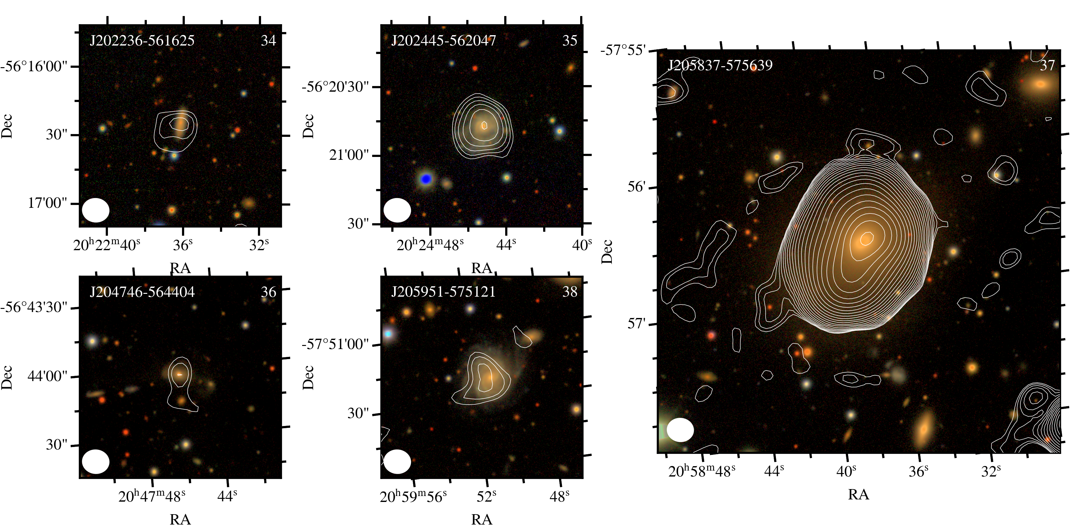
Figure 8: Sources 34-38 from Table 2 tagged with trace (selected as a proxy for ‘traces host galaxy’) which are not classified as SFGs by experts. EMU radio brightness contours matching those in Figure 1 with DES cutouts, combining g, r, and i band data into an RGB image following Lupton et al. (2004). Sources are annotated with their source numbers and (J2000) coordinates as presented in Table 2. Each source is shown to the same angular scale, as highlighted by the radio beam size in the bottom left of each panel.

blackConsequently, of the five sources initially not classified as SFGs, when reconsidered with the deeper DES (Abbott et al., 2018) images and optical morphology catalogues, it is clear that at least two sources (35 and 38) are star-forming spiral galaxies. It is likely that the experts simply did not feel confident in classifying these sources as SFG with the limited resolution and sensitivity of the DSS data.

black Twelve additional sources that were classified as SFGs with 60% agreement amongst our experts, but that did not have the ‘trace’ tag assigned to them are presented in Table 3. If the selection had been made on ‘traces host galaxy‘, rather than ‘trace’, then these sources would have been included in Table 2. This is because ‘traces host galaxy’ is derived through multiple tokens such as ‘counterpart’ (see Section 4.3).

No.	Coordinates (J2000)	Tags
1	20h 32m 03s -53${}^{\circ}44^{\prime}35^{\prime\prime}$	amorphous, compact, core, extended, host, traces host galaxy
2	20h 34m 13s -54${}^{\circ}01^{\prime}30^{\prime\prime}$	asymmetric structure, compact, core, faint, host, tail, traces host galaxy
3	20h 36m 30s -57${}^{\circ}07^{\prime}19^{\prime\prime}$	asymmetric structure, compact, extended, host, small, traces host galaxy
4	20h 44m 36s -57${}^{\circ}37^{\prime}29^{\prime\prime}$	asymmetric structure, compact, extended, faint, host, small, tail, traces host galaxy
5	20h 32m 59s -55${}^{\circ}38^{\prime}04^{\prime\prime}$	compact, host, lobe
6	20h 33m 34s -54${}^{\circ}31^{\prime}22^{\prime\prime}$	amorphous, compact, extended, host, merger, peak
7	20h 34m 49s -54${}^{\circ}12^{\prime}39^{\prime\prime}$	amorphous, compact, diffuse, double, extended, host, hourglass
8	20h 41m 41s -56${}^{\circ}10^{\prime}21^{\prime\prime}$	amorphous, compact, double, faint, host, merger, peak
9	20h 46m 26s -54${}^{\circ}00^{\prime}51^{\prime\prime}$	diffuse, double, host
10	20h 55m 12s -54${}^{\circ}31^{\prime}25^{\prime\prime}$	amorphous, compact, extended, host, merger, small
11	20h 56m 44s -56${}^{\circ}37^{\prime}48^{\prime\prime}$	compact, diffuse, double, extended, host, merger
12	21h 02m 57s -54${}^{\circ}29^{\prime}35^{\prime\prime}$	amorphous, asymmetric structure, bent, core, diffuse, faint, host, peak, tail

Table 3: blackSources which had expert SFG classifications (above 60% agreement) but were not selected through ‘trace’ as described in Section 5.1 and used for Table 2.

With a consistent use of the ‘traces host galaxy’ tag, the remaining eight SFG sources from Table 3 (sources 5 – 12) are likely to be tagged as such, as their radio emission do largely trace the respective optical host (see Appendix B).

black Of the 45 sources our experts classified as SFGs, the selection of traces host galaxy would have recovered at least 82% (33 and 4 from Tables 2 and 3 respectively) of these sources, making it a strong candidate to select SFG populations from future catalogues and highlighting how such a catalogue can be used.

black

5.2 Rare Source Detection

We here highlight the flexibility and practicality of our taxonomy by considering a combination of tags that a radio astronomer might consider to be abnormal. We query to find a source which black a) appears to be a merger, black b) presents bridged features and black c) is not faint. The result is a single entry: blacksource 17 from Table 2, shown in Figure 9.

Figure 9: blackRare source selected from the synthesised initial semantic tag catalogue by querying “hourglass $\setminus$ (amorphous $\cup$ traces host galaxy $\cup$ bent)” (set theory notation). EMU radio brightness contours matching those in Figure 1 ontop of a DES cutout prepared as in Figure 8.

blackThis source is, as expected, an unusual object requiring expert followup. It is a composite of emission from a flocculant spiral face-on 2MASS galaxy (Skrutskie et al., 2006), plus apparently associated emission to its SE with no obvious separate optical counterpart. black The burned out (blue) object at the southern edge of the contours is listed as two stars in the Gaia catalogues (Gaia Collaboration et al., 2016, 2021), and has no obvious connection to the radio structure. A very careful evaluation of the chances for serendipity, and the possible physical nature of this source, are beyond the scope of this paper. However, the control provided by these semantic tags has allowed for the selection of an unusual object worthy of further study.

6 Discussion and Impact

black

6.1 Taxonomy

blackThe proposed semantic tags will find immediate use in the RGZ EMU citizen science project (Tang $\&$ Vardoulaki et al. in prep.). For future implementations of science tags being assigned to sources, we suggest that the community uses a hash symbol to denote the use of a tag (e.g. ‘#compact’) as suggested in Rudnick (2021) to distinguish from traditional classification frameworks. This should prove useful to the legibility and analysis of future catalogues and works.

This is the first step of the tagging framework in radio astronomy morphology. The taxonomy is intentionally designed to be extensible, such that when the community decides a feature of interest is not being captured by the current version of the taxonomy blackit can be updated to include the appropriate tag. The presented set of semantic tags are a first step towards mapping common features of radio morphologies using plain English annotations.

The specificity of the tags in comparison to the current classification scheme may be a concern to some astronomers. The inconsistency with which current radio morphological classifications are defined means that the language currently in use does not have the desired specificity either - regardless of how specific a term is in an individual astronomer’s mind. Furthermore, we highlight that terms are expected to be used more consistently and clearly when selected directly rather than being derived through annotations.

A science class mapping using the semantic taxonomy is one of the goals of the RGZ EMU team. This mapping will be constructed blacktowards the end of the RGZ EMU project. This mapping should be able to provide the traditional classification of objects by predicting them based on the tags that citizen scientists have assigned to objects. It will include the most common radio morphology science classes which the community is more accustomed to. While it is hoped that the tags will span the full space of possible scientific classifications, there may be cases where the provided mapping does not cover a science case perfectly blackin its current form.

black Regardless, the ability to combine the tags to select semantic populations, as demonstrated in Section 5, will enable feature specific population studies and sources to be omitted if they present features that are not relevant to a given science case. black

6.2 Experiment and Implementation

blackAs described, the experimental set up of this work has a number of limitations, including the small size of the data set: given the degree of variation present across radio galaxy morphologies it is not possible to capture all abstract science classes of radio galaxies completely. For example, as stated in Section 3.2.3, ORCs are so rare that we could not train on them, and thus they are not taken into consideration in the weighted Shapley values. Such biases are therefore currently passed onto the derived and proposed semantic taxonomy.

blackAdditionally, abstract science classes based primarily on morphology do not directly encode other physically relevant information. Given sufficient information, it may be more informative to derive semantic tags directly from physical parameters, e.g. active galactic nuclei accretion rates. blackThis would encourage the derived semantic tags to carry information regarding the physics itself, rather than a proxy, e.g. abstract science classes. In practice, collecting a large enough sample with which to do this is not feasible at this time, but should be considered in future approaches blackand other domains.

blackWe use a pre-trained NLP model in our approach to this task. This model is a limitation even though it is also a key factor in the success of our implementation and experiments. For instance, the model we used only returns individual ‘tokens’, and not fully grammatically correct terms or phrases. We amend this through manual inspection and adjustments, however we recognise this is not a scalable solution, and will not be possible in all situations. We hope that future approaches will find solutions to this problem. The NLP literature is currently developing at a significant pace. We therefore urge future iterations and applications of this approach to actively re-consider which pre-trained model is used. We expect that by using the most up to date pre-trained model, future implementations will have more robust and versatile encodings of annotations and tags.

Finally, we note that the semantic radio morphology taxonomy derived in this work is inherently bound to the instrument with which the radio galaxies were imaged (ASKAP). Data from a more sensitive (e.g. SKA; Dewdney et al., 2009) or higher resolution (e.g. LOFAR long baseline Morabito et al., 2022) instrument might require additional or different semantic tags. This would be simple to implement under the proposed tagging paradigm, as it would blackbe sufficient to supplement the existing taxonomy with the appropriate semantic tags.

black

6.3 Semantic Taxonomies

blackThe proposed method, and respective task of deriving semantically meaningful tags (first outlined in Bowles et al., 2022), have the potential to impact other fields. We therefore discuss their potential impact and limitations in a domain agnostic tone.The move away from technical classes to blacksemantic language capturing features may have a broad impact across blacka number of technical fields, especially where complex classes have been defined and the field has blacksince moved beyond those initially valuable classification schemes, as is the case in radio astronomy. This could include any feature rich data product, especially where features are often repeated across classes.

The collaborative nature of science may be improved by the use of simplified blackand semantic language. Complex ideas are often shrouded in equally complex terminology, which can be highly effective when experts communicate with one another, but quickly becomes a hindrance to communicating in any other situation. Capturing features of an object using dictionary level definitions will lower the barrier to entry for established researchers blackwho are not domain experts to study blackthe features captured by the semantic language. This can blackbe a significant benefit, where domain specific terminology blackcould be blackan active barrier to communication blackin inter-disciplinary research. Additionally, blackthe use of plain English should enable scientific collaborations blackwithin a given field, i.e. between radio astronomy domain experts and astronomers who are not experts in radio morphology.

Outreach efforts blackare also blacklikely to benefit from the change to language. We hope that the simple language will reduce the barrier to entry for those who would like to become blackexperts in the respective field. This will have direct impact on the accessibility of technical fields as a whole including communities who have not had much practice in the use of scientific language. This is in perfect alignment with the educational aspects of citizen science, which are often used to engage underprivileged communities in science with the aim to inspire and empower. The hope of citizen science outreach is that students who have seen, interacted with, and blacksubsequently added to the international body of science feel empowered to pursue STEM subjects. Clearer language will improve engagement to support this goal.

The science in citizen science projects is also expected to benefit from the new language. Easily understood concepts presented by the simplified language should lead to improved usage of tags for a given source (Wald et al., 2016). blackAdditionally, the reduction in training time / effort of the citizen scientists is hoped to lower the labelling cost for projects as a whole by reducing the labelling cost for individual citizen scientists.

Deep learning and machine learning models currently learn to predict scientific classes from images black(or similarly high dimensional data). Learning to encode these classes can be quite challenging as the concepts and definitions represented by these classes can be both abstract and contentious. This may be partially addressed by training models to encode a semantic taxonomy instead, as models would learn the features instead of abstracted classes. Derived blacksemantic taxonomies presents more clearly defined concepts and may encourage models to learn a more robust feature space. This could improve the effectiveness of the encoded features of a model for various other tasks. Even in a simple use case, the more robust feature space may allow models to be more generalisable and less brittle, i.e. transferable or fine-tunable to differing data sets and tasks, which would be of immediate benefit to a number of applications.

The anglocentric nature of this work was alluded to previously. Although the language improvements, may benefit many populations, it does still marginalise those who do not speak English natively. The RGZ EMU team is considering a number of strategies to mitigate the effect of anglocentric labelling, including translation into multiple languages. However, we recognise that there are broader complex issues around use of language in science and recommend this as a topic of discussion in future work.

Finally, the ethics of deriving terms from an unstructured data set include careful consideration of the potential presence and impact of malicious agents. Caution is therefore advised when applying this process to other fields. blackIn this work, the data set used was small enough that each annotation was inspected individually.

7 Conclusions

In this work, we derive a flexible English taxonomy for radio astronomy and the respective morphological tagging. The proposed taxonomy blackof 22 semantic tags is

• the product of experiments collecting expert classifications and plain English annotations on radio source morphologies using selected cutouts from the EMU pilot survey,

• reduced to a set of 10 terms to maximise its effectiveness within citizen science projects, starting with RGZ EMU,

• derived analytically through a novel method with minimal clarifying intervention.

blackWe demonstrate the first effective use cases of the newly derived semantic morphology taxonomy. We show that using the tags we can recover

• known scientific morphologies, and

• rare sources with abnormal morphologies.

The method which was developed, detailed, and applied in this work is domain agnostic. The method

• provides a framework through which plain English annotations of complex ideas can return a ranked taxonomy on a given subject,

• can be applied to any scenarios where language is a barrier to future research,

• can increase the accessibility of complex scientific concepts by distilling concepts into simpler English for the public, collaborators, and citizen scientists.

The potential scientific impacts, applications, and communication benefits of this method and taxonomy are discussed at length in Section 6.

Data Availability

All the data used in this work is publicly available. The cutouts presented to users for annotation, anonymised annotations, and anonymised expert classifications are available at https://zenodo.org/record/7254123#.Y3d5EdLP2xE. The code written for these projects are available under https://github.com/mb010/Text2Tag.

Appendix A Tag Definitions

The below are the tags which will be used in RGZ EMU, as discussed in Section 4.5. Here we present the same definitions of the tags as we are planning on providing to the citizen scientists:

• Amorphous: having no clearly defined shape or form.

• Bent: Curved or having an angle.

• Bridge: A structure that connects from one side to another (not a jet; see below).

• Core: a central part distinct from the enveloping part.

• Hourglass: Shaped like an hourglass.

• Jet: A narrow stream of material appearing to emanate from a celestial object.

• Lobe: A roundish projecting part of something divided by a fissure / gap.

• Merger: Multiple separate things which appear to be connected or connecting.

• Plume: a long cloud of smoke or vapour resembling a feather as it spreads from its point of origin.

• Tail: Resembling an animal’s tail in its shape or position, typically extending downwards or outwards at the end of a thing.

The tags which are proposed for algorithmic assignment according to Table 1 are not defined here. They will likely be defined when respective algorithms are developed.

Appendix B Star Forming Galaxies without ‘Traces Host Galaxy’ Tag

Figure 10 presents the sources which were classified (above 60% agreement) as star forming galaxies, but were not tagged with ‘trace’ in our synthetic catalogue, as described in Section 5.1. Table 4 presents the optical morphologies of the sources listed in Table 3 produced by Walmsley et al. (in prep.), and made with Zoobot (initially described in Walmsley et al., 2022). Here source numbers align with those presented in Table 3.

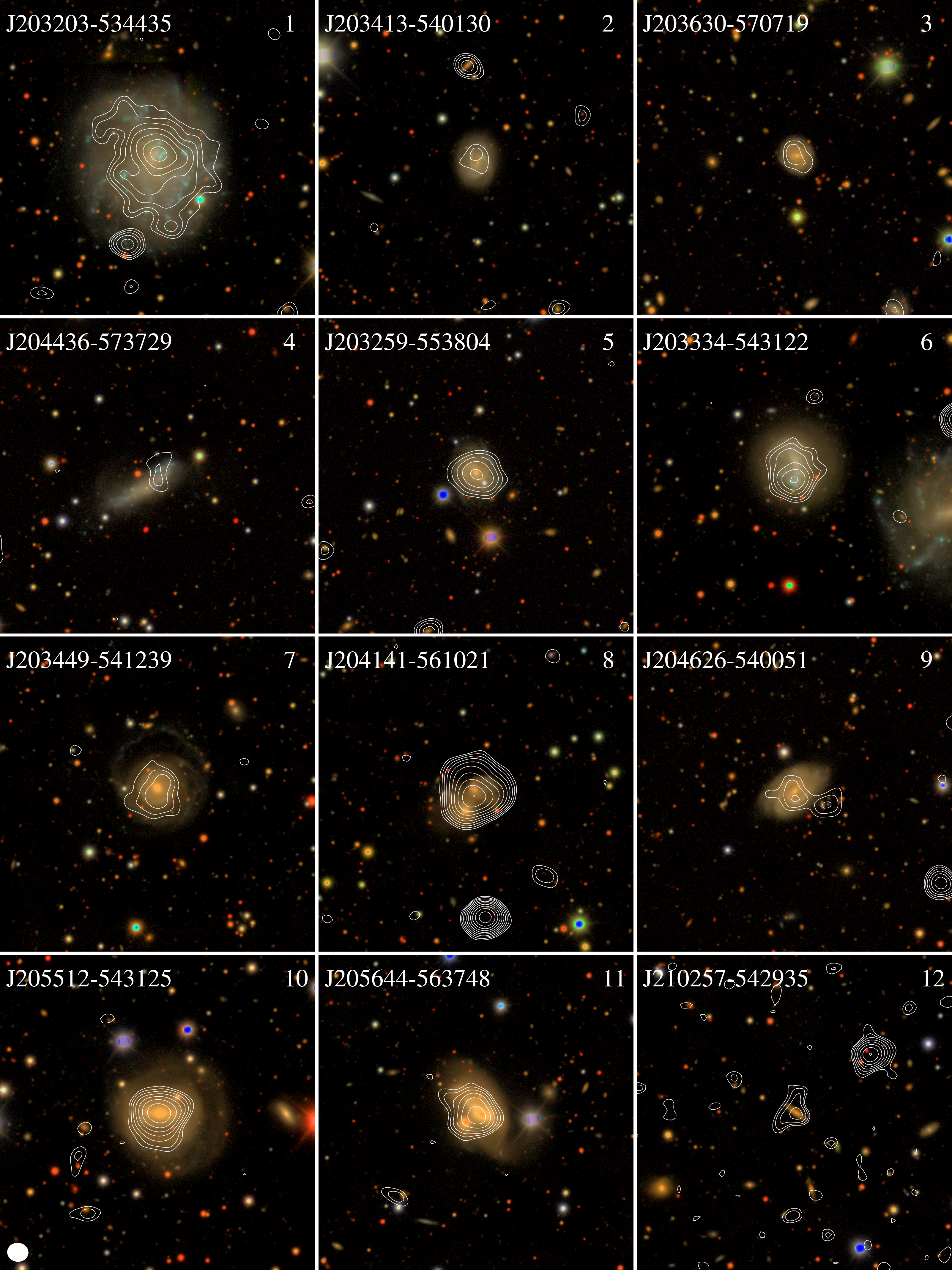
Figure 10: Composite images of SFG sources not captured by the ‘trace’ tag, as discussed in Section 5.1. EMU contours following Figure 1 with optical DES RGB backgrounds as in Figure 8. Cutout centre coordinates are presented on the image along side their respective source numbers associated with Table 3 and Table 4. The radio beam size for all panels is shown in the lower left of the figure; all cutouts are $3^{\prime}\times 3^{\prime}$.

No.	Coordinates (J2000)	GZ Morphology Predictions
1	20h 32m 03s -53${}^{\circ}44^{\prime}35^{\prime\prime}$	featured (74%; not edge-on), face-on (98%), spiral (76%), no bar (59%), small bulge (59%)
2	20h 34m 13s -54${}^{\circ}01^{\prime}30^{\prime\prime}$	featured (72%), face-on (99%; not edge-on), spiral (70%), no bar (60%), no bulge (69%)
3	20h 36m 30s -57${}^{\circ}07^{\prime}19^{\prime\prime}$	featured (89%), face-on (97%; not edge-on), spiral (98%), small bulge (85%), tight arms (76%)
4	20h 44m 36s -57${}^{\circ}37^{\prime}29^{\prime\prime}$	Not in catalogue.
5	20h 32m 59s -55${}^{\circ}38^{\prime}04^{\prime\prime}$	featured (87%), face-on (98%; not edge-on), spiral (98%), no bar (77%), small bulge (83%), tight arms (84%)
6	20h 33m 34s -54${}^{\circ}31^{\prime}22^{\prime\prime}$	featured (70%), face-on (95%; not edge-on), no spiral (68%)
7	20h 34m 49s -54${}^{\circ}12^{\prime}39^{\prime\prime}$	featured (82%), face-on (97%; not edge-on), spiral (85%), no bar (76%), moderate bulge (58%), tight arms (63%)
8	20h 41m 41s -56${}^{\circ}10^{\prime}21^{\prime\prime}$	featured (53%), face-on (96%; not edge-on), no spiral (77%), no bar (84%), merger (67%)
9	20h 46m 26s -54${}^{\circ}00^{\prime}51^{\prime\prime}$	featured (83%), face-on (98%; not edge-on), spiral (85%), small bulge (57%)
10	20h 55m 12s -54${}^{\circ}31^{\prime}25^{\prime\prime}$	Not in catalogue.
11	20h 56m 44s -56${}^{\circ}37^{\prime}48^{\prime\prime}$	featured (83%), face-on (96%; not edge-on), spiral (92%), no bar (52%), moderate bulge (59%), tight arms (68%)
12	21h 02m 57s -54${}^{\circ}29^{\prime}35^{\prime\prime}$	smooth (67%), cigar shaped (88%)

Table 4: Optical morphologies from Walmsley et al. (in prep.) of the SFG sources not captured by the ‘trace’ tag, as discussed in Section 5.1 and presented in Table 3.

Appendix C Tag Rankings

To demonstrate the contributions of our tags to the classification of a given science class, we present Figure 11, which shows the sorted most important tags for the Star-Forming Galaxy (SFG) class. Equivalent plots for each class are available in our public repository: https://github.com/mb010/Text2Tag/data/AppendixB.

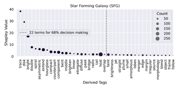
Figure 11: Class wise top Shapley value ranked tags for the Star-Forming Galaxy (SFG) science class.

References

- Abbott et al. (2018) Abbott T. M. C., et al., 2018, ApJS, 239, 18
- Adajian (2022) Adajian T., 2022, in Zalta E. N., ed., , The Stanford Encyclopedia of Philosophy, Spring 2022 edn, Metaphysics Research Lab, Stanford University
- Banfield et al. (2015) Banfield J. K., et al., 2015, MNRAS, 453, 2326
- Boch & Fernique (2014) Boch T., Fernique P., 2014, in Manset N., Forshay P., eds, Astronomical Society of the Pacific Conference Series Vol. 485, Astronomical Data Analysis Software and Systems XXIII. p. 277
- Bonaldi et al. (2019) Bonaldi A., Bonato M., Galluzzi V., Harrison I., Massardi M., Kay S., De Zotti G., Brown M. L., 2019, MNRAS, 482, 2
- Bonnarel et al. (2000) Bonnarel F., et al., 2000, A&AS, 143, 33
- Bowles et al. (2022) Bowles M., et al., 2022, NeurIPS 2022: Machine Learning and the Physical Sciences Workshop, p. arXiv:2210.14760
- Crameri (2021) Crameri F., 2021, Scientific colour maps, doi:10.5281/zenodo.5501399, https://doi.org/10.5281/zenodo.5501399
- Dewdney et al. (2009) Dewdney P. E., Hall P. J., Schilizzi R. T., Lazio T. J. L. W., 2009, IEEE Proceedings, 97, 1482
- Fanaroff & Riley (1974) Fanaroff B. L., Riley J. M., 1974, MNRAS, 167, 31P
- Gaia Collaboration et al. (2016) Gaia Collaboration et al., 2016, A&A, 595, A1
- Gaia Collaboration et al. (2021) Gaia Collaboration et al., 2021, A&A, 649, A1
- Grezes et al. (2021) Grezes F., et al., 2021. ADASS XXXI (31st annual conference on Astronomical Data Analysis Software and Systems), doi:10.48550/ARXIV.2112.00590. , https://arxiv.org/abs/2112.00590
- Hagberg et al. (2008) Hagberg A. A., Schult D. A., Swart P. J., 2008, in Varoquaux G., Vaught T., Millman J., eds, Proceedings of the 7th Python in Science Conference. Pasadena, CA USA, pp 11 – 15
- Hallinan et al. (2021) Hallinan G., Ravi V., Deep Synoptic Array Team 2021, in American Astronomical Society Meeting Abstracts. p. 316.05
- Hardcastle & Croston (2020) Hardcastle M. J., Croston J. H., 2020, New Astronomy Reviews, 88, 101539
- Hewish et al. (1968) Hewish A., Bell S. J., Pilkington J. D. H., Scott P. F., Collins R. A., 1968, Nature, 217, 709
- Honnibal & Montani (2017) Honnibal M., Montani I., 2017, spaCy 2: Natural language understanding with Bloom embeddings, convolutional neural networks and incremental parsing, To appear
- Hunter (2007) Hunter J. D., 2007, Computing in Science & Engineering, 9, 90
- Johnston et al. (2008) Johnston S., et al., 2008, Experimental Astronomy, 22, 151
- Jonas & MeerKAT Team (2016) Jonas J., MeerKAT Team 2016, in MeerKAT Science: On the Pathway to the SKA. p. 1
- Kapińska et al. (2017) Kapińska A. D., et al., 2017, AJ, 154, 253
- Lasker et al. (1990) Lasker B. M., Sturch C. R., McLean B. J., Russell J. L., Jenkner H., Shara M. M., 1990, The Astronomical Journal, 99, 2019
- Lundberg & Lee (2017) Lundberg S. M., Lee S.-I., 2017, in Guyon I., Luxburg U. V., Bengio S., Wallach H., Fergus R., Vishwanathan S., Garnett R., eds, , Advances in Neural Information Processing Systems 30. Curran Associates, Inc., pp 4765–4774, http://papers.nips.cc/paper/7062-a-unified-approach-to-interpreting-model-predictions.pdf
- Lundberg et al. (2020) Lundberg S. M., et al., 2020, Nature Machine Intelligence, 2, 2522
- Lupton et al. (2004) Lupton R., Blanton M. R., Fekete G., Hogg D. W., O’Mullane W., Szalay A., Wherry N., 2004, Publications of the Astronomical Society of the Pacific, 116, 133
- Menze et al. (2009) Menze B. H., Kelm B. M., Masuch R., Himmelreich U., Bachert P., Petrich W., Hamprecht F. A., 2009, BMC Bioinformatics, 10, 1
- Mishra & Kumar (2020) Mishra B. K., Kumar R., 2020, Natural Language Processing in Artificial Intelligence. CRC Press
- Morabito et al. (2022) Morabito L. K., et al., 2022, A&A, 658, A1
- Murphy & ngVLA Science Advisory Council (2020) Murphy E., ngVLA Science Advisory Council 2020, in American Astronomical Society Meeting Abstracts #235. p. 364.01
- Natal et al. (2021) Natal J., Ávila I., Tsukahara V. B., Pinheiro M., Maciel C. D., 2021, Entropy, 23
- Norris et al. (2011) Norris R. P., et al., 2011, Publ. Astron. Soc. Australia, 28, 215
- Norris et al. (2021a) Norris R. P., et al., 2021a, Publ. Astron. Soc. Australia, 38, e003
- Norris et al. (2021b) Norris R. P., et al., 2021b, Publ. Astron. Soc. Australia, 38, e046
- Pedregosa et al. (2011) Pedregosa F., et al., 2011, Journal of Machine Learning Research, 12, 2825
- Pennington et al. (2014) Pennington J., Socher R., Manning C. D., 2014, in Empirical Methods in Natural Language Processing (EMNLP). pp 1532–1543, http://www.aclweb.org/anthology/D14-1162
- Romm (1991) Romm J., 1991, The Sixteenth Century Journal, 22, 173
- Rudnick (2021) Rudnick L., 2021, Galaxies, 9, 85
- Schelling (1994) Schelling F. W. J. V., 1994, On the History of Modern Philosophy. Cambridge University Press
- Schoenmakers et al. (2000) Schoenmakers A. P., de Bruyn A. G., Röttgering H. J. A., van der Laan H., Kaiser C. R., 2000, MNRAS, 315, 371
- Skrutskie et al. (2006) Skrutskie M. F., et al., 2006, AJ, 131, 1163
- Southworth (1956) Southworth G. C., 1956, The Scientific Monthly, 82, 55
- Thomas et al. (2022) Thomas B., Thronson H., Buonomo A., Barbier L., 2022, Research Notes of the AAS, 6, 11
- Tingay et al. (2013) Tingay S. J., et al., 2013, Publ. Astron. Soc. Australia, 30, e007
- Vayansky & Kumar (2020) Vayansky I., Kumar S. A. P., 2020, Information Systems, 94, 101582
- Wald et al. (2016) Wald D. M., Longo J., Dobell A. R., 2016, Conservation Biology, 30, 562
- Walmsley et al. (2022) Walmsley M., et al., 2022, MNRAS, 509, 3966
- Waskom (2021) Waskom M. L., 2021, Journal of Open Source Software, 6, 3021
- Wes McKinney (2010) Wes McKinney 2010, in Stéfan van der Walt Jarrod Millman eds, Proceedings of the 9th Python in Science Conference. pp 56 – 61, doi:10.25080/Majora-92bf1922-00a
- Wolff & Holmes (2010) Wolff P., Holmes K. J., 2010, Ltd. WIREs Cogn Sci, 2, 253
- Wright et al. (2010) Wright E. L., et al., 2010, AJ, 140, 1868
- pandas development team (2020) pandas development team T., 2020, pandas-dev/pandas: Pandas, doi:10.5281/zenodo.3509134, https://doi.org/10.5281/zenodo.3509134
- van Haarlem et al. (2013) van Haarlem M. P., et al., 2013, A&A, 556, A2