11email: saniya.khan@epfl.ch 22institutetext: Dipartimento di Fisica e Astronomia, Università degli Studi di Bologna, Via Gobetti 93/2, I-40129 Bologna, Italy 33institutetext: INAF - Osservatorio di Astrofisica e Scienza dello Spazio di Bologna, Via Gobetti 93/3, I-40129 Bologna, Italy 44institutetext: School of Physics and Astronomy, University of Birmingham, Edgbaston, Birmingham, B15 2TT, UK 55institutetext: LESIA, Observatoire de Paris, PSL Research University, CNRS, Sorbonne Université, Université Paris Cité, 92195 Meudon, France 66institutetext: INAF - Osservatorio Astronomico di Padova, Vicolo dell’Osservatorio 5, I-35122 Padova, Italy 77institutetext: Leiden Observatory, Leiden University, Niels Bohrweg 2, 2333 CA Leiden, The Netherlands 88institutetext: Max-Planck-Institut für Astronomie, Königstuhl 17, 69117 Heidelberg, Germany 99institutetext: Research School of Astronomy and Astrophysics, The Australian National University, Canberra, ACT 2611, Australia 1010institutetext: ARC Centre of Excellence for All Sky Astrophysics in 3 Dimensions (ASTRO 3D), Australia
Investigating Gaia EDR3 parallax systematics using asteroseismology of Cool Giant Stars observed by
Kepler, K2, and TESS
Gaia EDR3 has provided unprecedented data that generate a lot of interest in the astrophysical community, despite the fact that systematics affect the reported parallaxes at the level of . Independent distance measurements are available from asteroseismology of red-giant stars with measurable parallaxes, whose magnitude and colour ranges more closely reflect those of other stars of interest. In this paper, we determine distances to nearly 12,500 red-giant branch and red clump stars observed by Kepler, K2, and TESS. This is done via a grid-based modelling method, where global asteroseismic observables, constraints on the photospheric chemical composition, and on the unreddened photometry are used as observational inputs. This large catalogue of asteroseismic distances allows us to provide a first comparison with Gaia EDR3 parallaxes. Offset values estimated with asteroseismology show no clear trend with ecliptic latitude or magnitude, and the trend whereby they increase (in absolute terms) as we move towards redder colours is dominated by the brightest stars. The correction model proposed by Lindegren et al. (2021a) is not suitable for all the fields considered in this study. We find a good agreement between asteroseismic results and model predictions of the red clump magnitude. We discuss possible trends with the Gaia scan law statistics, and show that two magnitude regimes exist where either asteroseismology or Gaia provides the best precision in parallax.
Key Words.:
asteroseismology — astrometry — distance scale — parallaxes — stars: distances — stars: low-mass — stars: oscillations1 Introduction
In December 2020, the early third intermediate data release of Gaia (Gaia EDR3; Gaia Collaboration et al. 2021) was published, with updated source list, astrometry, and broad-band photometry in the , , and bands. This release represents a significant improvement in both the precision and accuracy of the astrometry and photometry, with respect to Gaia DR2. While quasars yielded a median parallax of in DR2, this is now reduced to about in Gaia EDR3, with variations at a level of depending on position, magnitude and colour (Lindegren et al., 2021b).
With the EDR3 release, Lindegren et al. (2021a) (hereafter L21) proposed two offset functions and applicable to 5- and 6-parameter astrometric solutions, respectively, that give an estimate of the systematics in the parallax measurement as a function of the -band magnitude, effective wavenumber or pseudo-colour , and ecliptic latitude . Their zero-point correction model is based on quasars, and complemented with indirect methods involving physical binaries and stars in the Large Magellanic Cloud111Python implementations of both functions are available in the Gaia web pages: https://www.cosmos.esa.int/web/gaia/edr3-code..
Despite the availability of such a correction, L21 still encourage users of Gaia EDR3 data to derive their own zero-point estimates, whenever possible. Indeed, some studies dedicated to the comparison between EDR3 parallaxes and independent measurements have found that the inclusion of the L21 offset could lead to an over-correction of the parallaxes. All the values reported below give the difference between the corrected EDR3 parallaxes and the other measurements, hence positive values correspond to an over-correction, as a result of applying the L21 values222In this work, we define the residual parallax offset as , while some of the studies mentioned define it with the opposite sign, i.e. . This includes samples based on classical Cepheids (, Riess et al. 2021; and based on NIR HST and optical Gaia bands respectively, Cruz Reyes & Anderson 2023; , Molinaro et al. 2023), and RR Lyrae stars (; Bhardwaj et al., 2021). Still, there are other studies which did not report such an overestimation of the parallax zero-point, as can be seen from eclipsing binaries (; Stassun & Torres, 2021), red clump stars (, the uncertainty is not reported; Huang et al., 2021), and WUMa-type eclipsing binary systems (; Ren et al., 2021).
Following on from our Gaia DR2 study (Khan et al., 2019, hereafter K19), we extend our catalogue of distances using asteroseismic data in the Kepler, K2, and TESS southern continuous viewing zone (TESS-SCVZ) fields, allowing for a first comparison with Gaia EDR3. The asteroseismic and spectroscopic surveys used are briefly described in Sec. 2. The method for estimating asteroseismology-based parallaxes is introduced in Sec. 3. Section 4 presents our parallax zero-point results for Kepler, K2, and TESS separately, and provides a first discussion of global trends seen in ecliptic latitude, magnitude, and effective wavenumber. In Sec. 5, we discuss the magnitude of the red clump as an independent validation of the method, the impact of Gaia scanning law statistics for K2, and the existence of two regimes in magnitude where either the precision of asteroseismology or Gaia dominates. Conclusions are reported in Sec. 6.
| Fields | Baseline | () | |
|---|---|---|---|
| Kepler | 4 years | [9, 13] | [1.4, 1.5] |
| K2 | 80 days | [9, 15] | [1.35, 1.5] |
| TESS-SCVZ | 1 year | [9, 11] | [1.4, 1.5] |
2 Observational framework
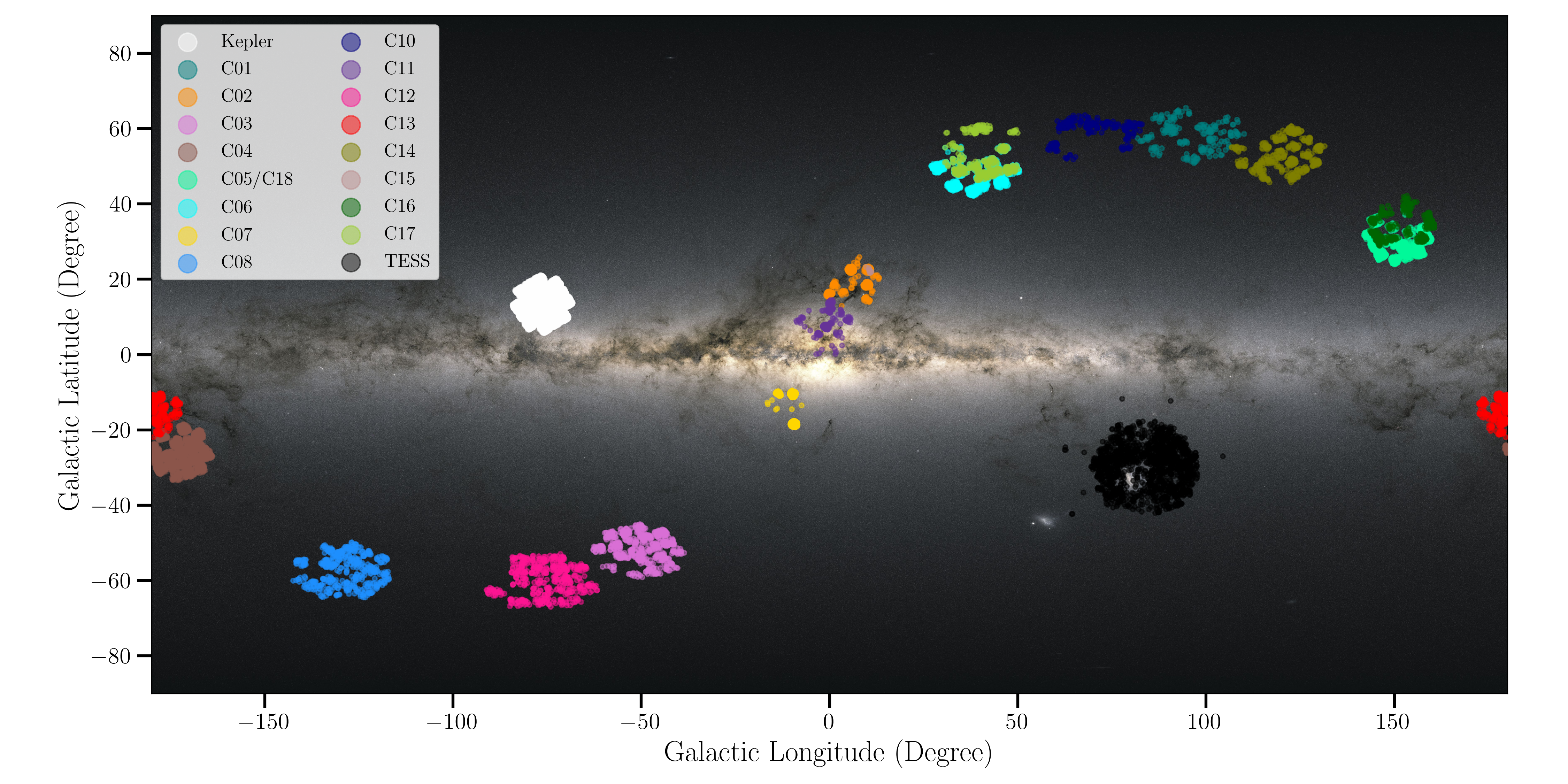
Our sample is divided into three main parts, summarised in Table 1, and the location of the various fields is illustrated on Fig. 1. The full datasets with asteroseismic, spectroscopic, and astrometric information are provided along with the paper, and details about the columns are given in App. A.
2.1 Asteroseismic information
We first have first-ascent red-giant branch (RGB) stars and red clump (RC) stars observed by Kepler (Borucki et al., 2010), for which the observation length is the longest: 4 years. The second part of our sample consists of red giants observed by K2, namely Kepler’s follow-up mission (Howell et al., 2014). Compared to the two campaigns analysed in K19, we now have data available for 17 campaigns: C01-08, C10-18. The observations of K2 campaigns have a much shorter duration of 80 days. We further analysed very bright () red-giant stars in the TESS southern continuous viewing zone (Ricker et al., 2015). The TESS full-frame images, from which the asteroseismic data are extracted, are based on 1 year of observations.
For all three surveys, we use the frequency of maximum oscillation power and the average large frequency spacing , and consider two different asteroseismic pipelines: Mosser & Appourchaux (2009, hereafter MA09) and Elsworth et al. (2020, hereafter E20). We keep stars for which both pipelines return a value in the range [15, 200] . Beyond these limits, the estimates are more uncertain and can deviate significantly between MA09 and E20.
2.2 Spectroscopic information
For K2, two different surveys are considered for constraints on the photospheric chemical composition, i.e. and (as well as , if available): APOGEE DR17 with near-infrared (NIR) all-sky spectroscopic observations and a resolution of (Abdurro’uf et al., 2022), and GALAH DR3 with southern hemisphere spectroscopic observations in the optical/NIR and (Buder et al., 2021). For Kepler and TESS, we only use APOGEE constraints. Additional flags are also applied following recommendations specific to each spectroscopic survey333We used the STAR_WARN and STAR_BAD flags to clean the APOGEE sample (https://www.sdss.org/dr17/irspec/parameters/); and flag_sp == 0, flag_fe_h == 0, flag_alpha_fe == 0 for the GALAH sample (https://www.galah-survey.org/dr3/flags/)..
3 Asteroseismic parallaxes
Asteroseismic parallaxes are estimated with the Bayesian tool PARAM (Rodrigues et al., 2017). For a given set of observational inputs: , , , , , and (when available), as well as photometric measurements, the code will determine the best-fitting stellar parameters by searching among a grid of models. The outputs are given in the form of probability density functions, from which the median and 68% credible intervals lead to the final parameters of interest and their uncertainties. We refer the reader to Miglio et al. (2021) for a more extensive discussion of the importance of uncertainties related to stellar models.
In particular, asteroseismic and spectroscopic constraints are combined together to derive absolute magnitudes in the different passbands, using bolometric corrections from Girardi et al. (2002). Extinction coefficients are computed adopting the Cardelli et al. (1989) and O’Donnell (1994) reddening laws with . It is then assumed that extinctions in all filters are related by a single interstellar extinction curve expressed in terms of its -band value, i.e. . The total extinction and the distance can then be derived simultaneously. Parallaxes are obtained by inverting the said distances (with a relative uncertainty below ), and the error on the distance is propagated to obtain the uncertainty on the parallax. We provide a comparison with Gaia DR3 GSP-Phot distances in App. B.
| Fields | Seismo. | Spectro. | () | () | Full range | Full range (corr.) | |
|---|---|---|---|---|---|---|---|
| Kepler | MA09 | APOGEE DR17 | 4687 | - | - | ||
| E20 | - | - | - | - | |||
| K2 | MA09 | APOGEE DR17 | 7024 | [, ] | [, ] | ||
| E20 | - | - | [, ] | [, ] | |||
| MA09 | GALAH DR3 | 5919 | [, ] | [, ] | |||
| E20 | - | - | [, ] | [, ] | |||
| TESS-SCVZ | MA09 | APOGEE DR17 | 1253 | - | - | ||
| E20 | - | - | - | - |
4 A first comparison to Gaia EDR3 parallaxes
To simplify the discussion and figures, we focus on one combination of asteroseismic and spectroscopic constraints. For most K2 fields, the offsets measured using MA09 or E20’s seismic observables agree to within a few as. For TESS-SCVZ targets, Mackereth et al. (2021) found the values returned by E20’s pipeline to be more consistent with individual-mode frequencies (and so to the method employed in models). Hence, we will use the E20 asteroseismic pipeline for all three fields. Systematic differences in the spectroscopic parameters published by different surveys affect our results at the level of 5-10 as (also partly due to the samples being different). We therefore adopt a single homogeneous spectroscopic dataset with APOGEE DR17 to ensure greatest precision.
A summary of the parallax zero-points derived is given in Table 2, while individual offsets for all combinations of seismic and spectroscopic constraints are provided in App. C. More detailed checks on how the asteroseismic method and the choice of spectroscopy affect the analysis of Gaia systematics will be presented in a forthcoming paper (Khan et al., in prep.).
4.1 Separate analyses for Kepler, K2, and TESS
In the following, our results are based on 5-parameter astrometric solutions only. We estimate the parallax offset for each field, before and after applying L21 corrections to Gaia parallaxes, and study potential trends with asteroseismic, spectroscopic, and photometric parameters. We had initially compared our results with Zinn (2021)’s analysis of Kepler targets. However, by doing so, we noticed a misuse in the L21 corrections computed in their study, that is they used instead of in the Python code.
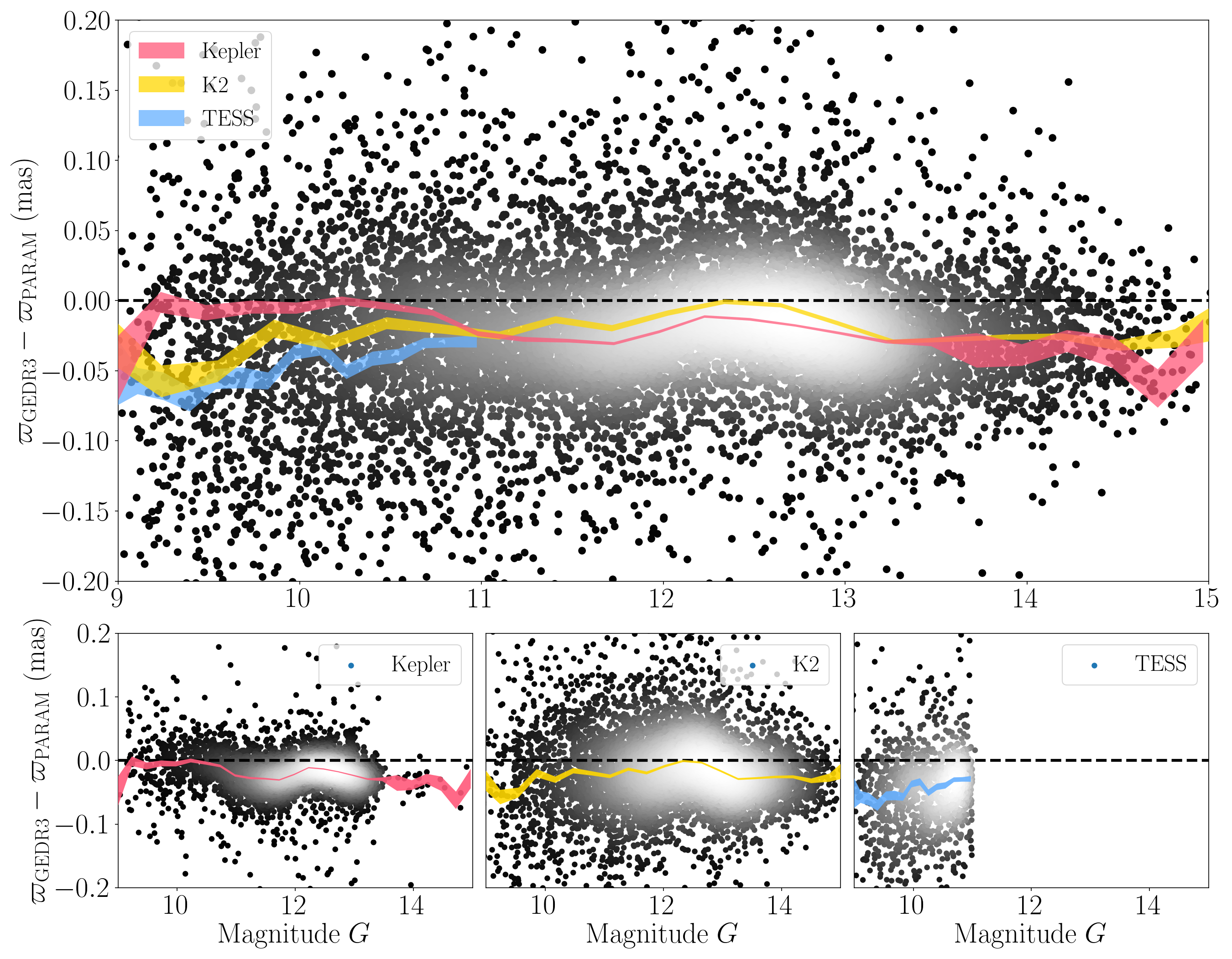
We investigate the parallax difference as a function of , and verify that is negative for all fields, in the sense that Gaia parallaxes are smaller (Fig. 2). We apply the same analysis as in K19 on the Kepler sample, but this time with Gaia EDR3 parallaxes and updated APOGEE constraints. shows fairly flat trends as a function of the ecliptic latitude, the effective wavenumber, the frequency of maximum oscillation, the mass inferred from PARAM, and the metallicity, but not for the magnitude which displays a non-linear feature (see bottom left panel of Fig. 2). This relation with is expected due to changes in the gating scheme or in the window size (see Fig. 17 in Fabricius et al. 2021). Despite the larger scatter and a higher proportion of fainter stars compared to Kepler, we also observe a non-linear trend as a function of if we combine all K2 fields together, which have an ecliptic latitude near zero (see bottom middle panel of Fig. 2). However, our TESS-SCVZ sample is too bright to see this trend.
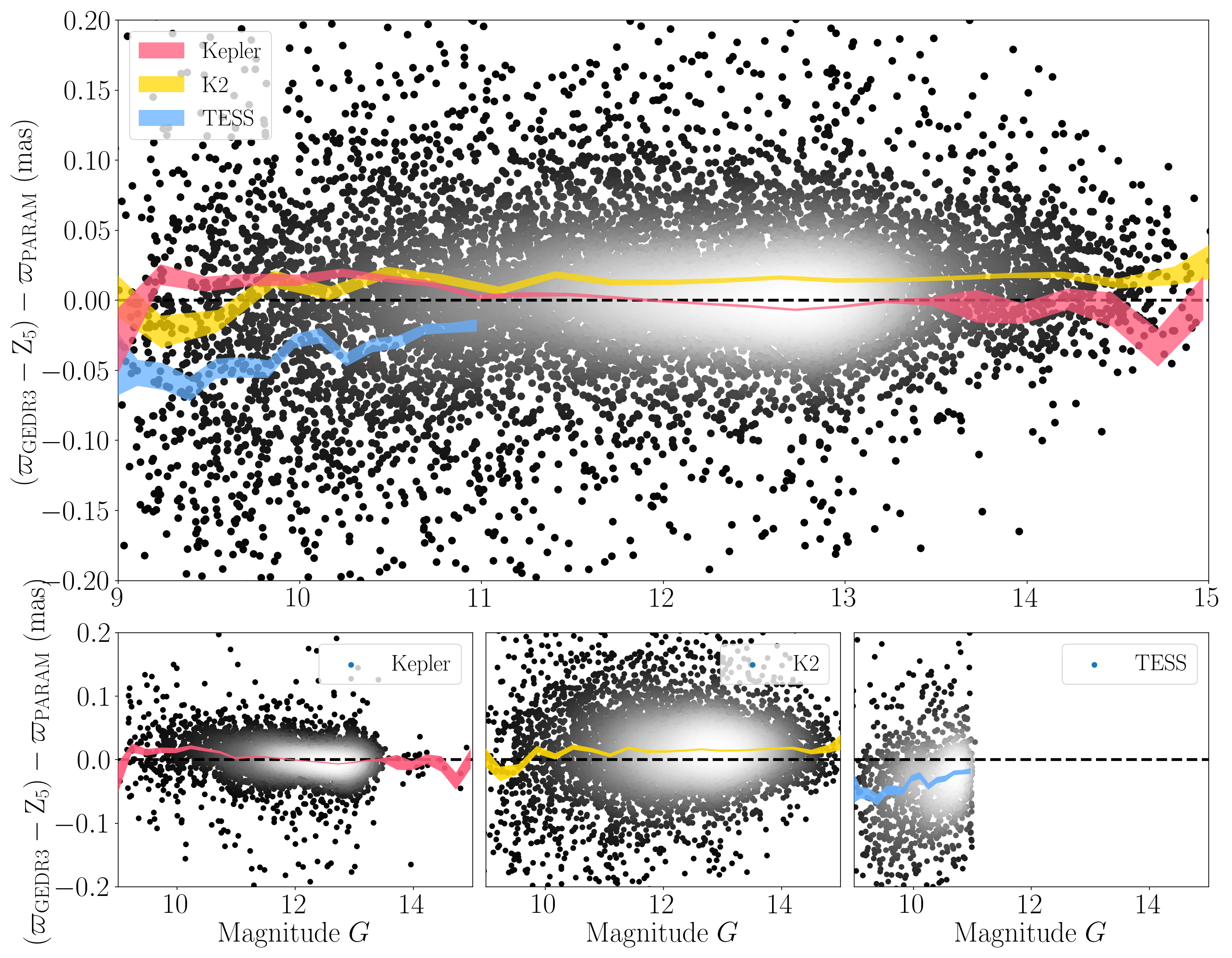
Figure 8 is similar to Fig. 2, but shows instead the parallax offset residuals , with -corrected Gaia EDR3 parallaxes. This removes the non-linear trend with . It is also clear from Fig. 8 that L21 corrections underestimate the parallax offset in the case of TESS, and overestimate it when it comes to K2 fields. But in Kepler, the residual parallax offset gets very close to zero. This suggests that L21 corrections are not universally suited for different types of sources, spanning a wide range of positions, magnitudes, and colours.
For some of the K2 campaigns (and independently of the spectroscopy used), we notice a significant trend of the parallax difference with the stellar mass. As we do not observe such a trend with mass for Kepler and TESS, we suspect that it could be related to, e.g., different noise levels in the various K2 campaigns. We tried using scaling relations to compute the mass and the asteroseismic parallax instead of PARAM, tested different asteroseismic pipelines and spectroscopic surveys, and removed high stars. Unfortunately, none of these made a difference and this is still being investigated (by BM and YE), as it might directly be related to the accuracy of seismically-inferred parameters.
4.2 A global picture
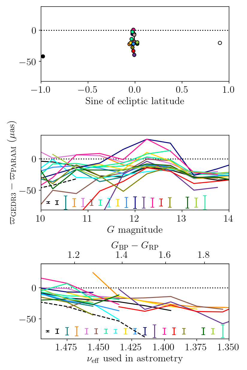
In Fig. 3, we show the offset estimates suggested from the difference between the uncorrected Gaia EDR3 and PARAM parallaxes, in the Kepler, the individual K2 campaigns, and the TESS-SCVZ fields. We analyse the relation between the parallax zero-point and the ecliptic latitude , the magnitude, and the effective wavenumber , which are the three parameters constituting the L21 correction model.
We first note that the offsets measured from asteroseismology either are close to zero or negative, and lie (at most) a few tens of as away from the zero-point suggested by quasars (). All the K2 campaigns have similar , close to zero, which is expected as the K2 survey observed solar-like oscillators all along the ecliptic.
For individual K2 campaigns, the parallax difference also follows a non-linear relation with , in line with what was discussed in Sec. 4.1. The bottom panel of Fig. 3 suggests that the parallax difference becomes more negative as we go towards lower , i.e. redder colours. This is also apparent for , where we have fewer campaigns. But one has to keep in mind that this trend is dominated by bright stars, for which other caveats exist (see e.g. Sec. 5.3), which tend to drag the parallax difference towards substantially negative values (as can be seen from the middle panel of Fig. 3).
5 Discussion
5.1 Magnitude of the red clump
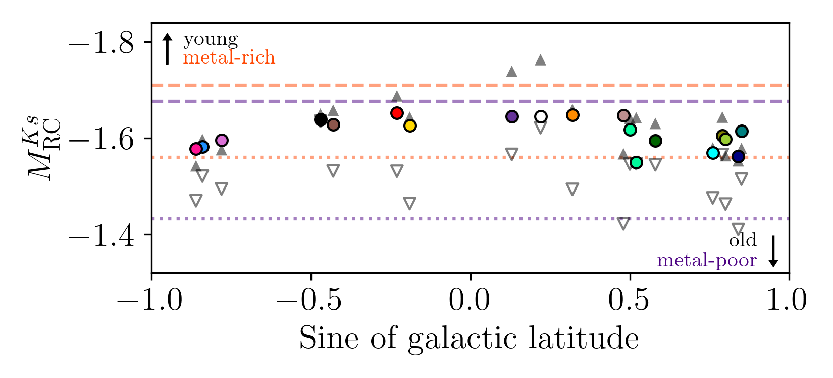
As a way to validate our findings, we also analyse the information provided by the magnitude of the red clump. In Fig. 4, we show different estimates of the absolute magnitude of the clump as a function of the galactic latitude . The first estimate is based on the -band absolute magnitude computed by PARAM, which is thus representative of our asteroseismic samples. For the other two estimates, we select Gaia EDR3 sources centred around the coordinates of each field and with : one estimate is calculated using the inverted Gaia uncorrected parallaxes, and the other with corrected parallaxes (using the L21 correction model). In order to be able to safely use inverted parallaxes, we restrict our samples to Gaia sources with a relative parallax uncertainty lower than 10%. Extinctions are calculated with the combined map (Marshall et al., 2006; Green et al., 2019; Drimmel et al., 2003) from mwdust444https://github.com/jobovy/mwdust (Bovy et al., 2016), and should only have a minor effect on the current analysis as we are working with -band magnitudes. For each dataset, we then compute the mode of the magnitude of the red clump using a Kernel Density Estimation with a fixed bandwidth (equal to 0.1) on the corresponding histogram.
The magnitude of the red clump shows a trend with the galactic latitude. Figure 3 of Ren et al. (2021) shows that the parallax offset is observed to be more negative for , which could explain why the filled triangles are more luminous in our Fig. 4. On the other hand, a brighter red clump luminosity would result from a younger and more metal-rich population. This trend is visible when using the seismic sample or the Gaia EDR3 sample without applying L21 parallax corrections. But the corrected Gaia EDR3 sample shows a flat trend instead, which again supports the idea that the L21 zero-point model is not suited to every kind of star (see also Sec. 4.1). In addition, results from asteroseismology agree well with model predictions (see e.g. Girardi, 2016).
5.2 Impact of Gaia scanning law statistics for K2
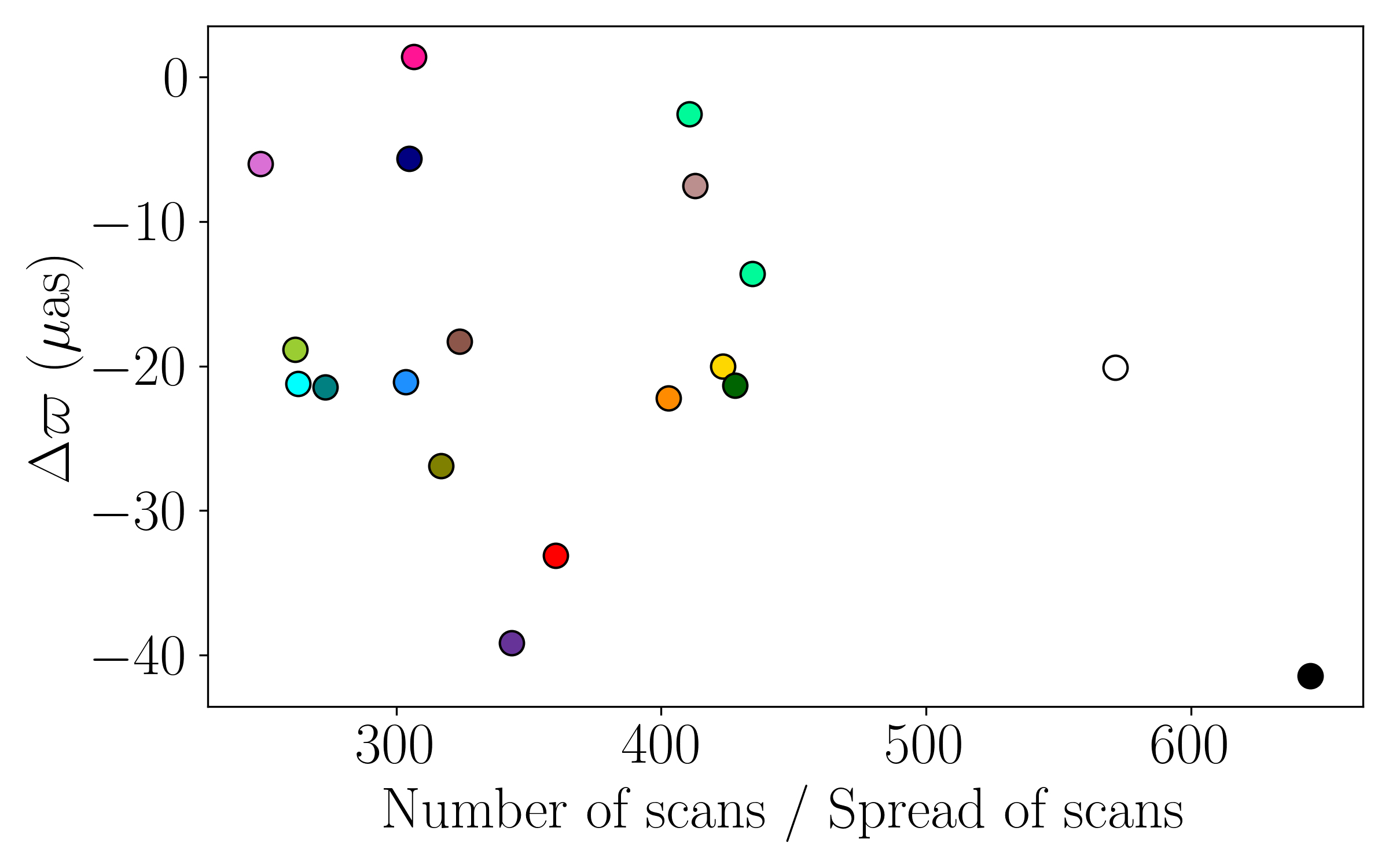
We look into whether the spread in parallax zero-points suggested by the K2 fields could be related to Gaia scan law statistics. For this, we extracted both the average number of scans and spread of scans throughout the year for Gaia EDR3 (see Fig. 1 of Everall et al., 2021, for the all-sky distribution of these quantities in Gaia DR2). The high ecliptic latitude fields, Kepler and TESS, show a high number of scans and an important spread of scans. On the other hand, for K2 we find fewer scans that are often concentrated at a single time of the year, which is consistent with the fact that these fields are located unfavourably with respect to the Gaia scanning law. As a result, the uncertainty on Gaia EDR3 parallaxes is larger for K2, compared to Kepler and TESS. Apart from these obvious differences, we do not observe any trend of the parallax offset with the scan law statistics, between the various K2 campaigns (see Fig. 5).
5.3 Existence of two magnitude regimes
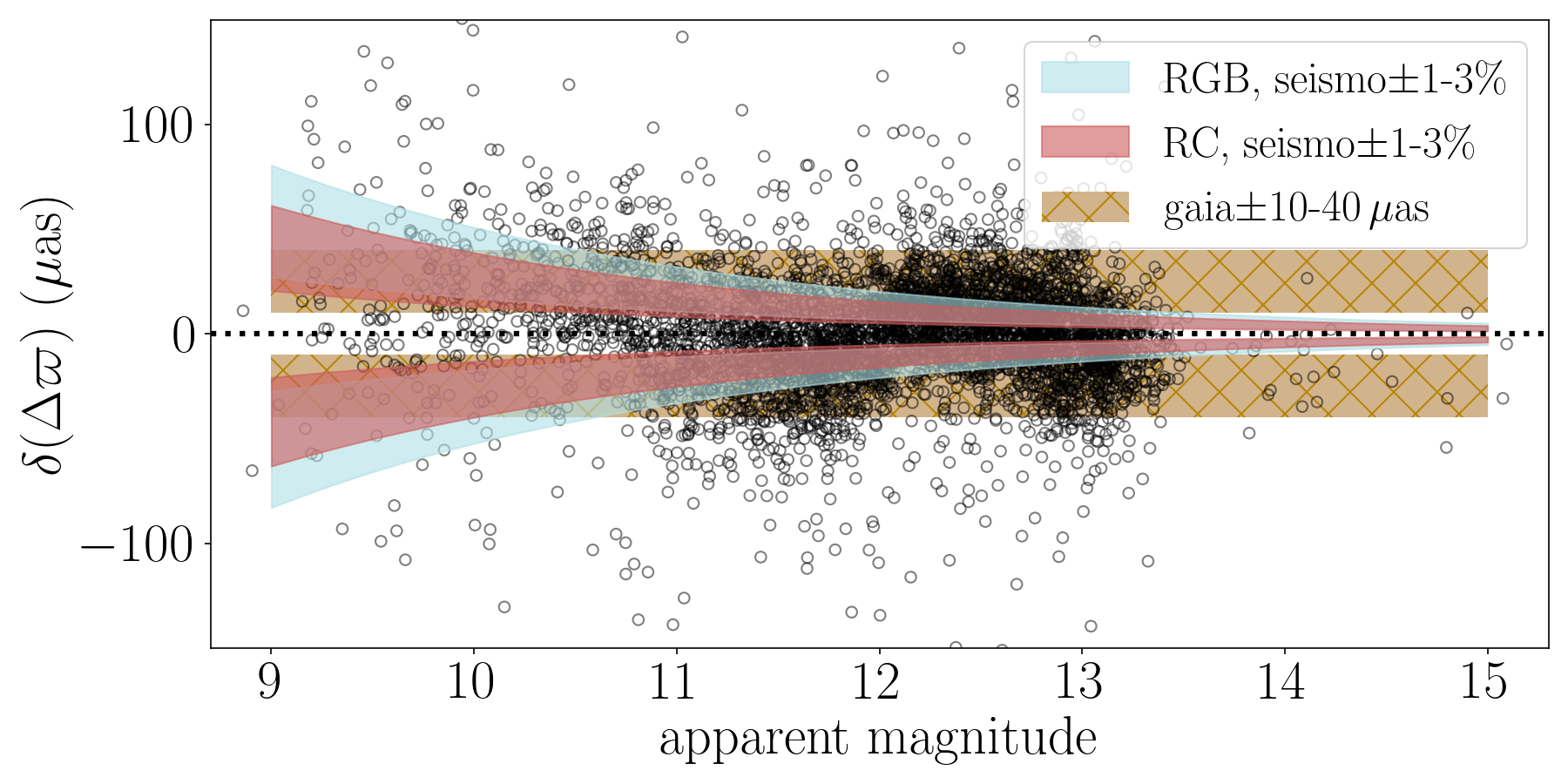
Figure 6 illustrates the biases arising from asteroseismology or Gaia’s side, as a function of the -band apparent magnitude. The asteroseismic bias corresponds to a fractional systematic uncertainty in radius, hence in distance; while the Gaia bias would be related to the effect of a systematic (absolute) uncertainty in parallax.
In order to test this, we consider two mock stars: one RGB star with , , [Fe/H] = 0.0 dex, , and a RC star with , , [Fe/H] = 0.0 dex, . We then estimate the absolute magnitude in -band. We consider a range of apparent magnitude values [9, 15], and compute a parallax value for each magnitude. ”Biased” parallaxes are then estimated: either adding a constant to the distance modulus, which would correspond to a fractional uncertainty in radius (asteroseismic bias); or adding a constant to the parallax itself (Gaia bias). For the former, we consider a 1-3% bias in radius, which corresponds to the 16th and 84th percentiles for the Kepler dataset; while for the latter, we use a range of -.
We show on Fig. 6 how such biases may affect the estimation of the parallax zero-point. The Kepler dataset is also shown in the background (after subtracting the mean parallax offset), to see how the order of magnitude of these biases compare with the actual observations. The existence of two regimes becomes quite clear: at the bright end, the comparisons in terms of parallax difference are dominated by systematics affecting the seismic parallax; and at the faint end, systematics from asteroseismology are much less dominant and one can potentially expose Gaia’s. This division stems from the fact that the fractional uncertainty on asteroseismic distances (or parallaxes) is largely distance independent, but the absolute precision (in pc or mas) is very much distance dependent, so it becomes worse than Gaia’s in nearby objects.
6 Conclusions
We carried out a follow-up of our 2019 study (Khan et al., 2019) to investigate the Gaia EDR3 parallax zero-point, for a significantly larger number of asteroseismic fields: Kepler, 17 K2 campaigns, and the TESS-SCVZ. Our analysis is similar to that of Zinn (2021) for the Kepler field but goes beyond with the addition of K2 and TESS, also making sure that we combine asteroseismic and spectroscopic constraints in a fully homogeneous way. This has the benefit of exploring Gaia parallax systematics for the same type of objects but with a wide range of positions over the sky within a single study. A quick comparison of asteroseismic distances with Gaia DR3’s GSP-Phot estimates shows that a reasonable agreement is found for objects within 2 kpc.
First, we confirm the positional dependence of the Gaia parallax zero-point: Kepler has an offset of as, K2 campaigns span a wide range between and as, and TESS shows an offset of as when using E20 and APOGEE constraints.
The inclusion of the Lindegren et al. (2021a) zero-point estimates improves the agreement between Gaia and asteroseismology in the case of Kepler and, to a much lesser extent, TESS. However, in most K2 fields, it can significantly over-correct the parallax difference, sometimes resulting in large positive parallax offsets. This underlines the need to consistently determine the parallax systematics applicable to the sample of interest, taking into account the distributions in position, magnitude, and colour. Such an over-correction had already been suggested by former studies (e.g. Bhardwaj et al., 2021; Riess et al., 2021).
Lastly, in terms of magnitude and colour dependence, we show that asteroseismology provides us with strong constraints on the Gaia EDR3 parallax zero-point, in ranges that are not necessarily well-sampled by L21 corrections. There are no clear trends with the ecliptic latitude or the magnitude, but the zero-point values tend to increase (in absolute terms) towards redder colours (lower ). Although this trend seems to be dominated by caveats associated with stars at brighter magnitudes. Moreover, we find that seismic-based estimates of the red clump magnitude are consistent with theoretical predictions of , and that the inclusion of the L21 offset tends to make the red clump too faint. We do not find any correlation between Gaia scan law statistics and parallax offset estimates for the K2 fields. We also use two mock stars to illustrate the existence of two regimes: bright magnitudes, where Gaia’s precision is better than asteroseismology’s; and faint magnitudes, where we can expose Gaia’s limits thanks to seismology’s precision.
With this study, we present asteroseismology as a powerful tool for constraining Gaia systematics. Red giants come with several benefits: they are single stars with measurable parallaxes and without large-amplitude photometric variations, and consequently differ substantially from eclipsing binaries, quasars, RR Lyrae and Cepheids. Further progress is foreseen with Gaia DR4 which will have improved parallax uncertainties and reduced systematics. And, in a forthcoming paper, we will look in more detail at the uncertainties potentially affecting parallax estimates from asteroseismology and Gaia, and see how we can define the best sample to investigate parallax systematics in Gaia.
Acknowledgements.
This work has made use of data from the European Space Agency (ESA) mission Gaia (https://www.cosmos.esa.int/gaia), processed by the Gaia Data Processing and Analysis Consortium (DPAC, https://www.cosmos.esa.int/web/gaia/dpac/consortium). Funding for the DPAC has been provided by national institutions, in particular the institutions participating in the Gaia Multilateral Agreement. RIA and SK are funded by the Swiss National Science Foundation (SNSF) through an Eccellenza Professorial Fellowship (award PCEFP2_194638). AM and EW acknowledge support from the ERC Consolidator Grant funding scheme (project ASTEROCHRONOMETRY, G.A. n. 772293). This research was supported by the International Space Science Institute (ISSI) in Bern, through ISSI International Team project #490, SHoT: The Stellar Path to the Ho Tension in the Gaia, TESS, LSST and JWST Era.References
- Abdurro’uf et al. (2022) Abdurro’uf, Accetta, K., Aerts, C., et al. 2022, ApJS, 259, 35
- Bhardwaj et al. (2021) Bhardwaj, A., Rejkuba, M., de Grijs, R., et al. 2021, ApJ, 909, 200
- Borucki et al. (2010) Borucki, W. J., Koch, D., Basri, G., et al. 2010, Science, 327, 977
- Bovy et al. (2016) Bovy, J., Rix, H.-W., Green, G. M., Schlafly, E. F., & Finkbeiner, D. P. 2016, ApJ, 818, 130
- Buder et al. (2021) Buder, S., Sharma, S., Kos, J., et al. 2021, MNRAS, 506, 150
- Cardelli et al. (1989) Cardelli, J. A., Clayton, G. C., & Mathis, J. S. 1989, ApJ, 345, 245
- Cruz Reyes & Anderson (2023) Cruz Reyes, M. & Anderson, R. I. 2023, A&A, 672, A85
- Drimmel et al. (2003) Drimmel, R., Cabrera-Lavers, A., & López-Corredoira, M. 2003, A&A, 409, 205
- Elsworth et al. (2017) Elsworth, Y., Hekker, S., Basu, S., & Davies, G. R. 2017, MNRAS, 466, 3344
- Elsworth et al. (2020) Elsworth, Y., Themeßl, N., Hekker, S., & Chaplin, W. 2020, Research Notes of the American Astronomical Society, 4, 177
- Everall et al. (2021) Everall, A., Boubert, D., Koposov, S. E., Smith, L., & Holl, B. 2021, MNRAS, 502, 1908
- Fabricius et al. (2021) Fabricius, C., Luri, X., Arenou, F., et al. 2021, A&A, 649, A5
- Fouesneau et al. (2022) Fouesneau, M., Frémat, Y., Andrae, R., et al. 2022, arXiv e-prints, arXiv:2206.05992
- Gaia Collaboration et al. (2021) Gaia Collaboration, Brown, A. G. A., Vallenari, A., et al. 2021, A&A, 649, A1
- Gaia Collaboration et al. (2022) Gaia Collaboration, Vallenari, A., Brown, A. G. A., et al. 2022, arXiv e-prints, arXiv:2208.00211
- Girardi (2016) Girardi, L. 2016, Annual Review of Astronomy and Astrophysics, 54, 95
- Girardi et al. (2002) Girardi, L., Bertelli, G., Bressan, A., et al. 2002, A&A, 391, 195
- Green et al. (2019) Green, G. M., Schlafly, E., Zucker, C., Speagle, J. S., & Finkbeiner, D. 2019, ApJ, 887, 93
- Howell et al. (2014) Howell, S. B., Sobeck, C., Haas, M., et al. 2014, PASP, 126, 398
- Huang et al. (2021) Huang, Y., Yuan, H., Beers, T. C., & Zhang, H. 2021, ApJ, 910, L5
- Khan et al. (2019) Khan, S., Miglio, A., Mosser, B., et al. 2019, A&A, 628, A35
- Lindegren et al. (2021a) Lindegren, L., Bastian, U., Biermann, M., et al. 2021a, A&A, 649, A4
- Lindegren et al. (2021b) Lindegren, L., Klioner, S. A., Hernández, J., et al. 2021b, A&A, 649, A2
- Mackereth et al. (2021) Mackereth, J. T., Miglio, A., Elsworth, Y., et al. 2021, MNRAS, 502, 1947
- Marshall et al. (2006) Marshall, D. J., Robin, A. C., Reylé, C., Schultheis, M., & Picaud, S. 2006, A&A, 453, 635
- Miglio et al. (2021) Miglio, A., Chiappini, C., Mackereth, J. T., et al. 2021, A&A, 645, A85
- Molinaro et al. (2023) Molinaro, R., Ripepi, V., Marconi, M., et al. 2023, MNRAS, 520, 4154
- Mosser & Appourchaux (2009) Mosser, B. & Appourchaux, T. 2009, A&A, 508, 877
- O’Donnell (1994) O’Donnell, J. E. 1994, ApJ, 422, 158
- Ren et al. (2021) Ren, F., Chen, X., Zhang, H., et al. 2021, ApJ, 911, L20
- Ricker et al. (2015) Ricker, G. R., Winn, J. N., Vanderspek, R., et al. 2015, Journal of Astronomical Telescopes, Instruments, and Systems, 1, 014003
- Riess et al. (2021) Riess, A. G., Casertano, S., Yuan, W., et al. 2021, ApJ, 908, L6
- Rodrigues et al. (2017) Rodrigues, T. S., Bossini, D., Miglio, A., et al. 2017, MNRAS, 467, 1433
- Stassun & Torres (2021) Stassun, K. G. & Torres, G. 2021, ApJ, 907, L33
- Zinn (2021) Zinn, J. C. 2021, AJ, 161, 214
Appendix A Catalogues of asteroseismic, spectroscopic, and astrometric properties for Kepler, K2, and TESS red giants
| Column Identifier | Description | Units |
|---|---|---|
| KIC/K2_ID/TIC | Kepler/K2/TESS ID | |
| K2_campaign | K2 campaign number | |
| GEDR3_source_id | Gaia EDR3 source id | |
| GEDR3_ra | Gaia EDR3 right ascension | |
| GEDR3_dec | Gaia EDR3 declination | |
| GEDR3_l | Gaia EDR3 galactic longitude | |
| GEDR3_b | Gaia EDR3 galactic latitude | |
| GEDR3_ecl_lon | Gaia EDR3 ecliptic longitude | |
| GEDR3_ecl_lat | Gaia EDR3 ecliptic latitude | |
| GEDR3_parallax | Gaia EDR3 parallax | |
| GEDR3_parallax_Z5 | L21 correction (5p) | |
| GEDR3_phot_g_mean_mag | Gaia EDR3 -band magnitude | |
| GEDR3_phot_bp_mean_mag | Gaia EDR3 -band magnitude | |
| GEDR3_phot_rp_mean_mag | Gaia EDR3 -band magnitude | |
| GEDR3_nu_eff_used_in_astrometry | Gaia EDR3 effective wavenumber | |
| GEDR3_pseudocolour | Gaia EDR3 pseudocolour | |
| GEDR3_astrometric_params_solved | Gaia EDR3 number of astrometric parameters solved | |
| GEDR3_ruwe | Gaia EDR3 renormalised unit weight error | |
| GEDR3_ipd_frac_multi_peak | Gaia EDR3 percent of successful-IPD windows with more than one peak | |
| GEDR3_ipd_gof_harmonic_amplitude | Gaia EDR3 amplitude of the IPD GoF versus position angle of scan | |
| GDR3_non_single_star | Gaia DR3 flag indicating the availability in Non-Single Star tables | |
| GDR3_distance_gspphot | Gaia DR3 distance from GSP-Phot | |
| GDR3_ag_gspphot | Gaia DR3 extinction in -band from GSP-Phot | |
| 2MASS_kmag | 2MASS -band magnitude | |
| APOGEE_ID | APOGEE ID | |
| APOGEE_teff | APOGEE | |
| APOGEE_feh | APOGEE | |
| APOGEE_alpha | APOGEE | |
| APOGEE_mh | APOGEE | |
| APOGEE_ASPCAPFLAGS | APOGEE flag for issues associated with the ASPCAP fits | |
| GALAH_teff | GALAH | |
| GALAH_feh | GALAH | |
| GALAH_alpha | GALAH | |
| GALAH_mh | GALAH | |
| GALAH_flag_sp | GALAH stellar parameter quality flag | |
| GALAH_flag_fe_h | GALAH quality flag | |
| GALAH_flag_alpha_fe | GALAH quality flag | |
| MA09_numax | from MA09 pipeline | |
| MA09_Dnu | from MA09 pipeline | |
| MA09_PARAM_mass | Mass from PARAM, based on MA09 and APOGEE/GALAH | |
| MA09_PARAM_rad | Radius from PARAM, based on MA09 and APOGEE/GALAH | |
| MA09_PARAM_mbol | Bolometric magnitude from PARAM, based on MA09 and APOGEE/GALAH | |
| MA09_PARAM_dist | Distance from PARAM, based on MA09 and APOGEE/GALAH | |
| MA09_PARAM_Av | Visual extinction from PARAM, based on MA09 and APOGEE/GALAH | |
| MA09_PARAM_Ks | absolute magnitude from PARAM, based on MA09 and APOGEE/GALAH | |
| MA09_PARAM_parallax | Parallax from PARAM, based on MA09 and APOGEE/GALAH | |
| E20_numax | from E20 pipeline | |
| E20_Dnu | from E20 pipeline | |
| E20_PARAM_mass | Mass from PARAM, based on E20 and APOGEE/GALAH | |
| E20_PARAM_rad | Radius from PARAM, based on E20 and APOGEE/GALAH | |
| E20_PARAM_mbol | Bolometric magnitude from PARAM, based on E20 and APOGEE/GALAH | |
| E20_PARAM_dist | Distance from PARAM, based on E20 and APOGEE/GALAH | |
| E20_PARAM_Av | Visual extinction from PARAM, based on E20 and APOGEE/GALAH | |
| E20_PARAM_Ks | absolute magnitude from PARAM, based on E20 and APOGEE/GALAH | |
| E20_PARAM_parallax | Parallax from PARAM, based on E20 and APOGEE/GALAH | |
| E17_evstate | Elsworth et al. (2017) evolutionary state |
Appendix B Comparison with Gaia DR3 Apsis GSP-Phot distances
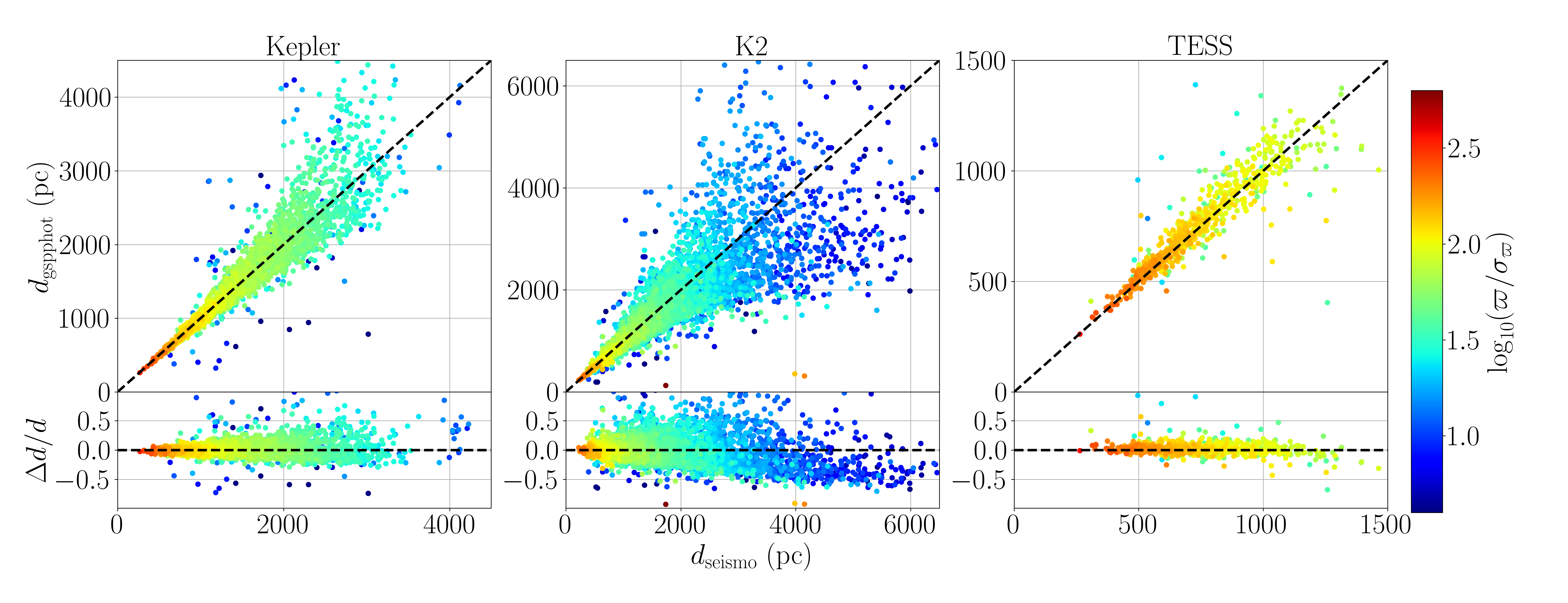
Figure 7 compares distances from asteroseismology (based on E20 and APOGEE) and Gaia DR3 Apsis GSP-Phot for Kepler, K2, and TESS. As noted by Fouesneau et al. (2022), a good agreement is found to about 2 kpc; beyond, GSP-Phot tends to overestimate distances as in Kepler, or on the contrary to systematically underestimate them at even further distances (see K2). No issues are found for TESS nearby targets.
Appendix C Parallax zero-point estimates from asteroseismology
Table 4 gives a summary of the parallax offsets measured with the various combinations of asteroseismology and spectroscopy in the Kepler, K2 campaigns, and TESS fields.
| Field | MA09+APOGEE | E20+APOGEE * | MA09+GALAH | E20+GALAH |
|---|---|---|---|---|
| Kepler | (4687) | (4687) | - | - |
| K2 C01 | (201) | (201) | (240) | (240) |
| K2 C02 | (386) | (386) | (620) | (620) |
| K2 C03 | (543) | (543) | (262) | (262) |
| K2 C04 | (1092) | (1092) | (474) | (474) |
| K2 C05 | (865) | (865) | (757) | (757) |
| K2 C06 | (690) | (690) | (262) | (262) |
| K2 C07 | (422) | (422) | (822) | (822) |
| K2 C08 | (436) | (436) | (159) | (159) |
| K2 C10 | (199) | (199) | (117) | (117) |
| K2 C11 | (189) | (189) | (235) | (235) |
| K2 C12 | (462) | (462) | (63) | (63) |
| K2 C13 | (423) | (423) | (645) | (645) |
| K2 C14 | (354) | (354) | (123) | (125) |
| K2 C15 | (10) | (10) | (735) | (735) |
| K2 C16 | (310) | (310) | (201) | (201) |
| K2 C17 | (348) | (348) | (162) | (162) |
| K2 C18 | (94) | (94) | (78) | (78) |
| TESS | (1253) | (1253) | - | - |
Appendix D Impact of L21 corrections on parallax offset estimation