Ledoit-Wolf linear shrinkage with unknown mean

Abstract

This work addresses large dimensional covariance matrix estimation with unknown mean. The empirical covariance estimator fails when dimension and number of samples are proportional and tend to infinity, settings known as Kolmogorov asymptotics. When the mean is known, Ledoit and Wolf (2004) proposed a linear shrinkage estimator and proved its convergence under those asymptotics. To the best of our knowledge, no formal proof has been proposed when the mean is unknown. To address this issue, we propose a new estimator and prove its quadratic convergence under the Ledoit and Wolf assumptions. Finally, we show empirically that it outperforms other standard estimators.

Keywords: covariance matrix estimation, linear shrinkage, Ledoit-Wolf estimator, unknown mean, general asymptotics

Declarations of interest: none

1 Introduction and related work

The covariance matrix plays a major role in numerous machine learning algorithms and statistics. Just to cite a few, the PCA [1] in machine learning, Markowitz portfolio management [2] in finance, or generalized method of moments estimators [3] in statistics. However, those algorithms are designed to use the true covariance matrix, which is often unaccessible. Even if the sample covariance matrix seems to be a simple and appealing choice, it severely fails in many applications: for instance, the use of the sample covariance matrix for Markowitz portfolio management does not beat a naive uniform distribution among the assets [4].

In the context of Kolmogorov asymptotics, where the ratio of the dimension $p_{n}$ and the number of samples $n$ tends to a finite positive constant $\frac{p_{n}}{n}\rightarrow c>0$, this estimator fails to converge quadratically. Moreover, its eigenvalue spectrum is biased: high eigenvalues tends at being too high, and low ones, too low. The behavior of the eigenvalues is studied in random matrix theory: in the context of the Kolmogorov asymptotics, this topic is widely covered by V. L. Girko [5, 6, 7].

We focus on the shrinkage-type estimators which have suitable asymptotic properties, influenced by the work of Stein on Gaussian mean estimation in 1956 [8]. Due to their simplicity to implement and strong theoretical support, linear methods are widely used, and, for some, implemented in ScikitLearn [9]: Ledoit-Wolf linear shrinkage [10], which will be our main focus, its extension for Gaussian distributions using Rao-Blackwell theorem, named Oracle Approximating Shrinkage (OAS) estimator [11], linear shrinkage with factor models [12], linear shrinkage for elliptical distributions with unknown mean and known radius distribution [13], just to name a few. Non-linear methods propose shrinkage methods where the factor differs from an eigenvalue to an other. Among them, Stein’s covariance estimator [14] works for Gaussian distributions, and several algorithms were developed by Ledoit and Wolf using eigenvalue spectrum analysis from random matrix theory [15, 16, 17]. Further theoretical analysis of those algorithms can be found in [18, 19, 20].

Usually, when estimating the covariance matrix, we don’t know the mean of the distribution. Yet, the extension from known to unknown mean is rarely studied. To extend the empirical covariance with $T$ samples $S_{T}$, one uses the unbiased estimator $\tilde{S}_{T}$, after removing the empirical mean and dividing by $T-1$ instead of $T$. If it seems straightforward for $S_{T}$, it can be non trivial for more complex estimators. Ahurbekova explicitly worked in the case of known then unknown mean [13], and the resulting estimators of linear shrinkage for elliptical distributions with known radius distributions are notably different from the ones with a known mean. In the review of their work in 2020 [21], Ledoit and Wolf worked and proved their results in the case where the mean is known, and they claim at the end ”One then simply replaces $S_{T}$ with $\tilde{S}_{T}$ and $T$ with $T–1$ in all the previous descriptions and computations in practice” (Section 6: Computational Aspects and Code). However, to the best of our knowledge, there are no proofs in the literature to extend the theoretical results, nor show the optimality of this approach. Moreover, focusing on Ledoit-Wolf linear shrinkage algorithm, one can note that the implementation used in ScikitLearn [9] doesn’t follow the recommendations of Ledoit and Wolf regarding the case of uncentered data. They didn’t change $T$ to $T-1$ and used $\frac{T-1}{T}\tilde{S}_{T}$ instead of $\tilde{S}_{T}$. Unexpectedly, experiments show notably worse results using Ledoit and Wolf recommendations rather than the ScikitLearn implementation. This remark underlines that the problem is more counter-intuitive than expected, and a closer look at the dependence between the covariance and the mean estimation is required.

We address the lack of theoretical results when the mean is unknown and propose a new Ledoit-Wolf-like linear shrinkage estimator and its theoretical and empirical analysis.

2 Notations, definitions and hypotheses

Let us introduce the following notations.

Notation 1.

In the following we consider a sequence of observation matrices $(X_{n})_{n\in\mathbb{N}^{*}}$ with $X_{n}\in\mathbb{R}^{p_{n}\times n}$ of $n$ iid observations on a system of $p_{n}$ dimensions. Decomposing the covariance matrix, we denote $\Sigma_{n}=\Gamma_{n}\Lambda_{n}\Gamma_{n}^{t}$, where $\Lambda_{n}$ is a diagonal matrix and $\Gamma_{n}$ a rotation matrix. The diagonal elements of $\Lambda_{n}$ are the eigenvalues $\lambda_{1}^{n},...,\lambda_{p_{n}}^{n}$, and the columns of $\Gamma_{n}$ are the eigenvectors $\gamma_{1}^{n},...,\gamma_{p_{n}}^{n}$. $Y_{n}=\Gamma_{n}^{t}X_{n}$ is a $p_{n}\times n$ matrix of $n$ iid observations of $p_{n}$ uncorrelated random variables $(y_{1}^{n},...,y_{n}^{n})$.

Notation 2.

Let $A_{n}$ and $B_{n}$ two $p_{n}\times p_{n}$ matrices. We consider the Frobenius norm: $\lVert A_{n}\rVert=\sqrt{\tr(A_{n}A_{n}^{t})/p_{n}}$, and the associated inner product: $\langle A_{n},B_{n}\rangle_{n}=\tr(A_{n}B_{n}^{t})/p_{n}$. Dividing by the dimension is not standard, it is done to fix the norm of the identity as $1$ regardless of the dimension.

Notation 3.

Let $(E_{n})_{n}$ a sequence of euclidean spaces with associated norm $\lVert\cdot\rVert_{n}$. The quadratic convergence of a random variable $Z_{n}\in E_{n}$, i.e. $\mathbb{E}[\lVert Z_{n}\rVert_{n}^{2}]\rightarrow 0$, is denoted as $Z_{n}\underset{q.m}{\longrightarrow}0$.

We describe now several assumptions, the same used in the linear shrinkage of Ledoit and Wolf [10], that will be used in the following.

Assumption 1.

There exists a constant $K_{1}$ independent of $n$ such that $p_{n}/n\leq K_{1}$.

Assumption 2.

There exists a constant $K_{2}$ independent of $n$ such that $\frac{1}{p_{n}}\sum_{i=1}^{p_{n}}\mathbb{E}\left[(\tilde{y}_{i1}^{n})^{8}\right]\leq K_{2}$ where for all $i\in\llbracket 1,p_{n}\rrbracket$, $\tilde{y}_{i1}^{n}=y_{i1}^{n}-\mathbb{E}[y_{i1}^{n}]$.

Assumption 3.

$$\lim_{n\rightarrow\infty}\frac{p_{n}^{2}}{n}\times\frac{\sum_{(i,j,k,l)\in Q_{n}}(\text{Cov}[\tilde{y}_{i1}^{n}\tilde{y}_{j1}^{n},\tilde{y}_{k1}^{n}\tilde{y}_{l1}^{n}])^{2}}{|Q_{n}|}=0,$$

where $Q_{n}$ denotes the set of all the quadruples that are made of four distinct integers between $1$ and $p_{n}$, and for all $i\in\llbracket 1,p_{n}\rrbracket$, $\tilde{y}_{i1}^{n}=y_{i1}^{n}-\mathbb{E}[y_{i1}^{n}]$.

We need some definitions to properly define the problem and the asymptotics.

Definition 1 (Empirical covariance).

For an observation matrix $X_{n}$ of size $p_{n}\times n$, we define the empirical covariance as:

$$S_{n}=\tilde{X}_{n}\tilde{X}_{n}^{t}/(n-1),$$

with $(\tilde{X}_{n})_{ik}=(X_{n})_{ik}-\frac{1}{n}\sum_{k^{\prime}=1}^{n}(X_{n})_{ik^{\prime}}$.

Definition 2 (Scalars $(\mu_{n},\alpha_{n}^{2},\beta_{n}^{2},\delta_{n}^{2})$).

We define four scalars:

$$\mu_{n}=\langle\Sigma_{n},I_{p_{n}}\rangle_{n},\alpha_{n}^{2}=\lVert\Sigma_{n}-\mu_{n}I_{p_{n}}\rVert_{n}^{2},\beta_{n}^{2}=\mathbb{E}[\lVert S_{n}-\Sigma_{n}\rVert_{n}^{2}],\delta_{n}^{2}=\mathbb{E}[\lVert S_{n}-\mu_{n}I_{p_{n}}\rVert_{n}^{2}].$$

(Lemma 2.1 in (Ledoit and Wolf, 2004) [10]) proves that $\alpha_{n}^{2}+\beta_{n}^{2}=\delta_{n}^{2}$.

The oracle linear shrinkage estimator is given by the following minimization problem. The following corollary is the central point of the linear shrinkage methods.

Corollary 1 (Corollary of theorem 2.1 from (Ledoit and Wolf, 2004)).

Consider the optimization problem:

$$\operatorname*{minimize}_{\begin{subarray}{c}\rho_{1},\rho_{2}\\ \text{s.t. }\Sigma_{n}^{*}=\rho_{1}I_{p_{n}}+\rho_{2}S_{n}\end{subarray}}\mathbb{E}[\lVert\Sigma_{n}^{*}-\Sigma_{n}\rVert_{n}^{2}],$$

where the coefficients $\rho_{1}$ and $\rho_{2}$ are not random. Its solution $\Sigma_{n}^{*}$ verifies:

$$\Sigma_{n}^{*}=\frac{\beta_{n}^{2}}{\delta_{n}^{2}}\mu_{n}I_{p_{n}}+\frac{\alpha_{n}^{2}}{\delta_{n}^{2}}S_{n},\quad\mathbb{E}[\lVert\Sigma_{n}^{*}-\Sigma_{n}\rVert_{n}^{2}]=\frac{\alpha_{n}^{2}\beta_{n}^{2}}{\delta_{n}^{2}}.$$

Remark 1.

Corollary 1 remains true for any unbiased estimator $\hat{\Sigma}_{n}$ instead of $S_{n}$.

$(\mu_{n},\alpha_{n}^{2},\beta_{n}^{2},\delta_{n}^{2})$ depends on the true covariance $\Sigma_{n}$, and thus can’t be used directly in the estimation of $\Sigma_{n}^{*}$. The central issue of this work is to find estimators $(m_{n},a_{n}^{2},b_{n}^{2},d_{n}^{2})$ of $(\mu_{n},\alpha_{n}^{2},\beta_{n}^{2},\delta_{n}^{2})$ in order to compute an estimation $S_{n}^{*}$ of $\Sigma_{n}^{*}$. As the mean is unknown, those estimators differ from Ledoit and Wolf work [10], particularly when $p_{n}$ is higher than $n$.

3 Theoretical results

All the following results extend the work of Ledoit and Wolf [10] in the case where the empirical mean is used as estimator of the mean.
All proofs are shown in appendix A.

Remark 2.

In the following, as all the estimators are invariant by change of mean, resulting from the definition of $\tilde{X}=X-\sum_{k}X_{\cdot,k}$, we can assume $\mathbb{E}[X]=0$ for the simplicity of notations.

We present a sequence of lemmata, that naturally define estimators with suitable asymptotic properties for the scalars $(\mu_{n},\alpha_{n}^{2},\beta_{n}^{2},\delta_{n}^{2})$.

Lemma 1.

Under assumptions 1 and 2, $\mu_{n},\alpha_{n}^{2},\beta_{n}^{2},\delta_{n}^{2}$ remain bounded as $n\rightarrow\infty$.

Theorem 1.

Under assumptions 1 and 2, define $\theta_{n}^{2}=\mathbb{V}\left[\frac{1}{p_{n}}\sum_{i=1}^{p_{n}}(y_{i1}^{n})^{2}]\right]$. $\theta_{n}^{2}$ is bounded as $n\rightarrow\infty$, and we have:

$$\lim_{n\rightarrow\infty}\mathbb{E}[\lVert S_{n}-\Sigma_{n}\rVert_{n}^{2}]-\frac{p_{n}}{n}(\mu_{n}^{2}+\theta_{n}^{2})=0.$$

In particular, taking $p_{n}=p$ constant, we see that $S_{n}\underset{q.m}{\longrightarrow}\Sigma_{n}$. But, when $p_{n}$ is of the same order of magnitude than $n$, the sample covariance generally fails to converge as the error is at least of the same order of magnitude as $\mu_{n}^{2}=\langle\Sigma_{n},I_{p_{n}}\rangle_{n}^{2}$.

Lemma 2 (Estimator of $\mu_{n}$).

Define $m_{n}=\langle S_{n},I_{p_{n}}\rangle_{n}$. Then, under assumptions 1 and 2, $\mathbb{E}[m_{n}]=\mu_{n}$ for all $n$, and $m_{n}-\mu_{n}$ converges to zero in quartic mean (fourth moment) as $n$ goes to infinity.

Corollary 2.

Under assumptions 1 and 2, $m_{n}^{2}-\mathbb{E}[m_{n}^{2}]$ converges to zero in quadratic mean as $n$ goes to infinity.

Lemma 3 (Estimator of $\delta_{n}^{2}$).

Define $d_{n}^{2}=\lVert S_{n}-m_{n}I_{p_{n}}\rVert_{n}^{2}$. Then, under assumptions 1, 2 and 3, $d_{n}^{2}-\delta_{n}^{2}\underset{q.m}{\longrightarrow}0$. It follows that $d_{n}^{2}-\mathbb{E}[d_{n}^{2}]\underset{q.m}{\longrightarrow}0$.

The following lemmata aim at defining an unbiased estimator of $\beta_{n}^{2}$ that quadratically converges. We work around $\bar{b}_{n}^{2}$, inspired from the estimator of $\beta_{n}^{2}$ in the case where the mean is known, and write residual terms in the expectation as a combination of $m_{n}$ and $d_{n}^{2}$.

Lemma 4.

Define:

$$\bar{b}_{n}^{2}=\frac{1}{n^{2}}\sum_{k=1}^{n}\left\lVert\frac{n}{n-1}\tilde{x}_{\cdot k}^{n}(\tilde{x}_{\cdot k}^{n})^{t}-S_{n}\right\rVert_{n}^{2},$$

where $\tilde{x}_{\cdot k}^{n}=x_{\cdot k}^{n}-\frac{1}{n}\sum_{k^{\prime}=1}^{n}x_{\cdot k^{\prime}}^{n}$ and $(x_{\cdot 1}^{n},...,x_{\cdot k}^{n},...,x_{\cdot n}^{n})$ are the independent samples forming $X$. Then, under assumption 1,

$$\mathbb{E}[\bar{b}_{n}^{2}]=c_{0}\beta_{n}^{2}+c_{1}\delta_{n}^{2}+c_{2}\mu_{n}^{2},$$

with $\gamma_{n}=\frac{n(n-1)}{n^{2}-3n+3},\lambda_{n}=\frac{n^{2}(n-2)}{(n-1)(n^{2}-3n+3)},c_{0}=\frac{1}{\gamma_{n}}-\frac{1}{n}-\frac{\lambda_{n}}{\gamma_{n}n^{2}},c_{1}=\frac{\lambda_{n}}{\gamma_{n}n^{2}},c_{2}=(p+1)c_{1}$.

Lemma 5.

Under assumption 1, we have: $\mathbb{E}[\bar{b}_{n}^{2}]=c_{0}\beta_{n}^{2}+c_{1}\mathbb{E}[d_{n}^{2}]+c_{2}\mathbb{E}[m_{n}^{2}]+(c_{1}-c_{2})\mathbb{V}[m_{n}]$.

Lemma 6.

Under assumption 1, we have: $\mathbb{V}[\bar{b}_{n}^{2}]\underset{n\rightarrow\infty}{\longrightarrow}0$.

We need to compute $\mathbb{V}[m_{n}]$ which is unknown in the development of $\mathbb{E}[\bar{b}_{n}^{2}]$ in Lemma 5.

Lemma 7.

Under assumption 1, we have: $\mathbb{V}[m_{n}]=q_{0}\beta_{n}^{2}+q_{1}\delta_{n}^{2}-q_{2}\mu_{n}^{2}$,
with $q_{0}=\frac{n-2}{p(n-1)},q_{1}=\frac{1}{p(n-1)},q_{2}=\frac{p-1}{p(n-1)}$.

Lemma 8.

Under assumption 1, we have: $\mathbb{V}[m_{n}]=\frac{1}{1-q_{1}-q_{2}}\left(q_{0}\beta_{n}^{2}+q_{1}\mathbb{E}[d_{n}^{2}]-q_{2}\mathbb{E}[m_{n}^{2}]\right)$.

Lemma 9.

Define:

$$b_{n}^{2}=\frac{1}{c_{0}^{f}}\left(\bar{b}_{n}^{2}-c_{1}^{f}d_{n}^{2}-c_{2}^{f}m_{n}^{2}\right),$$

with $c_{0}^{f}=c_{0}+(c_{1}-c_{2})\frac{q_{0}}{1-q_{1}-q_{2}},c_{1}^{f}=c_{1}+(c_{1}-c_{2})\frac{q_{1}}{1-q_{1}-q_{2}},c_{2}^{f}=c_{2}-(c_{1}-c_{2})\frac{q_{2}}{1-q_{1}-q_{2}}$.
Then, under assumptions 1, 2 and 3, $b_{n}^{2}$ is an unbiased estimator of $\beta_{n}^{2}$, i.e. $\mathbb{E}[b_{n}^{2}]=\beta_{n}^{2}$, and $b_{n}^{2}-\beta_{n}^{2}\underset{q.m}{\longrightarrow}0$.

For notation consistency with the estimators in Ledoit-Wolf linear shrinkage [10], we keep the notation $b_{n}^{2}$ even if its value can be negative.

Lemma 10 (Estimator of $\beta_{n}^{2}$).

Define: $b_{n,u}^{2}=\min((b_{n}^{2})_{+},d_{n}^{2})$ and $a_{n,u}^{2}=d_{n}^{2}-b_{n,u}^{2}$. Under assumptions 1, 2 and 3, $b_{n,u}^{2}-\beta_{n}^{2}\underset{q.m}{\longrightarrow}0$ and $a_{n,u}^{2}-\alpha_{n}^{2}\underset{q.m}{\longrightarrow}0$.

We can now define our linear shrinkage estimator $S_{n}^{*}$ and prove its asymptotic properties.

Definition 3 (Final estimator LW_u).

Let’s define our estimator:

$$S_{n}^{*}=\frac{b_{n,u}^{2}}{d_{n,u}^{2}}m_{n,u}I_{p_{n}}+\frac{a_{n,u}^{2}}{d_{n,u}^{2}}S_{n},\text{ with }m_{n,u}=m_{n},d_{n,u}^{2}=d_{n}^{2}.$$

Theorem 2.

Under assumptions 1, 2 and 3, $\mathbb{E}[\lVert S_{n}^{*}-\Sigma_{n}^{*}\rVert^{2}]\rightarrow 0$. As a consequence, $S_{n}^{*}$ has the same asymptotic expected loss as $\Sigma_{n}^{*}$, i.e. $\mathbb{E}[\lVert S_{n}^{*}-\Sigma_{n}\rVert_{n}^{2}]-\mathbb{E}[\lVert\Sigma_{n}^{*}-\Sigma_{n}\rVert_{n}^{2}]\rightarrow 0$.

The following lemma gives an asymptotic estimation of the optimal error
$\mathbb{E}\left[\lVert\Sigma_{n}^{*}-\Sigma_{n}\rVert_{n}^{2}\right]=\frac{\alpha_{n}^{2}\beta_{n}^{2}}{\delta_{n}^{2}}$.

Lemma 11.

$$\mathbb{E}\left[\left|\frac{a_{n,u}^{2}b_{n,u}^{2}}{d_{n}^{2}}-\frac{\alpha_{n}^{2}\beta_{n}^{2}}{\delta_{n}^{2}}\right|\right]\rightarrow 0.$$

The last results easily make possible to extend the Theorems 3.3 and 3.4 of (Ledoit and Wolf, 2004) [10] in our situation where the mean is unknown. Previously, we showed that our estimator’s loss converge to the optimal one in the class of linear combinations of $S_{n}$ and $I_{p_{n}}$ with non random coefficients, the optimal estimator of this class being $\Sigma_{n}^{*}$. In the following, we show that our estimator is still asymptotically optimal with respect to a bigger class, where the coefficients can be random. Formally, we are looking for the following optimal loss (this time, there is no expectation in the minimization). Let $\Sigma_{n}^{**}$ be the linear combination of $S_{n}$ and $I_{p_{n}}$ solving:

$$\operatorname*{minimize}_{\begin{subarray}{c}\rho_{1},\rho_{2}\\ \text{s.t. }\Sigma_{n}^{**}=\rho_{1}I_{p_{n}}+\rho_{2}S_{n}\end{subarray}}\lVert\Sigma_{n}^{**}-\Sigma_{n}\rVert_{n}^{2}.$$

By construction, $\Sigma_{n}^{**}$ has a lower loss than $S_{n}^{*}$, but we show that the difference converges to $0$.

Theorem 3.

$S_{n}^{*}$ converges to $\Sigma_{n}^{**}$ in quadratic mean, i.e. $\lVert S_{n}^{*}-\Sigma_{n}^{**}\rVert\underset{q.m}{\longrightarrow}0$. As a consequence, $S_{n}^{*}$ has the same asymptotic expected loss as $\Sigma_{n}^{**}$, more precisely we have:

$$\mathbb{E}\left[\left|\lVert S_{n}^{*}-\Sigma_{n}\rVert_{n}^{2}-\lVert\Sigma_{n}^{**}-\Sigma_{n}\rVert_{n}^{2}\right|\right]\rightarrow 0.$$

Theorem 4.

For any sequence of linear combinations $\hat{\Sigma}_{n}$ of $I_{n}$ and $S_{n}$, the estimator $S_{n}^{*}$ verifies:

$$\lim_{N\rightarrow\infty}\inf_{n\geq N}\left(\mathbb{E}\left[\lVert\hat{\Sigma}_{n}-\Sigma_{n}\rVert_{n}^{2}\right]-\mathbb{E}\left[\lVert S_{n}^{*}-\Sigma_{n}\rVert_{n}^{2}\right]\right)\geq 0.$$

In addition, every $\hat{\Sigma}_{n}$ that performs as well as $S_{n}^{*}$ is identical to $S_{n}^{*}$ in the limit:

$$\lim_{N\rightarrow\infty}\left(\mathbb{E}\left[\lVert\hat{\Sigma}_{n}-\Sigma_{n}\rVert_{n}^{2}\right]-\mathbb{E}\left[\lVert S_{n}^{*}-\Sigma_{n}\rVert_{n}^{2}\right]\right)=0\iff\lVert\hat{\Sigma}_{n}-S_{n}^{*}\rVert_{n}\underset{q.m}{\longrightarrow}0.$$

We introduce three other estimators to compare with, which are implemented, recommended, or natural to define. We prove that their asymptotic behavior is similar, and, through different experiments, show the differences in performance.

Definition 4 (Ledoit-Wolf recommended estimators).

The estimators recommended by Ledoit and Wolf [21], indexed by the letter ”$r$”, are:

$$m_{n,r}=m_{n},d_{n,r}^{2}=d_{n}^{2},b_{n,r}^{2}=\min\left(\left(\frac{1}{(n-1)^{2}}\sum_{k=1}^{n}\left\lVert\tilde{x}_{\cdot k}^{n}(\tilde{x}_{\cdot k}^{n})^{t}-S_{n}\right\rVert_{n}^{2}\right)_{+},d_{n,r}^{2}\right),a_{n,r}^{2}=d_{n,r}^{2}-b_{n,r}^{2}.$$

Theorem 5 (Ledoit-Wolf recommended estimators).

Under Assumptions 1, 2 and 3, $m_{n,r}-\mu_{n}$ converges to $0$ in quartic mean, and that $d_{n,r}^{2}-\delta_{n}^{2}$, $b_{n,r}^{2}-\beta_{n}^{2}$ and $a_{n,r}^{2}-\alpha_{n}^{2}$ converge in quadratic mean to $0$ as $n$ goes to infinity.
Moreover, the conclusions of Theorem 2 remain true with the estimated matrix $S_{n,r}^{*}=\frac{b_{n,r}^{2}}{d_{n,r}^{2}}m_{n,r}I_{p_{n}}+\frac{a_{n,r}^{2}}{d_{n,r}^{2}}S$, i.e. $\mathbb{E}[\lVert S_{n,r}^{*}-\Sigma_{n}^{*}\rVert^{2}]\rightarrow 0$ and $\mathbb{E}\left[\left|\lVert S_{n,r}^{*}-\Sigma_{n}\rVert_{n}^{2}-\lVert\Sigma_{n}^{**}-\Sigma_{n}\rVert_{n}^{2}\right|\right]\rightarrow 0$.

From the proof, $\bar{b}_{n,r}^{2}=\bar{b}_{n}^{2}+\frac{1}{n(n-1)^{2}}\lVert S_{n}\rVert_{n}^{2}$, it is then natural to define the following estimator.

Definition 5 (”Natural” estimators).

The estimators that naturally emerge, indexed by the letter ”$m$”, are:

$$m_{n,m}=m_{n},d_{n,m}^{2}=d_{n}^{2},b_{n,m}^{2}=\min\left(\left(\bar{b}_{n}^{2}\right)_{+},d_{n,m}^{2}\right),a_{n,m}^{2}=d_{n,m}^{2}-b_{n,m}^{2}.$$

Theorem 6 (”Natural” estimators).

Under Assumptions 1, 2 and 3, $m_{n,m}-\mu_{n}$ converges to $0$ in quartic mean, and that $d_{n,m}^{2}-\delta_{n}^{2}$, $b_{n,m}^{2}-\beta_{n}^{2}$ and $a_{n,m}^{2}-\alpha_{n}^{2}$ converge in quadratic mean to $0$ as $n$ goes to infinity.
Moreover, the conclusions of Theorem 2 remain true with the estimated matrix $S_{n,m}^{*}=\frac{b_{n,m}^{2}}{d_{n,m}^{2}}m_{n,m}I_{p_{n}}+\frac{a_{n,m}^{2}}{d_{n,m}^{2}}S$, i.e. $\mathbb{E}[\lVert S_{n,m}^{*}-\Sigma_{n}^{*}\rVert^{2}]\rightarrow 0$ and $\mathbb{E}\left[\left|\lVert S_{n,m}^{*}-\Sigma_{n}\rVert_{n}^{2}-\lVert\Sigma_{n}^{**}-\Sigma_{n}\rVert_{n}^{2}\right|\right]\rightarrow 0$.

Definition 6 (ScikitLearn 1.2.2 estimators).

The estimators implemented in ScikitLearn 1.2.2, indexed by the letter ”$s$”, are:

$$m_{n,s}=\frac{n-1}{n}m_{n},d_{n,s}^{2}=d_{n}^{2},b_{n,s}^{2}=\min\left(\left(\bar{b}_{n}^{2}\right)_{+},d_{n,s}^{2}\right),a_{n,s}^{2}=\frac{n-1}{n}\left(d_{n,s}^{2}-b_{n,s}^{2}\right),$$

$$S_{n,s}^{*}=\frac{n-1}{n}S_{n,m}^{*}.$$

Theorem 7 (Scikit-Learn 1.2.2 estimators).

Under Assumptions 1, 2 and 3, $m_{n,s}-\mu_{n}$ converges to $0$ in quartic mean, and that $d_{n,s}^{2}-\delta_{n}^{2}$, $b_{n,s}^{2}-\beta_{n}^{2}$ and $a_{n,s}^{2}-\alpha_{n}^{2}$ converge in quadratic mean to $0$ as $n$ goes to infinity.
Moreover, the conclusions of Theorem 2 remain true with the estimated matrix $S_{n,s}^{*}=\frac{b_{n,s}^{2}}{d_{n,s}^{2}}m_{n,s}I_{p_{n}}+\frac{a_{n,s}^{2}}{d_{n,s}^{2}}S$, i.e. $\mathbb{E}[\lVert S_{n,s}^{*}-\Sigma_{n}^{*}\rVert^{2}]\rightarrow 0$ and $\mathbb{E}\left[\left|\lVert S_{n,s}^{*}-\Sigma_{n}\rVert_{n}^{2}-\lVert\Sigma_{n}^{**}-\Sigma_{n}\rVert_{n}^{2}\right|\right]\rightarrow 0$.

4 Experimental results

The experimental estimations are compared to the theoretical value of $\Sigma^{*}$ in the Ledoit-Wolf setting, the implementation in ScikitLearn 1.2.2, the implementation recommended by Ledoit and Wolf [21], and to the other algorithms implemented in ScikitLearn 1.2.2, for multivariate Gaussian and Student-t distributions.
We first derive the exact values of $\Sigma^{*}$ for those two distributions.

4.1 Oracle estimators

4.1.1 Gaussian distribution

Lemma 12.

Let $(X_{n})_{\cdot,k}\sim\mathcal{N}(0,\Sigma_{n})$, $k\in\llbracket 1,n\rrbracket$, $n$ iid samples. Then, the analytical oracle estimators are: $\mu_{n}=\langle\Sigma_{n},I\rangle_{n},\alpha_{n}^{2}=\lVert\Sigma_{n}\rVert_{n}^{2}-\mu_{n}^{2},\beta_{n}^{2}=\frac{p+1}{n-1}\mu_{n}^{2}+\frac{1}{n-1}\alpha_{n}^{2},\delta_{n}^{2}=\alpha_{n}^{2}+\beta_{n}^{2}$.

4.1.2 t-distribution oracle estimator

Lemma 13.

Let $(X_{n})_{\cdot,k}\sim t_{\nu}(0,\tilde{\Sigma}_{n})$, $k\in\llbracket 1,n\rrbracket$, $n$ iid samples with scale matrix $\tilde{\Sigma}_{n}=\frac{\nu-2}{\nu}\Sigma_{n}$ and covariance $\mathbb{V}[X_{n}]=\Sigma_{n}$. The density of the multivariate t-distribution is:

$$f_{n}(x)=\frac{\Gamma[(\nu+p)/2]}{\Gamma(\nu+p)\nu^{p/2}\pi^{p/2}|\tilde{\Sigma}_{n}|^{1/2}}\left[1+\frac{1}{\nu}x^{T}\tilde{\Sigma}_{n}^{-1}x\right]^{-(\nu+p)/2}.$$

Then, the analytical oracle estimators are:
$\mu_{n}=\langle\Sigma_{n},I\rangle,\alpha_{n}^{2}=\lVert\Sigma_{n}\rVert_{n}^{2}-\mu_{n}^{2},\beta_{n}^{2}=\frac{1}{n}\left(\frac{\nu}{\nu-4}+\frac{1}{n-1}\right)\left(\alpha_{n}^{2}+(p+1)\mu_{n}^{2}\right)-\frac{2p}{n(\nu-4)}\mu_{n}^{2},\delta_{n}^{2}=\alpha_{n}^{2}+\beta_{n}^{2}.$

4.2 Experimental setup

We considered 2 settings:

• a Monte-Carlo computation of the loss on a 2d-grid of the parameters $(p_{n},n)\in\llbracket 5,100\rrbracket^{2}$, with a step size of $2$, to visualize the effect of changing the ratio $p_{n}/n$, and see the domains where our algorithm is most suited;

• a Monte-Carlo computation of the loss with a fixed ratio $p_{n}/n=c\in\{1,2,4\}$, to compare the rate of convergence of each algorithm.

In both cases, the Monte-Carlo is computed with $n_{MC}=10000$ iterations.
Three different distributions are explored: the multivariate Gaussian, and the t-distribution with $\nu=10$ and $\nu=8.5$. Note that we have to ensure $\nu>8$ to respect Assumption 2.
Two different way of choosing $\Sigma_{n}$ are explored: fixing $\Sigma_{n}=I_{p_{n}}$ - particular case where the oracle Ledoit-Wolf loss is null -, and drawing at each iteration a covariance matrix $\Sigma_{n}$ from a Wishart distribution with $p_{n}$ degrees of freedom, and normalizing it by $\sqrt{\lVert\Sigma_{n}\Sigma_{n}^{T}\rVert_{n}}$ - to respect the assumption 2. Note that when drawn from a Wishart, $\sqrt{\lVert\Sigma_{n}\Sigma_{n}^{T}\rVert_{n}}>0$ almost surely.

4.2.1 Assumptions check

For the second study at fixed $p_{n}/n$ in order to compare the rate of convergence, we check that we are under the three assumptions that guarantee the theoretical results on convergence proved in section 3.

Assumption 1

As we fixed the ratio $c=p_{n}/n$, Assumption 1 is trivially respected.

Assumption 2 - Gaussian distribution

Let $(X_{n})_{\cdot,k}\sim\mathcal{N}(0,\Sigma_{n})$, $k\in\llbracket 1,n\rrbracket$, $n$ iid samples. As previously, we denote $\Sigma_{n}=\Gamma_{n}\Lambda_{n}\Gamma_{n}^{t}$, where $\Lambda_{n}$ is a diagonal matrix and $\Gamma_{n}$ a rotation matrix, and $Y_{n}=\Gamma_{n}^{t}X_{n}$ is a $p_{n}\times n$ matrix of $n$ iid observations of $p_{n}$ uncorrelated random variables.
Using the fact that for $z\sim\mathcal{N}(0,\lambda)$, we have $\mathbb{E}[z^{8}]=105\lambda^{4}$, we deduce:

$$\frac{1}{p_{n}}\sum_{i=1}^{p_{n}}\mathbb{E}[y_{i1}^{8}]=\frac{1}{p_{n}}\sum_{i=1}^{p_{n}}105\lambda_{ii}^{4}=105\lVert\Lambda_{n}\Lambda_{n}^{T}\rVert_{n}^{2}=105\lVert\Sigma_{n}\Sigma_{n}^{T}\rVert_{n}^{2}.$$ (1)

In the case where we fix $\Sigma_{n}=I_{p_{n}}$, we obviously have $\lVert\Sigma_{n}\Sigma_{n}^{T}\rVert_{n}^{2}=1$, so Assumption 2 is respected.
In the case where we draw $\Sigma_{n}$ from a Wishart distribution with $p_{n}$ degrees of freedom, and normalize it by $\sqrt{\lVert\Sigma_{n}\Sigma_{n}^{T}\rVert_{n}}$, we have by construction $\lVert\Sigma_{n}\Sigma_{n}^{T}\rVert_{n}^{2}=1$, so Assumption 2 is respected here too.

Assumption 2 - t-distribution

Let $(X_{n})_{\cdot,k}\sim t_{\nu}(0,\tilde{\Sigma}_{n})$, $k\in\llbracket 1,n\rrbracket$, $n$ iid samples with $\nu>8$, scale matrix $\tilde{\Sigma}_{n}=\frac{\nu-2}{\nu}\Sigma_{n}$ and covariance $\mathbb{V}[X_{n}]=\Sigma_{n}$. As previously, we denote $\Sigma_{n}=\Gamma_{n}\Lambda_{n}\Gamma_{n}^{t}$, where $\Lambda_{n}$ is a diagonal matrix and $\Gamma_{n}$ a rotation matrix, and $Y_{n}=\Gamma_{n}^{t}X_{n}$ is a $p_{n}\times n$ matrix of $n$ iid observations of $p_{n}$ uncorrelated random variables.
From a characterization of multivariate t-distributions, for each $k\in\llbracket 1,n\rrbracket$, there exist 2 independent random variables $U_{k}$ and $Z_{\cdot,k}$ such that:

$$U_{k}\sim\chi_{\nu}^{2},Z_{\cdot,k}\sim\mathcal{N}\left(0,\frac{\nu-2}{\nu}\Lambda_{n}\right),(Y_{n})_{\cdot,k}=\Sigma^{-1/2}(X_{n})_{\cdot,k}=\sqrt{\frac{\nu}{U_{k}}}Z_{\cdot,k}.$$

Moreover, we notice that:

$$\mathbb{E}\left[\frac{1}{U_{1}^{4}}\right] =\int_{\mathbb{R}}\frac{(1/2)^{\nu/2-1}}{\Gamma(\nu/2)}x^{(\nu-8)/2-1}e^{-x/2}dx$$ (2)

$$=\frac{(1/2)^{\nu/2}}{(1/2)^{(\nu-8)/2}}\frac{\Gamma((\nu-8)/2)}{\Gamma(\nu/2)}\int_{\mathbb{R}}\underbrace{\frac{(1/2)^{(\nu-8)/2-1}}{\Gamma((\nu-8)/2)}x^{(\nu-8)/2-1}e^{-x/2}}_{\text{pdf of }\chi_{\nu-8}^{2}}dx$$

$$\mathbb{E}\left[\frac{1}{U_{1}^{4}}\right] =\frac{1}{(\nu-8)(\nu-6)(\nu-4)(\nu-2)}.$$

This 2 previous points lead to:

$$\frac{1}{p_{n}}\sum_{i=1}^{p_{n}}\mathbb{E}[y_{i1}^{8}] =\frac{1}{p_{n}}\sum_{i=1}^{p_{n}}\mathbb{E}[z_{i1}^{8}]\mathbb{E}\left[\frac{\nu^{4}}{U_{1}^{4}}\right]$$ (3)

$$=\frac{1}{p_{n}}\sum_{i=1}^{p_{n}}105\left(\frac{\nu-2}{\nu}\lambda_{ii}\right)^{4}\frac{\nu^{4}}{(\nu-8)(\nu-6)(\nu-4)(\nu-2)}$$

$$=105\frac{(\nu-8)(\nu-6)(\nu-4)}{(\nu-2)^{3}}\lVert\Lambda\Lambda^{T}\rVert_{n}^{2}$$

$$\frac{1}{p_{n}}\sum_{i=1}^{p_{n}}\mathbb{E}[y_{i1}^{8}] =105\frac{(\nu-8)(\nu-6)(\nu-4)}{(\nu-2)^{3}}\lVert\Sigma\Sigma^{T}\rVert_{n}^{2}.$$

Similarly as the Gaussian case, when we fix $\Sigma_{n}=I_{p_{n}}$, we obviously have $\lVert\Sigma_{n}\Sigma_{n}^{T}\rVert_{n}^{2}=1$, so Assumption 2 is respected, and when we draw $\Sigma_{n}$ from a Wishart distribution with $p_{n}$ degrees of freedom, and normalize it by $\sqrt{\lVert\Sigma_{n}\Sigma_{n}^{T}\rVert_{n}}$, we have by construction $\lVert\Sigma_{n}\Sigma_{n}^{T}\rVert_{n}^{2}=1$, so Assumption 2 is respected here too.

Assumption 3

Let $Y$ a $p_{n}$-dimensional random variables drawn from a centered multivariate Gaussian distribution, then for all $(i,j)\in\llbracket 1,p_{n}\rrbracket^{2}$, we have the following property:

$$\text{Cov}(Y_{i},Y_{j})=0\implies Y_{i},Y_{j}\text{ independent.}$$

Moreover, when drawing $X_{n}$ from $n$ iid multivariate Gaussian, we have that $Y_{n}$, using the previous notations, is made of $n$ iid samples of an uncorrelated $p_{n}$-dimensional centered multivariate Gaussian distribution.
So, for all $(i,j)\in\llbracket 1,p_{n}\rrbracket^{2}$, $i\neq j$, we have that $y_{i1},y_{j1}$ independent.
Finally, for all $(i,j,k,l)\in\llbracket 1,p_{n}\rrbracket^{4}$ where $i,j,k,l$ are all different, we have:

$$\text{Cov}[y_{i1}^{n}y_{j1}^{n},y_{k1}^{n}y_{l1}^{n}]=0.$$

In the case where $X_{n}$ are $n$ $p_{n}$-dimensional iid samples drawn from a centered multivariate t-distribution, we have that $Y_{n}$, using the previous notations, is made of $n$ iid samples of an uncorrelated $p_{n}$-dimensional centered multivariate t-distribution. Then we use the decomposition $Y=\sqrt{\frac{\nu}{U}}Z$ where $Z$ is drawn from a multivariate Gaussian distribution independent from $U$, drawn from a $\chi_{\nu}^{2}$ distribution. As for all $i\neq j$, $\text{Cov}(y_{i1}^{n},y_{j1}^{n})=0$, then we trivially have $\text{Cov}(z_{i1}^{n},z_{j1}^{n})=0$. So $z_{i1}$ and $z_{j1}$ are independent, which immediately leads to the fact that for all $(i,j,k,l)\in\llbracket 1,p_{n}\rrbracket^{4}$ where $i,j,k,l$ are all different, we have:

$$\text{Cov}[y_{i1}^{n}y_{j1}^{n},y_{k1}^{n}y_{l1}^{n}]=0.$$

This proves that Assumption 3 is respected in all the experimental cases we studied.

4.3 Results

In the following, we will use abbreviations to refer the different expected losses of each algorithms. Concerning the variants of Ledoit-Wolf shrinkage estimators with unknown mean, we denote:

• LW_u for the estimator we propose in this paper,

• LW_r for the implementation recommended by Ledoit and Wolf in 2020 [21],

• LW_s for the implementation of ScikitLearn 1.2.2,

• LW_m for the natural estimator,

• LW_ex for the oracle estimator $\Sigma^{*}$,

• LW_op for the optimal estimator $\Sigma^{**}$,

Concerning the other baseline algorithms implemented in ScikitLearn, we have:

• EC for the Empirical Covariance estimator,

• SC for the Shrunk Covariance estimator,

• OAS for the Oracle Approximated Shrinkage estimator,

We didn’t run the Elliptic Envelope, GLasso and MinCovDet estimators present in ScikitLearn, due to time complexity: in our setup, the computing time of those ones exceeds by a factor at least 10 the computing time of the shrinkage estimators listed before. Consequently, for reason of feasibility, we chose not to compare to them, considering that the latter algorithms are part of a different class of estimators.

4.3.1 Constant covariance $\Sigma_{n}=I_{p_{n}}$

Study on a grid over (p,n)

As they often show similar behaviors, we only show a subset of the experimental results for brevity. The three estimators LW_s, LW_r and LW_m have a very similar behavior compared to LW_u in this scenario, that’s why we will only show the comparison with LW_m, having the best performance among the three. The results are shown in figure 1. The black contour on the surface plots is the iso-line at level $0$, where the expected losses are equal. In this scenario, LW_u is constantly better than the other estimators, and the important difference is in the part $p>n$, where the mean estimation affects a lot the overall covariance estimation.

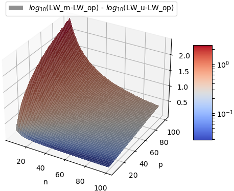
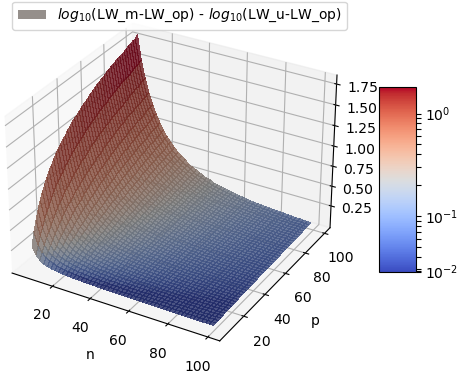
Figure 1: With $p$ the dimension, $n$ the number of samples, the axis $z$ shows the difference of the $log_{10}$ of the expected losses between LW_m and LW_u. The losses are relative to the theoretical bound LW_op. The samples are drawn with a Gaussian (left)/$t_{8.5}$ (right) distribution, $\Sigma=I_{p}$.

Convergence study

We now fix $c=p_{n}/n$ and study the convergence of the different algorithms we cited in the experimental setup. We only show the results with $c=1$ as the other cases only widen the differences but do not change the order. The cases $t_{10}$ and $t_{8.5}$-distributions are very similar, that’s why we show only the $t_{8.5}$ one. The key difference between the Gaussian case and the t-distribution, is that the OAS doesn’t converge in the latter, while not being so efficient in the Gaussian case which is tailored for it. The results are shown in figure 2.

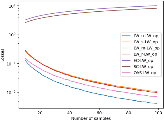
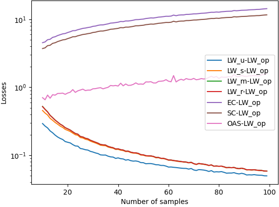
Figure 2: oss comparison to LW_op, Gaussian (left)/$t_{8.5}$ (right) distribution, $\Sigma=I_{p}$, $c=1$. Here, note that LW_ex and LW_op have both null loss, we didn’t plot them.

4.3.2 Covariance drawn from normalized Wishart

Study on a grid over (p,n)

The three estimators LW_r and LW_m have a very similar behavior compared to LW_u in this scenario, that’s why we will only show the comparison with LW_m, having the best performance among the two. Moreover, the results between the $t_{10}$ and $t_{8.5}$-distributions are very similar, so we will only show the $t_{8.5}$ case. The results are shown in figures 4 and 4. The black contour on the surface plots is the iso-line at level $0$, here it is where the losses are equal. In the case $p>n$, LW_u is far better than the other estimators, where the mean estimation affects a lot the overall covariance estimation. In a finite subset of the part $n>p$, LW_s is slightly better. LW_m presents no significant advantage compared to the two others.

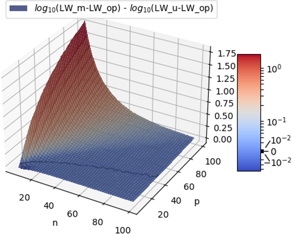
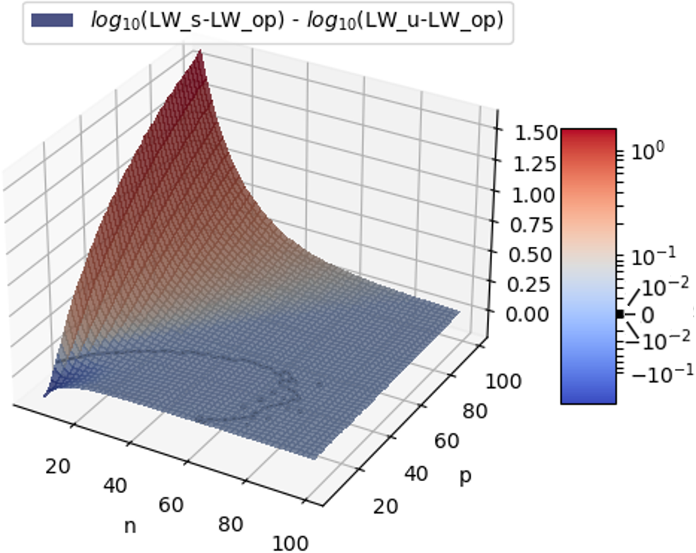
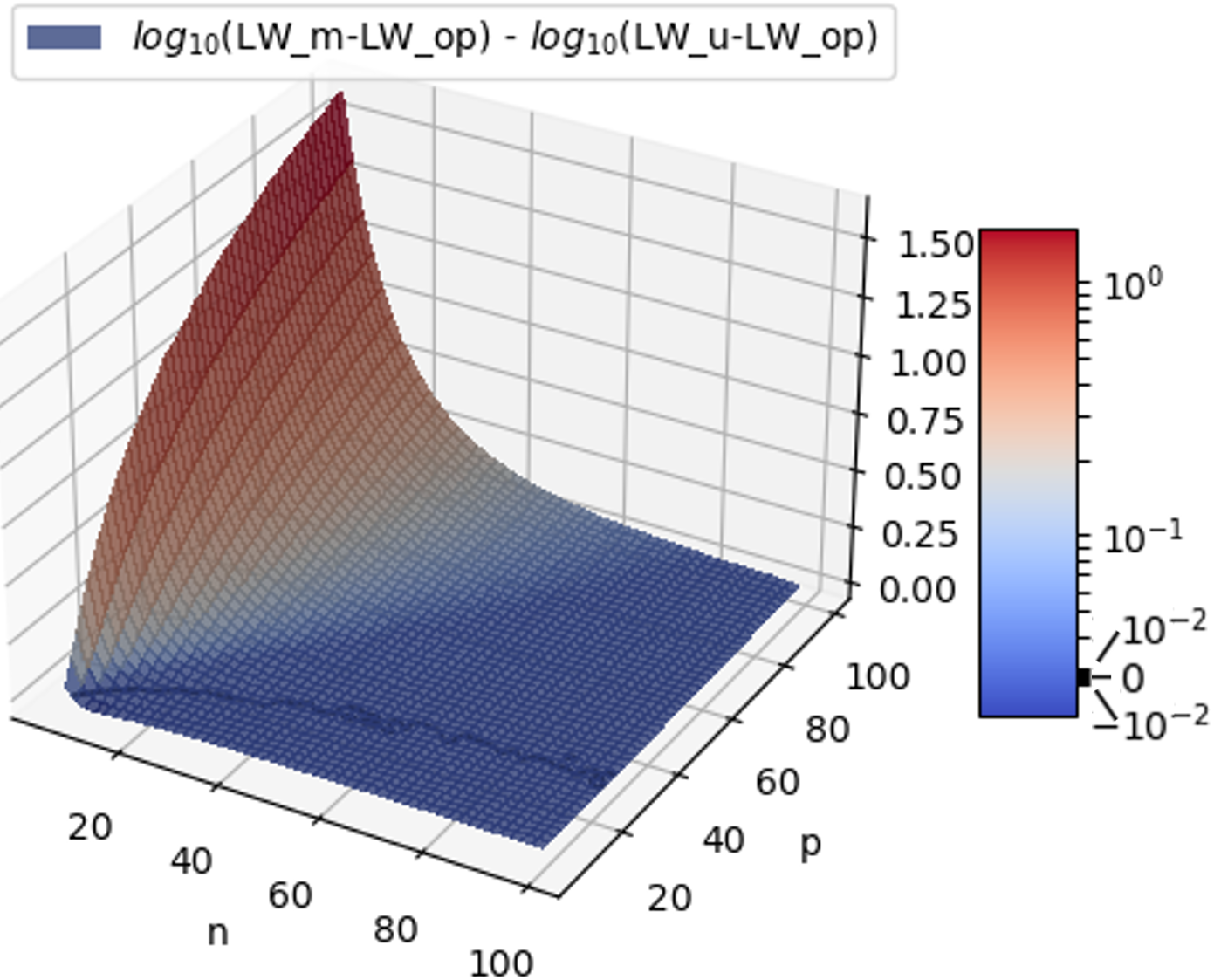
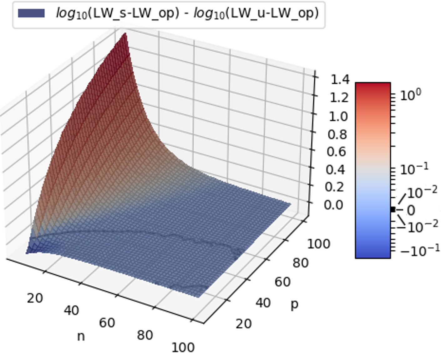
Figure 3: With $p$ the dimension, $n$ the number of samples, the axis $z$ shows the difference of the $log_{10}$ of the expected losses between LW_m (left)/LW_s (right) and LW_u. The losses are relative to the theoretical bound LW_op. Samples are drawn from a Gaussian distribution, random $\Sigma$. The black contour is the iso-line at level $0$, where the expected losses are equal.

Figure 4: With $p$ the dimension, $n$ the number of samples, the axis $z$ shows the difference of the $log_{10}$ of the expected losses between LW_m (left)/LW_s (right) and LW_u. The losses are relative to the theoretical bound LW_op. Samples are drawn from a $t_{8.5}$-distribution, random $\Sigma$. The black contour is the iso-line at level $0$, where the expected losses are equal.

Convergence study

We fix $c=p_{n}/n$ and study the convergence of the different algorithms we cited in the experimental setup. The cases $t_{10}$ and $t_{8.5}$-distributions being very similar, we only show $t_{8.5}$. The key difference between the Gaussian case and the t-distribution, is that the OAS doesn’t converge in the latter, while not being so efficient in the Gaussian case which is tailored for it. The results are shown in figures 6 and 6.

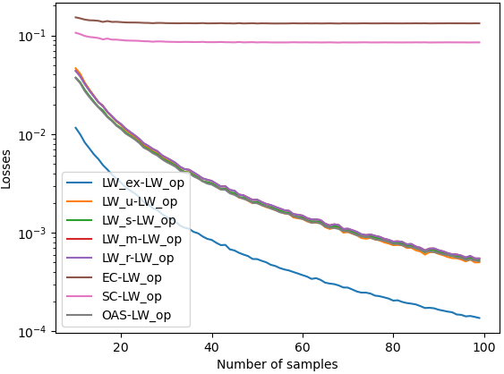
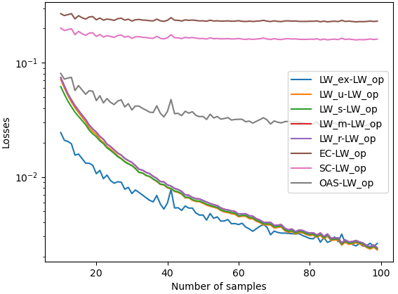
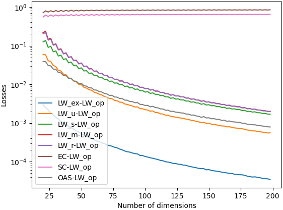
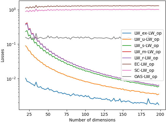
Figure 5: Loss comparison to LW_op, Gaussian (left)/$t_{8.5}$ (right) distribution, random $\Sigma$, $c=1$

Figure 6: Loss comparison to LW_op, Gaussian (left)/$t_{8.5}$ (right) distribution, random $\Sigma$, $c=4$. Note that LW_r and LW_m are not discernable.

5 Conclusion

In this work, we extended the linear shrinkage approach of Ledoit and Wolf [10] for covariance matrix estimation to the case where the mean of the distribution is unknown. Theoretically, we showed that in this case we have similar asymptotic properties as in the situation when the mean is known. Four different estimators emerged, three around those implemented in ScikitLearn or recommended by Ledoit and Wolf, and one naturally emerging from the theoretical proofs. Experimentally, the latter showed improved performances in a large spectrum of situations compared to ScikitLearn 1.2.2 baselines and to the three other estimators presented in the theoretical part. The gain in performance is particularly high when the dimension is bigger than the number of samples, while the differences are comparably low when dimension is smaller than the number of samples.

Ledoit and Wolf developed several non-linear shrinkage estimators where the mean is known [15, 16, 17]. Work needs to be conducted to investigate if similar approach can be used to extend their non-linear frameworks.

Funding

This research did not receive any specific grant from funding agencies in the public, commercial, or not-for-profit sectors.

6 Appendix A: Proofs of the technical results

For brevity, we omit the subscript $n$; but it is understood that everything depends on $n$. Coefficients of $\Lambda$ are denoted $\lambda_{ij}$, and if not stated otherwise, sum indices $i,j,l,m$ are in $\llbracket 1,p\rrbracket$ and $k_{1},k_{1}^{\prime},k_{2},k_{2}^{\prime},...$ are in $\llbracket 1,n\rrbracket$. Moreover, we denote $\bar{y}=\frac{1}{n}\sum_{k}y_{\cdot,k}$. We recall that, from Remark 2, as all the estimators are invariant by change of mean from the definition of $\tilde{X}=X-\sum_{k}X_{\cdot,k}$, we assume $\mathbb{E}[X]=0$ for the simplicity of notations.

6.1 Technical lemma

Frequently used identities are proven in preamble of the other proofs here.

6.1.1 Identity 1

Let $(i,j)\in\llbracket 1,p\rrbracket^{2}$, then:

$$\sum_{k}(y_{ik}-\bar{y}_{i})(y_{jk}-\bar{y}_{j}) =\sum_{k}\left(y_{ik}-\frac{1}{n}\sum_{k^{\prime}}y_{ik^{\prime}}\right)\left(y_{jk}-\frac{1}{n}\sum_{k^{\prime\prime}}y_{jk^{\prime\prime}}\right)$$ (4)

$$=\frac{1}{n^{2}}\sum_{k,k^{\prime},k^{\prime\prime}}(y_{ik}-y_{ik^{\prime}})(y_{jk}-y_{jk^{\prime\prime}})$$

$$=\frac{1}{n^{2}}\sum_{k,k^{\prime},k^{\prime\prime}}(y_{ik}y_{jk}-y_{ik^{\prime}}y_{jk}-y_{ik}y_{jk^{\prime\prime}}+y_{ik^{\prime}}y_{jk^{\prime\prime}})$$

$$=\frac{1}{n^{2}}\sum_{k,k^{\prime},k^{\prime\prime}}(y_{ik}y_{jk}-y_{ik}y_{jk^{\prime}}-y_{ik}y_{jk^{\prime}}+y_{ik}y_{jk^{\prime}})$$ (re-indexing)

$$=\frac{1}{n^{2}}\sum_{k,k^{\prime},k^{\prime\prime}}y_{ik}(y_{jk}-y_{jk^{\prime}})$$

$$\sum_{k}(y_{ik}-\bar{y}_{i})(y_{jk}-\bar{y}_{j}) =\frac{1}{n}\sum_{k,k^{\prime}\neq k}y_{ik}(y_{jk}-y_{jk^{\prime}}).$$

6.1.2 Identity 2

$$\frac{1}{p}\sum_{i,j}\lambda_{ij}^{2}=\lVert\Lambda\rVert_{p}^{2}=\lVert\Sigma\rVert_{p}^{2}=\lVert\Sigma-\mu I\rVert_{p}^{2}+\lVert\mu I\rVert_{p}^{2}=\alpha^{2}+\mu^{2}.$$ (5)

6.1.3 Identity 3

$$\frac{1}{p}\sum_{i,j}\lambda_{ii}\lambda_{jj}=\frac{1}{p}\left(\sum_{i}\lambda_{ii}\right)^{2}=\frac{1}{p}\tr(\Lambda)^{2}=\frac{1}{p}\tr(\Sigma)^{2}=p\langle\Sigma,I\rangle_{p}^{2}=p\mu^{2}.$$ (6)

6.2 Proof of Lemma 1

We have:

$$\lVert\Sigma\rVert^{2}=\lVert\Lambda\rVert^{2}=\frac{1}{p}\sum_{i=1}^{p}\mathbb{E}[y_{i1}^{2}]^{2}\leq\frac{1}{p}\sum_{i=1}^{p}\mathbb{E}[y_{i1}^{4}]\leq\sqrt{\frac{1}{p}\sum_{i=1}^{p}\mathbb{E}[y_{i1}^{8}]}\leq\sqrt{K_{2}}.$$ (7)

As $\mu=\langle\Sigma,I\rangle\leq\lVert\Sigma\rVert$, $\mu$ remains bounded as $n$ goes to infinity.
Also, $\alpha^{2}=\lVert\Sigma-\mu I\rVert^{2}=\lVert\Sigma\rVert^{2}-\mu^{2}$, so remains bounded as $n$ goes to infinity too.
For $\beta^{2}$, we will deeply decompose the expectation. This is not absolutely necessary to prove the boundedness, but the decomposition will be of utter importance in the following proofs. So, we have:

$$\beta^{2} =\mathbb{E}[\lVert S-\Sigma\rVert^{2}]$$ (8)

$$=\frac{1}{p}\sum_{i,j}\mathbb{E}\left[\left(\frac{1}{n-1}\sum_{k}(y_{ik}-\bar{y}_{i})(y_{jk}-\bar{y}_{j})-\lambda_{ij}\right)^{2}\right]$$

$$=\frac{1}{p}\sum_{i,j}\mathbb{E}\left[\left(\frac{1}{n(n-1)}\sum_{k,k^{\prime}\neq k}y_{ik}(y_{jk}-y_{jk^{\prime}})-\lambda_{ij}\right)^{2}\right]\text{ (Identity 1)}$$

$$\beta^{2} =\frac{1}{p}\sum_{i,j}\frac{1}{n^{2}(n-1)^{2}}\sum_{k_{1}}\sum_{k_{1}^{\prime}\neq k_{1}}\sum_{k_{2}}\sum_{k_{2}^{\prime}\neq k_{2}}\mathbb{E}\left[\left(y_{ik_{1}}(y_{jk_{1}}-y_{jk_{1}^{\prime}})-\lambda_{ij}\right)\left(y_{ik_{2}}(y_{jk_{2}}-y_{jk_{2}^{\prime}})-\lambda_{ij}\right)\right].$$

We denote, for $k_{1},k_{1}^{\prime}\neq k_{1},k_{2},k_{2}^{\prime}\neq k_{2}$:

$$E_{ij}(k_{1},k_{1}^{\prime},k_{2},k_{2}^{\prime})=\mathbb{E}\left[\left(y_{ik_{1}}(y_{jk_{1}}-y_{jk_{1}^{\prime}})-\lambda_{ij}\right)\left(y_{ik_{2}}(y_{jk_{2}}-y_{jk_{2}^{\prime}})-\lambda_{ij}\right)\right].$$ (9)

• If $|\{k_{1},k_{1}^{\prime}\}\cap\{k_{2},k_{2}^{\prime}\}|=0$: $E_{ij}(k_{1},k_{1}^{\prime},k_{2},k_{2}^{\prime})=0$.

• If $|\{k_{1},k_{1}^{\prime}\}\cap\{k_{2},k_{2}^{\prime}\}|=1$:

  • If $k_{1}=k_{2}$: then $k_{1}^{\prime}\neq k_{2}^{\prime}$, and $k_{1}\neq k_{2}^{\prime}$. So,

    $$E_{ij}(k_{1},k_{1}^{\prime},k_{1},k_{2}^{\prime}) =\mathbb{E}\left[\left(y_{ik_{1}}(y_{jk_{1}}-y_{jk_{1}^{\prime}})-\lambda_{ij}\right)\left(y_{ik_{1}}(y_{jk_{1}}-y_{jk_{2}^{\prime}})-\lambda_{ij}\right)\right]$$ (10)

    $$=\mathbb{E}\left[\left(y_{ik_{1}}y_{jk_{1}}-\lambda_{ij}\right)^{2}\right]$$

    $$=\mathbb{V}[y_{ik_{1}}y_{jk_{1}}]$$

    $$E_{ij}(k_{1},k_{1}^{\prime},k_{1},k_{2}^{\prime}) =\mathbb{V}[y_{i1}y_{j1}].$$

    Moreover, the number of terms in the initial sum on $k_{1},k_{1}^{\prime}\neq k_{1},k_{2},k_{2}^{\prime}\neq k_{2}$ satisfying the conditions of this case on the indices is:

    $$\left|\left\{(k_{1},k_{1}^{\prime},k_{2},k_{2}^{\prime})\in\llbracket 1,n\rrbracket^{4}|k_{1}^{\prime}\neq k_{1},k_{2}^{\prime}\neq k_{2},|\{k_{1},k_{1}^{\prime}\}\cap\{k_{2},k_{2}^{\prime}\}|=1,k_{1}=k_{2}\right\}\right|$$ (11)

    $$=n(n-1)(n-2).$$

  • If $k_{1}=k_{2}^{\prime}$ (or similarly $k_{1}^{\prime}=k_{2}$): then $k_{1}^{\prime}\neq k_{2}$ and $k_{1}\neq k_{2}$. So, $E_{ij}(k_{1},k_{1}^{\prime},k_{2},k_{1})=0$.

  • If $k_{1}^{\prime}=k_{2}^{\prime}$: $E_{ij}(k_{1},k_{1}^{\prime},k_{2},k_{1}^{\prime})=0$.

• If $|\{k_{1},k_{1}^{\prime}\}\cap\{k_{2},k_{2}^{\prime}\}|=2$:

  • If $k_{1}=k_{2}$ and $k_{1}^{\prime}=k_{2}^{\prime}$: then $k_{1}\neq k_{1}^{\prime}$. So,

    $$E_{ij}(k_{1},k_{1}^{\prime},k_{1},k_{1}^{\prime}) =\mathbb{E}\left[\left(y_{ik_{1}}(y_{jk_{1}}-y_{jk_{1}^{\prime}})-\lambda_{ij}\right)^{2}\right]$$ (12)

    $$=\mathbb{V}[y_{ik_{1}}y_{jk_{1}}]+\lambda_{ii}\lambda_{jj}$$

    $$E_{ij}(k_{1},k_{1}^{\prime},k_{1},k_{1}^{\prime}) =\mathbb{V}[y_{i1}y_{j1}]+\lambda_{ii}\lambda_{jj}.$$

    Moreover, the number of terms in the initial sum on $k_{1},k_{1}^{\prime}\neq k_{1},k_{2},k_{2}^{\prime}\neq k_{2}$ satisfying the conditions of this case on the indices is:

    $$\left|\left\{(k_{1},k_{1}^{\prime},k_{2},k_{2}^{\prime})\in\llbracket 1,n\rrbracket^{4}|k_{1}^{\prime}\neq k_{1},k_{2}^{\prime}\neq k_{2},|\{k_{1},k_{1}^{\prime}\}\cap\{k_{2},k_{2}^{\prime}\}|=2,k_{1}=k_{2},k_{1}^{\prime}=k_{2}^{\prime}\right\}\right|$$ (13)

    $$=n(n-1).$$

  • If $k_{1}=k_{2}^{\prime}$ and $k_{1}^{\prime}=k_{2}$: then $k_{1}\neq k_{1}^{\prime}$. So,

    $$E_{ij}(k_{1},k_{1}^{\prime},k_{1}^{\prime},k_{1}) =\mathbb{E}\left[\left(y_{ik_{1}}(y_{jk_{1}}-y_{jk_{1}^{\prime}})-\lambda_{ij}\right)\left(y_{ik_{1}^{\prime}}(y_{jk_{1}^{\prime}}-y_{jk_{1}})-\lambda_{ij}\right)\right]$$ (14)

    $$E_{ij}(k_{1},k_{1}^{\prime},k_{1}^{\prime},k_{1}) =\lambda_{ij}^{2}.$$

    Moreover, the number of terms in the initial sum on $k_{1},k_{1}^{\prime}\neq k_{1},k_{2},k_{2}^{\prime}\neq k_{2}$ satisfying the conditions of this case on the indices is:

    $$\left|\left\{(k_{1},k_{1}^{\prime},k_{2},k_{2}^{\prime})\in\llbracket 1,n\rrbracket^{4}|k_{1}^{\prime}\neq k_{1},k_{2}^{\prime}\neq k_{2},|\{k_{1},k_{1}^{\prime}\}\cap\{k_{2},k_{2}^{\prime}\}|=2,k_{1}=k_{2}^{\prime},k_{1}^{\prime}=k_{2}\right\}\right|$$ (15)

    $$=n(n-1).$$

Using the latter decomposition on $(k_{1},k_{1}^{\prime},k_{2},k_{2}^{\prime})$, we deduce:

$$\beta^{2} =\frac{1}{p}\sum_{i,j}\frac{1}{n^{2}(n-1)^{2}}\left[n(n-1)(n-2)\mathbb{V}[y_{i1}y_{j1}]+n(n-1)(\mathbb{V}[y_{i1}y_{j1}]+\lambda_{ii}\lambda_{jj})+n(n-1)\lambda_{ij}^{2}\right]$$ (16)

$$\beta^{2} =\frac{1}{pn}\sum_{i,j}\mathbb{V}[y_{i1}y_{j1}]+\frac{p+1}{n(n-1)}\mu^{2}+\frac{1}{n(n-1)}\alpha^{2}\text{ (Identities 2 \& 3).}$$

• $\mu^{2}$ is bounded when $n$ goes to infinity, so $\frac{p+1}{n(n-1)}\mu^{2}\leq\frac{K_{1}+1}{n-1}\mu^{2}$ remains bounded too.
  

• $\alpha^{2}$ is bounded when $n$ goes to infinity, so $\frac{1}{n(n-1)}\alpha^{2}$ remains bounded too.
  

• Finally, following (Ledoit and Wolf, 2004) [10] proof of Lemma 3.1,

  $$\frac{1}{pn}\sum_{i,j}\mathbb{V}[y_{i1}y_{j1}] \leq\frac{1}{pn}\sum_{i,j}\mathbb{E}[y_{i1}^{2}y_{j1}^{2}]$$ (17)

  $$\leq\frac{1}{pn}\sum_{i,j}\sqrt{\mathbb{E}[y_{i1}^{4}]\mathbb{E}[y_{j1}^{4}]}$$ (Cauchy-Schwarz)

  $$\leq\frac{1}{pn}\sum_{i,j}\sqrt[4]{\mathbb{E}[y_{i1}^{8}]\mathbb{E}[y_{j1}^{8}]}$$ (Cauchy-Schwarz)

  $$=\frac{p}{n}\left(\sum_{i}\frac{1}{p}\sqrt[4]{\mathbb{E}[y_{i1}^{8}]}\right)^{2}$$

  $$\leq\frac{p}{n}\sqrt{\left(\sum_{i}\frac{1}{p}\mathbb{E}[y_{i1}^{8}]\right)} \text{(Jensen for }\sqrt[4]{\cdot}\text{ concave)}$$

  $$\frac{1}{pn}\sum_{i,j}\mathbb{V}[y_{i1}y_{j1}] \leq K_{1}\sqrt{K_{2}}.$$

So, $\beta^{2}$ remains bounded as $n$ goes to infinity. Finally, $\delta^{2}=\alpha^{2}+\beta^{2}$ is also bounded as $n$ goes to infinity, which conclude the proof of the lemma.

6.3 Proof of Theorem 1

We have:

$$\mu^{2}+\theta^{2} =\left(\mathbb{E}\left[\frac{1}{p}\sum_{i}y_{i1}^{2}\right]\right)^{2}+\mathbb{V}\left[\frac{1}{p}\sum_{i}y_{i1}^{2}\right]$$ (18)

$$=\mathbb{E}\left[\left(\frac{1}{p}\sum_{i}y_{i1}^{2}\right)^{2}\right]$$

$$=\frac{1}{p^{2}}\sum_{ij}\mathbb{E}\left[y_{i1}^{2}y_{j1}^{2}\right]$$

$$=\frac{1}{p^{2}}\sum_{ij}\mathbb{V}\left[y_{i1}y_{j1}\right]+\lambda_{ij}^{2}$$

$$=\frac{1}{p}(\alpha^{2}+\mu^{2})+\frac{1}{p^{2}}\sum_{ij}\mathbb{V}\left[y_{i1}y_{j1}\right]$$ (Identity 2)

$$\mu^{2}+\theta^{2} \leq\frac{1}{p}(\alpha^{2}+\mu^{2})+\sqrt{K_{2}}$$ (Proof of Lemma 1).

As $\alpha^{2}$ and $\mu^{2}$ remains bounded as $n$ goes to infinity, so is $\theta^{2}$. And, from the proof of Lemma 1:

$$\beta^{2}=\frac{1}{pn}\sum_{i,j}\mathbb{V}[y_{i1}y_{j1}]+\frac{p+1}{n(n-1)}\mu^{2}+\frac{1}{n(n-1)}\alpha^{2}.$$ (19)

So,

$$\beta^{2} =\frac{p}{n}\left(\mu^{2}+\theta^{2}-\frac{1}{p}(\alpha^{2}+\mu^{2})\right)+\frac{p+1}{n(n-1)}\mu^{2}+\frac{1}{n(n-1)}\alpha^{2}$$ (20)

$$=\frac{p}{n}\left(\mu^{2}+\theta^{2}\right)-\frac{1}{n(n-1)}\alpha^{2}+\frac{p-n+2}{n(n-1)}\mu^{2}.$$

As $\alpha^{2}$, $\mu^{2}$ and $\frac{p}{n}$ remains bounded as $n$ goes to infinity, immediately we have:

$$\beta^{2}-\frac{p}{n}\left(\mu^{2}+\theta^{2}\right)\underset{n\rightarrow\infty}{\longrightarrow}0.$$ (21)

6.4 Proof of Lemma 2

By linearity of the inner product, we trivially have: $\mathbb{E}[m]=\mu$. For the quartic mean convergence, we write:

$$\mathbb{E}[(m-\mu)^{4}] =\mathbb{E}\left[\left(\frac{1}{p}\sum_{i}\frac{1}{n-1}\sum_{k}\left((y_{ik}-\bar{y}_{i})^{2}-\frac{n-1}{n}\lambda_{ii}\right)\right)^{4}\right]$$ (22)

$$=\mathbb{E}\left[\left(\frac{1}{n-1}\sum_{k}\frac{1}{p}\sum_{i}\left((y_{ik}-\bar{y}_{i})^{2}-\frac{n-1}{n}\lambda_{ii}\right)\right)^{4}\right].$$

Using Identity 1, we obtain:

$$\mathbb{E}[(m-\mu)^{4}] =\frac{1}{(n-1)^{4}}\sum_{\begin{subarray}{c}k_{1},k_{2},k_{3},k_{4}\\ k_{1}^{\prime},k_{2}^{\prime},k_{3}^{\prime},k_{4}^{\prime}\end{subarray}} \mathbb{E}\left[\left[\frac{1}{p}\sum_{i}\frac{1}{n}\left(y_{ik_{1}}^{2}-\lambda_{ii}\right)-\frac{1}{n}\left(y_{ik_{1}}y_{ik_{1}^{\prime}}-\delta_{k_{1}=k_{1}^{\prime}}\lambda_{ii}\right)\right]\right.$$ (23)

$$\times\left[\frac{1}{p}\sum_{i}\frac{1}{n}\left(y_{ik_{2}}^{2}-\lambda_{ii}\right)-\frac{1}{n}\left(y_{ik_{2}}y_{ik_{2}^{\prime}}-\delta_{k_{2}=k_{2}^{\prime}}\lambda_{ii}\right)\right]$$

$$\times\left[\frac{1}{p}\sum_{i}\frac{1}{n}\left(y_{ik_{3}}^{2}-\lambda_{ii}\right)-\frac{1}{n}\left(y_{ik_{3}}y_{ik_{3}^{\prime}}-\delta_{k_{3}=k_{3}^{\prime}}\lambda_{ii}\right)\right]$$

$$\times\left.\left[\frac{1}{p}\sum_{i}\frac{1}{n}\left(y_{ik_{4}}^{2}-\lambda_{ii}\right)-\frac{1}{n}\left(y_{ik_{4}}y_{ik_{4}^{\prime}}-\delta_{k_{4}=k_{4}^{\prime}}\lambda_{ii}\right)\right]\right].$$

$$\mathbb{E}[(m-\mu)^{4}] = \frac{1}{(n-1)^{4}}\sum_{\begin{subarray}{c}k_{1},k_{2},k_{3},k_{4}\\ k_{1}^{\prime},k_{2}^{\prime},k_{3}^{\prime},k_{4}^{\prime}\end{subarray}}\mathbb{E}\left[\prod_{s=1}^{4}\left(\frac{1}{pn}\sum_{i}(y_{ik_{s}}^{2}-\lambda_{ii})\right)\right]$$ (24)

$$-4\mathbb{E}\left[\prod_{s=1}^{3}\left(\frac{1}{pn}\sum_{i}(y_{ik_{s}}^{2}-\lambda_{ii})\right)\left(\frac{1}{pn}\sum_{i}(y_{ik_{4}}y_{ik_{4}^{\prime}}-\delta_{k_{4}=k_{4}^{\prime}}\lambda_{ii})\right)\right]$$

$$+6\mathbb{E}\left[\prod_{s=1}^{2}\left(\frac{1}{pn}\sum_{i}(y_{ik_{s}}^{2}-\lambda_{ii})\right)\prod_{t=3}^{4}\left(\frac{1}{pn}\sum_{i}(y_{ik_{t}}y_{ik_{t}^{\prime}}-\delta_{k_{t}=k_{t}^{\prime}}\lambda_{ii})\right)\right]$$

$$-4\mathbb{E}\left[\left(\frac{1}{pn}\sum_{i}(y_{ik_{1}}^{2}-\lambda_{ii})\right)\prod_{t=2}^{4}\left(\frac{1}{pn}\sum_{i}(y_{ik_{t}}y_{ik_{t}^{\prime}}-\delta_{k_{t}=k_{t}^{\prime}}\lambda_{ii})\right)\right]$$

$$+\mathbb{E}\left[\prod_{t=1}^{4}\left(\frac{1}{pn}\sum_{i}(y_{ik_{t}}y_{ik_{t}^{\prime}}-\delta_{k_{t}=k_{t}^{\prime}}\lambda_{ii})\right)\right].$$

If $k_{1},k_{1}^{\prime},k_{2},k_{2}^{\prime},k_{3},k_{3}^{\prime},k_{4},k_{4}^{\prime}$ are all different, then the expectation in the sum equals $0$. So there are at most $28n^{7}+O(n^{6})$ non-zero terms in the sum.
Now, let’s find a bound of those expectations. Let’s first note that, for all $(k,k^{\prime})\in\llbracket 1,n\rrbracket^{2}$ and $i\in\llbracket 1,p\rrbracket$:

$$\mathbb{E}\left[\left(y_{ik}y_{ik^{\prime}}-\delta_{k_{t}=k_{t}^{\prime}}\lambda_{ii}\right)^{4}\right]=\mathbb{E}\left[\left(y_{ik}y_{ik^{\prime}}-\mathbb{E}[y_{ik}y_{ik^{\prime}}]\right)^{4}\right]=$$ (25)

$$\mathbb{E}[(y_{ik}y_{ik^{\prime}})^{4}]-4\mathbb{E}[(y_{ik}y_{ik^{\prime}})^{3}]\mathbb{E}[y_{ik}y_{ik^{\prime}}]+6\mathbb{E}[(y_{ik}y_{ik^{\prime}})^{2}]\mathbb{E}[y_{ik}y_{ik^{\prime}}]^{2}-3\mathbb{E}[y_{ik}y_{ik^{\prime}}]^{4}.$$

If $k=k^{\prime}$ then $\mathbb{E}[(y_{ik}y_{ik^{\prime}})^{3}]\mathbb{E}[y_{ik}y_{ik^{\prime}}]\geq 0$ and if $k\neq k^{\prime}$, $\mathbb{E}[(y_{ik}y_{ik^{\prime}})^{3}]\mathbb{E}[y_{ik}y_{ik^{\prime}}]=0\geq 0$, so:

$$\mathbb{E}\left[\left(y_{ik}y_{ik^{\prime}}-\delta_{k_{t}=k_{t}^{\prime}}\lambda_{ii}\right)^{4}\right] \leq\mathbb{E}[(y_{ik}y_{ik^{\prime}})^{4}]+6\mathbb{E}[(y_{ik}y_{ik^{\prime}})^{2}]E[y_{ik}y_{ik^{\prime}}]^{2}$$ (26)

$$\leq\mathbb{E}[(y_{ik}y_{ik^{\prime}})^{4}]+6\mathbb{E}[(y_{ik}y_{ik^{\prime}})^{4}]$$ (Cauchy-Schwarz)

$$\mathbb{E}\left[\left(y_{ik}y_{ik^{\prime}}-\delta_{k_{t}=k_{t}^{\prime}}\lambda_{ii}\right)^{4}\right] \leq 7\mathbb{E}[(y_{ik}y_{ik^{\prime}})^{4}].$$

Back to the bound of our expectation, let $N\in\llbracket 1,4\rrbracket$, and we have:

$$\left|\mathbb{E}\left[\prod_{s=1}^{N}\left(\frac{1}{pn}\sum_{i}(y_{ik_{s}}^{2}-\lambda_{ii})\right)\prod_{t=N+1}^{4}\left(\frac{1}{pn}\sum_{i}(y_{ik_{t}}y_{ik_{t}^{\prime}}-\delta_{k_{t}=k_{t}^{\prime}}\lambda_{ii})\right)\right]\right|$$ (27)

$$\leq\frac{1}{n^{4}}\prod_{s=1}^{N}\sqrt[4]{\mathbb{E}\left[\left(\frac{1}{p}\sum_{i}(y_{ik_{s}}^{2}-\lambda_{ii})\right)^{4}\right]}\prod_{t=N+1}^{4}\sqrt[4]{\mathbb{E}\left[\left(\frac{1}{p}\sum_{i}(y_{ik_{t}}y_{ik_{t}^{\prime}}-\delta_{k_{t}=k_{t}^{\prime}}\lambda_{ii})\right)^{4}\right]}$$ (2 Cauchy-Schwarz)

$$\leq\frac{1}{n^{4}}\prod_{s=1}^{N}\sqrt[4]{\frac{1}{p}\sum_{i}\mathbb{E}[(y_{ik_{s}}^{2}-\lambda_{ii})^{4}]}\prod_{t=N+1}^{4}\sqrt[4]{\frac{1}{p}\sum_{i}\mathbb{E}[(y_{ik_{t}}y_{ik_{t}^{\prime}}-\delta_{k_{t}=k_{t}^{\prime}})^{4}]}$$ (Jensen)

$$\leq\frac{7}{n^{4}}\prod_{s=1}^{N}\sqrt[4]{\frac{1}{p}\sum_{i}\mathbb{E}[y_{ik_{s}}^{8}]}\prod_{t=N+1}^{4}\sqrt[4]{\frac{1}{p}\sum_{i}\mathbb{E}[y_{ik_{t}}^{4}y_{ik_{t}^{\prime}}^{4}]}$$ (Previous remark)

$$\leq\frac{7}{n^{4}}\prod_{s=1}^{N}\sqrt[4]{\frac{1}{p}\sum_{i}\mathbb{E}[y_{ik_{s}}^{8}]}\prod_{t=N+1}^{4}\sqrt[4]{\frac{1}{p}\sum_{i}\mathbb{E}[y_{ik_{t}}^{8}]} \text{(Jensen if }k_{t}\neq k_{t}^{\prime}\text{)}$$

$$\leq\frac{7}{n^{4}}\prod_{s=1}^{4}\sqrt[4]{\frac{1}{p}\sum_{i}\mathbb{E}[y_{ik_{s}}^{8}]}$$

$$\leq\frac{7}{n^{4}}\frac{1}{p}\sum_{i}\mathbb{E}[y_{ik_{1}}^{8}]$$

$$\leq\frac{7K_{2}}{n^{4}}.$$

So, in conclusion of this proof,

$$\mathbb{E}[(m-\mu)^{4}]\leq 7(1+4+6+4+1)\frac{28n^{7}+O(n^{6})}{n^{4}(n-1)^{4}}K_{2}\underset{n\rightarrow\infty}{\longrightarrow}0.$$ (28)

6.5 Proof of Corollary 2

We have:

$$\mathbb{V}[m^{2}] =\mathbb{E}[m^{4}]-\mathbb{E}[m^{2}]^{2}$$ (29)

$$=\mathbb{E}[(m-\mu+\mu)^{4}]-\mathbb{E}[(m-\mu+\mu)^{2}]^{2}$$

$$=\mathbb{E}[(m-\mu)^{4}]+4\mathbb{E}[(m-\mu)^{3}]\mu+6\mathbb{E}[(m-\mu)^{2}]\mu^{2}+\mu^{4}-\mathbb{E}[(m-\mu)^{2}]^{2}-2\mathbb{E}[(m-\mu)^{2}]\mu^{2}-\mu^{4}$$

$$\mathbb{V}[m^{2}] =\mathbb{E}[(m-\mu)^{4}]+4\mathbb{E}[(m-\mu)^{3}]\mu+4\mathbb{E}[(m-\mu)^{2}]\mu^{2}-\mathbb{E}[(m-\mu)^{2}]^{2}.$$

And, from Lemma 2, $\mathbb{E}[(m-\mu)^{4}]{\rightarrow}0$, and so goes for the smaller moments by Jensen inequality, and $\mu$ is bounded from Lemma 1. So, $\mathbb{V}[m^{2}]{\rightarrow}0$.

6.6 Proof of Lemma 3

6.6.1 Preliminary combinatorial result

Let $K\in\mathbb{N}^{*}$, and $K$ indices $(k_{1},...,k_{K})\in\llbracket 1,n\rrbracket^{K}$.
Let’s associate a graph with $K$ vertices $\mathcal{V}=\{1,...,K\}$ to this set of indices. The set of edges $\mathcal{E}$ is built as following: there is an edge between the node $a\in\mathcal{V}$ and $b\in\mathcal{V}$, $a\neq b$ (we don’t allow self-loops), if the corresponding indices are equal, i.e if $k_{a}=k_{b}$. We finally define our graph $\mathcal{G}=(\mathcal{V},\mathcal{E})$.

Proposition 1.

Let $\mathcal{G}=(\mathcal{V},\mathcal{E})$ a graph with $K$ vertices generated from some indices $(k_{1}^{(0)},...,k_{K}^{(0)})\in\llbracket 1,n\rrbracket^{K}$ with the procedure described previously. Suppose $\mathcal{G}$ has $C\in\llbracket 1,K\rrbracket$ connected components. Then, there are $\prod_{i=0}^{C-1}(n-i)$ set of indices $(k_{1},...,k_{K})\in\llbracket 1,n\rrbracket^{K}$ which have the associated graph $\mathcal{G}$.

For each node $v\in\mathcal{V}$, $v$ belongs to a unique connected component that we denote $c(v)\in\llbracket 1,C\rrbracket$. Then, the function:

$$x\in\left\{x\in\llbracket 1,n\rrbracket^{C},x_{1},...,x_{C}\text{ all different}\right\}\mapsto(x_{c(1)},....,x_{c(K)})$$

is a bijection between $\left\{x\in\llbracket 1,n\rrbracket^{C},x_{1},...,x_{C}\text{ all different}\right\}$ and
$\left\{(k_{1},...,k_{K})\in\llbracket 1,n\rrbracket^{K}\text{ which have the associated graph }\mathcal{G}\right\}$. Immediately, we deduce that its cardinal is equal to $\prod_{i=0}^{C-1}(n-i)$.

6.6.2 Proof of Lemma 3

From the proof of Lemma 3.3 in (Ledoit and Wolf, 2004) [10], we have:

$$d^{2}-\delta^{2}=-(m-\mu)^{2}+2\mu(\mu-m)+\left(\lVert S\rVert^{2}-\mathbb{E}[\lVert S\rVert^{2}]\right).$$ (30)

The first two terms converge to $0$ in quadratic mean thanks to Lemma 2. Let’s show that the last term converges to $0$ in quadratic mean too, i.e $\mathbb{V}[\lVert S\rVert^{2}]\underset{n\rightarrow\infty}{\longrightarrow}0$ .
Decomposing $\lVert S\rVert^{2}$, we have:

$$\lVert S\rVert^{2} = \frac{1}{p}\left\lVert\frac{1}{n-1}\sum_{k}\left(X_{\cdot k}-\bar{X}\right)\left(X_{\cdot k}-\bar{X}\right)^{T}\right\rVert^{2}$$ (31)

$$= \frac{1}{p}\left\lVert\frac{1}{n-1}\sum_{k}\left(Y_{\cdot k}-\bar{Y}\right)\left(Y_{\cdot k}-\bar{Y}\right)^{T}\right\rVert^{2}$$

$$= \frac{1}{p(n-1)^{2}}\sum_{i,j}\left(\sum_{k}(y_{ik}-\bar{y}_{i})(y_{jk}-\bar{y}_{j})\right)^{2}$$

$$= \frac{1}{p(n-1)^{2}}\sum_{i,j}\left(\frac{1}{n}\sum_{k,k^{\prime}}y_{ik}(y_{jk}-y_{jk^{\prime}})\right)^{2}\text{ (Identity 1)}$$

$$= \frac{1}{pn^{2}(n-1)^{2}}\sum_{i,j}\left(\sum_{k_{1},k_{1}^{\prime}\neq k_{1}}y_{ik_{1}}(y_{jk_{1}}-y_{jk_{1}^{\prime}})\right)\left(\sum_{k_{2},k_{2}^{\prime}\neq k_{2}}y_{ik_{2}}(y_{jk_{2}}-y_{jk_{2}^{\prime}})\right)$$

$$= \frac{p}{n^{2}(n-1)^{2}}\sum_{k_{1},k_{1}^{\prime}\neq k_{1}}\sum_{k_{2}=k_{1}^{\prime},k_{2}^{\prime}\neq k_{2}}\frac{1}{p^{2}}\sum_{i,j}y_{ik_{1}}y_{ik_{2}}\left(y_{jk_{1}}y_{jk_{2}}-y_{jk_{1}}y_{jk_{2}^{\prime}}-y_{jk_{1}^{\prime}}y_{jk_{2}}+y_{jk_{1}^{\prime}}y_{jk_{2}^{\prime}}\right)$$

$$+\frac{p}{n^{2}(n-1)^{2}}\sum_{k_{1},k_{1}^{\prime}\neq k_{1}}\sum_{k_{2}\neq k_{1}^{\prime},k_{2}^{\prime}\neq k_{2}}\frac{1}{p^{2}}\sum_{i,j}y_{ik_{1}}y_{ik_{2}}\left(y_{jk_{1}}y_{jk_{2}}-y_{jk_{1}}y_{jk_{2}^{\prime}}-y_{jk_{1}^{\prime}}y_{jk_{2}}+y_{jk_{1}^{\prime}}y_{jk_{2}^{\prime}}\right)$$

$$= \frac{p}{n^{2}(n-1)^{2}}\sum_{k_{1},k_{1}^{\prime}\neq k_{1}}\sum_{k_{2}=k_{1}^{\prime},k_{2}^{\prime}\neq k_{2}}\frac{1}{p^{2}}\sum_{i,j}y_{ik_{1}}y_{ik_{1}^{\prime}}\left(y_{jk_{1}}y_{jk_{1}^{\prime}}-y_{jk_{1}}y_{jk_{2}^{\prime}}-y_{jk_{1}^{\prime}}^{2}+y_{jk_{1}^{\prime}}y_{jk_{2}^{\prime}}\right)$$

$$+\frac{p}{n^{2}(n-1)^{2}}\sum_{k_{1},k_{1}^{\prime}\neq k_{1}}\sum_{k_{2}\neq k_{1}^{\prime},k_{2}^{\prime}\neq k_{2}}\frac{1}{p^{2}}\sum_{i,j}y_{ik_{1}}y_{ik_{2}}\left(y_{jk_{1}}y_{jk_{2}}-y_{jk_{1}}y_{jk_{2}^{\prime}}-y_{jk_{1}^{\prime}}y_{jk_{2}}+y_{jk_{1}^{\prime}}y_{jk_{2}^{\prime}}\right)$$

$$= \frac{p}{n^{2}(n-1)^{2}}\sum_{k_{1},k_{1}^{\prime}\neq k_{1},k_{2}^{\prime}\neq k_{1}^{\prime}}\left(\left(\frac{1}{p}\sum_{i}y_{ik_{1}}y_{ik_{1}^{\prime}}\right)^{2}-\frac{1}{p^{2}}\sum_{i,j}y_{ik_{1}}y_{ik_{1}^{\prime}}\left(y_{jk_{1}}y_{jk_{2}^{\prime}}+y_{jk_{1}^{\prime}}^{2}-y_{jk_{1}^{\prime}}y_{jk_{2}^{\prime}}\right)\right)$$

$$+\frac{p}{n^{2}(n-1)^{2}}\sum_{\begin{subarray}{c}k_{1},k_{1}^{\prime}\neq k_{1}\\ k_{2}\neq k_{1}^{\prime},k_{2}^{\prime}\neq k_{2}\end{subarray}}\left(\left(\frac{1}{p}\sum_{i}y_{ik_{1}}y_{ik_{2}}\right)^{2}-\frac{1}{p^{2}}\sum_{i,j}y_{ik_{1}}y_{ik_{2}}\left(y_{jk_{1}}y_{jk_{2}^{\prime}}+y_{jk_{1}^{\prime}}y_{jk_{2}}-y_{jk_{1}^{\prime}}y_{jk_{2}^{\prime}}\right)\right).$$

$$\lVert S\rVert^{2} =\frac{p}{n^{2}(n-1)}\sum_{k_{1},k_{1}^{\prime}\neq k_{1}}\left(\frac{1}{p}\sum_{i}y_{ik_{1}}y_{ik_{1}^{\prime}}\right)^{2} (t1)$$ (32)

$$-\frac{p}{n^{2}(n-1)^{2}}\sum_{k_{1},k_{1}^{\prime}\neq k_{1},k_{2}^{\prime}\neq k_{1}^{\prime}}\frac{1}{p^{2}}\sum_{i,j}y_{ik_{1}}y_{ik_{1}^{\prime}}y_{jk_{1}}y_{jk_{2}^{\prime}} (t2)$$

$$-\frac{p}{n^{2}(n-1)}\sum_{k_{1},k_{1}^{\prime}\neq k_{1}}\frac{1}{p^{2}}\sum_{i,j}y_{ik_{1}}y_{ik_{1}^{\prime}}y_{jk_{1}^{\prime}}^{2} (t3)$$

$$+\frac{p}{n^{2}(n-1)^{2}}\sum_{k_{1},k_{1}^{\prime}\neq k_{1},k_{2}^{\prime}\neq k_{1}^{\prime}}\frac{1}{p^{2}}\sum_{i,j}y_{ik_{1}}y_{ik_{1}^{\prime}}y_{jk_{1}^{\prime}}y_{jk_{2}^{\prime}} (t4)$$

$$+\frac{p}{n^{2}(n-1)^{2}}\sum_{\begin{subarray}{c}k_{1},k_{1}^{\prime}\neq k_{1}\\ k_{2}\neq k_{1}^{\prime},k_{2}^{\prime}\neq k_{2}\end{subarray}}\left(\frac{1}{p}\sum_{i}y_{ik_{1}}y_{ik_{2}}\right)^{2} (t5)$$

$$-\frac{p}{n^{2}(n-1)^{2}}\sum_{\begin{subarray}{c}k_{1},k_{1}^{\prime}\neq k_{1}\\ k_{2}\neq k_{1}^{\prime},k_{2}^{\prime}\neq k_{2}\end{subarray}}\frac{1}{p^{2}}\sum_{i,j}y_{ik_{1}}y_{ik_{2}}y_{jk_{1}}y_{jk_{2}^{\prime}} (t6)$$

$$-\frac{p}{n^{2}(n-1)}\sum_{k_{1},k_{1}^{\prime}\neq k_{1},k_{2}\neq k_{1}^{\prime}}\frac{1}{p^{2}}\sum_{i,j}y_{ik_{1}}y_{ik_{2}}y_{jk_{1}^{\prime}}y_{jk_{2}} (t7)$$

$$+\frac{p}{n^{2}(n-1)^{2}}\sum_{\begin{subarray}{c}k_{1},k_{1}^{\prime}\neq k_{1}\\ k_{2}\neq k_{1}^{\prime},k_{2}^{\prime}\neq k_{2}\end{subarray}}\frac{1}{p^{2}}\sum_{i,j}y_{ik_{1}}y_{ik_{2}}y_{jk_{1}^{\prime}}y_{jk_{2}^{\prime}} (t8).$$

We notice that, re-injecting the missing terms into the sum:

$$(t2) =-\frac{p}{n^{2}(n-1)^{2}}\sum_{k_{1},k_{1}^{\prime}\neq k_{1},k_{2}^{\prime}\neq k_{1}^{\prime}}\frac{1}{p^{2}}\sum_{i,j}y_{ik_{1}}y_{ik_{1}^{\prime}}y_{jk_{1}}y_{jk_{2}^{\prime}}$$ (33)

$$(t2) =-\frac{p}{n^{2}(n-1)^{2}}\sum_{k_{1},k_{1}^{\prime},k_{2}^{\prime}}\frac{1}{p^{2}}\sum_{i,j}\left(y_{ik_{1}}y_{ik_{1}^{\prime}}y_{jk_{1}}\left(y_{jk_{2}^{\prime}}-\frac{1}{n}y_{jk_{1}^{\prime}}\right)-\frac{1}{n}y_{ik_{1}}^{2}y_{jk_{1}}\left(y_{jk_{2}^{\prime}}-\frac{1}{n}y_{jk_{1}}\right)\right).$$

Similarly, we have:

$$(t4) =\frac{p}{n^{2}(n-1)^{2}}\sum_{k_{1},k_{1}^{\prime}\neq k_{1},k_{2}^{\prime}\neq k_{1}^{\prime}}\frac{1}{p^{2}}\sum_{i,j}y_{ik_{1}}y_{ik_{1}^{\prime}}y_{jk_{1}^{\prime}}y_{jk_{2}^{\prime}}$$ (34)

$$(t4) =\frac{p}{n^{2}(n-1)^{2}}\sum_{k_{1},k_{1}^{\prime},k_{2}^{\prime}}\frac{1}{p^{2}}\sum_{i,j}\left(y_{ik_{1}}y_{ik_{1}^{\prime}}y_{jk_{1}}\left(y_{jk_{2}^{\prime}}-\frac{1}{n}y_{jk_{1}}\right)-\frac{1}{n}y_{ik_{1}}^{2}y_{jk_{1}}\left(y_{jk_{2}^{\prime}}-\frac{1}{n}y_{jk_{1}}\right)\right).$$

So,

$$(t2)+(t4) =\frac{p}{n^{2}(n-1)^{2}}\sum_{k_{1},k_{1}^{\prime}\neq k_{1}}\frac{1}{p^{2}}\sum_{i,j}y_{ik_{1}}y_{ik_{1}^{\prime}}y_{jk_{1}}(y_{jk_{1}^{\prime}}-y_{jk_{1}})$$ (35)

$$(t2)+(t4) =\frac{1}{n-1}\left((1)+(3)\right).$$

And,

$$(t5) =\frac{p}{n^{2}(n-1)^{2}}\sum_{\begin{subarray}{c}k_{1},k_{1}^{\prime}\neq k_{1}\\ k_{2}\neq k_{1}^{\prime},k_{2}^{\prime}\neq k_{2}\end{subarray}}\left(\frac{1}{p}\sum_{i}y_{ik_{1}}y_{ik_{2}}\right)^{2}$$ (36)

$$=\frac{p(n-2)}{n^{2}(n-1)}\sum_{k_{1},k_{2}\neq k_{1}}\left(\frac{1}{p}\sum_{i}y_{ik_{1}}y_{ik_{2}}\right)^{2}+\frac{p}{n^{2}}\sum_{k_{1}}\left(\frac{1}{p}\sum_{i}y_{ik_{1}}^{2}\right)^{2}$$

$$(t5) =(n-2)\times(t1)+\frac{p}{n^{2}}\sum_{k_{1}}\left(\frac{1}{p}\sum_{i}y_{ik_{1}}^{2}\right)^{2}.$$

Moreover,

$$(t6) =-\frac{p}{n^{2}(n-1)^{2}}\sum_{\begin{subarray}{c}k_{1},k_{1}^{\prime}\neq k_{1}\\ k_{2}\neq k_{1}^{\prime},k_{2}^{\prime}\neq k_{2}\end{subarray}}\frac{1}{p^{2}}\sum_{i,j}y_{ik_{1}}y_{ik_{2}}y_{jk_{1}}y_{jk_{2}^{\prime}}$$ (37)

$$=-\frac{p(n-2)}{n^{2}(n-1)^{2}}\sum_{\begin{subarray}{c}k_{1},k_{2}\neq k_{1}\\ k_{2}^{\prime}\neq k_{2}\end{subarray}}\frac{1}{p^{2}}\sum_{i,j}y_{ik_{1}}y_{ik_{2}}y_{jk_{1}}y_{jk_{2}^{\prime}}-\frac{p}{n^{2}(n-1)}\sum_{\begin{subarray}{c}k_{1}\\ k_{2}^{\prime}\neq k_{1}\end{subarray}}\frac{1}{p^{2}}\sum_{i,j}y_{ik_{1}}^{2}y_{jk_{1}}y_{jk_{2}^{\prime}}$$

$$(t6) =(n-2)\times(t2)+(t3).$$

And,

$$(t7) =-\frac{p}{n^{2}(n-1)}\sum_{k_{1},k_{1}^{\prime}\neq k_{1},k_{2}\neq k_{1}^{\prime}}\frac{1}{p^{2}}\sum_{i,j}y_{ik_{1}}y_{ik_{2}}y_{jk_{1}^{\prime}}y_{jk_{2}}$$ (38)

$$=-\frac{p}{n^{2}(n-1)}\sum_{k_{2},k_{1}^{\prime}\neq k_{2},k_{1}\neq k_{1}^{\prime}}\frac{1}{p^{2}}\sum_{i,j}y_{ik_{1}}y_{ik_{2}}y_{jk_{1}^{\prime}}y_{jk_{2}}\text{ (re-indexing)}$$

$$(t7) =(n-1)\times(t2).$$

Finally, we obtain,

$$\lVert S\rVert^{2} = \frac{p}{n^{2}}\sum_{k_{1}}\left(\frac{1}{p}\sum_{i}y_{ik_{1}}^{2}\right)^{2} (t1^{\prime})$$ (39)

$$+\frac{p(n^{2}-2n+2)}{n^{2}(n-1)^{2}}\sum_{k_{1},k_{1}^{\prime}\neq k_{1}}\left(\frac{1}{p}\sum_{i}y_{ik_{1}}y_{ik_{1}^{\prime}}\right)^{2} (t2^{\prime})$$

$$-\frac{p(2n-3)}{n^{2}(n-1)^{2}}\sum_{k_{1},k_{1}^{\prime}\neq k_{1},k_{2}^{\prime}\neq k_{1}^{\prime}}\frac{1}{p^{2}}\sum_{i,j}y_{ik_{1}}y_{ik_{1}^{\prime}}y_{jk_{1}}y_{jk_{2}^{\prime}} (t3^{\prime})$$

$$-\frac{p(2n-1)}{n^{2}(n-1)^{2}}\sum_{k_{1},k_{1}^{\prime}\neq k_{1}}\frac{1}{p^{2}}\sum_{i,j}y_{ik_{1}}y_{ik_{1}^{\prime}}y_{jk_{1}^{\prime}}^{2} (t4^{\prime})$$

$$+\frac{p}{n^{2}(n-1)^{2}}\sum_{\begin{subarray}{c}k_{1},k_{1}^{\prime}\neq k_{1}\\ k_{2}\neq k_{1}^{\prime},k_{2}^{\prime}\neq k_{2}\end{subarray}}\frac{1}{p^{2}}\sum_{i,j}y_{ik_{1}}y_{ik_{2}}y_{jk_{1}^{\prime}}y_{jk_{2}^{\prime}} (t5^{\prime}).$$

It is sufficient to show that the variance of each of the 5 term converges to $0$ as $n$ goes to infinity in order to prove that $\mathbb{V}[\lVert S\rVert^{2}]$ converges to $0$ as $n$ goes to infinity.

• $\mathbb{V}\bqty{(t1^{\prime})}\rightarrow 0$ immediately from the proof of Lemma 3.3 in (Ledoit and Wolf, 2004) [10].

• $\mathbb{V}\bqty{(t2^{\prime})}\rightarrow 0$ immediately from the proof of Lemma 3.3 in (Ledoit and Wolf, 2004) [10].

• Let’s prove that $\mathbb{V}\bqty{(t3^{\prime})}\rightarrow 0$.

  $$\mathbb{V}[(t3^{\prime})]=\frac{p^{2}(2n-3)^{2}}{n^{4}(n-1)^{4}}\sum_{\begin{subarray}{c}k_{1},k_{1}^{\prime}\neq k_{1}\\ k_{2}^{\prime}\neq k_{1}^{\prime}\end{subarray}}\sum_{\begin{subarray}{c}k_{3},k_{3}^{\prime}\neq k_{3}\\ k_{4}^{\prime}\neq k_{3}^{\prime}\end{subarray}}\sum_{i,j,l,m}\frac{1}{p^{4}}\text{Cov}(y_{ik_{1}}y_{ik_{1}^{\prime}}y_{jk_{1}}y_{jk_{2}^{\prime}},y_{lk_{3}}y_{lk_{3}^{\prime}}y_{mk_{3}}y_{mk_{4}^{\prime}}).$$ (40)

  Let $(k_{1},k_{1}^{\prime},k_{2}^{\prime},k_{3},k_{3}^{\prime},k_{4}^{\prime})\in\llbracket 1,n\rrbracket^{6}$ respecting the conditions given in the sums. Suppose there exists $(i,j,l,m)\in\llbracket 1,p\rrbracket^{4}$ such that $\text{Cov}(y_{ik_{1}}y_{ik_{1}^{\prime}}y_{jk_{1}}y_{jk_{2}^{\prime}},y_{lk_{3}}y_{lk_{3}^{\prime}}y_{mk_{3}}y_{mk_{4}^{\prime}})\neq 0$. Let consider the graph $\mathcal{G}=(\mathcal{V},\mathcal{E})$ built from $(k_{1},k_{1}^{\prime},k_{2}^{\prime},k_{3},k_{3}^{\prime},k_{4}^{\prime})$ following the procedure described in the preliminary combinatorial result.
  As for some $(i,j,l,m)\in\llbracket 1,p\rrbracket^{4}$ we have $\text{Cov}(y_{ik_{1}}y_{ik_{1}^{\prime}}y_{jk_{1}}y_{jk_{2}^{\prime}},y_{lk_{3}}y_{lk_{3}^{\prime}}y_{mk_{3}}y_{mk_{4}^{\prime}})\neq 0$, by independence, the nodes 1’, 2’, 3’, and 4’ can’t be isolated. As a consequence, $\mathcal{G}$ has at least $2$ edges.
  

  • When the graph $\mathcal{G}$ has only 2 edges, we have either of the following conditions, that we denote the (*) conditions:

    • $(k_{1}^{\prime}=k_{3}^{\prime})\land(k_{2}^{\prime}=k_{4}^{\prime})\land(k_{1}\neq k_{3})\land(k_{1}\neq k_{2}^{\prime})\land(k_{3}\neq k_{4}^{\prime})$,

    • $(k_{1}^{\prime}=k_{4}^{\prime})\land(k_{3}^{\prime}=k_{2}^{\prime})\land(k_{1}\neq k_{3})\land(k_{1}\neq k_{2}^{\prime})\land(k_{3}\neq k_{4}^{\prime})$.

    Note that the case where $(k_{1}^{\prime}=k_{2}^{\prime})\land(k_{3}^{\prime}=k_{4}^{\prime})$ is impossible due to the constraints on the indices in the sum. In the first case, we have:

    $$\text{Cov}(y_{ik_{1}}y_{ik_{1}^{\prime}}y_{jk_{1}}y_{jk_{2}^{\prime}},y_{lk_{3}}y_{lk_{3}^{\prime}}y_{mk_{3}}y_{mk_{4}^{\prime}}) =\mathbb{E}\left[y_{ik_{1}}y_{ik_{1}^{\prime}}y_{jk_{1}}y_{jk_{2}^{\prime}}y_{lk_{3}}y_{lk_{3}^{\prime}}y_{mk_{3}}y_{mk_{4}^{\prime}}\right]$$ (41)

    $$=\mathbb{E}\left[y_{ik_{1}}y_{jk_{1}}y_{lk_{3}}y_{mk_{3}}y_{ik_{1}^{\prime}}y_{lk_{3}^{\prime}}y_{jk_{2}^{\prime}}y_{mk_{4}^{\prime}}\right]$$

    $$=\mathbb{E}\left[y_{ik_{1}}y_{jk_{1}}y_{lk_{3}}y_{mk_{3}}y_{ik_{1}^{\prime}}y_{lk_{1}^{\prime}}y_{jk_{2}^{\prime}}y_{mk_{2}^{\prime}}\right]$$

    $$=\mathbb{E}\left[y_{ik_{1}}y_{jk_{1}}\left]\mathbb{E}\right[y_{lk_{3}}y_{mk_{3}}\left]\mathbb{E}\right[y_{ik_{1}^{\prime}}y_{lk_{1}^{\prime}}\left]\mathbb{E}\right[y_{jk_{2}^{\prime}}y_{mk_{2}^{\prime}}\right]$$

    $$\text{Cov}(y_{ik_{1}}y_{ik_{1}^{\prime}}y_{jk_{1}}y_{jk_{2}^{\prime}},y_{lk_{3}}y_{lk_{3}^{\prime}}y_{mk_{3}}y_{mk_{4}^{\prime}}) =\lambda_{ij}\lambda_{lm}\lambda_{il}\lambda_{jm}.$$

    And in the second case, we have:

    $$\text{Cov}(y_{ik_{1}}y_{ik_{1}^{\prime}}y_{jk_{1}}y_{jk_{2}^{\prime}},y_{lk_{3}}y_{lk_{3}^{\prime}}y_{mk_{3}}y_{mk_{4}^{\prime}}) =\mathbb{E}\left[y_{ik_{1}}y_{ik_{1}^{\prime}}y_{jk_{1}}y_{jk_{2}^{\prime}}y_{lk_{3}}y_{lk_{3}^{\prime}}y_{mk_{3}}y_{mk_{4}^{\prime}}\right]$$ (42)

    $$=\mathbb{E}\left[y_{ik_{1}}y_{jk_{1}}y_{lk_{3}}y_{mk_{3}}y_{ik_{1}^{\prime}}y_{mk_{4}^{\prime}}y_{jk_{2}^{\prime}}y_{lk_{3}^{\prime}}\right]$$

    $$=\mathbb{E}\left[y_{ik_{1}}y_{jk_{1}}y_{lk_{3}}y_{mk_{3}}y_{ik_{1}^{\prime}}y_{mk_{1}^{\prime}}y_{jk_{2}^{\prime}}y_{lk_{2}^{\prime}}\right]$$

    $$=\mathbb{E}\left[y_{ik_{1}}y_{jk_{1}}\left]\mathbb{E}\right[y_{lk_{3}}y_{mk_{3}}\left]\mathbb{E}\right[y_{ik_{1}^{\prime}}y_{mk_{1}^{\prime}}\left]\mathbb{E}\right[y_{jk_{2}^{\prime}}y_{lk_{2}^{\prime}}\right]$$

    $$\text{Cov}(y_{ik_{1}}y_{ik_{1}^{\prime}}y_{jk_{1}}y_{jk_{2}^{\prime}},y_{lk_{3}}y_{lk_{3}^{\prime}}y_{mk_{3}}y_{mk_{4}^{\prime}}) =\lambda_{ij}\lambda_{lm}\lambda_{im}\lambda_{jl}.$$

    Using the fact that $i\neq j\implies\lambda_{ij}=0$, in both cases we have:

    $$\sum_{i,j,l,m}\text{Cov}(y_{ik_{1}}y_{ik_{1}^{\prime}}y_{jk_{1}}y_{jk_{2}^{\prime}},y_{lk_{3}}y_{lk_{3}^{\prime}}y_{mk_{3}}y_{mk_{4}^{\prime}}) =\sum_{i}\lambda_{ii}^{4}$$ (43)

    $$=p\sum_{i}\frac{1}{p}\mathbb{E}[y_{i1}^{2}]^{4}$$

    $$\leq p\sum_{i}\frac{1}{p}\mathbb{E}[y_{i1}^{8}]$$

    $$\leq p\sum_{i}\frac{1}{p}\mathbb{E}[y_{i1}^{8}]$$

    $$\sum_{i,j,l,m}\text{Cov}(y_{ik_{1}}y_{ik_{1}^{\prime}}y_{jk_{1}}y_{jk_{2}^{\prime}},y_{lk_{3}}y_{lk_{3}^{\prime}}y_{mk_{3}}y_{mk_{4}^{\prime}}) \leq pK_{2}.$$

    Under the conditions (*), $\mathcal{G}$ has exactly 4 connected components. So, from the preliminary combinatorial result, there are $2n(n-1)(n-2)(n-3)$ different 6-uples of indices $k$ respecting the (*) conditions. We finally have:

    $$\frac{p^{2}(2n-3)^{2}}{n^{4}(n-1)^{4}}\sum_{\begin{subarray}{c}(k_{1},k_{1}^{\prime},k_{2}^{\prime},k_{3},k_{3}^{\prime},k_{4}^{\prime})\\ \text{ under (*) conditions}\end{subarray}}\sum_{i,j,l,m}\frac{1}{p^{4}}\text{Cov}(y_{ik_{1}}y_{ik_{1}^{\prime}}y_{jk_{1}}y_{jk_{2}^{\prime}},y_{lk_{3}}y_{lk_{3}^{\prime}}y_{mk_{3}}y_{mk_{4}^{\prime}})$$ (44)

    $$\leq\frac{p^{2}(2n-3)^{2}}{n^{4}(n-1)^{4}}\times 2n(n-1)(n-2)(n-3)\frac{1}{p^{4}}pK_{2}$$

    $$\leq 2\frac{(2n-3)^{2}}{pn^{3}(n-1)}K_{2}$$

    $$\leq\frac{8}{n(n-1)}K_{2}$$

    $$\underset{n\rightarrow\infty}{\longrightarrow}0.$$

  • Otherwise, $\mathcal{G}$ has 3 edges or more: we denote it as the (**) condition. As it has only 6 vertices, there are at most 3 connected component. So, from the preliminary combinatorial result, there are $n(n-1)(n-2)+n(n-1)+n=n((n-1)^{2}+n)$ different 6-uples of indices $k$ that have $\mathcal{G}$ as associated graph. Moreover, there are a finite number $N\in\mathbb{N}$ (independent of $n$) of graphs with 6 vertices that have at most 3 connected components.
    So, there are at most $Nn((n-1)^{2}+n)$ different 6-uples of indices $k$ such that the associated graph $\mathcal{G}$ has 3 edges or more.
    And we have:

    $$\sum_{i,j,l,m}\frac{1}{p^{4}}|\text{Cov}(y_{ik_{1}}y_{ik_{1}^{\prime}}y_{jk_{1}}y_{jk_{2}^{\prime}},y_{lk_{3}}y_{lk_{3}^{\prime}}y_{mk_{3}}y_{mk_{4}^{\prime}})|$$ (45)

    $$\leq\sum_{i,j,l,m}\frac{1}{p^{4}}\sqrt{\mathbb{V}[y_{ik_{1}}y_{ik_{1}^{\prime}}y_{jk_{1}}y_{jk_{2}^{\prime}}]\mathbb{V}[y_{lk_{3}}y_{lk_{3}^{\prime}}y_{mk_{3}}y_{mk_{4}^{\prime}}]}$$

    $$\leq\sum_{i,j,l,m}\frac{1}{p^{4}}\sqrt{\mathbb{E}[y_{ik_{1}}^{2}y_{ik_{1}^{\prime}}^{2}y_{jk_{1}}^{2}y_{jk_{2}^{\prime}}^{2}]\mathbb{E}[y_{lk_{3}}^{2}y_{lk_{3}^{\prime}}^{2}y_{mk_{3}}^{2}y_{mk_{4}^{\prime}}^{2}]}$$

    $$\leq\sum_{i,j,l,m}\frac{1}{p^{4}}\sqrt[8]{\mathbb{E}[y_{ik_{1}}^{8}]\mathbb{E}[y_{ik_{1}^{\prime}}^{8}]\mathbb{E}[y_{jk_{1}}^{8}]\mathbb{E}[y_{jk_{2}^{\prime}}^{8}]\mathbb{E}[y_{lk_{3}}^{8}]\mathbb{E}[y_{lk_{3}^{\prime}}^{8}]\mathbb{E}[y_{mk_{3}}^{8}]\mathbb{E}[y_{mk_{4}^{\prime}}^{8}]}$$

    $$\leq\sum_{i,j,l,m}\frac{1}{p^{4}}\sqrt[4]{\mathbb{E}[y_{i1}^{8}]\mathbb{E}[y_{j1}^{8}]\mathbb{E}[y_{l1}^{8}]\mathbb{E}[y_{m1}^{8}]}$$

    $$\leq\left(\sum_{i}\frac{1}{p}\sqrt[4]{\mathbb{E}[y_{i1}^{8}]}\right)^{4}$$

    $$\leq\sum_{i}\frac{1}{p}\mathbb{E}[y_{i1}^{8}]$$

    $$\leq K_{2}.$$

    So, using both of the previous inequalities,

    $$\frac{p^{2}(2n-3)^{2}}{n^{4}(n-1)^{4}}\sum_{\begin{subarray}{c}(k_{1},k_{1}^{\prime},k_{2}^{\prime},k_{3},k_{3}^{\prime},k_{4}^{\prime})\\ \text{ under (**) condition}\end{subarray}}\sum_{i,j,l,m}\frac{1}{p^{4}}\text{Cov}(y_{ik_{1}}y_{ik_{1}^{\prime}}y_{jk_{1}}y_{jk_{2}^{\prime}},y_{lk_{3}}y_{lk_{3}^{\prime}}y_{mk_{3}}y_{mk_{4}^{\prime}})$$ (46)

    $$\leq\frac{p^{2}(2n-3)^{2}}{n^{4}(n-1)^{4}}\times Nn((n-1)^{2}+n)K_{2}$$

    $$\leq\frac{(2n-3)^{2}}{n^{2}(n-1)^{4}}\times Nn((n-1)^{2}+n)K_{1}^{2}K_{2}$$

    $$\underset{n\rightarrow\infty}{\longrightarrow}0.$$

  So, from both previous cases, we immediately have:

  $$\mathbb{V}[(t3^{\prime})]\underset{n\rightarrow\infty}{\longrightarrow}0.$$ (47)

• Let’s prove that $\mathbb{V}\bqty{(t4^{\prime})}\rightarrow 0$.

  $$\mathbb{V}[(t4^{\prime})] =\frac{p^{2}(2n-1)^{2}}{n^{4}(n-1)^{4}}\sum_{k_{1}}\sum_{k_{1}^{\prime}\neq k_{1}}\sum_{k_{3}}\sum_{k_{3}^{\prime}\neq k_{3}}\sum_{i,j,l,m}\frac{1}{p^{4}}\text{Cov}(y_{ik_{1}}y_{ik_{1}^{\prime}}y_{jk_{1}^{\prime}}^{2},y_{lk_{3}}y_{lk_{3}^{\prime}}y_{mk_{3}^{\prime}}^{2}).$$ (48)

  Similarly as the previous case, let $(k_{1},k_{1}^{\prime},k_{3},k_{3}^{\prime})\in\llbracket 1,n\rrbracket^{4}$ respecting the conditions given in the sums. Suppose there exists $(i,j,l,m)\in\llbracket 1,p\rrbracket^{4}$ such that $\text{Cov}(y_{ik_{1}}y_{ik_{1}^{\prime}}y_{jk_{1}^{\prime}}^{2},y_{lk_{3}}y_{lk_{3}^{\prime}}y_{mk_{3}^{\prime}}^{2})\neq 0$. Let consider the associated graph $\mathcal{G}=(\mathcal{V},\mathcal{E})$.
  By independence, the nodes 1 and 3 can’t be isolated. As a consequence, $\mathcal{G}$ has at most $3$ connected components.
  Denoting $N$ the number of graphs with at most $3$ connected components and $4$ vertices, from the preliminary combinatorial result, there are at most $Nn((n-1)^{2}+1)$ different indices $(k_{1},k_{1}^{\prime},k_{3},k_{3}^{\prime})\in\llbracket 1,n\rrbracket^{4}$ such that $\sum_{i,j,l,m}\text{Cov}(y_{ik_{1}}y_{ik_{1}^{\prime}}y_{jk_{1}^{\prime}}^{2},y_{lk_{3}}y_{lk_{3}^{\prime}}y_{mk_{3}^{\prime}}^{2})\neq 0$.
  Moreover,

  $$\sum_{i,j,l,m}\frac{1}{p^{4}}|\text{Cov}(y_{ik_{1}}y_{ik_{1}^{\prime}}y_{jk_{1}^{\prime}}^{2},y_{lk_{3}}y_{lk_{3}^{\prime}}y_{mk_{3}^{\prime}}^{2})| \leq\sum_{i,j,l,m}\frac{1}{p^{4}}\sqrt{\mathbb{V}[y_{jk_{1}^{\prime}}^{2}y_{ik_{1}}y_{ik_{1}^{\prime}}]\mathbb{V}[y_{mk_{3}^{\prime}}^{2}y_{lk_{3}}y_{lk_{3}^{\prime}}]}$$ (49)

  $$\leq\sum_{i,j,l,m}\frac{1}{p^{4}}\sqrt{\mathbb{E}[y_{jk_{1}^{\prime}}^{4}y_{ik_{1}}^{2}y_{ik_{1}^{\prime}}^{2}]\mathbb{E}[y_{mk_{3}^{\prime}}^{4}y_{lk_{3}}^{2}y_{lk_{3}^{\prime}}^{2}]}$$

  $$\leq\sum_{i,j,l,m}\frac{1}{p^{4}}\sqrt[4]{\mathbb{E}[y_{jk_{1}^{\prime}}^{8}]\sqrt{\mathbb{E}[y_{ik_{1}}^{8}]\mathbb{E}[y_{ik_{1}^{\prime}}^{8}]}\mathbb{E}[y_{mk_{3}^{\prime}}^{8}]\sqrt{\mathbb{E}[y_{lk_{3}}^{8}]\mathbb{E}[y_{lk_{3}^{\prime}}^{8}]}}$$

  $$\leq\sum_{i,j,l,m}\frac{1}{p^{4}}\sqrt[4]{\mathbb{E}[y_{j1}^{8}]\sqrt{\mathbb{E}[y_{i1}^{8}]\mathbb{E}[y_{i1}^{8}]}\mathbb{E}[y_{m1}^{8}]\sqrt{\mathbb{E}[y_{l1}^{8}]\mathbb{E}[y_{l1}^{8}]}}$$

  $$\leq\sum_{i,j,l,m}\frac{1}{p^{4}}\sqrt[4]{\mathbb{E}[y_{i1}^{8}]\mathbb{E}[y_{j1}^{8}]\mathbb{E}[y_{l1}^{8}]\mathbb{E}[y_{m1}^{8}]}$$

  $$\leq\left(\sum_{i}\frac{1}{p}\sqrt[4]{\mathbb{E}[y_{i1}^{8}]}\right)^{4}$$

  $$\leq\sum_{i}\frac{1}{p}\mathbb{E}[y_{i1}^{8}]$$

  $$\sum_{i,j,l,m}\frac{1}{p^{4}}|\text{Cov}(y_{ik_{1}}y_{ik_{1}^{\prime}}y_{jk_{1}^{\prime}}^{2},y_{lk_{3}}y_{lk_{3}^{\prime}}y_{mk_{3}^{\prime}}^{2})| \leq K_{2}.$$

  So,

  $$\mathbb{V}[(t4^{\prime})] \leq\frac{p^{2}(2n-1)^{2}}{n^{4}(n-1)^{4}}Nn((n-1)^{2}+1)K_{2}$$ (50)

  $$\frac{(2n-1)^{2}}{n(n-1)^{4}}N((n-1)^{2}+1)K_{1}^{2}K_{2}$$

  $$\mathbb{V}[(t4^{\prime})] \underset{n\rightarrow\infty}{\longrightarrow}0.$$

• Let’s prove that $\mathbb{V}\bqty{(t5^{\prime})}\rightarrow 0$.

  $$\mathbb{V}[(t5^{\prime})]=\frac{p^{2}}{n^{4}(n-1)^{4}}\sum_{\begin{subarray}{c}k_{1},k_{1}^{\prime}\neq k_{1}\\ k_{2}\neq k_{1}^{\prime},k_{2}^{\prime}\neq k_{2}\end{subarray}}\sum_{\begin{subarray}{c}k_{3},k_{3}^{\prime}\neq k_{3}\\ k_{4}\neq k_{3}^{\prime},k_{4}^{\prime}\neq k_{4}\end{subarray}}\sum_{i,j,l,m}\frac{1}{p^{4}}\text{Cov}(y_{ik_{1}}y_{jk_{1}^{\prime}}y_{ik_{2}}y_{jk_{2}^{\prime}},y_{lk_{3}}y_{mk_{3}^{\prime}}y_{lk_{4}}y_{mk_{4}^{\prime}}).$$ (51)

  Let $(k_{1},k_{1}^{\prime},k_{2},k_{2}^{\prime},k_{3},k_{3}^{\prime},k_{4},k_{4}^{\prime})\in\llbracket 1,n\rrbracket^{8}$ and $(i,j,l,m)\in\llbracket 1,p\rrbracket^{4}$ such that
  $\text{Cov}(y_{ik_{1}}y_{jk_{1}^{\prime}}y_{ik_{2}}y_{jk_{2}^{\prime}},y_{lk_{3}}y_{mk_{3}^{\prime}}y_{lk_{4}}y_{mk_{4}^{\prime}})\neq 0$.
  Let’s consider the associated graph $\mathcal{G}$, built following the procedure described in the preliminary combinatorial result.
  For each node $a\in\mathcal{V}$, the connected component of $\mathcal{G}$ containing $a$ contains at least 2 nodes ($a$ and at least an other one). Otherwise, $a$ is isolated, which means that $k_{a}$ is different from all the other indices, and so by independence, $\text{Cov}(y_{ik_{1}}y_{jk_{1}^{\prime}}y_{ik_{2}}y_{jk_{2}^{\prime}},y_{lk_{3}}y_{mk_{3}^{\prime}}y_{lk_{4}}y_{mk_{4}^{\prime}})=0$, which is in contradiction which our hypothesis.
  As each connected component contains at least $2$ nodes, there are at most $4$ connected components in $\mathcal{G}$.
  So, from the preliminary combinatorial result, there are at most $n(n-1)(n-2)(n-3)+n(n-1)(n-2)+n(n-1)+n=n\left((n-1)(n-2)^{2}+n\right)$ different $(k_{1},k_{1}^{\prime},k_{2},k_{2}^{\prime},k_{3},k_{3}^{\prime},k_{4},k_{4}^{\prime})\in\llbracket 1,n\rrbracket^{8}$ which have the same associated graph $\mathcal{G}$.
  Moreover, there is a finite number $N\in\mathbb{N}$ (independent of $n$) of graphs with $8$ nodes and at least $4$ connected components.
  Finally, combining the previous 2 counting, we deduce that there are at most $Nn\left((n-1)(n-2)^{2}+n\right)$ terms such that $\sum_{i,j,l,m}\frac{1}{p^{4}}\text{Cov}(y_{ik_{1}}y_{jk_{1}^{\prime}}y_{ik_{2}}y_{jk_{2}^{\prime}},y_{lk_{3}}y_{mk_{3}^{\prime}}y_{lk_{4}}y_{mk_{4}^{\prime}})\neq 0$.
  As previously, we have also,

  $$\sum_{i,j,l,m}\frac{1}{p^{4}}|\text{Cov}(y_{ik_{1}}y_{jk_{1}^{\prime}}y_{ik_{2}}y_{jk_{2}^{\prime}},y_{lk_{3}}y_{mk_{3}^{\prime}}y_{lk_{4}}y_{mk_{4}^{\prime}})|\leq K_{2}.$$ (52)

  Finally,

  $$\mathbb{V}[(t5^{\prime})] \leq\frac{p^{2}}{n^{4}(n-1)^{4}}Nn\left((n-1)(n-2)^{2}+n\right)K_{2}$$ (53)

  $$\leq\frac{N((n-1)(n-2)^{2}+n)}{n(n-1)^{3}}K_{1}^{2}K_{2}$$

  $$\mathbb{V}[(t5^{\prime})] \underset{n\rightarrow\infty}{\longrightarrow}0.$$

We showed that each of the 5 terms of $\lVert S\rVert^{2}$ have a variance that converges to $0$ as $n$ goes to infinity.
So,

$$\mathbb{V}[\lVert S\rVert^{2}]\underset{n\rightarrow\infty}{\longrightarrow}0.$$ (54)

Which concludes the proof of the first part of the lemma:

$$d^{2}-\delta^{2}\overset{q.m}{\underset{n\rightarrow\infty}{\longrightarrow}}0.$$ (55)

Finally, by property of the expectation, we have that $\mathbb{E}[(d^{2}-\mathbb{E}[d^{2}])^{2}]\leq\mathbb{E}[(d^{2}-\delta^{2})^{2}]$, so it follows that:

$$d^{2}-\mathbb{E}[d^{2}]\overset{q.m}{\underset{n\rightarrow\infty}{\longrightarrow}}0.$$ (56)

6.7 Proof of Lemma 4

$$\mathbb{E}[\bar{b}^{2}] =\mathbb{E}\left[\frac{1}{n^{2}}\sum_{k}\left\lVert\frac{n}{n-1}\tilde{x}_{\cdot k}(\tilde{x}_{\cdot k})^{t}-S\right\rVert^{2}\right]$$ (57)

$$=\mathbb{E}\left[\frac{1}{n^{2}}\sum_{k}\left\lVert\frac{n}{n-1}\tilde{x}_{\cdot k}(\tilde{x}_{\cdot k})^{t}-\Sigma+\Sigma-S\right\rVert^{2}\right]$$

$$=\mathbb{E}\left[\frac{1}{n^{2}}\sum_{k}\left\lVert\frac{n}{n-1}\tilde{x}_{\cdot k}(\tilde{x}_{\cdot k})^{t}-\Sigma\right\rVert^{2}\right]-\frac{1}{n}\mathbb{E}\left[\lVert S-\Sigma\rVert^{2}\right]$$

$$=\mathbb{E}\left[\frac{1}{n^{2}}\sum_{k}\left\lVert\frac{n}{n-1}\tilde{y}_{\cdot k}(\tilde{y}_{\cdot k})^{t}-\Lambda\right\rVert^{2}\right]-\frac{1}{n}\beta^{2}$$

$$=\frac{1}{pn^{2}}\sum_{i,j}\sum_{k}\mathbb{E}\left[\left(\frac{n}{n-1}\left(y_{ik}-\bar{y}_{i}\right)\left(y_{jk}-\bar{y}_{j}\right)-\lambda_{ij}\right)^{2}\right]-\frac{1}{n}\beta^{2}$$

$$=\frac{n}{p(n-1)^{2}}\sum_{i,j}\mathbb{E}\left[\left(\left(y_{i1}-\bar{y}_{i}\right)\left(y_{j1}-\bar{y}_{j}\right)-\frac{n-1}{n}\lambda_{ij}\right)^{2}\right]-\frac{1}{n}\beta^{2}$$

$$=\frac{n}{p(n-1)^{2}}\sum_{i,j}\mathbb{E}\left[\left((y_{i1}y_{j1}-\lambda_{ij})-\left(\bar{y}_{i}y_{j1}-\frac{1}{n}\lambda_{ij}\right)-\left(\bar{y}_{j}y_{i1}-\frac{1}{n}\lambda_{ij}\right)+\left(\bar{y}_{i}\bar{y}_{j}-\frac{1}{n}\lambda_{ij}\right)\right)^{2}\right]-\frac{1}{n}\beta^{2}$$

$$\mathbb{E}[\bar{b}^{2}] =\frac{n}{p(n-1)^{2}}\sum_{i,j}\Bigg{(}\mathbb{V}\left[y_{i1}y_{j1}\right]+\mathbb{V}\left[\bar{y}_{i}y_{j1}\right]+\mathbb{V}\left[\bar{y}_{j}y_{i1}\right]+\mathbb{V}\left[\bar{y}_{i}\bar{y}_{j}\right]$$

$$-2\mathbb{E}\left[\left(y_{i1}y_{j1}-\lambda_{ij}\right)\left(\bar{y}_{i}y_{j1}-\frac{1}{n}\lambda_{ij}\right)\right]-2\mathbb{E}\left[\left(y_{i1}y_{j1}-\lambda_{ij}\right)\left(\bar{y}_{j}y_{i1}-\frac{1}{n}\lambda_{ij}\right)\right]$$

$$+2\mathbb{E}\left[\left(y_{i1}y_{j1}-\lambda_{ij}\right)\left(\bar{y}_{i}\bar{y}_{j}-\frac{1}{n}\lambda_{ij}\right)\right]+2\mathbb{E}\left[\left(\bar{y}_{i}y_{j1}-\frac{1}{n}\lambda_{ij}\right)\left(\bar{y}_{j}y_{i1}-\frac{1}{n}\lambda_{ij}\right)\right]$$

$$-2\mathbb{E}\left[\left(\bar{y}_{i}y_{j1}-\frac{1}{n}\lambda_{ij}\right)\left(\bar{y}_{i}\bar{y}_{j}-\frac{1}{n}\lambda_{ij}\right)\right]-2\mathbb{E}\left[\left(\bar{y}_{j}y_{i1}-\frac{1}{n}\lambda_{ij}\right)\left(\bar{y}_{i}\bar{y}_{j}-\frac{1}{n}\lambda_{ij}\right)\right]\Bigg{)}-\frac{1}{n}\beta^{2}.$$

We simplify each of the terms into manageable quantities:

• $\mathbb{V}\left[\bar{y}_{i}y_{j1}\right]=\frac{1}{n^{2}}\mathbb{V}[y_{i1}y_{j1}]+\frac{n-1}{n^{2}}\lambda_{ii}\lambda_{jj}$,

• $\mathbb{V}\left[\bar{y}_{j}y_{i1}\right]=\frac{1}{n^{2}}\mathbb{V}[y_{i1}y_{j1}]+\frac{n-1}{n^{2}}\lambda_{ii}\lambda_{jj}$,

• $\mathbb{V}\left[\bar{y}_{i}\bar{y}_{j}\right]=\frac{1}{n^{3}}\left(\mathbb{V}[y_{i1}y_{j1}]+(n-1)(\lambda_{ii}\lambda_{jj}+\lambda_{ij}^{2})\right)$,

• $\mathbb{E}\left[\left(y_{i1}y_{j1}-\lambda_{ij}\right)\left(\bar{y}_{i}y_{j1}-\frac{1}{n}\lambda_{ij}\right)\right]=\frac{1}{n}\mathbb{V}[y_{i1}y_{j1}]$,

• $\mathbb{E}\left[\left(y_{i1}y_{j1}-\lambda_{ij}\right)\left(\bar{y}_{j}y_{i1}-\frac{1}{n}\lambda_{ij}\right)\right]=\frac{1}{n}\mathbb{V}[y_{i1}y_{j1}]$,

• $\mathbb{E}\left[\left(y_{i1}y_{j1}-\lambda_{ij}\right)\left(\bar{y}_{i}\bar{y}_{j}-\frac{1}{n}\lambda_{ij}\right)\right]=\frac{1}{n^{2}}\mathbb{V}[y_{i1}y_{j1}]$,

• $\mathbb{E}\left[\left(\bar{y}_{i}y_{j1}-\frac{1}{n}\lambda_{ij}\right)\left(\bar{y}_{j}y_{i1}-\frac{1}{n}\lambda_{ij}\right)\right]=\frac{1}{n^{2}}\mathbb{V}[y_{i1}y_{j1}]+\frac{n-1}{n^{2}}\lambda_{ij}^{2}$,

• $\mathbb{E}\left[\left(\bar{y}_{i}y_{j1}-\frac{1}{n}\lambda_{ij}\right)\left(\bar{y}_{i}\bar{y}_{j}-\frac{1}{n}\lambda_{ij}\right)\right]=\frac{1}{n^{3}}\left(\mathbb{V}[y_{i1}y_{j1}]+(n-1)(\lambda_{ii}\lambda_{jj}+\lambda_{ij}^{2})\right)$,

• $\mathbb{E}\left[\left(\bar{y}_{j}y_{i1}-\frac{1}{n}\lambda_{ij}\right)\left(\bar{y}_{i}\bar{y}_{j}-\frac{1}{n}\lambda_{ij}\right)\right]=\frac{1}{n^{3}}\left(\mathbb{V}[y_{i1}y_{j1}]+(n-1)(\lambda_{ii}\lambda_{jj}+\lambda_{ij}^{2})\right)$.

Adding up all the terms, we obtain:

$$\mathbb{E}\left[\bar{b}^{2}\right] =\frac{1}{p(n-1)}\sum_{i,j}\left(\frac{n^{2}-3n+3}{n^{2}}\mathbb{V}[y_{i1}y_{j1}]+\frac{2n-3}{n^{2}}\lambda_{ii}\lambda_{jj}+\frac{2n-3}{n^{2}}\lambda_{ij}^{2}\right)-\frac{1}{n}\beta^{2}$$ (58)

$$=\frac{1}{p(n-1)}\left(\frac{n^{2}-3n+3}{n^{2}}\sum_{i,j}\mathbb{V}[y_{i1}y_{j1}]+p^{2}\frac{2n-3}{n^{2}}\langle\Sigma,I\rangle^{2}+p\frac{2n-3}{n^{2}}\lVert\Sigma\rVert^{2}\right)-\frac{1}{n}\beta^{2}$$

$$\mathbb{E}\left[\bar{b}^{2}\right] =\frac{1}{p(n-1)}\left(\frac{n^{2}-3n+3}{n^{2}}\sum_{i,j}\mathbb{V}[y_{i1}y_{j1}]+p^{2}\frac{2n-3}{n^{2}}\mu^{2}+p\frac{2n-3}{n^{2}}(\alpha^{2}+\mu^{2})\right)-\frac{1}{n}\beta^{2}.$$

From the proof of Lemma 1, we have:

$$\frac{1}{pn}\sum_{i,j}\mathbb{V}[y_{i1}y_{j1}] =\beta^{2}-\frac{p+1}{n(n-1)}\mu^{2}-\frac{1}{n(n-1)}\alpha^{2}.$$ (59)

Denoting: $\gamma_{n}=\frac{n(n-1)}{n^{2}-3n+3},\lambda_{n}=\frac{n^{2}(n-2)}{(n-1)(n^{2}-3n+3)},c_{0}=\frac{1}{\gamma_{n}}-\frac{1}{n}-\frac{\lambda_{n}}{\gamma_{n}n^{2}},c_{1}=\frac{\lambda_{n}}{\gamma_{n}n^{2}},c_{2}=(p+1)c_{1}$,
we notice that:

$$c_{0}+c_{1} =\frac{n^{2}-3n+3}{n(n-1)}-\frac{1}{n},$$ (60)

$$c_{1} =-\frac{n^{2}-3n+3}{n^{2}(n-1)^{2}}+\frac{2n-3}{n^{2}(n-1)},$$

$$c_{2} =-\frac{(n^{2}-3n+3)(p+1)}{n^{2}(n-1)^{2}}+\frac{(2n-3)(p+1)}{n^{2}(n-1)}.$$

We obtain from the previous lines: $\mathbb{E}[\bar{b}^{2}]=(c_{0}+c_{1})\beta^{2}+c_{1}\alpha^{2}+c_{2}\mu^{2}$.
So, we can conclude using $\delta^{2}=\alpha^{2}+\beta^{2}$: $\mathbb{E}[\bar{b}^{2}]=c_{0}\beta^{2}+c_{1}\delta^{2}+c_{2}\mu^{2}$.

6.8 Proof of Lemma 5

We compute the expectations of $m^{2}$ and $d^{2}$.

$$\mathbb{E}[m^{2}] =\mu^{2}+\mathbb{V}[m].$$ (61)

And,

$$\mathbb{E}[d^{2}] =\mathbb{E}[\lVert S-mI\rVert^{2}]$$ (62)

$$=\mathbb{E}[\lVert S-\mu I\rVert^{2}+\lVert\mu I-mI\rVert^{2}+2\langle S-\mu I,\mu I-mI\rangle]$$

$$=\delta^{2}+\mathbb{V}[m]-2\mathbb{V}[m]$$

$$\mathbb{E}[d^{2}] =\delta^{2}-\mathbb{V}[m].$$

Moreover, from Lemma 4, we have: $\mathbb{E}[\bar{b}^{2}]=c_{0}\beta_{n}^{2}+c_{1}\delta_{n}^{2}+c_{2}\mu_{n}^{2}$.
So, combining the last 3 equations, we obtain: $\mathbb{E}[\bar{b}^{2}]=c_{0}\beta^{2}+c_{1}\mathbb{E}[d^{2}]+c_{2}\mathbb{E}[m^{2}]+(c_{1}-c_{2})\mathbb{V}[m]$.

6.9 Proof of Lemma 6

$$\bar{b}^{2}-\mathbb{E}[\bar{b}^{2}] = \left[\left(\frac{1}{n^{2}}\sum_{k}\left\lVert\frac{n}{n-1}\tilde{x}_{\cdot k}\tilde{x}_{\cdot k}^{T}-\Sigma\right\rVert^{2}\right)-\mathbb{E}[\bar{b}^{2}]\right]$$ (63)

$$+\left[\left(\frac{1}{n^{2}}\sum_{k}\left\lVert\frac{n}{n-1}\tilde{x}_{\cdot k}\tilde{x}_{\cdot k}^{T}-S\right\rVert^{2}\right)-\left(\frac{1}{n^{2}}\sum_{k}\left\lVert\frac{n}{n-1}\tilde{x}_{\cdot k}\tilde{x}_{\cdot k}^{T}-\Sigma\right\rVert^{2}\right)\right].$$

Firstly, we want to show that the variance of the first term converges to $0$ a $n$ goes to infinity. Following the decomposition developed in Lemma 4, we have:

$$\mathbb{V}\left[\frac{1}{n^{2}}\sum_{k}\left\lVert\frac{n}{n-1}\tilde{x}_{\cdot k}\tilde{x}_{\cdot k}^{T}-\Sigma\right\rVert^{2}\right]$$ (64)

$$= \mathbb{V}\left[\frac{1}{(n-1)^{2}}\sum_{k}\left\lVert\tilde{y}_{\cdot k}\tilde{y}_{\cdot k}^{T}-\frac{n-1}{n}\Lambda\right\rVert^{2}\right]$$

$$= \mathbb{V}\left[\frac{1}{p(n-1)^{2}}\sum_{k}\sum_{i,j}\left((y_{ik}-\bar{y}_{i})(y_{jk}-\bar{y}_{j})-\frac{n-1}{n}\lambda_{ij}\right)^{2}\right]$$

$$= \mathbb{V}\left[\frac{1}{p(n-1)^{2}}\sum_{k}\sum_{i,j}\left((y_{ik}y_{jk}-\lambda_{ij})-(\bar{y}_{i}y_{jk}-\frac{1}{n}\lambda_{ij})-(y_{ik}\bar{y}_{j}-\frac{1}{n}\lambda_{ij})+(\bar{y}_{i}\bar{y}_{j}-\frac{1}{n}\lambda_{ij})\right)^{2}\right]$$

$$= \mathbb{V}\Bigg{[}\frac{1}{p(n-1)^{2}}\sum_{k}\sum_{i,j}\Bigg{(}\left[y_{ik}y_{jk}-\lambda_{ij}\right]^{2}+\left[\bar{y}_{i}y_{jk}-\frac{1}{n}\lambda_{ij}\right]^{2}+\left[\bar{y}_{j}y_{ik}-\frac{1}{n}\lambda_{ij}\right]^{2}+\left[\bar{y}_{i}\bar{y}_{j}-\frac{1}{n}\lambda_{ij}\right]^{2}$$

$$-2\left[\left(y_{ik}y_{jk}-\lambda_{ij}\right)\left(\bar{y}_{i}y_{jk}-\frac{1}{n}\lambda_{ij}\right)\right]-2\left[\left(y_{ik}y_{jk}-\lambda_{ij}\right)\left(\bar{y}_{j}y_{ik}-\frac{1}{n}\lambda_{ij}\right)\right]$$

$$+2\left[\left(y_{ik}y_{jk}-\lambda_{ij}\right)\left(\bar{y}_{i}\bar{y}_{j}-\frac{1}{n}\lambda_{ij}\right)\right]+2\left[\left(\bar{y}_{i}y_{jk}-\frac{1}{n}\lambda_{ij}\right)\left(\bar{y}_{j}y_{ik}-\frac{1}{n}\lambda_{ij}\right)\right]$$

$$-2\left[\left(\bar{y}_{i}y_{jk}-\frac{1}{n}\lambda_{ij}\right)\left(\bar{y}_{i}\bar{y}_{j}-\frac{1}{n}\lambda_{ij}\right)\right]-2\left[\left(\bar{y}_{j}y_{ik}-\frac{1}{n}\lambda_{ij}\right)\left(\bar{y}_{i}\bar{y}_{j}-\frac{1}{n}\lambda_{ij}\right)\right]\Bigg{)}\Bigg{]}.$$

We then prove that the variance of each of the 10 separated sums converges to $0$. For that, let’s show a useful inequality.

6.9.1 Preliminary inequality

Let $(k_{1},k_{1}^{\prime},k_{2},k_{2}^{\prime},k_{3},k_{3}^{\prime},k_{4},k_{4}^{\prime})\in\llbracket 1,n\rrbracket^{8}$. Then, using multiple Cauchy-Schwarz and Jensen inequalities, we have:

$$\text{Cov}\left(\left(y_{ik_{1}}y_{jk_{1}^{\prime}}-\lambda_{ij}1_{k_{1}=k_{1}^{\prime}}\right)\left(y_{ik_{2}}y_{jk_{2}^{\prime}}-\lambda_{ij}1_{k_{2}=k_{2}^{\prime}}\right),\left(y_{lk_{3}}y_{mk_{3}^{\prime}}-\lambda_{lm}1_{k_{3}=k_{3}^{\prime}}\right)\left(y_{lk_{4}}y_{mk_{4}^{\prime}}-\lambda_{lm}1_{k_{4}=k_{4}^{\prime}}\right)\right)$$ (65)

$$= \text{Cov}\left(y_{ik_{1}}y_{jk_{1}^{\prime}}y_{ik_{2}}y_{jk_{2}^{\prime}},y_{lk_{3}}y_{mk_{3}^{\prime}}y_{lk_{4}}y_{mk_{4}^{\prime}}\right)$$

$$-\lambda_{ij}1_{k_{1}=k_{1}^{\prime}}\text{Cov}\left(y_{ik_{2}}y_{jk_{2}^{\prime}},y_{lk_{3}}y_{mk_{3}^{\prime}}y_{lk_{4}}y_{mk_{4}^{\prime}}\right)$$

$$-\lambda_{ij}1_{k_{2}=k_{2}^{\prime}}\text{Cov}\left(y_{ik_{1}}y_{jk_{1}^{\prime}},y_{lk_{3}}y_{mk_{3}^{\prime}}y_{lk_{4}}y_{mk_{4}^{\prime}}\right)$$

$$-\lambda_{lm}1_{k_{3}=k_{3}^{\prime}}\text{Cov}\left(y_{ik_{1}}y_{jk_{1}^{\prime}}y_{ik_{2}}y_{jk_{2}^{\prime}},y_{lk_{4}}y_{mk_{4}^{\prime}}\right)$$

$$-\lambda_{lm}1_{k_{4}=k_{4}^{\prime}}\text{Cov}\left(y_{ik_{1}}y_{jk_{1}^{\prime}}y_{ik_{2}}y_{jk_{2}^{\prime}},y_{lk_{3}}y_{mk_{3}^{\prime}}\right)$$

$$+\lambda_{ij}\lambda_{lm}1_{k_{1}=k_{1}^{\prime}}1_{k_{3}=k_{3}^{\prime}}\text{Cov}\left(y_{ik_{2}}y_{jk_{2}^{\prime}},y_{lk_{4}}y_{mk_{4}^{\prime}}\right)$$

$$+\lambda_{ij}\lambda_{lm}1_{k_{1}=k_{1}^{\prime}}1_{k_{4}=k_{4}^{\prime}}\text{Cov}\left(y_{ik_{2}}y_{jk_{2}^{\prime}},y_{lk_{3}}y_{mk_{3}^{\prime}}\right)$$

$$+\lambda_{ij}\lambda_{lm}1_{k_{2}=k_{2}^{\prime}}1_{k_{3}=k_{3}^{\prime}}\text{Cov}\left(y_{ik_{1}}y_{jk_{1}^{\prime}},y_{lk_{4}}y_{mk_{4}^{\prime}}\right)$$

$$+\lambda_{ij}\lambda_{lm}1_{k_{2}=k_{2}^{\prime}}1_{k_{4}=k_{4}^{\prime}}\text{Cov}\left(y_{ik_{1}}y_{jk_{1}^{\prime}},y_{lk_{3}}y_{mk_{3}^{\prime}}\right)$$

$$= \text{Cov}\left(y_{ik_{1}}y_{jk_{1}^{\prime}}y_{ik_{2}}y_{jk_{2}^{\prime}},y_{lk_{3}}y_{mk_{3}^{\prime}}y_{lk_{4}}y_{mk_{4}^{\prime}}\right)$$

$$-\mathbb{E}[y_{ik_{1}}y_{jk_{1}^{\prime}}]\text{Cov}\left(y_{ik_{2}}y_{jk_{2}^{\prime}},y_{lk_{3}}y_{mk_{3}^{\prime}}y_{lk_{4}}y_{mk_{4}^{\prime}}\right)$$

$$-\mathbb{E}[y_{ik_{2}}y_{jk_{2}^{\prime}}]\text{Cov}\left(y_{ik_{1}}y_{jk_{1}^{\prime}},y_{lk_{3}}y_{mk_{3}^{\prime}}y_{lk_{4}}y_{mk_{4}^{\prime}}\right)$$

$$-\mathbb{E}[y_{lk_{3}}y_{mk_{3}^{\prime}}]\text{Cov}\left(y_{ik_{1}}y_{jk_{1}^{\prime}}y_{ik_{2}}y_{jk_{2}^{\prime}},y_{lk_{4}}y_{mk_{4}^{\prime}}\right)$$

$$-\mathbb{E}[y_{lk_{4}}y_{mk_{4}^{\prime}}]\text{Cov}\left(y_{ik_{1}}y_{jk_{1}^{\prime}}y_{ik_{2}}y_{jk_{2}^{\prime}},y_{lk_{3}}y_{mk_{3}^{\prime}}\right)$$

$$+\mathbb{E}[y_{ik_{1}}y_{jk_{1}^{\prime}}]\mathbb{E}[y_{lk_{3}}y_{mk_{3}^{\prime}}]\text{Cov}\left(y_{ik_{2}}y_{jk_{2}^{\prime}},y_{lk_{4}}y_{mk_{4}^{\prime}}\right)$$

$$+\mathbb{E}[y_{ik_{1}}y_{jk_{1}^{\prime}}]\mathbb{E}[y_{lk_{4}}y_{mk_{4}^{\prime}}]\text{Cov}\left(y_{ik_{2}}y_{jk_{2}^{\prime}},y_{lk_{3}}y_{mk_{3}^{\prime}}\right)$$

$$+\mathbb{E}[y_{ik_{2}}y_{jk_{2}^{\prime}}]\mathbb{E}[y_{lk_{3}}y_{mk_{3}^{\prime}}]\text{Cov}\left(y_{ik_{1}}y_{jk_{1}^{\prime}},y_{lk_{4}}y_{mk_{4}^{\prime}}\right)$$

$$+\mathbb{E}[y_{ik_{2}}y_{jk_{2}^{\prime}}]\mathbb{E}[y_{lk_{4}}y_{mk_{4}^{\prime}}]\text{Cov}\left(y_{ik_{1}}y_{jk_{1}^{\prime}},y_{lk_{3}}y_{mk_{3}^{\prime}}\right)$$

$$\leq 9\sqrt[4]{\mathbb{E}[y_{i1}^{8}]\mathbb{E}[y_{j1}^{8}]\mathbb{E}[y_{l1}^{8}]\mathbb{E}[y_{m1}^{8}]}.$$

So, for all $(k_{1},k_{1}^{\prime},k_{2},k_{2}^{\prime},k_{3},k_{3}^{\prime},k_{4},k_{4}^{\prime})\in\llbracket 1,n\rrbracket^{8}$, we have,

$$\sum_{i,j,l,m}\frac{1}{p^{4}}\text{Cov}\big{(} \left(y_{ik_{1}}y_{jk_{1}^{\prime}}-\lambda_{ij}1_{k_{1}=k_{1}^{\prime}}\right)\left(y_{ik_{2}}y_{jk_{2}^{\prime}}-\lambda_{ij}1_{k_{2}=k_{2}^{\prime}}\right),$$ (66)

$$\left(y_{lk_{3}}y_{mk_{3}^{\prime}}-\lambda_{lm}1_{k_{3}=k_{3}^{\prime}}\right)\left(y_{lk_{4}}y_{mk_{4}^{\prime}}-\lambda_{lm}1_{k_{4}=k_{4}^{\prime}}\right)\big{)}\leq 9K_{2}.$$

6.9.2 Variance of the first term

Now, we can prove that the variance of each of the 10 separated sums converges to $0$.

• We have:

  $$\mathbb{V}\left[\frac{1}{p(n-1)^{2}}\sum_{k}\sum_{i,j}\left(y_{ik}y_{jk}-\lambda_{ij}\right)^{2}\right]$$ (67)

  $$=\frac{p^{2}}{(n-1)^{4}}\sum_{k_{1},k_{2}}\sum_{i,j,l,m}\frac{1}{p^{4}}\text{Cov}\left(\left(y_{ik_{1}}y_{jk_{1}}-\lambda_{ij}\right)^{2},\left(y_{lk_{2}}y_{mk_{2}}-\lambda_{lm}\right)^{2}\right).$$

  If $k_{1}\neq k_{2}$, the covariance is trivially null. So,

  $$\mathbb{V}\left[\frac{1}{p(n-1)^{2}}\sum_{k}\sum_{i,j}\left(y_{ik}y_{jk}-\lambda_{ij}\right)^{2}\right]$$ (68)

  $$=\frac{p^{2}}{(n-1)^{4}}\sum_{k_{1}}\sum_{i,j,l,m}\frac{1}{p^{4}}\text{Cov}\left(\left(y_{ik_{1}}y_{jk_{1}}-\lambda_{ij}\right)^{2},\left(y_{lk_{1}}y_{mk_{1}}-\lambda_{lm}\right)^{2}\right)$$

  $$\leq\frac{K_{1}^{2}n^{3}}{(n-1)^{4}}\sum_{i,j,l,m}\frac{1}{p^{4}}\text{Cov}\left(\left(y_{i1}y_{j1}-\lambda_{ij}\right)^{2},\left(y_{l1}y_{m1}-\lambda_{lm}\right)^{2}\right).$$

  And we have from the preliminary inequality,

  $$\sum_{i,j,l,m}\frac{1}{p^{4}}\text{Cov}\left(\left(y_{i1}y_{j1}-\lambda_{ij}\right)^{2},\left(y_{l1}y_{m1}-\lambda_{lm}\right)^{2}\right)\leq 9K_{2}.$$ (69)

  Finally, we can conclude,

  $$\mathbb{V}\left[\frac{1}{p(n-1)^{2}}\sum_{k}\sum_{i,j}\left(y_{ik}y_{jk}-\lambda_{ij}\right)^{2}\right] \leq\frac{n^{3}}{(n-1)^{4}}\times 9K_{1}^{2}K_{2}$$ (70)

  $$\mathbb{V}\left[\frac{1}{p(n-1)^{2}}\sum_{k}\sum_{i,j}\left(y_{ik}y_{jk}-\lambda_{ij}\right)^{2}\right] \underset{n\rightarrow\infty}{\longrightarrow}0.$$

• We have:

  $$\mathbb{V}\left[\frac{1}{p(n-1)^{2}}\sum_{k}\sum_{i,j}\left(\bar{y}_{i}y_{jk}-\frac{1}{n}\lambda_{ij}\right)^{2}\right]$$ (71)

  $$= \frac{p^{2}}{(n-1)^{4}n^{4}}\sum_{\begin{subarray}{c}k_{1},k_{1}^{\prime},k_{1}^{\prime\prime}\\ k_{2},k_{2}^{\prime},k_{2}^{\prime\prime}\end{subarray}}\sum_{i,j,l,m}$$

  $$\frac{1}{p^{4}}\text{Cov}\left(\left(y_{ik_{1}^{\prime}}y_{jk_{1}}-\lambda_{ij}1_{k_{1}^{\prime}=k_{1}}\right)\left(y_{ik_{1}^{\prime\prime}}y_{jk_{1}}-\lambda_{ij}1_{k_{1}^{\prime\prime}=k_{1}}\right),\left(y_{lk_{2}^{\prime}}y_{mk_{2}}-\lambda_{lm}1_{k_{2}^{\prime}=k_{2}}\right)\left(y_{lk_{2}^{\prime\prime}}y_{mk_{2}}-\lambda_{lm}1_{k_{2}^{\prime\prime}=k_{2}}\right)\right).$$

  If $k_{1},k_{1}^{\prime},k_{1}^{\prime\prime},k_{2},k_{2}^{\prime},k_{2}^{\prime\prime}$ are all different, then, the covariance is null. So there are at most $n^{6}-n(n-1)(n-2)(n-3)(n-4)(n-5)$ non-zero terms in the sum over $k$-indices.
  And we have from the preliminary inequality,

  $$\sum_{i,j,l,m}\frac{1}{p^{4}}\text{Cov}\Big{(} \left(y_{ik_{1}^{\prime}}y_{jk_{1}}-\lambda_{ij}1_{k_{1}^{\prime}=k_{1}}\right)\left(y_{ik_{1}^{\prime\prime}}y_{jk_{1}}-\lambda_{ij}1_{k_{1}^{\prime\prime}=k_{1}}\right),$$ (72)

  $$\left(y_{lk_{2}^{\prime}}y_{mk_{2}}-\lambda_{lm}1_{k_{2}^{\prime}=k_{2}}\right)\left(y_{lk_{2}^{\prime\prime}}y_{mk_{2}}-\lambda_{lm}1_{k_{2}^{\prime\prime}=k_{2}}\right)\Big{)}\leq 9K_{2}.$$

  So,

  $$\mathbb{V}\left[\frac{1}{p(n-1)^{2}}\sum_{k}\sum_{i,j}\left(\bar{y}_{i}y_{jk}-\frac{1}{n}\lambda_{ij}\right)^{2}\right] \leq\frac{p^{2}(n^{6}-n(n-1)(n-2)(n-3)(n-4)(n-5))}{(n-1)^{4}n^{4}}\times 9K_{2}$$ (73)

  $$\leq\frac{n^{2}(n^{6}-n(n-1)(n-2)(n-3)(n-4)(n-5))}{(n-1)^{4}n^{4}}\times 9K_{1}^{2}K_{2}$$

  $$\mathbb{V}\left[\frac{1}{p(n-1)^{2}}\sum_{k}\sum_{i,j}\left(\bar{y}_{i}y_{jk}-\frac{1}{n}\lambda_{ij}\right)^{2}\right] \underset{n\rightarrow\infty}{\longrightarrow}0.$$

• Immediately from the previous point,

  $$\mathbb{V}\left[\frac{1}{p(n-1)^{2}}\sum_{k}\sum_{i,j}\left(\bar{y}_{j}y_{ik}-\frac{1}{n}\lambda_{ij}\right)^{2}\right] \underset{n\rightarrow\infty}{\longrightarrow}0.$$ (74)

• We have:

  $$\mathbb{V}\left[\frac{1}{p(n-1)^{2}}\sum_{k}\sum_{i,j}\left(\bar{y}_{i}\bar{y}_{j}-\frac{1}{n}\lambda_{ij}\right)^{2}\right]$$ (75)

  $$= \frac{p^{2}}{(n-1)^{4}n^{6}}\sum_{\begin{subarray}{c}k_{1},k_{1}^{\prime},k_{2},k_{2}^{\prime}\\ k_{3},k_{3}^{\prime},k_{4},k_{4}^{\prime}\end{subarray}}\sum_{i,j,l,m}$$

  $$\frac{1}{p^{4}}\text{Cov}\left(\left(y_{ik_{1}}y_{jk_{1}^{\prime}}-\lambda_{ij}1_{k_{1}=k_{1}^{\prime}}\right)\left(y_{ik_{2}}y_{jk_{2}^{\prime}}-\lambda_{ij}1_{k_{2}=k_{2}^{\prime}}\right),\left(y_{lk_{3}}y_{mk_{3}^{\prime}}-\lambda_{lm}1_{k_{3}=k_{3}^{\prime}}\right)\left(y_{lk_{4}}y_{mk_{4}^{\prime}}-\lambda_{lm}1_{k_{4}=k_{4}^{\prime}}\right)\right).$$

  If $k_{1},k_{1}^{\prime},k_{2},k_{2}^{\prime},k_{3},k_{3}^{\prime},k_{4},k_{4}^{\prime}$ are all different, then, the covariance is null. So there are at most $n^{8}-n(n-1)(n-2)(n-3)(n-4)(n-5)(n-6)(n-7)$ non-zero terms in the sum over $k$-indices.
  And we have from the preliminary inequality,

  $$\sum_{i,j,l,m}\frac{1}{p^{4}}\text{Cov}\Big{(} \left(y_{ik_{1}}y_{jk_{1}^{\prime}}-\lambda_{ij}1_{k_{1}=k_{1}^{\prime}}\right)\left(y_{ik_{2}}y_{jk_{2}^{\prime}}-\lambda_{ij}1_{k_{2}=k_{2}^{\prime}}\right),$$ (76)

  $$\left(y_{lk_{3}}y_{mk_{3}^{\prime}}-\lambda_{lm}1_{k_{3}=k_{3}^{\prime}}\right)\left(y_{lk_{4}}y_{mk_{4}^{\prime}}-\lambda_{lm}1_{k_{4}=k_{4}^{\prime}}\right)\Big{)}\leq 9K_{2}.$$

  So,

  $$\mathbb{V}\left[\frac{1}{p(n-1)^{2}}\sum_{k}\sum_{i,j}\left(\bar{y}_{i}\bar{y}_{j}-\frac{1}{n}\lambda_{ij}\right)^{2}\right]$$ (77)

  $$\leq\frac{p^{2}(n^{8}-n(n-1)(n-2)(n-3)(n-4)(n-5)(n-6)(n-7))}{(n-1)^{4}n^{6}}\times 9K_{2}$$

  $$\leq\frac{n^{2}(n^{8}-n(n-1)(n-2)(n-3)(n-4)(n-5)(n-6)(n-7))}{(n-1)^{4}n^{6}}\times 9K_{1}^{2}K_{2}$$

  $$\underset{n\rightarrow\infty}{\longrightarrow}0.$$

• We have:

  $$\mathbb{V}\left[\frac{1}{p(n-1)^{2}}\sum_{k}\sum_{i,j}\left(y_{ik}y_{jk}-\lambda_{ij}\right)\left(\bar{y}_{i}y_{jk}-\frac{1}{n}\lambda_{ij}\right)\right]$$ (78)

  $$= \frac{p^{2}}{(n-1)^{4}n^{2}}\sum_{k_{1},k_{1}^{\prime},k_{2},k_{2}^{\prime}}\sum_{i,j,l,m}$$

  $$\frac{1}{p^{4}}\text{Cov}\left(\left(y_{ik_{1}}y_{jk_{1}}-\lambda_{ij}\right)\left(y_{ik_{1}^{\prime}}y_{jk_{1}}-\lambda_{ij}1_{k_{1}=k_{1}^{\prime}}\right),\left(y_{lk_{2}}y_{mk_{2}}-\lambda_{lm}\right)\left(y_{lk_{2}^{\prime}}y_{mk_{2}}-\lambda_{lm}1_{k_{2}=k_{2}^{\prime}}\right)\right).$$

  If $k_{1}^{\prime}\notin\{k_{1},k_{2},k_{2}^{\prime}\}$ , then, the covariance is null. So there are at most $n^{4}-n(n-1)^{3}$ non-zero terms in the sum over $k$-indices.
  And we have from the preliminary inequality,

  $$\sum_{i,j,l,m}\frac{1}{p^{4}}\text{Cov}\left(\left(y_{ik_{1}}y_{jk_{1}}-\lambda_{ij}\right)\left(y_{ik_{1}^{\prime}}y_{jk_{1}}-\lambda_{ij}1_{k_{1}=k_{1}^{\prime}}\right),\left(y_{lk_{2}}y_{mk_{2}}-\lambda_{lm}\right)\left(y_{lk_{2}^{\prime}}y_{mk_{2}}-\lambda_{lm}1_{k_{2}=k_{2}^{\prime}}\right)\right)\leq 9K_{2}.$$ (79)

  So,

  $$\mathbb{V}\left[\frac{1}{p(n-1)^{2}}\sum_{k}\sum_{i,j}\left(y_{ik}y_{jk}-\lambda_{ij}\right)\left(\bar{y}_{i}y_{jk}-\frac{1}{n}\lambda_{ij}\right)\right]$$ (80)

  $$\leq\frac{p^{2}(n^{4}-n(n-1)^{3})}{(n-1)^{4}n^{2}}\times 9K_{2}$$

  $$\leq\frac{n^{2}(n^{4}-n(n-1)^{3})}{(n-1)^{4}n^{2}}\times 9K_{1}^{2}K_{2}$$

  $$\underset{n\rightarrow\infty}{\longrightarrow}0.$$

• Immediately from the previous point,

  $$\mathbb{V}\left[\frac{1}{p(n-1)^{2}}\sum_{k}\sum_{i,j}\left(y_{ik}y_{jk}-\lambda_{ij}\right)\left(\bar{y}_{j}y_{i1}-\frac{1}{n}\lambda_{ij}\right)\right] \underset{n\rightarrow\infty}{\longrightarrow}0.$$ (81)

• We have:

  $$\mathbb{V}\left[\frac{1}{p(n-1)^{2}}\sum_{k}\sum_{i,j}\left(y_{ik}y_{jk}-\lambda_{ij}\right)\left(\bar{y}_{i}\bar{y}_{j}-\frac{1}{n}\lambda_{ij}\right)\right]$$ (82)

  $$= \frac{p^{2}}{(n-1)^{4}n^{4}}\sum_{\begin{subarray}{c}k_{1},k_{1}^{\prime},k_{1}^{\prime\prime}\\ k_{2},k_{2}^{\prime},k_{2}^{\prime\prime}\end{subarray}}\sum_{i,j,l,m}$$

  $$\frac{1}{p^{4}}\text{Cov}\left(\left(y_{ik_{1}}y_{jk_{1}}-\lambda_{ij}\right)\left(y_{ik_{1}^{\prime}}y_{jk_{1}^{\prime\prime}}-\lambda_{ij}1_{k_{1}^{\prime}=k_{1}^{\prime\prime}}\right),\left(y_{lk_{2}}y_{mk_{2}}-\lambda_{lm}\right)\left(y_{lk_{2}^{\prime}}y_{mk_{2}^{\prime\prime}}-\lambda_{lm}1_{k_{2}^{\prime}=k_{2}^{\prime\prime}}\right)\right).$$

  If $k_{1}^{\prime}\notin\{k_{1},k_{1}^{\prime\prime},k_{2},k_{2}^{\prime},k_{2}^{\prime\prime}\}$ , then, the covariance is null. So there are at most $n^{6}-n(n-1)^{5}$ non-zero terms in the sum over $k$-indices.
  And we have from the preliminary inequality,

  $$\sum_{i,j,l,m}\frac{1}{p^{4}}\text{Cov}\big{(} \left(y_{ik_{1}}y_{jk_{1}}-\lambda_{ij}\right)\left(y_{ik_{1}^{\prime}}y_{jk_{1}^{\prime\prime}}-\lambda_{ij}1_{k_{1}^{\prime}=k_{1}^{\prime\prime}}\right),$$ (83)

  $$\left(y_{lk_{2}}y_{mk_{2}}-\lambda_{lm}\right)\left(y_{lk_{2}^{\prime}}y_{mk_{2}^{\prime\prime}}-\lambda_{lm}1_{k_{2}^{\prime}=k_{2}^{\prime\prime}}\right)\big{)}\leq 9K_{2}.$$

  So,

  $$\mathbb{V}\left[\frac{1}{p(n-1)^{2}}\sum_{k}\sum_{i,j}\left(y_{ik}y_{jk}-\lambda_{ij}\right)\left(\bar{y}_{i}\bar{y}_{j}-\frac{1}{n}\lambda_{ij}\right)\right]$$ (84)

  $$\leq\frac{p^{2}(n^{6}-n(n-1)^{5}}{(n-1)^{4}n^{4}}\times 9K_{2}$$

  $$\leq\frac{n^{2}(n^{6}-n(n-1)^{5})}{(n-1)^{4}n^{4}}\times 9K_{1}^{2}K_{2}$$

  $$\underset{n\rightarrow\infty}{\longrightarrow}0.$$

• We have:

  $$\mathbb{V}\left[\frac{1}{p(n-1)^{2}}\sum_{k}\sum_{i,j}\left(\bar{y}_{i}y_{jk}-\frac{1}{n}\lambda_{ij}\right)\left(y_{ik}\bar{y}_{j}-\frac{1}{n}\lambda_{ij}\right)\right]$$

  $$=\frac{p^{2}}{(n-1)^{4}n^{4}}\sum_{\begin{subarray}{c}k_{1},k_{1}^{\prime},k_{1}^{\prime\prime}\\ k_{2},k_{2}^{\prime},k_{2}^{\prime\prime}\end{subarray}}\sum_{i,j,l,m}\frac{1}{p^{4}}\text{Cov}\Big{(} \left(y_{ik_{1}^{\prime}}y_{jk_{1}}-\lambda_{ij}1_{k_{1}^{\prime}=k_{1}}\right)\left(y_{ik_{1}}y_{jk_{1}^{\prime\prime}}-\lambda_{ij}1_{k_{1}=k_{1}^{\prime\prime}}\right),$$ (85)

  $$\left(y_{lk_{2}^{\prime}}y_{mk_{2}}-\lambda_{lm}1_{k_{2}=k_{2}^{\prime}}\right)\left(y_{lk_{2}}y_{mk_{2}^{\prime\prime}}-\lambda_{lm}1_{k_{2}=k_{2}^{\prime\prime}}\right)\Big{)}.$$

  If $k_{1}^{\prime}\notin\{k_{1},k_{1}^{\prime\prime},k_{2},k_{2}^{\prime},k_{2}^{\prime\prime}\}$ , then, the covariance is null. So there are at most $n^{6}-n(n-1)^{5}$ non-zero terms in the sum over $k$-indices.
  And we have from the preliminary inequality,

  $$\sum_{i,j,l,m}\frac{1}{p^{4}}\text{Cov}\Big{(} \left(y_{ik_{1}^{\prime}}y_{jk_{1}}-\lambda_{ij}1_{k_{1}^{\prime}=k_{1}}\right)\left(y_{ik_{1}}y_{jk_{1}^{\prime\prime}}-\lambda_{ij}1_{k_{1}=k_{1}^{\prime\prime}}\right),$$ (86)

  $$\left(y_{lk_{2}^{\prime}}y_{mk_{2}}-\lambda_{lm}1_{k_{2}=k_{2}^{\prime}}\right)\left(y_{lk_{2}}y_{mk_{2}^{\prime\prime}}-\lambda_{lm}1_{k_{2}=k_{2}^{\prime\prime}}\right)\Big{)}\leq 9K_{2}.$$

  So,

  $$\mathbb{V}\left[\frac{1}{p(n-1)^{2}}\sum_{k}\sum_{i,j}\left(\bar{y}_{i}y_{jk}-\lambda_{ij}\right)\left(y_{ik}\bar{y}_{j}-\frac{1}{n}\lambda_{ij}\right)\right]$$ (87)

  $$\leq\frac{p^{2}(n^{6}-n(n-1)^{5})}{(n-1)^{4}n^{4}}\times 9K_{2}$$

  $$\leq\frac{n^{2}(n^{6}-n(n-1)^{5})}{(n-1)^{4}n^{4}}\times 9K_{1}^{2}K_{2}$$

  $$\underset{n\rightarrow\infty}{\longrightarrow}0.$$

• Immediately from the fourth point,

  $$\mathbb{V}\left[\frac{1}{p(n-1)^{2}}\sum_{k}\sum_{i,j}\left(\bar{y}_{i}y_{jk}-\frac{1}{n}\lambda_{ij}\right)\left(\bar{y}_{i}\bar{y}_{j}-\frac{1}{n}\lambda_{ij}\right)\right] \underset{n\rightarrow\infty}{\longrightarrow}0.$$ (88)

• Immediately from the previous point,

  $$\mathbb{V}\left[\frac{1}{p(n-1)^{2}}\sum_{k}\sum_{i,j}\left(\bar{y}_{j}y_{ik}-\frac{1}{n}\lambda_{ij}\right)\left(\bar{y}_{i}\bar{y}_{j}-\frac{1}{n}\lambda_{ij}\right)\right] \underset{n\rightarrow\infty}{\longrightarrow}0.$$ (89)

So, the first term has its variance converging to $0$:

$$\mathbb{V}\left[\frac{1}{n^{2}}\sum_{k}\left\lVert\frac{n}{n-1}\tilde{x}_{\cdot k}\tilde{x}_{\cdot k}^{T}-\Sigma\right\rVert^{2}\right]\underset{n\rightarrow\infty}{\longrightarrow}0.$$ (90)

6.9.3 Variance of the second term

The variance of the second term converges to $0$ as $n$ goes to infinity. Indeed, from the proof of Lemma 3.4 in (Ledoit and Wolf, 2004) [10]:

$$\left(\frac{1}{n^{2}}\sum_{k}\left\lVert\frac{n}{n-1}\tilde{x}_{\cdot k}\tilde{x}_{\cdot k}^{T}-S\right\rVert^{2}\right)-\left(\frac{1}{n^{2}}\sum_{k}\left\lVert\frac{n}{n-1}\tilde{x}_{\cdot k}\tilde{x}_{\cdot k}^{T}-\Sigma\right\rVert^{2}\right) =\frac{1}{n}\lVert S-\Sigma\rVert^{2}.$$ (91)

And we have:

$$\mathbb{E}\left[\lVert S-\Sigma\rVert^{4}\right]\leq\mathbb{E}\left[\left(\lVert S-\mu I\rVert+\lVert\mu I-\Sigma\rVert\right)^{4}\right].$$ (92)

$\mathbb{E}[\lVert S-\mu I\rVert^{4}]$ and $\lVert\mu I-\Sigma\rVert$ are bounded, from Lemma 2 and Lemma 1 respectively, so $\mathbb{E}\left[\lVert S-\Sigma\rVert^{4}\right]$ is bounded. Consequently, $\mathbb{V}\left[\frac{1}{n}\lVert S-\Sigma\rVert^{2}\right]\underset{n\rightarrow\infty}{\longrightarrow}0$. To conclude, $\mathbb{V}\left[\bar{b}^{2}\right]\underset{n\rightarrow\infty}{\longrightarrow}0$.

6.10 Proof of Lemma 7

$$\mathbb{V}[m] =\mathbb{E}\left[\left(\frac{1}{p}\sum_{i}\frac{1}{n-1}\sum_{k}(y_{ik}-\bar{y}_{i})^{2}-\frac{1}{p}\sum_{i}\lambda_{ii}\right)^{2}\right]$$ (93)

$$=\mathbb{E}\left[\left(\frac{1}{p}\sum_{i}\frac{1}{n-1}\sum_{k}\left((y_{ik}-\bar{y}_{i})^{2}-\frac{n-1}{n}\lambda_{ii}\right)\right)^{2}\right]$$

$$=\frac{1}{(n-1)^{2}}\mathbb{E}\left[\sum_{k_{1}}\sum_{k_{2}}\left(\frac{1}{p}\sum_{i}\left((y_{ik_{1}}-\bar{y}_{i})^{2}-\frac{n-1}{n}\lambda_{ii}\right)\right)\left(\frac{1}{p}\sum_{j}\left((y_{jk_{2}}-\bar{y}_{j})^{2}-\frac{n-1}{n}\lambda_{jj}\right)\right)\right]$$

$$=\frac{1}{p^{2}(n-1)^{2}}\sum_{k_{1},k_{2}}\sum_{i,j}\mathbb{E}\left[\left(y_{ik_{1}}^{2}-2y_{ik_{1}}\bar{y}_{i}+\bar{y}_{i}^{2}-\frac{n-1}{n}\lambda_{ii}\right)\left(y_{jk_{2}}^{2}-2y_{jk_{2}}\bar{y}_{j}+\bar{y}_{j}^{2}-\frac{n-1}{n}\lambda_{jj}\right)\right].$$

Fully developing the terms, we obtain,

$$\mathbb{V}[m] =\frac{1}{p^{2}(n-1)^{2}}\sum_{k_{1}}\sum_{k_{2}}\sum_{i,j} \mathbb{E}\left[\left(y_{ik_{1}}^{2}-\lambda_{ii}\right)\left(y_{jk_{2}}^{2}-\lambda_{jj}\right)\right] (t1)$$ (94)

$$-2\mathbb{E}\left[\left(y_{ik_{1}}^{2}-\lambda_{ii}\right)\left(y_{jk_{2}}\bar{y}_{j}-\frac{1}{n}\lambda_{jj}\right)\right] (t2)$$

$$+\mathbb{E}\left[\left(y_{ik_{1}}^{2}-\lambda_{ii}\right)\left(\bar{y}_{j}^{2}-\frac{1}{n}\lambda_{jj}\right)\right] (t3)$$

$$-2\mathbb{E}\left[\left(y_{ik_{1}}\bar{y}_{i}-\frac{1}{n}\lambda_{ii}\right)\left(y_{jk_{2}}^{2}-\lambda_{jj}\right)\right] (t4)$$

$$+4\mathbb{E}\left[\left(y_{ik_{1}}\bar{y}_{i}-\frac{1}{n}\lambda_{ii}\right)\left(y_{jk_{2}}\bar{y}_{j}-\frac{1}{n}\lambda_{jj}\right)\right] (t5)$$

$$-2\mathbb{E}\left[\left(y_{ik_{1}}\bar{y}_{i}-\frac{1}{n}\lambda_{ii}\right)\left(\bar{y}_{j}^{2}-\frac{1}{n}\lambda_{jj}\right)\right] (t6)$$

$$+\mathbb{E}\left[\left(\bar{y}_{i}^{2}-\frac{1}{n}\lambda_{ii}\right)\left(y_{jk_{2}}^{2}-\lambda_{jj}\right)\right] (t7)$$

$$-2\mathbb{E}\left[\left(\bar{y}_{i}^{2}-\frac{1}{n}\lambda_{ii}\right)\left(y_{jk_{2}}\bar{y}_{j}-\frac{1}{n}\lambda_{jj}\right)\right] (t8)$$

$$+\mathbb{E}\left[\left(\bar{y}_{i}^{2}-\frac{1}{n}\lambda_{ii}\right)\left(\bar{y}_{j}^{2}-\frac{1}{n}\lambda_{jj}\right)\right] (t9).$$

We compute the expectations separately for simplicity.

$$(t1): \mathbb{E}\left[\left(y_{ik_{1}}^{2}-\lambda_{ii}\right)\left(y_{jk_{2}}^{2}-\lambda_{jj}\right)\right] =\mathbb{V}[y_{i1}y_{j1}]+\lambda_{ij}^{2}-\lambda_{ii}\lambda_{jj}\text{ if }k_{1}=k_{2},$$ (95)

$$=0\text{ otherwise.}$$

$$(t2): \mathbb{E}\left[\left(y_{ik_{1}}^{2}-\lambda_{ii}\right)\left(y_{jk_{2}}\bar{y}_{j}-\frac{1}{n}\lambda_{jj}\right)\right] =\frac{1}{n}\left(\mathbb{V}[y_{i1}y_{j1}]+\lambda_{ij}^{2}-\lambda_{ii}\lambda_{jj}\right)\text{ if }k_{1}=k_{2},$$

$$=0\text{ otherwise.}$$

$$(t3): \mathbb{E}\left[\left(y_{ik_{1}}^{2}-\lambda_{ii}\right)\left(\bar{y}_{j}^{2}-\frac{1}{n}\lambda_{jj}\right)\right] =\frac{1}{n^{2}}\left(\mathbb{V}[y_{i1}y_{j1}]+\lambda_{ij}^{2}-\lambda_{ii}\lambda_{jj}\right)\text{ if }k_{1}=k_{2},$$

$$=0\text{ otherwise.}$$

$$(t4): \mathbb{E}\left[\left(y_{ik_{1}}\bar{y}_{i}-\frac{1}{n}\lambda_{ii}\right)\left(y_{jk_{2}}^{2}-\lambda_{jj}\right)\right] =\frac{1}{n}\left(\mathbb{V}[y_{i1}y_{j1}]+\lambda_{ij}^{2}-\lambda_{ii}\lambda_{jj}\right)\text{ if }k_{1}=k_{2},$$

$$=0\text{ otherwise.}$$

$$(t5): \mathbb{E}\left[\left(y_{ik_{1}}\bar{y}_{i}-\frac{1}{n}\lambda_{ii}\right)\left(y_{jk_{2}}\bar{y}_{j}-\frac{1}{n}\lambda_{jj}\right)\right] =\frac{1}{n^{2}}\left(\mathbb{V}[y_{i1}y_{j1}]+n\lambda_{ij}^{2}-\lambda_{ii}\lambda_{jj}\right)\text{ if }k_{1}=k_{2},$$

$$=\frac{1}{n^{2}}\lambda_{ij}^{2}\text{ otherwise.}$$

$$(t6): \mathbb{E}\left[\left(y_{ik_{1}}\bar{y}_{i}-\frac{1}{n}\lambda_{ii}\right)\left(\bar{y}_{j}^{2}-\frac{1}{n}\lambda_{jj}\right)\right] =\frac{1}{n^{3}}\left(\mathbb{V}[y_{i1}y_{j1}]+(2n-1)\lambda_{ij}^{2}-\lambda_{ii}\lambda_{jj}\right).$$

$$(t7): \mathbb{E}\left[\left(\bar{y}_{i}^{2}-\frac{1}{n}\lambda_{ii}\right)\left(y_{jk_{2}}^{2}-\lambda_{jj}\right)\right] =\frac{1}{n^{2}}\left(\mathbb{V}[y_{i1}y_{j1}]+\lambda_{ij}^{2}-\lambda_{ii}\lambda_{jj}\right).$$

$$(t8): \mathbb{E}\left[\left(\bar{y}_{i}^{2}-\frac{1}{n}\lambda_{ii}\right)\left(y_{jk_{2}}\bar{y}_{j}-\frac{1}{n}\lambda_{jj}\right)\right] =\frac{1}{n^{3}}\left(\mathbb{V}[y_{i1}y_{j1}]+(2n-1)\lambda_{ij}^{2}-\lambda_{ii}\lambda_{jj}\right).$$

$$(t9): \mathbb{E}\left[\left(\bar{y}_{i}^{2}-\frac{1}{n}\lambda_{ii}\right)\left(\bar{y}_{j}^{2}-\frac{1}{n}\lambda_{jj}\right)\right] =\frac{1}{n^{3}}\left(\mathbb{V}[y_{i1}y_{j1}]+(2n-1)\lambda_{ij}^{2}-\lambda_{ii}\lambda_{jj}\right).$$

Injecting those expectations in the main equation, we obtain:

$$\mathbb{V}[m] =\frac{1}{p^{2}(n-1)^{2}}\sum_{i,j}\left[\frac{n^{2}-2n+1}{n}\mathbb{V}[y_{i1}y_{j1}]+\frac{n^{2}-1}{n}\lambda_{ij}^{2}-\frac{n^{2}-2n+1}{n}\lambda_{ii}\lambda_{jj}\right]$$ (96)

$$=\frac{1}{p^{2}n(n-1)}\sum_{i,j}\left[(n-1)\mathbb{V}[y_{i1}y_{j1}]+(n+1)\lambda_{ij}^{2}-(n-1)\lambda_{ii}\lambda_{jj}\right]$$

$$=\frac{1}{p^{2}n}\sum_{i,j}\mathbb{V}[y_{i1}y_{j1}]+\frac{n+1}{pn(n-1)}\lVert\Sigma\rVert^{2}-\frac{1}{n}\langle\Sigma,I\rangle^{2}$$

$$=\frac{1}{p^{2}n}\sum_{i,j}\mathbb{V}[y_{i1}y_{j1}]+\frac{n+1}{pn(n-1)}(\alpha^{2}+\mu^{2})-\frac{1}{n}\mu^{2}$$

$$\mathbb{V}[m] =\frac{1}{p^{2}n}\sum_{i,j}\mathbb{V}[y_{i1}y_{j1}]+\frac{n+1}{pn(n-1)}(\delta^{2}-\beta^{2}+\mu^{2})-\frac{1}{n}\mu^{2}.$$

From the proof Lemma 1, we have:

$$\beta^{2} =\frac{1}{pn}\sum_{i,j}\mathbb{V}[y_{i1}y_{j1}]+\frac{p+1}{n(n-1)}\mu^{2}+\frac{1}{n(n-1)}(\delta^{2}-\beta^{2}).$$ (97)

So, combining those two equations, we obtain:

$$\mathbb{V}[m] =\frac{1}{p}\left(\beta^{2}-\frac{p+1}{n(n-1)}\mu^{2}-\frac{1}{n(n-1)}(\delta^{2}-\beta^{2})\right)+\frac{n+1}{pn(n-1)}(\delta^{2}-\beta^{2}+\mu^{2})-\frac{1}{n}\mu^{2}$$ (98)

$$=\frac{n-2}{p(n-1)}\beta^{2}+\frac{1}{p(n-1)}\delta^{2}-\frac{p-1}{p(n-1)}\mu^{2}$$

$$\mathbb{V}[m] =q_{0}\beta^{2}+q_{1}\delta^{2}-q_{2}\mu^{2}.$$

which concludes the proof.

6.11 Proof of Lemma 8

From the proof of Lemma 5, we have:

$$\mathbb{E}[m^{2}]=\mu^{2}+\mathbb{V}[m],\quad\mathbb{E}[d^{2}]=\delta^{2}-\mathbb{V}[m].$$ (99)

And from Lemma 7, we have:

$$\mathbb{V}[m]=q_{0}\beta^{2}+q_{1}\delta^{2}-q_{2}\mu^{2}.$$ (100)

Which immediately finishes the proof:

$$\mathbb{V}[m]=\frac{1}{1-q_{1}-q_{2}}(q_{0}\beta^{2}+q_{1}\mathbb{E}[d^{2}]-q_{2}\mathbb{E}[m^{2}]).$$ (101)

6.12 Proof of Lemma 9

From Lemma 5:

$$\mathbb{E}[\bar{b}^{2}]=c_{0}\beta^{2}+c_{1}\mathbb{E}[d^{2}]+c_{2}\mathbb{E}[m^{2}]+(c_{1}-c_{2})\mathbb{V}[m].$$ (102)

And from Lemma 8:

$$\mathbb{V}[m]=\frac{1}{1-q_{1}-q_{2}}(q_{0}\beta^{2}+q_{1}\mathbb{E}[d^{2}]-q_{2}\mathbb{E}[m^{2}]).$$ (103)

So,

$$\mathbb{E}[\bar{b}^{2}] =c_{0}\beta^{2}+c_{1}\mathbb{E}[d^{2}]+c_{2}\mathbb{E}[m^{2}]+\frac{c_{1}-c_{2}}{1-q_{1}-q_{2}}(q_{0}\beta^{2}+q_{1}\mathbb{E}[d^{2}]-q_{2}\mathbb{E}[m^{2}])$$ (104)

$$=c_{0}^{f}\beta^{2}+c_{1}^{f}\mathbb{E}[d^{2}]+c_{2}^{f}\mathbb{E}[m^{2}].$$

Then, we deduce:

$$\mathbb{E}[b^{2}] =\frac{1}{c_{0}^{f}}\left((c_{0}^{f}\beta^{2}+c_{1}^{f}\mathbb{E}[d^{2}]+c_{2}^{f}\mathbb{E}[m^{2}])-c_{1}^{f}\mathbb{E}[d^{2}]-c_{2}^{f}\mathbb{E}[m^{2}]\right)$$ (105)

$$\mathbb{E}[b^{2}] =\beta^{2}.$$

So, $b^{2}$ is an unbiased estimator of $\beta^{2}$.

Concerning the quadratic mean convergence, we use the fact that the variances of $m^{2}$, $d^{2}$ and $\bar{b}^{2}$ converge to $0$ as $n$ goes to infinity, from Corollary 2, and Lemma 3 and 6 respectively. So,

$$b^{2}-\beta^{2}=b^{2}-\mathbb{E}[b^{2}]\underset{q.m}{\longrightarrow}0.$$ (106)

6.13 Proof of Lemma 10

For the upper bound:

$$b_{u}^{2}-\beta^{2} =\min(b^{2}_{+},d^{2})-\beta^{2}$$ (107)

$$\leq b^{2}_{+}-\beta^{2}\leq|b^{2}-\beta^{2}|$$

$$\leq\max(|b^{2}-\beta^{2}|,|d^{2}-\delta^{2}|).$$

For the lower bound:

$$b_{u}^{2}-\beta^{2} =\min(b^{2}_{+}-\beta^{2},d^{2}-\beta^{2})$$ (108)

$$\geq\min(b^{2}_{+}-\beta^{2},d^{2}-\delta^{2})$$

$$\geq\min(-|b^{2}-\beta^{2}|,-|d^{2}-\delta^{2}|)$$

$$\geq-\max(|b^{2}-\beta^{2}|,|d^{2}-\delta^{2}|).$$

So,

$$\mathbb{E}[(b_{u}^{2}-\beta^{2})^{2}] \leq\mathbb{E}[\max(|b^{2}-\beta^{2}|,|d^{2}-\delta^{2}|)^{2}]$$ (109)

$$\leq\mathbb{E}[(b^{2}-\beta^{2})^{2}]+\mathbb{E}[(d^{2}-\delta^{2})^{2}].$$

So, from Lemma 3 and 9,

$$\mathbb{E}[(b_{u}^{2}-\beta^{2})^{2}]\longrightarrow 0.$$ (110)

Which leads trivially to:

$$\mathbb{E}[(a_{u}^{2}-\alpha^{2})^{2}]\longrightarrow 0.$$ (111)

6.14 Proof of Theorem 2

We will use the proof of Theorem 3.2 in (Ledoit and Wolf, 2004) [10] to prove ours. We check that we have the set of hypotheses required by the proof to work:

• $\alpha^{2},\beta^{2},\delta^{2}$ are non-negative, bounded, and $\alpha^{2}+\beta^{2}=\delta^{2}$,

• $m-\mu$ converges to 0 in quartic mean,

• $d_{u}^{2}$ is nonnegative, and $d_{u}^{2}-\delta^{2}\underset{q.m}{\longrightarrow}0$,

• $0\leq a_{u}^{2}\leq d_{u}^{2}$ and $a_{u}^{2}-\alpha^{2}\underset{q.m}{\longrightarrow}0$,

• $a_{u}^{2}+b_{u}^{2}=d_{u}^{2}$, with $b_{u}^{2}\geq 0$.

Then, we can apply the result of the theorem 3.2 from (Ledoit and Wolf, 2004) [10], so $\mathbb{E}[\lVert S_{n}^{*}-\Sigma_{n}^{*}\rVert^{2}]\rightarrow 0$ and $S_{n}^{*}$ has the same asymptotic expected loss as $\Sigma_{n}^{*}$, i.e. $\mathbb{E}[\lVert S_{n}^{*}-\Sigma_{n}\rVert_{n}^{2}]-\mathbb{E}[\lVert\Sigma_{n}^{*}-\Sigma_{n}\rVert_{n}^{2}]\rightarrow 0$.

6.15 Proof of Lemma 11

The proof from (Ledoit and Wolf, 2004) [10] can be applied here, as the hypotheses of their Lemma A.1 [10] are verified for $u^{2}=|a_{u}^{2}b_{u}^{2}\delta^{2}-\alpha^{2}\beta^{2}d_{u}^{2}|$, $\tau_{1}=2$ and $\tau_{2}=2$, from the same arguments they used.

6.16 Proof of Theorem 3

Solving the convex minimization problem, we obtain easily that $\Sigma^{**}=\mu I+\frac{\alpha_{2}}{d^{2}}(S-mI)$, with $\alpha_{2}=\langle S,\Sigma\rangle-m\mu$, is a minimizer. We have then:

$$\lVert S^{*}-\Sigma^{**}\rVert^{2} =\left\lVert(m-\mu)I+\frac{a_{u}^{2}-\alpha_{2}}{d^{2}}(S-mI)\right\rVert^{2}$$ (112)

$$\lVert S^{*}-\Sigma^{**}\rVert^{2} =(m-\mu)^{2}+\frac{(a_{u}^{2}-\alpha_{2})^{2}}{d^{2}}.$$

$(m-\mu)^{2}$ converges to $0$ in quadratic mean by Lemma 2. For the second term, we will use the Lemma A.1 from Ledoit and Wolf [10] with $u^{2}=(a_{u}^{2}-\alpha_{2})^{2}$, $\tau_{1}=2$ and $\tau_{2}=0$. In the following, we check the assumptions of the Lemma A.1, i.e. $\frac{(a_{u}^{2}-\alpha_{2})^{2}}{d^{2}}\leq 2d^{2}+2\delta^{2}$ and $\mathbb{E}[(a_{u}^{2}-\alpha_{2})^{2}]\rightarrow 0$. We notice:

$$|\alpha_{2}|=|\langle\Sigma-\mu I,S-mI\rangle|\leq\lVert\Sigma-\mu I\rVert\lVert S-mI\rVert=\delta d.$$ (113)

It comes that:

$$\frac{(a_{u}^{2}-\alpha_{2})^{2}}{d^{2}} =\frac{a_{u}^{4}+\alpha_{2}^{2}-2a_{u}^{2}\alpha_{2}}{d^{2}}$$ (114)

$$\leq\frac{2a_{u}^{4}+2\alpha_{2}^{2}}{d^{2}}$$

$$\leq 2d^{2}+2\delta^{2}.$$

In order to prove $\mathbb{E}[(a_{u}^{2}-\alpha_{2})^{2}]\rightarrow 0$, let’s show that $\mathbb{E}[(\alpha_{2}-\alpha^{2})^{2}]=\mathbb{V}[\alpha_{2}]\rightarrow 0$.

$$\mathbb{V}[\alpha_{2}] =\mathbb{V}[\langle S,\Sigma\rangle-m\mu]$$ (115)

$$=\mathbb{V}[\langle S,\Sigma\rangle]+\mathbb{V}[m\mu]-2\text{Cov}(\langle S,\Sigma\rangle,m\mu)$$

$$\leq 2\mathbb{V}[\langle S,\Sigma\rangle]+2\mu^{2}\mathbb{V}[m].$$

$\mu$ is bounded by Lemma 1 and $\mathbb{V}[m]\rightarrow 0$ by Lemma 2, so $\mu^{2}\mathbb{V}[m]\rightarrow 0$. Considering the other term, we have:

$$\mathbb{V}[\langle S,\Sigma\rangle] = \mathbb{V}\left[\left\langle\frac{1}{n-1}\tilde{Y}\tilde{Y}^{T},\Lambda\right\rangle\right]$$ (116)

$$= \mathbb{V}\left[\frac{1}{p(n-1)}\sum_{i}\lambda_{ii}\sum_{k}(y_{ik}-\bar{y}_{i})^{2}\right]$$

$$= \mathbb{V}\left[\frac{1}{pn(n-1)}\sum_{i}\lambda_{ii}\sum_{k,k^{\prime}\neq k}y_{ik}(y_{ik}-y_{ik^{\prime}})\right]\text{ (Identity 1)}$$

$$= \frac{1}{n^{2}(n-1)^{2}}\sum_{\begin{subarray}{c}k_{1},k_{1}^{\prime}\neq k_{1}\\ k_{2},k_{2}^{\prime}\neq k_{2}\end{subarray}}\text{Cov}\left(\frac{1}{p}\sum_{i}\lambda_{ii}y_{ik_{1}}(y_{ik_{1}}-y_{ik_{1}^{\prime}}),\frac{1}{p}\sum_{i}\lambda_{ii}y_{ik_{2}}(y_{ik_{2}}-y_{ik_{2}^{\prime}})\right)$$

$$= \frac{1}{n^{2}(n-1)^{2}}\sum_{\begin{subarray}{c}k_{1},k_{1}^{\prime}\neq k_{1}\\ k_{2},k_{2}^{\prime}\neq k_{2}\end{subarray}}\text{Cov}\left(\frac{1}{p}\sum_{i}\lambda_{ii}y_{ik_{1}}^{2},\frac{1}{p}\sum_{i}\lambda_{ii}y_{ik_{2}}^{2}\right)$$

$$+\frac{1}{n^{2}(n-1)^{2}}\sum_{\begin{subarray}{c}k_{1},k_{1}^{\prime}\neq k_{1}\\ k_{2},k_{2}^{\prime}\neq k_{2}\end{subarray}}\text{Cov}\left(\frac{1}{p}\sum_{i}\lambda_{ii}y_{ik_{1}}y_{ik_{1}^{\prime}},\frac{1}{p}\sum_{i}\lambda_{ii}y_{ik_{2}}y_{ik_{2}^{\prime}}\right)$$

$$= \frac{1}{n^{2}}\sum_{k_{1}}\text{Cov}\left(\frac{1}{p}\sum_{i}\lambda_{ii}y_{ik_{1}}^{2},\frac{1}{p}\sum_{i}\lambda_{ii}y_{ik_{1}}^{2}\right)$$

$$+\frac{1}{n^{2}(n-1)^{2}}\sum_{k_{1},k_{1}^{\prime}\neq k_{1}}\text{Cov}\left(\frac{1}{p}\sum_{i}\lambda_{ii}y_{ik_{1}}y_{ik_{1}^{\prime}},\frac{1}{p}\sum_{i}\lambda_{ii}y_{ik_{1}}y_{ik_{1}^{\prime}}\right)$$

$$+\frac{1}{n^{2}(n-1)^{2}}\sum_{k_{1},k_{1}^{\prime}\neq k_{1}}\text{Cov}\left(\frac{1}{p}\sum_{i}\lambda_{ii}y_{ik_{1}}y_{ik_{1}^{\prime}},\frac{1}{p}\sum_{i}\lambda_{ii}y_{ik_{1}^{\prime}}y_{ik_{1}}\right)$$

$$= \frac{1}{n}\mathbb{V}\left[\frac{1}{p}\sum_{i}\lambda_{ii}y_{i1}^{2}\right]+\frac{2}{n(n-1)}\mathbb{V}\left[\frac{1}{p}\sum_{i}\lambda_{ii}y_{i1}y_{i2}\right]$$

$$\leq \frac{1}{n}\mathbb{E}\left[\left(\frac{1}{p}\sum_{i}\lambda_{ii}y_{i1}^{2}\right)^{2}\right]+\frac{2}{n(n-1)}\mathbb{E}\left[\left(\frac{1}{p}\sum_{i}\lambda_{ii}y_{i1}y_{i2}\right)^{2}\right]$$

$$\leq \frac{1}{n}\mathbb{E}\left[\left(\frac{1}{p}\sum_{i}\lambda_{ii}^{2}\right)\left(\frac{1}{p}\sum_{i}y_{i1}^{4}\right)\right]+\frac{2}{n(n-1)}\mathbb{E}\left[\left(\frac{1}{p}\sum_{i}\lambda_{ii}^{2}\right)\left(\frac{1}{p}\sum_{i}y_{i1}^{2}y_{i2}^{2}\right)\right]$$

$$= \frac{1}{n}\left(\frac{1}{p}\sum_{i}\mathbb{E}\left[y_{i1}^{2}\right]^{2}\right)\left(\frac{1}{p}\sum_{i}\mathbb{E}\left[y_{i1}^{4}\right]\right)+\frac{2}{n(n-1)}\left(\frac{1}{p}\sum_{i}\mathbb{E}\left[y_{i1}^{2}\right]^{2}\right)^{2}$$

$$\leq \frac{n+1}{n(n-1)}\left(\frac{1}{p}\sum_{i}\mathbb{E}\left[y_{i1}^{4}\right]\right)^{2}$$

$$\leq \frac{n+1}{n(n-1)}\frac{1}{p}\sum_{i}\mathbb{E}\left[y_{i1}^{8}\right]$$

$$\mathbb{V}[\langle S,\Sigma\rangle] \leq \frac{n+1}{n(n-1)}K_{2}.$$

So, $\mathbb{V}[\langle S,\Sigma\rangle]\rightarrow 0$, and so $\mathbb{E}[(\alpha_{2}-\alpha^{2})^{2}]\rightarrow 0$. As $\mathbb{E}[(a_{u}^{2}-\alpha^{2})^{2}]\rightarrow 0$ by Lemma 9, it comes that $\mathbb{E}[(a_{u}^{2}-\alpha_{2})^{2}]\rightarrow 0$. Therefore, the assumptions of Lemma A.1 of (Ledoit and Wolf, 2004) [10] are verified by $u^{2}=(a_{u}^{2}-\alpha_{2})^{2}$, $\tau_{1}=2$ and $\tau_{2}=0$. It proves that:

$$\mathbb{E}\left[\frac{(a_{u}^{2}-\alpha_{2})^{2}}{d^{2}}\right]\rightarrow 0.$$ (117)

Backing up, we have shown that $\mathbb{E}[\lVert S^{*}-\Sigma^{**}\rVert^{2}]\rightarrow 0$. We complete the proof of the theorem with the following inequality:

$$\mathbb{E}\left[|\lVert S^{*}-\Sigma\rVert^{2}-\lVert\Sigma^{**}-\Sigma\rVert^{2}\right|] =\mathbb{E}\left[\left|\left\langle S^{*}-\Sigma^{**},S^{*}+\Sigma^{**}-2\Sigma\right\rangle\right|\right]$$ (118)

$$\leq\sqrt{\mathbb{E}\left[\lVert S^{*}-\Sigma^{**}\rVert^{2}\right]}\sqrt{\mathbb{E}\left[\lVert S^{*}+\Sigma^{**}-2\Sigma\rVert^{2}\right]}.$$

The first term converges to $0$ as we showed above, and the second term is bounded because $\mathbb{E}[\lVert S^{*}-\Sigma\rVert^{2}]$ is bounded. So, the product converges to $0$, which completes the proof.

6.17 Proof of Theorem 4

The proof from (Ledoit and Wolf, 2004) [10] can be applied as it is, because it uses only the results of Theorem 3 which are the same as Theorem 3.3 in [10].

6.18 Proof of Theorem 5

Respectively from Lemma 2 and 3, $m_{r}-\mu$ converges to $0$ in quartic mean and $d_{r}^{2}-\delta^{2}$ converges to $0$ in quadratic mean.
Let’s define:

$$\bar{b}_{r}^{2}=\frac{1}{(n-1)^{2}}\sum_{k=1}^{n}\left\lVert\tilde{x}_{\cdot k}(\tilde{x}_{\cdot k})^{t}-S\right\rVert^{2}.$$ (119)

Let’s show that $\bar{b}_{r}^{2}-\beta^{2}$ converges to $0$ in quadratic mean. We use the following decomposition:

$$\bar{b}_{r}^{2} =\frac{1}{(n-1)^{2}}\sum_{k}\left\lVert\tilde{x}_{k}\tilde{x}_{k}^{t}-\frac{n-1}{n}S-\frac{1}{n}S\right\rVert^{2}$$ (120)

$$=\bar{b}^{2}-\frac{2}{(n-1)^{2}}\sum_{k}\left\langle\tilde{x}_{k}\tilde{x}_{k}^{t}-\frac{n-1}{n}S,\frac{1}{n}S\right\rangle+\frac{1}{n(n-1)^{2}}\lVert S\rVert^{2}$$

$$\bar{b}_{r}^{2} =\bar{b}^{2}+\frac{1}{n(n-1)^{2}}\lVert S\rVert^{2}.$$

$\bar{b}^{2}-\beta^{2}$ converges to $0$ in quadratic mean by Lemma 6. Moreover, $\lVert S\rVert^{2}-\mathbb{E}[\lVert S\rVert^{2}]$ converges to $0$ in quadratic mean by Lemma 3, and $\mathbb{E}[\lVert S\rVert^{2}]=\beta^{2}+\alpha^{2}+\mu^{2}$, so $\mathbb{E}[\lVert S\rVert^{2}]$ is bounded by Lemma 1. So, $\frac{1}{n(n-1)^{2}}\lVert S\rVert^{2}$ converges to $0$ in quadratic mean, which finally proves that $\bar{b}_{r}^{2}-\beta^{2}$ converges to $0$ in quadratic mean.
Following the idea of proof of Lemma 10, we have:

$$-\max(|\bar{b}_{r}^{2}-\beta^{2}|,|d_{r}^{2}-\delta^{2}|)\leq b_{r}^{2}-\beta^{2}\leq\max(|\bar{b}_{r}^{2}-\beta^{2}|,|d_{r}^{2}-\delta^{2}|).$$ (121)

So,

$$\mathbb{E}[(b_{r}^{2}-\beta^{2})^{2}] \leq\mathbb{E}[\max(|\bar{b}_{r}^{2}-\beta^{2}|,|d_{r}^{2}-\delta^{2}|)^{2}]$$ (122)

$$\leq\mathbb{E}[(\bar{b}_{r}^{2}-\beta^{2})^{2}]+\mathbb{E}[(d_{r}^{2}-\delta^{2})^{2}].$$

Which, as previously, leads to the 2 following results: $\mathbb{E}[(b_{r}^{2}-\beta^{2})^{2}]\rightarrow 0,\quad\mathbb{E}[(a_{r}^{2}-\alpha^{2})^{2}]\rightarrow 0$. Finally, we check that we have the set of hypotheses required by the proof of Theorem 2 to work:

• $\alpha^{2},\beta^{2},\delta^{2}$ are non-negative, bounded, and $\alpha^{2}+\beta^{2}=\delta^{2}$,

• $m_{r}-\mu$ converges to 0 in quartic mean,

• $d_{r}^{2}$ is nonnegative, and $d_{r}^{2}-\delta^{2}\underset{q.m}{\longrightarrow}0$,

• $0\leq a_{r}^{2}\leq d_{s}^{2}$ and $a_{r}^{2}-\alpha^{2}\underset{q.m}{\longrightarrow}0$,

• $a_{r}^{2}+b_{r}^{2}=d_{r}^{2}$, with $b_{r}^{2}\geq 0$.

Then, we can apply the result of the theorem 3.2 from (Ledoit and Wolf, 2004) [10], so identically we have that $\mathbb{E}[\lVert S_{r}^{*}-\Sigma^{*}\rVert^{2}]\rightarrow 0$ and $S_{r}^{*}$ has the same asymptotic expected loss as $\mathbb{E}\left[\left|\lVert S_{r}^{*}-\Sigma\rVert_{n}^{2}-\lVert\Sigma^{**}-\Sigma\rVert^{2}\right|\right]\rightarrow 0$.

6.19 Proof of Theorem 6

Respectively from Lemma 2 and 3, $m_{m}-\mu$ converges to $0$ in quartic mean and $d_{m}^{2}-\delta^{2}$ converges to $0$ in quadratic mean.
$\bar{b}^{2}-\beta^{2}$ converges to $0$ in quadratic mean by Lemma 6, and following the idea of proof of Lemma 10, we have:

$$-\max(|\bar{b}^{2}-\beta^{2}|,|d_{m}^{2}-\delta^{2}|)\leq b_{m}^{2}-\beta^{2}\leq\max(|\bar{b}^{2}-\beta^{2}|,|d_{m}^{2}-\delta^{2}|).$$ (123)

So,

$$\mathbb{E}[(b_{m}^{2}-\beta^{2})^{2}] \leq\mathbb{E}[\max(|\bar{b}^{2}-\beta^{2}|,|d_{m}^{2}-\delta^{2}|)^{2}]$$ (124)

$$\leq\mathbb{E}[(\bar{b}^{2}-\beta^{2})^{2}]+\mathbb{E}[(d_{m}^{2}-\delta^{2})^{2}].$$

Which, as previously, leads to the 2 following results: $\mathbb{E}[(b_{m}^{2}-\beta^{2})^{2}]\rightarrow 0,\quad\mathbb{E}[(a_{m}^{2}-\alpha^{2})^{2}]\rightarrow 0$. Finally, we check that we have the set of hypotheses required by the proof of Theorem 2 to work:

• $\alpha^{2},\beta^{2},\delta^{2}$ are non-negative, bounded, and $\alpha^{2}+\beta^{2}=\delta^{2}$,

• $m_{m}-\mu$ converges to 0 in quartic mean,

• $d_{m}^{2}$ is nonnegative, and $d_{m}^{2}-\delta^{2}\underset{q.m}{\longrightarrow}0$,

• $0\leq a_{m}^{2}\leq d_{s}^{2}$ and $a_{m}^{2}-\alpha^{2}\underset{q.m}{\longrightarrow}0$,

• $a_{m}^{2}+b_{m}^{2}=d_{s}^{2}$, with $b_{m}^{2}\geq 0$.

Then, we can apply the result of the theorem 3.2 from (Ledoit and Wolf, 2004) [10], so identically we have that $\mathbb{E}[\lVert S_{m}^{*}-\Sigma^{*}\rVert^{2}]\rightarrow 0$ and $S_{m}^{*}$ has the same asymptotic expected loss as $\Sigma^{*}$, i.e. $\mathbb{E}\left[\left|\lVert S_{m}^{*}-\Sigma\rVert^{2}-\lVert\Sigma^{*}-\Sigma\rVert^{2}\right|\right]\rightarrow 0$.

6.20 Proof of Theorem 7

As $d_{s}^{2}=d^{2}$ and $b_{s}^{2}=b_{m}^{2}$, we trivially have the quadratic convergence to $\delta^{2}$ and $\beta^{2}$ respectively with Lemma 3 and Theorem 6. $m_{s}=\frac{n-1}{n}m$, and $m-\mu$ converges in quartic mean to $0$ with $\mu$ bounded, so $m_{s}-\mu$ converges in quartic mean to $0$. Similarly, $a_{s}^{2}=\frac{n-1}{n}a_{m}^{2}$ and $a_{m}^{2}-\alpha^{2}$ converges in quadratic mean with $\alpha^{2}$ bounded, so $a_{s}^{2}-\alpha^{2}$ converges in quadratic mean. Finally, as $S_{s}^{*}=\frac{n-1}{n}S_{m}^{*}$, we have:

$$\mathbb{E}[\lVert S_{s}^{*}-\Sigma^{*}\rVert^{2}] =\frac{(n-1)^{2}}{n^{2}}\mathbb{E}\left[\left\lVert S_{m}^{*}-\Sigma^{*}-\frac{1}{n-1}\Sigma^{*}\right\rVert^{2}\right]$$ (125)

$$=\frac{(n-1)^{2}}{n^{2}}\mathbb{E}\left[\left\lVert S_{m}^{*}-\Sigma^{*}\right\rVert^{2}-\frac{2}{n-1}\left\langle S_{m}^{*}-\Sigma^{*},\Sigma^{*}\right\rangle+\frac{1}{n^{2}}\left\lVert\Sigma^{*}\right\rVert^{2}\right]$$

$$\mathbb{E}[\lVert S_{s}^{*}-\Sigma^{*}\rVert^{2}] \leq\frac{(n-1)^{2}}{n^{2}}\mathbb{E}\left[\left\lVert S_{m}^{*}-\Sigma^{*}\right\rVert^{2}+\frac{1}{n^{2}}\left\lVert\Sigma^{*}\right\rVert^{2}\right]+\frac{2(n-1)}{n^{2}}\sqrt{\mathbb{E}[\left\lVert S_{m}^{*}-\Sigma^{*}\rVert^{2}]\mathbb{E}[\lVert\Sigma^{*}\right\rVert^{2}]}.$$

Using Theorem 6 and that $\mathbb{E}[\lVert\Sigma^{*}\rVert^{2}]$ bounded, we have that $\mathbb{E}[\lVert S_{s}^{*}-\Sigma^{*}\rVert^{2}]\rightarrow 0$ and $S_{s}^{*}$ has the same asymptotic expected loss as $\Sigma^{*}$, i.e. $\mathbb{E}\left[\left|\lVert S_{s}^{*}-\Sigma\rVert^{2}-\lVert\Sigma^{*}-\Sigma\rVert^{2}\right|\right]\rightarrow 0$.

6.21 Proof of Lemma 12

Let $X_{\cdot,k}\sim\mathcal{N}(0,\Sigma)$, $k\in\llbracket 1,n\rrbracket$, $n$ iid samples. Trivially, $\mu=\frac{1}{p}\tr(\Sigma),\alpha^{2}=\lVert\Sigma-\mu I\rVert^{2}$.
For $\beta^{2}$, we will use the equation from the proof of Lemma 1.

$$\beta^{2} =\frac{1}{pn}\sum_{i,j}\mathbb{V}[y_{i1}y_{j1}]+\frac{p+1}{n(n-1)}\mu^{2}+\frac{1}{n(n-1)}\alpha^{2}.$$ (126)

As $X$ is Gaussian, we have for all $(i,j)\in\llbracket 1,p\rrbracket^{2}$,$\mathbb{V}[y_{i1}y_{j1}]=\lambda_{ii}\lambda_{jj}+\lambda_{ij}^{2}$. So,

$$\frac{1}{pn}\sum_{i,j}\mathbb{V}[y_{i1}y_{j1}]=\frac{1}{n}\left(\lVert\Sigma\rVert^{2}+\frac{1}{p}\tr(\Sigma)^{2}\right)=\frac{1}{n}(\alpha^{2}+(p+1)\mu^{2}).$$ (127)

Which finally leads to,

$$\beta^{2} =\frac{p+1}{n(n-1)}\mu^{2}+\frac{1}{n(n-1)}\alpha^{2}+\frac{1}{n}(\alpha^{2}+(p+1)\mu^{2})$$ (128)

$$\beta^{2} =\frac{p+1}{n-1}\mu^{2}+\frac{1}{n-1}\alpha^{2}.$$

And, of course, $\delta^{2}=\alpha^{2}+\beta^{2}$.

6.22 Proof of Lemma 13

Let $\nu>8$, $\Sigma$ a covariance matrix, $X_{\cdot,k}\sim t_{\nu}(0,\tilde{\Sigma})$, $k\in\llbracket 1,n\rrbracket$, $n$ iid samples, with scale matrix $\tilde{\Sigma}=\frac{\nu-2}{\nu}\Sigma$.
With this setup, we have as expected: $\mathbb{V}[X]=\Sigma$. Obviously, $\mu=\frac{1}{p}\tr(\Sigma),\alpha^{2}=\lVert\Sigma-\mu I\rVert^{2}$.
For $\beta^{2}$, we will use the equation from the proof of Lemma 1, as in the Gaussian case.

$$\beta^{2} =\frac{1}{pn}\sum_{i,j}\mathbb{V}[y_{i1}y_{j1}]+\frac{p+1}{n(n-1)}\mu^{2}+\frac{1}{n(n-1)}\alpha^{2}.$$ (129)

To easily compute the variance term, we will use a characterization of multivariate $t$-distributions.
In fact, as for all $k\in\llbracket 1,n\rrbracket$, $X_{\cdot,k}\sim t_{\nu}(0,\tilde{\Sigma})$, there exists two independant random variables $U_{k}$ and $Z_{\cdot,k}$ such that:

$$U_{k}\sim\chi_{\nu}^{2},Z_{\cdot,k}\sim\mathcal{N}\left(0,\frac{\nu-2}{\nu}\Lambda\right),Y_{\cdot,k}=\Sigma^{-1/2}X_{\cdot,k}=\sqrt{\frac{\nu}{U_{k}}}Z_{\cdot,k}.$$ (130)

We deduce then,

$$\mathbb{V}[y_{i1}y_{j1}] =\nu^{2}\mathbb{V}\left[\frac{Z_{i}Z_{j}}{U}\right]$$ (131)

$$=\nu^{2}\mathbb{E}[Z_{i}^{2}Z_{j}^{2}]\mathbb{E}\left[\frac{1}{U^{2}}\right]-\mathbb{E}[Y_{i}Y_{j}]^{2}$$

$$\mathbb{V}[y_{i1}y_{j1}] =(\nu-2)^{2}\left(\lambda_{ii}\lambda_{jj}+2\lambda_{ij}^{2}\right)\mathbb{E}\left[\frac{1}{U^{2}}\right]-\lambda_{ij}^{2}.$$

We have:

$$\mathbb{E}\left[\frac{1}{U^{2}}\right] =\frac{(1/2)^{\nu/2-1}}{\Gamma(\nu/2)}\int_{\mathbb{R}}x^{\frac{\nu-4}{2}-1}e^{-x/2}dx$$ (132)

$$=\frac{(1/2)^{\nu/2}}{\Gamma(\nu/2)}\frac{\Gamma((\nu-4)/2)}{(1/2)^{(\nu-4)/2}}\times\int_{\mathbb{R}}\underbrace{\frac{(1/2)^{(\nu-4)/2-1}}{\Gamma((\nu-4)/2)}x^{\frac{\nu-4}{2}-1}e^{-x/2}}_{\text{pdf of }\chi_{\nu-4}^{2}}dx$$

$$=\frac{(1/2)^{\nu/2}}{\Gamma(\nu/2)}\frac{\Gamma((\nu-4)/2)}{(1/2)^{(\nu-4)/2}}$$

$$=\frac{1}{4}\frac{1}{(\nu/2-1)(\nu/2-2)}$$

$$\mathbb{E}\left[\frac{1}{U^{2}}\right] =\frac{1}{(\nu-2)(\nu-4)}.$$

So,

$$\mathbb{V}[y_{i1}y_{j1}] =\frac{\nu-2}{\nu-4}\left(\lambda_{ii}\lambda_{jj}+2\lambda_{ij}^{2}\right)-\lambda_{ij}^{2}.$$ (133)

And,

$$\frac{1}{pn}\sum_{i,j}\mathbb{V}[y_{i1}y_{j1}] =\frac{1}{n}\left(\left(2\frac{\nu-2}{\nu-4}-1\right)\lVert\Sigma\rVert^{2}+\frac{\nu-2}{p(\nu-4)}\tr(\Sigma)^{2}\right)$$ (134)

$$=\frac{1}{n}\left(\frac{\nu}{\nu-4}(\alpha^{2}+\mu^{2})+\frac{\nu-2}{\nu-4}p\mu^{2}\right).$$

We can conclude,

$$\beta^{2}=\left(\frac{\nu-2}{(\nu-4)n}+\frac{1}{n(n-1)}\right)p\mu^{2}+\frac{1}{n}\left(\frac{\nu}{\nu-4}+\frac{1}{n-1}\right)(\alpha^{2}+\mu^{2}).$$ (135)

And, of course, $\delta^{2}=\alpha^{2}+\beta^{2}$.

References

- [1] Karl Pearson F.R.S. Liii. on lines and planes of closest fit to systems of points in space. The London, Edinburgh, and Dublin Philosophical Magazine and Journal of Science, 2(11):559–572, 1901.
- [2] Harry Markowitz. Portfolio selection. The Journal of Finance, 7(1):77–91, 1952.
- [3] Lars Hansen. Large sample properties of generalized method of moments estimators. Econometrica, 50(4):1029–54, 1982.
- [4] Victor Demiguel, Lorenzo Garlappi, and Raman Uppal. Optimal versus naive diversification: How inefficient is the 1/n portfolio strategy? Review of Financial Studies, 22, 2009.
- [5] V. L. Girko. G-analysis of high dimensional observations. Journal of Soviet mathermatics, 1985.
- [6] V. L. Girko. Theory of Random Determinants. Springer Netherlands, Dordrecht, 1990.
- [7] Vyacheslav L. Girko. G2-estimator for the Stieltjes Transform of the Normalized Spectral Function of Covariance Matrices, pages 171–212. Springer Netherlands, Dordrecht, 1995.
- [8] Charles M. Stein. Inadmissibility of the usual estimator for the mean of a multivariate normal distribution. In Proceedings of the Third Berkeley Symposium on Mathematical Statistics and Probability, 1956.
- [9] F. Pedregosa, G. Varoquaux, A. Gramfort, V. Michel, B. Thirion, O. Grisel, M. Blondel, P. Prettenhofer, R. Weiss, V. Dubourg, J. Vanderplas, A. Passos, D. Cournapeau, M. Brucher, M. Perrot, and E. Duchesnay. Scikit-learn: Machine learning in Python, version 1.2.2 of april 2023. Journal of Machine Learning Research, 12:2825–2830, 2011.
- [10] Olivier Ledoit and Michael Wolf. A well-conditioned estimator for large-dimensional covariance matrices. Journal of Multivariate Analysis, 88(2):365–411, 2004.
- [11] Yilun Chen, Ami Wiesel, Yonina C. Eldar, and Alfred O. Hero. Shrinkage algorithms for MMSE covariance estimation. IEEE Transactions on Signal Processing, pages 5016–5029, 2010.
- [12] Yuki Ikeda and Tatsuya Kubokawa. Linear shrinkage estimation of large covariance matrices using factor models. Journal of Multivariate Analysis, 152:61–81, 2016.
- [13] Karina Ashurbekova, Antoine Usseglio-Carleve, Florence Forbes, and Sophie Achard. Optimal shrinkage for robust covariance matrix estimators in a small sample size setting. working paper or preprint, 2021.
- [14] Clifford S. Stein. Estimation of a covariance matrix, 1975.
- [15] Olivier Ledoit and Michael Wolf. Nonlinear shrinkage estimation of large-dimensional covariance matrices. The Annals of Statistics, 40(2), 2012.
- [16] Olivier Ledoit and Michael Wolf. Optimal estimation of a large-dimensional covariance matrix under Stein’s loss. Bernoulli, 24(4B):3791 – 3832, 2018.
- [17] Olivier Ledoit and Michael Wolf. Analytical nonlinear shrinkage of large-dimensional covariance matrices. The Annals of Statistics, 48(5):3043 – 3065, 2020.
- [18] Romain Couillet and Matthew McKay. Large dimensional analysis and optimization of robust shrinkage covariance matrix estimators. Journal of Multivariate Analysis, 131:99–120, 2014.
- [19] Bala Rajaratnam and Dario Vincenzi. A theoretical study of Stein’s covariance estimator. working paper or preprint, 2015.
- [20] Yuki Ikeda, Tatsuya Kubokawa, and Muni S. Srivastava. Comparison of linear shrinkage estimators of a large covariance matrix in normal and non-normal distributions. Computational Statistics & Data Analysis, 95:95–108, 2016.
- [21] Olivier Ledoit and Michael Wolf. The power of (non-)linear shrinking: A review and guide to covariance matrix estimation. Journal of Financial Econometrics, 20(1):187–218, 2020.