Learning Graph ODE for Continuous-Time
Sequential Recommendation
Abstract
Sequential recommendation aims at understanding user preference by capturing successive behavior correlations, which are usually represented as the item purchasing sequences based on their past interactions. Existing efforts generally predict the next item via modeling the sequential patterns. Despite effectiveness, there exist two natural deficiencies: (i) user preference is dynamic in nature, and the evolution of collaborative signals is often ignored; and (ii) the observed interactions are often irregularly-sampled, while existing methods model item transitions assuming uniform intervals. Thus, how to effectively model and predict the underlying dynamics for user preference becomes a critical research problem. To tackle the above challenges, in this paper, we focus on continuous-time sequential recommendation and propose a principled graph ordinary differential equation framework named GDERec. Technically, GDERec is characterized by an autoregressive graph ordinary differential equation consisting of two components, which are parameterized by two tailored graph neural networks (GNNs) respectively to capture user preference from the perspective of hybrid dynamical systems. On the one hand, we introduce a novel ordinary differential equation based GNN to implicitly model the temporal evolution of the user-item interaction graph. On the other hand, an attention-based GNN is proposed to explicitly incorporate collaborative attention to interaction signals when the interaction graph evolves over time. The two customized GNNs are trained alternately in an autoregressive manner to track the evolution of the underlying system from irregular observations, and thus learn effective representations of users and items beneficial to the sequential recommendation. Extensive experiments on five benchmark datasets demonstrate the superiority of our model over various state-of-the-art recommendation methods.
Index Terms:
Recommender Systems, Graph Neural Networks, Neural Ordinary Differential Equation.1 Introduction
Recommender systems, as critical components to alleviate information overloading, have attracted significant attention for users to discover items of interest in various online applications such as e-commerce [1, 2, 3] and social media platforms [4, 5, 6]. The key of a successful recommender system lies in accurately predicting users’ interests toward items based on their historical interactions. Traditional recommendation methods such as matrix factorization [7, 8, 9] usually hold the assumption of independence between different user behaviors. However, user preference is typically dynamically embedded in item transitions and sequence patterns, and successive behaviors can be highly correlated. One promising direction to effectively achieve this goal is the sequential recommendation (SR), which aims at explicitly modeling the correlations between successive user behaviors. The success of SR in the past few years have significantly enhanced user experience in both search efficiency and new product discovery.
To deeply characterize the sequential patterns of SR for dynamically modeling user preference, there are a large amount of methods have been proposed. Early works mainly focus on markov chains [10, 11] to model item transitions. To better explore the user preference of successive behaviors, researchers adopt recurrent neural networks (RNNs) and their variants [12] to model the item purchasing sequences [13, 14, 15], due to their capability of capturing the long-term sequential dependencies. The recent success of Transformer [16] also motivates the developments of a series of self-attention SR models [17, 18, 19, 20, 21, 22]. SASRec [18] is the pioneering work in leveraging Transformer for sequential recommendation, which employs self-attention mechanisms [16] to adaptively assign weights to previous items. More recently, graph neural networks (GNNs) [23, 24, 25, 26] have been widely adopted for enhancing existing SR methods [27, 28, 29]. The basic idea is to model the interaction data as graphs (e.g., the user-item interaction graph), and then learn effective representations of users and items for recommendation via propagating messages with user-item edges to capture high-order collaborative signals.
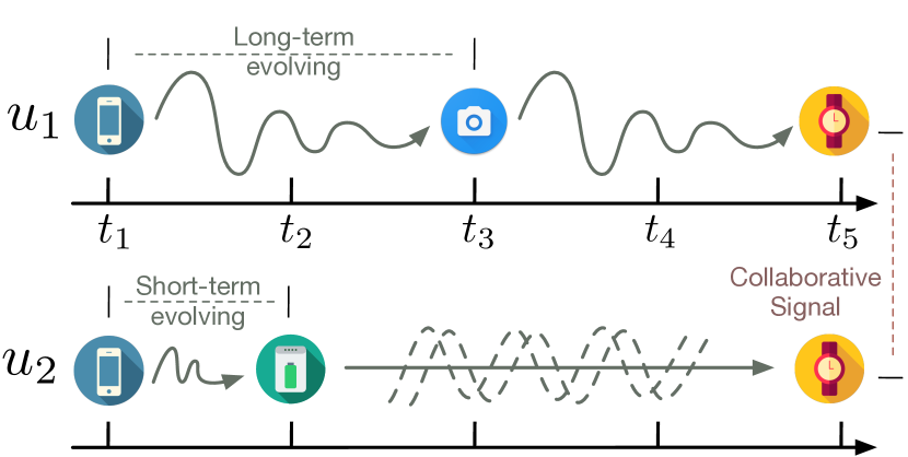
Despite the encouraging performance achieved by these SR models, most existing approaches still suffer from two key limitations: (i) Inability to model the dynamic evolution of collaborative signals. Actually, user preference is dynamic in nature. For example, a user may be interested in book items for a period of time and then search for new electronic games, and thus how to effectively model and understand the underlying dynamics becomes a critical problem. Moreover, the dynamic evolution of collaborative signals is also a crucial component in capturing user preference. Existing efforts generally predict the next item by merely modeling the item-item transitions inside sequences or capturing the interaction process in a static graph, ignoring the dynamic evolution of collaborative signals. (ii) Fail to consider irregularly-sampled intervals of the observed interactions. Most methods usually assume the observations are regularly sampled, which is impractical for many applications. As shown in Figure 1, user purchases “phonecamerawatch” at regular time intervals, we can speculate that he/she is a digital product enthusiast. However, user buys similar things at irregularly-sampled times, we may think that he/she buys a phone and power bank in a certain period of time because he/she just needs them, not because of his/her hobbies. The behavior of buying a watch much later, perhaps as a gift or for other reasons, suggests that irregularly-sampled observations could imply different user preferences. Therefore, how to explore the evolving process of successive user behaviors with irregular-sampled partial observations remains challenging. As such, we are looking for an approach that can model the dynamic evolution of collaborative signals and meanwhile overcome the irregularly-sampled observations.
Having realized the above challenges with existing SR methods, we focus on continuous-time sequential recommendation. Towards this end, this work proposes a principled graph ordinary differential equation framework named GDERec. The key idea of GDERec is to simultaneously characterize the evolutionary dynamics and adapt to irregularly-sampled observations. To achieve this goal effectively, GDERec is modeled by an autoregressive graph ODE composed of two components, which are parameterized by two tailored GNNs respectively to capture user preference from a hybrid dynamical systems view. On the one hand, we develop an ODE-based GNN to implicitly capture the temporal evolution of the user-item interaction graph. On the other hand, we design an attention-based GNN to explicitly incorporate collaborative attention to interaction signals when the interaction graph evolves over time. Further, the whole process can be optimized by alternately training two customized GNNs in an autoregressive manner to track the evolution of the underlying system from irregular observations. Our experiments show that it can largely improve the existing state-of-the-art approaches on five benchmark datasets. In a nutshell, we summarize the main contributions of this work are as follows:
-
•
General Aspects: Different from existing works in recommendation in discrete states, we explore continuous-time sequential recommendation, which remains under-explored and is able to generalize to any unseen times-tamps for future interactions.
-
•
Novel Methodologies: We propose a novel framework to alternately train two parts of our autoregressive graph ODE in a principled way, capable of modeling the evolution of collaborative signals and overcoming irregularly-sampled observations.
-
•
Multifaceted Experiments: We conduct comprehensive experiments on five benchmark datasets to evaluate the superiority as well as the functionality of the proposed approach against competitive baselines.
2 Related Work
In this section, we briefly review the related works in three aspects, namely sequential recommendation, graph neural networks, and ordinary differential equation.
2.1 Sequential Recommendation
Sequential recommendation (SR) aims to predict the next item based on the user’s historical interactions as a sequence by sorting interactions chronologically. The effectiveness of this method makes it possible to provide more timely and accurate recommendations. Existing approaches for SR can be mainly divided into markov chains (MC) [10, 11], RNN-based [13, 14, 15], and Transformer-based [17, 18, 19, 20, 21, 22]. Most traditional methods are based on MC and the main purpose is to model item-to-item transaction patterns. For example, FPMC [10] regards user behaviors as markov chains, and estimates the user preference by learning a transition graph over items. With the recent advances of deep learning, many deep SR models leverage RNNs to capture long-term sequential dependencies. For instance, GRU4Rec [13] leverages RNNs to incorporate more abundant history information for the session-based recommendation. The success of Transformer [16] inspires the adoption of the attention mechanism into SR. BERT4Rec [19] further applies deep bidirectional self-attention to model user behavior sequences. Different from these methods, our GDERec steps further and focuses on under-explored continuous-time SR, while existing methods fail to generalize to any unseen future times-tamps.
2.2 Graph Neural Networks
With the powerful capability of processing non-euclidean structured data, graph neural networks (GNNs) [23, 30, 31, 32, 33] have achieved wide attention due to their remarkable performance. The underlying idea is to update node representations using a combination of the current node’s representation and that of its neighbors following message passing schemas [34]. Recently, GNNs have shown great promise for enhancing existing SR methods [27, 35, 28, 29, 36, 37, 38]. SR-GNN [27] makes the first attempt to incorporate GNNs into the SR, and models session sequences as the graph to capture complex transitions of items. DGRec [35] leverages graph attention neural network [39] to dynamically estimate the social influences based on users’ current interests. However, most of the GNN-based recommendation methods only focus on static graph scenarios, and have shown the inability to track the evolution of collaborative signals and overcome irregularly-sampled observed interactions, while our GDERec innovatively addresses these limitations.
2.3 Ordinary Differential Equation
Neural ODE [40] has been proposed as a new paradigm for generalizing discrete deep neural networks to continuous-time scenarios. It forms a family of models that approximate the ResNet [41] architecture by using continuous-time ODEs. Due to the superior performance and flexible capability, neural ODEs have been widely adopted in various research fields, such as traffic flow forecasting [42, 43, 44, 45], time series forecasting [46, 47, 48], and continuous dynamical system [49, 50, 51]. Recently, there are some advanced methods connecting GNNs and neural ODEs [52, 53]. GODE [52] generalizes the concept of continuous-depth models to graphs, and parameterizes the derivative of hidden node states with GNNs. Compared with existing ODE methods, our work goes further and extends this idea to investigate an under-explored yet important continuous-time sequential recommendation.
3 Preliminary
As the fundamental recommendation problem, sequential recommendation system aims to predict the preference of users based on the observed historical user-item interaction sequences. Graph neural network (GNN) based recommendation approaches have been proposed to represent the interaction between users and items as a bipartite graph. Specifically, let and be the sets of users and items respectively, the temporal interaction bipartite graph is formulated as , where denotes the vertices set and is the temporal edge set denoting the observed interactions.
Since the observed interactions have taken place in the temporal order, given a set of pivot timestamps , we can consequently define the hybrid time domain by dividing the continuous time domain into different slices separated by the pivot timestamps. The interaction stream on the graph can be further viewed as a hybrid dynamic system , where each
| (1) |
The construction of depicts the hybrid dynamic process of a given interaction system by representing the continuous evolution process between pivot timestamps and the discrete instant influence of interactions at each pivot . Since we have constructed the system, the object of GNN-based sequential recommendation is to predict the interactions during next period , given the interaction graph . Additionally, to fully leverage the hybrid dynamic of the system, the method is expected to be capable of handling both the continuous evolution within time slices and the sudden changes at discrete time pivots.
4 Methodology
4.1 Overview
In this paper, we introduce our approach for continuous-time sequential recommendation by incorporating the evolutionary dynamics of underlying systems. Existing methods merely explore the sequential patterns and model item transitions assuming uniform intervals. However, they are not able to fully capture the evolution of collaborative signals and fail to adapt to irregularly-sampled observations, which leads to insufficient expressiveness.
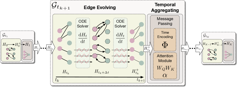
We address the above limitations by proposing a novel graph ordinary differential equation framework called GDERec. Specifically, GDERec builds a principled autoregressive graph ODE consisting of two parameterized GNNs. On the one hand, a tailored ODE-based GNN is developed to implicitly track the temporal evolution of collaborative signals on the user-item interaction graph. On the other hand, we leverage the attention mechanisms to equip GNN to explicitly capture the evolving interactions when the interaction graph evolves over time. The two components are trained alternately to learn effective representations of users and items beneficial to the recommender system. An illustration of the framework is presented in Figure 2. Next, we will introduce the edge evolving module and the temporal aggregating module. Finally, the training algorithm to optimize the model is explained.
4.2 Edge Evolving Module
GNNs propagate and aggregate messages on given graph adjacency structures. Typically, graph convolution layers take the form of the following message passing scheme:
| (2) |
where denotes the hidden representation of nodes on the -th layer and is the initial node embeddings. represents the normalized graph adjacency matrix. The message function of GCNs weights the influence of neighborhood by the normalized node degrees, which ignores the natural affinity between connected nodes. However, the user would receive different influences from the interacted items. Towards this end, we follow the advice of previous work [54] and rewrite the propagation process:
| (3) |
where the first item in the message function represents the standard message passed via graph convolution, while the second item takes the form of the element-wise product of the source and the destination nodes’ representations to model the affinity between neighboring nodes.
Specifically, in recommendation scenarios, user preference and item representation would evolve with the continuous-time flow. In other words, it requires the extent of the discrete propagation to continuous form to further simulate the temporal evolution process on a dynamic graph. Intuitively, we can expand Eq. 3 as:
| (4) | ||||
From Eq. 4 we can obtain the closed-form solution of neighborhood propagation with arbitrary number of layers. To get more fine-grained representations of the interaction graph, we hope to extend Eq. 4 to continuous form. Specifically, we replace the discrete with a continuous variable and Eq. 4 can thus be viewed as a Riemann sum. We have the integral formulation:
| (5) |
However, the item is intractable to compute for . Therefore we aim to reform the calculation of as an ordinary differential equation and state the following propositions to elicit the numerical solution of .
Proposition 1 The first-order derivative of in Eq. 5 can be formulated as the following ODE:
| (6) |
where the initial is the output from downstream networks.
Proof 4.1
We first directly calculate the derivative of as:
| (7) |
To get rid of the remaining items with , We further calculate the second-order derivative of :
| (8) | ||||
By integration on both sides of Eq. 8, we have:
| (9) |
To solve the value of , we let and combine Eq. 7 and 9:
| (10) |
We get that:
| (11) |
and the derivative form of the ODE process can be rewritten as:
| (12) |
So far we have obtained the first order derivative of with respective to time variable that is only determined by the value of , the initial representation matrix , and the normalized adjacency . The formulation of Eq. 12 can be further fed into neural ODE frameworks [40] to model the evolving process of .
To calculate in practice, we approximate it by making a first-order Taylor approximation to .
| (13) |
Specifically, the ODE we propose has an analytical solution.
Proposition 2 The analytical solution of Eq. 13 is given by:
| (14) |
Proof 4.2
To solve the ODE defined by Eq. 13, we first multiply both sides of the equation by an exponential factor and rearrange the items:
| (15) |
By integrating from 0 to a specified on both side, we can thus obtain by the integral results:
| (16) |
where the item S is given by:
| (17) |
From Eq. 16 we obtain for any :
| (18) | ||||
where the analytical solution of is given by:
| (19) |
Since we have modeled the discrete dynamics in Eq. 13 of evolving interacting system in an ODE formulation, the value of given a continuous time can then be solved by a designated ODE solver such as Runge–Kutta method [55]:
| (20) |
For fixed step size , a typical ODE solver would iteratively update the value of . For instance, to solve an initial value problem of ODEs that formulated as:
| (21) |
where represents in our case. The Runge-Kutta-4 (RK-4) solver updates the value with:
| (22) | ||||
4.3 Temporal Aggregating Module
Recalling that the constructed hybrid dynamic system in Eq. 1 is composed of the continuous intervals between pivot times and the discrete pivot timestamps. While the edge evolving module models the continuously evolving process between any and , we design a temporal aggregating module to explicitly aggregate neighboring information on a given interaction graph. For instance, given the temporal edges , which represents the interactions before , and the node representations calculated in Eq. 20, our goal is to obtain a propagation function F:
| (23) |
where is the output representation of the current layer, denotes trainable network parameters.
4.3.1 Trainable Time Encoding
To explicitly encode temporal information presented in the temporal edges, we propose to introduce a time mapping that maps a given timestamp into the latent space. Previous researches [56] proposed several translation-invariant time encoding functions, i.e., that satisfy:
| (24) |
where denotes the inner product of two given vectors. Here we implicate Bochner’s theorem [57] as our time encoding function:
| (25) |
where is the trainable time embedding to reflect flexible temporal characteristics.
4.3.2 Temporal Attention Network
Graph attention networks [39] suggest leveraging the target attention mechanism in the message function. To incorporate temporal factors into the attention mechanism, we propose to build an attention network that jointly captures chronological and contextual information. Particularly, given the hidden representation of the previous layer and temporal edges , the message passed from arbitrary node to node at -th layer is constructed as:
| (26) |
where represents the passed message. For target node , denotes the neighboring node of in . We follow GCNs [23] and apply the Laplacian normalization to each node to avoid the over-squashing issue on the large user-item graph. The attention weight is calculated via the soft-attention mechanism to model the characterized contribution from the neighborhood to each node:
| (27) |
where are all trainable attention parameters, denotes sigmoid function:
| (28) |
4.4 Autoregressive Propagation Module
Since we have defined the formulation of the edge evolving module and the temporal aggregating module, given an interaction graph , we can build the corresponding hybrid dynamic interacting system and the initial node embeddings . We design an autoregressive framework that propagates messages on the hybrid dynamic time domain. To formulate, we have:
| (29) |
where are list of model parameters.
So far we have defined the whole propagation process on a given hybrid dynamic interacting system, where the graph ODE-based module steers the evolving dynamics of the interacting process and calculates for each layer, and then the message-passing-based module explicitly models the temporal factors via a tailored temporal attention mechanism to output for next period of time. GDERec obtains layers of hidden representations by applying these two modules autoregressively as formulated in Eq. 29.
4.5 Model Prediction and Optimization
After iteratively propagating along the hybrid dynamic interacting system , we can obtain the hidden representation of nodes on each layer, namely , where for each layer we have . For a given user-item pair , we obtain the corresponding node representation via:
| (30) |
To model the preference for the designated user to target item , we calculate the rating score by the inner product of representations:
| (31) |
To optimize the model parameters, we adapt Bayesian Personalized Ranking (BPR) [58] loss as the target function, formulated as:
| (32) |
where denotes the involved model parameters and node embeddings, . For each iteration, we randomly sample the negative interaction set from .
Complexity Analysis. Following the autoregressive propagation schema defined in previous sections, the computational consumption is mainly composed of two parts: (i) the ODE solver that estimates the solution of the proposed graph ODEs; (ii) the graph propagation process that aggregates node features on graphs.
For (i), there are several kinds of numerical methods to solve a given ordinary differential equation, for example, fixed-step methods like Runge-Kutta method [55] and adaptive-step methods like Dormand-Prince-Shampine method [59]. In this work, we choose the Runge-Kutta-s algorithm to solve the ODE with a fixed step of -th order. Thus for a fixed step size , the total time complexity of the solving process can be calculated via:
| (33) |
For (ii), the complexity of the edge propagation is only determined by the number of edges and the size of node representation:
| (34) |
To sum up, we have the overall complexity of GDERec:
| (35) |
4.6 Comparison with Existing Models
As a graph-based ODE model, GDERec is related to several existing methods that includes:
-
•
LightGCN [60]: LightGCN is a classical graph convolution-based approach that conducts normalized graph convolution on the user-item interaction graph. Nonetheless, it overlooks the temporal disparities among interactions and the evolution of user interests. In contrast, our GDERec extends the utility of interaction graphs by introducing the concept of a hybrid dynamic system and a graph ODE network, which enable us to model the continuous evolution of user interests.
-
•
GNG-ODE [61]: GNG-ODE is a session graph-based recommendation method that integrates neural ODEs with session graphs. Specifically, GNG-ODE captures the evolving dynamics of users by proposing the t-Alignment technique, which enables the session graph to expand over time, which is similar to our proposed hybrid dynamic system. However, GNG-ODE only performs graph encoders on session graphs, thereby neglecting the evolving collaborative signals between users and items. In contrast, our GDERec enhances the interaction system by incorporating time-evolving interaction edges. This hybrid dynamics facilitates the model’s reception of more finely-grained global collaborative signals.
In summary, our GDERec stands out as the first endeavor to integrate interaction dynamics into continuous-time recommendations, leveraging the novel hybrid dynamic systems and an ODE-based autoregressive propagation approach. The subsequent sections will provide empirical evidence of the effectiveness of our GDERec
5 Experiment
We conduct comprehensive experiments on several benchmark datasets to evaluate the effectiveness of the proposed GDERec and answer the following research questions.
RQ1: How does the proposed GDERec perform on real-world datasets compared with the current state-of-art methods? Is the idea of modeling hybrid dynamics effective for recommendations?
RQ2: How does the idea of the hybrid dynamic interaction system enhance the recommendations? How do the hyper-parameters influence GDERec’s performance?
RQ3: Can GDERec capture dynamic features of the interactions effectively as time flows? Is there a way to visualize the learned dynamics system in the hidden space?
5.1 Overall Comparison (RQ1)
5.1.1 Datasets and Experimental Setup
| Dataset | #User | #Item | #Interactions | Density |
| Cloth | 39,387 | 23,033 | 278,677 | 0.31% |
| Baby | 19,445 | 7,050 | 160,792 | 0.11% |
| Music | 5,541 | 3,568 | 64,706 | 0.32% |
| ML-1M | 6,040 | 3,706 | 1,000,209 | 4.46% |
| ML-100K | 943 | 1,682 | 100,000 | 6.30% |
We evaluate GDERec and baseline methods on five real-world datasets, including three subsets of the Amazon review dataset111https://jmcauley.ucsd.edu/data/amazon/, namely Electronics, Cloth, and Music, and two subsets of the Movie-Lens dataset222https://grouplens.org/datasets/movielens/, namely ML-1M and ML-100K. The detailed statistics of the used datasets are presented in table I. The observed interactions in each dataset are chronologically sorted by the timestamp and then split into train/valid/test sets by an 80%/10%/10% ratio, which is a common practice.
For GDERec, we construct the hybrid interaction system for each dataset by averagely splitting the time interval of the dataset into time slots from the earliest click to the latest, defined by pivot timestamps: . During the experiment, the number of intervals is searched from .
5.1.2 Compared Baselines
| Model | Cloth | Baby | Music | ML-1M | ML-100K | ||||||||||
|---|---|---|---|---|---|---|---|---|---|---|---|---|---|---|---|
| R@5 | R@10 | MRR | R@5 | R@10 | MRR | R@5 | R@10 | MRR | R@5 | R@10 | MRR | R@5 | R@10 | MRR | |
| GRU4Rec | 0.0106 | 0.0212 | 0.0090 | 0.0295 | 0.0521 | 0.0219 | 0.0375 | 0.0544 | 0.0216 | 0.1065 | 0.2131 | 0.0755 | 0.1769 | 0.3475 | 0.1136 |
| SASRec | 0.0115 | 0.0206 | 0.0099 | 0.0309 | 0.0548 | 0.0215 | 0.0429 | 0.0771 | 0.0320 | 0.1010 | 0.2135 | 0.0787 | 0.1675 | 0.3064 | 0.1050 |
| TiSASRec | 0.0112 | 0.0214 | 0.0106 | 0.0318 | 0.0557 | 0.0234 | 0.0510 | 0.0825 | 0.0322 | 0.1121 | 0.2253 | 0.0778 | 0.1792 | 0.3552 | 0.1108 |
| SR-GNN | 0.0058 | 0.0103 | 0.0045 | 0.0140 | 0.0276 | 0.0115 | 0.0359 | 0.0650 | 0.0295 | 0.1091 | 0.2187 | 0.0744 | 0.1781 | 0.3422 | 0.1011 |
| LightGCN | 0.0169 | 0.0283 | 0.0106 | 0.0325 | 0.0537 | 0.0233 | 0.0642 | 0.1167 | 0.0451 | 0.1079 | 0.2214 | 0.0757 | 0.1676 | 0.3128 | 0.1028 |
| DGCF | 0.0170 | 0.0289 | 0.0112 | 0.0289 | 0.0518 | 0.0213 | 0.0695 | 0.1258 | 0.0459 | 0.1151 | 0.2276 | 0.0789 | 0.1601 | 0.3329 | 0.1062 |
| IOCRec | 0.0129 | 0.0264 | 0.0115 | 0.0329 | 0.0542 | 0.0229 | 0.0649 | 0.1178 | 0.0440 | 0.1149 | 0.2259 | 0.0772 | 0.1855 | 0.3622 | 0.1175 |
| DCRec | 0.0117 | 0.0251 | 0.0108 | 0.0335 | 0.0551 | 0.0227 | 0.0591 | 0.1062 | 0.0433 | 0.1160 | 0.2285 | 0.0791 | 0.1802 | 0.3541 | 0.1162 |
| TGSRec | 0.0104 | 0.0271 | 0.0114 | 0.0142 | 0.0240 | 0.0116 | 0.0243 | 0.0377 | 0.0158 | 0.1109 | 0.2123 | 0.0749 | 0.1601 | 0.3277 | 0.1120 |
| NODE | 0.0184 | 0.0293 | 0.0117 | 0.0339 | 0.0525 | 0.0224 | 0.0584 | 0.0967 | 0.0420 | 0.1148 | 0.2297 | 0.0785 | 0.1739 | 0.3404 | 0.1098 |
| GCG-ODE | 0.0186 | 0.0299 | 0.0123 | 0.0340 | 0.0558 | 0.0238 | 0.0682 | 0.1237 | 0.0455 | 0.1149 | 0.2263 | 0.0767 | 0.1846 | 0.3598 | 0.1161 |
| GDERec | 0.0198 | 0.0331 | 0.0146 | 0.0351 | 0.0577 | 0.0256 | 0.0738 | 0.1363 | 0.0528 | 0.1210 | 0.2389 | 0.0801 | 0.1919 | 0.3712 | 0.1197 |
To demonstrate the effectiveness of our work, we compare GDERec with the current state-of-the-art baseline methods. Specifically, we choose the baseline methods from three different perspectives: (a) sequence-based recommendation(SR) models; (b) graph-based collaborative filtering methods; (c) continuous-time recommendation methods; (d) contrastive learning-based recommendation models.
-
•
(a) GRU4Rec [13]: A SR model that leverages Recurrent Neural Networks (RNNs) to make predictions.
-
•
(a) SASRec [18]: A transformer-based SR model that introduces attention mechanism into recommendations.
-
•
(a) TiSASRec [62]: A variant of SASRec that takes time intervals between interactions into consideration. It is one of the state-of-the-art attention-based SR baselines.
-
•
(b) SR-GNN [27]: A gated graph neural network (GGNN)-based session recommendation method.
-
•
(b) LightGCN [60]: A classic GNN-based collaborative filtering method that uses GCNs in recommendation tasks.
-
•
(b) DGCF [63]: It is a variant of LightGCN, which introduces disentangled representation learning into collaborative filtering. It’s one of the state-of-the-art graph recommendation models.
-
•
(c) TGSRec [21]: A dynamic temporal graph-based model that integrates transformer with graph recommendations.
-
•
(c) NODE [64]: A neural ordinary differential equation (NODE)-based recommendation method that combines neural ODE with LSTMs to make sequence-based recommendations.
-
•
(c) GNG-ODE [61]: A graph-based model that depicts the continuous-time session graphs with neural ODEs.
-
•
(d) IOCRec [65]: A sequence based contrastive learning approach that focuses on the intent-level self-supervision signals to promote model performance.
-
•
(d) DCRec [66]: A contrastive-based model that unifies sequential pattern encoding with global collaborative relation modeling in sequence recommendation.
5.1.3 Model Settings
When evaluating our GDERec as well as all the compared baselines, we fix the embedding size for the user and items as 64 and the embedding size for the trainable time encoding vector as 16 if used. All models are optimized with the learning rate fixed . For a fair comparison, we utilize the same L2 normalization with fixed . The max sequence length for sequence-based models is fixed at 50. Specifically, the step size of the Runge-Kutta method for ODE-based models (GDERec, NODE) is fixed as . Specifically, for interaction graph-based methods (LightGCN, DGCF and TGSRec), we obtain the user-item graph from the interactions within the train set, and the number graph propagation layers is searched from . The number of disentanglement of DGCF is searched from . For TGSRec, we sample temporal neighbors at each layer of temporal graph. All of the mentioned methods are implemented using PyTorch and torchdiffeq333https://github.com/rtqichen/torchdiffeq.
To evaluate the model performance, we adopt Recall@K and MRR as the evaluation metrics, following the advice of previous works [21, 64]. To be specific, we calculate Recall@5, Recall@10 and MRR along with all the items ranked by the model. The model that achieves the highest MRR on the evaluation set is selected to be tested on the test set and the test results are shown in table II.
5.1.4 Experimental Results
From the results reported in table II, we can make the following observations:
-
•
User-item graph-based baseline methods (LightGCN and DGCF) outperform sequence-based methods when the datasets are rather sparse (i.e. Cloth, and Music), where the high-order similarities between users and items can provide useful information. On the other hand, sequence-based models (GRU4Rec, SASRec, and TiSASRec) yield better results on dense datasets. Specifically, contrastive learning-based method (IOCRec and DCRec) shows more competitive performance, which demonstrates the effectiveness of contrastively learning to represent items.
-
•
ODE-based methods ( NODE, GNG-ODE and GDERec) generally achieve promising performance on both sparse and dense datasets, which shows the effectiveness of depicting the continuous dynamics of user behaviors. Neural ODE helps to overcome the difficulties brought by irregularly sampled interactions, as well as to capture the implicit dynamics in long-term interacting systems.
-
•
GDERec outperforms all baseline methods on all datasets. In particular, GDERec has gained more than and relative improvement at Recall@5 and Recall@10, as well as a relative improvement at MRR. The improvement made by GDERec benefited from building a hybrid dynamic interaction system and a well-designed graph propagation scheme.
5.2 Ablation and Parameter Studies (RQ2)
In this section, we further investigate the detailed functionality of different modules in GDERec, as well as their performance under various kinds of input temporal signals by conducting ablation studies. We will also explore GDERec’s sensitivity to the hyper-parameters.
5.2.1 Functionality of Graph Modules
| Dataset | Cloth | Baby | Music | ML-1M | ML-100K | ||||||||||
|---|---|---|---|---|---|---|---|---|---|---|---|---|---|---|---|
| R@5 | R@10 | MRR | R@5 | R@10 | MRR | R@5 | R@10 | MRR | R@5 | R@10 | MRR | R@5 | R@10 | MRR | |
| LightGCN | 0.0169 | 0.0283 | 0.0106 | 0.0325 | 0.0537 | 0.0233 | 0.0642 | 0.1167 | 0.0451 | 0.1079 | 0.2214 | 0.0757 | 0.1676 | 0.3128 | 0.1028 |
| GDERecATT | 0.0160 | 0.0279 | 0.0113 | 0.0317 | 0.0533 | 0.0229 | 0.0641 | 0.1178 | 0.0461 | 0.1132 | 0.2211 | 0.0768 | 0.1909 | 0.3733 | 0.1138 |
| GDERecODE | 0.0173 | 0.0295 | 0.0125 | 0.0323 | 0.0565 | 0.0245 | 0.0693 | 0.1280 | 0.0519 | 0.1061 | 0.2243 | 0.0746 | 0.1739 | 0.3571 | 0.1095 |
| GDERecGCN | 0.0187 | 0.0303 | 0.0134 | 0.0349 | 0.0574 | 0.0260 | 0.0707 | 0.1291 | 0.0506 | 0.1192 | 0.2388 | 0.0799 | 0.1887 | 0.3690 | 0.1101 |
| GDERec | 0.0198 | 0.0331 | 0.0146 | 0.0351 | 0.0577 | 0.0256 | 0.0738 | 0.1363 | 0.0528 | 0.1210 | 0.2389 | 0.0801 | 0.1919 | 0.3712 | 0.1197 |
Since we have proposed two different graph propagation schemes: an ODE-based edge evolving module and an attention-based temporal aggregating module, it’s necessary to conduct ablation studies to demonstrate the effectiveness of the two tailored-designed propagation modules. To be specific, we consider the following variants of GDERec to explore how both modules cooperate for better recommendation results.
To start with, we test the model performance by removing the temporal attention module and replacing the module with the plain Graph Convolution Networks (GCNs) respectively to verify the effectiveness of the temporal aggregating module, namely GDERecODE and GDERecGCN. Then we remove the edge evolving module from the original model, namely GDERecAtt. From the results in Table III we can observe that:
-
•
Both the edge evolving module and temporal aggregating module are important for GDERec to achieve better performance. Specifically, GDERecATT suffers the most performance decline for removing the ODE layers from the original architecture.
-
•
The comparison between GDERec and GDERecGCN demonstrates the superiority of our proposed temporal attention module over regular graph convolutions. GDERec outperforms more over GDERecGCN on datasets that include longer time spans (i.e. Cloth, Music), rather than datasets within a relatively short time period (ML-1M). The result reveals the strength of GDERec in dealing with long-term interacting systems.
5.2.2 Influence of Temporal Encoding
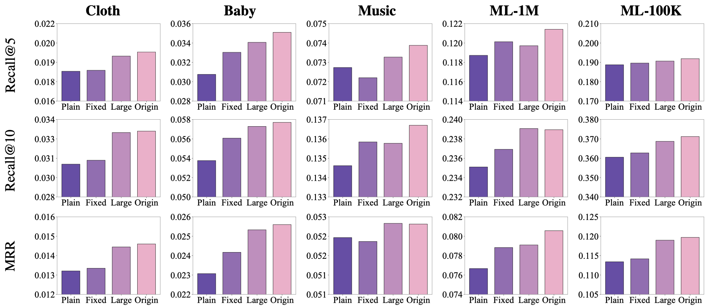
In the attention module, a set of learnable time encoding functions have been defined in Eq. 25 to bring more temporal information to the module. To validate the effectiveness of the proposed encoding functions, we conduct a series of ablation studies by replacing the attention module with (a) a plain attention module without temporal encodings, (b) temporal encodings with fixed random weights, (c) default temporal encodings with , and (d) extreme large temporal encodings with . As illustrated in Figure 3, we observe that:
-
•
Time encodings are necessary for GDERec to better leverage temporal information. In general, the plain attention method without time encodings would lead to sub-optimal results.
-
•
In most cases, learnable time encodings are better than fixed parameters for self-adapting to flexible time spans. However, extremely large time vectors could lead noises into attention modules and cause a performance decline.
5.2.3 Influence of System Dynamic
| Method | Input Signal | Cloth | Baby | Music | ML-1M | |||||||||
|---|---|---|---|---|---|---|---|---|---|---|---|---|---|---|
| ODE | Attn. | R@5 | R@10 | MRR | R@5 | R@10 | MRR | R@5 | R@10 | MRR | R@5 | R@10 | MRR | |
| All | All | 0.0181 | 0.0321 | 0.0133 | 0.0338 | 0.0523 | 0.0238 | 0.0687 | 0.1233 | 0.0502 | 0.1108 | 0.2217 | 0.0769 | |
| Cur. | Cur. | 0.0185 | 0.0332 | 0.0137 | 0.0336 | 0.0570 | 0.0253 | 0.0728 | 0.1296 | 0.0511 | 0.1251 | 0.2280 | 0.0783 | |
| Prev. | Cur. | 0.0182 | 0.0336 | 0.0132 | 0.0330 | 0.0549 | 0.0241 | 0.0679 | 0.0128 | 0.0494 | 0.1201 | 0.2377 | 0.0784 | |
| Prev. | Prev. | 0.1783 | 0.0309 | 0.0126 | 0.0312 | 0.0538 | 0.0229 | 0.0715 | 0.1278 | 0.0517 | 0.1207 | 0.2397 | 0.0783 | |
| Origin | Cur. | Prev. | 0.0198 | 0.0331 | 0.0146 | 0.0351 | 0.0577 | 0.0256 | 0.0738 | 0.1363 | 0.0528 | 0.1210 | 0.2389 | 0.0801 |
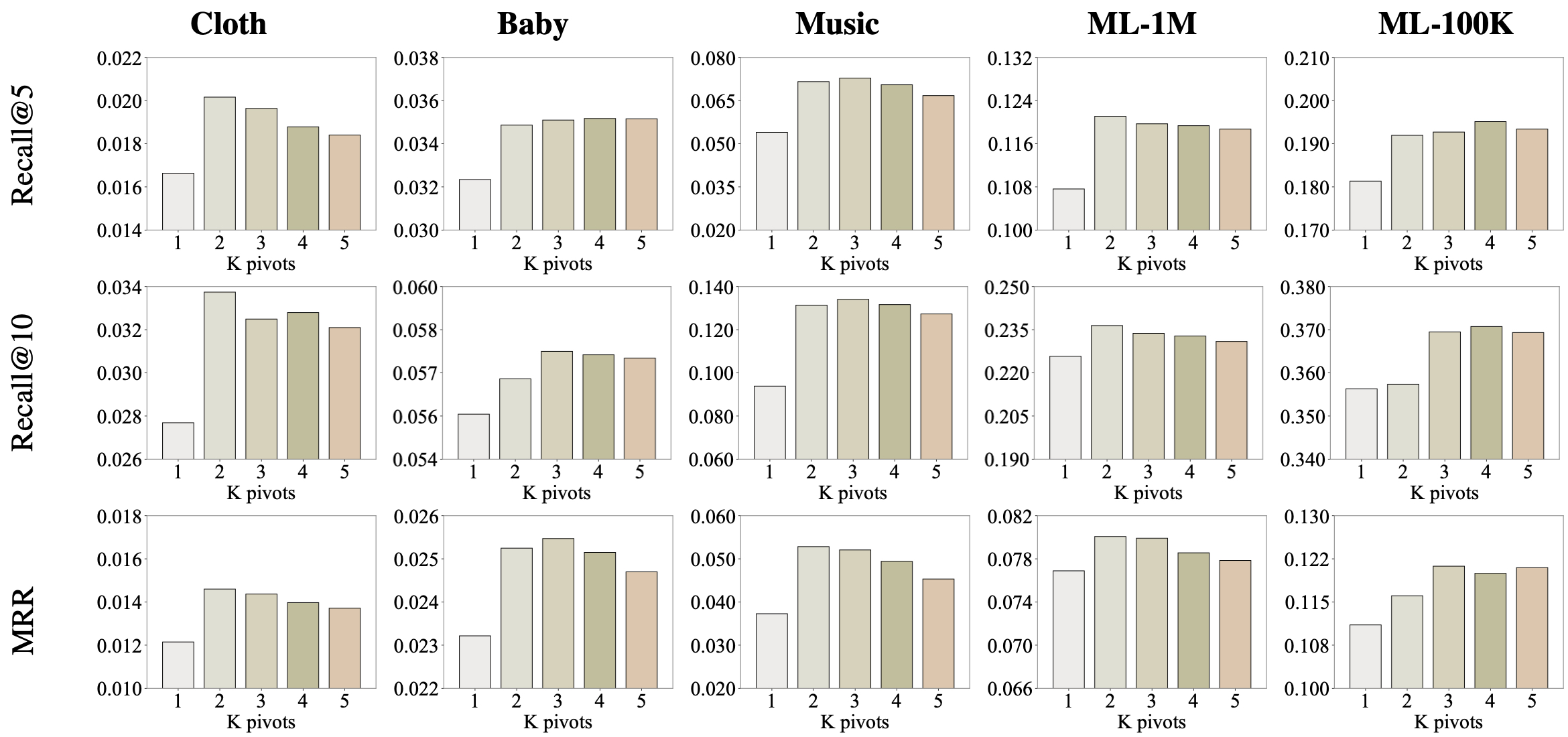
Recalling that we build a hybrid dynamic interaction system based on the time interval of the original interaction dataset, thus the system dynamic is influenced by the defined pivot timestamps . To be specific, by increasing , we are adding more pivot timestamps to the system and thus introducing more detailed dynamic features for GDERec in the ODE-based edge evolving process. From the results illustrated in Figure 4, we can observe that:
-
•
By setting a larger , the model could benefit from the detailed dynamics of the interacting system. Generally, the performance of GDERec reaches the optimal when is set by 3 as a trade-off between performance and computational cost.
-
•
Too many time intervals (more than 4) may cause a decline in the model performance on both datasets.
5.2.4 Model’s Sensitivity to Temporal Signals
In GDERec, the interactions between users and items are split into a set of hybrid dynamic systems . By default, the two components of the autoregressive framework defined in Eq. 29 receive interactions with different temporal signals. Specifically, the edge evolving module is concerned about the interactions within just the current time interval, while the temporal aggregating module would aggregate the neighbors that belong to current or previous intervals.
However, we wonder if this set of input temporal signals can fully exploit the potential of GDERec’s autoregressive framework to better leverage the dynamics in an interacting system. Thus we conduct experiments on GDERec with different combinations of input signals, listed as follows:
-
1.
. Static System: The ODE module and the attention module would both receive all observed interactions as input.
-
2.
. Short-sighted Model: Both modules are limited to using only the interactions within the current interval.
-
3.
. Reversed Sights: In contrast to the original setting, the ODE module can take previous interactions as input and the attention module is limited to only the current interval.
-
4.
. Look-back Model: Both modules now can leverage interactions from history so far.
The experimental results are illustrated in table IV of all the mentioned methods, comparing with the original modal. We can observe from the results that:
-
•
In most cases, compared with static interactions as inputs (), inputs with different degrees of dynamic signals (-) show better performance, which demonstrates that it is necessary to introduce dynamic temporal signals.
-
•
Compared with other combinations, the original input of GDERec stays stable advantage on all datasets. On the one hand, the ODE module would receive only the latest interactions and thus avoid the overloaded information brought by previous long sequences and depict the fine-grained interaction dynamics. On the other hand, the attention module could leverage all historical information to adaptively respond to the growing interaction graph.
5.2.5 Influence of Model Depth
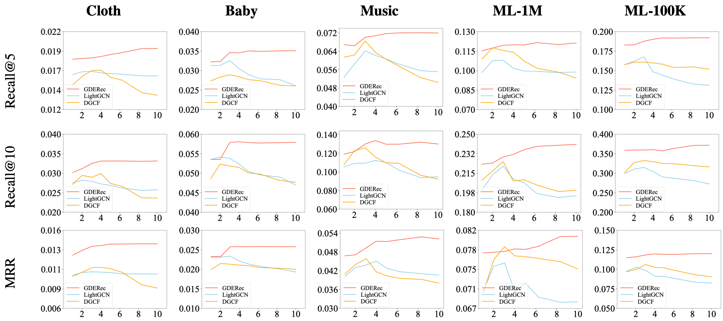
As one of the advantages of neural ODEs, we can extend the model depth by controlling the number of function evaluations (NFE) of the numerical ODE solver, without concerns about the over-smoothing issue brought by GNN layers. In particular, we vary the model depth from 1 (discrete form) to 10 with fixed to validate the influence of the depth of the edge evolving module. We conduct experiments on the Music dataset and from the results shown in Figure 5 we can observe that:
-
•
With the increase in model depth, GNN-based models (LightGCN and DGCF) will suffer from the over-smoothing issue and the decline in performance. On the other hand, ODE-based GDERec benefits from increasing the model depth, indicating the capability of Neural ODEs to capture the long-term evolving features.
-
•
When the model becomes deeper, the performance of GDERec will firstly reach the optimal and then maintain stable performance, showing its robustness to exploit dynamic interactions. However, the growth of model performance slows down when the model is too deep (more than 6 layers), where stacking more layers could gain little performance growth.
5.3 Visualization and Case Study (RQ3)
Since we have proposed to model the dynamic factors to model an irregularly-sampled interaction system, we attempt to understand how users and items evolve as GDERec propagates. Towards this end, we randomly choose a user from the ML-1M dataset and visualize the hidden representation of as well as the clicked movies during different periods and conduct a series of studies to investigate how GDERec alleviate the irregularly-sampled issue.
5.3.1 Visualization of Temporal Attention
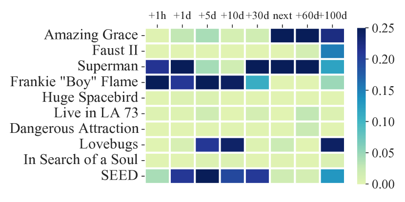
The use of temporal encodings in the attention module brings fine-grained temporal information, which helps the model respond to different time conditions. Specifically, we choose a random user from the amazon-music dataset and sampled 10 songs from his historical clicks. We obtain the output logits on these songs of the attention module, followed by a soft-max normalization, and visualize them in a heat map in Figure 6. Each row represents a time increment since the first interaction of the user, and row ”next” represents the day when the test set begins. From the figure, we can observe the dynamic evolution of user interest and the temporal encodings empower the attention module to capture the fluid interests.
5.3.2 Case Study on Hybrid Dynamic System
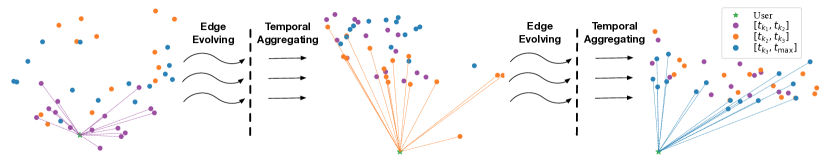
As the hidden representations evolve as time proceeds, we attempt to visualize the influence of the temporal factors in the node embedding space. To be specific, we visualize the hidden representation of and the movies he/she has clicked on each period to illustrate how the embedding space of irregularly-sampled items evolves with the dynamic interaction system. We use the t-SNE algorithm [67] to visualize the representations of movies being clicked in different periods, which are marked with corresponding colors, as shown in Figure 7.
As illustrated in Figure 7, we can observe the cluster structure of the interacted items during different time periods. The distance between the user (marked with green stars) and items (marked with corresponding colored dots) changes over time periods, reflecting the effects of the edge evolving module. The interactions generate attractive forces between users and items and the neural ODE process depicts this evolution effect in the embedding space. The visualization illustrates GDERec can encode items sampled at irregular timestamps and depict the dynamic evolution in the latent space.
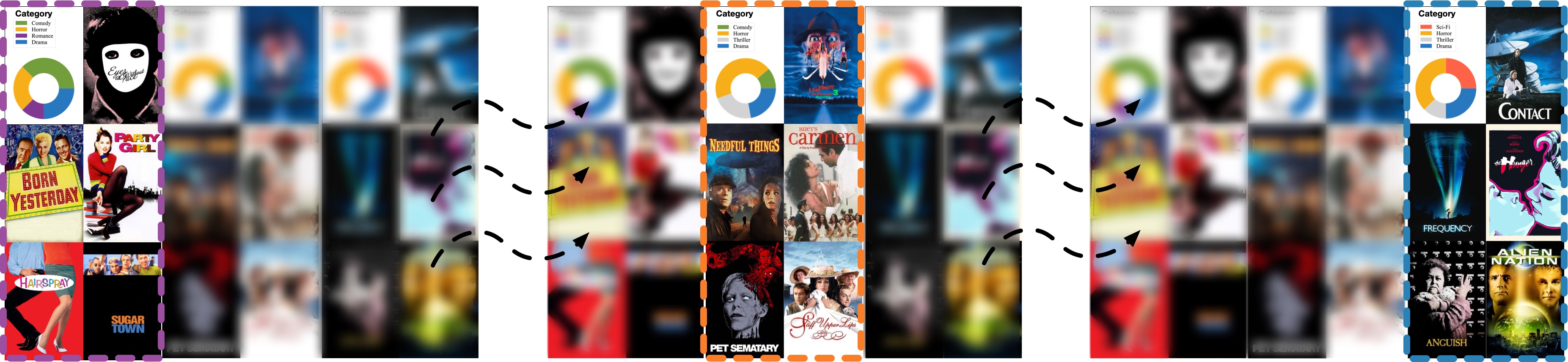
We further show parts of the movies has rated444The movie posters are downloaded from MovieLens website https://movielens.org. during different time periods in Figure 8. By arranging the rated movies in temporal order, we can observe the favorable change of in different movie categories. During the first period preferred comedies and dramas, before his/her taste gradually changed to horror films and thrillers in the second period, and during the last period of time, is shown to develop new interests in Sci-Fis. Compared with the visualization in Figure 7, we can observe that GDERec has successfully learned the temporal preference of , and the evolving process is reflected by the item embeddings.
6 Conclusion
In this work, we propose an autoregressive ODE-based graph recommendation framework GDERec, for graph recommendation on the hybrid dynamic interacting system, which is built upon two tailored designed graph propagation modules. On the one hand, a neural ODE-based edge evolving module implicitly depicts the dynamic evolving process brought by the collaborative affinity between user-item interactions. On the other hand, a temporal attention-based graph aggregating module explicitly aggregates neighboring information on the interaction graph. We define the way to build the corresponding hybrid dynamic interaction systems given a temporal interaction graph . By autoregressively applying the two modules, GDERec obtains node representations with temporal and dynamic features on a hybrid dynamic system. Comprehensive experiments and visualization results on several real-world datasets illustrate the effectiveness and strength of GDERec.
Acknowledgments
The authors are grateful to the anonymous reviewers for critically reading this article and for giving important suggestions to improve this article.
This paper is partially supported by National Key Research and Development Program of China with Grant No. 2023YFC3341203, the National Natural Science Foundation of China (NSFC Grant Numbers 62306014 and 62276002) as well as the China Postdoctoral Science Foundation with Grant No. 2023M730057.
References
- [1] J. Wang, P. Huang, H. Zhao, Z. Zhang, B. Zhao, and D. L. Lee, “Billion-scale commodity embedding for e-commerce recommendation in alibaba,” in Proceedings of the 24th ACM SIGKDD International Conference on Knowledge Discovery & Data Mining, 2018, pp. 839–848.
- [2] Z. Li, X. Shen, Y. Jiao, X. Pan, P. Zou, X. Meng, C. Yao, and J. Bu, “Hierarchical bipartite graph neural networks: Towards large-scale e-commerce applications,” in 2020 IEEE 36th International Conference on Data Engineering (ICDE). IEEE, 2020, pp. 1677–1688.
- [3] X. Zhang, C. Zhang, X. Li, X. L. Dong, J. Shang, C. Faloutsos, and J. Han, “Oa-mine: Open-world attribute mining for e-commerce products with weak supervision,” in Proceedings of the ACM Web Conference 2022, 2022, pp. 3153–3161.
- [4] E. Min, Y. Rong, Y. Bian, T. Xu, P. Zhao, J. Huang, and S. Ananiadou, “Divide-and-conquer: Post-user interaction network for fake news detection on social media,” in Proceedings of the ACM Web Conference 2022, 2022, pp. 1148–1158.
- [5] M. Mousavi, H. Davulcu, M. Ahmadi, R. Axelrod, R. Davis, and S. Atran, “Effective messaging on social media: What makes online content go viral?” in Proceedings of the ACM Web Conference 2022, 2022, pp. 2957–2966.
- [6] J. Song, K. Han, and S.-W. Kim, ““i have no text in my post”: Using visual hints to model user emotions in social media,” in Proceedings of the ACM Web Conference 2022, 2022, pp. 2888–2896.
- [7] A. Mnih and R. R. Salakhutdinov, “Probabilistic matrix factorization,” Advances in neural information processing systems, vol. 20, 2007.
- [8] P. Gopalan, J. M. Hofman, and D. M. Blei, “Scalable recommendation with hierarchical poisson factorization.” in UAI, 2015, pp. 326–335.
- [9] Y. Koren, R. Bell, and C. Volinsky, “Matrix factorization techniques for recommender systems,” Computer, vol. 42, no. 8, pp. 30–37, 2009.
- [10] S. Rendle, C. Freudenthaler, and L. Schmidt-Thieme, “Factorizing personalized markov chains for next-basket recommendation,” in Proceedings of the 19th international conference on World wide web, 2010, pp. 811–820.
- [11] R. He and J. McAuley, “Fusing similarity models with markov chains for sparse sequential recommendation,” in 2016 IEEE 16th international conference on data mining (ICDM). IEEE, 2016, pp. 191–200.
- [12] S. Hochreiter and J. Schmidhuber, “Long short-term memory,” Neural computation, vol. 9, no. 8, pp. 1735–1780, 1997.
- [13] B. Hidasi, A. Karatzoglou, L. Baltrunas, and D. Tikk, “Session-based recommendations with recurrent neural networks,” arXiv preprint arXiv:1511.06939, 2015.
- [14] M. Quadrana, A. Karatzoglou, B. Hidasi, and P. Cremonesi, “Personalizing session-based recommendations with hierarchical recurrent neural networks,” in proceedings of the Eleventh ACM Conference on Recommender Systems, 2017, pp. 130–137.
- [15] Z. Li, H. Zhao, Q. Liu, Z. Huang, T. Mei, and E. Chen, “Learning from history and present: Next-item recommendation via discriminatively exploiting user behaviors,” in Proceedings of the 24th ACM SIGKDD International Conference on Knowledge Discovery & Data Mining, 2018, pp. 1734–1743.
- [16] A. Vaswani, N. Shazeer, N. Parmar, J. Uszkoreit, L. Jones, A. N. Gomez, Ł. Kaiser, and I. Polosukhin, “Attention is all you need,” Advances in neural information processing systems, vol. 30, 2017.
- [17] J. Li, P. Ren, Z. Chen, Z. Ren, T. Lian, and J. Ma, “Neural attentive session-based recommendation,” in Proceedings of the 2017 ACM on Conference on Information and Knowledge Management, 2017, pp. 1419–1428.
- [18] W.-C. Kang and J. McAuley, “Self-attentive sequential recommendation,” in 2018 IEEE international conference on data mining (ICDM). IEEE, 2018, pp. 197–206.
- [19] F. Sun, J. Liu, J. Wu, C. Pei, X. Lin, W. Ou, and P. Jiang, “Bert4rec: Sequential recommendation with bidirectional encoder representations from transformer,” in Proceedings of the 28th ACM international conference on information and knowledge management, 2019, pp. 1441–1450.
- [20] L. Wu, S. Li, C.-J. Hsieh, and J. Sharpnack, “Sse-pt: Sequential recommendation via personalized transformer,” in Fourteenth ACM Conference on Recommender Systems, 2020, pp. 328–337.
- [21] Z. Fan, Z. Liu, J. Zhang, Y. Xiong, L. Zheng, and P. S. Yu, “Continuous-time sequential recommendation with temporal graph collaborative transformer,” in Proceedings of the 30th ACM International Conference on Information & Knowledge Management, 2021, pp. 433–442.
- [22] Z. Fan, Z. Liu, Y. Wang, A. Wang, Z. Nazari, L. Zheng, H. Peng, and P. S. Yu, “Sequential recommendation via stochastic self-attention,” in Proceedings of the ACM Web Conference 2022, 2022, pp. 2036–2047.
- [23] T. N. Kipf and M. Welling, “Semi-supervised classification with graph convolutional networks,” in Proceedings of International Conference on Learning Representations, 2017.
- [24] X. Luo, W. Ju, M. Qu, Y. Gu, C. Chen, M. Deng, X.-S. Hua, and M. Zhang, “Clear: Cluster-enhanced contrast for self-supervised graph representation learning,” IEEE Transactions on Neural Networks and Learning Systems, 2022.
- [25] W. Ju, Z. Fang, Y. Gu, Z. Liu, Q. Long, Z. Qiao, Y. Qin, J. Shen, F. Sun, Z. Xiao et al., “A comprehensive survey on deep graph representation learning,” arXiv preprint arXiv:2304.05055, 2023.
- [26] W. Ju, X. Luo, M. Qu, Y. Wang, C. Chen, M. Deng, X.-S. Hua, and M. Zhang, “Tgnn: A joint semi-supervised framework for graph-level classification,” arXiv preprint arXiv:2304.11688, 2023.
- [27] S. Wu, Y. Tang, Y. Zhu, L. Wang, X. Xie, and T. Tan, “Session-based recommendation with graph neural networks,” in Proceedings of the AAAI conference on artificial intelligence, vol. 33, no. 01, 2019, pp. 346–353.
- [28] C. Xu, P. Zhao, Y. Liu, V. S. Sheng, J. Xu, F. Zhuang, J. Fang, and X. Zhou, “Graph contextualized self-attention network for session-based recommendation.” in IJCAI, vol. 19, 2019, pp. 3940–3946.
- [29] Y. Yang, C. Huang, L. Xia, Y. Liang, Y. Yu, and C. Li, “Multi-behavior hypergraph-enhanced transformer for sequential recommendation,” in Proceedings of the 28th ACM SIGKDD Conference on Knowledge Discovery and Data Mining, 2022, pp. 2263–2274.
- [30] Y. Qin, Y. Wang, F. Sun, W. Ju, X. Hou, Z. Wang, J. Cheng, J. Lei, and M. Zhang, “Disenpoi: Disentangling sequential and geographical influence for point-of-interest recommendation,” in Proceedings of the Sixteenth ACM International Conference on Web Search and Data Mining, 2023, pp. 508–516.
- [31] X. Luo, W. Ju, M. Qu, C. Chen, M. Deng, X.-S. Hua, and M. Zhang, “Dualgraph: Improving semi-supervised graph classification via dual contrastive learning,” in 2022 IEEE 38th International Conference on Data Engineering (ICDE). IEEE, 2022, pp. 699–712.
- [32] W. Ju, Y. Gu, B. Chen, G. Sun, Y. Qin, X. Liu, X. Luo, and M. Zhang, “Glcc: A general framework for graph-level clustering,” in Proceedings of the AAAI Conference on Artificial Intelligence, vol. 37, no. 4, 2023, pp. 4391–4399.
- [33] W. Ju, Y. Gu, X. Luo, Y. Wang, H. Yuan, H. Zhong, and M. Zhang, “Unsupervised graph-level representation learning with hierarchical contrasts,” Neural Networks, vol. 158, pp. 359–368, 2023.
- [34] J. Gilmer, S. S. Schoenholz, P. F. Riley, O. Vinyals, and G. E. Dahl, “Neural message passing for quantum chemistry,” in Proceedings of International Conference on Machine Learning, 2017, pp. 1263–1272.
- [35] W. Song, Z. Xiao, Y. Wang, L. Charlin, M. Zhang, and J. Tang, “Session-based social recommendation via dynamic graph attention networks,” in Proceedings of the Twelfth ACM International Conference on Web Search and Data Mining, 2019, pp. 555–563.
- [36] Y. Wang, Y. Qin, F. Sun, B. Zhang, X. Hou, K. Hu, J. Cheng, J. Lei, and M. Zhang, “Disenctr: Dynamic graph-based disentangled representation for click-through rate prediction,” in Proceedings of the 45th International ACM SIGIR Conference on Research and Development in Information Retrieval, 2022, pp. 2314–2318.
- [37] W. Ju, Y. Qin, Z. Qiao, X. Luo, Y. Wang, Y. Fu, and M. Zhang, “Kernel-based substructure exploration for next poi recommendation,” in 2022 IEEE International Conference on Data Mining (ICDM). IEEE, 2022, pp. 221–230.
- [38] Y. Qin, H. Wu, W. Ju, X. Luo, and M. Zhang, “A diffusion model for poi recommendation,” arXiv preprint arXiv:2304.07041, 2023.
- [39] P. Veličković, G. Cucurull, A. Casanova, A. Romero, P. Lio, and Y. Bengio, “Graph attention networks,” in Proceedings of International Conference on Learning Representations, 2017.
- [40] R. T. Chen, Y. Rubanova, J. Bettencourt, and D. K. Duvenaud, “Neural ordinary differential equations,” Advances in neural information processing systems, vol. 31, 2018.
- [41] K. He, X. Zhang, S. Ren, and J. Sun, “Deep residual learning for image recognition,” in Proceedings of the IEEE conference on computer vision and pattern recognition, 2016, pp. 770–778.
- [42] Z. Fang, Q. Long, G. Song, and K. Xie, “Spatial-temporal graph ode networks for traffic flow forecasting,” in Proceedings of the 27th ACM SIGKDD Conference on Knowledge Discovery & Data Mining, 2021, pp. 364–373.
- [43] J. Choi, H. Choi, J. Hwang, and N. Park, “Graph neural controlled differential equations for traffic forecasting,” in Proceedings of the AAAI Conference on Artificial Intelligence, vol. 36, no. 6, 2022, pp. 6367–6374.
- [44] J. Ji, J. Wang, Z. Jiang, J. Jiang, and H. Zhang, “Stden: Towards physics-guided neural networks for traffic flow prediction,” 2022.
- [45] X. Rao, H. Wang, L. Zhang, J. Li, S. Shang, and P. Han, “Fogs: First-order gradient supervision with learning-based graph for traffic flow forecasting,” in Proceedings of International Joint Conference on Artificial Intelligence, IJCAI. ijcai. org, 2022.
- [46] Y. Chen, B. Yang, Q. Meng, Y. Zhao, and A. Abraham, “Time-series forecasting using a system of ordinary differential equations,” Information Sciences, vol. 181, no. 1, pp. 106–114, 2011.
- [47] E. De Brouwer, J. Simm, A. Arany, and Y. Moreau, “Gru-ode-bayes: Continuous modeling of sporadically-observed time series,” Advances in neural information processing systems, vol. 32, 2019.
- [48] M. Jin, Y. Zheng, Y.-F. Li, S. Chen, B. Yang, and S. Pan, “Multivariate time series forecasting with dynamic graph neural odes,” arXiv preprint arXiv:2202.08408, 2022.
- [49] Z. Huang, Y. Sun, and W. Wang, “Learning continuous system dynamics from irregularly-sampled partial observations,” Advances in Neural Information Processing Systems, vol. 33, pp. 16 177–16 187, 2020.
- [50] ——, “Coupled graph ode for learning interacting system dynamics.” in KDD, 2021, pp. 705–715.
- [51] X. Luo, J. Yuan, Z. Huang, H. Jiang, Y. Qin, W. Ju, M. Zhang, and Y. Sun, “Hope: High-order graph ode for modeling interacting dynamics,” 2023.
- [52] J. Zhuang, N. Dvornek, X. Li, and J. S. Duncan, “Ordinary differential equations on graph networks,” 2019.
- [53] L.-P. Xhonneux, M. Qu, and J. Tang, “Continuous graph neural networks,” in International Conference on Machine Learning. PMLR, 2020, pp. 10 432–10 441.
- [54] X. Wang, X. He, M. Wang, F. Feng, and T.-S. Chua, “Neural graph collaborative filtering,” in Proceedings of the 42nd international ACM SIGIR conference on Research and development in Information Retrieval, 2019, pp. 165–174.
- [55] C. Runge, “Über die numerische auflösung von differentialgleichungen,” Mathematische Annalen, vol. 46, no. 2, pp. 167–178, 1895.
- [56] D. Xu, C. Ruan, E. Korpeoglu, S. Kumar, and K. Achan, “Self-attention with functional time representation learning,” Advances in neural information processing systems, vol. 32, 2019.
- [57] L. H. Loomis, Introduction to abstract harmonic analysis. Courier Corporation, 2013.
- [58] S. Rendle, C. Freudenthaler, Z. Gantner, and L. Schmidt-Thieme, “Bpr: Bayesian personalized ranking from implicit feedback,” arXiv preprint arXiv:1205.2618, 2012.
- [59] J. R. Dormand and P. J. Prince, “A family of embedded runge-kutta formulae,” Journal of computational and applied mathematics, vol. 6, no. 1, pp. 19–26, 1980.
- [60] X. He, K. Deng, X. Wang, Y. Li, Y. Zhang, and M. Wang, “Lightgcn: Simplifying and powering graph convolution network for recommendation,” in Proceedings of the 43rd International ACM SIGIR conference on research and development in Information Retrieval, 2020, pp. 639–648.
- [61] J. Guo, P. Zhang, C. Li, X. Xie, Y. Zhang, and S. Kim, “Evolutionary preference learning via graph nested gru ode for session-based recommendation,” in Proceedings of the 31st ACM International Conference on Information & Knowledge Management, 2022, pp. 624–634.
- [62] J. Li, Y. Wang, and J. McAuley, “Time interval aware self-attention for sequential recommendation,” in Proceedings of the 13th international conference on web search and data mining, 2020, pp. 322–330.
- [63] X. Wang, H. Jin, A. Zhang, X. He, T. Xu, and T.-S. Chua, “Disentangled graph collaborative filtering,” in Proceedings of the 43rd international ACM SIGIR conference on research and development in information retrieval, 2020, pp. 1001–1010.
- [64] J. Bao and Y. Zhang, “Time-aware recommender system via continuous-time modeling,” in Proceedings of the 30th ACM International Conference on Information & Knowledge Management, 2021, pp. 2872–2876.
- [65] X. Li, A. Sun, M. Zhao, J. Yu, K. Zhu, D. Jin, M. Yu, and R. Yu, “Multi-intention oriented contrastive learning for sequential recommendation,” in Proceedings of the Sixteenth ACM International Conference on Web Search and Data Mining, 2023, pp. 411–419.
- [66] Y. Yang, C. Huang, L. Xia, C. Huang, D. Luo, and K. Lin, “Debiased contrastive learning for sequential recommendation,” in Proceedings of the ACM Web Conference 2023, 2023, pp. 1063–1073.
- [67] L. Van der Maaten and G. Hinton, “Visualizing data using t-sne.” Journal of machine learning research, vol. 9, no. 11, 2008.