Long-term instabilities of deep learning-based digital twins of the climate system: The cause and a solution

Abstract

Long-term stability is a critical property for deep learning-based data-driven digital twins of the Earth system. Such data-driven digital twins enable sub-seasonal and seasonal predictions of extreme environmental events, probabilistic forecasts, that require a large number of ensemble members, and computationally tractable high-resolution Earth system models where expensive components of the models can be replaced with cheaper data-driven surrogates. Owing to computational cost, physics-based digital twins, though long-term stable, are intractable for real-time decision-making. Data-driven digital twins offer a cheaper alternative to them and can provide real-time predictions. However, such digital twins can only provide short-term forecasts accurately since they become unstable when time-integrated beyond 20 days. Currently, the cause of the instabilities is unknown, and the methods that are used to improve their stability horizons are ad-hoc and lack rigorous theory. In this paper, we reveal that the universal causal mechanism for these instabilities in any turbulent flow is due to spectral bias wherein, any deep learning architecture is biased to learn only the large-scale dynamics and ignores the small scales completely. We further elucidate how turbulence physics and the absence of convergence in deep learning-based time-integrators amplify this bias leading to unstable error propagation. Finally, using the quasigeostrophic flow and ECMWF Reanalysis data as test cases, we bridge the gap between deep learning theory and fundamental numerical analysis to propose one mitigative solution to such instabilities. We develop long-term stable data-driven digital twins for the climate system and demonstrate accurate short-term forecasts, and hundreds of years of long-term stable time-integration with accurate mean and variability.

1 Introduction

Data-driven digital twins for certain components of the Earth system have emerged to be competitive with physics-based numerical models, e.g., for weather prediction weyn2020improving ; rasp_2020_resnet ; schultz2021can ; weyn2021sub ; chantry2021opportunities ; pathak2022fourcastnet ; bi2022pangu ; lam2022graphcast , ocean modeling zeng2015predictability , sea-ice modeling andersson2021seasonal , land process modeling reichstein2019deep , etc., at a fraction of the computational cost of numerical models. In the context of atmospheric modeling, data-driven digital twins for weather prediction are accurate only for short-term ($5-7$ days), and shows unstable/unphysical drifts when integrated for long time scales, e.g., beyond $20$ days scher2019weather ; weyn2020improving ; chattopadhyay2021towards ; pathak2022fourcastnet ; keisler2022forecasting thus restricting their usefulness. Similar unphysical drifts can be seen in the context of ocean modeling as well agarwal2021comparison . The stability of data-driven digital twins for $5-12$ weeks would allow improved sub-seasonal-to-seasonal-scale probabilistic predictions of the atmosphere weyn2021sub , which is currently a grand challenge in the Earth sciences mariotti2018progress . Longer-term stability, at the time-scale of hundreds of years, would allow us to obtain a large number of ensemble members of climate simulations that would enable long lead-time prediction of the distribution of extreme events, e.g., heatwaves mckinnon2016long ; chattopadhyay2019analog and couple these digital twins to other components of numerical Earth system models for cost-efficient Earth system predictions.

To be operationally useful, it is not sufficient for a stable digital twin to just produce bounded predictions, but also physically consistent ones, with correct long-term mean, probability density function (PDF), and variability. Furthermore, owing to the chaotic nature of the atmosphere, we do not expect a long-term stable digital twin to produce accurate trajectories at long (beyond $10$ days) time scales, but rather to produce accurate long-term statistics, e.g., mean, PDF, and variability. Currently, instabilities or unphysical drifts in these digital twins are observed in different ways, e.g., in Scher et al. scher2019weather , long-term integration showed an unphysical reversal in wind direction, Keisler et al. keisler2022forecasting showed a saturated atmosphere with no variability when integrated for $\approx 100$ days, while our model in Chattopadhyay et al. chattopadhyay2021towards and that of Pathak et al. pathak2022fourcastnet showed unphysically large values of the atmospheric fields. Similarly in Bi et al. bi2022pangu and Lam et al. lam2022graphcast , unbounded growth of error can be seen at longer lead days. It must be noted that long-term instability is not just restricted to turbulent flow in the atmosphere and ocean alone. Similar instabilities can be seen in engineering applications involving turbulent flow as well stachenfeld2022learned . Moreover, while some metrics in the short-term skills of these models may have high accuracy, e.g., root-mean-squared-error (RMSE) and anomaly correlation coefficient (ACC), it does not indicate that the model would be long-term stable and yield physically-consistent simulations with accurate mean and variability. The cause of this instability in data-driven digital twins is largely unknown and hence the remedies, in the form of energy/enstrophy constraints, training with adversarial noise suadversarial , etc., are often ad-hoc and can only delay the onset of instabilities without actually removing them.

In this paper, for the first time, we reveal the fundamental cause of this instability through the lenses of deep learning theory and nonlinear physics. We show that the instability is a result of a fundamental inductive bias called spectral bias, that exists in all deep learning architectures, which is further amplified during autoregressive prediction due to error propagation through non-convergent integration schemes. This combination of spectral bias and error propagation would affect all data-driven digital twins that are used to predict any turbulent flow in engineering or natural sciences li2021markov . Finally, we propose a physics-inspired, architecture-agnostic framework, FOUrier-Runge-Kutta-with-Self-supervision, FouRKS, to mitigate this instability. The key contributions in this paper are as follows:

• Delineating the role of spectral bias and error propagation in the onset of instabilities for any data-driven digital twin of turbulent flows.

• A Fourier-based regularization strategy to mitigate spectral bias during the training of a digital twin.

• A convergent higher-order time integrator implemented as a custom differentiable layer inside the digital twin during training.

• A self-supervised spectrum correction strategy to mitigate instabilities during autoregressive prediction.

We demonstrate FouRKS’ effectiveness to produce long-term stable climate simulations for hundreds of years, which are physically consistent and accurate in terms of mean and variability, using the two-layer quasigeostrophic (QG) and ECMWF Reanalysis 5 (ERA5) dataset.

2 Results

In this section, we would first describe a universal cause for instability, i.e., spectral bias and then provide a mitigative solution to build stable digital twins for any nonlinear multi-scale system. We would then demonstrate our results using the QG system and ERA5 data.

2.1 A universal cause: Spectral bias

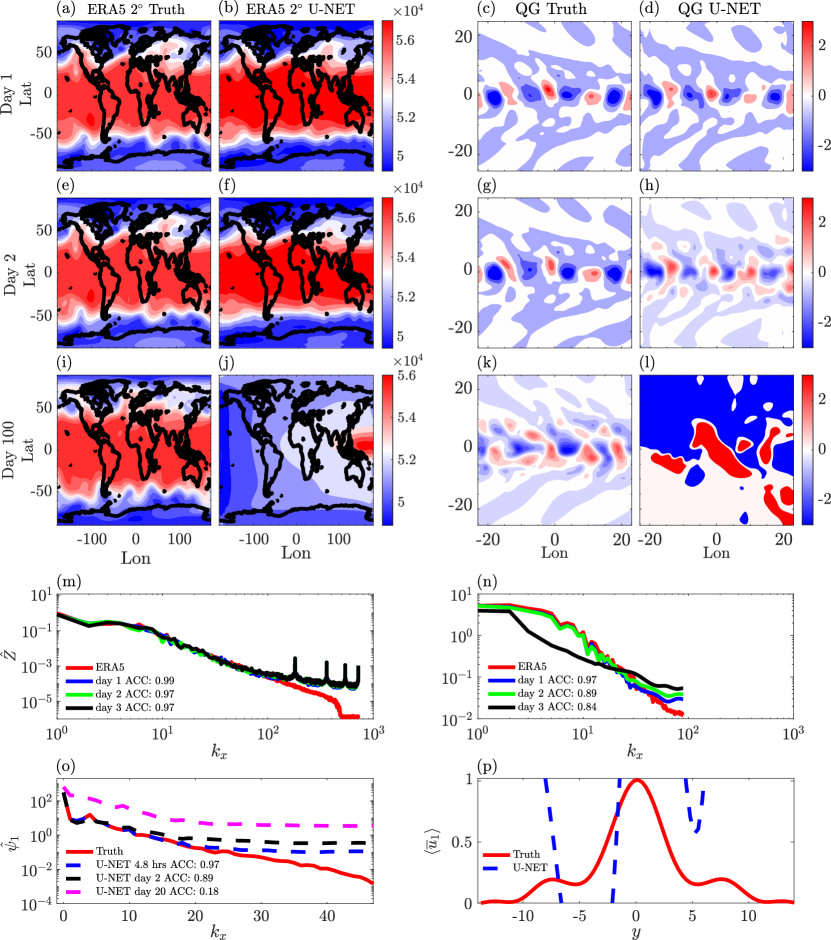
Figure 1: Long-term instabilities in a FourCastNet pathak2022fourcastnet and U-NET-based digital twin (section 4.3) trained on both $0.25^{\circ}$ and $2^{\circ}$ ERA5 data (section 4.1) and U-NET on QG simulations (section 4.2). (a) Z500 values from ERA5 on day 1 from year $2018$. (b) corresponding prediction of Z500 with U-NET. (c) True $\psi_{1}$ from numerical QG simulation at day 1. (d) Predicted $\psi_{1}$ from U-NET. (e) Z500 from day 2. (f) Day 2 prediction of Z500. (g) Prediction of $\psi_{1}$ but for day 2. (h) Similar to (d) but for day 2. (i) Z500 from ERA5 for day 100. (j) U-NET prediction of Z500 shows an unphysically diffused value. (k) $\psi_{1}$ at day 100 from QG simulation. (l) U-NET prediction shows unphysically large values near the jet. (m) FourCastNet’s prediction on $0.25^{\circ}$ ERA5 shows excellent prediction skill (ACC $\geq 0.99$) upto 3 days, but the latitude-averaged instantaneous Fourier spectrum of predicted Z500 fails to capture the small-scale part of the true spectrum beyond $k_{x}\geq 100$. (n) Similar to (m) but for U-NET on $2^{\circ}$ ERA5 showing a similar phenomenon. (o) Latitude-averaged instantaneous Fourier spectrum of predicted $\psi_{1}$ with U-NET shows that even for QG simulations, the small-scale part of the true spectrum cannot be captured right from the first time step of prediction ($4.8$ hrs). (p) $200-$ day autoregressive emulation with the U-NET trained on QG simulations, yield a physically inconsistent structure of the time- and zonal-mean upper-level velocity, $\left<\overline{u}_{1}\right>$. The Fourier spectrum demonstrated is averaged over predictions starting from $30$ initial conditions from separate ensembles.

We demonstrate spectral bias in deep learning architectures using FourCastNet pathak2022fourcastnet , a state-of-the-art model for data-driven weather prediction, and a baseline U-NET when trained on both ERA5 and QG data (more details on the data is given in section 4). In Fig. 1(a)-(l), we show that a U-NET-based digital twin trained on either $2^{\circ}$ ERA5 or QG data yields accurate short-term predictions but becomes unstable and shows unphysical values of $500$ hPa geopotential, Z500 (in case of ERA5) and upper- and lower-level stream function, $\psi_{1}$ and $\psi_{2}$ (in case of QG, where $1$ and $2$ are for the upper and lower level) after $100$ days of autoregressive emulation. Please note that a digital twin is not expected to predict the trajectory of the flow for a chaotic system after a short time period (typically 3-4 days in QG, and 5-7 days in ERA5). Hence, we have used the word emulation when referring to predictions at long time scales ($\approx 100$ days). The latitude-averaged absolute value of the zonal Fourier coefficients (zonal Fourier spectrum from now on) of the predictions, as shown in Fig. 1(m)-(o), reveal that FourCastNet trained on $0.25^{\circ}$ ERA5 data, U-NET trained on $2^{\circ}$ ERA5 data, and U-NET trained on QG data, fail to capture the small-scale part of the true Fourier spectrum of the fields (Z500 in case of ERA5 and $\psi_{1}$ in case of QG) during autoregressive prediction, starting from the first time step. For FourCastNet, the spikes in the Fourier spectrum occur due to the $8\times 8$ non-periodic patches used in the vision transformer, each of which passes through a fast Fourier transform inside Fourier neural operator (more details in Pathak et al. pathak2022fourcastnet ). The zonal Fourier spectrum has been computed since both the QG system and ERA5 have a jet moving along the zonal direction. The inability of the aforementioned deep neural networks to capture the small scales is attributed to the well-known theory of spectral bias xu2019frequency ; rahaman2019spectral ; basri2020frequency , an inductive bias that exists in all deep neural networks. This bias hinders the parameters of the networks to update, once the low-wavenumber components of the true signal’s Fourier spectrum is learned, thereby prohibiting the network to learn the high-wavenumber components. However, the common metrics used to determine the skill of the networks for forecasting tasks, such as ACC, do not get affected by the networks’ inability to capture the high-wavenumber part of the true spectrum and remain high (ACC $\geq 0.90$) even when the true and predicted spectrum does not match in the small scales.

The inability of the network to learn the small scales (high-wavenumber components of the true Fourier spectrum) manifests itself as an epistemic error. During the time of autoregressive prediction, the nonlinear interaction between the small and large scales cambon1999linear of the system, amplifies the errors in the predicted large-scale part of the true spectrum as well. Autoregressive emulation at long time scales ($\approx 100-200$ days) with such epistemic errors would finally result in an unphysical value of the emulated field. For example, in Fig. 1(p), we show the time- and zonal-mean structure of the emulated upper-level velocity, $\left<\overline{u}_{1}\right>$ (blue dashed line), in QG, which has no resemblance to the true time- and zonal-mean structure of $\left<\overline{u}_{1}\right>$. For QG, the model emulation shows spectral bias in predicted lower-level stream function, $\psi_{2}$, as well (Fig. S1(a)), which results in unphysically large values of the meridional heat flux during autoregressive emulation as shown in Fig. S1(b). This leads to an increase in the momentum flux as shown in Fig. S1(c), finally resulting in an unphysical value of lower-level velocity, $\left<\overline{u}_{2}\right>$ (Fig. S1(d)).

It must be highlighted here, that all deep neural networks, including fully-connected rahaman2019spectral , convolutional (this paper), operator (this paper), transformer-based (this paper), and generative schwarz2021frequency suffer from this epistemic error in the form of spectral bias, wherein they fail to learn the high-wavenumber components of the signal that they are trained to predict. This error is an inductive bias, which means that one cannot mitigate it by training on more data, longer epochs, or having more capacity in the network. However, in most classification problems involving natural images, capturing the low-wavenumber components of the signal is often enough to predict the probability of the correct class. For problems in multi-scale partial differential equations (PDEs) with tightly coupled spatiotemporal scales, such as in atmospheric, oceanic, and engineering turbulence, such epistemic errors along with their non-trivial and nonlinear propagation and subsequent amplification in the large scales would render all data-driven emulators useless.

Furthermore, one should note that while spectral bias is a universal and fundamental cause of instability, there may be other contributing causes as well, e.g., unphysical accumulation of kinetic energy near the poles (due to geometric distortion of data) in data-driven models of the atmosphere may lead to unphysical drifts as well. This has been addressed in Weyn et al. weyn2020improving through better geometric representations. Eliminating any of such many causes would not mitigate spectral bias. To elucidate that, we have also considered QG as an example where the distorting effect of poles is absent and yet the emulations become unstable due to spectral bias.

2.2 A solution: FouRKS (FOUrier-Runge-Kutta-with-Self-supervision)

In order to mitigate the instability arising due to spectral bias, we have adopted a principled approach to design FouRKS (shown in Fig 2), an architecture-agnostic framework, the details of which are described in section 4.4. FouRKS addresses spectral bias via a novel spectral regularizer (section 4.4.1 that penalizes the high wavenumbers during training, reduces error growth via a $4^{th}$-order Runge-Kutta (RK4) integrator implemented as a custom differentiable layer during training, and finally, a self-supervised spectrum-correction strategy to ensure that errors in the small scales are not allowed to propagate into the large scales during autoregressive prediction (inference stage). FouRKS can be used with any deep learning architecture, where the deep learning model is used to predict the residue of the underlying partial differential equation (PDE) of the system (more details in section 4.4).

2.2.1 Performance on QG

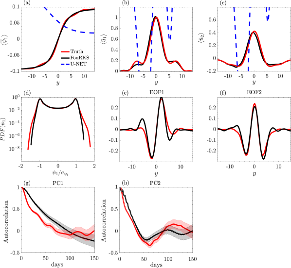
Figure 3: Long-term statistics showing the mean, PDF, and variability of predicted dynamics of QG using FouRKS (section 4.4) and baseline U-NET (section 4.3). The mean, PDF, and EOFs have been computed over $20000$ days of prediction. (a) Zonal- and time-mean upper-level stream function, $\left<\overline{\psi}_{1}\right>$, predicted by FouRKS (black solid line) shows excellent agreement with the true $\left<\overline{\psi}_{1}\right>$ (red solid line) obtained from the numerical QG simulation. Baseline U-NET (dashed blue line) shows large unphysical values for $\left<\overline{\psi}_{1}\right>$. (b) Zonal- and time-mean of upper-level velocity, $\left<\overline{u}_{1}\right>$, predicted by FouRKS and true $\left<\overline{u}_{1}\right>$ shows excellent agreement while U-NET’s predicted $\left<\overline{u}_{1}\right>$ is unphysical. (c) Same as (c), but for lower-level velocity, $\left<\overline{u}_{2}\right>$. (d) PDF computed with predicted $\psi_{1}$ with FouRKS shows agreement with the true PDF. PDF obtained from baseline U-NET could not be plotted with the same axis ranges owing to unphysically large values of the predicted fields. (e) EOF1 from FouRKS shows agreement with the true EOF1. EOF1 from baseline U-NET could not be computed since the predictions from U-NET are unphysically large after $20000$ days, making the numerical computation of EOFs infeasible. (f) Similar to (e) but for EOF2. (f) Autocorrelation of PC1 from FouRKS as compared to the autocorrelation of the true PC1. (g) Same as (f), but for the autocorrelation of PC2.

Applying FouRKS with a U-NET, on the QG system, we demonstrate stable long-term autoregressive emulation for $20000$ days for the first time. Figure 3 shows the long-term stable statistics obtained using the emulation from FouRKS after $20000$ days of autoregressive predictions on the QG system. Fig. 3(a)-(c) show that FouRKS has accurately captured the time- and zonal-mean structure of the upper-level stream function, $\psi_{1}$, and the upper- and lower-level velocities, $\left<\overline{u}_{1}\right>$, and $\left<\overline{u}_{2}\right>$ respectively. Fig. 3(d) shows that the PDF of $\psi_{1}$ (calculated over the region of the jetstream) is accurately captured by FouRKS as well. Figure 3(e)-(h) show that FouRKS can accurately predict the structure of the empirical orthogonal functions (EOFs) (also known as proper orthogonal modes, POD) as well as the principal component time series (PCs) which demonstrates its ability to capture the internal variability of the QG system.

2.2.2 Performance analysis of each component of FouRKS

Here, we investigate the effect of each component of FouRKS individually and together on short-term prediction skill and long-term stability.

In Fig. 4(a), the black solid line shows the root mean-squared error (RMSE) growth of the FouRK framework without the spectral regularizer (i.e., only the effect of RK4 integrator, as described in section 4.4.2 as a custom layer can be seen) as a function of time, during autoregressive prediction. As expected from a higher-order integrator, the RK4 layer dampens the growth of error as compared to the baseline U-NET (blue dashed line), for a longer period of time ($\approx$ 30 days). However, by $60$ days, the RMSE grows substantially and renders the predictions unphysical. Contrary to the RK4 layer, the spectral regularizer (section 4.4.1) pushes the RMSE error to grow faster than the regular U-NET (Fig. 4(b)). While it is not immediately clear as to why the spectral regularizer alone, has such an effect on the error growth in time, it must be kept in mind that, the regularizer only assists in capturing the small scales in a single time step of prediction. The effect of this regularizer on long-term autoregressive error propagation has not been studied and is not trivial owing to the absence of a theoretical framework for studying error propagation through neural network-based time integrators. Fig. 4(e) and (f) show the effect of the RK4 layer and the spectral regularizer on the Fourier spectrum of the predictions of $\psi_{1}$ (the effect on $\psi_{2}$ is similar, and not shown for brevity). While the higher-order integration scheme generally produces a more accurate state prediction whose Fourier spectrum better matches the true spectrum, it still cannot capture the smallest scales. However, the spectral regularizer alone can allow the network to produce predictions whose Fourier spectrum matches the true Fourier spectrum up to the smallest scales (blue solid line in Fig 4(f)) for a single time step. Combining RK4 and the spectral regularizer in FouRK allows the RMSE error to remain stable for $\approx 30$ days while marginally outperforming the baseline U-NET for short-term prediction ($3-5$ days) before eventually increasing to unphysically large values by $\approx 60$ days, as shown in Fig 4(c). This is because, despite the spectral regularizer diminishing spectral bias, and the RK4 integrator dampening error growth, the nature of the interaction of nonlinear scales in turbulence would amplify even the smallest of errors in the high wavenumbers and eventually render the emulation useless. The self-supervised spectrum-correction strategy in FouRKS, described in section 4.4.3 is thus, an essential component for long-term stability. FouRKS allows the RMSE error to remain bounded for long-term autoregressive predictions ($\approx$ 200 days), shown in Fig. 4(d). Moreover, with FouRKS, the Fourier spectrum of the predicted state matches all the scales of the true spectrum, even after $200$ days of prediction (Fig. 4(h)).

2.3 Performance on ERA5

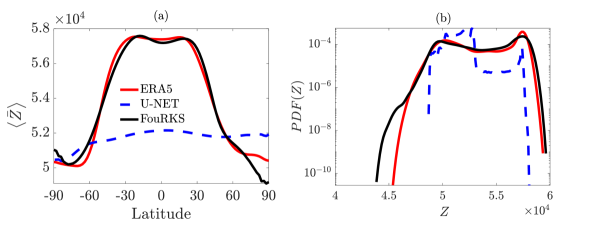
Figure 5: Long-term statistics of predicted Z500 with FouRKS calculated over $5200$ days of autoregressive prediction. (a) Zonal- and time-mean averaged Z500, $\left<\overline{Z}\right>$, predicted by FouRKS, U-NET as compared to ERA5. (b) PDF of Z500 computed from FouRKS’ prediction, U-NET’s prediction, and ERA5. Both the mean and PDF are accurately captured by FouRKS while U-NET shows unphysical predictions.

Here, for the first time, we show that FouRKS with a U-NET trained on $2^{\circ}$ Z500, Z50, and Z850 variables from ERA5 data can produce stable and physically consistent autoregressive predictions for up to 5200 days. As shown in Fig. 5(a), the time- and zonal-mean structure of the predicted Z500 matches that of ERA5 while the baseline U-NET shows an unphysical structure. A similar conclusion can be drawn from the structure of the PDF as well. We would like to point out that in this case, FouRKS was not able to get an accurate structure of EOF1 and EOF2 for Z500 and more analysis needs to be performed to understand why that is the case.

Figure 2: Schematics for each component of the FouRKS framework and the baseline U-NET. More details about each of the components can be found in section 4.3 and section 4.4.

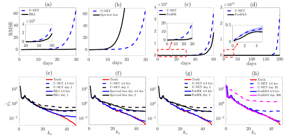
Figure 4: Growth of error in physical and spectral space during autoregressive prediction with different components in FouRKS (section 4.4). (a) Relative RMSE in FouRK without the spectral regularizer (black solid line) and baseline U-NET (blue dashed line) shows that the RK4 integrator diminishes the error growth during prediction as opposed to the baseline U-NET. It would however keep growing and become unphysical by $\approx 60$ days. (b) Relative RMSE in FouRK without the RK4 integrator, showing that the spectral regularizer does not diminish the error growth at all. (c) Relative RMSE in FouRK shows improvement in error growth as compared to baseline U-NET, but would still become unphysical by $\approx 60$ days. (d) Relative RMSE in FouRKS shows long-term stability as compared to baseline U-NET which becomes unphysical after $200$ days. (e) Fourier spectrum of predicted $\psi_{1}$ with FouRK ($\hat{\psi}_{1}$) without the spectral regularizer at the first time step of prediction ($4.8$ hrs) shown with solid blue line and day 1 (solid black line) as compared to U-NET (dashed lines). (f) Fourier spectrum of FouRK’s predicted $\psi_{1}$ without the RK4 integrator. The spectral regularizer alleviates spectral bias by capturing the full Fourier spectrum up to the smallest wavenumbers (solid blue line) as opposed to baseline U-NET. (g) Same as (f) but with FouRK having both the spectral regularizer and the RK4 integrator. (h) Fourier spectrum of predicted $\psi_{1}$ with FouRKS shows that the spectrum does not curl up during autoregressive prediction, even at $200$ days (solid magenta) as opposed to baseline U-NET whose predictions lose track of even the large scales (dashed magenta).

3 Discussion

In this paper, we report three major contributions to the field of data-driven digital twins for the climate system, and more broadly, multi-scale, dynamical systems such as turbulent flows:

(i) For the first time, we explain the cause of widely reported instabilities in deep learning-based digital twins of such systems and attribute it to spectral bias and subsequent error propagation during autoregressive predictions.

(ii) We propose FouRKS: an architecture-agnostic framework to mitigate spectral bias and perform convergent time integrations with the data-driven digital twins leading to dampened error propagation.

(iii) Finally, we demonstrate long-term stable and physically-consistent emulations with FouRKS for $20000$ days with data from a QG system and $5200$ days with ERA5 data.

This would facilitate accurate sub-seasonal to seasonal probabilistic weather forecasts, extreme weather forecasts, and replace expensive components of Earth system models with efficient data-driven emulators.

The spectral regularizer proposed in the FouRKS framework directly addresses the spectral bias issue during training. However, several other approaches to curbing spectral bias have been proposed in other studies as well that involve better design of activation functions, random feature kernels, etc rahaman2019spectral ; xu2019frequency ; hong2022activation ; li2019towards . Future work should focus on building architectural remedies to spectral bias as opposed to a soft constraint as in the case of our proposed spectral regularizer. It should also be kept in mind that for turbulent flow, the effect of spectral bias becomes much more prominent, especially during autoregressive prediction due to the multi-scale nature of turbulence. Hence, building effective mitigation strategies for spectral bias when building data-driven models for the climate system would require one to consider both turbulence physics and fundamental theoretical properties of deep neural networks at the same time.

The RK4 integrator in FouRKS dampens the error growth during prediction with the data-driven digital twin. Based on earlier work in Krishnapriyan et al krishnapriyan2022learning , the RK4 integrator is a convergent integration scheme for neural network-based integrators for dynamical systems. However, the fact that RK4-based integrators are convergent for deep neural networks, is still an empirical result. Future studies would benefit from developing rigorous theories, following in the footsteps of numerical analysis to understand a priori convergence properties of neural ordinary differential equations chen2018neural , and generally neural network-based integrators of dynamical systems.

The self-supervised spectrum-correction strategy is an intrusive step in FouRKS that increases the computational cost of autoregressive prediction. However, we have found in this study, that it is an essential component for obtaining accurate climate statistics. Several other studies stachenfeld2021learned ; wikner2022stabilizing , including ours chattopadhyay2022long , have found that training with noise, or training with variational models can improve the stability of autoregressive predictions. While there is an absence of rigorous theory to explain the effect of noise on stability, more focused studies need to be directed along these lines to better understand the effect of noise, during training, on autoregressive prediction. In this study, we conducted significant experimentation with different levels of white noise added to the labels during training. It did not improve the stability of the model.

While FouRKS allows the data-driven digital twin to produce long-term mean, PDF, and variability correctly, it is a long way away from being a fully functional climate model. Firstly, digital twins cannot generalize beyond the current climate, since it has been trained on the current climate and does not have a mechanism to account for radiative forcing. While one can easily fine-tune (transfer learn) digital twins on future simulations from state-of-the-art climate models, it would then suffer from the same numerical biases as that of climate models. Moreover, there are several other sanity checks that a climate model needs to pass before becoming operational. For example, a large body of literature analyses the responses of certain state variables predicted by climate models to small perturbations of certain other state variables hassanzadeh2016linear ; watson2022climatebench . These tests need to be meticulously performed and evaluated on data-driven digital twins for climate as well.

4 Data and Methods

4.1 Reanalyis data on two different resolutions

To evaluate the performance of the data-driven digital twins, we have considered two different resolutions of ECMWF reanalysis 5 (ERA5) data hersbach2020era5 . FourCastNet pathak2022fourcastnet is trained on $0.25^{\circ}$ resolution ERA5 and integrated with a time step of $\Delta t=6$h. FourCastNet uses a vision transformer combined with an adaptive Fourier neural operator in its architecture guibas2021efficient . Essential aspects on the training of FourCastNet can be found in Pathak et al. (pathak2022fourcastnet, ). The number of parameters in FourCastNet is $\approx 8\times 10^{6}$. The U-NET weyn2019can ; weyn2020improving ; chattopadhyay2021towards is trained on $2^{\circ}$ resolution ERA5 data and integrated with a time step of $\Delta t=1$ day. For the U-NET, training is performed on Z500, Z50, and Z850 data between $1979-2015$, validation is performed on the years of $2016$ and $2017$, and testing is performed by initializing the trained digital twin with $12$ independent initial conditions obtained from the year of $2018$.

4.2 The two-layer quasi-geostrophic (QG) system

The performance of the data-driven digital twins is also evaluated on the two-layer QG system. The QG system follows the set up as described in Philips phillips1951simple with a barocilinically unstable atmospheric jet. While the QG is not a comprehensive climate model, it is a reasonable representation of the essential aspects of the mid-latitude dynamics of the atmospheric jetstream and is an appropriate testcase for a fully turbulent flow. The full states of the system are given by the upper- and lower-level stream functions, $\psi_{1}$ and $\psi_{2}$. The equations solved in the two-layer QG system can be found in Lutsko et al. (lutsko2015applying, ) and Nabizadeh et al. (nabizadeh2019size, ).

For training on QG, we have used the full-state vectors, $\psi_{1}$ and $\psi_{2}$ from $8$ independent ensembles, each having $1500$ days of simulated flow. For validation, we have used another independent ensemble having $1500$ days of simulated flow. For testing, $30$ initial conditions from an independent ensemble have been used to intialize the trained digital twins. A time step, $\Delta t=40\Delta t_{n}$, has been used for training and autoregressive predictions, where $\Delta t_{n}$ is the time step used in the numerical simulation.

4.3 Baseline U-NET

Here, we describe how the U-NET, as shown in Fig 2, is trained to integrate the states of the system (both QG and ERA5) in time. The choice of U-NET is inspired from prior work in data-driven weather forecasting, where U-NET, and variants of U-NET, have been successfully used to predict atmospheric variables in short time scales (weyn2019can, ; weyn2020improving, ; weyn2021sub, ; chattopadhyay2021towards, ). The dynamics of both systems can be described as a PDE, with state vector, $\mathbf{X}$. The following mathematical treatment does not depend on whether we have access to the full states (as in QG) or partial states (as in ERA5) of the system. The evolution of the state, $\mathbf{X}$, is given by:

$$\frac{d\mathbf{X}}{dt}=\mathbf{F}\left(\mathbf{X}\left(t\right)\right).$$ (1)

The U-NET is trained on pairs of samples of $\mathbf{X}(t)$ and $\mathbf{X}(t+\Delta t)$. For QG, $\mathbf{X}$ consists of $\psi_{1}$ and $\psi_{2}$, while for the ERA5 data, it is Z500, Z50, and Z850. The objective of the U-NET, $\mathcal{M}\left[\circ,\phi\right]$, where $\phi$ are the trainable parameters, is to predict the right hand side of the equation:

$$\mathbf{X}(t+\Delta t)=\underbrace{\mathbf{X}(t)+\int_{t}^{t+\Delta t}{\mathbf{F}\left(\mathbf{X}\left(t\right)\right)}dt}_{\mathcal{M}\left[\mathbf{X}(t),\phi\right]}.$$ (2)

During inference, $\mathcal{M}$ is used to autoregressively predict the future states of the system, starting from an initial condition, $\mathbf{X}\left(t=0\right)$, obtained from an unseen test set.

The U-NET, $\mathcal{M}$, consists of $6$ hidden convolutional layers without pooling, an input layer, and an output layer. The first $4$ hidden layers have $64$ filters each. The second-last hidden layer has $128$ filters while the last hidden layer has $192$ filters. ReLU activations are used in the input and hidden layers, while the output layer has a linear activation function. A mean-squared error loss function is used. The loss is optimized using stochastic gradient descent with a fixed learning rate of $\alpha=10^{-9}$. The hyperparameters of the U-NET are been obtained after significant trial and error. $\mathcal{M}$ has $\approx 10^{5}$ trainable parameters.

4.4 FouRKS: FOUrier-Runge-Kutta-with-Self-supervision

In this paper, we propose an architecture-agnostic framework, FouRKS, which employs a three-pronged approach to mitigate instabilities and unphysical features in the data-driven digital twin’s predicted flow. The three prongs of FouRKS are:

• Fourier-based spectral regularization

• $4^{th}$-order Runge-Kutta integrator

• Self-supervised spectrum correction

The first two prongs are applied during training of the digital twin as shown in Fig 2 in the third row and the third prong is applied during autoregressive prediction with the digital twin as shown in Fig 2 in the fourth row.

4.4.1 Fourier-based spectral regularization

The first prong aims to penalize the high-wavenumber part of the latitude-averaged absolute value of zonal Fourier coefficients of the predicted fields so as to mitigate the effects of spectral bias. A spectral regularization term, $\mathbf{\mu}\left(\theta\right)$, is used in the loss function, given by :

$$\mathbf{\mu}\left(\theta\right)=\sum_{t=0}^{t=T}\biggr{\|}\widehat{\mathbf{X}}\left(t+\Delta t\right)\biggr{\rvert}_{{k_{x}\geq k_{T}}}-\widehat{\mathbf{H}}\left[\mathcal{N}\left(\mathbf{X}\left(t\right),\theta\right)\right]\biggr{\rvert}_{{k_{x}\geq k_{T}}}\biggr{\|}_{2}^{2},$$ (3)

such that the total loss function, $\mathbf{L}\left(\theta\right)$, is:

$$\mathbf{L}\left(\theta\right)=\sum_{t=0}^{t=T}\|\mathbf{X}\left(t+\Delta t\right)-\mathbf{H}\left[\mathcal{N}\left(\mathbf{X}\left(t\right),\theta\right)\right]\|_{2}^{2}+\lambda\mu(\theta),$$ (4)

where $\mathcal{N}$ is an U-NET that represents the right-hand-side of Eq.(1). More details on $\mathcal{N}$ is given in section 4.4.2. $\widehat{\left[\circ\right]}$ represents the absolute zonal Fourier coefficients averaged over all latitudes. However, we have found that, if we compute the latitude-averaged Fourier coefficients only over the midlatitudes for ERA5 and over the region of the jetstream in QG, the performance of FouRK or FouRKS is not affected. $T$ is the total number of temporal samples (across all the ensembles for QG and all the years for ERA5) that are used for training. $\lambda$ is the regularization constant (chosen as $0.8$ in this paper after significant trial and error). $k_{x}$ is the zonal wavenumber and $k_{T}$ (chosen as $30$ for QG and $40$ for ERA5 after significant trial and error) is the threshold wavenumber beyond which the absolute value of Fourier coefficients are penalized in $\mathbf{\mu}\left(\theta\right)$. Here, $\mathbf{H}\left[\circ\right]$ is a $4^{th}$-order Runge-Kutta (RK4) integrator implemented as a differentiable layer inside the architecture. Details on $\mathbf{H}$ is further explained in section 4.4.2.

4.4.2 A $4^{th}$-order Runge-Kutta (RK4) integrator

The second prong employs a RK4 time-integrator inside the architecture to dampen error propagation. Here, instead of directly predicting $\mathbf{X}(t+\Delta t)$, as done in Eq. (2), we represent $\mathbf{F}\left(\mathbf{X}\left(t\right)\right)$ in Eq. (1) with an U-NET, $\mathcal{N}\left[\circ,\theta\right]$, with trainable parameters, $\theta$:

$$\mathbf{X}(t+\Delta t)=\underbrace{\mathbf{X}(t)+\int_{t}^{t+\Delta t}\underbrace{\mathbf{F}\left(\mathbf{X}\left(t\right)\right)dt}_{\mathcal{N[\circ,\theta]}}}_{\mathbf{H[\circ]}}.$$ (5)

A custom layer, $\mathbf{H}[\circ]$, performs the integration between $t$ and $t+\Delta t$ via the RK4 scheme following Krishnapriyan et al. (krishnapriyan2022learning, ) as shown in Eq. (5). The operations in the $\mathbf{H}$ are given by:

$$i_{1} =\mathcal{N}\left[\mathbf{X}\left(t\right),\theta\right],$$ (6a)

$$i_{2} =\mathcal{N}\left[\mathbf{X}\left(t\right)+\frac{1}{2}i_{1},\theta\right],$$ (6b)

$$i_{3} =\mathcal{N}\left[\mathbf{X}\left(t\right)+\frac{1}{2}i_{2},\theta\right],$$ (6c)

$$i_{4} =\mathcal{N}\left[\mathbf{X}\left(t\right)+i_{3},\theta\right],$$ (6d)

$$z =\mathbf{X}\left(t\right)+\frac{1}{6}\left(i_{1}+2i_{2}+2i_{3}+i_{4}\right).$$ (6e)

The predicted state is given by $z=\mathbf{H}\left[\mathcal{N}\left(\mathbf{X}\left(t\right)\right),\theta\right]$. We denote any architecture equipped with the spectral regularizer and the RK4 integrator as FouRK. The number of parameters in the FouRK framework, where $\mathcal{N}\left[\circ,\theta\right]$ has the same architecture as described in section 4.3, is $\approx 10^{5}$. It should be noted that the choice of using $\mathbf{H}$ as an RK4 integrator is because it is convergent when used inside a neural network for integrating dynamical systems krishnapriyan2022learning . Other integrators with similar convergence properties can also be used.

4.4.3 Self-supervised spectrum correction

This third component is essential in the FouRKS framework to make FouRK stable for long-term climate simulations. FouRKS’ third prong is a self-supervised spectrum-correction strategy applied during autoregressive prediction. Here, at every $s$ days ($s=2$ in both QG and ERA5), FouRK updates its last two layers by implicitly optimizing a new loss function, $\mathbf{L}_{1}\left(\theta_{1}\right)$,

$$\mathbf{L_{1}}\left(\theta_{1}\right)=\biggr{\|}\left<\widehat{\mathbf{X}}_{train}\right>\biggr{\rvert}_{k_{x}\geq k_{T_{S}}}-\widehat{\mathbf{H}}\left[\mathcal{N}\left(\mathbf{X}\left(t\right),\theta\right)\right]\bigg{\rvert}_{k_{x}\geq k_{T_{S}}}\biggr{\|}_{2}^{2},$$ (7)

where $\theta_{1}$ are the parameters of the last two layers of $\mathcal{N}$ in FouRK. Here, $\left<\widehat{\mathbf{X}}_{train}\right>$ is the latitude-averaged zonal Fourier spectrum of the state, $\mathbf{X}$, averaged over the training set, where, $\left<\circ\right>$ denotes averaging over training set. $k_{T_{S}}$ is the threshold wavenumber chosen to be $20$ for QG and $30$ for ERA5 after several trials. Here the Fourier spectrum of $\mathbf{X}$ is invariant, i.e. in both the QG and ERA5 data, it does not change in time. This is because the QG system is stationary and while the true weather system is actually non-stationary, the variables that we are emulating (Z50, Z500, Z850) show a relatively constant structure of the Fourier spectrum over time. Thus, optimizing $\mathbf{L}_{1}\left(\theta_{1}\right)$ does not require any data. Here, $s$ and $k_{T_{S}}$ are hyperparameters which are obtained after extensive trial and error.

For this prong to be effective, another U-NET, $\mathcal{N}^{\prime}\left[\circ,\theta^{{}^{\prime}}\right]$, is trained to learn a map from $\widetilde{\mathbf{X}}(t)$ to $\mathbf{X}^{\prime}(t+\Delta t)$ as shown in Fig. 2, fourth row, where $\widetilde{\left[\circ\right]}$ is a sharp spectral filter with cut-off wavenumber as $k_{T_{S^{\prime}}}$ ($k_{T_{S^{\prime}}}=30$ for QG and $k_{T_{S^{\prime}}}=40$ for ERA5 after significant trial and error), and $\mathbf{X}^{\prime}=\mathbf{X}-\mathbf{\widetilde{X}}$. It uses the same loss function as in Eq. (4) during training, where $\mathbf{X}(t+\Delta t)$ is now replaced by $\mathbf{X}^{{}^{\prime}}(t+\Delta t)$. Similar to FouRK, this U-NET also undergoes a spectrum correction every $s$ daysduring autoregressive prediction with loss function, $\mathbf{L}_{2}\left(\theta^{{}^{\prime}}_{2}\right)$, given by:

$$\mathbf{L_{2}}\left(\theta^{{}^{\prime}}_{2}\right)=\biggr{\|}\left<\widehat{\mathbf{X^{\prime}}}_{train}\right>\biggr{\rvert}_{k_{x}\geq k_{T_{S^{\prime}}}}-\widehat{\mathcal{N^{\prime}}}\left(\mathbf{\widetilde{X}}\left(t\right),\theta^{{}^{\prime}}\right)\bigg{\rvert}_{k_{x}\geq k_{T_{S^{\prime}}}}\biggr{\|}_{2}^{2}.$$ (8)

$\theta^{{}^{\prime}}_{2}$ are the parameters of the last two layers of the U-NET, $\mathcal{N}^{\prime}$. The value of $k_{T_{S^{\prime}}}$ is a hyperparameter obtained through extensive trial and error. It should be carefully noted that $\mathcal{N^{\prime}}$ does not evolve a dynamical system. It is a map that learns to predict $\mathbf{X}^{\prime}$ from $\widetilde{\mathbf{X}}$, where $\widetilde{\mathbf{X}}$ is obtained by filtering the autoregressive prediction of $\mathbf{X}$ from FouRK. Hence, the burden of accurately predicting the state of the system lies on FouRK, while $\mathcal{N^{\prime}}$ is responsible for predicting the small scales, only one time step ahead.

At every $s$ days, the output from FouRK whose spectrum is corrected is filtered through a sharp spectral filter with cut-off wavenumber as $k_{T_{S^{\prime}}}$, and added to to the predicted $\mathbf{X}^{\prime}(t+\Delta t)$ as shown in Fig. 2, to obtain the modified state, $\mathbf{X}^{u}(t+\Delta t)$ at $t+\Delta t$:

$$\mathbf{X}^{u}(t+\Delta t)=\widetilde{\mathbf{X}}(t+\Delta t)+\mathbf{X}^{\prime}(t+\Delta t).$$ (9)

Acknowledgments

We thank Alistair Adcroft, Ebrahim Nabizadeh, Karthik Kashinath, Jaideep Pathak, and Laure Zanna for insightful comments and discussions. This work was supported by an award from the ONR Young Investigator Program (N00014-20-1-2722), a grant from the Schmidt Futures Program, and NASA grant 80NSSC17K0266 to P.H. Computational resources were provided by NSF XSEDE (allocation ATM170020) to use Bridges GPU and the Rice University Center for Research Computing. The codes for FouRKS are publicly available at https://github.com/ashesh6810/FouRKS.

References

- \bibcommenthead
- (1) Weyn, J.A., Durran, D.R., Caruana, R.: Improving data-driven global weather prediction using deep convolutional neural networks on a cubed sphere. Journal of Advances in Modeling Earth Systems 12(9), 2020–002109 (2020)
- (2) Rasp, S., Thuerey, N.: Data-driven medium-range weather prediction with a resnet pretrained on climate simulations: A new model for weatherbench. Journal of Advances in Modeling Earth Systems, 2020–002405 (2021)
- (3) Schultz, M., Betancourt, C., Gong, B., Kleinert, F., Langguth, M., Leufen, L., Mozaffari, A., Stadtler, S.: Can deep learning beat numerical weather prediction? Philosophical Transactions of the Royal Society A 379(2194), 20200097 (2021)
- (4) Weyn, J.A., Durran, D.R., Caruana, R., Cresswell-Clay, N.: Sub-seasonal forecasting with a large ensemble of deep-learning weather prediction models. Journal of Advances in Modeling Earth Systems 13(7), 2021–002502 (2021)
- (5) Chantry, M., Christensen, H., Dueben, P., Palmer, T.: Opportunities and challenges for machine learning in weather and climate modelling: hard, medium and soft ai. Philosophical Transactions of the Royal Society A 379(2194), 20200083 (2021)
- (6) Pathak, J., Subramanian, S., Harrington, P., Raja, S., Chattopadhyay, A., Mardani, M., Kurth, T., Hall, D., Li, Z., Azizzadenesheli, K., et al.: FourCastNet: A global data-driven high-resolution weather model using adaptive Fourier neural operators. arXiv preprint arXiv:2202.11214 (2022)
- (7) Bi, K., Xie, L., Zhang, H., Chen, X., Gu, X., Tian, Q.: Pangu-weather: A 3d high-resolution model for fast and accurate global weather forecast. arXiv preprint arXiv:2211.02556 (2022)
- (8) Lam, R., Sanchez-Gonzalez, A., Willson, M., Wirnsberger, P., Fortunato, M., Pritzel, A., Ravuri, S., Ewalds, T., Alet, F., Eaton-Rosen, Z., et al.: Graphcast: Learning skillful medium-range global weather forecasting. arXiv preprint arXiv:2212.12794 (2022)
- (9) Zeng, X., Li, Y., He, R.: Predictability of the loop current variation and eddy shedding process in the gulf of mexico using an artificial neural network approach. Journal of Atmospheric and Oceanic Technology 32(5), 1098–1111 (2015)
- (10) Andersson, T.R., Hosking, J.S., Pérez-Ortiz, M., Paige, B., Elliott, A., Russell, C., Law, S., Jones, D.C., Wilkinson, J., Phillips, T., et al.: Seasonal arctic sea ice forecasting with probabilistic deep learning. Nature communications 12(1), 1–12 (2021)
- (11) Reichstein, M., Camps-Valls, G., Stevens, B., Jung, M., Denzler, J., Carvalhais, N., et al.: Deep learning and process understanding for data-driven Earth system science. Nature 566(7743), 195–204 (2019)
- (12) Scher, S., Messori, G.: Weather and climate forecasting with neural networks: using general circulation models (gcms) with different complexity as a study ground. Geoscientific Model Development 12(7), 2797–2809 (2019)
- (13) Chattopadhyay, A., Mustafa, M., Hassanzadeh, P., Bach, E., Kashinath, K.: Towards physics-inspired data-driven weather forecasting: integrating data assimilation with a deep spatial-transformer-based U-NET in a case study with ERA5. Geoscientific Model Development 15(5), 2221–2237 (2022)
- (14) Keisler, R.: Forecasting global weather with graph neural networks. arXiv preprint arXiv:2202.07575 (2022)
- (15) Agarwal, N., Kondrashov, D., Dueben, P., Ryzhov, E., Berloff, P.: A comparison of data-driven approaches to build low-dimensional ocean models. Journal of Advances in Modeling Earth Systems 13(9), 2021–002537 (2021)
- (16) Mariotti, A., Ruti, P.M., Rixen, M.: Progress in subseasonal to seasonal prediction through a joint weather and climate community effort. npj Climate and Atmospheric Science 1(1), 1–4 (2018)
- (17) McKinnon, K.A., Rhines, A., Tingley, M., Huybers, P.: Long-lead predictions of eastern united states hot days from pacific sea surface temperatures. Nature Geoscience 9(5), 389–394 (2016)
- (18) Chattopadhyay, A., Nabizadeh, E., Hassanzadeh, P.: Analog forecasting of extreme-causing weather patterns using deep learning. Journal of Advances in Modeling Earth Systems 12(2), 2019–001958 (2020)
- (19) Stachenfeld, K., Fielding, D.B., Kochkov, D., Cranmer, M., Pfaff, T., Godwin, J., Cui, C., Ho, S., Battaglia, P., Sanchez-Gonzalez, A.: Learned simulators for turbulence. In: International Conference on Learning Representations (2022)
- (20) Su, J., Kempe, J., Fielding, D., Tsilivis, N., Cranmer, M., Ho, S.: Adversarial noise injection for learned turbulence simulations. Machine Learning for Physical Sciences Workshop, Advances in Neural Information Processing Systems (2022)
- (21) Li, Z., Kovachki, N., Azizzadenesheli, K., Liu, B., Bhattacharya, K., Stuart, A., Anandkumar, A.: Markov neural operators for learning chaotic systems. arXiv preprint arXiv:2106.06898 (2021)
- (22) Xu, Z.-Q.J., Zhang, Y., Luo, T., Xiao, Y., Ma, Z.: Frequency principle: Fourier analysis sheds light on deep neural networks. arXiv preprint arXiv:1901.06523 (2019)
- (23) Rahaman, N., Baratin, A., Arpit, D., Draxler, F., Lin, M., Hamprecht, F., Bengio, Y., Courville, A.: On the spectral bias of neural networks. In: International Conference on Machine Learning, pp. 5301–5310 (2019). PMLR
- (24) Basri, R., Galun, M., Geifman, A., Jacobs, D., Kasten, Y., Kritchman, S.: Frequency bias in neural networks for input of non-uniform density. In: International Conference on Machine Learning, pp. 685–694 (2020). PMLR
- (25) Cambon, C., Scott, J.F.: Linear and nonlinear models of anisotropic turbulence. Annual review of fluid mechanics 31(1), 1–53 (1999)
- (26) Schwarz, K., Liao, Y., Geiger, A.: On the frequency bias of generative models. Advances in Neural Information Processing Systems 34, 18126–18136 (2021)
- (27) Hong, Q., Tan, Q., Siegel, J.W., Xu, J.: On the activation function dependence of the spectral bias of neural networks. arXiv preprint arXiv:2208.04924 (2022)
- (28) Li, Z., Ton, J.-F., Oglic, D., Sejdinovic, D.: Towards a unified analysis of random fourier features. In: International Conference on Machine Learning, pp. 3905–3914 (2019). PMLR
- (29) Krishnapriyan, A.S., Queiruga, A.F., Erichson, N.B., Mahoney, M.W.: Learning continuous models for continuous physics. arXiv preprint arXiv:2202.08494 (2022)
- (30) Chen, R.T., Rubanova, Y., Bettencourt, J., Duvenaud, D.K.: Neural ordinary differential equations. Advances in neural information processing systems 31 (2018)
- (31) Stachenfeld, K., Fielding, D.B., Kochkov, D., Cranmer, M., Pfaff, T., Godwin, J., Cui, C., Ho, S., Battaglia, P., Sanchez-Gonzalez, A.: Learned coarse models for efficient turbulence simulation. arXiv preprint arXiv:2112.15275 (2021)
- (32) Wikner, A., Hunt, B.R., Harvey, J., Girvan, M., Ott, E.: Stabilizing machine learning prediction of dynamics: Noise and noise-inspired regularization. arXiv preprint arXiv:2211.05262 (2022)
- (33) Chattopadhyay, A., Pathak, J., Nabizadeh, E., Bhimji, W., Hassanzadeh, P.: Long-term stability and generalization of observationally-constrained stochastic data-driven models for geophysical turbulence. arXiv preprint arXiv:2205.04601 (2022)
- (34) Hassanzadeh, P., Kuang, Z.: The linear response function of an idealized atmosphere. part i: Construction using green’s functions and applications. Journal of the Atmospheric Sciences 73(9), 3423–3439 (2016)
- (35) Watson-Parris, D., Rao, Y., Olivié, D., Seland, Ø., Nowack, P., Camps-Valls, G., Stier, P., Bouabid, S., Dewey, M., Fons, E., et al.: Climatebench v1. 0: A benchmark for data-driven climate projections. Journal of Advances in Modeling Earth Systems 14(10), 2021–002954 (2022)
- (36) Hersbach, H., Bell, B., Berrisford, P., Hirahara, S., Horányi, A., Muñoz-Sabater, J., Nicolas, J., Peubey, C., Radu, R., Schepers, D., Simmons, A., Soci, C., Abdalla, S., Abellan, X., Balsamo, G., Bechtold, P., Biavati, G., Bidlot, J., Bonavita, M., Chiara, G.D., Dahlgren, P., Dee, D., Diamantakis, M., Dragani, R., Flemming, J., Forbes, R., Fuentes, M., Geer, A., Haimberger, L., Healy, S., Hogan, R.J., Hólm, E., Janisková, M., Keeley, S., Laloyaux, P., Lopez, P., Lupu, C., Radnoti, G., de Rosnay, P., Rozum, I., Vamborg, F., Villaume, S., Thépaut, J.-N.: The ERA5 global reanalysis. Quarterly Journal of the Royal Meteorological Society 146(730), 1999–2049 (2020)
- (37) Guibas, J., Mardani, M., Li, Z., Tao, A., Anandkumar, A., Catanzaro, B.: Efficient token mixing for transformers via adaptive fourier neural operators. In: International Conference on Learning Representations (2021)
- (38) Weyn, J.A., Durran, D.R., Caruana, R.: Can machines learn to predict weather? using deep learning to predict gridded 500-hpa geopotential height from historical weather data. Journal of Advances in Modeling Earth Systems 11(8), 2680–2693 (2019)
- (39) Phillips, N.A.: A simple three-dimensional model for the study of large-scale extratropical flow patterns. Journal of the Atmospheric Sciences 8(6), 381–394 (1951)
- (40) Lutsko, N.J., Held, I.M., Zurita-Gotor, P.: Applying the fluctuation–dissipation theorem to a two-layer model of quasigeostrophic turbulence. Journal of the Atmospheric Sciences 72(8), 3161–3177 (2015)
- (41) Nabizadeh, E., Hassanzadeh, P., Yang, D., Barnes, E.A.: Size of the atmospheric blocking events: Scaling law and response to climate change. Geophysical Research Letters 46(22), 13488–13499 (2019)