Study on Soft Robotic Pinniped Locomotion

Abstract

Legged locomotion is a highly promising but under–researched subfield within the field of soft robotics. The compliant limbs of soft-limbed robots offer numerous benefits, including the ability to regulate impacts, tolerate falls, and navigate through tight spaces. These robots have the potential to be used for various applications, such as search and rescue, inspection, surveillance, and more. The state-of-the-art still faces many challenges, including limited degrees of freedom, a lack of diversity in gait trajectories, insufficient limb dexterity, and limited payload capabilities. To address these challenges, we develop a modular soft-limbed robot that can mimic the locomotion of pinnipeds. By using a modular design approach, we aim to create a robot that has improved degrees of freedom, gait trajectory diversity, limb dexterity, and payload capabilities. We derive a complete floating-base kinematic model of the proposed robot and use it to generate and experimentally validate a variety of locomotion gaits. Results show that the proposed robot is capable of replicating these gaits effectively. We compare the locomotion trajectories under different gait parameters against our modeling results to demonstrate the validity of our proposed gait models.

I Introduction

Soft robots are manufactured with flexible materials (e.g., elastomers, fabrics, polymers, shape memory alloy) and are mostly actuated through pneumatic and hydraulic pressure, tendons, and smart materials [1]. Soft mobile robots – a branch of the soft robot family – use compliant structures (e.g., body, limbs, etc.) to achieve locomotion. They are mostly designed to mimic the behavior (typically locomotive patterns) of biological creatures [2]. Compared to rigid mobile robots, the inherently compliant elements in soft mobile robots enable them to absorb ground impact forces without active impedance control [3]. Furthermore, their ability to deform actively and passively allows them to gain access to confined areas [4]. As a result, soft mobile robots have great potential to replace humans in performing dangerous tasks, such as nuclear site inspection [5], search and rescue operations [6], and planetary exploration [7].

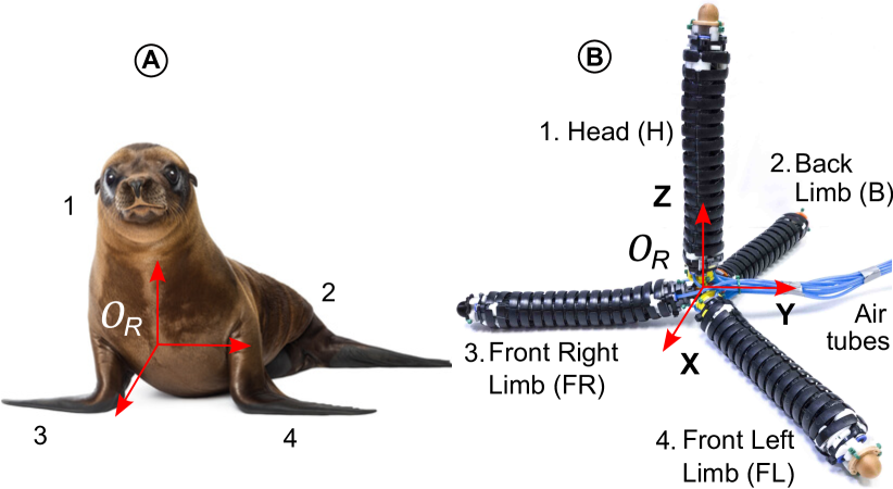
Figure 1: (A) Bioinspiration from pinnipeds (i.e., seals, sea lions, and walruses) that use fore flippers and body (or hind flipper) for terrestrial locomotion. (B) Pinniped robot in an unactuated pose.

Many soft-limbed robotic prototypes have been proposed to date [8]. For instance, the pneumatically actuated multi-gait robot reported in [9] uses five actuators to generate crawling and undulation gaits. However, it was only capable of preprogrammed straight locomotion without turning. The autonomous untethered quadruped in [10] is capable of carrying the subsystems (i.e., miniature air compressors, a battery, valves, and a controller). The robot can operate under adverse environmental conditions but only supports limited gaits. The quadruped in [11] can achieve various dynamic locomotion gaits such as crawling and trotting but without turning. The quadruped in [12] presents a new approach for controlling the gaits of soft-legged robots using simple pneumatic circuits without electronic components. The need for preprograming the gaits offer limited gait diversity. The soft robot prototypes reported in [13, 14] have stiffness-tunable limbs and are inspired by starfish, including its locomotion and water-vascular systems. But the low speed and low efficiency due to shape memory alloy actuators limit their utility. The amphibious soft robot in [15] uses highly compliant limbs with no stiffness tunability and resulting in unstable and slow locomotion. The soft-limbed hexapod proposed in [16] showed the ability to derive a variety of gaits. The hexapod appeared in [17] showed the ability to traverse challenging terrains. The large number of limbs however increases the robots’ complexity at the cost of limb dexterity. The soft-limbed robot proposed in [18] uses only four limbs in spatially symmetric tetrahedral topology. But due to the use of solenoid valves – binary actuation, it has limited control of the locomotion gaits. In addition, no analytical gait derivation approach was reported and only demonstrated preprogrammed locomotions.

We propose a new soft-limbed pinniped robot to address the above limitations. We adopt a modular design approach to increase the robustness and utilize hybrid soft limbs with improved payload and dexterous capabilities to fabricate the robot. In addition, we present a systematic approach to derive novel locomotion gaits. Further, we adopt a proportional limb bending mechanism to achieve improved workspace and control. The robot validates locomotion at a 38-fold speed increase than that of the state-of-the-art robot in [18]. Our main technical contributions are: i) designing and fabricating a novel pinniped robot using hybrid soft limbs; ii) deriving a complete floating-base kinematic model; iii) employing the kinematic model to derive fundamental limb movements; iv) parameterizing limb movements to derive new, sophisticated locomotion gaits; and v) experimentally validating the locomotion gaits under varying gait parameters.

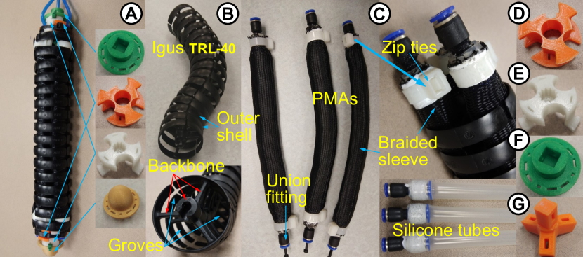
Figure 2: (A) Assembled soft limb. (B) Rigid kinematic chain. (C) PMAs. (D) Edge cap. (E) Middle joint. (F) Upper joint. (G) Tetrahedral joint.

II System Model

II-A Prototype Description

The proposed soft-limbed pinniped robot is shown in Fig. 1B. It consists of 4 identical soft limbs: Head (H), Back limb (B), Front Right limb (FR), and Front Left limb (FL). A soft limb (Fig. 2A) is actuated by three pneumatic muscle actuators (PMAs) and structurally supported by a backbone and outer shell (Fig. 2B). PMAs are fabricated using silicone tubes (Fig. 2C). PMAs are inserted into radially symmetric grooves (or channels) of the backbone structure (Figs. 2B and 2C) and further supported by 3D-printed parts shown in Figs. 2D, 2E, and 2F. We use Nylon threads to wrap PMAs in parallel to the backbone – in a way that the wrapping does not affect the bending performance – to prevent buckling upon extension during operation. This PMA and backbone arrangement results in an antagonistic actuator configuration since the backbone constrains the length change of PMAs during operation without constraining the omnidirectional bending. Further, the protective shell protects PMAs from potentially damaging environmental contacts. A soft limb has an effective length of $240~{}mm$, a diameter of $40~{}mm$, and a weight of $0.15~{}kg$. As shown in our previous work [19, 20, 21], this hybrid design (i.e., combining both soft and hard elements) increases the achievable stiffness range (hence payload) and provides decoupled stiffness and pose control.

We connect four soft limbs using a 3D-printed tetrahedral joint (Fig. 2G) to obtain the pinniped topology (Fig. 1). Thus, the robot has 12-DoF (3-DoF per limb) and weighs $0.65~{}kg$. In pinnipeds, the bulk of the mass is distributed toward the body (i.e., back end). However, we adopt this topology with symmetric mass distribution to optimize movements in all directions. Further, its spatial symmetry enables reorientation and thus better stability.

II-B Kinematics of Soft Limbs

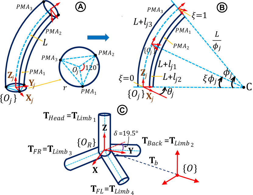
Figure 3: (A) Schematic of a soft limb design with actuator arrangement. (B) A view from an angle normal to the bending plane showing curve parameters. (C) Schematic of the pinniped robot.

Figures 3A and 3B show the schematic of a soft limb. Consider any j-th limb at a given time $t$. Let the length change of PMAs due to actuation be ${l_{ji}(t)}\in{\rm{\mathbb{R}}}$, for $i\in\{1,2,3\}$ and $j\in\{1,2,3,4\}$ where $i$ and $j$ stand for the PMA number and limb index, respectively. Thus, the joint variable vector of the j-th limb is expressed as $\textbf{{q}}_{j}=\left[{{l_{j1}},\,{l_{j2}},\,{l_{j3}}}\right]^{\mathsf{T}}$. The time dependency is omitted for brevity.

The body coordinate system of any j-th soft limb, $\{\boldsymbol{O_{j}}\}$, is defined at the geometric center of the cross-section on one end (termed base) with the first PMA – associated with $l_{j1}$ joint variable – anchor point coinciding with the $+X_{j}$ axis (Fig. 3A). The remaining PMAs with jointspace parameters $l_{j2}$ and $l_{j3}$ are indexed in counterclockwise direction at $\frac{2\pi}{3}$ angle offsets about $+Z_{j}$ from each other at $r_{j}$ distant from the origin of $\{\boldsymbol{O_{j}}\}$.

When PMAs are actuated with a resulting differential pressure, the torque imbalance at either end of the soft limb causes it to bend. As is the case with prior work on similarly-arranged soft robots, due to the uniform and symmetric construction, we can approximate that the limb’s neutral axis bends in a circular arc. Hence, the spatial pose of a soft limb can be parameterized by the angle subtended by the circular arc, $\phi_{j}$, and the angle to the bending plane w.r.t. the $+X_{j}$ axis, $\theta_{j}$. The radius of the circular arc can be derived as $\frac{L}{\phi_{j}}$ where $L\in\mathbb{R}$ is the unactuated length of a PMA (Fig. 3B). Using basic arc geometry [22], the curve parameters are derived using PMA lengths as

$$L+l_{ji} =\left\{\textstyle\frac{L}{\phi_{j}}-r\cos\left(\textstyle\frac{2\pi}{3}\left(i-1\right)-\theta_{j}\right)\right\}\phi_{j},\mbox{where}$$

$$l_{ji} =-r_{j}\phi_{j}\cos\left(\textstyle\frac{2\pi}{3}\left(i-1\right)-\theta_{j}\right).$$ (1)

Since the soft limb is inextensible, the sum of length changes of PMAs (i.e., jointspace variables) for all $i$ in (1) add up to zero. This results in the length constraint $l_{j1}=-\left(l_{j2}+l_{j3}\right)$, indicating that the complete limb kinematics can be expressed by two independent jointspace variables. From (1) and following [22, 23], we can derive the curve parameters (i.e., configuration space variables) in terms of the joint variables as

$$\phi_{j} =\textstyle\frac{2}{3r_{j}}\sqrt{\sum_{i=1}^{3}\textstyle\left(l_{ji}^{2}-l_{ji}\ l_{j\!\!\!\!\!\!\!\mod\left(i,3\right)+1}\right)},\ \mbox{and}$$ (2a)

$$\theta_{j} =\arctan\left\{\sqrt{3}\left(l_{j3}-l_{j2}\right),l_{j2}+l_{j3}-2l_{j1}\right\}.$$ (2b)

We derive the homogeneous transformation matrix (HTM) for any j-th soft limb, $\mathbf{T}_{j}\in\mathbb{SE}\left(3\right)$ as

$$\mathbf{T}_{j}\left(\boldsymbol{q},\xi\right) =\mathbf{R}_{Z}\left(\theta_{j}\right)\mathbf{P}_{X}\left(\textstyle\frac{L}{\phi_{j}}\right)\mathbf{R}_{Y}\left({\xi}\phi_{j}\right)\mathbf{P}_{X}\left(\textstyle-\frac{L}{\phi_{j}}\right)\mathbf{R}_{Z}\left(-\theta_{j}\right)$$

$$=\left[\begin{array}[]{cc}\mathbf{R}_{j}\left(\boldsymbol{q,{\xi}}\right)&\mathbf{p}_{j}\left(\boldsymbol{q,{\xi}}\right)\\ 0&1\end{array}\right],$$ (5)

where $\mathbf{R}_{Z}\in\mathbb{SO}\left(3\right)$ and $\mathbf{R}_{Y}\in\mathbb{SO}\left(3\right)$ define taskspace rotation matrices about $+Z_{j}$ and $+Y_{j}$, respectively, while $\mathbf{P}_{X}\!\in\mathbb{R}^{3}$ defines the taskspace translation matrix along $+X_{j}$. $\mathbf{R}_{j}\in\mathbb{SO}\left(3\right)$ and $\mathbf{p}_{j}\!\in\mathbb{R}^{3}$ give the homogeneous rotation and position matrices, respectively. The scalar $\xi\in[0,1]$ defines any point along the neutral axis of the limb (Fig. 3B). Refer to [22] for more information about the derivation.

II-C Inverse Kinematics of Soft Limbs

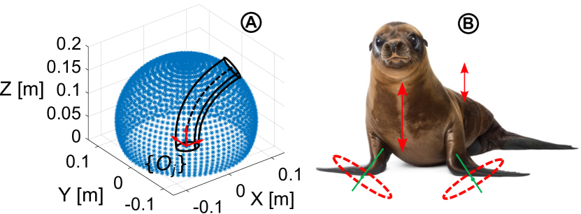
Figure 4: (A) Taskspace of a soft limb in its body coordinate frame, (B) Pinniped terrestrial crawling with limb, body, and head movements.

The relationship between the curve parameters and taskspace coordinates at the tip (i.e., $\xi=1$), $\mathbf{p}_{j}$ of (5), is given by

$$x_{j} =L\phi_{j}^{-1}\cos\left(\theta_{j}\right)\left\{1-\cos\left(\phi_{j}\right)\right\},$$ (6a)

$$y_{j} =L\phi_{j}^{-1}\sin\left(\theta_{j}\right)\left\{1-\cos\left(\phi_{j}\right)\right\},\ \mbox{and}$$ (6b)

$$z_{j} =L\phi_{j}^{-1}\sin\left(\phi_{j}\right),$$ (6c)

where $x_{j}$, $y_{j}$, and $z_{j}$ are the position vector elements w.r.t. the soft limb body coordinates frame, $\{\boldsymbol{O_{j}}\}$.

A soft limb taskspace – obtained from the kinematic model in (5) – is a symmetric shell about the $+Z_{j}$ axis of its body coordinate frame, as elucidated, $\{\boldsymbol{O_{j}}\}$, in Fig. 4A. Recall that, because of the length constraint imposed by the backbone (Sec. II-B), there are only two kinematic DoFs. Thus we can use two taskspace variables, $x_{j}$ and $y_{j}$, to derive the curve parameters $\theta_{j}$ and $\phi_{j}$. This can be done by solving for (7) that maps taskspace to curve parameters. Note that, there is no closed-form solution to (7). Thus, in this work, we utilize MATLAB’s ‘fmincon’ constrained optimization routine to solve it.

$$\theta_{j} =\arctan\left(y_{j},x_{j}\right),$$ (7a)

$$\phi_{j}^{-1}\left\{1-\cos\left(\phi_{j}\right)\right\} =L^{-1}\sqrt{x_{j}^{2}+y_{j}^{2}}.$$ (7b)

II-D Complete Robot Kinematics

Refer to the schematic of the robot shown in Fig. 3C. Utilizing (5), the HTMs of limbs, $\mathbf{T}_{Limb_{j}}\in\mathbb{SE}\left(3\right)$ relative to the robot coordinates frame, {$\boldsymbol{O}_{R}$}, located at the geometric center of the tetrahedral joint can be expressed as

$$\mathbf{T}_{Limb_{1}}\left({q{{}_{1}}},{\xi}\right) =\mathbf{T}_{1}\left({q_{1}},{\xi}\right),$$ (8a)

$$\mathbf{T}_{Limb_{2}}\left({q_{2}},{\xi}\right) =\mathbf{R}_{Y}\left({\textstyle\frac{\pi}{2}+\delta}\right)\mathbf{R}_{Z}\left({\textstyle{\pi}}\right)\mathbf{T}_{2}\left({q_{2}},{\xi}\right),$$ (8b)

$$\mathbf{T}_{Limb_{3}}\left({q_{3}},{\xi}\right) =\mathbf{R}_{Y}\left({\textstyle\frac{\pi}{2}+\delta}\right)\mathbf{R}_{Z}\left({\textstyle\frac{5\pi}{3}}\right)\mathbf{T}_{3}\left({q_{3}},{\xi}\right),$$ (8c)

$$\mathbf{T}_{Limb_{4}}\left({q_{4}},{\xi}\right) =\mathbf{R}_{Y}\left({\textstyle\frac{\pi}{2}+\delta}\right)\mathbf{R}_{Z}\left({\textstyle\frac{7\pi}{3}}\right)\mathbf{T}_{4}\left({q_{4}},{\xi}\right),$$ (8d)

where $\delta$ is $19.47^{\circ}$ (Fig. 3C) computed from the tetrahedral geometry. The complete kinematic model of the j-th limb of the robot can be obtained utilizing (8) with a floating-base coordinate frame, $\mathbf{T}_{b}\in\mathbb{SE}\left(3\right)$ as below.

$$\mathbf{T}_{Limb_{j}}\left({q}_{b},{q_{j}},{\xi}\right) =\mathbf{T}_{b}\left(q_{b}\right)\mathbf{T}_{Limb_{j}}\left({q_{j}},{\xi}\right),$$ (9)

$$\mathbf{T}_{b}(q_{b}) =\left[\begin{array}[]{cc}\mathbf{R}_{Z}\left({\alpha}\right)\mathbf{R}_{Y}\left({\beta}\right)\mathbf{R}_{X}\left({\gamma}\right)&\mathbf{p}_{b}\\ 0&1\end{array}\right].$$ (12)

Herein, ${q}_{b}=\left[x_{b},y_{b},z_{b},\alpha,\beta,\gamma\right]$ with $\left[\alpha,\beta,\gamma\right]$ and $\mathbf{p}_{b}=[x_{b},y_{b},z_{b}]^{\mathsf{T}}$ denote the orientation and translation variables of {$\boldsymbol{O}_{R}$} relative to the global coordinate frame {$\boldsymbol{O}$} (Fig. 3C).

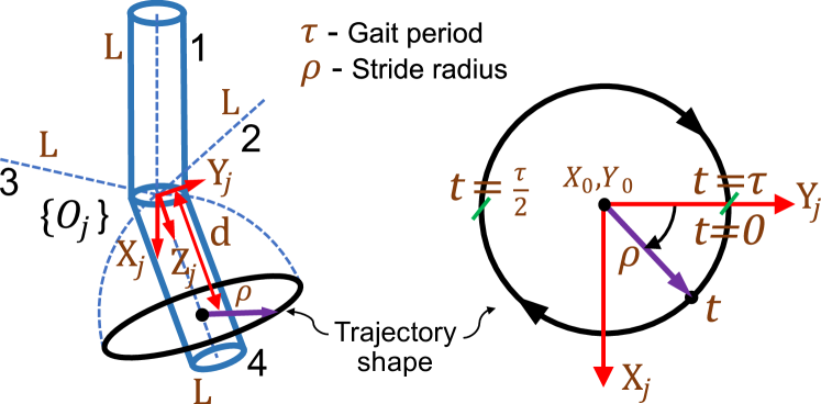
Figure 5: Fundamental motion trajectory of a soft limb.

III Locomotion Trajectory Generation

III-A Fundamental Limb Motion

The locomotion gaits derived here are inspired by the terrestrial crawling of pinnipeds (Fig. 4B). We use limb kinematics in Sec. II to parameterize and derive circular taskspace movement of the limb tip as the fundamental limb motion. For any j-th soft limb – shown in Fig. 5 – we define a circular trajectory of radius $\rho$ at $d$ distance from the limb’s origin, $\{O_{j}\}$, and period, $\tau$. At time $t$, the tip position relative to $\{O_{j}\}$ is given by

$${x_{j}=\rho\sin\left(\textstyle-\frac{2\pi t}{\tau}\right),\ y_{j}=\rho\cos\left(\textstyle-\frac{2\pi t}{\tau}\right),\ z_{j}=d}$$ (13)

We apply uniformly distributed $t\in\left[0,\tau\right]$ values on (13) to obtain a 100-point taskspace trajectory corresponding to the circular limb motion. We transform the taskspace trajectory to configuration space trajectory using the inverse kinematic model described in Sec. II-C. Subsequently, (1) is used to map the configuration space trajectory ($\theta_{j},\phi_{j}$) to the jointspace trajectory ($l_{ji}$).

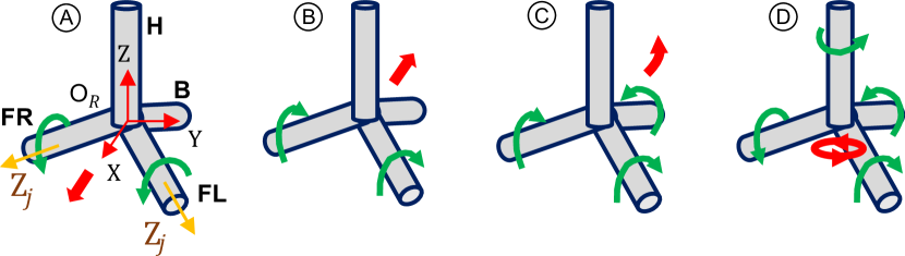
Figure 6: Limb trajectories: (A) Forward crawling, (B) Backward crawling, (C) Crawling-and-turning (Leftward), (D) In-place turning (counterclockwise).

III-B Effect of Center of Gravity

The center of gravity (CoG) of the robot helps stabilize locomotion [24]. We compute the robot CoG to investigate and regulate locomotion stability. From [25], the CoG of a limb, $\mathbf{c}_{j}\in\mathbb{R}^{3}$, relative to its body coordinate frame $O_{j}$} is

$$\mathbf{c}_{j}(q_{j})=\int_{0}^{1}\mathbf{p}_{j}(\xi,q_{j})d\xi.$$ (14)

Substituting $\mathbf{p}_{j}$ in (6) into (14), $\mathbf{c}_{j}(q_{j})$ can be derived as

$$\mathbf{c}_{j}(q_{j})=\frac{L}{\phi_{j}^{2}}\begin{bmatrix}\cos\left({\theta}_{j}\right)\left(\phi_{j}-\sin\left({\phi}_{j}\right)\right)\\ \sin\left({\theta}_{j}\right)\left(\phi_{j}-\sin\left({\phi}_{j}\right)\right)\\ \left(1-\cos\left({\phi}_{j}\right)\right)\end{bmatrix}.$$ (15)

Utilizing the results in (8) and (15), CoG relative to the robot coordinate frame, $\{O_{R}\}$, denoted by $\mathbf{C}_{j}\in\mathbb{R}^{3}$, can be obtained. If the mass of the j-th limb is $m_{j}$, then CoG of the robot relative to $\{O_{R}\}$, $\mathbf{C}_{R}\in\mathbb{R}^{3}$, can be written as

$$\mathbf{C}_{R}\left(q_{j}\right)=\frac{1}{\sum_{j=1}^{4}m_{j}}\sum_{j=1}^{4}m_{j}\mathbf{C}_{j}(q_{j}).$$ (16)

III-C Forward Crawling

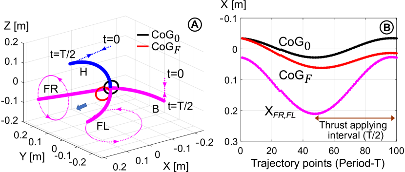
Figure 7: In forward crawling – (A) Spatial limb displacements and computed CoG trajectories, (B) CoG components and crawling limb tip displacements along the moving direction (i.e., $+X$ axis) relative to $O_{R}$.

We generate forward crawling locomotion by simultaneously (i.e., with zero phase offset) replicating the limb motion derived in Sec. III-A in FR and FL limbs as illustrated in Fig. 6A. Therein, we move the robot in $+X$ direction, by giving anticlockwise and clockwise motion trajectories to FR and FL limbs w.r.t. the local coordinate frames thereof, respectively. However, achieving forward crawling is challenging as there is, unlike pinnipeds with their relatively massive bodies, no body (or support limb) to counterbalance the angular moment generated by crawling forelimbs. Because of that, forward crawling in the proposed robot can induce instability.

We circumvent this limitation by controlling the CoG position given by (16) to obtain a more stable forward crawling gait as described below. Refer to Fig. 7A for the limb movements and CoG trajectories during a forward crawling cycle. We cyclically and proportionally bend the Head (H) limb towards the moving direction from a straight position ($\phi=0^{\circ}$) to a value computed using (16), $\phi=90^{\circ}$, during a locomotion cycle (Fig. 7A). This dynamic CoG control approach stabilizes the movement by counteracting instantaneous torque imbalances. We generate an additional thrust from the Back (B) limb (located on the opposite side) by actuating it in a manner that supports forward propelling. Therein, the B limb is gradually bent in a linear trajectory against the moving floor (Fig. 7A). As a consequence, the resultant limb displacement torque increases. Readers are referred to the experimental video on forward crawling to further understand the above limb actuating mechanism.

The impact of H and B limb actuation on crawling thrusts can be visualized by tracking the robot CoG and limb movements as shown in Figs. 7A and 7B. The CoG₀ denotes the CoG trajectory when H and B limbs are not actuated. When they are actuated, CoG₀ shifts towards the moving direction ($+X$) as noted by CoG_F in Fig. 7A. Figure 7B shows computed CoG₀, CoG_F, and crawling limb tips (X_FR, X_FL) in the moving direction relative to $O_{R}$. During the crawling thrust applying interval (i.e., ground contact period), the robot CoG converges and closely follows crawling limb tips as noted by CoG_F in Fig. 7B. It causes an increase in the weight-induced torque supported by the crawling limbs (FR & FL). As a consequence, with the increase in ground-limb reaction forces, the crawling thrusts increase.

III-D Backward Crawling

The backward crawling is referred to as moving in the $-X$ direction (Fig. 1B). Here, the limb motion derived in Sec. III-A is simultaneously applied to FR and FL limbs in the opposite direction to that of the forward crawling, i.e., FR and FL limbs are given clockwise and anticlockwise motion trajectories respectively, as illustrated in Fig. 6B. We keep the Head (H) limb bent in the $-X$ direction (i.e., backward) for shifting the robot CoG toward FR and FL limbs for improved stability and generating more thrust from the increased weight (reaction forces) at the limbs-ground contact [18]. Concurrently, the Back (B) limb is bent upward (in the $+Z$ direction of $O_{R}$) to reduce the contact surface and minimize the frictional resistance [18].

III-E Crawling-and-Turning

Pinnipeds use peristaltic body movement to propel forward since the bulk of the body weight is distributed towards the back (body) [26]. But, the proposed soft robot design has a symmetric weight distribution and thus it is difficult to maintain stability while propelling forward. As a consequence, the robot shows limited frontal movements. Conversely, when propelling backward, the torque imbalance is countered by the Body (i.e., B limb). It enables the use of the B limb in turning only in backward movements. Therefore, we opt to achieve turning in the backward direction. To achieve turning locomotion, we additionally actuate the B limb similarly to straight crawling limbs (FR & FL) discussed in Sec. III-C. For example, a clockwise trajectory of the B limb results in a leftward turn (Fig. 6C), while changing the direction of the B limb to anticlockwise results in a rightward turn. We replicate the B limb motion with different stride radii to control the turning effect. For example, a relatively large stride trajectory of the B limb can turn the robot efficiently (see results in Sec. IV and experimental videos).

III-F In-place Turning

In-place turning is referred to as the rotation about the robot $+Z$ axis (Fig. 1A). It is achieved by crawling all ground-contacting limbs in the same direction of rotation (clockwise/counterclockwise) as shown in Fig. 6D. Additionally, we actuate the Head (H) limb in the same direction of rotation in a circular trajectory at the same angular velocity. In that way, we shift the CoG of the Head (H) limb into the direction of rotation and support the turning. We can reverse the direction of in-place turning by reversing the direction of crawling in all limbs.

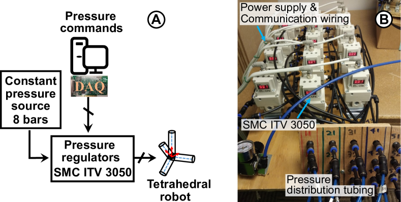
Figure 8: (A) Robot actuation setup, (B) Pressure regulator assembly.

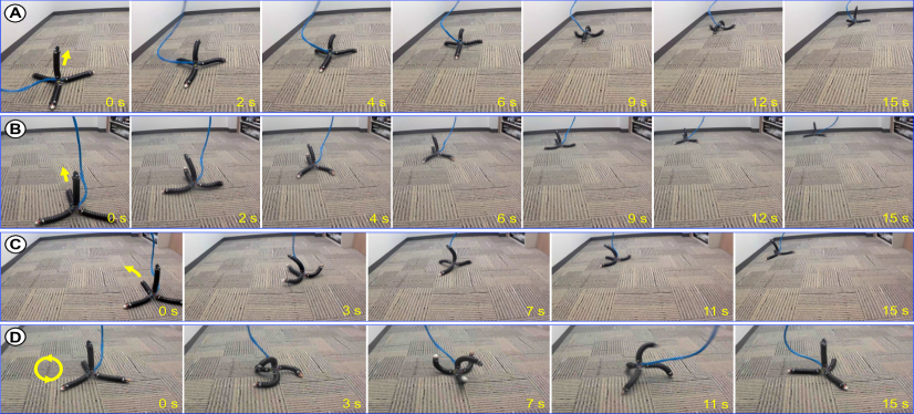
Figure 9: (A) Forward crawling, (B) Backward crawling, (C) Crawling-and-turning (leftward), (D) In-place turning (counterclockwise), at $0.10~{}m-1.00~{}Hz$.

IV Experimental Validation

IV-A Experimental Setup

The experimental setup for the robot is depicted in Fig. 8A. Air pressure is supplied from an $8-bar$ pneumatic source to digital proportional pressure regulators (ITV3050 31F3N3, SMC USA), as shown in Fig. 8B. The pressure regulators receive commands from a MATLAB Simulink Desktop Real-Time model through a data acquisition card (PCI-6703, NI USA), which sends an $0-10~{}V$ analog voltage signal. To make the soft limbs move and perform locomotion, the jointspace trajectories obtained in Sec. III must be converted into actuation pressure trajectories and input into the actuation setup shown in Fig. 8. The jointspace-pressure mapping reported in [27] is used to generate the corresponding pressure inputs. The robot is tested on a carpeted floor with approximately uniform friction, as seen in Fig. 9.

IV-B Testing Methodology

We actuated each gait for $15~{}s$ with a $3~{}bar$ actuator pressure ceiling (based on PMAs’ ability to achieve the required limb deformation). The frequency range, $\{0.75,1.00,1.25\}~{}Hz$ was chosen based on the operational bandwidth of PMAs to replicate meaningful locomotion. With 03 frequency combinations, we conducted 54 experiments for 06 straight crawling gaits, 06 crawling-and-turning gaits, and 06 in-place turning gaits as detailed in Secs. IV-C and IV-D.

IV-C Forward and Backward Crawling Gaits

We generated a total of 18 combinations of forward and backward crawling locomotion trajectories, with three gaits in each direction, using three different stride radii ($\rho_{1}=0.06~{}m$, $\rho_{2}=0.08~{}m$, $\rho_{3}=0.10~{}m$). Figures 9A and 9B show the progression of the robot during forward and backward crawling at the $0.10~{}m-1.00~{}Hz$ stride radius-frequency combination. Complete videos of the experiments are included in our multimedia submission. To determine the robot’s moving distance along the $X$ and $Y$ directions, we used the perspective image projection approach reported in [27, 28]. This approach utilized video feedback and floor carpet geometry data to estimate the distances. Note that some deviation from the intended gait is expected due to the performance variations of the custom-built PMAs powering the soft limbs.

We present the performance of each crawling gait in terms of estimated robot speed, which is shown in Table I. The experiments revealed that the robot achieved higher speeds at larger stride radii ($0.10~{}m$) and moderate actuation frequencies ($1.00~{}Hz$). This is because larger crawling strides generate stronger limb displacement torques on the floor than smaller strides. In addition, moderate actuation frequencies enable air pressure to reach the PMAs in a timely manner through the long pneumatic tubes, allowing for desired limb deformation without distortion of the torque amplitude. The highest recorded crawling speed was $16.9~{}cm/s$ ($0.65$ body length/second), which is a $38$-fold increase from the state-of-the-art reported in [18], $0.37cm/s$.

In forward crawling, the robot must perform additional limb deformations, as described in Sec. III-D, in order to maintain balance and generate additional forward propulsion. As a result, forward crawling recorded lower speeds compared to backward crawling at all times. The accompanying video further demonstrates that although forward crawling resembles pinniped locomotion, it is less efficient in maintaining forward locomotion stability.

TABLE I: Performance of Straight Crawling Gaits.

Straight Gait	Stride radius of crawling limbs (FR & FL)
	$\rho_{1}$ (0.06 $m$)			$\rho_{2}$ (0.08 $m$)			$\rho_{3}$ (0.10 $m$)
	Freq. [$Hz$]			Freq. [$Hz$]			Freq. [$Hz$]
	0.75	1.00	1.25	0.75	1.00	1.25	0.75	1.00	1.25
	Mean speed $[cm/s]$
Fwd Crawling	5.34	7.57	7.21	7.53	10.2	9.81	9.41	11.9	10.9
Bwd Crawling	7.21	10.1	9.83	9.52	13.5	13.0	11.9	16.9	16.1

TABLE II: Performance of Crawling-and-Turning gaits.

Turning Gait	Stride radius of turning limb (B limb)
	$\rho_{1}$ (0.04 $m$)			$\rho_{2}$ (0.06 $m$)			$\rho_{3}$ (0.08 $m$)
	Freq. [$Hz$]			Freq. [$Hz$]			Freq. [$Hz$]
	0.75	1.00	1.25	0.75	1.00	1.25	0.75	1.00	1.25
	Angular speed per unit distance $[rad/(ms)]$
Leftward Turn	1.13	1.72	1.70	1.59	2.24	2.06	2.22	2.89	2.41
Rightward Turn	1.15	1.68	1.65	1.62	2.31	2.11	2.35	2.92	2.49

IV-D Turning Gaits

We have successfully generated crawling-and-turning gaits for backward crawling locomotion (as described in Sec. III-E). We created 03 leftward and 03 rightward turning trajectories by varying the stride radius of the B limb at values of ($\rho_{1}=0.04~{}m$, $\rho_{2}=0.06~{}m$, $\rho_{3}=0.08~{}m$). For these gaits, the FR and FL limbs were actuated at a fixed stride radius of $0.10~{}m$.

TABLE III: Performance of In-place Turning gaits.

Turning Gait	Stride radius of crawling limbs (FR, FL, B)
	$\rho_{1}$ (0.06 $m$)			$\rho_{2}$ (0.08 $m$)			$\rho_{3}$ (0.10 $m$)
	Freq. [$Hz$]			Freq. [$Hz$]			Freq. [$Hz$]
	0.75	1.00	1.25	0.75	1.00	1.25	0.75	1.00	1.25
	Angular speed $[rad/s]$
Clockwise	2.75	3.29	3.09	3.01	3.55	3.41	3.35	3.76	3.51
Counterclockwise	2.81	3.35	3.12	3.08	3.69	3.53	3.42	3.82	3.59

For in-place turning, we produced six trajectories to represent clockwise/counterclockwise turning under three stride radii ($\rho_{1}=0.06~{}m$, $\rho_{2}=0.08~{}m$, $\rho_{3}=0.10~{}m$). During these gaits, all limbs, including the Head (H) limb, were actuated under the same stride radii as each crawling gait. Figures 9C and 9D show the leftward crawling-and-turning gait and counterclockwise in-place turning gait, respectively. The performance of these trajectories is presented in Tables II and III, respectively. We experimentally measured the turn angle and $X-Y$ floor displacement for all gaits using the method described in the straight crawling in Sec. IV-C. We then calculated the angular speed per unit distance for crawling-and-turning gait and the angular speed for in-place turning gait. According to the data in Table II, the effectiveness of turning increases with the stride radius of the turning limb. Similarly, the data in Table III indicates that the robot performs well in replicating in-place turning at higher stride radii, due to the increase in relative turn displacement torque with the applied trajectory stride radius.

V Conclusions

The soft-limbed robots have great potential for use in locomotion applications. We have designed a soft-limbed robot, which mimics pinniped locomotion, with a tetrahedral topology. The modular design approach for developing the robot was explained. Forward and inverse kinematic models for a single soft limb, as well as a complete floating-base kinematic model for the entire robot, were derived. The task-space trajectories for fundamental limb motion were proposed, and joint-space trajectories were obtained using kinematic models for forward/backward crawling, crawling-and-turning, and in-place turning gaits. The performance of the pinniped robot was experimentally validated under different stride radii and actuation frequencies, and the results show that the proposed locomotion trajectories were replicated well. Further work will focus on the development of dynamic gaits and closed-loop control of pinniped locomotion.

References

- [1] D. Rus and M. T. Tolley, “Design, fabrication and control of soft robots,” Nature, vol. 521, no. 7553, pp. 467–475, 2015.
- [2] F. Ahmed, M. Waqas, B. Javed, A. M. Soomro, S. Kumar, H. Ashraf, U. Khan, K. hwan Kim, and K. H. Choi, “Decade of bio-inspired soft robots: A review,” Smart Materials and Structures, 2022.
- [3] H. F. Al-Shuka, S. Leonhardt, W.-H. Zhu, R. Song, C. Ding, and Y. Li, “Active impedance control of bioinspired motion robotic manipulators: An overview,” Applied bionics and biomechanics, vol. 2018, 2018.
- [4] E. W. Hawkes, L. H. Blumenschein, J. D. Greer, and A. M. Okamura, “A soft robot that navigates its environment through growth,” Science Robotics, vol. 2, no. 8, p. eaan3028, 2017.
- [5] T. T. Oshiro, “Soft robotics in radiation environments: A prospective study of an emerging automated technology for existing nuclear applications,” 2018.
- [6] S. K. Talas, B. A. Baydere, T. Altinsoy, C. Tutcu, and E. Samur, “Design and development of a growing pneumatic soft robot,” Soft robotics, vol. 7, no. 4, pp. 521–533, 2020.
- [7] C. S. X. Ng and G. Z. Lum, “Untethered soft robots for future planetary explorations?” Advanced Intelligent Systems, p. 2100106, 2021.
- [8] Y. Sun, A. Abudula, H. Yang, S.-S. Chiang, Z. Wan, S. Ozel, R. Hall, E. Skorina, M. Luo, and C. D. Onal, “Soft mobile robots: a review of soft robotic locomotion modes,” Current Robotics Reports, pp. 1–27, 2021.
- [9] R. F. Shepherd, F. Ilievski, W. Choi, S. A. Morin, A. A. Stokes, A. D. Mazzeo, X. Chen, M. Wang, and G. M. Whitesides, “Multigait soft robot,” Proceedings of the national academy of sciences, vol. 108, no. 51, pp. 20 400–20 403, 2011.
- [10] M. T. Tolley, R. F. Shepherd, B. Mosadegh, K. C. Galloway, M. Wehner, M. Karpelson, R. J. Wood, and G. M. Whitesides, “A resilient, untethered soft robot,” Soft Robotics, vol. 1, no. 3, pp. 213–223, 2014.
- [11] I. S. Godage, T. Nanayakkara, and D. G. Caldwell, “Locomotion with continuum limbs,” in 2012 IEEE/RSJ International Conference on Intelligent Robots and Systems. IEEE, 2012, pp. 293–298.
- [12] D. Drotman, S. Jadhav, D. Sharp, C. Chan, and M. T. Tolley, “Electronics-free pneumatic circuits for controlling soft-legged robots,” Science Robotics, vol. 6, no. 51, 2021.
- [13] S. Mao, E. Dong, H. Jin, M. Xu, and K. Low, “Locomotion and gait analysis of multi-limb soft robots driven by smart actuators,” in 2016 IEEE/RSJ International Conference on Intelligent Robots and Systems (IROS). IEEE, 2016, pp. 2438–2443.
- [14] X. Huang, K. Kumar, M. K. Jawed, A. M. Nasab, Z. Ye, W. Shan, and C. Majidi, “Chasing biomimetic locomotion speeds: Creating untethered soft robots with shape memory alloy actuators,” Science Robotics, vol. 3, no. 25, p. eaau7557, 2018.
- [15] A. A. M. Faudzi, M. R. M. Razif, G. Endo, H. Nabae, and K. Suzumori, “Soft-amphibious robot using thin and soft mckibben actuator,” in 2017 IEEE International Conference on Advanced Intelligent Mechatronics (AIM). IEEE, 2017, pp. 981–986.
- [16] K. Suzumori, “Elastic materials producing compliant robots,” Robotics and Autonomous systems, vol. 18, no. 1-2, pp. 135–140, 1996.
- [17] Z. Liu, Z. Lu, and K. Karydis, “Sorx: A soft pneumatic hexapedal robot to traverse rough, steep, and unstable terrain,” in 2020 IEEE International Conference on Robotics and Automation (ICRA). IEEE, 2020, pp. 420–426.
- [18] Y. Wang, J. Wang, and Y. Fei, “Design and modeling of tetrahedral soft-legged robot for multi-gait locomotion,” IEEE/ASME Transactions on Mechatronics, 2021.
- [19] D. D. Arachchige and I. S. Godage, “Hybrid soft robots incorporating soft and stiff elements,” in 2022 IEEE 5th International Conference on Soft Robotics (RoboSoft). IEEE, 2022, pp. 267–272.
- [20] D. D. Arachchige, Y. Chen, I. D. Walker, and I. S. Godage, “A novel variable stiffness soft robotic gripper,” in 2021 IEEE 17th International Conference on Automation Science and Engineering (CASE). IEEE, 2021, pp. 2222–2227.
- [21] D. D. Arachchige, D. M. Perera, S. Mallikarachchi, I. Kanj, Y. Chen, and I. S. Godage, “Wheelless soft robotic snake locomotion: Study on sidewinding and helical rolling gaits,” in IEEE International Conference on Soft Robotics (RoboSoft), 2023, Accepted preprint: doi.org/10.48550/arXiv.2303.02285.
- [22] I. S. Godage, G. A. Medrano-Cerda, D. T. Branson, E. Guglielmino, and D. G. Caldwell, “Modal kinematics for multisection continuum arms,” Bioinspiration & biomimetics, vol. 10, no. 3, p. 035002, 2015.
- [23] B. A. Jones and I. D. Walker, “Kinematics for multisection continuum robots,” IEEE Transactions on Robotics, vol. 22, no. 1, pp. 43–55, 2006.
- [24] X. Wu, X. Shao, and W. Wang, “Stable quadruped walking with the adjustment of the center of gravity,” in 2013 IEEE International Conference on Mechatronics and Automation. IEEE, 2013, pp. 1123–1128.
- [25] I. S. Godage, R. Wirz, I. D. Walker, and R. J. Webster III, “Accurate and efficient dynamics for variable-length continuum arms: A center of gravity approach,” Soft Robotics, vol. 2, no. 3, pp. 96–106, 2015.
- [26] C. Kuhn and E. Frey, “Walking like caterpillars, flying like bats—pinniped locomotion,” Palaeobiodiversity and Palaeoenvironments, vol. 92, pp. 197–210, 2012.
- [27] D. D. Arachchige, Y. Chen, and I. S. Godage, “Soft robotic snake locomotion: Modeling and experimental assessment,” in 2021 IEEE 17th International Conference on Automation Science and Engineering (CASE). IEEE, 2021, pp. 805–810.
- [28] D. D. Arachchige, D. M. Perera, S. Mallikarachchi, I. Kanj, Y. Chen, H. B. Gilbert, and I. S. Godage, “Dynamic modeling and validation of soft robotic snake locomotion,” in IEEE International Conference on Control, Automation, and Robotics (ICCAR), 2023, Accepted preprint: doi.org/10.48550/arXiv.2303.02291.