Ton de Kok

Fixed non-stockout-probability policies for the single-item lost-sales model

Fixed non-stockout-probability policies for the single-item lost-sales model

Ton de Kok School of Industrial Engineering, Eindhoven University of Technology, P.O. Box 513, 5600MB Eindhoven, The Netherlands, a.g.d.kok@tue.nl

Abstract
We consider the classical discrete time lost-sales model under stationary continuous demand and linear holding and penalty costs and positive constant lead time. To date the optimal policy structure is only known implicitly by solving numerically the Bellman equations. In this paper we derive the first optimality equation for the lost-sales model. We propose a fixed non-stockout-probability ($FP_{3}$) policy, implying that each period the order size ensures that $P_{3}$, the probability of no-stockout at the end of the period of arrival of this order, equals some target value. The $FP_{3}$-policy can be computed efficiently and accurately from an exact recursive expression and two-moment fits to the emerging random variables. We use the lost-sales optimality equation to compute the optimal $FP_{3}$-policy. Comparison against the optimal policy for discrete demand suggests that the fixed $P_{3}$-policy is close-to-optimal. An extensive numerical experiment shows that the $FP_{3}$-policy outperforms other policies proposed in literature in $97\%$ of all cases. Under the $FP_{3}$-policy, the volatility of the replenishment process is much lower than the volatility of the demand process. This cv-reduction holds a promise for substantial cost reduction at upstream stages in the supply chain of the end-item under consideration, compared to the situation with backlogging.

Subject classifications
inventory/production: stochastic lost-sales model, review/lead times, optimality equation; probability: conditional random variables simulation: simulation-based optimization

lost-sales model, fixed non-stockout probability policy, conditional random variables, moment-iteration This paper was first submitted on April 8, 2023.

1 Introduction

We consider the classical periodic review single-item-single-echelon lost-sales model with constant integer lead times and linear holding and penalty costs. Over the last decade this model received considerable interest as new results have been derived regarding the optimal policy structure. We refer to Goldberg et al. (2016), Huh et al. (2009) for the asymptotic optimality of constant order ($CO$) policies for lead time to infinity, and the optimality of base stock ($BS$) policies for penalty costs to infinity, respectively. In this paper we propose a particular class of policies, which is inspired by van Donselaar et al. (1996), who show that a fixed fill rate policy outperforms the base stock policy. Instead of a fixed fill rate policy, we propose a fixed non-stockout probability policy, which is in line with the optimal policy under backlogging for the model under consideration. We denote this policy as $FP_{3}$ policy, the Fixed $P_{3}$ policy, using the notation in Silver et al. (2016), who denote the non-stockout probability as $P_{3}$. Through an extensive simulation study we show that this policy outperforms the BS policy, the CO policy, the capped base stock ($CBS$) policy proposed in Xin (2021), and the Projected Inventory Level ($PIL$) policy proposed in van Jaarsveld and Arts (2021). We also show that the costs of the $FP_{3}$-policy are remarkably close to the optimal costs for all cases in Zipkin (2008). Finding the optimal $FP_{3}$-policy is feasible by using the first explicit optimality equation for the lost-sales model, which is presented in this paper. We argue that we can always find a target $P_{3}$ value for which this optimality equation is satisfied. We use discrete event simulation combined with bisection to solve for the optimal $P_{3}$. An important auxiliary outcome of our experiments is that the $FP_{3}$-policy is not only cost-optimal, but also gives the lowest replenishment order coefficient of variation among all well-performing policies. This reverse bullwhip effect of the $FP_{3}$-policy should yield substantial cost reductions in the supply chain upstream of the stockpoint under consideration, compared with the situation where excess demand is backlogged. The paper is structured as follows. We introduce the model and its notation in section 2. The lost-sales optimality equation is presented in section 3. In section 4 we develop exact expressions for the targets of two myopic policies, the $FP_{3}$-policy and the $PIL$-policy, that must be met by the replenishment decision each period. We use the exact expressions to derive efficient and (in most cases) accurate approximations from which the replenishment quantity can be computed each period, taking into account the current inventory and all outstanding orders. An extensive numerical experiment in section 5 underpins the above statements concerning the performance of the $FP_{3}$-policy compared to other policies. We summarize our findings in section 6, where we also briefly discuss further research.

2 Model

We consider the periodic review lost-sales model, where at the start of each time unit an order is released, possibly of zero size. The lead time of an order is assumed to be constant and an integer number of time units. Inventory is replenished at the start of each time unit, before a new order is released. Demand in different time units is considered i.i.d. and assumed to be continuous. Demand not satisfied immediately from stock is lost. At the end of each time unit holding costs and penalty costs are incurred. Holding costs are incurred for each unit on stock at the end of the time unit. Penalty costs for each unit lost during the time unit are incurred at the end of the time unit. In Table 1 we provide the notation used throughout the paper. We use the convention that period $t$ starts at time $t-1$ and ends at time $t$. The objective of the paper is to analyze the cost performance of various policies proposed in literature and a policy we propose in this paper. We aim to minimize the long-run average cost, i.e. we do not consider a discount factor.

It is well-known that to-date the optimal policy for this lost-sales model is unknown and likely to be of a complicated structure. Below we show that a property of the optimal policy can be related to the first two moments of the stationary time between two stockouts. We argue that the same property holds for two heuristic policies. Stockout moments decouple to some extent the future evolution of the system from its past, but stockout moments are not regeneration points, as the state of the system, expressed by all individual outstanding orders, is a consequence of the past. Still, the evolution of the inventory during the intervals between stockout moments allows us to derive exact expressions for the cost difference between the optimal policy and a policy that follows from perturbation of the optimal policy.

In table 1 we present the notation used throughout the paper.

======== Insert table 1 about here ========

Below we omit the subscript $t$ when we consider the stationary version of the random variables defined above.

3 Optimal policy

The optimal policy for the lost-sales model is to-date unknown. In this section we derive a property of the optimal policy that is of use when determining optimal policies within classes of policies for the lost-sales model.

The long-run average costs $C$ can be written as

$$C=hE[\tilde{I}]+p(E[D]-E[Q]).$$

Without loss of generality we assume that at time 0 there is a stockout. Hence $T_{1}$ is the time of the first stockout after time 0. Then we can formulate the following theorem.

Theorem 1 Optimality equation for lost-sales systems
Under the optimal policy the following equation holds:

$$\frac{E[T^{2}]}{E[T]}={\frac{2p+h}{h}}\\$$ (1)

Proof of Theorem 1

We define the $n^{th}$ stockout moment $S_{n},n\geq 0$, as

$$S_{0}=0$$

$$S_{n}=\sum_{m=1}^{n}T_{m},n\geq 1.$$

Let us assume that the optimal policy yields optimal actions $\{Q^{*}_{t}\}_{t=1}^{\infty}$. We define an $\epsilon$-perturbed optimal policy by its actions,

$${\tilde{Q}_{t}(\epsilon)} =Q^{*}_{t}+\epsilon.$$

Note that this perturbation may imply that the optimal policy and the perturbed policy do not belong the the same class of policies. Define

$C^{*}$ := long-run average cost under the optimal policy

$C_{\epsilon}$ := long-run average cost under the $\epsilon$-perturbed policy

Let us consider the cost under both policies over the interval $(S_{n-1},S_{n}]$. As we let $\epsilon\to 0$, more and more stockout moments under the perturbed policy coincide with those under the optimal policy. In what follows, we ignore stockouts that do not coincide, knowing that in the limit for $\epsilon\to 0$, they represent zero probability mass. At time $S_{n-1}$ the inventory immediately after arrival of the replenishment order equals $Q^{*}_{S_{n-1}-L}$ under the optimal policy, and equals $Q^{*}_{S_{n-1}-L}+\epsilon$ under the $\epsilon$-perturbed optimal policy. Until time $S_{n}$ each order under the $\epsilon$-perturbed optimal policy adds another $\epsilon$ to the inventory in comparison to the optimal policy. At time $S_{n}$ a stockout occurs. Since we added $T_{n}$ times $\epsilon$ to the inventory under the optimal policy, the amount lost under the $\epsilon$-perturbed policy is $T_{n}\epsilon$ less than under the optimal policy. Thus, the cost difference over the interval $(S_{n-1},S_{n})$ between the two policies equals

$$\sum_{m=1}^{T_{n}-1}{h\epsilon m}-pT_{n}\epsilon=\epsilon(\frac{h}{2}T_{n}(T_{n}-1)-pT_{n}).\\$$

Then it follows that

$$C_{\epsilon}-C^{*} =\lim_{n\to\infty}\frac{\sum_{m=1}^{n}{\epsilon(\frac{h}{2}T_{n}(T_{n}-1)-pT_{n})}}{\sum_{m=1}^{n}T_{n}}$$

$$=\frac{\lim_{n\to\infty}\frac{1}{n}\sum_{m=1}^{n}{\epsilon(\frac{h}{2}T_{n}(T_{n}-1)-pT_{n})}}{\lim_{n\to\infty}\frac{1}{n}\sum_{m=1}^{n}T_{n}}$$

$$=\epsilon\frac{(\frac{h}{2}E[T(T-1)]-pE[T]}{E[T]}.$$

This implies that

$$\frac{C_{\epsilon}-C^{*}}{\epsilon}=\frac{h}{2}\frac{E[T^{2}]}{E[T]}-\frac{h}{2}-p.$$

As $C^{*}$ is the minimal cost under the optimal policy, we have

$$\lim_{\epsilon\to 0}\frac{C_{\epsilon}-C^{*}}{\epsilon}=0,$$

which implies that

$$\frac{h}{2}\frac{E[T^{2}]}{E[T]}=\frac{h}{2}+p,$$

This proves the theorem.

Note that $\frac{E[T^{2}]}{E[T]}$ is equal to the average time between the stockouts before and after some time $t$ for $t\to\infty$, if the times between stockouts would constitute a renewal process. It immediately follows from the optimality equation that $\frac{E[T^{2}]}{E[T]}$ is increasing in the penalty cost $p$. With increasing penalty cost, the non-stockout probability under the optimal policy increases. This suggests that $\frac{E[T^{2}]}{E[T]}$ is increasing in the non-stockout probability. A similar argument suggests that $\frac{E[T^{2}]}{E[T]}$ is increasing in the average inventory. Though we do not provide a formal proof of these statements, we have exploited them in our numerical experiments to find close-to optimal parameters for the fixed non-stockout probability ($FP_{3}$) policy. In the next section we discuss both $FP_{3}$-policy and $PIL$-policy in detail, deriving both exact expressions and computationally efficient approximations.

4 Myopic policies for the lost-sales problem

In van Donselaar et al. (1996) it is shown that for the lost-sales model, meeting a fill-rate constraint with a myopic policy that aims to meet this fill rate constraint every time unit is superior to meeting this fill rate constraint with a base stock policy. The myopic policy needs a lower average inventory and has a lower replenishment order volatility. For an inventory model with backordering and linear holding and penalty costs, de Kok (2018) shows that under mild conditions on the policy structure, the optimal policy within a class of policies satisfies the Newsvendor fractile, implying that the non-stockout probability at an arbitrary point in time must satisfy the Newsvendor fractile. For the periodic review backlog model without fixed costs and linear holding and penalty costs, the optimal policy is a myopic policy that aims to meet this Newsvendor fractile every period, which is in fact equivalent to a base stock policy. It should be noted that the cost structure for this classical backlog model is different from the cost structure for the lost-sales model in this paper. In the lost-sales model the penalty costs are linear in the number of items lost at the end of a period, whereas the penalty costs in the backlog model are linear in the number of items backlogged at the end of a period. While in the lost-sales model an item can incur penalty costs only once, in the backlog model the same item may be subject to a penalty cost over a number of periods. Still, the above discussion suggests that it should be worthwhile to study the cost performance of the myopic fixed non-stockout probability policy, where the replenishment order released ensures that at the moment of release, the non-stockout probability at the end of the period at the start of which this order replenishes inventory equals a fixed target value $P_{3}^{*}$.

4.1 Fixed non-stockout probability policy

The non-stockout probability at time $t+L+1$ can be written as

$$P_{3,t+L}=P\{(...((I_{t}-D_{t})^{+}+Q_{t-L+1}-D_{t+1})^{+}+...)+Q_{t}-D_{t+L}>0\}$$ (2)

This non-stockout probability is determined at time $t$, when ordering $Q_{t}$. Under the fixed non-stockout probability policy with target $P_{3}^{*}$, $\tilde{Q_{t}}$ is determined by

$$P\{(...((I_{t}-D_{t})^{+}+Q_{t-L+1}-D_{t+1})^{+}+...)+\tilde{Q_{t}}-D_{t+L}>0\}=P_{3}^{*}$$ (3)

It is easy to prove that, when starting with no outstanding orders and zero inventory, under continuous demand it is possible for all $t\geq 0$ to find $\tilde{Q_{t}}$ as a solution of equation (3). In van Donselaar et al. (1996) a numerical procedure is proposed to compute the fixed-fill-rate policy. This procedure can also be applied to solve equation (3). As it turns out, an alternative procedure can be applied to solve equation (3), along the same lines as proposed in de Kok (2003) for computing ruin probabilities. Firstly, this yields the following identities.

$$P_{3,t+L} =P\{(...((I_{t}-D_{t})^{+}+Q_{t-L+1}-D_{t+1})^{+}+...)+Q_{t}-D_{t+L}>0\}$$

$$=1-P\{((...((I_{t}-D_{t})^{+}+Q_{t-L+1}-D_{t+1})^{+}+...)+Q_{t}-D_{t+L})^{+}=0\}$$

$$=1-P\{D_{t+L}>Q_{t},D_{t+L+1}+D_{t+L}>Q_{t}+Q_{t-1},...,\sum_{s=0}^{L}D_{t+s}>I_{t}+\sum_{s=0}^{L-1}Q_{t-s}\}$$

Though the last equation shows that $P_{3,t+L}$ is determined by $L+1$ mutually dependent events, we can derive a set of recursive equations, introducing conditional random variables, that can be used for an efficient and accurate approximation of $P_{3,t+L}$. Towards that end we define,

$$\xi_{0} :=0$$

$$\xi_{n} :=\sum_{m=1}^{n}Q_{t+1-m},n=1,...,L$$

$$\xi_{L+1} :=I_{t}+\xi_{L}$$

$$X_{n} :=D_{t+L+1-n},n=1,...,L+1$$

Then it follows that

$$P_{3,t+L} =1-P\{\sum_{m=1}^{n}X_{m}>\xi_{n},n=1,...,L+1\}$$ (4)

With this we define the random variables $Y_{n},n=1,...,L+1$, to satisfy

$$P\{Y_{n}>x\}=\frac{P\{\sum_{k=1}^{m}X_{k}>\xi_{m},m=1,...,n-1,\sum_{k=1}^{n}X_{k}>x\}}{P\{\sum_{k=1}^{m}X_{k}>\xi_{m},m=1,...,n-1\}}$$ (5)

Note that

$$P\{Y_{1}>x\}=P\{X_{1}>x\}.$$

Similar as in de Kok (2003) we can derive from the above definition of $Y_{n},{n=1,...,L+1,}$ that

$$Y_{n}=X_{n}+(Y_{n-1}|Y_{n-1}>\xi_{n-1}),n=1,...,L+1,$$

which implies that

$$P\{Y_{n}>\xi_{n-1}\}=1,n=1,...,L+1.$$

We can define non-negative random variables $Z_{n},n=1,...,L+1$,

$$Z_{n}=Y_{n}-\xi_{n-1},n=1,...,L+1.$$ (6)

Then we find the following recursion for the conditional random variables $Z_{n},n=1,...,L+1$,

$$Z_{1} =X_{1},$$

$$Z_{n} =X_{n}+(Z_{n-1}-(\xi_{n-1}-\xi_{n-2}|Z_{n-1}>\xi_{n-1}-\xi_{n-2}),n=2,...,L+1.$$

This exact recursion is the basis for an efficient computation of an approximation of $P_{3,t+L}$. The recursion is based on the fact that $X_{n}$ is independent of $(Z_{n-1}-(\xi_{n-1}-\xi_{n-2}|Z_{n-1}>\xi_{n-1}-\xi_{n-2})$. This yields the following set of recursive equations,

$$E[Z_{1}] =E[X_{1}],$$

$$E[Z_{n}] =E[X_{n}]+E[(Z_{n-1}-(\xi_{n-1}-\xi_{n-2}|Z_{n-1}>\xi_{n-1}-\xi_{n-2})],n=2,...,L+1.$$

$$\sigma^{2}(Z_{1}) =\sigma^{2}(X_{1}),$$

$$\sigma^{2}(Z_{n}) =\sigma^{2}(X_{n})+\sigma^{2}((Z_{n-1}-(\xi_{n-1}-\xi_{n-2}|Z_{n-1}>\xi_{n-1}-\xi_{n-2})),n=2,...,L+1.$$

The first two moments of $(Z_{n-1}-(\xi_{n-1}-\xi_{n-2})|Z_{n-1}>\xi_{n-1}-\xi_{n-2})$ are easy to compute for probability distributions such as gamma, mixed Erlang, and shifted exponential (cf. Tijms (2003)). Thus, we can find expressions for the first two moments of $Z_{n},n=1,...,L+1$, and fit a distribution on these moments to obtain an approximation for $P\{Z_{n}>\xi_{n}-\xi_{n-1}\},n=1,...,L+1$. It follows from equations (4), (5), and (6) that

$$P_{3,t+L} =1-\prod_{n=1}^{L+1}P\{Z_{n}>\xi_{n}-\xi_{n-1}\}$$ (7)

Equation (7) gives an exact expression for the non-stockout probability $P_{3,t+L}$. Together with the approximations for $P\{Z_{n}>\xi_{n}-\xi_{n-1}\},n=1,...,L+1$, from the two-moment recursion scheme, we find an approximation for $P_{3,t+L}$. In section 5 we show that this approximation is remarkably accurate when assuming demand per period is mixed Erlang distributed and fitting mixed Erlang distributions on the first two moments of $Z_{n},n=1,...,L+1.$

At every time $t$, the fixed non-stockout probability ($FP_{3}$) policy, solves $Q_{t}$ from equation (7) with $P_{3,t+L}=P_{3}^{*}$. As $Q_{t}=\xi_{1}$ we choose some initial value of $Q_{t}$, subsequently apply the moment-iteration scheme to compute $P_{3,t+L}$ from equation (7), and compare $P_{3,t+L}$ and $P_{3}^{*}$. Thus, a bisection scheme yields $Q_{t}$.

We note here that the moment iteration scheme proposed in van Donselaar et al. (1996) could be applied here, too. But we found that this scheme, though more efficient in computing $Q_{t}$, yields less accurate results. As we wanted to compare the performance of the $FP_{3}$ policy against asymptotically optimal policies, we needed a very accurate approximation scheme.

Furthermore, we stipulate that, when applying the $FP_{3}$ policy in practice, we need to calculate only a single $Q_{t}$ each period for each sku. With current computational power, this is a matter of seconds for thousands of sku’s.

4.2 Asymptotic behaviour of the $FP_{3}$-policy

In the next section we show the accuracy of the approximation for $P_{3,t+L}$ and discuss the performance of the $FP_{3}$ policy against that of asymptotically optimal policies. In this subsection we discuss the asymptotic behaviour of the $FP_{3}$-policy for high target values of $P_{3,t+L}$ and long lead times. Let us first consider the situation of high target values of $P_{3,t+L}$. In order to maintain such high service levels, we need to maintain high levels of $I_{t}$. We can see the implication of high levels of $I_{t}$ on the decision variable $Q_{t}$ by rewriting equation 4 as follows,

$$P_{3,t+L} =1-P\{\sum_{m=1}^{n}X_{m}>\xi_{n},n=1,...,L+1\}$$

$$=P\{\cup_{n=1}^{L+1}\{\sum_{m=1}^{n}X_{m}\leq\xi_{n}\}\}$$

$$=P\{X_{L+1}\leq\xi_{L+1}\}+P\{X_{L+1}>\xi_{L+1},\cup_{n=1}^{L}\{\sum_{m=1}^{n}X_{m}\leq\xi_{n}\}\}$$

As the penalty cost $p\to\infty$, $P_{3}^{*}\to 1$ and thereby $I_{t}\to\infty$. This implies that $\xi_{L+1}\to\infty$. Then it follows that

$$\lim_{p\to\infty}\frac{P_{3,t+L}}{P\{X_{L+1}\leq\xi_{L+1}\}}=1$$

Hence for large values of $p$ we can solve for $Q_{t}$ by solving

$${P\{\sum_{n=0}^{L}D_{t+s}\leq I_{t}+\sum_{n=0}^{L-1}Q_{t-s}\}}=P_{3}^{*}$$

But solving this equation is equivalent to operating under a base stock policy. Thus for high penalty costs the $FP3$-policy behaves like a base stock policy.

Now let us consider the case for $L\to\infty$. Assuming that under the $FP_{3}$-policy the system eventually reaches stationarity, the order quantity $Q_{t}$ arrives after an infinite amount of time and therefore finds the inventory in its stationary state $I$. Thus $Q_{t}$ follows from the following equation,

$$P\{I+Q_{t}-D\}=P_{3}^{*}$$

Then it follows that every $Q_{t}$ satisfies the same equation and thus for $L\to\infty$, the $FP_{3}$-policy behaves as a constant order policy. Thus the $FP_{3}$-policy is optimal under the asymptotic regimes studied in Huh et al. (2009) and Goldberg et al. (2016).

4.3 Projected inventory level policy

A myopic policy related to the fixed-fill-rate and fixed-non-stockout-probability policies is the fixed projected-inventory-level ($PIL$) policy proposed by van Jaarsveld and Arts (2021). Under this policy, each period the replenishment order quantity is determined such that a target expected inventory at the start of the period, immediately after the order is added to inventory, is met. It is shown in van Jaarsveld and Arts (2021) that the $PIL$ policy is asymptotically optimal for long lead times and high penalty costs. In section 6 we compare the $FP_{3}$ policy with the $PIL$ policy. For that purpose we develop an exact expression for the expected inventory $E[\tilde{I}_{t+L-1}]$. Note that

$$\tilde{I}_{t+L-1}:=(I_{t+L-1}-D_{t+L-1})^{+}.\\$$

Then it follows that

$$I_{t+L}=\tilde{I}_{t+L-1}+Q_{t}.\\$$

Basic probability theory yields

$$E[\tilde{I}_{t+L-1}]:=\int_{0}^{\infty}(1-P\{\tilde{I}_{t+L-1}\leq x\})dx.$$ (8)

Similar to the derivation of the expression for $P_{3,t+L}$, we find an expression for $P\{\tilde{I}_{t+L-1}\leq x\}$,

$$P\{\tilde{I}_{t+L-1}\leq x\} =P\{(...((I_{t}-D_{t})^{+}+Q_{t-L+1}-D_{t+1})^{+}+...)+Q_{t-1}-D_{t+L-1})^{+}\leq x\}$$

$$=P\{(...((I_{t}-D_{t})^{+}+Q_{t-L+1}-D_{t+1})^{+}+...)+Q_{t-1}-x-D_{t+L-1})^{+}=0\}$$

We define $\tilde{X}_{n}$ and $\tilde{\xi}_{n},n=1,...,L$,

$$\tilde{\xi}_{0} :=0$$

$$\tilde{\xi}_{n} :=\sum_{m=1}^{n}Q_{t-m},n=1,...,L-1$$

$$\tilde{\xi}_{L} :=I_{t}+\tilde{\xi}_{L-1}$$

$$\tilde{X}_{n} :=D_{t+L-n},n=1,...,L$$

Similar to the derivation of equation 4 we find

$$P\{\tilde{I}_{t+L-1}\leq x\}=P\{\sum_{m=1}^{n}\tilde{X}_{m}\geq\tilde{\xi}_{n}-x,n=1,...,L\}.\\$$

Substitution of this equation into equation (8) and using $\tilde{\xi}_{0}=0$ yields

$$E[\tilde{I}_{t+L-1}] =\int_{0}^{\infty}(1-P\{\sum_{m=1}^{n}\tilde{X}_{m}\geq\tilde{\xi}_{n}-x,n=1,...,L\})dx$$

$$=\sum_{k=1}^{L}{\int_{\tilde{\xi}_{k-1}}^{\tilde{\xi}_{k}}(1-P\{\sum_{m=1}^{n}\tilde{X}_{m}\geq\tilde{\xi}_{n}-x,n=1,...,L\})dx}.$$

As $\tilde{\xi}_{1}\leq\tilde{\xi_{2}}\leq...\leq\tilde{\xi}_{L}$, we find that

$$\tilde{\xi}_{n}-x\leq 0,n=0,...,k-1,x\in(\tilde{\xi}_{k-1},\tilde{\xi}_{k}),k=1,...,L.$$

With this we can write $E[\tilde{I}_{t+L-1}]$ as

$$E[\tilde{I}_{t+L-1}] =\sum_{k=1}^{L}{\int_{\tilde{\xi}_{k-1}}^{\tilde{\xi}_{k}}(1-P\{x+\sum_{m=1}^{n}\tilde{X}_{m}\geq\tilde{\xi}_{n},n=k,...,L\})dx}.$$

Introducing the uniformly distributed random variables $W_{k},\\ k=1,...,L$,

$$W_{k}\overset{d}{=}U(0,\tilde{\xi}_{k}-\tilde{\xi}_{k-1}),\\$$

we find the following expression for $E[\tilde{I}_{t+L-1}]$,

$$E[\tilde{I}_{t+L-1}] =\sum_{k=1}^{L}{(\tilde{\xi}_{k-1}}-{\tilde{\xi}_{k}})(1-P\{W_{k}+\sum_{m=1}^{n}\tilde{X}_{m}\geq\tilde{\xi}_{n}-\tilde{\xi}_{k-1},n=k,...,L\}).$$

This equation can be rewritten with the help of the following (random) variables for $k=1,...,L$,

$$\hat{X}_{k1} =W_{k}+\sum_{m=1}^{k}\tilde{X}_{m}$$

$$\hat{X}_{kn} =\tilde{X}_{k+n-1},n=2,...L+1-k$$

$$\hat{\xi}_{kn} =\tilde{\xi}_{k+n-1}-\tilde{\xi}_{k-1},n=1,...,L+1-k.$$

Thus, we find an exact expression for $E[\tilde{I}_{t+L-1}]$,

$$E[\tilde{I}_{t+L-1}] =\sum_{k=1}^{L}{(\tilde{\xi}_{k-1}}-{\tilde{\xi}_{k}})(1-P\{\sum_{m=1}^{n}\hat{X}_{km}\geq\hat{\xi}_{kn},n=1,...,L+1-k\}).$$ (9)

Note that the probabilistic expressions on the right-hand side of equation (9) are identical to the expression for $P_{3,t+L}$ in equation (4). We can reuse our approximation scheme based on fitting mixtures of Erlang distributions to compute an approximation for $E[\tilde{I}_{t+L-1}]$. Using this scheme, it follows that computation of the approximation for $E[\tilde{I}_{t+L}]$ requires a factor of $\frac{L}{2}$ more CPU time.

This concludes this section in which we developed exact expressions for $P_{3,t+L}$ and $E[\tilde{I}_{t+L}]$. The exact expression for $P_{3,t+L}$ can be translated into an exact recursive scheme for computational purposes. This recursive scheme is used as the basis for efficient approximations for $P_{3,t+L}$ and $E[\tilde{I}_{t+L}]$ using mixtures of Erlang distributions fitted on the first two-moments of the conditional random variables constituting the recursive scheme.

5 Numerical experiments

In this section we report our findings concerning the performance of the $FP_{3}$-policy in comparison to other policies proposed in the literature. First, we benchmark the $FP_{3}$-policy against other policies using the cases presented in Xin (2021). Second, we run an extensive discrete event simulation experiment, where we compare the performance of several policies over a wide range of parameter values, in particular including cases with long lead times and cases with very high penalty costs. This helps us to assess the performance of these policies under the asymptotic regimes for which the theoretical results hold derived in Goldberg et al. (2016) and Huh et al. (2009).

5.1 The simulation-based optimization (SBO) methodology

Analysis of the lost-sales model under the policies proposed in literature does not yield analytical expressions for the long-run average costs, with the exception of the CO policy, where analytical results follow from its equivalence with the G/D/1 queue (see below for further details). Thus we need to resort to numerical approaches. We can find the optimal policy from policy iteration (cf. Zipkin (2008)), but this is only possible for short lead times due to state space explosion as the lead time gets longer. Alternatively, authors use discrete event simulation to estimate the long run average costs given the policy parameters and then use some optimization method, possibly exploiting properties such as convexity of the cost function, to determine the optimal policy parameters. We adopt this latter approach, as even the replenishment decision is implicit under the $FP_{3}$-policy, which is also the case for the $PIL$-policy.

After explorative experimentation, we concluded that a simulation run length of 100000 time units suffices to get accurate estimates of the long-run average costs under the various policies. This observation is confirmed by the results of our benchmark against the results presented in Zipkin (2008) and Xin (2021). Here we have to make one disclaimer regarding the CO policy. Under the CO policy, the lost-sales model is equivalent to the G/D/1 queue. de Kok (1989) provides an efficient algorithm to solve for the steady state behaviour of the G/G/1 queue. We find that for high values of $p$ the constant order size is such that the equivalent G/D/1 queue has a high utilization ($>90\%$), whereby the simulation run length of 100000 is not enough. Still, we report the results of the constant order policy from simulation-based optimization with the run length of 100000, as we found that the resulting optimal fixed order quantity did not differ much from the analytically determined order quantities, using the algorithm in de Kok (1989). For details on this matter we refer to 6.

In order to find the optimal policy parameters, we used a random number generator with random seeds to ensure that all simulations used the same realizations of the demand process. By doing so, we can prove convexity of the cost function under the $BS$-policy with respect to the base stock level S. Likewise we can prove convexity of the cost function under the $CO$-policy with respect to the order quantity $Q$. As pointed out in Xin (2021), under the $CBS$-policy, the cost function is not convex. However, we found that a nested optimization procedure where we assumed convexity of the cost function given a fixed maximum order quantity $Q_{max}$ with respect to the base stock level $S$, and convexity in the neighbourhood of the optimal maximum order quantity $Q_{max}^{*}$ yielded the optimal $CBS$-policy parameter values. We note here that we used a small grid size for $Q_{max}$ to determine the appropriate neighbourhood. We used the optimality equation (1) and bisection to determine the optimal $FP_{3}$-policy. Here we exploited the monotonicity of $\frac{E[T^{2}]}{E[T]}$ as a function of the penalty cost $p$ and thereby of $P_{3}$. As finding the optimal $P_{3}$ target value is computationally intensive, we also considered a heuristic, where the $P_{3}$ target value is determined by taking the $P_{3}$ value of the optimal $BS$-policy or optimal $CO$-policy, whichever performed best. Finally, the performance of the $PIL$-policy was determined by using the approximation derived from equation 9 and optimizing the $PIL$ target value, assuming convexity of the cost function with respect to the $PIL$ target value. It turned out that computing the optimal target $PIL$ was computationally prohibitive for large values of $L$, i.e. $L=32,64$. For those cases we used the average stock at the start of a period after ordering according to the optimal $FP_{3}$-policy as target $PIL$ value. For further discussion on the performance of the $PIL$-policy we refer to the findings from the extensive simulation experiment below.

5.2 Validating the SBO methodology and benchmarking the $FP_{3}$-policy with the Zipkin (2008) and Xin (2021) cases

In Zipkin (2008) the performance of various policies is compared against the optimal policy. The optimal policy is determined by policy iteration, which implied that only cases with $L=1,2,3,4$ have been considered due to the curses of dimensionality. Demand is discrete, either Poisson or Geometric. In this paper we assume continuous demand, typically Mixed-Erlang, but the SBO methodology also applies for discrete demand. In Xin (2021) the capped base stock policy is compared against the policies in Zipkin (2008), showing its excellent performance. We add the $FP_{3}$-policy to this comparison study. We present the results in table 2 for Poisson demand with mean 5, and in table 3 for Geometric demand with mean 5. The columns headed by $L=1,2,3,4$ contain the long-run average cost estimates for the various policies. The rows are headed by the policies and by Zipkin, presenting the results from Zipkin (2008), Xin, presenting the results for the CBS policy from Xin (2021), and SBO, presenting the results from our experiments. The columns headed by $\Delta$ contain relative cost differences in percentages. We show the relative differences between the optimal costs and the costs under the optimal $FP_{3}$-policy, the relative differences between the optimal costs and the costs under the optimal $CBS$-, $BS$- and $CO$-policies as presented in Zipkin (2008) and Xin (2021), and the relative differences between the latter costs and the costs from our experiment for the same policy.

======== Insert table 2 and 3 about here ========

We conclude the following from the results in table 2 and 3:
1. The results from our SBO methodology are close to the results from Zipkin (2008) and Xin (2021) for the $BS$- and $CBS$-policy.
2. The results from our SBO methodology differs substantially from the results from Zipkin (2008) for the $CO$-policy. In 6 we benchmark our SBO methodology under Mixed Erlang demand against the analytical approach from de Kok (1989), showing its consistency. Below our extensive experiment including very long lead times provides further basis for the validity of the SBO results for the $CO$-policy. We note that in any case the $CO$-policy performs badly for $L=1,2,3,4$.
3. The costs under the optimal $FP_{3}$-policy are very close and often below the costs under the optimal policy. The latter may be caused by the fact that we present outcomes from simulation. But this result is anyhow remarkable, as we apply the approximation procedure presented in subsection 4.1 assuming Mixed Erlang demand, and we do not round the replenishment quantities to integer values, which would be obvious to do under discrete demand. This suggests possibilities for further improvement of the $FP_{3}$-policy performance.

Clearly, finding 3. is not a formal proof of close-to-optimality of the $FP_{3}$-policy, but it motivates further exploration of its cost performance against other policies. While computing the optimal policy for high values of $p$ and high values of $L$ is not possible, this is well possible for the best $FP_{3}$-policy. The performance of the $FP_{3}$-policy in comparison with the optimal policy for all cases from Zipkin (2008) and the fact that we can always find an $FP_{3}$-policy that satisfies equation (1), warrants the following conjecture.

Conjecture
The $FP_{3}$-policy with the target $P_{3}$ satisfying equation (1) in Theorem 1 is optimal for the periodic review lost-sales model with linear holding and penalty costs and continuous demand.

We also used the cases from Zipkin (2008) to benchmark the approximation for the projected inventory level as defined in van Jaarsveld and Arts (2021). The results of this benchmark study are presented in table 4.

======== Insert table 4 about here ========

We find that the approximation is accurate for most cases, but for $p=19$ and Geometric demand with $L=3,4$ we find relative errors higher than 1%. Interestingly, we find that for some cases the approximate $PIL$-expression yields lower costs than the exact $PIL$-expression. This may be the result of our SBO methodology, but this can also be the consequence of the non-optimality of both policies. We conclude that comparison of the optimal $PIL$-policy based on our approximate expression for the project inventory level with other policies should be treated with care. A fair comparison requires exact computation of the $PIL$ expression, but this is computationally prohibitive for larger lead times in the extensive numerical experiment below.

5.3 Comparing policies in an extensive experiment

In table 5 we present the model parameter combinations used in our simulation experiment.

======== Insert table 5 about here ========

The parameter $c_{D}$ denotes the coefficient of variation of the demand per period. We considered very high values of $p$ and $L$ to explore the asymptotic optimality of the base stock policy and constant order policy, respectively, in comparison with the $FP_{3}$ and $PIL$ policies. We note here that a discrete event simulation experiment on a model with as little parameters as the periodic review lost-sales model can be conclusive on the performance of policies, even without formal mathematical analysis. We already mentioned that we use simulation-based optimization to find the optimal order quantity for the $CO$-policy. As the optimal $CO$-policy must satisfy the optimality equation 1 in Theorem 1, we used the equation for verification of the optimality of the quantity computed. Only for $p=99,199$ and $c_{D}=0.25$ we find high errors, as a consequence of the above mentioned behavior of the G/D/1 queue (cf. results in 6.
The main findings from our experiment are as follows:

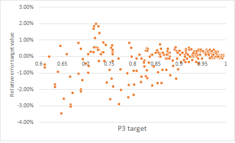
Figure 1: Accuracy of $P_{3}$ approximation

1. The approximation of $P_{3}$ is very accurate for all parameters (cf. figure 1). Errors are highest for low value of the penalty cost $p$, implying a low target value for $P_{3}$.

======== Insert Figure 1 about here ========

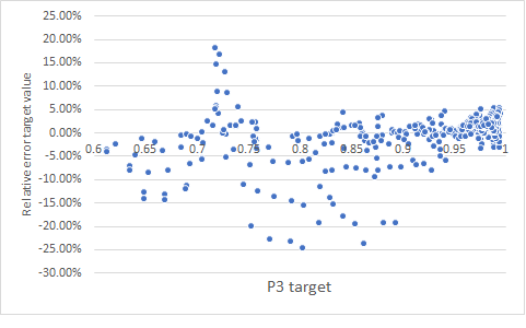
Figure 2: Accuracy of $PIL$ approximation as a function of the $FP_{3}$-target value

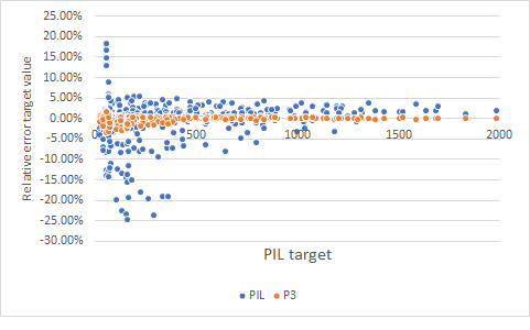
Figure 3: Accuracy of $PIL$ approximation as a function of the $PIL$-target value

2. The approximation of $E[I_{t+L}]$ is less robust (cf. figures 2 and 3). In about $50\%$ of the cases the resulting average inventory from the simulation deviates more than $2\%$ from the target $PIL$. This can be explained by the higher relative errors in the $P_{3}$ approximation for low values of $P_{3}$ and equation (9). In this equation we multiply the approximation for $P_{3}$ with an order quantity and sum $L$ such terms. If the error in these terms are all in the same direction, these errors add up. Errors are largest for cases where the $P_{3}$ target level is below 85%.

======== Insert Figures 2 and 3 about here ========

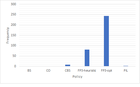
Figure 4: Best policy

3. Despite the approximation errors, the $FP_{3}$-policy is best in $97\%$ of all cases (cf. figure 4) using the SBO methodology. The $BS$-policy was never best. The CO-policy was best in only 1 of the 336 cases. The $CBS$-policy was optimal in $2\%$ (8) of the cases. The $PIL$-policy was best in 2 cases, though, as stated above, this may be caused by the approximation error. The $FP_{3}$-heuristic performed best in $24\%$ of the cases, which we expect to be a result of the approximation error in $P_{3,t+L}$. When using the analytical procedure from de Kok (1989) to determine the cost of the $CO$-policy, the $CO$-policy was best in $9.5\%$ of all cases. We refer to 6 where we show the differences between the costs under the $CO$-policy using the SBO methodology and the analytical approach. Consequently, the $FP_{3}$-policy is best in 88% of the cases, when the analytical solution for the $CO$-policy is substituted for the $CO$-policy from the SBO methodology.

======== Insert Figure 4 about here ========

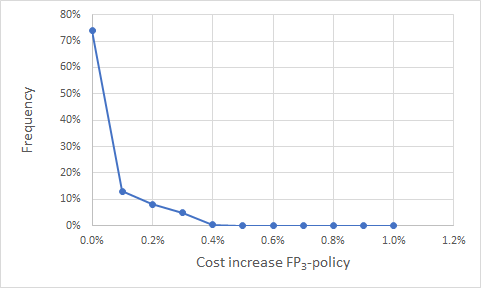
Figure 5: $FP3$ policy against best policy

4. The $FP_{3}$-policy was never more than 0.4% more expensive than the best policy (cf. figure 5. When comparing with the analytically computed costs under the $CO$-policy, the maximum cost increase was $1.3\%$.

======== Insert Figure 5 about here ========

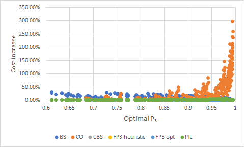
Figure 6: Cost increase with respect to best policy

5. The cost increase of the $CO$-policy can be dramatic compared to the best policy (cf. figure 6). In particular for higher penalty costs, i.e for higher values of the target $P_{3}$ for the optimal $FP_{3}$-policy, cost increase by more than $50\%$.

======== Insert Figure 6 about here ========

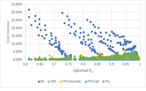
Figure 7: Cost increase with respect to best policy, CO-policy excluded

6. If we exclude the $CO$-policy from our comparison, we conclude that the BS policy is performing much worse than the other four policies, i.e. the $CBS$-policy, the two $FP_{3}$-policies and the $PIL$-policy (cf. figure 7).

======== Insert Figure 7 about here ========

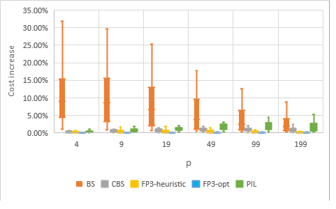
Figure 8: Cost increase with respect to best policy as a function of $p$, $CO$-policy excluded

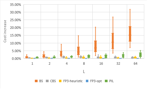
Figure 9: Cost increase with respect to best policy as a function of $L$, $CO$-policy excluded

7. Exploring the performance of the policies further we find, as expected, that the $BS$-policy performs well for high penalty costs (cf. figure 8), but not better than the $CBS$-policy and the $FP_{3}$-policy. However, when lead times are high, the asymptotic optimality of the $BS$-policy for high penalty costs cannot be seen (cf. figure 9). The $CBS$-policy and $FP_{3}$-policy are both very robust, performing very well in comparison with the best policy for all cases.

======== Insert Figures 8 and 9 about here ========

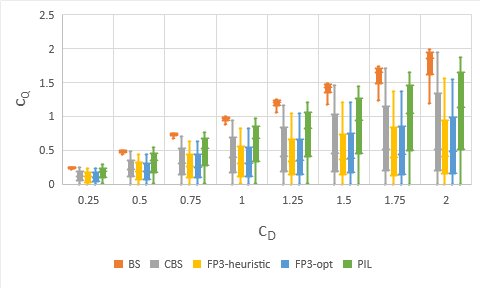
Figure 10: Coefficient of variation of replenishment process as a function of $c_{D}$

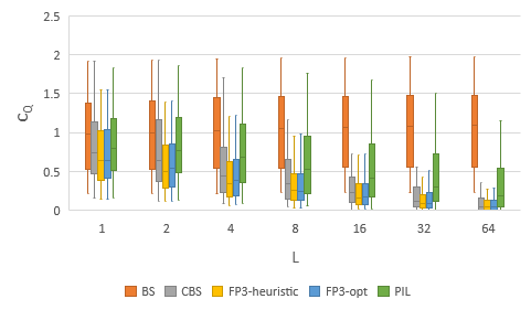
Figure 11: Coefficient of variation of replenishment process as a function of $L$

8. The coefficient of variation of the replenishment order under the $FP_{3}$-policy and $CBS$-policy is substantially lower than the coefficient of variation of the demand per period (cf. figure 10). The replenishment order volatility approaches 0 as lead times get longer, thereby showing that the $FP_{3}$-policy and $CBS$-policy converge to the $CO$-policy as lead times increase. We see a similar effect under the $PIL$-policy, albeit much less pronounced (cf. figure 11).

======== Insert Figures 10 and 11 about here ========

9. We took a closer look at the impact of the (in)accuracy of the $PIL$-target approximation on the cost increase under the approximate $PIL$-policy. Figure ]12 shows that when the approximation error is (very) high, the increase in cost is only limited, below 2%. When the approximation error is small we see costs increases can be 2%-5%. From figures 8 and 9 we see that the $PIL$-policy performs worse for longer lead times and higher penalty costs. We see that $PIL$-target approximation errors are higher for the cases where we applied our heuristic, i.e. cases with $L=32,64$, using the average stock at the start of a period from the $FP_{3}-opt$-policy. Still, we see that even then cost increases are limited for cases with high approximation errors, whereas costs increases can be high for cases with accurate approximations, typically when penalty costs are high.

======== Insert Figure 12 about here ========

6 Conclusions

In this paper we developed new results for the classical periodic review lost-sales model with linear holding and penalty costs. We formulated a new optimality equation that should hold under the optimal policy, despite the fact that this policy is to-date unknown. This optimality equation applies to other policies as well, such as the $CO$-policy and the $FP_{3}$-policy. In the latter case, the optimality equation enables us to find the optimal $FP_{3}$-policy using discrete event simulation. We show that the optimal $FP_{3}$-policy is cost-optimal for the discrete demand cases in Zipkin (2008). The results from our extensive numerical experiment shows the robustness of the $FP_{3}$-policy proposed: the efficient approximation scheme results in a policy that outperforms policies for which asymptotic optimality has been proven formally.
In light of these findings we conjecture that the optimal policy for the lost-sales model considered in this paper is the $FP_{3}$-policy with target $P_{3}$ such that the optimality equation (1) is satisfied. If this conjecture holds true, we unify the optimal policy for both the backlog and lost-sales model as a $FP_{3}$-policy.
We can argue that the policy proposed includes the use of the approximation proposed. Applying the proposed approximation yields a replenishment decision every period. And the experiment shows this decision is effective, even if we do not round off non-integer replenishment quantities under discrete demand.
In line with the observation in van Donselaar et al. (1996), we find a reverse Bullwhip effect for the lost-sales model: a good replenishment policy reduces the volatility in product demand towards the supplier of the product. The positive impact on the upstream supply chain of the volatility reduction found (cf. figures 10 and 11) can not be overstated. Lower replenishment order volatility reduces the need for upstream inventory and reduces production costs.
Both the $CO$-policy and $BS$-policy are not recommended in a real-life setting, as cost increases compared to the costs of the $FP_{3}$-policy can be substantial, in particular for the $CO$-policy.
Our experiments provide further evidence of the excellent cost performance of the $CBS$-policy proposed by Xin (2021). It is essential to cap replenishment quantities in lost-sales systems with lead times of multiple time units. But apparently, this is a built-in feature of the $FP_{3}$-policy. In real-life situations, one can assume a target $P_{3}$ based on tacit knowledge from sales planners, whereafter the policy starts working immediately and caps when needed. Clearly, information about the demand process is required. But with other policies we need to search for the appropriate values of the policy parameters meeting the $P_{3}$-target, too.
Obviously, there is a need for further research. Firstly, the conjecture should be proven or falsified. We expect that a proof starts from assuming that the optimal policy is not an $FP_{3}$-policy, implying that we can distinguish between time points where $P_{3,t+L}$ is greater and smaller than the average $P_{3,t+L}$. By perturbing the optimal policy at these time points, by decreasing and increasing the replenishment quantities, respectively, by some infinitesimal amount, one may show that the perturbed policy reduces costs, which contradicts the optimality of the initial policy.
Secondly, given that the relative error of the $FP_{3}$ approximation scheme can be around $2\%-4\%$, further research on distribution fits could resolve this issue. Equation (7) and its derivation should enable an exact expression for $P_{3,t+L}$ for Mixed Erlang distributions, similar to the exact expression for the fill rate in van Donselaar et al. (1996). Similarly, the recursive scheme based on conditional random variables can be used for exact expressions under discrete demand.
Thirdly, the lost-sales model is a building block of other models, such as transhipments and multiple suppliers, where demand for an item is fulfilled by another source than originally planned for. It may be that the $FP_{3}$-policy can be a building block of policies for such systems. Fourthly, the approximation scheme does not assume demand stationarity, only demand independence in different periods. In a retail environment, demand is non-stationary, as demand on Mondays is typically lower than demand on Fridays and Saturdays. Assuming continuous demand, as we have done in this paper, we can still ensure that each period the target value can be met with a non-negative replenishment. Simulation experiments based on empirical retail data can show the impact of the application of the $FP_{3}$-policy.
As a closing remark, we again advocate the use of the non-stockout probability as the key inventory management performance indicator. It is easy to compute from standard available data, and setting the right target value yields a policy for both the backlog and lost-sales model that is likely to be close-to-optimal.

Comparing simulation and analysis of the CO policy

We noted that the lost-sales model under the $CO$-policy is equivalent to a G/D/1 queue. It is well-known that queueing systems under heavy load, higher than 90%, say, need millions of arriving customers before the system reaches its stationary state. In our SBO methodology we decided to run 100000 time units to determine the long-run average costs for a replenishment policy. In the table below we show that indeed when penalty costs increase, implying a higher fill rate, a higher order quantity, and thereby a higher utilization of the equivalent G/D/1 queue, the difference in SBO long-run costs and analytically derived long -run costs using the moment-iteration method from de Kok (1989) increases. Interestingly, the values of the optimal order quantities do not differ much. Note that, like in our extensive experiment, we assume Mixed Erlang distributed demand.

======== Insert Figure 13 about here ========

Herewith I would like to thank Karel van Donselaar for initiating our work on the lost-sales model after my return to academia in 1992. Ever since, from time to time, we teamed up to work on developing algorithms for real-world problems, and get them implemented in practice. At the time we concluded that base stock policies are no good for lost-sales models and after this paper, our conclusion still stands. I would like to thank Joachim Arts and Willem van Jaarsveld for the many stimulating discussions on policies for the lost-sales model and almost forcing me to complete this paper.

Table 1: Notation

$p$	penalty cost per unit lost
$h$	holding cost per unit on stock at the end of a period
$L$	replenishment lead time
$D_{t}$	demand in period $t$
$Q_{t}$	quantity ordered at the start of period $t$
$I_{t}$	physical inventory at the start of period $t$
$\tilde{I}_{t}$	physical inventory at the end of period $t$
$P_{3,t+L}$	non-stockout probability at the end of period $t+L$,
	determined at the start of period t
$T_{n}$	time between $(n-1)^{th}$ and $n^{th}$ stockout after time 0
$T$	stationary time between stockouts

Table 2: Comparison of polices, Poisson demand

Table 3: Comparison of policies, geometric demand

Table 4: Comparison of exact and approximate PIL-policy

Table 5: Design of discrete event simulation experiment

$p$	4, 9, 19, 49, 99, 199
$h$	1
$L$	1, 2, 4, 8, 16, 32, 64
$c_{D}$	0.25, 0.5, 0.75, 1, 1.25, 1.5, 1.75, 2

Table 6: Comparison of SBO results and analytical results for the $CO$-policy

Figure 12: Impact of $PIL$ approximation error on performance approximate $PIL$-policy

References

- de Kok (1989) de Kok T (1989) A moment-iteration method for approximating the waiting-time characteristics of the gi/g/1 queue. Probability in the Engineering and Informational Sciences 3(2):273–287.
- de Kok (2003) de Kok T (2003) Ruin probabilities with compounding assets for discrete time finite horizon problems, independent period claim sizes and general premium structure. Insurance: Mathematics and Economics 33(3):645–658.
- de Kok (2018) de Kok T (2018) Inventory management: Modeling real-life supply chains and empirical validity. Foundations and Trends® in Technology, Information and Operations Management 11(4):343–437.
- Goldberg et al. (2016) Goldberg DA, Katz-Rogozhnikov DA, Lu Y, Sharma M, Squillante MS (2016) Asymptotic optimality of constant-order policies for lost sales inventory models with large lead times. Mathematics of Operations Research 41(3):898–913.
- Huh et al. (2009) Huh WT, Janakiraman G, Muckstadt JA, Rusmevichientong P (2009) Asymptotic optimality of order-up-to policies in lost sales inventory systems. Management Science 55(3):404–420.
- Silver et al. (2016) Silver EA, Pyke DF, Thomas DJ (2016) Inventory and production management in supply chains (CRC Press).
- Tijms (2003) Tijms HC (2003) A first course in stochastic models (John Wiley and sons).
- van Donselaar et al. (1996) van Donselaar K, de Kok T, Rutten W (1996) Two replenishment strategies for the lost sales inventory model: A comparison. International Journal of Production Economics 46:285–295.
- van Jaarsveld and Arts (2021) van Jaarsveld W, Arts J (2021) Projected inventory level policies for lost sales inventory systems: Asymptotic optimality in two regimes. arXiv preprint arXiv:2101.07519 .
- Xin (2021) Xin L (2021) Understanding the performance of capped base-stock policies in lost-sales inventory models. Operations Research 69(1):61–70.
- Zipkin (2008) Zipkin P (2008) Old and new methods for lost-sales inventory systems. Operations Research 56(5):1256–1263.