CiPR: An Efficient Framework with Cross-instance Positive Relations for Generalized Category Discovery

Abstract

We tackle the issue of generalized category discovery (GCD). GCD considers the open-world problem of automatically clustering a partially labelled dataset, in which the unlabelled data contain instances from novel categories and also the labelled classes. In this paper, we address the GCD problem without a known category number in the unlabelled data. We propose a framework, named CiPR, to bootstrap the representation by exploiting Cross-instance Positive Relations for contrastive learning in the partially labelled data which are neglected in existing methods. First, to obtain reliable cross-instance relations to facilitate the representation learning, we introduce a semi-supervised hierarchical clustering algorithm, named selective neighbor clustering (SNC), which can produce a clustering hierarchy directly from the connected components in the graph constructed by selective neighbors. We also extend SNC to be capable of label assignment for the unlabelled instances with the given class number. Moreover, we present a method to estimate the unknown class number using SNC with a joint reference score considering clustering indexes of both labelled and unlabelled data. Finally, we thoroughly evaluate our framework on public generic image recognition datasets and challenging fine-grained datasets, all establishing the new state-of-the-art.

1 Introduction

After training on large-scale datasets with human annotations, existing machine learning models can achieve superb performance (e.g., [23]). However, the success of these models heavily relies on the fact that they are only tasked to recognize images from the same set of classes with large-scale human annotations on which they are trained. This limits their application in the real open world where we will encounter data without annotations and from unseen categories. Indeed, more and more efforts have been devoted to dealing with more realistic settings. For example, semi-supervised learning (SSL) [5] aims at training a robust model using both labelled and unlabelled data from the same set of classes; few-shot learning [29] tries to learn models that can generalize to new classes with few annotated samples; open-set recognition (OSR) [28] learns to tell whether or not an unlabelled image belongs to one of the classes on which the model is trained. More recently, the problem of novel category discovery (NCD) [15, 13, 12] has been introduced, which learns models to automatically partition unlabelled data from unseen categories by transferring knowledge from seen categories. One assumption in early NCD methods is that unlabelled images are all from unseen categories only. NCD has been recently extended to a more generalized setting, called generalized category discovery (GCD) [34], by relaxing the assumption to reflect the real world better, i.e., unlabelled images are from both seen and unseen categories. The diagram of GCD problem is shown in Fig. 4.

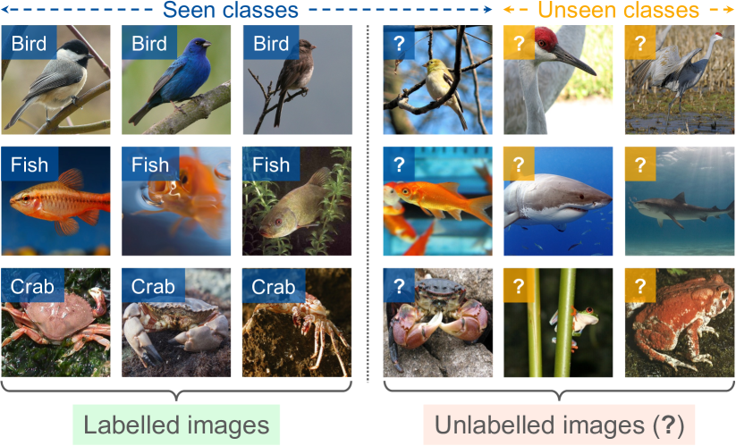
Figure 1: Generalized category discovery: given an image dataset with seen classes from a labelled subset, categorize the unlabelled images, which may come from seen and unseen classes.

In this paper, we tackle the problem of GCD by drawing inspiration from the baseline method [34]. In [34], a vision transformer model was first trained for representation learning using supervised contrastive learning on labelled data and self-supervised contrastive learning on both labelled and unlabelled data. With the learned representation, semi-supervised $k$-means [15] was then adopted for label assignment across all instances. In addition, based on semi-supervised $k$-means, [34] also introduced an algorithm to estimate the unknown category number for the unlabelled data by examining possible category numbers in a given range. However, this approach has several limitations. First, during representation learning, the method considers labelled and unlabelled data independently, and uses a stronger training signal for the labelled data which might compromise the representation of the unlabelled data. Second, the method requires a known category number for performing label assignment. Third, the category number estimation method is slow as it needs to run the clustering algorithm multiple times to test different category numbers.

To overcome the above limitations, we propose a new approach for GCD which does not require a known unseen category number and considers Cross-instance Positive Relations in unlabelled data for better representation learning (CiPR). At the core of our approach is our novel semi-supervised hierarchical clustering algorithm with selective neighbor, named as selective neighbor clustering (SNC), that takes inspiration from the parameter-free hierarchical clustering method FINCH [27]. SNC can not only generate reliable pseudo labels for cross-instance positive relations, but also estimate unseen category numbers without the need for repeated runs of the clustering algorithm. SNC builds a graph indicating all subtly selected neighbor relations constrained by the labelled instances, and produces clusters directly from the connected components in the graph. SNC iteratively constructs a hierarchy of partitions with different granularity, while satisfying the constraints imposed by the labelled instances. With a one-by-one merging strategy, SNC can quickly estimate a reliable class number without repeated runs of the algorithm, which makes it significantly faster than [34].

The main contributions of this paper can be summarized as follows: (1) we propose a new GCD framework, named CiPR, exploiting more cross-instance positive relations in the partially labelled set to strengthen the connections among all instances, fostering the representation learning for better category discovery; (2) we introduce a semi-supervised hierarchical clustering algorithm, named SNC, that can be adopted for reliable pseudo label generation during training and label assignment during testing; (3) we further leverage SNC for class number estimation by exploring intrinsic and extrinsic clustering quality based on a joint reference score considering both labelled and unlabelled data; (4) we comprehensively evaluate our framework on both generic image recognition datasets and challenging fine-grained datasets, and demonstrate state-of-the-art performance across the board.

2 Related work

Our work is related to novel/generalized category discovery, semi-supervised learning, and open-set recognition.

Novel category discovery (NCD) aims at discovering new classes in unlabelled data by leveraging knowledge learned from labelled data. It was pioneered by [15] with a transfer clustering approach. Some earlier works on cross-domain/task transfer learning [17, 18] can also be adopted to tackle this problem. [13] proposed an efficient method called AutoNovel (aka RankStats) using ranking statistics. They first learned a good embedding using low-level self-supervised learning on all data followed by supervised learning on labelled data for higher level features. They introduced a robust ranking statistics to determine whether two unlabelled instances are from the same class for NCD. Several successive works based on RankStats were proposed. For example, [19] proposed to use WTA hashing [37] for NCD in single- and multi-modal data; Zhao and Han [39] extended NCD with dual ranking statistics and knowledge distillation. [12] proposed UNO which uses a unified cross entropy loss to train labelled and unlabelled data. [9] proposed meta discovery which links NCD to meta learning with limited labelled data. [34] introduced generalized category discovery (GCD) which extends NCD by allowing unlabelled data from both old and new classes. They first finetuned a pretrained DINO ViT [4] with both supervised contrastive loss and self-supervised contrastive loss. Semi-supervised $k$-means was then adopted for label assignment. A concurrent work called ORCA by [3] addressed a similar problem by formulating it as open-world semi-supervised learning. We draw inspiration from [34] and develop a novel method to tackle GCD by exploring cross-instance relations on labelled and unlabelled data which is neglected in [34].

Semi-supervised learning (SSL) has long been studied in the machine learning community [5]. It aims at learning a good model by leveraging unlabelled data from the same set of classes as the labelled data. Various methods have been proposed for SSL. For example, $\Pi$-model [24] uses self-ensembling to leverage label predictions on different epochs and under different conditions; Mean Teacher [32] utilizes averaging model weights instead of label predictions; FixMatch [30] and FlexMatch [38] employ pseudo-labels generated from model predictions to guide the training. The assumption that labelled and unlabelled data are from the same closed set of classes is often not valid in practice. In contrast, GCD relaxes this assumption and considers a more challenging scenario where unlabelled data can also come from unseen classes.

Open-set recognition (OSR) aims at training a model using data from a known closed set of classes, and at test time determining whether or not a sample is from one of these known classes. It was first introduced in [28]. Since then many methods have been proposed for this task. For example, OpenMax [1] is the first deep learning work to address the OSR problem based on Extreme Value Theory and fitting per-class Weibull distributions. RPL [7] and its extension ARPL [6] exploit reciprocal points for constructing extra-class space to reduce the risk of unknown. Recently, [35] found the correlation between closed and open-set performance, and boosted the performance of OSR by improving closed-set accuracy. They also proposed Semantic Shift Benchmark (SSB) with a clear definition of semantic novelty for better OSR evaluation.

3 Methodology

3.1 Problem formulation

Generalized category discovery (GCD) aims at automatically categorizing unlabelled images in a collection of data in which part of the data is labelled and the rest is unlabelled. The unlabelled images may come from the labelled classes or new ones. This is a much more realistic open-world setting than the common closed-set classification where the labelled and unlabelled data are from the same set of classes. Let the data collection be $\mathcal{D}=\mathcal{D_{L}}\cup\mathcal{D_{U}}$, where $\mathcal{D_{L}}=\{(x_{i}^{\ell},y_{i}^{\ell})\}^{M}_{i=1}\in\mathcal{X\times Y_{L}}$ denotes the labelled subset and $\mathcal{D_{U}}=\{(x_{i}^{u},y_{i}^{u})\}^{N}_{i=1}\in\mathcal{X\times Y_{U}}$ denotes the unlabelled subset with unknown $y_{i}^{u}\in\mathcal{Y_{U}}$. Only a subset of classes contains labelled instances, i.e., $\mathcal{Y_{L}}\subset\mathcal{Y_{U}}$. The number of labelled classes $N_{\mathcal{L}}$ can be directly deduced from the labelled data, while the number of unlabelled classes $N_{\mathcal{U}}$ is not known a priori.

To tackle this challenge, we propose a novel framework CiPR to jointly learn representations using contrastive learning by considering all possible interactions between labelled and unlabelled instances. Contrastive learning has been applied to learn representation in GCD, but without considering the connections between labelled and unlabelled instances [34] due to the lack of reliable pseudo labels. This limits the learned representation. In this paper, we propose an efficient semi-supervised hierarchical clustering algorithm, named selective neighbor clustering (SNC), to generate reliable pseudo labels to bridge labelled and unlabelled instances during training and bootstrap representation learning. With the generated pseudo labels, we can then train the model on both labelled and unlabelled data in a supervised manner considering all possible pairwise connections. We further extend SNC with a simple one-by-one merging process to allow cluster number estimation and label assignment on all unlabelled instances. An overview of our framework is shown in Fig. 2.

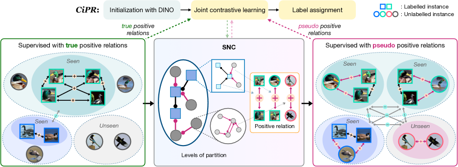
Figure 2: Overview of our CiPR framework. We first initialize ViT with pretrained DINO [4] to obtain a good representation space. We then finetune ViT by conducting joint contrastive learning with both true and pseudo positive relations in a supervised manner. True positive relations come from labelled data while pseudo positive relations of all data are generated by our proposed SNC algorithm. Specifically, SNC generates a hierarchical clustering structure. Pseudo positive relations are granted to all instances in the same cluster at one level of partition, further exploited in joint contrastive learning. With representations well learned, we estimate class number and assign labels to all unlabelled data using SNC with a one-by-one merging strategy.

3.2 Joint contrastive representation learning

Contrastive learning has gained popularity as a technique for self-supervised representation learning [8, 16] and supervised representation learning [20]. These approaches rely on two types of instance relations to derive positive samples. Self-relations are based on whether the paired instances are augmented views from the same image, while cross-instance relations depend on whether the paired instances belong to the same class. For GCD, since the data contains both labelled and unlabelled instances, the mix of self-supervised and supervised contrastive learning appears to be a natural fit and good performance has been reported in [34]. However, cross-instance relations are only considered for pairs of labelled instances, but not for pairs of unlabelled instances and pairs of labelled and unlabelled instances. The learned representation is likely to be biased towards the labelled data due to the stronger learning signal provided by them. Meanwhile, the embedding spaces learned from cross-instance relations of labelled data and self relations of unlabelled data might not be necessarily well aligned. These might explain why a much stronger performance on labelled data was reported in [34] compared with the unlabelled data. To mediate such a bias, we propose to introduce cross-instance relations for pairs of unlabelled instances and pairs of labelled and unlabelled instances in contrastive learning to bootstrap the representation learning. We are the first to exploit labelled-unlabelled relations and unlabelled-unlabelled relations for unbiased representation learning for GCD. To this end, we propose an efficient semi-supervised hierarchical clustering algorithm to generate reliable pseudo labels relating pairs of unlabelled instances and pairs of labelled and unlabelled instances, as will be detailed in Sec. 3.3. Next, we briefly review supervised contrastive learning [20], which accommodates cross-instance relations, and describe how to extend it to unlabelled data.

Contrastive learning objective.

Let $f$ and $\phi$ be a feature extractor and a MLP projection head. The supervised contrastive loss on labelled data can be formulated as

$$\mathcal{L}_{i}^{s}=-\frac{1}{|\mathcal{G_{B}}(i)|}\sum_{q\in\mathcal{G_{B}}(i)}\log\frac{\exp(\boldsymbol{z}^{\ell}_{i}\cdot\boldsymbol{z}^{\ell}_{q}/\tau_{s})}{\sum_{n\in\mathcal{B_{L}},n\neq i}\exp(\boldsymbol{z}^{\ell}_{i}\cdot\boldsymbol{z}^{\ell}_{n}/\tau_{s})}$$ (1)

where $\boldsymbol{z}^{\ell}=\phi(f(x^{\ell}))$, $\tau_{s}$ is the temperature, and $\mathcal{G_{B}}(i)$ denotes other instances sharing the same label with the $i$-th labelled instance in $\mathcal{B_{L}}$, which is the labelled subset in the mini-batch $\mathcal{B}$. Supervised contrastive loss leverages the true cross-instance positive relations between labelled instance pairs. To take into account the cross-instance positive relations for pairs of unlabelled instances and pairs of labelled and unlabelled instances, we extend the supervised contrastive loss on all data as

$$\mathcal{L}_{i}^{a}=-\frac{1}{|\mathcal{P_{B}}(i)|}\sum_{q\in\mathcal{P_{B}}(i)}\log\frac{\exp(\boldsymbol{z}_{i}\cdot\boldsymbol{z}_{q}/\tau_{a})}{\sum_{n\in\mathcal{B},n\neq i}\exp(\boldsymbol{z}_{i}\cdot\boldsymbol{z}_{n}/\tau_{a})}$$ (2)

where $\tau_{a}$ is the temperature, $\mathcal{P_{B}}(i)$ is the set of pseudo positive instances for the $i$-th instance in the mini-batch $\mathcal{B}$. The overall loss considering cross-instance relations for pairs of labelled instances, unlabelled instances, as well as labelled and unlabelled instances can then be written as

$$\mathcal{L}=\sum_{i\in\mathcal{B}}\mathcal{L}_{i}^{a}+\sum_{i\in\mathcal{B_{L}}}\mathcal{L}_{i}^{s}$$ (3)

With the learned representation, we can discover classes with existing algorithms like semi-supervised $k$-means [15, 34]. Besides, we further propose a new method in Sec. 3.4 based on our pseudo label generation approach as will be introduced next.

3.3 Selective neighbor clustering

Although the concept of creating pseudo-labels in Eq. 2 may seem intuitive, effectively realizing it is a challenging task. Obtaining reliable pseudo-labels is a significant challenge in the GCD scenario, and ensuring their quality is of utmost importance. Naive approaches risk producing no performance improvement or even causing degradation. For example, an intuitive approach would be to apply an off-the-shelf clustering method like $k$-means or semi-supervised $k$-means to construct clusters and then obtain cross-instance relations based on the resulting cluster assignment. However, these clustering methods require a class number prior which is inaccessible in GCD task. Moreover, we empirically found that even with a given ground-truth class number, such a simple approach will produce many false positive pairs which severely hurt the representation learning. One way to tackle this problem is to overcluster the data to lower the false positive rate. FINCH [27] has shown superior performance on unsupervised hierarchical overclustering, but it is non-trivial to extend it to cover both labelled and unlabelled data. Experiments show that FINCH will fail drastically if we simply include all the labelled data.

Inspired by FINCH, we propose an efficient semi-supervised hierarchical clustering algorithm, named SNC, with selective neighbor, which subtly makes use of the labelled instances during clustering.

Preliminaries.

FINCH constructs an adjacency matrix $A$ for all possible pairs of instances $(i,j)$, given by

$$A(i,j)=\begin{cases}1&\text{if}\ j=\kappa_{i}\ \text{or}\ \kappa_{j}=i\ \text{or}\ \kappa_{i}=\kappa_{j}\\ 0&\text{else}\end{cases},$$ (4)

where $\kappa_{i}$ is the first neighbor of the $i$-th instance and is defined as

$$\kappa_{i}=\mathop{\arg\max}_{j}\ \{f(x_{i})\cdot f(x_{j})\ |\ x_{j}\in\mathcal{D}\},$$ (5)

where $f(\cdot)$ outputs an $\ell_{2}$-normalized feature vector. A data partition can then be obtained by extracting connected components from $A$. Each connected component in $A$ corresponds to one cluster. By treating each cluster as a super instance and building the first neighbor adjacency matrix iteratively, the algorithm can produce hierarchical partitions.

Algorithm 1 Selective Neighbor Clustering (SNC)

1:Preparation:

2:Given labelled set $\mathcal{D_{L}}$ and unlabelled set $\mathcal{D_{U}}$, treat each instance in $\mathcal{D_{L}}\cup\mathcal{D_{U}}$ as a cluster $\mathbf{c}_{i}^{0}$ with the cluster centroid $\mu(\mathbf{c}_{i}^{0})$ being each instance itself, forming the first partition $\Gamma^{0}=\Gamma_{\mathcal{L}}^{0}\cup\Gamma_{\mathcal{U}}^{0}$, where $\Gamma^{0}=\{\mathbf{c}_{i}^{0}\}_{i=1}^{|\Gamma_{\mathcal{L}}^{0}|+|\Gamma_{\mathcal{U}}^{0}|}$.

3:Main loop:

4:$p\leftarrow 0$

5:while there are more than $N_{\mathcal{L}}$ clusters in $\Gamma^{p}$ do

6:     Initialize $\Gamma^{\star}_{\mathcal{L}}=\Gamma^{p}_{\mathcal{L}}$.

7:     while there exists $\kappa_{i}$ of $\mathbf{c}^{p}_{i}\in\Gamma^{p}_{\mathcal{L}}\cup\Gamma^{p}_{\mathcal{U}}$ not specified do

8:         if $\mathbf{c}^{p}_{i}\in\Gamma^{p}_{\mathcal{L}}$ then

9:              Initialize $\mathcal{Q}=\{\mathbf{c}^{p}_{i}\}$, $\Gamma^{\star}_{\mathcal{L}}=\Gamma^{\star}_{\mathcal{L}}\setminus\{\mathbf{c}^{p}_{i}\}$.

10:              while $|\mathcal{Q}|<\lambda$ do

11:                  $\kappa_{i}\leftarrow\mathop{\arg\max}_{j}\ \{\mu(\mathbf{c}^{p}_{i})\cdot\mu(\mathbf{c}^{p}_{j})\ |\ \mathbf{c}^{p}_{j}\in\Gamma^{\star}_{\mathcal{L}},y^{p}_{j}=y^{p}_{i}\}$

12:                  $\Gamma^{\star}_{\mathcal{L}}\leftarrow\Gamma^{\star}_{\mathcal{L}}\setminus\{\mathbf{c}^{p}_{\kappa_{i}}\}$

13:                  $\mathcal{Q}\leftarrow\mathcal{Q}\cup\{\mathbf{c}^{p}_{\kappa_{i}}\}$

14:                  $\mathbf{c}^{p}_{i}\leftarrow\mathbf{c}^{p}_{\kappa_{i}}$

15:              end while

16:         else

17:              $\kappa_{i}\leftarrow\mathop{\arg\max}_{j}\ \{\mu(\mathbf{c}^{p}_{i})\cdot\mu(\mathbf{c}^{p}_{j})\ |\ \mathbf{c}^{p}_{j}\in\Gamma^{p}_{\mathcal{L}}\cup\Gamma^{p}_{\mathcal{U}}\}$

18:         end if

19:     end while

20:     Construct $A$ following Equation 4 with selective neighbors, forming a new partition $\Gamma^{p+1}=\Gamma^{p+1}_{\mathcal{L}}\cup\Gamma^{p+1}_{\mathcal{U}}$.

21:     $p\leftarrow p+1$

22:end while

Our approach.

First neighbor is designed for purely unlabelled data in FINCH. To make use of the labels in partially labelled data, a straightforward idea is to connect all labelled data from the same class by setting $A(i,j)$ to $1$ for all pairs of instances $(i,j)$ from the same class. However, after filling $A(i,j)$ for pairs of unlabelled instances using Equation 4, very often all instances become connected to a single cluster, making it impossible to properly partition the data. This problem is caused by having too many links among the labelled instances. To solve this problem, we would like to reduce the links between labelled instances while keeping labelled instances from the same class in the same connected component. A simple idea is to connect same labelled instances one by one to form a chain, which can significantly reduce the number of links. However, we found this still produces many incorrect links, resulting in low purity of the connected components. To this end, we introduce our selective neighbor for $\kappa_{i}$ to improve the purity of clusters while properly incorporating the labelled instances, constrained by the following rules. Rule 1: each labelled instance can only be the selective neighbor of another labelled instance once to ensure that labelled instances are connected in the form of chains; Rule 2: we limit the chain length to at most $\lambda$; Rule 3: the selective neighbor of an unlabelled instance depends on its actual distances to other instances, which can be either a labelled or an unlabelled instance. We illustrate how to cluster data with the selective neighbor rules in Fig. 3. Similar to FINCH, we can apply selective neighbor iteratively to produce hierarchical clustering results. We name our method SNC which is summarized in Algorithm 1 (lines 7-19 correspond to selective neighbor computation).

For the chain length $\lambda$, we simply set it to the smallest integer great than or equal to the square root of the number of labelled instances $n_{\ell}$ in each class, i.e., $\lambda=\lceil\sqrt{n_{\ell}}\ \rceil$. This is applied to all classes with labelled instances, and at each hierarchy level. A proper chain length can therefore be dynamically determined based on the actual size of the labelled cluster and also the hierarchy level. We analyze different formulations of chain length in the Appendix.

SNC produces a hierarchy of data partitions with different granularity. Except the bottom level, where each individual instance is treated as one cluster, every non-bottom level can be used to capture cross-instance relations for the level below, because each instance in the current level represents a cluster of instances in the level below. In principle, we can pick any non-bottom level to generate pseudo labels. To have a higher purity for each cluster, it is beneficial to choose a relatively low level which overclusters the data. Hence, we choose a level that has a cluster number notably larger than the labelled class number (e.g., $2\times$ more). Meanwhile, the level should not be too low as this will provide much fewer useful pair-wise correlations. In our experiment, we simply pick the third level from the bottom of hierarchy, which consistently shows good performance on all datasets. We discuss on the impact of the picked level in the Appendix.

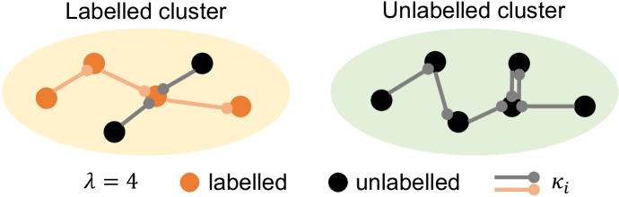
Figure 3: Selective neighbor rules. Left: the labelled instances constitute a chain (rule 1) with the length of $\lambda=4$ (rule 2) and the nearest neighbors of unlabelled instances are labelled ones (rule 3). Right: the nearest neighbors of unlabelled instances are unlabelled ones (rule 3).

3.4 Label assignment

Once a good representation is learned, we could then determine the class label assignment for all unlabelled instances. When the class number is known, we can obtain the label assignment by adopting semi-supervised $k$-means like [15, 34] or directly using our proposed SNC. Since SNC is an hierarchical clustering algorithm and the cluster number in each hierarchy level is determined automatically by the intrinsic correlations of the instances, it might not produce a level of partition with the exact same cluster number as the known class number. We therefore introduce a simple one-by-one merging strategy to SNC allowing it to reach a given class number. Specifically, we first identify a level of partition that has the closest cluster number larger than the given class number, and then merge the clusters one by one until the given class number is reached. At each merging step, we simply merge the two closest clusters. The merging process is summarized in Algorithm 2. The label assignment can then be retrieved from the final partition.

Class number estimation.

When the class number is unknown, exiting methods based on semi-supervised $k$-means need to first estimate the unknown cluster number before they can produce the label assignment. To estimate the unknown cluster number, [15] proposed to run semi-supervised $k$-means on all the data while dropping part of the labels for clustering performance validation. Though effective, this algorithm is computationally expensive as it needs to run semi-supervised $k$-means on all possible cluster numbers. [34] proposed an improved method with Brent’s optimization [2], which increases the efficiency. With the estimated cluster number, semi-supervised $k$-means is run again on all labelled and unlabelled data to produce the final label assignment.

Algorithm 2 One-by-one merging

1:Preparation:

2:Get initial partitions $S=\{\Gamma^{p}\}_{p=0}$ by SNC and a cluster number range $[N_{e},N_{o}]$. Note that the merging is from $N_{o}$ to $N_{e}$ and $N_{o}>N_{e}$.

3:Partition initialization:

4:Find $\Gamma^{t}\in S$ satisfying $|\Gamma^{t}|>N_{o}$ and $|\Gamma^{t+1}|\leq N_{o}$.

5:Merging:

6:while $|\Gamma^{t}|>N_{e}$ do

7:     $(i,j)\leftarrow\mathop{\arg\min}_{i,j}\ \{\mu(\mathbf{c}^{t}_{i})\cdot\mu(\mathbf{c}^{t}_{j})\ |\ \mathbf{c}^{t}_{i},\mathbf{c}^{t}_{j}\in\Gamma^{t}\}$

8:     Merge $\mathbf{c}^{t}_{i}$ and $\mathbf{c}^{t}_{j}$, forming a new partition $\Gamma^{\star}$.

9:     Update current partition $\Gamma^{t}\leftarrow\Gamma^{\star}$.

10:end while

11:Output:

12:Obtain a specific partition $\Gamma^{t}$ of $N_{e}$ clusters, i.e., $|\Gamma^{t}|=N_{e}$.

In contrast, SNC can directly produce hierarchical cluster assignments without a known class number. For practical use, one can pick any level of assignments based on the required granularity. To obtain more reliable class number estimation, we propose to use a joint reference score considering both labelled and unlabelled data. In particular, we further split the labelled data $\mathcal{D_{L}}$ into two parts $\mathcal{D}^{l}_{\mathcal{L}}$ and $\mathcal{D}^{v}_{\mathcal{L}}$. We then run SNC on the full dataset $\mathcal{D}$ treating $\mathcal{D}^{l}_{\mathcal{L}}$ as labelled and $\mathcal{D_{U}}\cup\mathcal{D}^{v}_{\mathcal{L}}$ as unlabelled. We then jointly measure the unsupervised intrinsic clustering index (such as silhouette score [26]) on $\mathcal{D_{U}}$ and the extrinsic clustering accuracy on $\mathcal{D}^{v}_{\mathcal{L}}$. We obtain a joint reference score $s_{c}$ by simply multiplying them after min-max scaling to achieve the best overall measurement on the labelled and unlabelled subsets. We then choose the level in SNC hierarchy with the maximum $s_{c}$.

The cluster number in the chosen level can be regarded as the estimated class number. To achieve more accurate class number estimation, we further leverage the one-by-one merging strategy. Namely, with the chosen level, we apply the one-by-one merging starting from the level below the chosen one to the level above the chosen one. We identify the merge that gives the best reference score $s_{c}$ and its cluster number is considered as our estimated class number.

Our proposed SNC with the one-by-one merging strategy can carry out class number estimation with one single run of hierarchical clustering, which is significantly more efficient than the methods based on semi-supervised $k$-means [15, 35].

4 Experiments

4.1 Experimental setup

Data and evaluation metric.

We evaluate our mothod on three generic image classification datasets, namely CIFAR-10 [22], CIFAR-100 [22], and ImageNet-100 [10]. ImageNet-100 refers to randomly subsampling 100 classes from the ImageNet dataset. We further evaluate on two more challenging fine-grained image classification datasets, namely Semantic Shift Benchmark [35] (SSB includes CUB-200 [36] and Stanford Cars [21]) and long-tailed Herbarium19 [31]. We follow [34] to split the original training set of each dataset into labelled and unlabelled parts. We sample a subset of half the classes as seen categories. $50\%$ of instances of each labelled class are drawn to form the labelled set, and all the rest data constitute the unlabeled set. The model takes all images as input and predicts a label assignment for each unlabelled instance. For evaluation, we measure the clustering accuracy by comparing the predicted label assignment with the ground truth, following the protocol of [34].

Implementation details.

We follow [34] to use the ViT-B-16 initialized with pretrained DINO [4] as our backbone. The output [CLS] token is used as the feature representation. Following the standard practice, we project the representations with a non-linear projection head and use the projected embeddings for contrastive learning. We set the dimension of projected embeddings to 65,536 following [4]. At training time, we feed two views with random augmentations to the model. We only fine-tune the last block of the vision transformer with an initial learning rate of 0.01 and the head is trained with an initial learning rate of 0.1. All methods are trained for 200 epochs with cosine annealing schedule. For our method, the temperatures of two supervised contrastive losses $\tau_{s}$ and $\tau_{a}$ are set to 0.07 and 0.1 respectively. For class number estimation, we set $|\mathcal{D}^{l}_{\mathcal{L}}|$:$|\mathcal{D}^{v}_{\mathcal{L}}|$ = 8:2. Our experiments are conducted on RTX 3090 GPUs.

4.2 Comparison with the state-of-the-art

We compare CiPR with four strong GCD baselines: RankStats+ and UNO+, which are adapted from RankStats [14] and UNO [12] that are originally developed for NCD, the state-of-the-art GCD method of [34], and ORCA [3] which addresses GCD from a semi-supervised learning perspective. As ORCA uses a different backbone model and data splits, for fair comparison, we retrain ORCA with ViT model using the official code on the same splits.

In Sec. 4.2, we compare CiPR with others on the generic image recognition datasets. CiPR consistently outperforms all others by a significant margin. For example, CiPR outperforms the state-of-the-art GCD method of [34] by 6.2% on CIFAR-10, 10.7% on CIFAR-100, and 6.4% on ImageNet-100 for ‘All’ classes, and by 9.5% on CIFAR-10, 22.7% on CIFAR-100, and 12.0% on ImageNet-100 for ‘Unseen’ classes. This demonstrates cross-instance positive relations obtained by SNC are effective to learn better representations for unlabelled data. Due to the fact that a linear classifier is trained on ‘Seen’ classes, UNO+ shows a strong performance on ‘Seen’ classes, but its performance on ‘Unseen’ ones is significantly worse. In contrast, CiPR achieves comparably good performance on both ‘Seen’ and ‘Unseen’ classes, without biasing to the labelled data.

Table 1: Results on generic image recognition datasets.

	CIFAR-10			CIFAR-100			ImageNet-100
Classes	All	Seen	Unseen	All	Seen	Unseen	All	Seen	Unseen
RankStats+ [14]	46.8	19.2	60.5	58.2	77.6	19.3	37.1	61.6	24.8
UNO+ [12]	68.6	98.3	53.8	69.5	80.6	47.2	70.3	95.0	57.9
ORCA [3]	97.3	97.3	97.4	66.4	70.2	58.7	38.2	67.6	23.4
Vaze et al. [34]	91.5	97.9	88.2	70.8	77.6	57.0	74.1	89.8	66.3
Ours (CiPR)	97.7	97.5	97.7	81.5	82.4	79.7	80.5	84.9	78.3

Table 2: Results on fine-grained image recognition datasets.

	CUB-200			SCars			Herbarium19
Classes	All	Seen	Unseen	All	Seen	Unseen	All	Seen	Unseen
RankStats+ [14]	33.3	51.6	24.2	28.3	61.8	12.1	27.9	55.8	12.8
UNO+ [12]	35.1	49.0	28.1	35.5	70.5	18.6	28.3	53.7	14.7
ORCA [3]	35.0	35.6	34.8	32.6	47.0	25.7	24.6	26.5	23.7
Vaze et al. [34]	51.3	56.6	48.7	39.0	57.6	29.9	35.4	51.0	27.0
Ours (CiPR)	57.1	58.7	55.6	47.0	61.5	40.1	36.8	45.4	32.6

In Sec. 4.2, we further compare our method with others on fine-grained image recognition datasets, in which the difference between different classes are subtle, making it more challenging for GCD. Again, CiPR consistently outperforms all other methods for ‘All’ and ‘Unseen’ classes. On CUB-200 and SCars, CiPR achieves 5.8% and 8.0% improvement over the state-of-the-art for ‘All’ classes. For the challenging Herbarium19 dataset, which contains many more classes than other datasets and has the extra challenge of long-tailed distribution, CiPR still achieves an improvement of 1.4% and 5.6% for ‘All’ and ‘Unseen’ classes. Both RankStats+ and UNO+ show a strong bias to the ‘Seen’ classes.

In Fig. 4, we visualize the t-SNE projection on features generated by DINO [4], GCD method of [34], and our method CiPR, performed on CIFAR-10. Both [34] and our features are more discriminative than DINO features. The method of [34] captures better representations with more separable clusters, but some seen categories are confounded with unseen categories, e.g., cat with dog and automobile with truck, while CiPR features show better cluster boundaries for seen and unseen categories, further validating the quality of our learned representation.

Table 3: Estimation of class number in unlabelled data.

	Method	CIFAR-10	CIFAR-100	ImageNet-100	CUB-200	SCars	Herbarium19
Ground truth	—	10	100	100	200	196	683
Estimate (error)	Vaze et al. [34]	9 (10%)	100 (0%)	109 (9%)	231 (16%)	230 (17%)	520 (24%)
	Ours (CiPR)	12 (20%)	103 (3%)	100 (0%)	155 (23%)	182 (7%)	490 (28%)
Runtime	Vaze et al. [34]	15394s	27755s	64524s	7197s	8863s	63901s
	Ours (CiPR)	102s	528s	444s	126s	168s	1654s

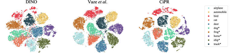
Figure 4: Visualization on CIFAR-10. We conduct t-SNE projection on features extracted by raw DINO, GCD method of [34] and our CiPR. We randomly sample 1000 images of each class from CIFAR-10 to visualize. Unseen categories are marked with *.

4.3 Estimating the unknown class number

In Table 3, we report our estimated class numbers on both generic and fine-grained datasets using the joint reference score $s_{c}$ as described in Sec. 3.4. Overall, CiPR achieves comparable results with the method of [34], but it is far more efficient (40-150 times faster) and also does not require a list of predefined possible numbers. Even for the most difficult Herbarium19 dataset, CiPR only takes a few minutes to finish, while it takes more than an hour for a single run of $k$-means due to large class number, let alone multiple runs from a predefined list of possible class numbers. Both methods have similar memory costs, as reported in the Appendix.

Table 4: Results using different approaches to generate positive relations. Semi-$k$-means^⋆ denotes using semi-supervised $k$-means with an overclustering class number (2 $\times$ ground truth). The results evaluated with SNC are reported of normal size (left), and those with semi-supervised $k$-means are reported of smaller size (right).

	CIFAR-100			CUB-200
Classes	All	Seen	Unseen	All	Seen	Unseen
w/ nearest neighbor	80.4  74.9	82.9  77.5	75.5  69.7	51.9  45.8	56.7  48.2	49.5  44.6
w/ FINCH	81.4  76.6	81.7  75.7	80.7  78.6	51.4  47.9	51.8  45.1	51.3  49.3
w/ k-means	76.7  72.2	77.1  70.4	75.7  75.8	52.8  48.6	53.1  45.5	52.7  50.2
w/ semi-k-means	78.1  73.8	81.5  73.3	71.3  74.8	54.5  48.7	54.1  43.9	54.7  51.2
w/ semi-k-means⋆	76.8  71.9	76.9  71.8	76.4  72.1	56.6  48.1	57.1  50.2	56.4  47.1
w/ SNC (ours)	81.5  76.5	82.4  75.1	79.7  79.3	57.1  50.2	58.7  48.8	55.6  51.0

4.4 Ablation study

Approaches to generate positive relations.

In Table 4, we compare our SNC with multiple different approaches to generate positive relations for joint contrastive learning, including directly using nearest neighbor [40] in every mini-batch and conducting various clustering algorithms to obtain pseudo labels, e.g., FINCH [27], $k$-means [25], and semi-supervised $k$-means [15, 34]. Non-hierarchical clustering methods ($k$-means and semi-supervised $k$-means) require a given cluster number. For $k$-means, we use the ground-truth class number. For semi-supervised $k$-means, we use both the ground truth and the overclustering number (twice the ground truth). We evaluate performance using both proposed SNC and semi-supervised $k$-means for comparison. It is clear that SNC reaches higher accuracy than semi-supervised $k$-means at test time. For generating pseudo positive relations, our method achieves best performance among all approaches. FINCH performs great on CIFAR-100 but degrades on CUB-200. We hypothesize that because FINCH is purely unsupervised without leveraging labelled data, it fails to generate reliable pseudo labels of more semantically similar instances on fine-grained CUB-200. Overclustering semi-supervised $k$-means achieves comparable performance on CUB-200 but performs bad on CIFAR-100. This might be caused by intrinsic poorer performance of semi-supervised $k$-means compared to proposed SNC, which results in worse pseudo labels. We further report the mean purity curve of pseudo labels generated by all clustering methods throughout training process in Fig. 5. We can observe that pseudo labels produced by SNC remain the highest purity on both datasets throughout the entire training process.

Table 5: Results using different relations. $u$-$u$ denotes pair-wise relations between unlabelled and unlabelled data, and $u$-$\ell$ denotes pair-wise relations between unlabelled and labelled data. The results evaluated with SNC are reported of normal size (left), and those with semi-supervised $k$-means are reported of smaller size (right). Rows (3)-(4) mean applying SNC on all data but only using $u$-$u$ or $u$-$\ell$ for pseudo positive relations.

	$k$-means	FINCH	SNC	$u$-$u$	$u$-$\ell$	CIFAR-100			CUB-200
						All	Seen	Unseen	All	Seen	Unseen
(0)	✗	✗	✗	✗	✗	73.6  70.8	80.4  77.6	60.0  57.0	53.1  51.3	57.6  56.6	50.8  48.7
(1)	✓	✗	✗	✓	✗	77.2  73.1	78.3  74.4	74.9  70.7	56.0  51.0	53.8  42.8	57.1  55.2
(2)	✗	✓	✗	✓	✗	80.3  78.2	79.5  76.9	81.7  80.9	51.3  46.1	45.7  40.0	54.0  49.1
(3)	✗	✗	✓	✓	✗	80.5  76.5	80.6  76.3	80.3  76.9	56.6  52.7	57.2  51.5	56.3  53.3
(4)	✗	✗	✓	✗	✓	72.9  70.0	82.0  79.1	54.8  51.6	51.0  45.5	52.9  44.4	50.1  46.0
(5)	✗	✗	✓	✓	✓	81.5  76.5	82.4  75.1	79.7  79.3	57.1  50.2	58.7  48.8	55.6  51.0

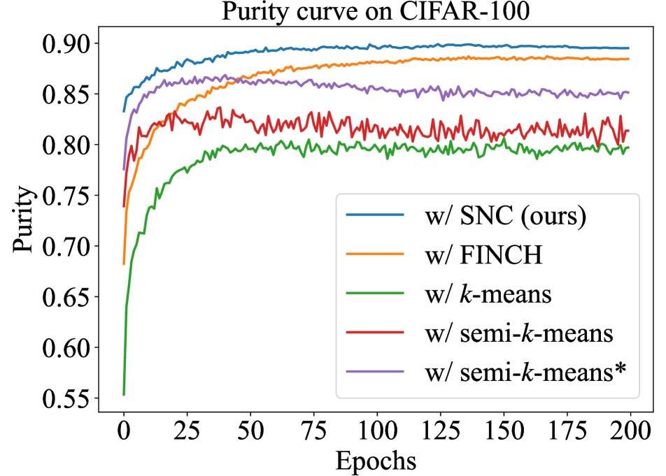
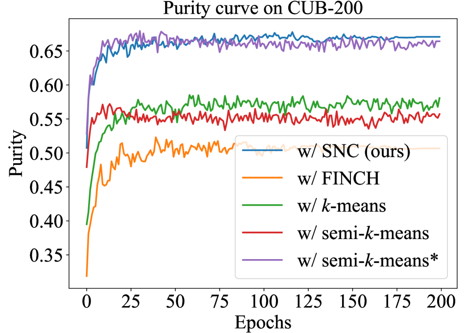
Figure 5: Purity curve. We plot the purity of all compared clustering methods throughout training.

Effectiveness of cross-instance positive relations.

In this paper, we use SNC to generate pair-wise relations of unlabelled data, as well as relations between unlabelled and labelled data in supervised contrastive learning. In Table 5, we evaluate different settings to verify the effectiveness of both of these two relation types. We report evaluation results of SNC and semi-supervised $k$-means, showing higher accuracy achieved by SNC. Row (0) represents the performance of the state-of-the-art GCD method of [34] without using any pseudo relations. Rows (1)-(3) show the effect of using different clustering methods to introduce relations of unlabelled and unlabelled pairs ($u$-$u$). All methods show improvements over [34]. Among all relation-generating methods, SNC brings the largest improvement, outperforming $k$-means and FINCH. Row (4) shows that only adding pair-wise relations of labelled and unlabelled data ($u$-$\ell$) is not sufficient to boost baseline performance. Row (5) is our full method, which achieves the best performance. From (3)-(5), we clearly find fully using relations $u$-$u$ and $u$-$\ell$ generated from SNC benefits our method to the greatest extent, which also substantially improves performance on unseen categories.

5 Conclusion

We have presented a framework CiPR for the challenging problem of GCD. Our framework leverages the cross-instance positive relations that are obtained with SNC, an efficient parameter-free hierarchical clustering algorithm we develop for the GCD setting. Although off-the-shelf clustering methods can be utilized for generating pseudo labels, none of the current methods fulfill all of the fundamental properties of SNC at the same time, critical to GCD. The required properties consist of: (1) using label supervision for clustering unlabeled data, (2) avoiding the need for the number of clusters, and (3) obtaining the highest level of over-clustering purity, which results in reliable pair-wise pseudo labels for unbiased representation learning. With the positive relations obtained by SNC, we can learn better representation for GCD, and the label assignment on the unlabelled data can be obtained from a single run of SNC, which is far more efficient than the semi-supervised $k$-means used in the state-of-the-art method. We also show that SNC can be used to estimate the unknown class number in the unlabelled data with higher efficiency.

Appendix A More analysis on SNC

We present a more detailed illustration of our proposed SNC in Fig. 6. SNC is inspired by the idea from FINCH, but they are significantly different in two key aspects: (1) FINCH treats all instances the same and simply uses nearest neighbors to construct graphs; SNC uses a novel selective neighbor strategy tailored for the GCD setting to construct graphs, treating labelled and unlabelled instances differently. (2) SNC is able to cluster a mixed set of labelled and unlabelled data fully exploiting label supervision, but FINCH is not.

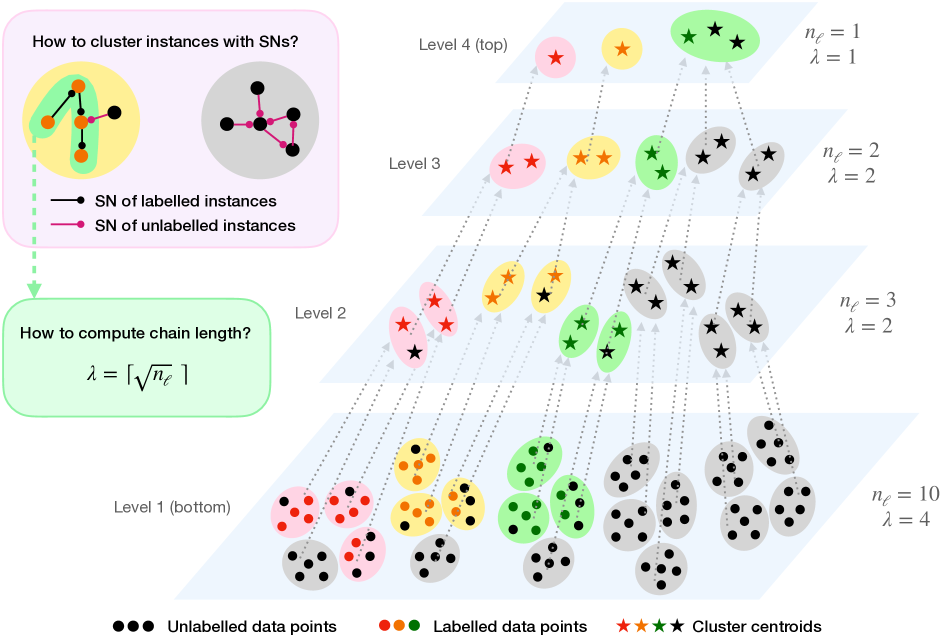
Figure 6: A more detailed illustration of SNC. SNC iteratively clusters instances from the bottom to the top, producing multiple levels of different partitions. At each level, the auto-adaptive chain length $\lambda$ is dynamically determined by the number of labelled ‘instances’ $n_{\ell}$ in each class. The connected components are extracted with selective neighbors (SNs), forming the clusters at each level.

Different choices of chain lengths $\lambda$.

The choice of chain lengths should be positively correlated to (but smaller than) the labelled instance number, while the number should not be too small. The square root used in our paper is the simplest formulation we think of. In Table 6, we experiment on other formulations which satisfies the above relationship, e.g., $\lambda=\lceil\sqrt[3]{n_{\ell}}\ \rceil$ and $\lambda=\lceil n_{\ell}/2\rceil$, and our formulation performs the best. We also compare our dynamic $\lambda$ with a possible alternative of a fixed $\lambda$. For the fixed chain length, we conduct multiple experiments with different length values to find the best length giving the highest accuracy for each dataset. We observe that the best chain length varies from dataset to dataset, and there is no single fixed $\lambda$ that gives the best performance for all datasets. In contrast, our dynamic $\lambda$ consistently outperforms the fixed one, and it can automatically adjust the chain length for different datasets and different levels, without requiring any tuning nor validation like the fixed one.

Table 6: Comparison of different formulations of chain length $\lambda$. The best fixed length values are 8 for CIFAR-100 and 3 for CUB-200.

	CIFAR-100			CUB-200
Classes	All	Seen	Unseen	All	Seen	Unseen
Fixed	80.2	79.7	81.3	54.3	58.8	52.1
$\lceil n_{\ell}/2\rceil$	81.4	84.5	75.2	45.5	45.5	45.5
$\lceil\sqrt[3]{n_{\ell}}\ \rceil$	72.5	77.1	63.2	42.4	45.0	41.1
$\lceil\sqrt{n_{\ell}}\ \rceil$ (ours)	81.5	82.4	79.7	57.1	58.7	55.6

Impacts of different levels for positive relation generation.

A proper level for positive relation generation should overcluster the labelled data to some extent, such that reliable positive relations can be generated. Level 1 is not a valid choice because no positive relations can be generated if each instance is treated as a cluster. In Table 7, we present the performance using levels 2, 3, and 4 to generate pseudo labels and also compare with the previous state-of-the-art baseline by [34]. We empirically find that the overclustering levels 3 and 4 are similarly good, while level 2 is worse because less positive relations are explored in each mini-batch. Even using level 2, our method still performs on par with [34].

Table 7: Comparison of different levels. Compare levels 2, 3, 4, and baseline [34].

	CIFAR-100			CUB-200
Classes	All	Seen	Unseen	All	Seen	Unseen
Baseline [34]	70.8	77.6	57.0	51.3	56.6	48.7
CiPR w/ level 2	72.4	79.6	58.0	50.9	55.8	48.5
CiPR w/ level 3 (ours)	81.5	82.4	79.7	57.1	58.7	55.6
CiPR w/ level 4	81.6	81.9	80.8	52.9	53.1	52.8

Effectivenss of SNC on different learned features.

In Table 8, we evaluate SNC on features extracted from DINO [4], GCD method of [34], and our method CiPR. We also compare SNC with semi-supervised $k$-means [15, 34]. We can observe that SNC surpasses semi-supervised $k$-means with a significant margin on all features, except those extracted by [34] on ImageNet-100. Moreover, semi-supervised $k$-means with our features performs better than with other features. Overall, SNC with our learned features gives the best performance.

Table 8: Effectivenss of SNC on different learned features.

Clustering	Features	CIFAR-100			ImageNet-100			CUB-200			SCars
		All	Seen	Unseen	All	Seen	Unseen	All	Seen	Unseen	All	Seen	Unseen
Semi-$k$-means	DINO [4]	60.4	63.1	54.9	72.8	70.6	73.8	36.7	37.9	36.0	12.3	13.7	11.6
	Vaze et al. [34]	74.5	81.9	60.0	69.2	66.6	70.5	53.5	59.9	50.3	40.8	67.6	27.8
	CiPR (ours)	76.5	75.1	79.3	72.8	70.6	73.8	49.8	46.1	51.7	42.6	55.2	36.5
SNC (ours)	DINO [4]	65.5	69.0	58.3	76.8	81.1	74.6	36.7	35.0	37.5	12.4	15.8	10.7
	Vaze et al. [34]	77.8	87.4	58.6	61.4	76.7	53.8	55.9	61.6	53.0	41.3	62.9	30.8
	CiPR (ours)	81.5	82.4	79.7	80.5	84.9	78.3	57.1	58.7	55.6	47.0	61.5	40.1

Appendix B A unified loss

In this paper, to leverage pseudo labels produced by SNC, we jointly train our model with two supervised contrastive losses, one using true positive relations of labelled data and the other using pseudo positive relations of all data. Indeed, it is possible to train the model with a unified loss by replacing the pseudo relations in the second term of our loss, and remove the first term. Formally, let $\mathcal{R_{B}}(i)$ be the set of positive relations for instance $i$. The unified loss $\mathcal{L}_{i}^{r}$ can be written as

$$\mathcal{L}_{i}^{r} =-\frac{1}{|\mathcal{R_{B}}(i)|}\sum_{q\in\mathcal{R_{B}}(i)}\log\frac{\exp(\boldsymbol{z}_{i}\cdot\boldsymbol{z}_{q}/\tau)}{\sum_{n\in\mathcal{B},n\neq i}\exp(\boldsymbol{z}_{i}\cdot\boldsymbol{z}_{n}/\tau)},$$ (6)

where

$$\mathcal{R_{B}}(i) =\begin{cases}\mathcal{G_{B}}(i)\cup(\mathcal{P_{B}}(i)\cap\mathcal{I_{U}})\quad&\text{if $i\in\mathcal{I_{L}}$}\\ \mathcal{P_{B}}(i)\quad&\text{if $i\in\mathcal{I_{U}}$}\end{cases},$$ (7)

$\mathcal{I_{L}}$ and $\mathcal{I_{U}}$ denote the instance indices of the labelled and unlabelled set respectively. In Table 9, we compare our two-term loss formulation with this unified loss formulation. It turns out that our two-term loss appears to be more effective. We hypothesize the performance degradation of Equation 6 is caused by unbalanced granularity of labelled data and unlabelled data, due to mixture of overclustering pseudo labels and non-overclustering ground-truth labels.

Table 9: Results using different loss formulations..

	CIFAR-100			CUB-200
Classes	All	Seen	Unseen	All	Seen	Unseen
Equation 6	79.3	80.3	77.3	53.9	53.5	54.0
Ours (CiPR)	81.5	82.4	79.7	57.1	58.7	55.6

Appendix C Class number estimation

In Fig. 7, we show how labelled accuracy, silhouette score and reference score change throughout the whole procedure of class number estimation with one-by-one merging. The accuracy on the labelled instances or the silhouette score alone does not well fit the actual cluster number. By jointly considering both, we can see the actual class number aligns well with our suggested reference score.

Figure 7: Curves throughout class number estimation. We report curves of accuracy on the labelled subset $\mathcal{D}^{v}_{\mathcal{L}}$, silhouette score on the unlabelled data $\mathcal{D}_{\mathcal{U}}$, and our reference score on $\mathcal{D}^{v}_{\mathcal{L}}\cup\mathcal{D_{U}}$. Note that the $x$-axis should be read from right to left, as the merging start from the lower level to the upper level.

Appendix D Time efficiency

Here, we evaluate the time efficiency of CiPR, including both category discovery and class number estimation.

Category discovery efficiency.

The latency for the category discovery process mainly consists of two parts: feature extraction and label assignment. In Table 10, we present the feature extraction time. All methods consume roughly the same amount of time for feature extraction per image. RankStats+ [14], UNO+ [12], and ORCA [3] assign labels with a linear classifier, thanks to the assumption of a known category number. Hence, the label assignment process is simply done by a fast feed-forward pass of a linear classifier, costing negligible time ($<0.0005$ second per image), though their performance lags. Our CiPR and [34] contain the transfer clustering process for label assignment, for which CiPR is 6-30 times faster than semi-supervised $k$-means used in [34] (see Table 11).

Table 10: Time cost in feature extraction per image.

	Time cost
RankStats+ [14]	0.015s$\pm$0.001
UNO+ [12]	0.017s$\pm$0.001
ORCA [3]	0.015s$\pm$0.001
Vaze et al. [34]	0.014s$\pm$0.001
Ours (CiPR)	0.014s$\pm$0.001

Table 11: Time and memory cost in clustering.

	CIFAR-10	CIFAR-100	ImageNet-100	CUB-200	SCars	Herbarium19
Semi-$k$-means	346s	688s	3863s	256s	356s	6053s
Ours (SNC w/ one-by-one merging)	58s	111s	118s	36s	50s	917s

Estimating class number.

Compared to repeatedly running $k$-means with different class numbers as in [34], CiPR only requires a single run to obtain the estimated class number, thus significantly increasing efficiency. In Table 12, CiPR is 40-150 times faster than [34], which utilizes $k$-means with the optimization of Brent’s algorithm [2]. We also compare the memory cost. We can observe that our method costs comparable memory but achieves much faster running speed than Vaze et al. [34] in class number estimation.

Table 12: Time and memory consumed in estimating class number.

	Method	CIFAR-10	CIFAR-100	ImageNet-100	CUB-200	SCars	Herbarium19
Runtime (s)	Vaze et al. [34]	15394	27755	64524	7197	8863	63901
	Ours (CiPR)	102	528	444	126	168	1654
Memory (MB)	Vaze et al. [34]	2206	2207	3760	1354	1394	1902
	Ours (CiPR)	2535	2932	5848	1392	1451	2205

Appendix E Attention map visualization

ViT [11] has a multi-head attention design, with each head focusing on different context of the image. For the final block of ViT, the input $\mathbf{X}\in\mathbb{R}^{(HW+1)\times D}$, corresponding to a feature of $HW$ patches and a [CLS] token, is fed into multi-heads, which can be expressed as

$$MultiHead(\mathbf{X})=[head_{1},head_{2},\dots,head_{h}]\mathbf{W}^{O}$$ (8)

where

$$head_{j} =softmax(\frac{\mathbf{Q}_{j}\mathbf{K}_{j}^{T}}{\sqrt{d_{k}}})\mathbf{V}_{j}$$ (9)

$$\mathbf{Q}_{j} =\mathbf{X}\mathbf{W}^{Q}_{j}$$ (10)

$$\mathbf{K}_{j} =\mathbf{X}\mathbf{W}^{K}_{j}$$ (11)

$$\mathbf{V}_{j} =\mathbf{X}\mathbf{W}^{V}_{j}$$ (12)

where $d_{k}$ is the dimension of queries and keys. In our model, patch size is $16\times 16$ pixels and $HW=14\times 14=196$. The number of heads $h$ is $12$. Referring to [33], consider attention map of head $j$ $\mathbf{A}_{j}=softmax(\frac{\mathbf{Q}_{j}\mathbf{K}_{j}^{T}}{\sqrt{d_{k}}})\in[0,1]^{(HW+1)\times(HW+1)}$. $\mathbf{A}_{j}$ describes the similarity of one feature to every other feature captured in head $j$. The first row of $\mathbf{A}_{j}$ shows how head $j$ attends [CLS] token to every spatial patch of the input image. In Fig. 8, we visualize some of the interpretable attention heads to show semantic regions that ViT attends to. We can observe that our model CiPR, as well as DINO [4] and [34], can attend to specific semantic object regions. For instance, CiPR attends three heads respectively to ‘license plate’, ‘light’ and ‘wheels’ for Stanford Cars (head 1 fails in row 1), and to ‘body’, ‘head’ and ‘neck’ for CUB-200.

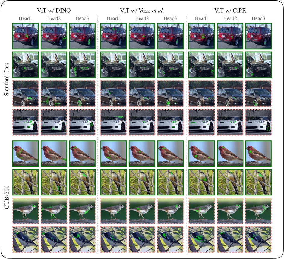
Figure 8: Attention visualizations. We report visualization results of DINO [4] (left), [34] (middle) and CiPR (right) on Stanford Cars (top) and CUB-200 (bottom). For each dataset, we show two rows of ‘Seen’ categories (solid green box) and two rows of ‘Unseen’ categories (dashed red box). Zoom in to see attention details.

Appendix F Data splits

In Table 13, we show the details on data splits of CIFAR-10 [22], CIFAR-100 [22], ImageNet-100 [10], CUB-200 [36], Stanford Cars [21] and Herbarium19 [31] in our experiments.

Table 13: Data splits of all datasets. We present the number of classes in the labelled and unlabelled set ($|\mathcal{Y_{L}}|$, $|\mathcal{Y_{U}}|$), and the number of images ($|\mathcal{D_{L}}|$, $|\mathcal{D_{U}}|$).

	CIFAR-10	CIFAR-100	ImageNet-100	CUB-200	SCars	Herbarium19
$|\mathcal{Y_{L}}|$	5	80	50	100	98	341
$|\mathcal{Y_{U}}|$	10	100	100	200	196	683
$|\mathcal{D_{L}}|$	12.5k	20k	32.5k	1.5k	2.0k	8.5k
$|\mathcal{D_{U}}|$	37.5k	30k	97.5k	4.5k	6.1k	25.7k

Appendix G Special cases of unlabelled data

In the real world, we may meet scenarios where unlabelled data are all from seen or unseen classes. We investigate into such scenarios and conduct experiments to validate the effectiveness of our method. Our experiments are under two settings: (1) applying our pretrained models in the main paper to seen-only and unseen-only unlabelled data; (2) retraining the models with seen-only and unseen-only unlabelled data. In Table 14, we can observe that our model maintains strong performance in all cases.

Table 14: Performance on seen-only and unseen-only unlabelled data. “original setting” denotes the performance of CiPR dealing with GCD; “direct testing” denotes the performance of CiPR dealing with seen-only or unseen-only unlabelled data using pretrained GCD model; “retraining” denotes the performance of retrained CiPR dealing with seen-only or unseen-only unlabelled data.

		CIFAR-10	CIFAR-100	ImageNet-100	CUB-200	SCars	Herbarium19
Seen	original setting	97.5	82.4	84.9	58.7	61.5	45.4
	direct testing	98.5	84.4	83.3	79.1	72.0	55.4
	retraining	98.9	87.0	87.3	81.9	75.2	66.3
Unseen	original setting	97.7	79.7	78.3	55.6	40.1	32.6
	direct testing	97.6	82.7	74.3	56.5	39.3	37.9
	retraining	98.4	78.9	79.3	60.4	42.5	41.3

Appendix H Limitations

We note limitations of our method. In our current experiments, we consider images from the same curated dataset. However, in practice, we might want to transfer concepts from one dataset to another, which may have different data distribution, introducing more challenges. For example, the unlabelled data could follow the long-tailed distribution. Another limitation is that currently, we need to train the model on both labelled and unlabelled data jointly. However, in real world, there are often cases in which we do not have access to any labelled data from the seen classes when facing the unlabelled data. We consider these as our future research directions.

Appendix I License for experimental datasets

All datasets used in this paper are permitted for research use. CIFAR-10 and CIFAR-100 [22] are released under MIT License, allowing for research propose. ImageNet-100 is the subset of ImageNet [10], which allows non-commercial research use. Similarly, CUB-200 [36], Stanford Cars [21] and Herbarium19 [31] are also exclusive for non-commercial research purposes.

References

- [1] Abhijit Bendale and Terrance E Boult. Towards open set deep networks. In CVPR, 2016.
- [2] Richard P. Brent. An algorithm with guaranteed convergence for finding a zero of a function. The Computer Journal, 1971.
- [3] Kaidi Cao, Maria Brbić, and Jure Leskovec. Open-world semi-supervised learning. In ICLR, 2022.
- [4] Mathilde Caron, Hugo Touvron, Ishan Misra, Hervé Jégou, Julien Mairal, Piotr Bojanowski, and Armand Joulin. Emerging properties in self-supervised vision transformers. In ICCV, 2021.
- [5] Olivier Chapelle, Bernhard Scholkopf, and Alexander Zien. Semi-supervised learning. MIT Press, 2006.
- [6] Guangyao Chen, Peixi Peng, Xiangqian Wang, and Yonghong Tian. Adversarial reciprocal points learning for open set recognition. IEEE TPAMI, 2021.
- [7] Guangyao Chen, Limeng Qiao, Yemin Shi, Peixi Peng, Jia Li, Tiejun Huang, Shiliang Pu, and Yonghong Tian. Learning open set network with discriminative reciprocal points. In ECCV, 2020.
- [8] Ting Chen, Simon Kornblith, Mohammad Norouzi, and Geoffrey Hinton. A simple framework for contrastive learning of visual representations. In ICML, 2020.
- [9] Haoang Chi, Feng Liu, Wenjing Yang, Long Lan, Tongliang Liu, Bo Han, Gang Niu, Mingyuan Zhou, and Masashi Sugiyama. Meta discovery: Learning to discover novel classes given very limited data. In ICLR, 2022.
- [10] Jia Deng, Wei Dong, Richard Socher, Li-Jia Li, Kai Li, and Li Fei-Fei. Imagenet: A large-scale hierarchical image database. In CVPR, 2009.
- [11] Alexey Dosovitskiy, Lucas Beyer, Alexander Kolesnikov, Dirk Weissenborn, Xiaohua Zhai, Thomas Unterthiner, Mostafa Dehghani, Matthias Minderer, Georg Heigold, Sylvain Gelly, et al. An image is worth 16x16 words: Transformers for image recognition at scale. arXiv preprint arXiv:2010.11929, 2020.
- [12] Enrico Fini, Enver Sangineto, Stéphane Lathuilière, Zhun Zhong, Moin Nabi, and Elisa Ricci. A unified objective for novel class discovery. In ICCV, 2021.
- [13] Kai Han, Sylvestre-Alvise Rebuffi, Sebastien Ehrhardt, Andrea Vedaldi, and Andrew Zisserman. Automatically discovering and learning new visual categories with ranking statistics. In ICLR, 2020.
- [14] Kai Han, Sylvestre-Alvise Rebuffi, Sebastien Ehrhardt, Andrea Vedaldi, and Andrew Zisserman. Autonovel: Automatically discovering and learning novel visual categories. IEEE TPAMI, 2021.
- [15] Kai Han, Andrea Vedaldi, and Andrew Zisserman. Learning to discover novel visual categories via deep transfer clustering. In ICCV, 2019.
- [16] Kaiming He, Haoqi Fan, Yuxin Wu, Saining Xie, and Ross Girshick. Momentum contrast for unsupervised visual representation learning. In CVPR, 2020.
- [17] Yen-Chang Hsu, Zhaoyang Lv, and Zsolt Kira. Learning to cluster in order to transfer across domains and tasks. In ICLR, 2018.
- [18] Yen-Chang Hsu, Zhaoyang Lv, Joel Schlosser, Phillip Odom, and Zsolt Kira. Multi-class classification without multi-class labels. In ICLR, 2018.
- [19] Xuhui Jia, Kai Han, Yukun Zhu, and Bradley Green. Joint representation learning and novel category discovery on single-and multi-modal data. In ICCV, 2021.
- [20] Prannay Khosla, Piotr Teterwak, Chen Wang, Aaron Sarna, Yonglong Tian, Phillip Isola, Aaron Maschinot, Ce Liu, and Dilip Krishnan. Supervised contrastive learning. In NeurIPS, 2020.
- [21] Jonathan Krause, Michael Stark, Jia Deng, and Li Fei-Fei. 3d object representations for fine-grained categorization. In 4th International IEEE Workshop on 3D Representation and Recognition (3dRR-13), 2013.
- [22] Alex Krizhevsky et al. Learning multiple layers of features from tiny images. Technical report, 2009.
- [23] Alex Krizhevsky, Ilya Sutskever, and Geoffrey E Hinton. Imagenet classification with deep convolutional neural networks. In NeurIPS, 2012.
- [24] Samuli Laine and Timo Aila. Temporal ensembling for semi-supervised learning. In ICLR, 2017.
- [25] James MacQueen et al. Some methods for classification and analysis of multivariate observations. In Proceedings of the fifth Berkeley symposium on mathematical statistics and probability, 1967.
- [26] Peter J. Rousseeuw. Silhouettes: A graphical aid to the interpretation and validation of cluster analysis. Journal of Computational and Applied Mathematics, 1987.
- [27] M. Saquib Sarfraz, Vivek Sharma, and Rainer Stiefelhagen. Efficient parameter-free clustering using first neighbor relations. In CVPR, 2019.
- [28] Walter J Scheirer, Anderson de Rezende Rocha, Archana Sapkota, and Terrance E Boult. Toward open set recognition. IEEE TPAMI, 2012.
- [29] Jake Snell, Kevin Swersky, and Richard Zemel. Prototypical networks for few-shot learning. In NeurIPS, 2017.
- [30] Kihyuk Sohn, David Berthelot, Nicholas Carlini, Zizhao Zhang, Han Zhang, Colin A Raffel, Ekin Dogus Cubuk, Alexey Kurakin, and Chun-Liang Li. Fixmatch: Simplifying semi-supervised learning with consistency and confidence. In NeurIPS, 2020.
- [31] Kiat Chuan Tan, Yulong Liu, Barbara A. Ambrose, Melissa Tulig, and Serge J. Belongie. The herbarium challenge 2019 dataset. arXiv preprint arXiv:1906.05372, 2019.
- [32] Antti Tarvainen and Harri Valpola. Mean teachers are better role models: Weight-averaged consistency targets improve semi-supervised deep learning results. In NeurIPS, 2017.
- [33] Ashish Vaswani, Noam Shazeer, Niki Parmar, Jakob Uszkoreit, Llion Jones, Aidan N Gomez, Łukasz Kaiser, and Illia Polosukhin. Attention is all you need. In NeurIPS, 2017.
- [34] Sagar Vaze, Kai Han, Andrea Vedaldi, and Andrew Zisserman. Generalized category discovery. In CVPR, 2022.
- [35] Sagar Vaze, Kai Han, Andrea Vedaldi, and Andrew Zisserman. Open-set recognition: A good closed-set classifier is all you need. In ICLR, 2022.
- [36] Catherine Wah, Steve Branson, Peter Welinder, Pietro Perona, and Serge Belongie. The caltech-ucsd birds-200-2011 dataset. Technical report, 2011.
- [37] Jay Yagnik, Dennis W. Strelow, David A. Ross, and Ruei-Sung Lin. The power of comparative reasoning. In ICCV, 2011.
- [38] Bowen Zhang, Yidong Wang, Wenxin Hou, Hao Wu, Jindong Wang, Manabu Okumura, and Takahiro Shinozaki. Flexmatch: Boosting semi-supervised learning with curriculum pseudo labeling. In NeurIPS, 2021.
- [39] Bingchen Zhao and Kai Han. Novel visual category discovery with dual ranking statistics and mutual knowledge distillation. In NeurIPS, 2021.
- [40] Zhun Zhong, Enrico Fini, Subhankar Roy, Zhiming Luo, Elisa Ricci, and Nicu Sebe. Neighborhood contrastive learning for novel class discovery. In CVPR, 2021.