Quasi-binary encoding based quantum alternating operator ansatz
Abstract
This paper proposes a quasi-binary encoding based algorithm for solving a specific quadratic optimization models with discrete variables, in the quantum approximate optimization algorithm (QAOA) framework. The quadratic optimization model has three constraints: 1. Discrete constraint, the variables are required to be integers. 2. Bound constraint, each variable is required to be greater than or equal to an integer and less than or equal to another integer. 3. Sum constraint, the sum of all variables should be a given integer.
To solve this optimization model, we use quasi-binary encoding to encode the variables. For an integer variable with upper bound and lower bound , this encoding method can use at most qubits to encode the variable. Moreover, we design a mixing operator specifically for this encoding to satisfy the hard constraint model. In the hard constraint model, the quantum state always satisfies the constraints during the evolution, and no penalty term is needed in the objective function. In other parts of the QAOA framework, we also incorporate ideas such as CVaR-QAOA and parameter scheduling methods into our QAOA algorithm.
In the financial field, by introducing precision, portfolio optimization problems can be reduced to the above model. We will use portfolio optimization cases for numerical simulation. We design an iterative method to solve the problem of coarse precision caused by insufficient qubits of the simulators or quantum computers. This iterative method can refine the precision by multiple few-qubit experiments.
Keywords Quantum approximate optimization algorithm Quantum alternative operator Ansatz Portfolio optimization
1 Introduction
Quantum computing is an emerging field that aims to harness the power of quantum phenomena to perform computations beyond the capabilities of classical computers. The field traces its origins to the 1980s, when Richard Feynman suggested the possibility of using quantum systems to simulate complex physical processes [1]. Since then, quantum computing has become an interdisciplinary field that involves physics, computer science, chemistry, biology, etc [2, 3, 4, 5, 6].
A near-term major challenge in quantum computing is to develop algorithms that can run on noisy intermediate-scale quantum (NISQ) devices. Quantum heuristics algorithms, including quantum approximate optimization algorithm (QAOA) [7], variational quantum eigensolver (VQE) [8] and quantum annealing (QA) [9], are a type of algorithms that are tailored for NISQ devices. These algorithms are designed to be resilient to noise and other sources of error in the quantum hardware, making them suitable for NISQ devices.
As one of the most prominent quantum heuristics algorithms, QAOA is designed to solve combinatorial optimization problems. The algorithm has demonstrated its effectiveness on various problems, such as MaxCut [7], MaxSat [10], and graph partitioning [11]. QAOA is expected to play a key role in the development of real-world quantum applications.
QAOA for solving constrained combinatorial optimization can be divided into two models: the soft constraint model and the hard constraint model [10, 12]. The soft constraint model incorporates the constraints into the objective function as penalty terms, which can be adjusted by a penalty factor. However, choosing an appropriate penalty factor is challenging, as it affects the balance between feasibility and optimality of the solutions [13, 14]. When the penalty factor is large, the model tends to output solutions that satisfy the constraint conditions, while ignoring the differences in the value of the original objective function. On the contrary, when the penalty factor is small, the probability of infeasible solutions output by the model will increase. The hard constraint model, also known as quantum alternating operator ansatz [10] or QAOAz [15] or C-QAOA [16], ensures that the quantum state represents a feasible solution by designing operators that control the qubit evolution. This model has a higher chance of finding the optimal solution, but it is more complex to implement.
QAOAz algorithms are widely used to solve combinatorial optimization problems with binary variables, such as Max Cut and Traveling Salesman Problem [10]. In these problems, variables are only represented by 0 and 1, indicating one of two options. Therefore, QAOAz algorithms do not need a specific encoding method for these problems. However, some more practical optimization models, such as portfolio optimization problems in the financial field [12, 17], will involve integer encoding to represent the number of shares . One of the main challenges for applying QAOAz to this kind of problem is that the existing encoding methods are inefficient, as the qubits increase linearly to represent more choices, which results in limited scale and precision of the problem solving. For instance, the current state-of-the-art such as Hodson’s enoding [12] or quantum-walk QAOA (QW-QAOA) [15] only consider three discrete positions for portfolio optimization: long, short, and no position, rather than the percentage of investment or integer shares. Another challenge is that other efficient encoding methods (such as binary encoding or Palmer encoding [17]) do not accommodate hard constraints, because it is difficult to construct a QAOAz mixer that satisfies the encoding rule. Although some general QAOAz mixer preparation methods [18, 19] have emerged, or there are some improvement schemes for the solution quality of soft constraint methods [20, 21, 22], these schemes are difficult to implement effectively on the business side due to efficiency issues or their own assumptions.
This paper will propose a quasi-binary encoding based QAOA (QB-QAOA) that aims to solve a quadratic optimization problem with integer variables in hard constraint way. The constraints of the model involve the sum constraint and bound constraint of integer variables. The optimization model can be written as:
| (1) | ||||
where is the number of the integer variables in the model, denotes the -th variable, and denote the lower bound and upper bound of , and is the sum of all elements in .
To convert the integer variables to decimal variables, we define a new parameter whose value is equal to , which represents the precision coefficient of the variables. By multiplying both sides of the constraints by , we can rewrite some of the parameters and variables as follows:
| (2) | ||||
| (3) | ||||
Equation 3 is analogous to the Markowitz model [23] for portfolio optimization, which can assist investors in optimizing their portfolio by trading off risk and return. Here, represents the covariance of historical interest rates between asset and asset , and denotes the expectation of historical interest rate for asset . When we expect to use QAOA to solve the portfolio optimization problem with percentage weights, we pre-determine a parameter coefficient , whose reciprocal is an integer, and then transform Equation 3 into Equation 1 to solve.
QB-QAOA requires only qubits to represent each variable . Moreover, we propose a novel mixing operator for QB-QAOA, which has a circuit depth ranging from constant to linear depending on the problem structure. In the numerical simulation, we apply QB-QAOA to the portfolio optimization problem, and also introduce CVaR-QAOA [24] and parameter scheduling techniques [21] to enhance the solution quality. We also propose a precision increasing iterative method, which is motivated by the fact that the current real quantum computers or simulators cannot provide enough qubits to perform precise calculations. During the iterative process, our iterative method initially uses coarse precision (large in Equation 2) for operations, before subsequently increasing the precision ( gets smaller) while maintaining the same qubits count.
The paper is organized as follows: In Section 2, we introduce the fundamental concepts the QAOA framework. In Section 3, we present the Quasi-Binary based QAOA algorithm including the design of quasi-binary encoding and mixing operator. In Section 4, we provide a series of numerical simulations to evaluate the performance of QB-QAOA. In Section 5, we present the precision increasing iterative method and corresponding simulation results. In Section 6, a conclusion is presented.
2 Quantum Approximate Optimization Algorithm Framework
There are four main components in QAOA framework: encoding, initial states, phase-separation operator, and mixing operator.
2.1 Encoding
The encoding is the process of mapping the solutions of a problem to quantum states and reading the outcomes of qubit measurements as solutions. The purpose of encoding is to represent decimal or integer variables in an optimization model using binary variables. The encoding also determines how many qubits are needed for each asset. In a hard constraint model, the encoding also influences the difficulty to design the mixing operator.
The encoding of QAOA varies depending on the application of interest. For example, for the maxcut problem, the encoding is straightforward, with 0 and 1 representing different sets of vertices. For portfolio optimization, the encoding uses the qubits to express integers. Binary and one-hot encoding are often used to present one integer variable. The number of qubits required for the former scales logarithmically with the range of integers represented, while the latter scales linearly.
Besides binary and one-hot encoding, QAOA encoding also includes domain wall encoding [25], Hodson encoding [12], Quantum Walk encoding [15], Palmer encoding [17], etc. Domain wall encoding can save one qubit for each discrete variable and only requires linear connections instead of full connections between qubits compared with one-hot encoding [25]. Hodson encoding, Palmer encoding, and Quantum Walk encoding are only suitable for portfolio optimization problems. Hodson encoding uses two qubits to represent the encoding state of each position, where 01 means long position (1), 10 means short position (-1), 00 and 11 mean no position (0) [12]. When the choices of the variable increase, for example, if , 4 qubits should be used, such as 0101 represents 2 or 1010 represents -2. Therefore, the number of qubits for each variable will increase linearly as the choice of that variable increases. Quantum Walk encoding can encode across assets and assign a number to each valid portfolio starting from 0, making it the most efficient [12]. However, since Quantum Walk encoding cannot independently compute the phase separation operator, it still relies on the Hodson encoding circuit. Palmer encoding is specially designed for bound constraints, and its number of qubits is at most one more than binary encoding [17], but it does not support hard constraint models.
To our knowledge, our quasi-binary encoding is the only encoding in QAOA that satisfies the following three conditions simultaneously. First, it only requires a logarithmic number of qubits to represent a variable, where the logarithm is based on the number of possible values of the variable. Second, it can handle bound constraints on the variable values. Third, it can be implemented in the hard constraint model, which ensures that only feasible solutions are considered.
2.2 Initial State
The initial state () is a quantum state that usually represents one or more feasible solutions. The circuit for the initial state is recommanded as a constant-depth circuit, often composed of several X gates [10]. In some literatures [26, 27, 28], a warm-starting method is used, which finds an initial continuous solution that is closer to the discrete optimal solution by using a classical method, thereby reducing the optimization time in subsequent steps.
2.3 Phase-Separation Operator
The phase-separation operator () is an operator to relate the objective function to the quantum circuit, which is usually a diagonal unitary matrix in the computational basis. The phase-separation operator can be written as , where is the phase-separation Hamiltonian, and is a circuit parameter. The encoding method and the cost function collectively determine how to construct .
The general procedure to construct the phase-separation Hamiltonian involves the following steps:
-
•
Reformulate the objective function to the binary objective function whose variables are binary variables according to the chosen encoding method.
-
•
Substitute in the equation, transforming it into a cost function with the variable vector .
-
•
Replace with the Pauli Z matrix and the products between in the cost function with tensor products. The phase-separation Hamiltonian is the value of the new cost function, which is a matrix, where is the number of or qubits.
In soft constraint models, the objective function becomes more complex, and constraints are usually added to the objective function as penalty terms. If constraints are equality constraints, the penalty term is the sum of the squares of the difference between the left and right sides of the equations. If the constraint is an inequality constraint, slack variables need to be introduced, which makes the model even more complex [22, 29, 30].
In theory, multiplying the Hamiltonian by a constant does not change the solution to the problem. However, in real experiments, we need to use classical optimizers to optimize the phase-separation operator parameter and the mixing operator . To ensure that the optimizer’s learning rate is consistent, we need to multiply a suitable parameter on the Hamiltonian to synchronize the steps of and . Some references have given the calculation methods for [21, 31].
2.4 Mixing Operator
The mixing operator (), also known as mixer is an operator that modifies the quantum state of the system and allows it to explore different regions of the solution space. The choice of the mixing operator depends on the problem structure and the optimization goal. If it is not necessary to distinguish whether the explored region is feasible or not, a common choice is the RX gate [7]. However, other operators may be more suitable for some problems, such as the XY-mixer, to transfer the quantum states among one-hot states or Dicke states [10]. The design of the mixing operator will determine whether the QAOA algorithm is implemented in a soft constraint or a hard constraint manner.
In hard constraint model, let be the set of quantum states that represent all feasible solutions. Then, must satisfy the condition that there exists a parameter such that for all [10]. A common choice for is to use the exponential of a mixing Hamiltonian , such that . Fuchs et al. developed a general method to find Hamiltonian given [19]. However, this method requires knowing the entire set , which is often impractical or impossible. Thus, this method would negate the quantum speedup. Moreover, the method of Fuchs et al. [19] only guarantees the correct evolution of states within . For states outside , the resulting states are unpredictable. Therefore, this method cannot handle partial qubits.
However, constructing Hamiltonian is not the essential way to build a mixing operator circuit. Brtschi et al. presented the Grover mixer [18], which is based on the quantum gate that can transform into an equal superposition of all feasible solutions. However, for Eq. 2, it is still very difficult to create such a quantum gate. In this paper, we propose a novel mixing operator for QB-QAOA and use the idea of quantum chemistry circuit design [32, 33] to decompose it into CNOT gates and multi-control RX gates.
2.5 Objective Function Estimation
According to the above four components, the QAOA circuit consists of an initial circuit and layers of phase separation operator circuits and mixing operator circuits, where is the depth parameter. The final state produced by the circuit is written as . Then, a classical optimizer is used to find the optimal values of and that minimize the QAOA objective function .
In some special objective functions, such as the max-cut problem and the Sherrington-Kirkpatrick Model, the objective function has an analytical solution when is small [7, 34], so the optimal parameters can be quickly obtained by differential-based methods. However, in some general cases, it is difficult to calculate . In this paper, we will present two methods for estimating it: Normal-QAOA and CVaR-QAOA [24].
Normal-QAOA uses the following for estimation:
| (4) |
where denotes the number of measurements, which is set to in our simulation, represents the value of the variable obtained by the -th measurement results, and Cost is the cost function defined in Equation 7. Therefore, Equation 4 means the average cost of all samples.
CVaR-QAOA [24] uses the following for estimation:
| (5) |
where is the tail rate, and the value is 0.05 in our simulation. Equation 5 represents the average cost for the best 5% samples. According to the Ref. [24], when the optimization objective focuses on the optimal solution rather than the average performance of all solutions, CVaR-QAOA performs better than Normal-QAOA.
2.6 Parameter Scheduling
Since using classical optimization algorithms [35, 36, 37, 38, 39] to find the global optimal parameters of is computationally expensive [40, 41, 42, 43], parameter scheduling methods are usually used to optimize the parameters [44, 45, 46, 31, 47]. Parameter scheduling methods usually assume that the optimal parameters satisfy certain rules, or that the optimal parameters of one instance can be inferred from the optimal parameters of instances similar to it. Parameter scheduling methods may not find the global optimal parameters, but they can find good suboptimal parameters within an acceptable time. In this paper, we will use four parameter scheduling methods in simulation experiments to estimate the optimal parameters.
- •
-
•
Optimized linear schedule (OLS): According to the theory in Ref. [48], the optimal parameters increase linearly with . We then use the two parameters, and , shown in Equation 6 to represent the original parameters. Based on Ref. [21], these two new parameters are optimized first. Then, according to the optimization results, we solve for the values of the original parameters and use them as initial values for further optimization.
(6) -
•
Iterative optimized linear schedule (IOLS) [21]: The main idea of IOLS is to use the optimal parameters of a lower-layer QAOA as a guide for finding the optimal parameters of a higher-layer QAOA. Let be the coordinate of the -th parameter in the -layer QAOA, as defined in Equation 6. Given the optimal parameters of the -layer QAOA, and , we can find two integers, and , such that and are the nearest neighbors of among all the coordinates in the -layer QAOA. IOLS assumes that the optimal parameters of the -layer QAOA lie on the same line as the optimal parameters of the -layer QAOA at the corresponding positions. That is, the points (, ), (, ) and (, ) are on a straight line, and so are the points (, ), (, ) and (, ). Based on this assumption, we can use linear interpolation to estimate and from and . These estimates are then used as initial values for further optimization.
-
•
Iterative QAOA (IQAOA) [21]: IQAOA is also based on the iterative method. The main idea is to use the optimal parameters of the -layer QAOA as the initial values of the -layer QAOA, except for the last parameter of and , which is set to zero. Then, the next step is to refine the initial value with a further optimization.
3 Quasi-Binary Based QAOA
To solve Equation 1, we introduce a new variable for all , and then use to rewrite Equation 1 as follows:
| (7) | ||||
The objective function in Equation 7 is still a quadratic form, and the discrete constraint, the bound constraint and the sum constraint have not changed significantly. After introducing the following parameters:
| (8) | ||||
Equation 7 is transferred into:
| (9) | ||||
In this section, we will present QB-QAOA to solve the optimization model as Equation 9.
3.1 Quasi-Binary Encoding
Based on Equation 9, the encoding method should encode , within a range of 0 to . The tradtional binary encoding is not a good choice, when for . To address this issue, we propose the quasi-binary encoding. The quasi-binary encoding is denoted as
| (10) | ||||
| where | ||||
In Equation 10, denotes the floor of , and denotes the -th bit of the -length binary number of . For example, if , then , so , , and . Therefore, the encoding function is:
| (11) |
The variable is encoded with five bits: one for 1, two for 2, one for 4, and one for 8. If all bits are 1, the value is , which is the maximum. If all bits are 0, the value is zero, which is the minimum. It is clear that the quasi-binary encoding method can represent any positive integer from 0 to . This is because when , we can encode with the partial bits in a binary encoding way. When , we set all the bits in to 1, and encode with bits in a binary encoding way.
In some special cases where the gaps between of some variables are very large, quasi-binary encoding needs further improvement to adapt to the design of the mixing operator we will introduce later. The mixing operator will operate on one -qubit and two -qubits for all 111We use -qubit to denote the qubit that represents .. Hence, we need to ensure that the total number of -qubits in all variables should be at least 2, except for the qubit that represents the highest power of 2 (denoted as ). To achieve this, after computing and as Equation 10 for each , we count how many -qubits are in all variables for each from 1 to . If the number is less than 2, we split one -qubit into two -qubits in the same variable. This transformation results in a finer split of integers, and does not affect the upper bounds of the variables.
As , we can use at most qubits to represent the value, where . Even if some qubits are splitted to adapt the mixing operator, the total number of qubits for all variables will not exceed . Therefore, the number of qubits for a variable is logarithmic in the number of its possible values.
3.2 Initial State
To generate the initial quantum state, we must first obtain a feasible solution that satisfies the conditions and . To accomplish this, we utilize the greedy allocation method, as outlined in Algorithm 1:
Here, denotes the subarray spanning from to . Subsequently, is encoded into a binary sequence with quasi-binary encoding and is applyed to a quantum circuit with X gates. The greedy allocation method chooses the largest value in the range for the first few variables, which means that the first few qubits are affected by X gates in the initial circuit.
In this section, we have shown one way to create valid solutions. Any quantum state that corresponds to a valid solution under this encoding can be used.
3.3 Phase Separation Operator
3.4 Mixing Operator
The mixing operator Hamiltonian of QB-QAOA can be expressed as:
| (12) | ||||
where , , represent the Pauli operators acting on the -th qubit and represents the number represented by the -th qubit.
The measurement result of the mixer operated on is shown in Figure 1, where Hamiltonian is defined by Equation 12 in a 6-qubit system and . In this system, the first three qubits represent 1, the fourth and fifth qubits represent 2, and the sixth qubit represents 4. Initially, the sixth qubit is initialized to , while the others are initialized to , which means the initial sum is 4. After applying the Hamiltonian for , the final state is measured 10,000 times. The results are shown in Figure 1, which indicates that the system only transitions to states that have a sum of 4, as expected from the sum constraint.
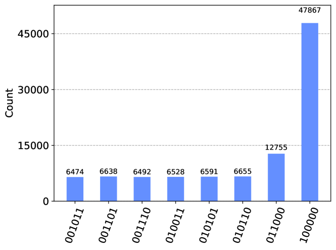
However, a complete mixer can not handle a large number of qubits, so we use the ring mixer to build the circuit [13, 14]. The circuit has two components, each corresponding to one of the terms in Equation 12. The first component implements the ring XY mixer, and the second component implements the ring XYY mixer.
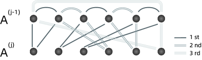
Figure 2a illustrates the circuit realization of a two-qubit XY-mixer, which partially swaps the states and . The XY-mixers operate on qubits that have the same integer value in the quasi-binary encoding. For example, if we have as the set of qubits to represent , the ring XY-mixer will be operated on these qubits in a certain order based on the literature [10]. Figure 2b explains how this works when has 6 qubits. The implementation of the ring XY-mixer is divided into three rounds, and in each round, the XY-mixers act on the qubits at the ends of the arc in Figure 2b.
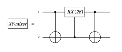
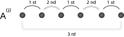
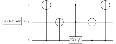
Figure 3a shows how to build a three-qubit XYY-mixer circuit, which partially swaps the states and . XYY-mixers work on two qubits to represent (the first and second qubits) and one qubit to represent (the third qubit). Given that the XYY-mixers work on the qubits in and , which are the sets of qubits that represent and , respectively. Figure 3b shows the order of applying the XYY-mixer to these qubits. The ring XYY-mixer has also three rounds, like the ring XY-mixer. The way of choosing two qubits from is the same as the XY-mixer in Figure 2b. After picking the two qubits from , the XYY-mixer picks one single qubit from that have not been picked yet.
We assume that both and have six qubits in Figure 3b. But in reality, the number of qubits in does not depend on the number of qubits in , so there might be more or less qubits in when we pair them up. If there are not enough qubits in , we can use the qubits that have been picked before for the XYY-mixer. If there are extra qubits in , we can ignore them.
Algorithm 2 gives the construction process of the whole mixer circuit. The pairing methods and order shown in Figure 2b and Figure 3b are also given more clearly in pseudocode. The depth of the whole mixing circuit is , where and are the size of and .
4 Numerical Simulation
4.1 Data and parameter
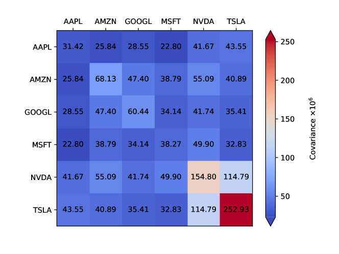
We applied the QB-QAOA method to optimize a portfolio of six NASDAQ stocks (AAPL, AMZN, GOOGL, MSFT, NVDA, TSLA) using Qiskit. We used the historical returns rates of these stocks as the input data. Table 1 shows the expected returns and Figure 4 shows the covariance matrix of the stocks.
| Stock | AAPL | AMZN | GOOGL | MSFT | NVDA | TSLA |
|---|---|---|---|---|---|---|
| Returns Expectation | 0.134 ‰ | 0.354 ‰ | -1.582 ‰ | -0.152 ‰ | 6.261 ‰ | 2.187 ‰ |
The risk factor is setted as 18.415, so according to the Appendix A, we get the minimum target return of exactly 2 ‰. The values of the precision parameter , the lower bound , and the upper bound depend on the simulation content and may change accordingly.
4.2 Qubits count
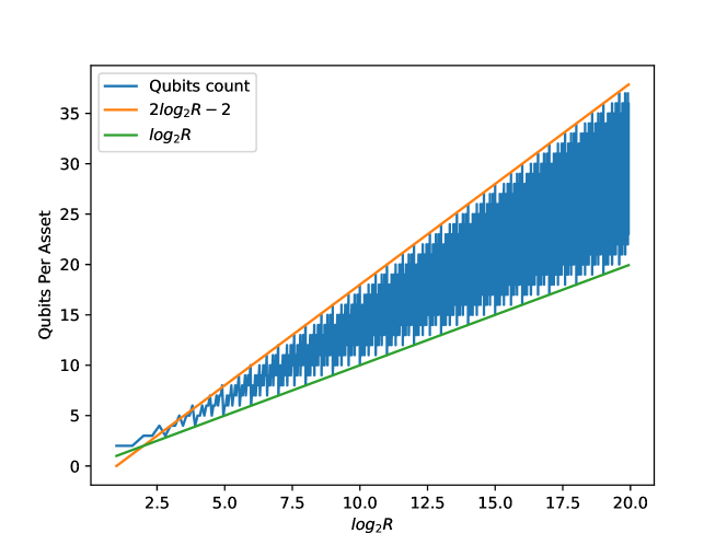
To study how the range width affects the number of qubits to encode the assets shares, we assume that all six assets have the same range, from 0 to 1. We can change the range width by adjusting the precision parameter , where . Figure 5 shows that the number of qubits for each asset is between and . For example, when ( ‰) , we need 16 qubits for each asset. By contrast, Hodson encoding needs 1000 qubits, one-hot encoding needs 1001 qubits, the binary encoding that does not support bound constraints and the Palmer encoding that is only applicable to soft constraints use 10 qubits.
4.3 Mixability
Mixability is defined as a property of a mixer that quantifies its ability to explore the feasible region of an optimization problem. A mixing operator should be able to move from one feasible quantum state to any other feasible quantum states, given suitable circuit parameters and enough layers of mixers. To quantify the performance of a mixer, we use the following metric:
| (13) |
where is the target quantum state representing the solution we want to explore, is the initial quantum state, and is the number of layers of . This equation represents the square root of the fidelity between the final state and the target state under an optimal sequence of parameters . Since and are quantum states on the computational basis, this equation also represents the modulus of the amplitude of on the final state which is a superposition state.
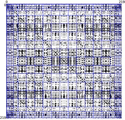
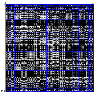
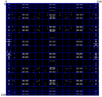
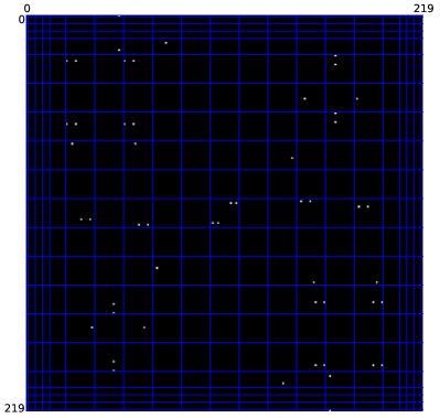
In our simulation, we focus on two stocks, NVDA and TSLA, where both the upper and lower bounds are set to 1 and -1, respectively. The precision parameter is fixed at 0.1, implying that , where . Each asset is represented by six qubits in the quasi-binary encoding, consisting of two 1-qubits, one 2-qubit, two 4-qubits, and one 8-qubit. The sum constraint is . Accordingly, the set of feasible quantum states is expressed as , where is the decoding function, is the binary sequence of the first six qubits and is the binary sequence of the last six qubits. There are 21 portfolios that satisfy the constraint, and there are 220 feasible encodings to encode these 21 portfolios under quasi-binary encoding. In Figure 6, the blue line is used to distinguish different portfolios, and pixels are used to distinguish each different encodings.
Since calculating the global optimal parameters of Equation 13 is a challenging task, we use a discrete set of points as to estimate the value of . For a parameter vector of size , we choose the parameter subject to . Then, we use the maximum value of these parameters as the estimation of Equation 13.
Figure 6 displays whether the estimation is greater than a preset threshold , when is 1, 2, 4, and 8 respectively. When the estimation of is greater than , the pixels of the row representing and the column representing are plotted as black, which means an effective conversion between and , otherwise as white. Therefore, the entire figure consists of pixels, corresponding to all 220 feasible encodings of the two assets.
By comparing the grayscale map changes under different values, we can observe that the mixability of encoding pairs that exceed the threshold is increasing. In fact, if the threshold is set to 0.0001, the entire grayscale image will become black at , which means that any two feasible quantum states will undergo effective conversion.
4.4 Real instance
In the real instance, to evaluate the performance of different algorithms to find the optimal solution, we use the approximation ratio as a metric. The approximation ratio, denoted as , is defined as
| (14) |
where and represent the costs of the optimal and worst solutions, respectively. They are obtained by the Brute-Force method. represents the average cost of all samples. For QAOA, is shown as Equation 4 or Equation 5 and for the Brute-Force method, the expectation is based on that the probability of each different solution appearing is the same.
During the parameter optimization process, we use COBYLA as the classical optimizer to find the best parameter. However, COBYLA may get trapped in different local optima depending on the initial parameter values. To overcome this challenge, we apply four different parameter scheduling methods described in Section 2.6 to determine the initial parameters.
4.4.1 Instance 1
In the first case, we select six stocks shown in Section 4.1 as the stock pool. We set , with upper and lower bounds of 1 and -1 for all assets, requiring a total of 18 qubits for the experiment. We also conduct different simulations for , , , , and , respectively.
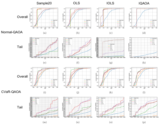
Figure 7 shows the cumulative distribution probability of the cost of each different solution under Normal-QAOA and CVaR-QAOA with four parameter estimation methods and five different depth parameters . Since the portfolio optimization problem cares more about the cumulative distribution probability of the part of the solution with the lowest cost, we separately list the cumulative distribution probability of the approximately 6.4% optimal solution as the tail.
In terms of tail performance, the CVaR-QAOA method outperforms the Normal-QAOA method significantly. The CVaR-QAOA method is superior to the Brute-force method when exceeds 2. However, under Normal-QAOA, the IOLS method needs to show its superiority at , and the IQAOA method cannot show its superiority even at . Comparing the IOLS and IQAOA methods under Normal QAOA, it can be found that these two parameter scheduling methods based on iterative methods are very easy to fall into local optimal solutions. As the value of increases, the distribution of the solutions of large and small are highly similar, but this problem does not exist in the CVaR-QAOA method. Therefore, under the quasi-binary encoding, it is recommended that the IOLS and IQAOA methods be used under the CVaR-QAOA framework. In addition, the performance at is worse than that at and in most cases. The explanation for this is that the parameter count for (32 parameters) is too large to find a better solution by classical COBYLA algorithm with 1000 iterations. However, under IOLS in Normal-QAOA method, the performance at is exceptionally good, jumping to about 52% probability at a cost of about 0.027. This also shows that once a better parameter is found at , the probability distribution of the solution is significantly improved.
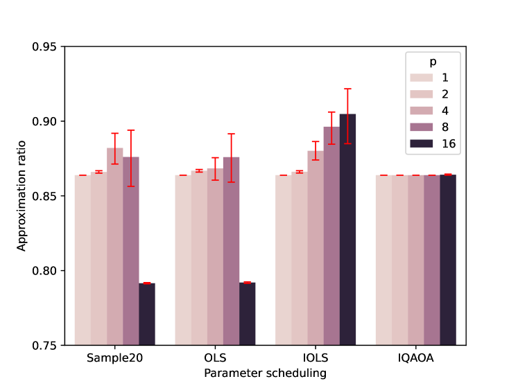
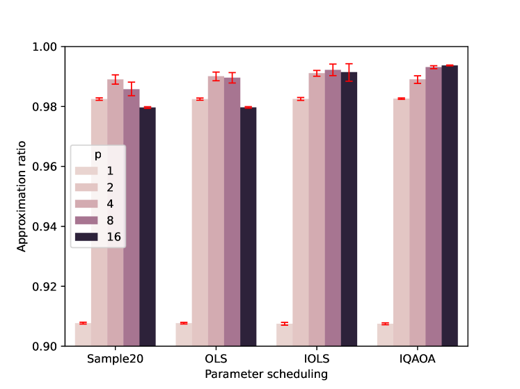
To avoid errors caused by a single experiment, we repeated the above experiment 33 times. Figures 8 and 9 show the approximation ratios of Normal-QAOA and CVaR-QAOA under different parameter scheduling methods and values, with error bars representing the 95% confidence interval. The approximation ratio of Normal-QAOA is between 0.791 and 0.905. It can also be seen that the approximation ratio decreases when under Sample20 and OLS parameter scheduling methods, and the error range is almost non-existent. This indicates that the experiment has encountered the barren plateau phenomenon at , and small-scale repetitive experiments cannot overcome this phenomenon. The approximation ratio of IOLS parameter scheduling method increases with the depth of the circuit, and the confidence interval also expands, indicating that the IOLS method can resist the barren plateau phenomenon to a certain extent. The IQAOA method shows the same behavior as shown in Figure 7, where the solution falls into a local optimum during the iterative process, and the approximation ratio remains almost unchanged from to , with little fluctuation. The approximation ratio of CVaR-QAOA ranges from 0.907 to 0.994. Among the four scheduling methods, the IQAOA method, which performs the worst under Normal-QAOA, is the best schedualing method when and . The explanation for this is that by using only the best 5% samples as the optimization target, perturbations can be added during the optimization process to overcome the problem of local optima caused by the iterative method. Therefore, we believe that in the portfolio optimization scenario, the QAOA method based on quasi-binary encoding should adopt the CVaR-QAOA estimation, and the IQAOA or IOLS parameter scheduling method. The value of is recommended to be above 8, so that the approximation ratio of the solution is above 0.99.
4.4.2 Instance 2
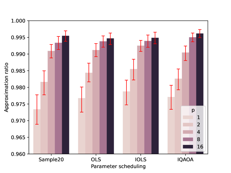
In Instance 2, we consider different stock pools and more general upper and lower bounds. The dataset for this experiment is taken from the Chinese Shenzhen and Shanghai Stock Exchange Securities Market. We randomly select 4-8 stocks from 4836 stocks in the market that do not contain unknown values. The precision is set to 0.05, and the upper and lower bounds of each stock are randomly set between 0 and 1, but the interval between the upper and lower bounds is randomly set to 0.1, 0.2, or 0.4. Then, under the quasi-binary encoding, cases with a total qubit number exceeding 20 will be excluded. We conducted 320 experiments on each combination of four parameter scheduling methods (Sample20, OLS, IOLS, IQAOA) and five different depths (=1, 2, 4, 8, 16) under the CVaR-QAOA framework. Figure 10 shows the approximation ratio in the above experiments, ranging from 0.973 to 0.997, and the error bars still represent the 95% confidence interval. In this instance, the average approximation ratio of the four parameter scheduling methods will increase as the depth increases, and the error range will become smaller. One speculation for this phenomenon is that the proportion of cases with few feasible solutions is large, and even if the COBYLA optimization algorithm falls into the barren plateau, it can still find the optimal solution in these cases. Therefore, when is large, its performance will not suffer from the barren plateau phenomenon. Among the four parameter scheduling methods, IQAOA still performs the best, consistent with the conclusion of instance 1.
5 Precision Increasing Iterative Method
Based on the simulation results of the two instances in Subsection 4.4, we observe that the precision is too coarse to meet business expectations. No asset allocation expert would accept an investment strategy with a 50% multiple as a proportion. However, if we increase the precision, for example, by setting to one-thousandth, then the total number of qubits required in Instance 1 is 96, which already exceeds the computational limit of most quantum computers and simulators.
Therefore, in this section, we propose a precision increasing iterative method where the precision parameter is exponentially reduced in each iteration, but qubits counts remain the same. The principle of this iterative method is to use QB-QAOA with a coarse precision parameter , lower bounds and upper bounds to obtain the optimal share . Then, an iteration factor is decided, and a range is generated around by radiating outward according to , resulting in new upper and lower bounds and . should be as close to the center of and as possible, and for each asset , . Next, QB-QAOA is run again with a slightly finer precision parameter to solve the portfolio optimization problem under and . In the -th iteration, the precision parameter becomes . The smaller the iteration factor is, the faster the precision parameter will be reduced, but it is also more likely to fall into local optima around previous solutions if the value of is small. It is recommended to choose such that is an integer, so that and are exactly integer multiples of . Otherwise, and need to be slightly adjusted to be divisible by . The algorithm of the iteration method is shown as Algorithm 3.
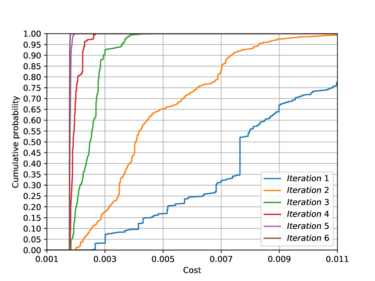
In the simulation, we utilize the experiment parameters from Instance 1 with in Section 4.4. We employ QB-QAOA with CVaR-QAOA model and IQAOA scheduling method. is set to 0.5. After six iterations, we obtained the cumulative distribution probability of solution costs of six different precisions as shown in Figure 11. It can be observed that QB-QAOA has a significant improvement in the quality of solutions under the precision increasing iterative method, and the cumulative distribution probability curve gradually converges. The worst solution in the fourth iteration is already better than the best solution in the first iteration. All six experiments used 18 qubits in the simulation.
6 Conclusion
In this paper, we have presented the quasi-binary based QAOA. This algorithm can be employed to solve combinatorial optimization problems with discrete constraint, bound constraint and sum constraint. The number of qubits allocated for each variable is logarithmically proportional to its range.
Moreover, we have proposed a precision increasing iterative method with QB-QAOA to solve portfolio optimization problems. In the course of iterative experiments with the same number of qubits, QB-QAOA has demonstrated a significant improvement in the quality of solutions.
Overall, our study has shown that QB-QAOA algorithm is a promising approach for solving portfolio optimization problems in a more efficient and effective manner. We hope that our findings will inspire further research in this area, and we believe that our proposed method can contribute to advancements in discrete quantum optimization algorithms.
Acknowledgments
I would like to express my deepest gratitude and appreciation to my colleagues at CCBFT QLab, Z.Gao, X. Zhang, H. Chen, D. Yu, and H. Hou. Their valuable insights and contributions have been essential to the success of this project. I would also like to extend my sincere thanks to Q. Zhang, Z. Wang, and N. Qu at China Construction Bank Group Fintech Innovation Center for their help in verifying the phase separation Hamiltonian formulae and deriving the risk factors. Last but not least, I would like to thank K. Feng from Pengpai News for her assistance in designing the multiple images used in this paper. Without the contributions and support of these individuals, this paper would not have been possible. Thank you all once again for your invaluable assistance.
Funding
This work was supported by CCB Fintech Company Limited (No. PO3522083587, No. PO3522083675) and by Chengdu Science and Technology Bureau (No. 2021-YF09-00114-GX).
Conflicts of Interest
The authors have declared that there is no conflict of interest regarding the publication of this article.
Data Availability
The original data analyzed in this research article were the closing prices of six well-known NASDAQ companies (Apple/Amazon/Google/Microsoft/NVIDIA/Tesla) during the period of 2022.12.02 to 2023.02.28. The data were obtained from Yahoo Finance, such as for Tesla company, the data were obtained from https://finance.yahoo.com/quote/TSLA/history?p=TSLA. The data are openly available and can be accessed freely without any restrictions from the source. The data of the Chinese stock market in Instance 2 is sourced from the stock data of the Shanghai and Shenzhen exchanges from May 4th, 2023 to August 8th, 2023, which is accessed by the open-source software package QStock.
Ethics approval
This study doesn not include human or animal subjects.
Author contributions
All authors contributed to the study conception and design. The first draft of the manuscript was written by Bingren Chen. The numerical simulation, the new discrete model and iterative method are presented by Bingren Chen. The construction of the quasi-binary encoding and the XYY-mixer are presented by Hanqing Wu. All authors commented on previous versions of the manuscript. All authors read and approved the final manuscript.
References
- [1] Richard P. Feynman. Quantum Mechanical Computers. Optics News, 11(2):11–20, February 1985. Publisher: Optica Publishing Group.
- [2] Maria Schuld, Ilya Sinayskiy, and Francesco Petruccione. An introduction to quantum machine learning. Contemporary Physics, 56(2):172–185, April 2015.
- [3] Miloslav Dušek, Norbert Lütkenhaus, and Martin Hendrych. Quantum cryptography. Progress in optics, 49:381–454, 2006. Publisher: Elsevier Amsterdam.
- [4] Yudong Cao, Jonathan Romero, Jonathan P. Olson, Matthias Degroote, Peter D. Johnson, Mária Kieferová, Ian D. Kivlichan, Tim Menke, Borja Peropadre, Nicolas P. D. Sawaya, Sukin Sim, Libor Veis, and Alán Aspuru-Guzik. Quantum Chemistry in the Age of Quantum Computing. Chemical Reviews, 119(19):10856–10915, October 2019.
- [5] Ira N. Levine, Daryle H. Busch, and Harrison Shull. Quantum chemistry, volume 6. Pearson Prentice Hall Upper Saddle River, NJ, 2009.
- [6] Neill Lambert, Yueh-Nan Chen, Yuan-Chung Cheng, Che-Ming Li, Guang-Yin Chen, and Franco Nori. Quantum biology. Nature Physics, 9(1):10–18, 2013. Publisher: Nature Publishing Group UK London.
- [7] Edward Farhi, Jeffrey Goldstone, and Sam Gutmann. A Quantum Approximate Optimization Algorithm. arXiv: [quant-ph], November 2014.
- [8] Jules Tilly, Hongxiang Chen, Shuxiang Cao, Dario Picozzi, Kanav Setia, Ying Li, Edward Grant, Leonard Wossnig, Ivan Rungger, and George H. Booth. The variational quantum eigensolver: a review of methods and best practices. Physics Reports, 986:1–128, 2022. Publisher: Elsevier.
- [9] A. B. Finnila, M. A. Gomez, C. Sebenik, C. Stenson, and J. D. Doll. Quantum annealing: A new method for minimizing multidimensional functions. Chemical Physics Letters, 219(5):343–348, 1994.
- [10] Stuart Hadfield, Zhihui Wang, Bryan O’Gorman, Eleanor G. Rieffel, Davide Venturelli, and Rupak Biswas. From the Quantum Approximate Optimization Algorithm to a Quantum Alternating Operator Ansatz. Algorithms, 12(2):34, February 2019.
- [11] Junde Li, Mahabubul Alam, and Swaroop Ghosh. Large-scale quantum approximate optimization via divide-and-conquer. IEEE Transactions on Computer-Aided Design of Integrated Circuits and Systems, 2022. Publisher: IEEE.
- [12] Mark Hodson, Brendan Ruck, Hugh Ong, David Garvin, and Stefan Dulman. Portfolio rebalancing experiments using the Quantum Alternating Operator Ansatz, November 2019.
- [13] Zhihui Wang, Nicholas C. Rubin, Jason M. Dominy, and Eleanor G. Rieffel. XY-mixers: Analytical and numerical results for QAOA. Physical Review A, 101(1):012320, January 2020.
- [14] Pradeep Niroula, Ruslan Shaydulin, Romina Yalovetzky, Pierre Minssen, Dylan Herman, Shaohan Hu, and Marco Pistoia. Constrained quantum optimization for extractive summarization on a trapped-ion quantum computer. Scientific Reports, 12(1):17171, October 2022. Number: 1 Publisher: Nature Publishing Group.
- [15] N. Slate, E. Matwiejew, S. Marsh, and J. B. Wang. Quantum walk-based portfolio optimisation. Quantum, 5:513, July 2021.
- [16] Xinyu Ye, Ge Yan, and Junchi Yan. Towards Quantum Machine Learning for Constrained Combinatorial Optimization: a Quantum QAP Solver. In Proceedings of the 40th International Conference on Machine Learning, pages 39903–39912. PMLR, July 2023. ISSN: 2640-3498.
- [17] Samuel Palmer, Serkan Sahin, Rodrigo Hernandez, Samuel Mugel, and Roman Orus. Quantum Portfolio Optimization with Investment Bands and Target Volatility, August 2021. arXiv:2106.06735 [quant-ph, q-fin].
- [18] Andreas Bärtschi and Stephan Eidenbenz. Grover Mixers for QAOA: Shifting Complexity from Mixer Design to State Preparation. In 2020 IEEE International Conference on Quantum Computing and Engineering (QCE), pages 72–82, October 2020.
- [19] Franz Georg Fuchs, Kjetil Olsen Lye, Halvor Møll Nilsen, Alexander Johannes Stasik, and Giorgio Sartor. Constraint Preserving Mixers for the Quantum Approximate Optimization Algorithm. Algorithms, 15(6):202, June 2022.
- [20] Tianyi Hao, Ruslan Shaydulin, Marco Pistoia, and Jeffrey Larson. Exploiting In-Constraint Energy in Constrained Variational Quantum Optimization. In 2022 IEEE/ACM Third International Workshop on Quantum Computing Software (QCS), pages 100–106, Dallas, TX, USA, November 2022. IEEE.
- [21] Sebastian Brandhofer, Daniel Braun, Vanessa Dehn, Gerhard Hellstern, Matthias Hüls, Yanjun Ji, Ilia Polian, Amandeep Singh Bhatia, and Thomas Wellens. Benchmarking the performance of portfolio optimization with QAOA. Quantum Information Processing, 22(1):25, December 2022.
- [22] Dylan Herman, Ruslan Shaydulin, Yue Sun, Shouvanik Chakrabarti, Shaohan Hu, Pierre Minssen, Arthur Rattew, Romina Yalovetzky, and Marco Pistoia. Constrained optimization via quantum Zeno dynamics. Communications Physics, 6(1):1–17, August 2023. Number: 1 Publisher: Nature Publishing Group.
- [23] Harry M. Markowitz. Foundations of portfolio theory. The journal of finance, 46(2):469–477, 1991.
- [24] Panagiotis Kl Barkoutsos, Giacomo Nannicini, Anton Robert, Ivano Tavernelli, and Stefan Woerner. Improving Variational Quantum Optimization using CVaR. Quantum, 4:256, April 2020.
- [25] Nicholas Chancellor. Domain wall encoding of discrete variables for quantum annealing and QAOA. Quantum Science and Technology, 4(4):045004, October 2019.
- [26] Daniel J. Egger, Jakub Mareček, and Stefan Woerner. Warm-starting quantum optimization. Quantum, 5:479, June 2021.
- [27] Reuben Tate, Majid Farhadi, Creston Herold, Greg Mohler, and Swati Gupta. Bridging Classical and Quantum with SDP initialized warm-starts for QAOA. ACM Transactions on Quantum Computing, 4(2):9:1–9:39, February 2023.
- [28] Wim van Dam, Karim Eldefrawy, Nicholas Genise, and Natalie Parham. Quantum Optimization Heuristics with an Application to Knapsack Problems. arXiv: [quant-ph], October 2021.
- [29] Salvatore Certo, Anh Dung Pham, and Daniel Beaulieu. Comparing Classical-Quantum Portfolio Optimization with Enhanced Constraints, March 2022.
- [30] Samuel Fernández-Lorenzo, Diego Porras, and Juan José García-Ripoll. Hybrid quantum–classical optimization with cardinality constraints and applications to finance. Quantum Science and Technology, 6(3):034010, June 2021.
- [31] Shree Hari Sureshbabu, Dylan Herman, Ruslan Shaydulin, Joao Basso, Shouvanik Chakrabarti, Yue Sun, and Marco Pistoia. Parameter Setting in Quantum Approximate Optimization of Weighted Problems, January 2024. arXiv:2305.15201 [quant-ph].
- [32] James D. Whitfield, Jacob Biamonte, and Alán Aspuru-Guzik. Simulation of electronic structure Hamiltonians using quantum computers. Molecular Physics, 109(5):735–750, March 2011.
- [33] Yordan S. Yordanov, David R. M. Arvidsson-Shukur, and Crispin H. W. Barnes. Efficient quantum circuits for quantum computational chemistry. Physical Review A, 102(6):062612, December 2020.
- [34] Edward Farhi, Jeffrey Goldstone, Sam Gutmann, and Leo Zhou. The Quantum Approximate Optimization Algorithm and the Sherrington-Kirkpatrick Model at Infinite Size. Quantum, 6:759, July 2022. Publisher: Verein zur Förderung des Open Access Publizierens in den Quantenwissenschaften.
- [35] M. J. D. Powell. A Direct Search Optimization Method That Models the Objective and Constraint Functions by Linear Interpolation. In Susana Gomez and Jean-Pierre Hennart, editors, Advances in Optimization and Numerical Analysis, Mathematics and Its Applications, pages 51–67. Springer Netherlands, Dordrecht, 1994.
- [36] M. J. D. Powell. Direct search algorithms for optimization calculations. Acta Numerica, 7:287–336, January 1998. Publisher: Cambridge University Press.
- [37] Michael JD Powell. The BOBYQA algorithm for bound constrained optimization without derivatives. Cambridge NA Report NA2009/06, University of Cambridge, Cambridge, 26, 2009.
- [38] Stefan H. Sack and Maksym Serbyn. Quantum annealing initialization of the quantum approximate optimization algorithm. quantum, 5:491, 2021. Publisher: Verein zur Förderung des Open Access Publizierens in den Quantenwissenschaften.
- [39] Michael Streif and Martin Leib. Training the quantum approximate optimization algorithm without access to a quantum processing unit. Quantum Science and Technology, 5(3):034008, 2020. Publisher: IOP Publishing.
- [40] Matija Medvidović and Giuseppe Carleo. Classical variational simulation of the quantum approximate optimization algorithm. npj Quantum Information, 7(1):101, 2021. Publisher: Nature Publishing Group UK London.
- [41] Ruslan Shaydulin and Stefan M. Wild. Exploiting Symmetry Reduces the Cost of Training QAOA. IEEE Transactions on Quantum Engineering, 2:1–9, 2021.
- [42] Ruslan Shaydulin and Yuri Alexeev. Evaluating quantum approximate optimization algorithm: A case study. In 2019 tenth international green and sustainable computing conference (IGSC), pages 1–6. IEEE, 2019.
- [43] Lennart Bittel and Martin Kliesch. Training Variational Quantum Algorithms Is NP-Hard. Physical Review Letters, 127(12):120502, September 2021.
- [44] Ruslan Shaydulin, Ilya Safro, and Jeffrey Larson. Multistart methods for quantum approximate optimization. In 2019 IEEE high performance extreme computing conference (HPEC), pages 1–8. IEEE, 2019.
- [45] Phillip C. Lotshaw, Travis S. Humble, Rebekah Herrman, James Ostrowski, and George Siopsis. Empirical performance bounds for quantum approximate optimization. Quantum Information Processing, 20(12):403, December 2021.
- [46] Alexey Galda, Xiaoyuan Liu, Danylo Lykov, Yuri Alexeev, and Ilya Safro. Transferability of optimal QAOA parameters between random graphs. In 2021 IEEE International Conference on Quantum Computing and Engineering (QCE), pages 171–180, October 2021.
- [47] Ruslan Shaydulin, Phillip C. Lotshaw, Jeffrey Larson, James Ostrowski, and Travis S. Humble. Parameter Transfer for Quantum Approximate Optimization of Weighted MaxCut. ACM Transactions on Quantum Computing, 4(3):1–15, September 2023.
- [48] Ruslan Shaydulin, Stuart Hadfield, Tad Hogg, and Ilya Safro. Classical symmetries and the Quantum Approximate Optimization Algorithm. Quantum Information Processing, 20(11):359, October 2021.
Appendix A Markowitz model
The Markowitz model serves the purpose of determining the proportion of funds to be invested in each asset out of the total funds, given the covariance matrix and expected returns of assets. The original Markowitz model is expressed by the following equation:
| (A) | ||||
Here, represents the vector of investment proportions for the assets, denotes the minimum target return, is the covariance matrix of returns, is the vector of returns expectation, and represents a vector of ones.
Upon performing some transformations, the Markowitz model can be expressed in an equivalent form as follows:
| (B) | ||||
where represents the risk factor, where higher values indicate a more conservative investment strategy that places greater emphasis on risk, and lower values indicate a more aggressive strategy that prioritizes returns. The relationship between and is given by:
| (C) |
where the constants , , and are defined as:
| (D) | ||||
Figure 12 illustrates the efficient frontier of the Markowitz model. The depicted scatter points correspond to Eq. A, which represents the values of for different investment portfolios under the constraints of and . The straight line in the graph corresponds to Eq. B, which takes the form of or , where indicates the intersection of the line with the y-axis.
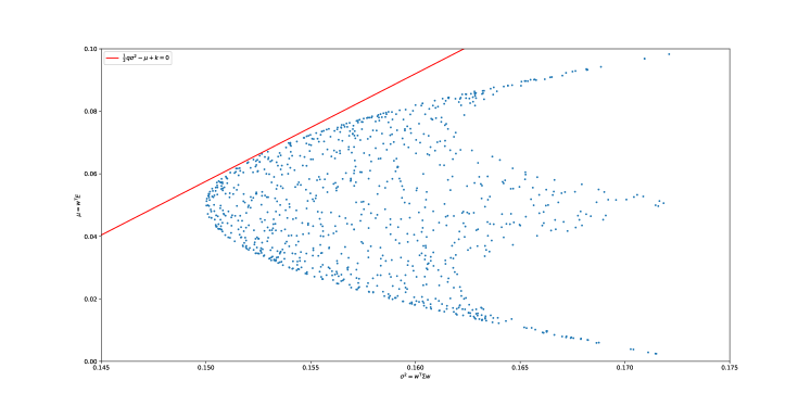
It is worth noting that the upper boundary of the scatter points forms a curve that satisfies the constraints of and . By solving for and substituting it into , we obtain the equation of the efficient frontier curve as:
| (E) |
where the values of , , and are presented in Eq. D.
We should expect that the optimal solutions obtained from Eq. A and Eq. B would coincide with each other. Therefore, the optimal expectation and risk should satisfy both the equation of the straight line and the equation of the curve.
Now, we calculate the partial derivative of Eq. E with respect to , yielding:
| (F) |
The value of Eq. F should be equal to the slope of the straight line, which is . Hence, by solving:
| (G) |