Iron-Peak Element Abundances in Warm Very Metal-Poor Stars

Abstract

We have derived new detailed abundances of Mg, Ca, and the Fe-group elements Sc through Zn (Z = 21$-$30) for 37 main sequence turnoff very metal-poor stars ([Fe/H] $\lesssim$ $-$2.1). We analyzed Keck HIRES optical and near-UV high signal-to-noise spectra originally gathered for a beryllium abundance survey. Using typically $\sim$400 Fe-group lines with accurate laboratory transition probabilities for each star, we have determined accurate LTE metallicities and abundance ratios for neutral and ionized species of the 10 Fe-group elements as well as $\alpha$ elements Mg and Ca. We find good neutral/ion abundance agreement for the 6 elements that have detectable transitions of both species in our stars in the 3100$-$5800 Å range. Earlier reports of correlated Sc-Ti-V relative overabundances are confirmed, and appear to slowly increase with decreasing metallicity. To this element trio we add Zn; it also appears to be increasingly overabundant in the lowest metallicity regimes. Co appears to mimic the behavior of Zn, but issues surrounding its abundance reliability cloud its interpretation.

1 INTRODUCTION

Almost all elements in the Universe are formed in stars. Elemental abundances in very low metallicity stars, among the oldest in the Galaxy and the Universe, provide important clues to early Galactic nucleosynthesis. Such observed abundances provide insight into the identities of the very first stars (long-since gone) and the nature of the nuclear processes that occurred in those stars (e.g., Curtis et al. 2019, Ebinger et al. 2020, Cowan et al. 2021). These processes can occur in environments typical of supernovae (SNe) in core-collapse explosions from massive stars, or Type Ia explosions resulting from binary interactions. Comparisons between the low metallicity stars and more metal-rich groups indicate changes in chemical evolution over time pointing to variations in stellar mass ranges and synthesis mechanisms over Galactic timescales. Such comparisons, however, require accurate abundance determinations, which in turn depend sensitively upon precise experimental atomic physics data and high-resolution, high signal-to-noise ratio (SNR) astronomical spectra.

Our earlier work in this area focused on the neutron-capture, particularly Rare Earth, elemental abundances in stars. Those efforts involved obtaining large amounts of experimental atomic data (line transition probabilities and isotopic/hyperfine sub-component parameters) from the Wisconsin physics group. These new experimental data, applied to ground-based and space-based stellar spectra, led to precise elemental abundances of a large number of neutron-capture elements in metal-poor stars (e.g., Lawler et al. 2009, Sneden et al. 2009, Holmbeck et al. 2018, Roederer et al. 2022 and references therein).

More recently we have concentrated on iron-group elements, Z = 21$-$30 (see Sneden et al. 2016, Lawler et al. 2017, Wood et al. 2018, Lawler et al. 2018, Lawler et al. 2019, Den Hartog et al. 2019, Cowan et al. 2020). Many of these studies used the bright well-known metal-poor ([Fe/H] $\sim$ $-$2.2) main sequence turnoff star HD 84937, which has well-known atmospheric parameters and large amounts of high-resolution spectroscopic data. In Cowan et al. Fe-group abundances were determined in 3 main-sequence turnoff stars ([Fe/H] $\sim$ $-$3) with HST/STIS vacuum-$UV$ (2300$-$3050 Å) high resolution spectra. In that study we were able to derive abundances from both neutral and ionized species for 6 out of the 10 Fe-group elements.

Unfortunately, only a few very metal-poor stars have vacuum $UV$ high resolution spectra, and that number is unlikely to grow much in the future. From basic atomic structure considerations, for most metallic species the number of transitions and their strengths rise rapidly with decreasing wavelength (e.g., Figure 2 in Lawler et al. 2017 and other examples in our laboratory transition paper series). Therefore, many of the Fe-group species best studied in the vacuum-$UV$ also have large numbers of transitions available in the near-$UV$, $\lambda\lambda$3000$-$4000 Å. Boesgaard et al. (2011) (hereafter called B11) derived Be and alpha element abundances for 117 main-sequence stars in the disk and halo ($-$3.5 $\leq$ [Fe/H] $\leq$ $-$0.5). For Be they studied the Be ii resonance doublet at 3130.4, 3131.1 Å. Gathering high SNR spectra at these wavelengths ensured that we could study Fe-group transitions nearly to the atmospheric ozone cutoff.

Here we present new abundances of Fe-group elements in 37 very metal-poor main sequence turnoff stars ([Fe/H] $\leq$ $-$2.0), from our analyses of B11 Keck HIRES spectra. In §2 we introduce the high-resolution spectroscopic data set, followed by the abundance analysis in §3. Interpretation of the abundance trends is given in §4. Finally, a summary and conclusions are detailed in §5.

2 SPECTROSCOPIC DATA

The B11 Be abundance survey required high SNR data near 3100 Å. This spectral region suffers significant telluric extinction, so only relatively $UV$-bright metal-poor stars were available for the Boesgaard et al. study. This restriction generally ruled out metal-poor red giants, which have steeply declining fluxes in the near-$UV$. Additionally, the deep atmospheres of red giants produce very strong-lined spectra even for metallicities [Fe/H] $<$ $-$2, rendering abundance analyses in the near-$UV$ very difficult. Therefore the B11 sample was limited to warm main sequence turnoff and subgiant stars: 5500 K $\lesssim$ T_eff $\lesssim$ 6500 K, and 3.0  $\lesssim$ log g $\lesssim$ 4.8.

The spectra were all obtained with Keck I/HIRES (Vogt et al., 1994), which yielded spectral resolving power $R$ $\equiv$ $\lambda/\Delta\lambda$ $\simeq$ 42,000 in the near-$UV$. These echelle spectra have near-continuous wavelength coverage in the interval 3050 Å $\lesssim$ $\lambda$ $\lesssim$ 5900 Å. For the complete data set B11 estimated the signal-to-noise to be $\langle$SNR$\rangle$ = 106 at 3130 Å. The $SNR$ increases rapidly toward longer wavelengths, typically exceeding values of 200 near 4000 Å and 300 near 5000 Å. The $SNR$ ratio is not an issue in our abundance analyses.

A more significant concern is the natural complexity of the program star near-$UV$ spectra at high metallicities. In Figure 1 we show a small near-$UV$ wavelength region of interest to this investigation. Note especially in this figure the two Cu i resonance lines, detectable even in the lowest metallicity stars. Four stars with metallicities increasing by about a factor of 10 each step from top to bottom in the figure are displayed. Inspection of these spectra suggests that while continuum points can be easily established for stars with [Fe/H] $\lesssim$ $-$2.0, this determination becomes challenging by [Fe/H] $\gtrsim$ $-$1.5 and practically impossible for [Fe/H] $\gtrsim$ $-$1.0.

Our astrophysical goal was to investigate the relative abundances of Fe-group elements in very metal-poor stars, using very large numbers of neutral and ionized lines with recent laboratory transition data. To accomplish this task for many stars, examining each transition for its abundance utility in each star, we used equivalent width ($EW$) measurements instead of synthetic/observed spectrum matches. The near-UV absorption line crowding displayed in the higher metallicity stars of Figure 1 left relatively few unblended spectral features in them for analysis. Therefore we limited our program star list to the B11 stars with [Fe/H] $\lesssim$ $-$2.1, adding one star with [Fe/H] $\simeq$ $-$1.4 to test our analytical methods in a higher metallicity regime.

Final reduction steps were accomplished with IRAF software (Tody, 1986, 1993), including clipping of radiation events with task $lineclean$ and concatenation of spectral orders with task $scombine$. Then the spectra were divided into 100 Å segments. These spectrum pieces were subjected to detailed continuum normalization with spline functions in the specialized software package $SPECTRE$ (Fitzpatrick & Sneden, 1987), as well as smoothing with 2-pixel Gaussian functions.

3 ABUNDANCE ANALYSIS

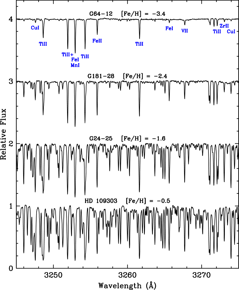
Figure 1: Sample Keck I/HIRES spectra of four stars from the B11 survey. This small region illustrates the near-UV line density in main sequence turnoff stars of different metallicities. Stars G64-12 and G181-28 are part of the present study, while stars G24-25 and HD 109303 are too “metal-rich” to be included here. The metallicities quoted in the figure legend are from B11 Table 2. The relative flux scale is correct for HD 109303, and the other spectra have been shifted successively by additive constants of 1.0 for display purposes. Major absorption features have been identified for the G64-12 spectrum.

All abundance computations were performed with the current version of the plane-parallel LTE line analysis code MOOG (Sneden, 1973). The program stars are all warm, high gravity stars, with continuum opacities dominated by H^- even at the near-$UV$ wavelengths of this study. Therefore no special computations (Sobeck et al., 2011) were required to account for continuum Rayleigh scattering, which we confirmed with abundance tests.

We employed more than about 350 Fe-group lines for each program star, which made synthetic spectrum analyses impractical, as discussed in §2. We relied almost exclusively on $EW$ measurements, which limited the line lists to relatively unblended transitions with nearby well-defined continuum points. We used $SPECTRE$ for semi-automated $EW$ measurements, with visual inspection of each line profile. This procedure allowed for elimination of very weak lines and those with distorted profiles, and for re-measurement of very strong lines that display obvious Voigt profile wings. In the weak-line domain we usually discarded lines with reduced widths log $RW$ $\equiv$ log($EW$/$\lambda$) $\lesssim$ $-$6.3 ($EW$ $\sim$ 2 mÅ at 4000 Å) and only retained lines with log $RW$ $<$ $-$6.0 if their line profiles were clean and not affected by continuum noise fluctuations. For strong lines we discarded lines with log $RW$ $\gtrsim$ -4.5 ($EW$ $\sim$125 mÅ at 4000 Å). Lines stronger than this limit are on the damping part of the curve-of-growth. Abundances derived from them depend strongly on microturbulent velocity and damping parameters. Our $EW$s are available in the Zenodo database.

3.1 Atomic Transitions

Discussions of line selection and laboratory data have appeared in Sneden et al. (2016), and Cowan et al. (2020), often with comments on the laboratory studies that will be cited here on individual Fe-group species. Only lines from these papers are employed in our study. Data for these transitions may be found in the $linemake$ on-line facility (Placco et al., 2021).

Most lines were assumed to be single transitions, but those of odd-Z elements Sc, V, Mn, Co, and Cu have significant hyperfine substructure (hfs) that can significantly broaden spectral features, leading to desaturation and consequent decrease in derived abundances from strong lines. The hfs substructures are especially large for Co i, with abundance corrections reaching $\sim$0.5 dex for the strongest transitions. For all lines that have known hfs patterns and are strong enough to have any possibility of saturation ($RW$ $>$ $-$5.5), we derived abundances with $MOOG$’s $EW$ option blends. Here we briefly summarize the lines used in our computations. Issues arising in the abundance computations will be discussed in §3.3.

Magnesium: There are no recent comprehensive transition probability studies of Mg i lines, but generally they are well-determined from past atomic physics studies. The NIST Atomic Spectra Database (NIST ASD, Kramida et al. 2022) gives quality ratings of “B” ($<\pm$10% uncertainty) for all lines of interest here, except for 4571.10 Å(rating D, $<\pm$50% uncertainty). None of the Mg abundances in our study were determined only from the $\lambda$4571 line.

Calcium: This element was not considered in our earlier papers due to the lack of recent laboratory work. A new study by Den Hartog et al. (2021) has derived transition probabilities for Ca i, and we have adopted log($gf$) values from that work. A few Ca ii lines that are weak enough for abundance analyses appear in our spectra, notably those at $\lambda\lambda$3158.87, 3179.33, and 3706.03. Den Hartog et al. showed that abundances from Ca ii lines using transition probabilities from Safronova & Safronova (2011) were in agreement with Ca i values for one metal-poor main sequence star, HD 84937. We included these Ca ii transitions in the present study.

Scandium: Laboratory transition probabilities and hfs patterns for Sc ii were taken from Lawler et al. (2019). No Sc i lines are strong enough for detection in metal-poor stars. Hyperfine substructure does affect Sc ii and lowers the derived Sc abundances, but the effect is modest for our stars, typically $\lesssim$0.03 dex

Titanium: Neutral and ionized species of Ti have many available transitions in our spectra. Their lab data were taken from Lawler et al. (2013) and Wood et al. (2013).

Vanadium: Our abundances were mostly based on numerous transitions of V ii. In a few stars a handful of extremely weak V i lines can be detected. The transition data were adopted from Lawler et al. (2014) and Wood et al. (2014a). Full hfs calculations were necessary for the V ii transitions.

Chromium: The laboratory transition data for Cr i and Cr ii were taken from Sobeck et al. (2007) and Lawler et al. (2017), respectively. Our abundances were determined from large line samples, on average 8 for Cr i and 16 for Cr ii. This permitted us to explore the known disagreement between Cr abundances derived from neutral and ionized species (e.g., Kobayashi et al. 2006, Sobeck et al. 2007, Roederer et al. 2014).

Manganese: Transition probabilities and hfs components for both Mn i and Mn ii were taken from Den Hartog et al. (2011). Only about 5 lines each are available for neutral and ionized Mn species. For Mn i often the derived abundances were based entirely on the resonance triplet at 4030.76, 4033.07, and 4034.49 Å. This set of lines has been responsible for most Mn abundance results in the literature of very metal-poor stars, and is known to yield much lower abundances than other neutral and ionized Mn lines. We will discuss this issue in §3.3.

Iron: As in Cowan et al. (2020), we limited our Fe i transition set to those published in the collaborative laboratory effort of the Imperial College London and the University of Wisconsin atomic physics groups: Ruffoni et al. (2014), Den Hartog et al. (2014), Belmonte et al. (2017). Recently Den Hartog et al. (2019) determined new transition probabilities for Fe ii. Most of that laboratory effort concentrated on the very strong lines in the vacuum UV, and the $gf$ values at longer wavelengths combined new branching fractions and previous lifetime measurements. See Den Hartog et al. (2019) Cowan et al. (2020) for further comments on this issue.

Cobalt: Both Co i and Co ii have recent lab transition probability and hfs analyses (Lawler et al. 2015, Lawler et al. 2018). However, Co ii has strong transitions only in the vacuum $UV$ ($\lambda$ $<$ 3050 Å). Lawler et al. (2018) report lab $gf$ values for six lines in the 3300$-$3600 Å spectral region. Unfortunately they all are very weak in our program stars, and most of them are severely blended with transitions of other species. In the solar spectrum, the relatively unblended Co ii lines have $EW$ $\lesssim$ 30 mÅ (Moore et al., 1966). In our metal-poor program stars their maximum $EW$ values should be no more than a few mÅ. We verified their absence in each of our stars.

Nickel: Ni abundances were derived exclusively from Ni i transitions, with laboratory data taken from Wood et al. (2014b). All potentially detectable Ni ii lines occur in the vacuum $UV$, inaccessible for this study. Cowan et al. (2020) had HST/STIS data for their small sample of turnoff stars with [Fe/H] $\sim$ $-$3, and the two Ni species yielded consistent abundances, suggesting that the Ni i lines used here can be trusted to yield reliable elemental abundances.

Figure 2: Abundances from individual Fe i and Fe ii lines (blue and red points, respectively) in the program star LP 815-43. The three panels show these abundances as functions of excitation energy $\chi$, reduced width $RW$, and wavelength. In each panel the dashed line represents the mean abundance from Fe i, and the dotted lines represent the sample standard deviations $\sigma$. The Fe abundances are those derived with a model atmosphere with T_eff = 6350 K, log g = 4.00, $\xi_{\rm t}$ = 1.30 km s^-1, and model metallicity [Fe/H] = $-$2.9.

Copper: The atomic structure of this element gives rise only to a few Cu i lines; Cu ii has no detectable lines in the optical spectral region. Usually the Cu i resonance lines at 3247.5 and 3273.9 Å were the only detectable transitions, with the 5105.5 Å line available on rare occasions. There are no recent lab studies of this species, but the transition probabilities of the resonance lines are of high accuracy: the NIST database rates them as “AA” ($\leq$1% uncertainty). Abundance computations including hfs were performed for these lines using the $gf$ values recommended in the NIST ASD (Kramida et al., 2019) website.

Zinc: We could only detect the Zn i near-UV high-excitation lines at 3302.6, 3345.0 Å to supplement the optical lines at 4722.16 and 4810.54 Å that have been employed in nearly all previous studies in metal-poor stars. All of these lines are extremely weak, and abundances were derived for them from both $EW$ and synthetic spectrum analyses. The near-UV lines have multiple components. Each of them has one strong member; the weaker components are split redward by $\gtrsim$0.4 Å and are blended and barely detectable in our spectra.

3.2 Model Atmospheres

Initial model atmospheric parameters T_eff, log g, [Fe/H] metallicity, and $\xi_{\rm t}$ were taken from Table 2 of B11. These values were used to generate interpolated models from the Kurucz (2011, 2018) alpha-enhanced model grid using software kindly provided by Andrew McWilliam and Inese Ivans.

We determined abundances with these models and assessed the assumed model parameters with standard criteria: for T_eff, that there be no significant abundance differences between low and high excitation lines of Fe i; for $\xi_{\rm t}$, that there be no differences between weak and strong lines for Fe i and Ni i; for log g, that the mean neutral and ionized abundances of Ca, Ti, and Fe agree; and for metallicity, that the model [Fe/H] was similar to the derived [Fe/H]. In comparing abundances from weak and strong lines, from low and high excitation lines, and from neutral and ionized lines the mean abundance differences were held to less than 0.10 dex whenever possible. In Figure 2 we show a typical example of this process applied to the neutral and ionized Fe lines.

In Table 1 we list the derived model parameters and metallicities determined from both Fe i and Fe ii transitions. In general our new parameters are close to those derived by B11. Defining $\Delta$A $\equiv$ A${}_{this~{}work}$ $-$ A_B11, for any parameter A, we found $\langle\Delta$T_eff$\rangle$ = 80 $\pm$ 23 K ($\sigma$ = 137 K); $\langle\Delta$log g$\rangle$ = $-$0.05 $\pm$ 0.05 ($\sigma$ = 0.33); $\langle\Delta$$\xi_{\rm t}$$\rangle$ = $-$0.15 $\pm$ 0.02 km s^-1 ($\sigma$ = 0.14 km s^-1); and $\langle\Delta$[Fe/H]$\rangle$ = $-$0.10 $\pm$ 0.02 ($\sigma$ = 0.13).

Only one star merits comment in this atmospheric parameter comparison, BD $-$10 388. Our analysis of this star yielded somewhat different values compared to B11. Our parameters (T_eff,log g, [Fe/H]) = (6350,4.00,$-$2.43) put BD $-$10 388 essentially at the main sequence turnoff, while the B11 parameters (5768 K,3.04,$-$2.79) suggest subgiant status. Other studies yield mixed parameters, e.g., (6009,4.14,$-$2.33, Reddy & Lambert 2008), or (5931,3.77,$-$2.62, Bensby & Lind 2018). The Gaia photometric-based parameters (Gaia Collaboration et al., 2016, 2022) (6275,4.05,$-$2.22)) are in good agreement with our values. BD $-$10 388 deserves further investigation in the future, but excluding it from our comparison with B11 yields little change in the mean results and smaller scatter: $\langle\Delta$T_eff$\rangle$ = 66 $\pm$ 18 K ($\sigma$ = 109 K); $\langle\Delta$log g$\rangle$ = $-$0.07 $\pm$ 0.05 ($\sigma$ = 0.28); $\langle\Delta$($\xi_{\rm t}$$\rangle$ = $-$0.16 $\pm$ 0.02 km s^-1 ($\sigma$ = 0.14 km s^-1); and $\langle\Delta$[Fe/H]$\rangle$ = $-$0.11 $\pm$ 0.02 ($\sigma$ = 0.10).

3.3 Abundances

Figure 3: Elemental abundance ratios [X/Fe] as functions of [Fe/H] metallicity for light elements Mg, Ca, and the 3 lightest Fe-group elements Sc, Ti, and V. Blue colors, lines and open circles are for neutral-species transitions, while red and X-symbols are for ionized species transitions. Vertical bars in the lower corners indicate the mean line-to-line abundance scatters for individual abundances. The quoted statistics refer to the mean [X/Fe] value for a species for all stars, and $\sigma$ is its sample deviation.

Figure 4: Elemental abundance ratios [X/Fe] as functions of [Fe/H] metallicity for heavier Fe-group elements Cr, Mn, Co, Ni, Cu, and Zn. Colors, symbols, and lines are as in Figure 3.

Figure 5: Abundance differences between derived neutral and ionized abundances for Cr (top panel) and Mn (bottom panel). As noted in the panel legends, the dark green open circles are for the differences if all neutral lines are considered, while the purple filled circles are for differences that include only excited-state lines, $\chi$ $>$ 0.0 eV. The black dashed lines are for perfect agreement between the two species. The dotted lines indicate the mean differences including all stars.

Abundance computations were straightforward applications of the model atmospheres described in §3.2 with the model parameters of Table 1 to the measured $EW$s. For even-Z elements the transitions were treated as single lines using the $abfind$ option in $MOOG$. For odd-Z elements the line hfs components were accounted for in option $blends$. Table 2 contains all abundances for all stars in [X/Fe] form, where these values have been computed with like ionization states, that is neutral species compared to Fe i and ionized species compared to Fe ii. These abundance ratios are displayed as functions of metallicity in Figures 3 and 4. Inspection of these figures suggests that for most elements the star-to-star [X/Fe] scatter is small at most metallicities, and mean [X/Fe] values generally are constant over the whole metallicity range. Furthermore, for the 5 elements beside Fe that have abundances derived from both neutral and ionized transitions (Ca, Ti, V, Cr, Mn) there is general abundance agreement between the two species. In Table 3 we list these mean values for each species computed for the whole stellar sample. We will use these figures and tables here to discuss our abundance derivations, and reserve astrophysical interpretation for §4.

In the present work we did not attempt to apply NLTE corrections to our LTE abundances; a detailed study on this topic should be conducted in the future. The abundance derivations of all of these elements/species have been discussed in our previous paper in this series, e.g., Sneden et al. (2016) and Cowan et al. (2020), and the various lab/stellar papers. Here we comment on just a few items of special note.

Ca i and Ca ii: This is the first large-sample application of the recently published transition probabilities by Den Hartog et al. (2021). The neutral and ionized species yield consistent Ca abundances: $\langle$[Ca i/Fe] $-$ [Ca ii/Fe]$\rangle$ = 0.02 ($\sigma$ = 0.05). The available Ca ii lines for our work include 3 in the $\lambda$3170 and 2 in the $\lambda$3720 spectral ranges. All of these lines are strong, and most have substantial blending issues. In the higher-metallicity regime of our stellar sample, the Ca ii line profiles become too strong and complex to yield reliable abundances from our $EW$ analytical methods. However, this species remains an important ionization equilibrium tool for the lowest-metallicity main sequence turnoff stars.

V i: This species produces only very weak transitions in optical-region spectra of our metal-poor main sequence turnoff stars. We were only able to detect V i lines in 7 out of our 37 program stars, all of them at the high-metallicity end of our sample. For these stars, the mean abundance difference is $\langle$[V i/Fe] $-$ [V ii/Fe]$\rangle$ = 0.04 ($\sigma$ = 0.10). This general agreement between the two V species is encouraging but should not be considered as the final word on this point.

Cr i and Mn i: In very low metallicity stars most reported Cr and Mn abundances are based on the neutral resonance lines of Cr i $\lambda\lambda$4254,4274,4289 and Mn i $\lambda\lambda$4030,4033, 4034. Unfortunately, it has been known for some time that these transitions yield elemental abundances that are significantly smaller than those from weaker higher-excitation neutral-species lines and especially those from ionized-species transitions.

We called attention to this issue in Sneden et al. (2016) and Cowan et al. (2020), and now with our large stellar sample we can confirm and extend this suggestion. In Table 2 we show two entries for Cr i and Mn i abundances in each star: one for the mean abundance computed with all transitions, and one with exclusion of the resonance lines. In Figure 5 we compare neutral and ionized Cr and Mn abundances, with Cr i values computed two ways: first with all measured transitions and then with exclusion of the $\chi$ = 0 eV resonance lines. The differences are easily seen in the figure.

For Cr, the mean abundance difference using all neutral species lines is $\langle$[Cr i/Fe] $-$ [Cr ii/Fe]$\rangle$ = $-$0.11 ($\sigma$ = 0.06), but it reduces to $-$0.05 ($\sigma$ = 0.06 with exclusion of the neutral 0 eV lines. For Mn the effect is larger: $\langle$[Mn i/Fe] $-$ [Mn ii/Fe]$\rangle$ = $-$0.19 ($\sigma$ = 0.08) with all lines included, but only $-$0.03 ($\sigma$ = 0.06) when ignoring the 0 eV neutral species lines. Among Fe-group elements, ionized species dominate by number in the (T_eff,log g) conditions of metal-poor main-sequence turnoff stars (see Figure 2 and associated text in Sneden et al. 2016). For almost all elements of this study the ion/neutral number density ratio in line-forming atmospheric layers N_ion/N_neutral $>$ 50, usually much greater. The only exception is Zn, which has the largest ionization potential (I.P. = 9.39 eV) of any Fe-group element. Generally ionic transitions should yield more reliable abundances than those of minority-species neutral transitions. Happily, high-excitation Cr i and Mn i lines yield abundances in good accord with those of the dominant ions.

Our purely observational result is in accord with NLTE abundance studies. Bergemann & Cescutti (2010) studied neutral and ionized Cr species, finding only small NLTE corrections for Cr ii but upward shifts approaching 0.3 dex in Cr i; values for individual transitions were not included in that work. And as noted by Cowan et al. (2020), the NLTE computations by Bergemann & Gehren (2008) suggest increases of 0.2$-$0.5 dex should be applied to Mn i abundances in very metal-poor main sequence stars, with the most severe shifts needed for the 0 eV resonance lines. More detailed line-by-line NLTE computations for especially these species will be welcome, but for this paper we simply will neglect abundances from the 0 eV lines in final Cr i and Mn i abundances listed in Table 1 and displayed in Figure 4. These transitions will be ignored for the rest of this paper.

Co i: Large-sample Co abundance surveys almost always rely on Co i transitions. These studies, e.g., Cayrel et al. (2004), Barklem et al. (2005), Roederer et al. (2014) usually report supersolar [Co/Fe] values for low metallicity stars, [Fe/H] $<$ $-$2.5. Additionally, Bergemann et al. (2010) suggested that applying NLTE corrections for Co i lines should increase LTE-based Co abundances by up to $\sim$0.4 dex, yielding final abundance ratios [Co/Fe] $>$ 0.5 at [Fe/H] $\sim$ $-$3. Very large relative Co abundances, derived from either LTE or NLTE analyses, have always been difficult to match to Galactic chemical evolution predictions, e.g., Kobayashi et al. (2006, 2011). The Cowan et al. (2020) study of 3 very metal-poor main sequence turnoff stars with HST/STIS $UV$ spectra included more than 15 Co ii transitions in each star. Their results showed a sharp clash between neutral and ionized species: $\langle$[Co i/Fe]$\rangle$ $\simeq$ 0.37, but $\langle$[Co ii/Fe]$\rangle$ $\simeq$ $-$0.13. This suggested that the ionized Co species yields the correct elemental abundance; see the Cowan et al. paper for more detailed discussion.

Unfortunately our spectra do not contain detectable Co ii features. Our analyses suggest only a mild mean overabundance, $\langle$[Co i/Fe]$\rangle$ = 0.21 (Table 3, but with a gradual increase toward decreasing metallicity (Figure 4). We urge caution in interpretation of our Co abundances.

Cu i: Since these abundances are based mainly on the resonance lines in the crowded $\lambda$3200 spectral region, we verified our $EW$ analyses with full synthetic spectra. Our LTE result is $\langle$[Cu i/Fe]$\rangle$ =$-$0.71, nearly constant over the entire metallicity range. However, multiple NLTE studies (e.g., Andrievsky et al. 2018, Shi et al. 2018) argue that the ground state electron population is significantly depleted compared to LTE calculations, and suggest that the actual [Cu i/Fe] values are $\sim$0.5 dex higher than those derived in LTE. Abundances derived from Cu II lines in UV spectra from HST/STIS are higher by several tenths of a dex than those derived from Cu I lines, affirming the results of NLTE calculations (Korotin, 2018; Roederer & Barklem, 2018). Like Cr and Mn, we report our LTE Cu abundances and urge comprehensive NLTE studies of all Fe-group elements in the future.

4 DISCUSSION

Elemental abundances in old low metallicity stars provide insight into the early nucleosynthesis and star formation history in the Galaxy. In particular the observed elements, Fe-peak along with Ca and Mg, were synthesized in a previous generation (or generations) of stars. Such studies can also be made in globular clusters employing some of those elements (Sc, V and Zn) to probe early Galactic formation and evolution (Minelli et al., 2021).

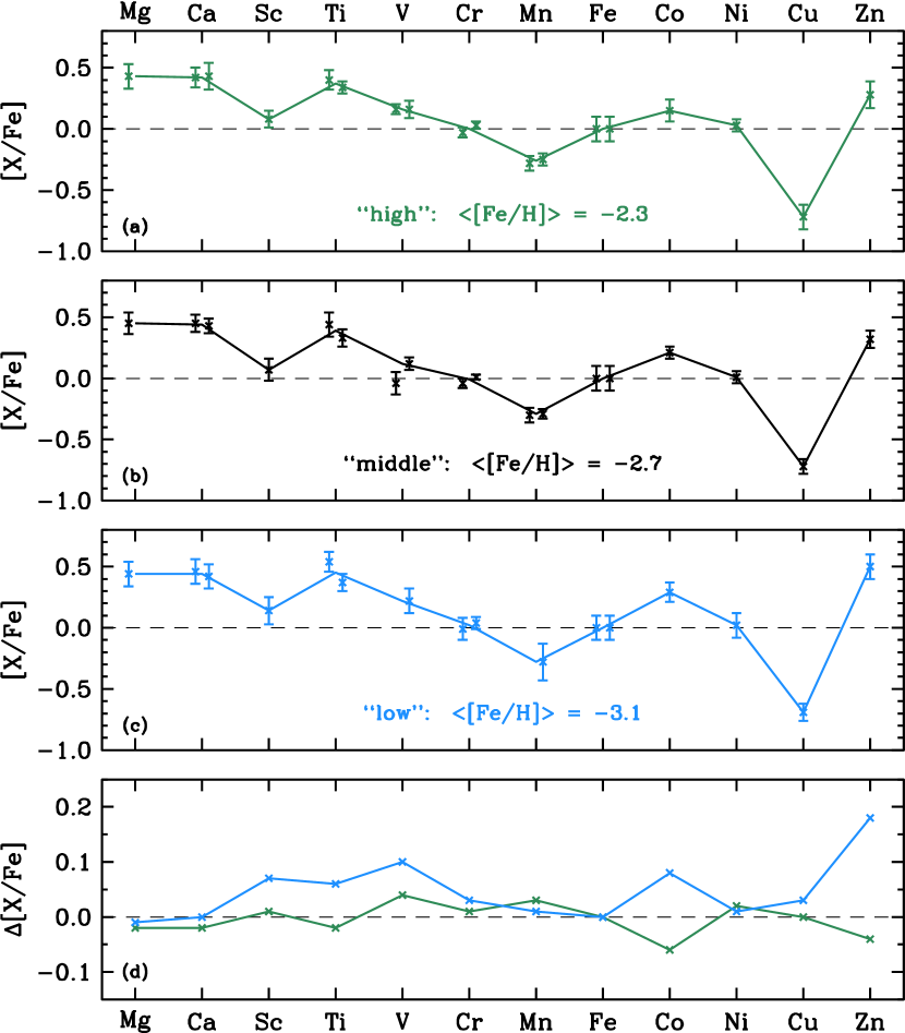
Figure 6: Final species and elemental abundances for the low, middle, and high metallicity groups of our sample. Panels (a), (b), and (c) show species abundance points (Table 3) and elemental abundance lines (Table 4) for the high, middle, and low abundance groups. For elements with abundances from two species, the points for neutral and ionized values are shifted by small amounts leftward and rightward of the element position, respectively. Panel (d) shows differences between the abundances of the high and middle metallicity groups (green line and points) and between those of the low and middle metallicity groups (blue line and points).

Table 4 summarizes our elemental abundance results. Column 2 of the table contains the mean abundances for our entire 37 star sample, drawing from the species abundances of Table 3. For elements represented by only one species (Sc, Co, Ni, Cu, and Zn) the elemental abundances are simply the species values. For Ca, Ti, Cr, and Mn the elemental abundances are averages of the neutral and ionized species abundances. And for V the ion abundance is exclusively used for the element because we had relatively few stars with neutral abundances for this element. Table 4 also lists in columns 3$-$5 the elemental abundance means for the 12 stars with lowest metallicities in our sample, the 12 stars with “middle” metallicities, and the 13 stars with highest metallicities. The mean metallicities for each group are listed in the column headers.

In Figure 6 we illustrate these abundance results. In panels (a)$-$(c) we show the abundances for the 3 metallicity groups, using data from Tables 3 and 4. The dots with error bars are individual species abundances. For those elements with both ionic and neutral measurements the abundance determinations agree well. Inspection of these panels reveals overall abundance pattern agreement among the metallicity groups. In particular, as earlier suggested by Cowan et al. (2020) with a sample of only four stars but including HST/STIS spectra below 3000 Å, a distinct non-solar abundance pattern is evident:

• the traditional $\alpha$ elements Mg and Ca are overabundant with respect to Fe by $\simeq$0.4 dex. This confirms decades of previous work on these elements; our contribution is the extensive use of Ca ii transitions to bolster our abundance for this element.

• the lightest Fe-group elements Sc, Ti, and V are overabundant with respect to Fe. This issue was discussed by Sneden et al. (2016) and Cowan et al. (2020); here we add a large stellar sample to the discussion. We will consider this in more detail below.

• Mn is underabundant, but by less than 0.3 dex. This is much smaller than the results presented in early abundance studies of metal-poor stars. Neglect of the Mn i ground state lines and emphasis on Mn ii abundances, as discussed in §3.3, leads to this mild Mn deficiency conclusion.

• Co appears to be mildly overabundant, especially in the lowest metallicity stars. Caution should accompany interpretation of this result, as Cowan et al. (2020) found no [Co/Fe] anomalies when studying UV Co ii lines in 3 stars with [Fe/H] $\simeq$ $-$3. The apparent overabundances from our optical-range Co i transitions may be evidence of line formation issues rather than real abundance effects.

• Zn is significantly overabundant in all 3 metallicity groups.

In panel (d) of Figure 6 we compare the elemental abundances of the low and high metallicity groups to those of the middle group, to illustrate trends with decreasing [Fe/H]. There is little difference between the middle and high metallicity groups. However, it is clear (see also Table 4) that abundance ratios are different in the lowest metallicity group: several elements are overabundant with respect to iron. In particular, the Sc, Ti and V anomalies increase with decreasing metallicity. [Co/Fe] and [Zn/Fe] also show significant increases at lower metallicities.

4.1 Elemental Abundance Correlations

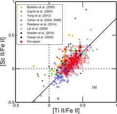
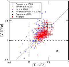
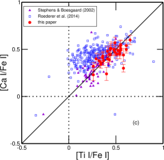
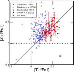
Figure 7: Abundance ratios of 4 elements with respct to [Ti/Fe]. These exhibit likely positive correlations. (a), Sc ii vs. Ti ii; (b), V ii vs. Ti ii; (c), Ca i vs. Ti i; and (d), Zn i vs. Ti i. Sources for the symbols are defined in the figure legends. The horizontal and vertical (dotted) lines denote the solar abundance ratios of each element. The 45^∘ solid line represents perfect correlations between the abundance ratios.

The similarity in the (non-solar) abundance patterns seen in Figure 6 suggests that the abundance ratios of some elements are correlated. Several such correlations are easily seen in Figure 7, pointing to a possible common origin or nucleosynthesis history. As in our past studies (e.g., Sneden et al. 2016; Cowan et al. 2020) we employ Ti as the comparison element. We have included earlier data sets that are identified in the figure legends. These older abundances are only for comparison purposes and are not meant to be a comprehensive listing of all earlier studies. The dotted horizontal and vertical lines indicate solar system values.

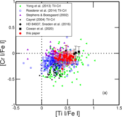
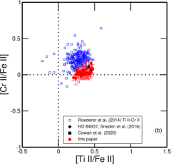
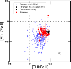
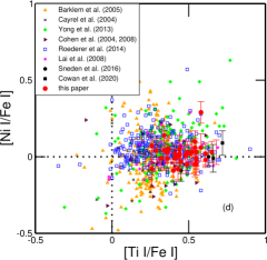
Figure 8: Abundance comparisons indicating no correlations. (a) Cr i vs. Ti i; (b) Cr ii vs. Ti ii; (c) Mn ii vs. Ti ii; (d) Ni i vs. Ti i. Symbols are defined in the panel legends and are consistent with those of Figure 7.

In panel (a) of Figure 7 we have plotted the values of Sc ii and Ti ii as red filled circles with error bars (line-scatter $\sigma$ values). Inspection of these abundances reveals substantial correlation between the two elements. Other data sets generally support the trends in our data, although we have not attempted to apply normalization corrections to align the other results and ours. To emphasize these correlations we have added a line at a 45^∘ angle passing through the midpoint of our data. In panels (b), (c), and (d) we have repeated these steps, although the other elements have been studied in fewer previous papers.

We computed Pearson correlation coefficients for our data. Defining $r$(X,Y) $\equiv$ $r$([X/Fe],[Y/Fe]), we found $r$(Sc ii,Ti ii) = 0.70, $r$(V ii,Ti ii) = 0.61, $r$(Ca i,Ti i) = 0.66, and $r$(Zn i,Ti i) = 0.59, all positive moderate-to-high correlations ($|r|$ $>$ 0.5). By way of contrast the pure $\alpha$ element Mg shows no apparent abundance correlation with Ti: $r$(Mg i,Ti i) = 0.14. The links between Ca, Sc, Ti, V, and Zn appear to be well established. Note particularly that our new data, as well as that from Roederer et al. (2014), suggest a correlation with increasing Ca tracking increasing Ti. This link has not been noted previously. Our confidence in this correlation is increased by the determination of abundances from Ca ii transitions in 25 stars in our sample of 37. The neutral and ion abundances correlate well: $r$([Ca i/Fe],Ca ii/Fe]) = 0.88. Calcium is normally thought to be formed in explosive oxygen or (incomplete) silicon burning (Curtis et al. 2019); based upon this analysis, it may be formed in concert with Ti in early nucleosynthetic environments, preceding most halo star formation. Additional observational abundance data would help to confirm this correlation.

The correlations among [Sc/Fe], [V/Fe], and [Ti/Fe] have been noted previously (e.g., Sneden et al. 2016, Ou et al. 2020, Cowan et al. 2020), but the evidence is even clearer now with the addition of new precise abundance values in a larger sample of metal-poor stars. Ti and V are formed as a result of complete or incomplete Si burning, respectively (Curtis et al. 2019, Ebinger et al. 2020). Although Ti synthesis is complicated and results from several processes in explosive environments (e.g., supernovae, SNe), our results suggest that at early Galactic times the synthesis sites for Fe-peak element production made an overabundance of Ti (on average by 0.3-0.5 dex). While typical core-collapse SNe models have difficulty producing enhanced Ti at early Galactic times (see further comments in §4.3) higher explosion energies in hypernovae can produce larger amounts of certain Fe-peak elements (Umeda & Nomoto, 2002; Kobayashi et al., 2006). This might suggest more energetic hypernovae early in the Galaxy (see Kobayashi et al. 2020, and discussion in Sneden et al. 2016, Cowan et al. 2020).

We find a positive correlation of Zn with Ti, illustrated in panel (d) of Figure 7. Li et al. (2022a) have identified moderate correlations in some of their data between Sc and the alpha elements, as well as between Ti and Zn. We strengthen these conclusions and extend them to additional elements. We caution that there is more scatter in our Zn data than in other elemental abundances and the comparison to the Zn abundances of Roederer et al. (2014) is not encouraging, but there appears to be a possible trend with higher [Zn/Fe] in stars being associated with higher [Ti/Fe] values. Lack of sufficient internally consistent high SNR spectra has previously prevented seeing such a possible correlation, and again, more data will be required to confirm such a correlation.

We examined several other elemental abundance ratios to search for possible correlations that may fortify or negate the positive linkages among the elements discussed above. Four examples are displayed in Figure 8. The computed correlation coefficients are $r$(Cr i,Ti i) = 0.23 (panel a); $r$(Cr ii,Ti ii) = 0.49 (panel b); $r$(Mn ii,Ti ii) = 0.02 (panel c); $r$(Ni i,Ti i) = 0.11 (panel d). These suggest very low positive correlations between Cr and Ti abundances, and no apparent connections between Mn, Ni, and Ti abundances (low correlations are here considered to be $|r|$ $<$ 0.3). These results suggest that the elements Cr, Mn and Ni are not formed in the same manner or nucleosynthesis site as that of Ti. We also note that in panel (a) the derived [Cr i/Fe i] abundance ratios, computed without employing the Cr i resonance lines, is significantly higher than found in previous studies $-$ the new ratios are consistent with solar values; see the discussion in §3.3. It is also apparent from panels (a) and (b) that the new [Cr i/Fe i] values (without resonance lines) are consistent with the [Cr ii/Fe ii] abundance ratios. Inspection of Tables 3 and 4 and discussion in §3.3 also indicate a similar result for neutral and ionized Mn transitions.

4.2 Galactic Abundance Trends

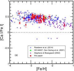
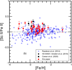
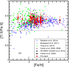
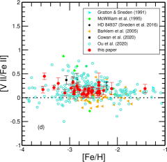
Figure 9: Abundance ratios of various elements versus [Fe/H] metallicity. The symbols are defined in the figure legend and are consistent with the symbols in Figures 7 and 8. The horizontal (dotted) line denotes the solar abundance ratios of each element.

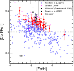
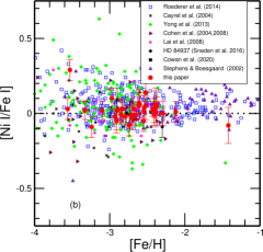
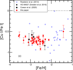
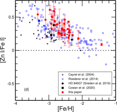
Figure 10: (a): Abundance ratios of various elements versus [Fe/H]. See the figure legend for the data sources. The error bars here are simply the line-scatter $\sigma$ values for each star. The horizontal (dotted) lines in each panel denote the solar abundance ratio.

In Figures 9 and 10 we illustrate abundance trends as functions of metallicity for the elements in our new survey. Here we comment on them individually.

Calcium: Our [Ca/Fe] trend (Figure 9 panel a) is consistent with earlier results from Stephens & Boesgaard (2002), Roederer et al. (2014), and Den Hartog et al. (2021), all plotted in this panel. These data show values above solar for a wide metallicity range. The downward trend in [Ca/Fe] at higher metallicity has long been interpreted as due to increased production of iron from Type Ia SNe. Below metallicity [Fe/H] $\sim$ $-$2 the Ca overabundance qualitatively appears to plateau at [Ca/Fe] $\sim$ 0.5 if all data sets in Figure 9 are included. There may be a slight increase in Ca overabundance with decreasing metallicity in our stellar sample, but it is not statistically meaningful: $r$(Ca i,[Fe/H]) = 0.21, consistent with essentially no trend with metallicity. Future studies of [Ca/Fe] at the lowest metallicities are required to pursue this point.

Scandium: Panel (b) of Figure 9 shows relatively large star-to-star scatter in our [Sc ii/Fe ii] ratios at a given [Fe/H] metallicity, and generally higher abundance ratios than those reported by Roederer et al. (2014) at the lowest metallicities. Our data suggest no significant metallicity trend for Sc.

Titanium: There is little indication of Ti overabundance variations with metallicity in our sample, as illustrated in Figure 9 panel (c), and as computed in a correlation coefficient: $r$(Ti ii,[Fe/H]) = 0.12. The [Ti/H] vs [Fe/H] correlation in Figure 15 of B11 show a tight correlation between Ti and Fe abundances over almost 4 orders of magnitude in [Fe/H] in their 117 stars. They found a slope of 0.86 $\pm$ 0.01. Results from other studies shown in Figure 9 panel (c) appear to be divergent at lowest metallicities; this should be pursued in future studies. At metallicities [Fe/H] $\lesssim$ $-$2.5 the star-to-star scatters increase within individual surveys. The disagreements in scale among the surveys do not inspire confidence in the published [Ti/Fe] abundance ratios at lowest metallicities. Resolution of this issue is beyond the scope of our study.

Vanadium: The [V ii/Fe] relative abundances shown in panel (d) of Figure 9 have little change with metallicity. $r$(V ii,[Fe/H]) = $-$0.30, at the low edge of a possible trend with decreasing [Fe/H].

Cobalt: In panel (a) of Figure 10 we correlate [Co i/Fe i] with metallicity. The trend of rising Co abundance ratios at low [Fe/H] is easy to see and strongly backed statistically: $r$(Co i,[Fe/H]) = $-$0.84. The apparent Co overabundances in the most metal-deficient stars was not an artifact of weak Co i line measurement errors. $EW$s for many Co i transitions were easily measured even in our lowest metallicity stars. Most lines detectable in these stars have wavelengths in the 3400$-$3600 Å spectral domain. But the original B11 requirement to have reasonable SNR down to 3100 Å ensured very good SNR values in this part of the near-UV range. Measurement of Co i lines with log $RW$ $\gtrsim$ $-$5.8 was not difficult.

The increasing [Co/Fe] trend with decreasing metallicity, shared by other surveys included in panel (a) of Figure 10, has been known since the survey of very metal-poor giants by McWilliam et al. (1995); see their Figure 11. However, as noted in §3.3 and discussed in detail by Cowan et al. (2020), this increase in [Co i/Fe] is not shared by [Co ii/Fe] values. Unfortunately, the ion abundances are only available via HST/STIS spectra, inaccessible in this study and not likely to be increased in the foreseeable future. An NLTE investigation by Bergemann et al. (2010) suggested that LTE [Co i/Fe] values should be $increased$ by as much as +0.4 dex very low metallicities, which would significantly increase the neutral/ion Co abundance clash. We regard the Co abundance problem as unsolved at this point, and urge additional NLTE investigations.

Nickel: Inspection of panel (b) of Figure 10 immediately suggests no evolution of [Ni i/Fe] values over the entire $-$4 $<$ [Fe/H] $<$ $-$1 metallicity range in any of the many studies of this element. Our correlation coefficient confirms the qualitative assessment: $r$(Ni i,[Fe/H]) = $-$0.01, excluding the one very discordant high value for G 275-4 ([Fe/H] = $-$3.53). The Ni abundance is well-determined in G 275-4, but it appears to be out of the mainstream of values for this element at low metallicity. However only two stars of our sample have [Fe/H] $\lesssim$ $-$3.3; general conclusions on the Ni abundance in G 275-4 await a larger-sample study of similar stars.

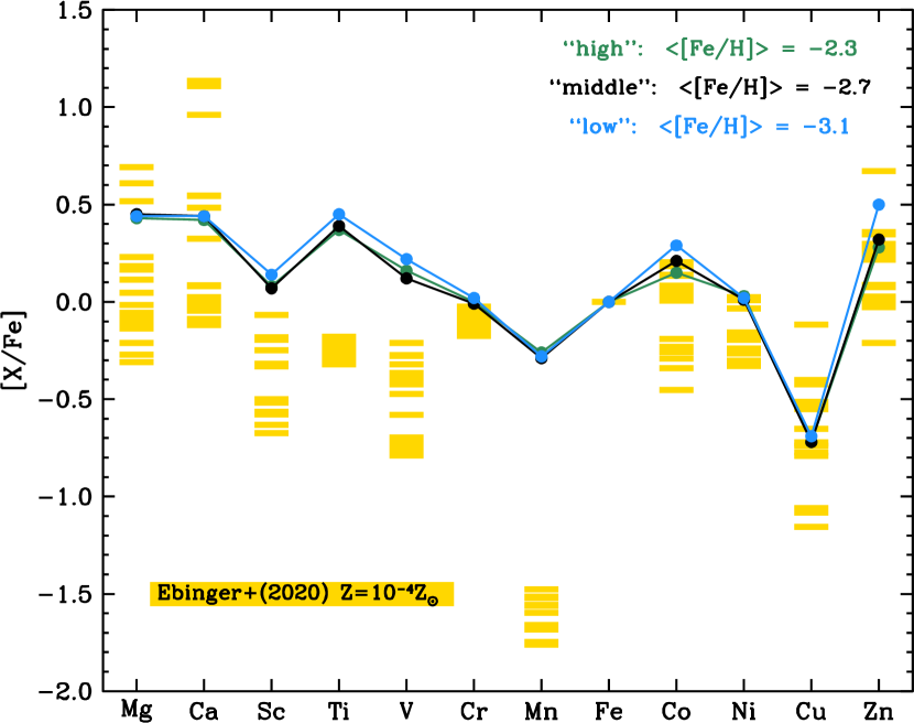
Figure 11: Supernovae nucleosynthesis predictions from Ebinger et al. (2020) for low-metallicity stars compared to average abundance determinations of the stars from this paper (Table 4).

Copper: Our [Cu i/Fe] values are based on LTE analyses, and as discussed in §3.3 they are likely to be deficient by $\sim$0.5 dex compared to values derived in NLTE. Thus our mean value, $\langle$[Cu i/Fe]$\rangle$ = $-$0.71 ($\sigma$ = 0.08), might turn out to be $\sim-$0.2. Our Cu abundances appear to be relatively constant. Note the lack of many literature sources on Cu in very low-metallicity stars. There are few Cu i lines in optical wavelength regions redward of 4000 Å. The strongest line at 5105.5 Å is too weak to be reliably detected in any of our stars with [Fe/H] $<$ $-$2. Our Cu abundances are derived from the resonance lines at $\lambda$3247,3273. Most abundance surveys of metal-poor stars do not extend blueward to these wavelengths.

Zinc: Abundance evolution of Zn with metallicity is shown in panel (d) of Figure 10. We confirm increasing [Zn i/Fe] abundance with decreasing [Fe/H] first identified in the large-sample survey of metal-poor red giants by Cayrel et al. (2004). The correlation coefficient for our data agrees with the visual impression: $r$(Zn i,[Fe/H]) = $-$0.74 . The lines of Zn i at $\lambda$4722,4810 are often very weak in our spectra, but our analyses by both EW and synthetic spectra agree well. Seeing the same trend in both main sequence and red giant stars strengthens the conclusion that this is a genuine abundance result, not an analytical artifact. While there is star-to-star scatter in our data and in literature results, it is clear that relative [Zn/Fe] production increases with decreasing metallicity.

4.3 Nucleosynthesis Origins

We have shown from a large sample of 37 very metal-poor main sequence turnoff stars that high correlations exist between the elements Ca, Sc, Ti, V and Zn, suggesting they were formed in concert near the beginning of our Galaxy. These elements are synthesized in several processes; see Curtis et al. (2019) and discussion in Sneden et al. (2016), Cowan et al. (2020). However, the observed correlations might suggest that one specific process (perhaps complete or incomplete silicon burning) might be the dominant nucleosynthesis path for these particular elements in early Galactic SNe.

We compare our measured abundance values with recent SNe calculations from Ebinger et al. (2020) in Figure 11. They show nucleosynthesis yields from core-collapse SNe for solar and low-metallicity ([Fe/H] = $-$4) cases; the latter values might be typical for the progenitors to the stars of our survey. We have illustrated a range of their model predictions (indicated by vertical, often overlapping horizontal bars) for each element from Mg-Zn. It is seen that they correctly predict values for the low-metallicity stars for many of our observed elements, particularly the heavier ones (Z $\geq$ 26). It is noteworthy that they are able to reproduce our observed rises in [Co/Fe] and [Zn/Fe] for all stars in the sample. The exceptions are Sc, Ti, V, and Mn, where the observed abundances [X/Fe] are larger than model predictions. These overabundances, particularly for Ti, have been well-known for some time. It is interesting that these divergences between calculations and observations occur for elements below iron (Z $<$ 26). This, in turn, might suggest some differences (i.e., decreases) in iron production (with respect to elements such as Ti) at these very low metallicities, and perhaps for the earliest Galactic SNe (while iron production in the Galaxy today is primarily from Type Ia SNe, core-collapse SNe were responsible for the earliest Galactic iron synthesis.) We also note new model predictions for Mg and Ca from Ebinger et al. (2020) also replicate our abundance determinations for those elements in the sample stars. In the future it will be important to determine if there are rises in the abundances of those two elements at the lowest metallicities. Our new results $-$ at an elemental abundance accuracy of 0.1 dex $-$ could provide constraints, not only at low metallicities but also at high metallicities, for SNe models early in Galactic history.

4.4 Trends with Kinematics

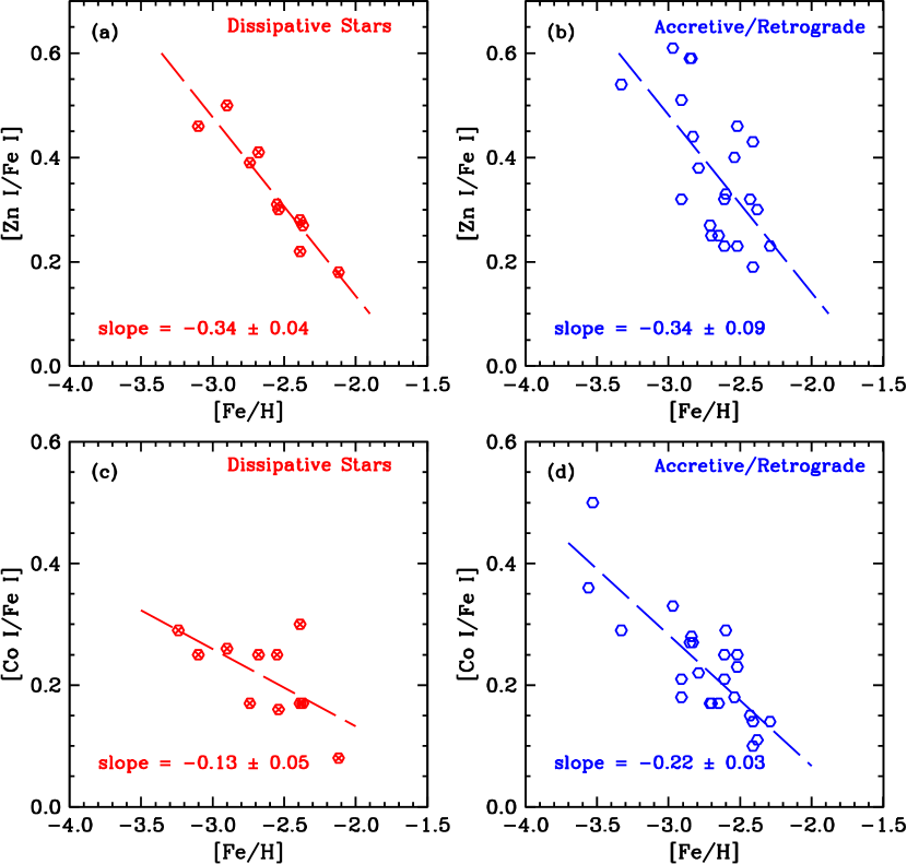
Figure 12: Abundance ratios of Zn and Co with respect to [Fe/H] metallicity for 2 kinematic groups. Panel (a) shows the [Zn i/Fe i] values for the dissipative stars and panel (b) shows them for the accretive retrograde stars. Panels (c) and (d) repeat these plots for [Co i/Fe i]. The dashed lines in each panel represent linear regression lines through the data.

[Zn/Fe] is overabundant in all three metallicity groups displayed in Figure 6. This is also true to a lesser extent for [Co/Fe]. We decided to examine the effects of stellar populations or Galactic components/origins on these trends. In B11 their 117 stars were divided into groups based on their kinematic properties. One stellar group was connected to the dissipative collapse of the Galaxy discussed by Eggen et al. (1962) includes stars from the classical thick disk and halo. Other stars are associated with a population that was accreted as proposed first by Searle & Zinn (1978) which are mainly halo stars. Some of those stars are on retrograde orbits. The details of the classifications can be found in B11. Our sample of 37 stars here has 11 in the dissipative category and 25 that are classified in the accretive population, of which 13 are also on retrograde orbits. In Table 5 we list the stars and their Zn and Co abundance ratios in the two kinematic groups. One program star not included in this table is BD $-$13 3442; it lacked orbital/velocity information to be classified kinematically by B11.

In Figure 12 we show correlations of [Zn i/Fe i] with [Fe/H] for the dissipative component (panel a) and accretive component (panel b). The mean trends with [Fe/H] are nearly identical. But the star-to-star scatter is extremely small over an order of magnitude in metallicity for stars of the dissipative population. Inspection of panel (b) reveals a significantly larger scatter in stars that were accreted into the Milky Way. These representatives of nearby dwarf spheroidal galaxies have less uniform origins and come from different chemical environments. This supposition is reinforced by the larger scatter in their [Zn i/Fe i] ratios.

The situation for Co is shown in Figure 12 panels (c) and (d). A steeper slope with Fe for the accretive group is apparent, as well as a somewhat larger spread in [Co i/Fe i]. This could be attributed to the more diverse origin of this aggregate of stars. However, we repeat here our concerns on the apparent clash between neutral and ionized Co species in our previous study (Cowan et al., 2020). It is not clear how much to trust the [Co i/Fe i] results presented here.

Our understanding of the chemical and dynamical complexity of the Milky Way stellar halo has been revolutionized in recent years by the availability of large chemical abundance surveys and precise astrometric data (e.g., Naidu et al. 2020, Li et al. 2022b, Limberg et al. 2021, Myeong et al. 2022, Horta et al. 2023). Our two-group categorization of stellar kinematics is appropriate here for simplicity and for our small sample size, but a deeper analysis with larger data sets for Co and Zn will be welcome. The results of this section suggest that there may be different abundance behavior among stars with different kinematics. Future studies along these lines may provide additional insight into the nature of the supernova progenitors that enriched the stars in our sample.

5 SUMMARY

We have determined precise elemental abundance values for Mg, Ca, and Fe-group (Z = 21$-$30) elements for 37 warm, high gravity very metal-poor stars ($-$3.4 $\leq$ [Fe/H] $\leq$ $-$2.1). We have used high S/N and high spectral resolution echelle spectra which extend into the near-UV at 3050 Å. We have measured 350+ spectral lines in each star of our sample. Our analysis makes use of high quality lab data and includes hyperfine structure where needed. The abundances were found in LTE computations with various techniques for neutral and/or ionized states for 12 elements. For most elements there is little spread with small star-to-star scatter. The agreement in abundance from neutral and ionized species is very good for Ca, Ti, V, Cr, Mn, and Fe.

We have divided the stars into 3 metallicity groups and present the mean abundances for each set. For each group the trends in [X/Fe] are similar. The light Fe-peak elements, Sc, Ti, and V, are overabundant relative to Fe compared to solar ratios. Our study confirms and extends the apparent linkage between these overabundances previously found in other much smaller samples. While Mn is underabundant, Co and especially Zn are overabundant. We have examined abundance correlations and find an indication of a new correlation between Zn and Ti. This overabundance connection now includes Zn in the most metal-poor stars in our sample. There are also indications that both Ca and Zn may form in concert with Ti.

More observational determinations, as well as theoretical studies outside the scope of this paper will be needed to understand the production mechanism and history for these elements. Perhaps even more important will be NLTE abundance studies covering wide ranges in model atmosphere parameters for large numbers of atomic transitions. Our abundances derived from Cr i, Mn i, Cu i, and probably Co i point to clear limits to the reliability of LTE analyses of Fe-group elements in metal-poor stars.

Employing the abundances data of our survey, we have examined the Galactic chemical evolution of a number of elements. While most [X/Fe] ratios either are constant with [Fe/H] metallicity or change very modestly, increases in especially [Zn/Fe] are apparent in the lowest metallicity stars. These new results could provide important constraints on nucleosynthesis and SNe models early in Galactic history.

Table 1: Model Atmosphere Parameters

Star	Teff	log g	$\xi_{\rm t}$	[Fe/H]	$\sigma$	#lines	[Fe/H]	$\sigma$	#lines
	K		km s-1	Fe i	Fe i	Fe i	Fe ii	Fe ii	Fe ii
G 64-12	6100	3.90	1.30	-3.60	0.11	113	-3.51	0.13	12
G 275-4	6050	4.20	1.10	-3.57	0.09	85	-3.49	0.11	7
G 64-37	6250	4.00	1.20	-3.34	0.09	98	-3.31	0.09	12
LP 831-70	6005	4.10	1.20	-3.28	0.09	121	-3.20	0.10	11
G 206-34	6000	4.00	1.20	-3.14	0.08	144	-3.05	0.11	15
BD +9 2190	6225	3.70	1.40	-3.01	0.10	118	-2.92	0.09	18
BD $-$13 3442	6250	3.60	1.50	-2.94	0.09	115	-2.92	0.10	17
BD +20 2030	6000	3.50	1.50	-2.95	0.10	138	-2.87	0.12	17
LP 815-43	6350	4.00	1.30	-2.97	0.10	117	-2.85	0.12	16
BD +3 740	6200	3.60	1.50	-2.95	0.11	137	-2.85	0.09	19
BD +1 2341	6350	4.00	1.40	-2.89	0.10	116	-2.81	0.10	17
LP 651-4	6275	4.00	1.30	-2.86	0.10	111	-2.82	0.08	12
BD +26 2621	6275	4.10	1.40	-2.87	0.09	139	-2.79	0.09	19
LP 553-62	6200	3.70	1.40	-2.83	0.10	132	-2.74	0.11	17
G 92-6	6275	3.90	1.40	-2.76	0.10	144	-2.71	0.10	18
G 26-12	5950	3.75	1.25	-2.73	0.09	144	-2.69	0.10	17
LP 635-14	6150	3.55	1.40	-2.72	0.10	148	-2.67	0.11	21
G 4-37	6200	4.00	1.30	-2.71	0.11	153	-2.64	0.10	17
G 181-28	5950	4.00	1.25	-2.68	0.10	163	-2.62	0.11	16
G 88-10	6100	4.00	1.25	-2.64	0.09	155	-2.58	0.12	19
G 108-58	5800	4.30	1.20	-2.63	0.11	146	-2.59	0.09	16
BD +24 1676	6300	3.70	1.50	-2.62	0.10	162	-2.58	0.09	21
BD $-$4 3208	6200	3.65	1.45	-2.59	0.10	154	-2.51	0.09	20
BD +13 3683	5500	3.10	1.25	-2.54	0.11	147	-2.54	0.08	16
G 126-52	6200	3.80	1.30	-2.58	0.10	159	-2.49	0.09	20
G 201-5	6150	3.90	1.20	-2.53	0.10	162	-2.51	0.10	21
G 59-24	6100	4.30	1.30	-2.55	0.10	146	-2.49	0.12	15
BD +2 3375	6025	3.90	1.25	-2.43	0.10	157	-2.43	0.09	17
LTT 1566	6125	3.90	1.20	-2.42	0.11	169	-2.40	0.08	19
G 75-56	6100	3.70	1.25	-2.44	0.09	160	-2.38	0.08	18
BD $-$10 388	6350	4.00	1.50	-2.43	0.11	171	-2.35	0.08	20
BD $-$14 5850	5775	4.10	1.25	-2.35	0.12	288	-2.42	0.16	25
LP 752-17	5950	3.20	1.50	-2.39	0.09	150	-2.37	0.09	19
BD +36 2964	6150	3.70	1.35	-2.39	0.09	156	-2.34	0.08	19
G 130-65	6100	3.90	1.35	-2.29	0.10	154	-2.28	0.09	19
G 20-24	6200	3.60	1.30	-2.14	0.10	188	-2.10	0.10	25
BD +51 1696	5695	4.50	1.00	-1.40	0.12	134	-1.44	0.08	17

Table 2: Abundances for Individual Stars

Star	[Fe/H]	Species	[X/Fe]	$\sigma$	#lines
G64-12	$-$3.56	Mg i	0.57	0.10	7
G64-12	$-$3.56	Ca i	0.60	0.05	13
G64-12	$-$3.56	Ca ii	0.54	0.04	5
G64-12	$-$3.56	Sc ii	0.11	0.04	11
G64-12	$-$3.56	Ti i	0.65	0.07	6
G64-12	$-$3.56	Ti ii	0.40	0.12	62
G64-12	$-$3.56	V i	$\cdots$	$\cdots$	$\cdots$
G64-12	$-$3.56	V ii	0.17	0.07	6
G64-12	$-$3.56	Cr i	0.17	0.07	6
G64-12	$-$3.56	Cr i no 0eV	$-$0.13	0.08	6
G64-12	$-$3.56	Cr ii	$-$0.06	0.09	2

Note. — This table is available in its entirety in machine-readable form.

Table 3: Mean Species Abundance Ratios

Element	$\langle$[X/Fe]$\rangle$	$\sigma$	#stars	$\langle$[X/Fe]$\rangle$	$\sigma$	#stars
	I	I	I	II	II	II
Mg	0.44	0.09	37	$\cdots$	$\cdots$	$\cdots$
Ca	0.44	0.09	37	0.42	0.11	25
Sc	$\cdots$	$\cdots$	$\cdots$	0.10	0.09	37
Ti	0.46	0.10	37	0.35	0.06	37
V	0.13	0.09	7	0.17	0.08	37
Cr	$-$0.03	0.06	37	0.03	0.04	37
Mn	$-$0.28	0.06	19	$-$0.27	0.09	37
Co	0.21	0.02	37	$\cdots$	$\cdots$	$\cdots$
Ni	0.02	0.07	37	$\cdots$	$\cdots$	$\cdots$
Cu	$-$0.71	0.08	36	$\cdots$	$\cdots$	$\cdots$
Zn	0.35	0.13	34	$\cdots$	$\cdots$	$\cdots$

Table 4: Mean Element Abundance Ratios in Three Metallicity Bins

Element	$\langle$[X/Fe]$\rangle$	$\langle$[X/Fe]$\rangle$	$\langle$[X/Fe]$\rangle$	$\langle$[X/Fe]$\rangle$
$\langle$[Fe/H]$\rangle$	all	$-$3.09	$-$2.67	$-$2.32
Mg	0.44	0.44	0.45	0.43
Ca	0.43	0.44	0.44	0.42
Sc	0.10	0.14	0.07	0.08
Ti	0.40	0.45	0.39	0.37
V	0.17	0.22	0.12	0.16
Cr	0.00	0.02	$-$0.01	0.00
Mn	$-$0.27	$-$0.28	$-$0.29	$-$0.26
Fe	0.00	0.00	0.00	0.00
Co	0.21	0.29	0.21	0.15
Ni	0.02	0.02	0.01	0.03
Cu	$-$0.71	$-$0.69	$-$0.72	$-$0.72
Zn	0.35	0.50	0.32	0.28

Table 5: Co and Zn in Kinematic Groups

Star	[Fe/H]	[Co i/Fe i]	[Zn i/Fe i]
Dissipative Group
LP 831-70	$-$3.24	0.29	$\cdots$
G 206-34	$-$3.10	0.25	0.46
BD+3-740	$-$2.90	0.26	0.50
G 92-6	$-$2.74	0.17	0.39
G 4-37	$-$2.68	0.25	0.41
BD $-$4-3208	$-$2.55	0.25	0.31
BD +13 3683	$-$2.54	0.16	0.30
BD $-$10-388	$-$2.39	0.30	0.28
BD $-$14-5850	$-$2.39	0.17	0.22
BD +36-2964	$-$2.37	0.17	0.27
G 20-24	$-$2.12	0.08	0.18
Accretive Group
G 64-12	$-$3.56	0.36	$\cdots$
G 275-4	$-$3.53	0.50	$\cdots$
G 64-37	$-$3.33	0.29	0.54
BD +9-2190	$-$2.97	0.33	0.61
BD +20-2030	$-$2.91	0.18	0.51
LP 815-43	$-$2.91	0.21	0.32
BD +11-2341	$-$2.85	0.27	0.59
LP 651-4	$-$2.84	0.28	0.59
BD +26-2621	$-$2.83	0.27	0.44
LP 553-62	$-$2.79	0.22	0.38
G 26-12	$-$2.71	0.17	0.27
LP 635-14	$-$2.70	0.17	0.25
G 181-21	$-$2.65	0.17	0.25
G 88-10	$-$2.61	0.25	0.32
G 108-58	$-$2.61	0.21	0.23
BD +24-1676	$-$2.60	0.29	0.33
G 126-52	$-$2.54	0.18	0.40
G 201-5	$-$2.52	0.23	0.23
G 59-24	$-$2.52	0.25	0.46
BD +2-3375	$-$2.43	0.15	0.32
LTT 1566	$-$2.41	0.10	0.19
G 75-56	$-$2.41	0.14	0.43
LP 752-17	$-$2.38	0.11	0.30
G 130-65	$-$2.29	0.14	0.23

References

- Andrievsky et al. (2018) Andrievsky, S., Wallerstein, G., Korotin, S., et al. 2018, PASP, 130, 024201
- Asplund et al. (2009) Asplund, M., Grevesse, N., Sauval, A. J., & Scott, P. 2009, ARA&A, 47, 481
- Barklem et al. (2005) Barklem, P. S., Christlieb, N., Beers, T. C., et al. 2005, A&A, 439, 129
- Belmonte et al. (2017) Belmonte, M. T., Pickering, J. C., Ruffoni, M. P., et al. 2017, ApJ, 848, 125
- Bensby & Lind (2018) Bensby, T., & Lind, K. 2018, A&A, 615, A151
- Bergemann & Cescutti (2010) Bergemann, M., & Cescutti, G. 2010, A&A, 522, A9
- Bergemann & Gehren (2008) Bergemann, M., & Gehren, T. 2008, A&A, 492, 823
- Bergemann et al. (2010) Bergemann, M., Pickering, J. C., & Gehren, T. 2010, MNRAS, 401, 1334
- Boesgaard et al. (2011) Boesgaard, A. M., Rich, J., Levesque, E. M., & Bowler, B. P. 2011, ApJ, 743, 140
- Cayrel et al. (2004) Cayrel, R., Depagne, E., Spite, M., et al. 2004, A&A, 416, 1117
- Cohen et al. (2008) Cohen, J. G., Christlieb, N., McWilliam, A., et al. 2008, ApJ, 672, 320
- Cohen et al. (2004) —. 2004, ApJ, 612, 1107
- Cowan et al. (2021) Cowan, J. J., Sneden, C., Lawler, J. E., et al. 2021, Reviews of Modern Physics, 93, 015002
- Cowan et al. (2020) Cowan, J. J., Sneden, C., Roederer, I. U., et al. 2020, ApJ, 890, 119
- Curtis et al. (2019) Curtis, S., Ebinger, K., Frohlich, C., et al. 2019, ApJ, 870, 2
- Den Hartog et al. (2019) Den Hartog, E. A., Lawler, J. E., Sneden, C., Cowan, J. J., & Brukhovesky, A. 2019, ApJS, 243, 33
- Den Hartog et al. (2021) Den Hartog, E. A., Lawler, J. E., Sneden, C., et al. 2021, ApJS, 255, 27
- Den Hartog et al. (2011) Den Hartog, E. A., Lawler, J. E., Sobeck, J. S., Sneden, C., & Cowan, J. J. 2011, ApJS, 194, 35
- Den Hartog et al. (2014) Den Hartog, E. A., Ruffoni, M. P., Lawler, J. E., et al. 2014, ApJS, 215, 23
- Ebinger et al. (2020) Ebinger, K., Curtis, S., Ghosh, S., et al. 2020, ApJ, 888, 91
- Eggen et al. (1962) Eggen, O. J., Lynden-Bell, D., & Sandage, A. R. 1962, ApJ, 136, 748
- Fitzpatrick & Sneden (1987) Fitzpatrick, M. J., & Sneden, C. 1987, in Bulletin of the American Astronomical Society, Vol. 19, Bulletin of the American Astronomical Society, 1129
- Gaia Collaboration et al. (2016) Gaia Collaboration, Prusti, T., de Bruijne, J. H. J., et al. 2016, A&A, 595, A1
- Gaia Collaboration et al. (2022) Gaia Collaboration, Vallenari, A., Brown, A. G. A., et al. 2022, arXiv e-prints, arXiv:2208.00211
- Gratton & Sneden (1991) Gratton, R. G., & Sneden, C. 1991, A&A, 241, 501
- Holmbeck et al. (2018) Holmbeck, E. M., Beers, T. C., Roederer, I. U., et al. 2018, ApJL, 859, L24
- Horta et al. (2023) Horta, D., Schiavon, R. P., Mackereth, J. T., et al. 2023, MNRAS, 520, 5671
- Kobayashi et al. (2020) Kobayashi, C., Karakas, A. I., & Lugaro, M. 2020, ApJ, 900, 179
- Kobayashi et al. (2011) Kobayashi, C., Karakas, A. I., & Umeda, H. 2011, MNRAS, 414, 3231
- Kobayashi et al. (2006) Kobayashi, C., Umeda, H., Nomoto, K., Tominaga, N., & Ohkubo, T. 2006, ApJ, 653, 1145
- Korotin (2018) Korotin, S. 2018, MNRAS, 480, 965
- Kramida et al. (2022) Kramida, A., Yu. Ralchenko, J. Reader, & and NIST ASD Team. 2022, NIST Atomic Spectra Database (version 5.10), [Online]. Available: https://physics.nist.gov/asd [2023, March 7] National Institute of Standards and Technology, Gaithersburg, MD., doi:https://doi.org/10.18434/T4W30F
- Kramida et al. (2019) Kramida, A., Yu. Ralchenko, Reader, J., & and NIST ASD Team. 2019, NIST Atomic Spectra Database (version 5.7.1), [Online]. Available: https://physics.nist.gov/asd [Aug 11 2020] National Institute of Standards and Technology, Gaithersburg, MD.
- Kurucz (2011) Kurucz, R. L. 2011, Canadian Journal of Physics, 89, 417
- Kurucz (2018) Kurucz, R. L. 2018, in Astronomical Society of the Pacific Conference Series, Vol. 515, Workshop on Astrophysical Opacities, ed. C. Mendoza, S. Turck-Chiéze, & J. Colgan, 47
- Lai et al. (2008) Lai, D. K., Bolte, M., Johnson, J. A., et al. 2008, The Astrophysical Journal, 681, 1524
- Lawler et al. (2018) Lawler, J. E., Feigenson, T., Sneden, C., Cowan, J. J., & Nave, G. 2018, ApJS, 238, 7
- Lawler et al. (2013) Lawler, J. E., Guzman, A., Wood, M. P., Sneden, C., & Cowan, J. J. 2013, ApJS, 205, 11
- Lawler et al. (2019) Lawler, J. E., Hala, Sneden, C., et al. 2019, ApJS, 241, 21
- Lawler et al. (2015) Lawler, J. E., Sneden, C., & Cowan, J. J. 2015, ApJS, 220, 13
- Lawler et al. (2009) Lawler, J. E., Sneden, C., Cowan, J. J., Ivans, I. I., & Den Hartog, E. A. 2009, ApJS, 182, 51
- Lawler et al. (2017) Lawler, J. E., Sneden, C., Nave, G., et al. 2017, ApJS, 228, 10
- Lawler et al. (2014) Lawler, J. E., Wood, M. P., Den Hartog, E. A., et al. 2014, ApJS, 215, 20
- Li et al. (2022a) Li, H., Aoki, W., Matsuno, T., et al. 2022a, ApJ, 931, 147
- Li et al. (2022b) Li, T. S., Ji, A. P., Pace, A. B., et al. 2022b, ApJ, 928, 30
- Limberg et al. (2021) Limberg, G., Rossi, S., Beers, T. C., et al. 2021, ApJ, 907, 10
- McWilliam et al. (1995) McWilliam, A., Preston, G. W., Sneden, C., & Searle, L. 1995, AJ, 109, 2757
- Minelli et al. (2021) Minelli, A., Mucciarelli, A., Massari, D., et al. 2021, ApJ, 918, L32
- Moore et al. (1966) Moore, C. E., Minnaert, M. G. J., & Houtgast, J. 1966, The solar spectrum 2935 A to 8770 A (National Bureau of Standards Monograph, Washington: US Government Printing Office (USGPO))
- Myeong et al. (2022) Myeong, G. C., Belokurov, V., Aguado, D. S., et al. 2022, ApJ, 938, 21
- Naidu et al. (2020) Naidu, R. P., Conroy, C., Bonaca, A., et al. 2020, ApJ, 901, 48
- Ou et al. (2020) Ou, X., Roederer, I. U., Sneden, C., et al. 2020, ApJ, 900, 106
- Placco et al. (2021) Placco, V. M., Sneden, C., Roederer, I. U., et al. 2021, linemake: Line list generator, ascl:2104.027
- Reddy & Lambert (2008) Reddy, B. E., & Lambert, D. L. 2008, MNRAS, 391, 95
- Roederer & Barklem (2018) Roederer, I. U., & Barklem, P. S. 2018, ApJ, 857, 2
- Roederer et al. (2014) Roederer, I. U., Preston, G. W., Thompson, I. B., et al. 2014, AJ, 147, 136
- Roederer et al. (2022) Roederer, I. U., Lawler, J. E., Den Hartog, E. A., et al. 2022, ApJS, 260, 27
- Ruffoni et al. (2014) Ruffoni, M. P., Den Hartog, E. A., Lawler, J. E., et al. 2014, MNRAS, 441, 3127
- Safronova & Safronova (2011) Safronova, M. S., & Safronova, U. I. 2011, Phys. Rev. A, 83, 012503
- Searle & Zinn (1978) Searle, L., & Zinn, R. 1978, ApJ, 225, 357
- Shi et al. (2018) Shi, J. R., Yan, H. L., Zhou, Z. M., & Zhao, G. 2018, ApJ, 862, 71
- Sneden (1973) Sneden, C. 1973, ApJ, 184, 839
- Sneden et al. (2016) Sneden, C., Cowan, J. J., Kobayashi, C., et al. 2016, ApJ, 817, 53
- Sneden et al. (2009) Sneden, C., Lawler, J. E., Cowan, J. J., Ivans, I. I., & Den Hartog, E. A. 2009, ApJS, 182, 80
- Sobeck et al. (2007) Sobeck, J. S., Lawler, J. E., & Sneden, C. 2007, ApJ, 667, 1267
- Sobeck et al. (2011) Sobeck, J. S., Kraft, R. P., Sneden, C., et al. 2011, AJ, 141, 175
- Stephens & Boesgaard (2002) Stephens, A., & Boesgaard, A. M. 2002, AJ, 123, 1647
- Tody (1986) Tody, D. 1986, in Society of Photo-Optical Instrumentation Engineers (SPIE) Conference Series, Vol. 627, Instrumentation in astronomy VI, ed. D. L. Crawford, 733
- Tody (1993) Tody, D. 1993, in Astronomical Society of the Pacific Conference Series, Vol. 52, Astronomical Data Analysis Software and Systems II, ed. R. J. Hanisch, R. J. V. Brissenden, & J. Barnes, 173
- Umeda & Nomoto (2002) Umeda, H., & Nomoto, K. 2002, ApJ, 565, 385
- Vogt et al. (1994) Vogt, S. S., Allen, S. L., Bigelow, B. C., et al. 1994, in Society of Photo-Optical Instrumentation Engineers (SPIE) Conference Series, Vol. 2198, Instrumentation in Astronomy VIII, ed. D. L. Crawford & E. R. Craine, 362
- Wallerstein & Helfer (1959) Wallerstein, G., & Helfer, H. L. 1959, ApJ, 129, 720
- Wood et al. (2014a) Wood, M. P., Lawler, J. E., Den Hartog, E. A., Sneden, C., & Cowan, J. J. 2014a, ApJS, 214, 18
- Wood et al. (2013) Wood, M. P., Lawler, J. E., Sneden, C., & Cowan, J. J. 2013, ApJS, 208, 27
- Wood et al. (2014b) —. 2014b, ApJS, 211, 20
- Wood et al. (2018) Wood, M. P., Sneden, C., Lawler, J. E., et al. 2018, ApJS, 234, 25
- Yong et al. (2013) Yong, D., Norris, J. E., Bessell, M. S., et al. 2013, ApJ, 762, 26