Hierarchically Structured Matrix Recovery-Based Channel Estimation for RIS-Aided Communications

Abstract

Reconfigurable intelligent surface (RIS) has emerged as a promising technology for improving capacity and extending coverage of wireless networks. In this work, we consider RIS-aided millimeter wave (mmWave) multiple-input and multiple-output (MIMO) communications, where acquiring accurate channel state information is challenging due to the high dimensionality of channels. To fully exploit the structures of the channels, we formulate the channel estimation as a hierarchically structured matrix recovery problem, and design a low-complexity message passing algorithm to solve it. Simulation results demonstrate the superiority of the proposed algorithm and its performance close to the oracle bound.

I Introduction

As a promising technology in future wireless communications, reconfigurable intelligent surface (RIS) is capable of altering the wireless propagation environment to achieve desired channel responses by dynamically adjusting the massive number of passive reflecting elements. With the aid of RIS, wireless networks can achieve high energy efficiency, improve the system capacity and coverage, and enhance massive connectivity [1, 2, 3, 4, 5, 6, 7, 8].

In order to realize the potential of RIS-aided communications, the acquisition of accurate channel state information (CSI) is crucial, which however is very challenging especially in RIS-aided multiple input multiple output (MIMO) systems due to the high dimensionality of channels. The work in [3] studied the uplink channel estimation protocol for a RIS-aided mmWave system, which assumes a random Bernoulli RIS phase matrix. The work in [4] formulated the downlink block fading channel estimation as a sparse matrix factorization and completion problem, where the low-rank or sparsity of channel matrices is exploited. Exploiting the knowledge of the slow-varying channel components and the channel sparsity, a message-passing based algorithm is proposed in [5] to estimate the cascaded channels. The work in [6] proposed a three-phase pilot-based channel estimation framework for RIS-assisted uplink multiuser communications. A sparsity-structured tensor decomposition-based channel estimation method is proposed in [7]. However, the complexity of aforementioned works grows rapidly with the square or cube of the number of RIS elements or has special requirements on the relevant matrices (e.g., the phase matrix of RIS), hindering their applications.

In this letter, to fully exploit the structure of the channels in RIS-aided mmWave MIMO communications, we formulate the channel estimation as a hierarchically destructed matrix recovery problem. To solve the problem, we develop a Bayesian method, which is efficiently implemented with low complexity leveraging unitary approximate message passing (UAMP) [9, 10] and the fast Fourier transform (FFT). Simulation results show that the proposed channel estimator can achieve significant performance gain and delivers performance close to the oracle bound.

Notations-Boldface lower-case and upper-case letters denote vectors and matrices, respectively. Superscripts ${(\bm{A})}^{H}$, ${(\bm{A})}^{*}$and ${(\bm{A})}^{T}$ represent conjugate transpose, conjugate and transpose of $\bm{A}$, respectively. $[\bm{A}]_{i,j}$ represents the ($i,j$)-th element of $\bm{A}$’s, while $[\bm{A}]_{i,:}$ and $[\bm{A}]_{:,j}$ represent its $i$-th row and $j$-th column, respectively. A Gaussian distribution of $x$ with mean $\hat{x}$ and variance $\nu_{x}$ is denoted by $\mathcal{N}(x;\hat{x},\nu_{x}).$ Notations $\otimes$ and $\odot$ represent the Kronecker and Khatri-Rao products, respectively. The notation $\langle\bm{a}\rangle$ denotes an average operation and $\bm{I}_{n}$ denotes a $n\times n$ identity matrix.

II Channel and System Models

We consider a RIS-aided mmWave MIMO uplink system, where a RIS with $N$ passive reflecting elements is equipped between an $M$-antenna BS and $K$ single-antenna users. We neglect the direct propagation path between the BS and users due to the high attenuation caused by unfavorable propagation environments [1]. The channel matrices of BS-RIS and RIS-users are denoted by $\bm{G}\in\mathbb{C}^{M\times N}$ and $\bm{H}\triangleq[\bm{h}_{1},\ldots,\bm{h}_{K}]\in\mathbb{C}^{N\times K}$, respectively. A narrow band geometric channel model is used to characterize the channels $\bm{G}$ and $\bm{h}_{k}$ [1, 5]. A uniform linear array (ULA) is adopted at the BS, and the RIS is an $N_{1}\times N_{2}$ uniform planar array (UPA) with $N=N_{1}N_{2}$ elements. Specifically, $\bm{G}$ can be expressed as

$$\bm{G}=\sqrt{{\rho}(MN)^{-1}}\sum\nolimits_{p=1}^{P}\zeta_{p}\bm{a}_{\mathrm{B}}(\psi_{p})\bm{a}_{\mathrm{R}}^{H}(\vartheta_{p},\gamma_{p}),$$ (1)

where $\rho$ denotes the average path loss, $P$ is the number of paths, $\zeta_{p}$ represents the complex gain associated with the $p$-th path, $\psi_{p}$ denotes the corresponding azimuth angle-of-arrival (AoA), and $\vartheta_{p}$ and $\gamma_{p}$ respectively denote the associated azimuth and elevation angle-of-departure (AoD). The two vectors $\bm{a}_{\mathrm{B}}(\phi_{p})$ and $\bm{a}_{\mathrm{R}}(\vartheta_{p},\gamma_{p})$ are the array response vector of the BS and RIS, respectively, which are given by

$$\bm{a}_{\mathrm{B}}(\psi_{p}) =\bm{e}_{M}(\sin(\psi_{p})),$$ (2)

$$\bm{a}_{\mathrm{R}}(\vartheta_{p},\gamma_{p}) =\bm{e}_{N_{1}}(\cos(\gamma_{p}))\otimes\bm{e}_{N_{2}}(\sin(\gamma_{p})\cos(\vartheta_{p})),$$ (3)

where $\bm{e}_{M}(x)\triangleq{M^{-\frac{1}{2}}}[1,e^{-j\frac{2\pi d}{\lambda}x},\cdots,e^{-j\frac{2\pi d}{\lambda}(M-1)x}]^{T}$, $\lambda$ and $d$ respectively denote the wavelength and antenna spacing with $\lambda=2d$. The RIS-BS channel has a sparse representation in the angular domain, i.e.,

$$\bm{G}=\bm{F}_{1}\bm{\Omega}(\bm{F}_{x}\otimes\bm{F}_{y})^{H}\triangleq\bm{F}_{1}\bm{\Omega}\bm{F}_{2}^{H},$$ (4)

where $\bm{F}_{1}\in\mathbb{C}^{M\times M}$, $\bm{F}_{x}\in\mathbb{C}^{N_{1}\times N_{1}}$ and $\bm{F}_{y}\in\mathbb{C}^{N_{2}\times N_{2}}$ (and $\bm{F}_{2}\in\mathbb{C}^{N\times N}$) are unitary Discrete Fourier Transform (DFT) matrices, $\bm{\Omega}\triangleq[\bm{\omega}_{1},\cdots,\bm{\omega}_{N}]\in\mathbb{C}^{M\times N}$ is a sparse matrix with $P$ non-zero entries corresponding to the channel path gains $\zeta_{p}$, where $\bm{\omega}_{n}=[{\omega}_{1,n},\cdots,{\omega}_{M,n}]^{T}\in\mathbb{C}^{M\times 1}$. Similarly, the channel between the $k$-th user and RIS $\bm{h}_{k}\triangleq[{h}_{1,k},\cdots,{h}_{N,k}]^{T}$ can be modeled as

$$\bm{h}_{k}=\sqrt{{\xi_{k}}N^{-1}}\sum\nolimits_{p=1}^{{P}^{\prime}}\lambda_{p}\bm{a}_{\mathrm{R}}(\vartheta_{p},\gamma_{p}),$$ (5)

where ${P}^{\prime}$ is the number of paths between the $k$-th user and the RIS, $\xi_{k}$ and $\lambda_{p}$ denote the average path-loss and the complex gain, respectively. The $k$-th user-RIS channel $\bm{h}_{k}$ can be rewritten as

$$\bm{h}_{k}=\bm{F}_{2}\bm{\sigma}_{k},$$ (6)

where $\bm{\sigma}_{k}\triangleq[{\sigma}_{1,k},\cdots,{\sigma}_{N,k}]^{T}\in\mathbb{C}^{N\times 1}$ is also a sparse vector with ${P}^{\prime}$ non-zero entries. Stacking $\bm{h}_{k}$ into a matrix, the channel matrix $\bm{H}$ can be rewritten as

$$\bm{H}=\bm{F}_{2}\bm{\Sigma},$$ (7)

where $\bm{\Sigma}\triangleq[\bm{\sigma}_{1},\cdots,\bm{\sigma}_{K}]$.

Assuming that the RIS has $L$ available phase configurations, the received signal by the BS for $T$ consecutive time slots with the $l$-th ($l=1,\ldots,L$) RIS phase configuration is denoted by $\bm{Y}_{l}\in\mathbb{C}^{M\times T}$, which is given as

$$\bm{Y}_{l}=\bm{G}\mathrm{diag}([\bm{\Phi}]_{l,:})\bm{H}\bm{X}+\bm{W}_{l},$$ (8)

where $\bm{\Phi}\in\mathbb{C}^{L\times N}$ is the RIS phase matrix, $\bm{X}\in\mathbb{C}^{K\times T}$ denotes the transmitted orthogonal training matrix from the users, i.e., $\bm{X}\bm{X}^{H}=\bm{I}_{K}$, and $\bm{W}_{l}$ represents the zero mean complex additive white Gaussian noise (AWGN) with precision $\beta$. Right-multiplying $\bm{X}^{H}$ at the both sides of $\eqref{eq:recvYl}$ and vectorizing the processed signal lead to

$$\mathrm{vec}(\bm{\tilde{Y}}_{l}) =(\bm{H}^{T}\otimes\bm{G})\mathrm{vec}\left(\mathrm{diag}([\bm{\Phi}]_{l,:})\right)+\mathrm{vec}(\bm{\tilde{W}}_{l}),$$

$$=(\bm{H}^{T}\odot\bm{G})([\bm{\Phi}]_{l,:})^{T}+\mathrm{vec}(\bm{\tilde{W}}_{l}),$$ (9)

where $\bm{\tilde{Y}}_{l}\triangleq\bm{Y}_{l}\bm{X}^{H}$ and $\bm{\tilde{W}}_{l}\triangleq\bm{W}_{l}\bm{X}^{H}$. By stacking (9) into a matrix-form, we have $\bm{\tilde{Y}}=(\bm{H}^{T}\odot\bm{G})\bm{\Phi}^{T}+\bm{\tilde{W}}$, which can be rewritten as

$$\bm{Y}=\bm{\Phi}\bm{S}+\bm{W},$$ (10)

where $\bm{Y}=\bm{\tilde{Y}}^{T}$, $\bm{W}=\bm{\tilde{W}}^{T}$ and

$$\bm{S}=(\bm{H}^{T}\odot\bm{G})^{T}.$$ (11)

Our aim is to estimate the channel matrices based on the observation model (10) and the sparsity constraints on the channel matrices in (4) and (7). This is a hierarchically structured signal recover problem, where $\bm{S}$ admits the structure in (11) with components $\bm{G}$ and $\bm{H}$, and $\bm{G}$ and $\bm{H}$ admit the sparsity structures in (4) and (7), respectively. In this work, we will solve the problem using the Bayesian approach and develop a low-complexity message passing based algorithm.

III Probabilistic Formulation and Factor Graph Representation

Considering that the matrices $\bm{\Omega}$ and $\bm{\Sigma}$ are sparse, we adopt the sparsity promoting two-layer Gaussian-Gamma prior for them, i.e.,

$$p(\bm{\Omega}|\bm{\Gamma}^{g}) =\!\prod_{m}\prod_{n}\mathcal{N}(\omega_{m,n};0,({\gamma}^{g}_{m,n})^{-1}),$$ (12)

$$p(\bm{\Gamma}^{g}) =\prod_{m}\prod_{n}Ga({\gamma}^{g}_{m,n};\epsilon^{g}_{m,n},\eta^{g}_{m,n}),$$ (13)

$$p(\bm{\Sigma}\mid\bm{\Gamma}^{h}) =\prod_{n}\prod_{k}\mathcal{N}(\sigma_{n,k};0,({\gamma}^{h}_{n,k})^{-1}),$$ (14)

$$p(\bm{\Gamma}^{h}) =\prod_{n}\prod_{k}Ga({\gamma}^{h}_{n,k};\epsilon^{h}_{n,k},\eta^{h}_{n,k}),$$ (15)

where $\bm{\Gamma}^{g}=[\bm{\gamma}^{g}_{1},\cdots,\bm{\gamma}^{g}_{N}]$ ($\bm{\gamma}^{g}_{n}\triangleq[{\gamma}^{g}_{1,n},\cdots,{\gamma}^{g}_{M,n}]^{T}$) and $\bm{\Gamma}^{h}=[\bm{\gamma}^{h}_{1},\cdots,\bm{\gamma}^{h}_{K}]$ ($\bm{\gamma}^{h}_{k}\triangleq[{\gamma}^{h}_{1,k},\cdots,{\gamma}^{g}_{N,k}]^{T}$).

To handle the dense matrix $\bm{\Phi}$ in (10) in designing our message passing algorithm, we employ UAMP, where with the singular value decomposition (SVD) for matrix $\bm{\Phi}$, i.e., $\bm{\Phi}=\bm{U\Lambda V}$, a unitary transformation to (10) is performed [9, 10, 11], i.e.,

$$\bm{R}=\bm{\Psi}\bm{S}+\bm{\bar{W}},$$ (16)

where $\bm{R}=\bm{U}^{H}\bm{Y}$, $\bm{\Psi}=\bm{U}^{H}\bm{\Phi}=\bm{\Lambda V}$, and $\bm{\bar{W}}=\bm{U}^{H}\bm{W}$ remains a zero-mean Gaussian noise with the same precision $\beta$. Let $J\!\!=\!\!KM$, and note that $\bm{R}\!\!=\!\![\bm{r}_{1},\ldots,\bm{r}_{J}]$ ($\bm{r}_{j}\triangleq[{r}_{1,j},\cdots,{r}_{L,j}]^{T}$), $\bm{S}\!\!=\!\![\bm{s}_{1},\ldots,\bm{s}_{J}]$ ($\bm{s}_{j}\triangleq[{s}_{1,j},\cdots,{s}_{N,j}]^{T}$), $\bm{\bar{W}}=[\bm{w}_{1},\ldots,\bm{w}_{J}]$ and define the auxiliary variable $\bm{Z}\triangleq[\bm{z}_{1},\ldots,\bm{z}_{J}]$ ($\bm{z}_{j}\triangleq[{z}_{1,j},\cdots,{z}_{L,j}]^{T}$) with $\bm{z}_{j}=\bm{\Psi}\bm{s}_{j}$, i.e., $\bm{r}_{j}=\bm{z}_{j}+\bm{w}_{j}$.

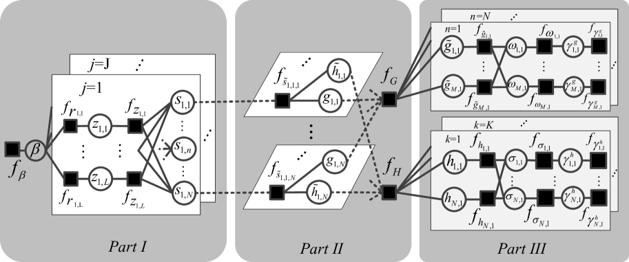
Figure 1: Factor graph representation of (17).

The relationship $\bm{{S}}^{T}=\bm{{H}}^{T}\odot\bm{G}$ in (11) indicates $\bm{\tilde{s}}_{n}=\bm{\tilde{h}}_{n}\otimes\bm{g}_{n}$ with $\bm{{S}}^{T}\triangleq[\bm{\tilde{s}}_{1},\ldots,\bm{\tilde{s}}_{N}]$, $\bm{{H}}^{T}\triangleq[\bm{\tilde{h}}_{1},\ldots,\bm{\tilde{h}}_{N}]$ and $\bm{G}\triangleq[\bm{g}_{1},\ldots,\bm{g}_{N}]$, or in scalar form, i.e, ${\tilde{s}}_{m,k,n}=\tilde{h}_{k,n}{g}_{m,n}$ with $\bm{\tilde{s}}_{n}\triangleq[{\tilde{s}}_{1,1,n},\ldots,{\tilde{s}}_{m,k,n},\ldots,{\tilde{s}}_{M,K,n}]^{T}$, $\bm{\tilde{h}}_{n}\triangleq[\tilde{h}_{1,n},\ldots,\tilde{h}_{K,n}]^{T}$ and $\bm{g}_{n}\triangleq[{g}_{1,n},\ldots,{g}_{M,n}]^{T}$. We next define an auxiliary variable $\bm{\tilde{G}}\triangleq\bm{F}_{1}\bm{\Omega}$ with $\bm{\tilde{G}}\triangleq[\bm{\tilde{g}}_{1},\cdots,\bm{\tilde{g}}_{N}]$ and $\bm{\tilde{g}}_{n}\triangleq[{\tilde{g}}_{1,n},\cdots,{\tilde{g}}_{M,n}]^{T}$. Then, we have the following joint distribution

$$p (\bm{H},\bm{G},\bm{\tilde{G}},\bm{S},\bm{Z},\bm{\Omega},\bm{\Sigma},\bm{\Gamma}^{g},\bm{\Gamma}^{h},\beta|\bm{R})$$

$$= f_{\beta}(\beta){\prod}_{l}{\prod}_{j}\left[f_{{r}_{l,j}}({r}_{l,j},{z}_{l,j},\beta)f_{{z}_{l,j}}({z}_{l,j},\bm{s}_{j})\right]$$

$$~{}\times{\prod}_{m}{\prod}_{n}\Big{[}{\prod}_{k}\left(f_{{\tilde{s}}_{m,k,n}}({\tilde{s}}_{m,k,n},\tilde{h}_{k,n},{g}_{m,n})\right)$$

$$~{}f_{\bm{G}}({{g}}_{m,n},[\bm{\tilde{G}}]_{m,:})f_{{\tilde{g}}_{m,n}}({\tilde{g}}_{m,n},{\omega}_{m,n})f_{{\omega}_{m,n}}({\omega}_{m,n},{\gamma}^{g}_{m,n})$$

$$~{}f_{{\gamma}^{g}_{m,n}}({\gamma}^{g}_{m,n})\Big{]}\times{\prod}_{n}{\prod}_{k}[f_{\bm{H}}(\tilde{h}_{k,n},{{h}}_{n,k})f_{{{h}}_{n,k}}({{h}}_{n,k},{\sigma}_{n,k})$$

$$~{}f_{{\sigma}_{n,k}}({\sigma}_{n,k},{\gamma}^{h}_{n,k})f_{{\gamma}^{h}_{n,k}}({\gamma}^{h}_{n,k})],$$ (17)

where the involved distributions are listed in Table I. The factor graph representation of (17) is depicted in Fig. 1. Based on Fig. 1, we will develop a low-complexity message passing based algorithm to obtain the approximate marginals about the entries of (4) and (7), thereby their estimates.

TABLE I: Factors and distributions in (17).

Factor	Distribution	Function
$f_{\beta}$	$p(\beta)$	$\propto\beta^{-1}$
$f_{{r}_{l,j}}$	$p(\bm{R}|\bm{Z},\beta)$	${\prod}_{l}{\prod}_{j}\mathcal{N}({r}_{l,j};{z}_{l,j},\beta^{-1})$
$f_{{z}_{l,j}}$	$p(\bm{Z}|\bm{S})$	${\prod}_{l}{\prod}_{j}\delta({z}_{l,j}-[\bm{\Psi}]_{l,:}\bm{s}_{j})$
$f_{{\tilde{s}}_{m,k,n}}$	$p(\bm{{S}}|\bm{H},\bm{G})$	${\prod}_{m}{\prod}_{k}{\prod}_{n}\delta({\tilde{s}}_{m,k,n}\!-\!\tilde{h}_{k,n}\otimes{g}_{m,n})$
$f_{\bm{G}}$	$p(\bm{{G}}|\bm{\tilde{G}})$	${\prod}_{m}{\prod}_{n}\delta({{g}}_{m,n}-{[\bm{\tilde{G}}]}_{m,:}{[\bm{F}^{H}_{2}]}_{:,n})$
$f_{{\tilde{g}}_{m,n}}$	$p(\bm{\tilde{G}}|\bm{\Omega})$	${\prod}_{m}{\prod}_{n}\delta({\tilde{g}}_{m,n}-{[\bm{F}_{1}]}_{m,:}{\bm{\omega}}_{n})$
$f_{{\omega}_{m,n}}$	$p(\bm{\Omega}|\bm{\Gamma}^{g})$	${\prod}_{m}{\prod}_{n}\mathcal{N}({\omega}_{m,n};0,(\gamma^{g}_{m,n})^{-1})$
$f_{{\gamma}^{g}_{m,n}}$	$p(\bm{\Gamma}^{g})$	${\prod}_{m}{\prod}_{n}{Ga}(\gamma^{g}_{m,n};\epsilon^{g}_{m,n},\eta^{g}_{m,n})$
$f_{\bm{H}}$	$p(\bm{H}|\bm{{H}}^{T})$	${\prod}_{n}{\prod}_{k}\delta(\tilde{h}_{k,n}-{{h}}_{n,k})$
$f_{{{h}}_{n,k}}$	$p(\bm{{H}}^{T}|\bm{\Sigma})$	${\prod}_{n}{\prod}_{k}\delta({{h}}_{n,k}-{[\bm{F}_{2}]}_{n,:}{\bm{\sigma}}_{k})$
$f_{{\sigma}_{n,k}}$	$p(\bm{\Sigma}|\bm{\Gamma}^{h})$	${\prod}_{n}{\prod}_{k}\mathcal{N}({\sigma}_{n,k};0,(\gamma^{h}_{n,k})^{-1})$
$f_{{\gamma}^{h}_{n,k}}$	$p(\bm{\Gamma}^{h})$	${\prod}_{n}{\prod}_{k}{Ga}(\gamma^{h}_{n,k};\epsilon^{h}_{n,k},\eta^{h}_{n,k})$

IV Message Passing Algorithm Design

As shown in Fig. 1, we divide the factor graph into three parts, and elaborate the message computations in each part.

IV-1 Message Computations in Part $I$

Due to the dense connections in this part and the non-i.i.d. Gaussian entries of matrix $\bm{\Phi}$, UAMP is used to handle the message passing in this part. Here we borrow the algorithm developed in [8]. Due to the space limitation, we do not provide the details, which can be found in [8]. However, it is necessary to illustrate the incoming message $m_{f_{{\tilde{s}}_{m,k,n}}\rightarrow{{s}}_{j,n}}({{s}}_{j,n})$ and outgoing message $m_{{s}_{j,n}\rightarrow f_{\tilde{s}_{m,k,n}}}({s}_{j,n})$.

Part $II$ feeds the incoming message to UAMP as the priori of ${s}_{j,n}$, i.e., $m_{f_{{\tilde{s}}_{m,k,n}}\rightarrow{{s}}_{j,n}}({{s}}_{j,n})=\mathcal{N}(s_{j,n};\overset{\scriptscriptstyle\leftarrow}{s}_{j,n},\overset{\scriptscriptstyle\leftarrow}{\nu}_{{s}_{j,n}})$, where $\overset{\scriptscriptstyle\leftarrow}{\nu}_{{s}_{j,n}}$ and $\overset{\scriptscriptstyle\leftarrow}{s}_{j,n}$ can be respectively updated as

$$\overset{\scriptscriptstyle\leftarrow}{s}_{j,n} =[\overset{\scriptscriptstyle\leftarrow}{\bm{g}}_{n}\cdot\overset{\scriptscriptstyle\leftarrow}{\tilde{\bm{h}}}_{n}]_{j},$$ (18)

$$\overset{\scriptscriptstyle\leftarrow}{\nu}_{{s}_{j,n}}\!\!=\![|\overset{\scriptscriptstyle\leftarrow}{\tilde{\bm{h}}}_{n}|^{2}\cdot\overset{\scriptscriptstyle\leftarrow}{\bm{\nu}}_{\bm{g}_{n}}\!\! +\!|\overset{\scriptscriptstyle\leftarrow}{\bm{g}}_{n}|^{2}\cdot\overset{\scriptscriptstyle\leftarrow}{\bm{\nu}}_{\tilde{\bm{h}}_{n}}\!+\!\overset{\scriptscriptstyle\leftarrow}{\bm{\nu}}_{\tilde{\bm{h}}_{n}}\cdot\overset{\scriptscriptstyle\leftarrow}{\bm{\nu}}_{\bm{g}_{n}}]_{j},$$ (19)

where $\overset{\scriptscriptstyle\leftarrow}{\bm{\nu}}_{\bm{g}_{n}}\triangleq[\overset{\scriptscriptstyle\leftarrow}{\nu}_{g_{1,1,n}},\cdots,\overset{\scriptscriptstyle\leftarrow}{\nu}_{g_{M,K,n}}]^{T}$, $\overset{\scriptscriptstyle\leftarrow}{\bm{g}}_{n}\triangleq[\overset{\scriptscriptstyle\leftarrow}{g}_{1,1,n},\cdots,\overset{\scriptscriptstyle\leftarrow}{g}_{M,K,n}]^{T}$, $\overset{\scriptscriptstyle\leftarrow}{\bm{\nu}}_{\bm{g}_{n}}$, $\overset{\scriptscriptstyle\leftarrow}{\bm{g}}_{n}$, $\overset{\scriptscriptstyle\leftarrow}{\bm{\nu}}_{\tilde{\bm{h}}_{n}}$ and $\overset{\scriptscriptstyle\leftarrow}{\tilde{\bm{h}}}_{n}$ can be computed in the previous iteration. Furthermore, UAMP output the message $m_{{s}_{j,n}\rightarrow f_{\tilde{s}_{m,k,n}}}({s}_{j,n})$ as the input of Part II, i.e.,

$$m_{{s}_{j,n}\rightarrow f_{\tilde{s}_{m,k,n}}}({s}_{j,n})=\mathcal{N}({s}_{j,n};{q}_{j,n},\big{\langle}\sum_{n=1}^{N}{\nu}_{{q}_{j,n}}\big{\rangle}),$$ (20)

where ${q}_{j,n}$ and ${\nu}_{{q}_{j,n}}$ are respectively the $n$-th elements of $\bm{q}_{j}$ and $\bm{\nu}_{\bm{q}_{j}}$ given in the Line 4 of the Algorithm 1 in [8].

IV-2 Message Computations in Part $II$

According to the deterministic relation $\bm{\tilde{G}}=\bm{F}_{1}\bm{\Omega}$, the mean ${g^{\prime}}_{m,n}$ and variance $\nu_{{g^{\prime}}_{m,n}}$ of the Gaussian message $m_{f_{\bm{G}}\rightarrow{g}_{m,n}}({g}_{m,n})$ can be computed as

$$\nu_{g^{\prime}_{m,n}}=\langle\bm{\nu}_{p^{g}_{n}}\rangle,~{}~{}~{}~{}g^{\prime}_{m,n}=[\bm{P}^{g}]_{m,:}[\bm{F}^{H}_{2}]_{:,n},$$ (21)

where $\bm{P}^{g}$ is the corresponding matrix stacked by $\{p^{g}_{m,n}\}$, $\bm{\nu}_{p^{g}_{n}}$ is the vector stacked by $\{\nu_{p^{g}_{m,n}}\}$, $\nu_{p^{g}_{m,n}}$ and $p^{g}_{m,n}$ are respectively the variance and mean of $\tilde{g}_{m,n}$ which will be computed in (39). So the belief of ${g}_{m,n}$ can be expressed as

$$\mathfrak{b}({g}_{m,n}) \propto m_{g_{m,n}\rightarrow f_{{\bm{G}}}}\left(g_{m,n}\right)m_{f_{{\bm{G}}}\rightarrow g_{m,n}}\left(g_{m,n}\right)$$

$$\propto\mathcal{N}(g_{m,n};\hat{g}_{m,n},\nu_{g_{m,n}}),$$ (22)

where the message $m_{g_{m,n}\rightarrow f_{{\bm{G}}}}(g_{m,n})\!=\!\mathcal{N}(g_{m,n};\overset{\scriptscriptstyle\rightarrow}{g}_{m,n},\overset{\scriptscriptstyle\rightarrow}{\nu}_{g_{m,n}})$ can be updated in (29) and (30), and

$$\nu_{{g}_{m,n}}\!\!=\!\overset{\scriptscriptstyle\rightarrow}{\nu}^{-1}_{g_{m,n}}\!\!+\!{\nu}^{-1}_{{g^{\prime}}_{m,n}},~{}~{}~{}~{}\hat{g}_{m,n}\!\!=\!\overset{\scriptscriptstyle\rightarrow}{g}_{m,n}\overset{\scriptscriptstyle\rightarrow}{\nu}^{-1}_{g_{m,n}}\!\!+\!{g^{\prime}}_{m,n}{\nu}^{-1}_{{g^{\prime}}_{m,n}}.$$ (23)

Furthermore, based on the belief propagation, the backward message $m_{{g}_{m,n}\rightarrow f_{{\tilde{s}}_{m,k,n}}}({g}_{m,n})$ can be computed as

$$m_{{g}_{m,n}\rightarrow f_{{\tilde{s}}_{m,k,n}}}({g}_{m,n})=\frac{\mathfrak{b}({g}_{m,n})}{m_{f_{{\tilde{s}}_{m,k,n}}\rightarrow{g}_{m,n}}({g}_{m,n})}.$$ (24)

with variance $\overset{\scriptscriptstyle\leftarrow}{\nu}_{g_{m,k,n}}$ and mean $\overset{\scriptscriptstyle\leftarrow}{g}_{m,k,n}$, which can be computed as

$${\overset{\scriptscriptstyle\leftarrow}{\nu}_{g_{m,k,n}}} =[\bm{\nu}_{\bm{g}_{n}}]_{{mod(mk)}_{K}}^{-1}-\overset{\scriptscriptstyle\rightarrow}{\nu}^{-1}_{g_{m,k,n}},$$ (25)

$${\overset{\scriptscriptstyle\leftarrow}{g}_{m,k,n}} =\overset{\scriptscriptstyle\leftarrow}{\nu}_{g_{m,k,n}}(\hat{g}_{m,n}\nu^{-1}_{{g}_{m,n}}-\overset{\scriptscriptstyle\rightarrow}{g}_{m,k,n}\overset{\scriptscriptstyle\rightarrow}{\nu}^{-1}_{g_{m,k,n}}).$$ (26)

where $mod(i)_{K}$ denotes the $i$-modulo-$K$, $\bm{\nu}_{\bm{g}_{n}}\triangleq[\nu_{{g}_{1,n}},\cdots,\nu_{{g}_{M,n}}]^{T}$, $\overset{\scriptscriptstyle\rightarrow}{\nu}_{g_{m,k,n}}$ and $\overset{\scriptscriptstyle\rightarrow}{g}_{m,k,n}$ will be respectively computed in (27) and (28).

Next, with the definition $[\bm{\tilde{q}}_{1},\cdots,\bm{\tilde{q}}_{N}]\triangleq[\bm{q}_{1},\cdots,\bm{q}_{J}]^{T}$ and $[\bm{\nu}_{\bm{\tilde{q}}_{1}},\cdots,\bm{\nu}_{\bm{\tilde{q}}_{N}}]\triangleq[\bm{\nu}_{{\bm{q}}_{1}},\cdots,\bm{\nu}_{{\bm{q}}_{J}}]^{T}$, mean field rules [9, 10] indicate that the forward message $m_{f_{\tilde{s}_{m,k,n}}\rightarrow g_{m,n}}(g_{m,n})\propto\mathcal{N}(g_{m,n};\overset{\scriptscriptstyle\rightarrow}{g}_{m,k,n},\overset{\scriptscriptstyle\rightarrow}{\nu}_{g_{m,k,n}})$ with

$$\overset{\scriptscriptstyle\rightarrow}{\nu}_{g_{m,k,n}} =\langle\bm{\nu}_{\bm{\tilde{q}}_{k,n}}\rangle({|\hat{\tilde{h}}_{k,n}|^{2}+\nu_{\tilde{h}_{k,n}}})^{-1},$$ (27)

$$\overset{\scriptscriptstyle\rightarrow}{g}_{m,k,n} ={\tilde{q}_{m,k,n}\hat{\tilde{h}}_{k,n}^{*}}({|\hat{\tilde{h}}_{k,n}|^{2}+\nu_{\tilde{h}_{k,n}}})^{-1},$$ (28)

where $\hat{\tilde{h}}_{k,n}$ and $\nu_{\tilde{h}_{k,n}}$ are the approximated a posteriori mean and variance of ${\tilde{h}}_{k,n}$, which are computed in the previous iteration, $\bm{\nu}_{\bm{\tilde{q}}_{k,n}}$ is the $k$-th block of $\bm{\nu}_{\bm{\tilde{q}}_{n}}\triangleq[\bm{\nu}_{\bm{\tilde{q}}_{1,n}}^{T},\cdots,\bm{\nu}_{\bm{\tilde{q}}_{K,n}}^{T}]^{T}$, ${\bm{\tilde{q}}_{n}}\triangleq[{\bm{\tilde{q}}_{1,n}}^{T},\cdots,{\bm{\tilde{q}}_{K,n}}^{T}]^{T}$, and $\tilde{q}_{m,k,n}$ is the $m$-th element of ${\bm{\tilde{q}}_{k,n}}$, i.e., ${\bm{\tilde{q}}_{k,n}}\triangleq[\tilde{q}_{1,k,n},\cdots,\tilde{q}_{M,k,n}]^{T}$. With belief propagation rules, we have $m_{g_{m,n}\rightarrow f_{{\bm{G}}}}(g_{m,n})\!=\!\mathcal{N}(g_{m,n};\overset{\scriptscriptstyle\rightarrow}{g}_{m,n},\overset{\scriptscriptstyle\rightarrow}{\nu}_{g_{m,n}})$ with

$$\overset{\scriptscriptstyle\rightarrow}{\nu}_{g_{m,n}} =(\sum_{k=1}^{K}\overset{\scriptscriptstyle\rightarrow}{\nu}^{-1}_{g_{m,k,n}})^{-1},$$ (29)

$$\overset{\scriptscriptstyle\rightarrow}{g}_{m,n} =\overset{\scriptscriptstyle\rightarrow}{\nu}_{g_{m,n}}\sum_{k=1}^{K}\!{\overset{\scriptscriptstyle\rightarrow}{g}_{m,k,n}}{\overset{\scriptscriptstyle\rightarrow}{\nu}^{-1}_{g_{m,k,n}}}.$$ (30)

Then, we have the message $m_{f_{\bm{G}}\rightarrow{\tilde{g}}_{m,n}}(\tilde{g}_{m,n})=\mathcal{N}(\tilde{g}_{m,n};\overset{\scriptscriptstyle\rightarrow}{\tilde{g}}_{m,n},\overset{\scriptscriptstyle\rightarrow}{\nu}_{\tilde{g}_{m,n}})$ with

$$\overset{\scriptscriptstyle\rightarrow}{\nu}_{\tilde{g}_{m,n}}=\frac{1}{N}\sum\nolimits_{n=1}^{N}\overset{\scriptscriptstyle\rightarrow}{\nu}_{g_{m,n}}^{-1},~{}~{}~{}~{}~{}\overset{\scriptscriptstyle\rightarrow}{\tilde{g}}_{m,n}=[\overset{\scriptscriptstyle\rightarrow}{\bm{G}}]_{m,:}[{\bm{F}_{2}}]_{:,n},$$ (31)

where $\overset{\scriptscriptstyle\rightarrow}{\bm{G}}$ is the corresponding matrix stacked by $\overset{\scriptscriptstyle\rightarrow}{\nu}_{g_{m,n}}$.

Because of the symmetry between $\{\tilde{h}_{k,n}\}$ and $\{g_{m,n}\}$, the forward and backward messages related to $\{\tilde{h}_{k,n}\}$ in this part can be reached following the same steps from (21) and (31) by replacing the corresponding parameters, except for the following means and variables.

$$\nu_{{h}^{{}^{\prime}}_{k,n}}=\nu_{p^{h}_{n,k}},~{}~{}~{}~{}{{h}^{\prime}}_{k,n}=p^{h}_{n,k},$$ (32)

$$\overset{\scriptscriptstyle\rightarrow}{\nu}_{{h}_{n,k}}=\overset{\scriptscriptstyle\rightarrow}{\nu}_{\tilde{h}_{k,n}},~{}~{}~{}~{}~{}\overset{\scriptscriptstyle\rightarrow}{{h}}_{n,k}=\overset{\scriptscriptstyle\rightarrow}{\tilde{h}}_{k,n}.$$ (33)

Then, we treat $m_{f_{\bm{G}}\rightarrow{\tilde{g}}_{m,n}}(\tilde{g}_{m,n})$ and $m_{f_{\bm{H}}\rightarrow{\tilde{h}}_{n,k}}(\tilde{h}_{n,k})$ as the inputs of the Part $III$.

IV-3 Message Computations in Part $III$

We first elaborate the backward message passing. The message $m_{f_{\gamma^{g}_{m,n}}\rightarrow\gamma^{g}_{m,n}}(\gamma^{g}_{m,n})$ is predefined Gamma distribution with shape parameter $\epsilon^{g}_{m,n}$ and rate parameter $\eta^{g}_{m,n}$, i.e.,

$$m_{f_{\gamma^{g}_{m,n}}\!\!\rightarrow\gamma^{g}_{m,n}}(\gamma^{g}_{m,n})\!\propto\!(\gamma^{g}_{m,n})^{\epsilon^{g}_{m,n}\!-\!1}\!\exp\left\{-\eta^{g}_{m,n}\gamma^{g}_{m,n}\right\}.$$ (34)

So $\mathfrak{b}({\gamma}^{g}_{m,n})\propto m_{f_{{\gamma}^{g}_{m,n}}\rightarrow{\gamma}^{g}_{m,n}}({\gamma}^{g}_{m,n})m_{f_{{\omega}_{m,n}}\rightarrow{\gamma}^{g}_{m,n}}({\gamma}^{g}_{m,n})$. Then $\hat{\gamma}^{g}_{m,n}$ can be computed as

$$\hat{\gamma}^{g}_{m,n}\!\!=\!\!\int\!\!\gamma^{g}_{m,n}\mathfrak{b}\left(\gamma^{g}_{m,n}\right)d\gamma^{g}_{m,n}\!\!=\!\!\frac{2\epsilon^{g}_{n}\!\!+\!1}{|\hat{\omega}_{m,n}|^{2}\!\!+\!\nu_{\omega_{m,n}}\!\!+\!2{\eta}^{g}_{m,n}},$$ (35)

where $\hat{{\omega}}_{m,n}$ and ${\nu}_{{\omega}_{m,n}}$ are given in (44), and the shape parameter is tuned automatically using the rule in [11]

$$\epsilon^{g}_{n}=0.5\sqrt{{\log({M^{-1}}\!\sum\nolimits_{m}\hat{\gamma}^{g}_{m,n})\!-\!{M^{-1}}\!\log\sum\nolimits_{m}\hat{\gamma}^{g}_{m,n}}}.$$ (36)

Then, it holds that

$$m_{f_{\omega_{m,n}}\rightarrow\omega_{m,n}}(\omega_{m,n})\propto\mathcal{N}(\omega_{m,n};0,(\hat{\gamma}^{g}_{m,n})^{-1}).$$ (37)

We then sent $m_{f_{\omega_{m,n}}\rightarrow\omega_{m,n}}(\omega_{m,n})$ to UAMP as the prior of $\omega_{m,n}$, and UAMP outputs the Gaussian messages $m_{\tilde{g}_{m,n}\rightarrow f_{\bm{{G}}}}(\tilde{g}_{m,n})=m_{f_{\tilde{g}_{m,n}}\rightarrow{\tilde{g}_{m,n}}}\!(\tilde{g}_{m,n})$, i.e.,

$${m_{\tilde{g}_{m,n}\rightarrow f_{\bm{{G}}}}\!(\tilde{g}_{m,n})\!\!=\mathcal{N}(\tilde{g}_{m,n};p^{g}_{m,n},\nu_{p^{g}_{m,n}})},$$ (38)

where $\nu_{p^{g}_{m,n}}$ and $p^{g}_{m,n}$ are updated as

$$\nu_{p^{g}_{m,n}} =\big{\langle}{\sum_{m=1}^{M}{\nu}_{\omega_{m,n}}}\big{\rangle},~{}~{}{p^{g}_{m,n}}\!\!=\!\![\bm{F}_{1}]_{m,:}\hat{\bm{\omega}}_{n}\!\!-\!\nu_{p^{g}_{m,n}}\mu^{g}_{m,n},$$ (39)

and $\hat{\bm{\omega}}_{n}\triangleq[\hat{{\omega}}_{1,n},\cdots,\hat{{\omega}}_{M,n}]^{T}$, $\mu^{g}_{m,n}$ can be obtained by (42), $\hat{{\omega}}_{m,n}$ and ${\nu}_{{\omega}_{m,n}}$ denote the available mean and variance, respectively, which are given in (44).

Next, in the forward direction, based on the message $m_{f_{\bm{G}}\rightarrow{\tilde{g}}_{m,n}}(\tilde{g}_{m,n})$, we first apply UAMP in Part $III$ where the intensive connections exists. Specifically, UAMP suggests that the message from function node $\omega_{m,n}$ to variable node $f_{\omega_{m,n}}$ is

$$m_{\omega_{m,n}\rightarrow f_{{\omega}_{m,n}}}(\omega_{m,n})\propto\mathcal{N}(\omega_{m,n};q^{g}_{m,n},\nu_{q^{g}_{m,n}}),$$ (40)

with mean $q^{g}_{m,n}$ and variance $\nu_{q^{g}_{m,n}}$, which are given by

$${\nu}_{q^{g}_{m,n}}=1/\langle\bm{\nu}_{\bm{\mu}^{g}_{n}}\rangle,~{}~{}~{}~{}~{}{{q}^{g}_{m,n}}\!\!=\!\hat{\omega}_{m,n}\!\!+\!{\nu}_{q^{g}_{m,n}}[\bm{F}_{1}]_{m,:}{\bm{\mu}^{g}_{n}},$$ (41)

where $\bm{\nu}_{\bm{\mu}^{g}_{n}}$ and ${\bm{\mu}^{g}_{n}}$ are respectively the vector-form of ${\nu}_{\mu^{g}_{m,n}}$ and $\mu^{g}_{m,n}$, which is given by

$${\nu}_{\mu^{g}_{m,n}}\!\! =\!\!{1}/({\nu}_{p^{g}_{m,n}}\!\!+\!\overset{\scriptscriptstyle\rightarrow}{\nu}_{\tilde{g}_{m,n}}),~{}\mu^{g}_{m,n}\!\!=\!\!{\nu}_{\mu^{g}_{m,n}}(\overset{\scriptscriptstyle\rightarrow}{\nu}_{\tilde{g}_{m,n}}\!\!-\!{p}^{g}_{m,n}).$$ (42)

Then, variational message passing is adopted to compute the message

$$m_{f_{\omega_{m,n}}\rightarrow{{\gamma}^{g}_{m,n}}}\!({{\gamma}^{g}_{m,n}})$$

$$\propto\exp\left\{\int\mathfrak{b}(\omega_{m,n})\log f_{\omega_{m,n}}(\omega_{m,n})d{\omega_{m,n}}\right\},$$ (43)

where $\mathfrak{b}(\omega_{m,n})\propto m_{{\omega_{m,n}}\rightarrow f_{\omega_{m,n}}}({\omega_{m,n}})m_{f_{\omega_{m,n}}\rightarrow{\omega_{m,n}}}({\omega_{m,n}})$. As a multiplication of several Gaussian functions, $\mathfrak{b}\left({\omega}_{m,n}\right)$ is still Gaussian, i.e., $\mathfrak{b}\left({\omega}_{m,n}\right)\propto\mathcal{N}(\omega_{m,n};\hat{\omega}_{m,n},\nu_{\omega_{m,n}})$ with

$$\nu_{\omega_{m,n}}=\frac{{\nu}_{q^{g}_{m,n}}}{1+{\nu}_{q^{g}_{m,n}}\hat{\gamma}^{g}_{m,n}},~{}~{}~{}~{}\hat{\omega}_{m,n}=\frac{q^{g}_{m,n}}{1+{\nu}_{q^{g}_{m,n}}\hat{\gamma}^{g}_{m,n}}.$$ (44)

Then, according to the above, we have

$$m_{f_{\omega_{m,n}}\!\rightarrow{{\gamma}^{g}_{m,n}}}({{\gamma}^{g}_{m,n}})\!\propto\!\exp\big{\{}\!\!-\!\!\frac{{\gamma}^{g}_{m,n}}{2}(|\hat{\omega}_{m,n}|^{2}\!\!+\!\nu_{\omega_{m,n}})\big{\}}.$$ (45)

As shown in the Part $III$ of Fig. 1, due to the symmetry between $\{\omega_{m,n}\}$ and $\{\sigma_{n,k}\}$, we can directly obtain the messages about $\{\sigma_{n,k}\}$ by replacing the corresponding parameters.

The proposed algorithm is summarized in Algorithm 1. The complexity of Part $I$ and $II$ is $\mathcal{O}(NLKM)$, and the complexity involved in Part $III$ is $\mathcal{O}(NK\log_{2}{N})$ or $\mathcal{O}(NM\log_{2}{M})$ thanks to the FFT in (39) and (41). The complexity is lower than that of the channel estimation method in [5], which is $\mathcal{O}(N^{2}M^{2})$.

Algorithm 1 The proposed algorithm

Input: $\bm{\Phi}$, $\zeta$ and the maximum number of iteration $I_{max}$.
Initialize: $\hat{\omega}_{m,n}\!=\!0,\nu_{{\omega}_{m,n}}\!=\!1,{s}^{g}_{m,n}\!=\!0,\hat{\gamma}^{g}_{m,n}\!=\!1,\epsilon^{g}_{n}\!=\!0.001,\hat{\sigma}_{n,k}\!=\!0,\nu_{{\sigma}_{n,k}}\!=\!1,{s}^{h}_{n,k}\!=\!0,\hat{\gamma}^{h}_{n,k}\!=\!1,\epsilon^{h}_{k}\!=\!0.001$, $\forall m,k,n,j$.
Repeat:

1:  $\forall j$: update $\bm{q}_{j}$ and $\bm{\nu}_{\bm{q}_{j}}$ as the Line 4 of the Algorithm 1 in [8]

2:  $\forall m,k,n$: update $\overset{\scriptscriptstyle\rightarrow}{\nu}_{g_{m,k,n}}$, $\overset{\scriptscriptstyle\rightarrow}{g}_{m,k,n}$ with (27), (28);

3:  $\forall m,n$: update $\overset{\scriptscriptstyle\rightarrow}{\nu}_{g_{m,n}}$, $\overset{\scriptscriptstyle\rightarrow}{g}_{m,n}$, $\overset{\scriptscriptstyle\rightarrow}{\nu}_{\tilde{g}_{m,n}}$, $\overset{\scriptscriptstyle\rightarrow}{\tilde{g}}_{m,n}$ with (29), (30), (31);

4:  $\forall m,n$: update ${\nu}_{\mu^{g}_{m,n}},{\mu^{g}_{m,n}},{\nu}_{q^{g}_{m,n}},{q^{g}_{m,n}}$, $\nu_{\omega_{m,n}}$, $\hat{\omega}_{m,n}$, $\hat{\gamma}^{g}_{m,n}$ with (42), (41), (44), (35);

5:  $\forall n$: update ${\epsilon}^{g}_{n}$ with (36);

6:  $\forall m,n$: update ${\nu}_{p^{g}_{m,n}},{p^{g}_{m,n}},{\nu}_{g^{\prime}_{m,n}},{g^{\prime}_{m,n}}$, $\nu_{g_{m,n}}$, $\hat{g}_{m,n}$, $\overset{\scriptscriptstyle\leftarrow}{\nu}_{g_{m,n}}$, $\overset{\scriptscriptstyle\leftarrow}{g}_{m,n}$ with (39), (21), (23) and the Line 15 of Algorithm 1 in [8];

7:  $\forall k,n$: repeat step 2 to step 6 after replacing the corresponding parameters related to $\{\tilde{h}_{k,n}\}$ and $\{\sigma_{n,k}\}$;

8:  $\forall j,n$: update $\overset{\scriptscriptstyle\leftarrow}{\nu}_{{s}_{j,n}}$, $\overset{\scriptscriptstyle\leftarrow}{s}_{j,n}$ with 19 and 18;

Until $\frac{\sum_{m,n}|\hat{\omega}_{m,n}-{\omega}_{m,n}|^{2}}{\sum_{m,n}|{\omega}_{m,n}|^{2}}<\zeta$ and $\frac{\sum_{k,n}|\hat{\sigma}_{n,k}-{\sigma}_{n,k}|^{2}}{\sum_{k,n}|{\sigma}_{n,k}|^{2}}<\zeta$ or the number of iteration is more than $I_{max}$.
Output: $\hat{\omega}_{m,n}$, $\hat{\sigma}_{n,k}$.

V Simulation Results

In this section, we provide numerical experiments to demonstrate the superior performance of the proposed message passing algorithm. The most relevant work for comparison is [5], where a matrix-Calibration-based (MCB) channel estimation algorithm is proposed. In addition, we also include the performance of the oracle least-square (LS) estimator as a bound, which assumes the knowledge of the support of the sparse channels. It is noted that there exists an inevitable scaling ambiguity in the channel estimation, which is removed in the calculation of the normalized mean square error (NMSE). In our simulations, we set $M=K=N=32$, $N_{1}=4$ and $N_{2}=8$. The RIS phase matrix $\bm{\Phi}$ is selected as a partial DFT matrix. We assume a Rician channel comprising a line-of-sight path and a number of non line-of-sight paths and the Rician factor is set to 13.2dB [1]. The number of paths for mmWave channels $\bm{G}$ and $\bm{h}_{k}$ are respectively set to $P=3$ and $P^{\prime}=3$, where the AoA and AoD parameters are uniformly generated from $[-\pi/2,\pi/2]$ and not necessarily lie on the discretized grid. The threshold $\zeta=\!10^{-3}$ and $I_{max}=30$.

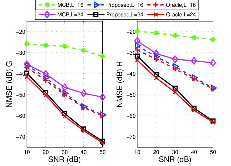
Figure 2: NMSE performance of the estimators versus SNR.

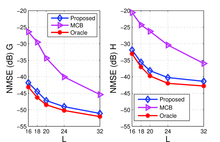
Figure 3: NMSE performance of the estimators versus SNR for different $L$.

In Fig. 2, we compare the NMSE performance versus SNR of the estimators with different values of $L$. As shown by the results, the proposed method performs significantly better than the MCB method, especially when $L$ is relatively small. It is noted that a smaller $L$ (the number of RIS phase configurations needed for channel estimation) is highly desirable to reduce the training overhead and latency. The results also show that the proposed method can achieve performance close to that of the oracle LS estimator for different $L$, even for small $L$. Next, we vary the value of $L$ and examine the performance of the estimators in Fig. 3, where the SNR is set to 20dB. It can be seen that the performances of all estimators improve as expected with $L$. To achieve the same MSE performance, the proposed algorithm uses significantly smaller $L$, indicating that the overhead and latency due to the channel estimation are greatly reduced.

References

• [1] P.ย Wang, J.ย Fang, H.ย Duan, and H.ย Li, โ€œCompressed channel estimation for intelligent reflecting surface-assisted millimeter wave systems,โ€ IEEE Signal Processing Lett., vol.ย 27, pp. 905โ€“909, 2020.
• [2] C.ย Huang, A.ย Zappone, G.ย C. Alexandropoulos, M.ย Debbah, and C.ย Yuen, โ€œReconfigurable intelligent surfaces for energy efficiency in wireless communication,โ€ IEEE Trans. Wireless Commun., vol.ย 18, no.ย 8, pp. 4157โ€“4170, 2019.
• [3] Z.ย Peng, G.ย Zhou, C.ย Pan, H.ย Ren, A.ย L. Swindlehurst, P.ย Popovski, and G.ย Wu, โ€œChannel estimation for RIS-aided multi-user mmWave systems with uniform planar arrays,โ€ IEEE Trans. Commun., vol.ย 70, no.ย 12, pp. 8105โ€“8122, 2022.
• [4] Z.-Q. He and X.ย Yuan, โ€œCascaded channel estimation for large intelligent metasurface assisted massive MIMO,โ€ IEEE Wireless Commun. Lett., vol.ย 9, no.ย 2, pp. 210โ€“214, 2020.
• [5] H.ย Liu, X.ย Yuan, and Y.-J.ย A. Zhang, โ€œMatrix-calibration-based cascaded channel estimation for reconfigurable intelligent surface assisted multiuser MIMO,โ€ IEEE J. Sel. Areas Commun., vol.ย 38, no.ย 11, pp. 2621โ€“2636, 2020.
• [6] Z.ย Wang, L.ย Liu, and S.ย Cui, โ€œChannel estimation for intelligent reflecting surface assisted multiuser communicationsโ€… Framework, algorithms, and analysis,โ€ IEEE Trans. Wireless Commun., vol.ย 19, no.ย 10, pp. 6607โ€“6620, 2020.
• [7] X.ย Zhang, X.ย Shao, Y.ย Guo, Y.ย Lu, and L.ย Cheng, โ€œSparsity-structured tensor-aided channel estimation for RIS-assisted MIMO communications,โ€ IEEE Commun. Lett., vol.ย 26, no.ย 10, pp. 2460โ€“2464, 2022.
• [8] Y.ย Guo, P.ย Sun, Z.ย Yuan, C.ย Huang, Q.ย Guo, Z.ย Wang, and C.ย Yuen, โ€œEfficient channel estimation for RIS-aided MIMO communications with unitary approximate message passing,โ€ IEEE Trans. Wireless Commun., vol.ย 22, no.ย 2, pp. 1403โ€“1416, 2023.
• [9] Q.ย Guo and J.ย Xi, โ€œApproximate message passing with unitary transformation,โ€ CoRR, vol. abs/1504.04799, 2015. [Online]. Available: http://arxiv.org/abs/1504.04799
• [10] Z.ย Yuan, Q.ย Guo, and M.ย Luo, โ€œApproximate message passing with unitary transformation for robust bilinear recovery,โ€ IEEE Trans. Signal Processing, vol.ย 69, pp. 617โ€“630, 2021.
• [11] M.ย Luo, Q.ย Guo, M.ย Jin, Y.ย C. Eldar, D.ย Huang, and X.ย Meng, โ€œUnitary approximate message passing for sparse bayesian learning,โ€ IEEE Trans. Signal Process., vol.ย 69, pp. 6023โ€“6039, 2021.