Liouville soliton surfaces obtained using Darboux transformations

Abstract

In this paper, Liouville soliton surfaces based on some soliton solutions of the Liouville equation are constructed and displayed graphically, including some of those corresponding to Darboux-transformed counterparts. We find that the Liouville soliton surfaces are centroaffine surfaces of Tzitzeica type and their centroaffine invariant can be expressed in terms of the Hamiltonian. The traveling wave solutions to Liouville equation from which these soliton surfaces stem are also obtained through a modified variation of parameters method which is shown to lead to elliptic functions solution method.

Keywords: Liouville equation, Liouville soliton surface, centro-affine invariant, Darboux transformation, Lax pair.

Physica Scripta 98, 075227 (2023)

I Introduction

In this paper, we introduce soliton surfaces based on the Liouville sech² soliton solution and also of its Darboux/auto-Bäcklund transformations. The employed Liouville soliton is one of the common solutions obtained by using linear arbitrary functions $\Phi(u)$ and $\Psi(v)$ in the Liouville representation of the general solution. Although the Darboux/auto-Bäcklund transformations are known for more than a century in mathematics, and the concept of soliton surface has been introduced in mathematical physics in the 1980s sym83 ; sym85 , we could not find any discussion of the Liouville soliton surfaces in the recent literature, e.g., cies98 ; gp12 ; gpr14 . This gap in the literature served us as a motivation for writing this paper. Another motivation is that soliton surfaces are geometrical analogs of gauge theories of (super)strings, spin systems, and chiral integrable models of elementary particles in which the interaction is not generated by considering interaction Lagrangians, but has pure geometric origin related to the curvature of the soliton surface and other geometric and topological concepts sym83 ; sym85 ; perel87 ; dt07 .

This paper is structured as follows. In Section 2, some very basic results about the Liouville equation with some historical flavor are provided. In Section 3, the affine geometric representation is described following methods originally due to Tzitzeica. It is shown that the Liouville soliton surfaces are centroaffine surfaces and their centroaffine invariant is the Hamiltonian. In Section 4, a modified variation of parameters method is shown to be of usage in obtaining the same Liouville soliton solution providing also a direct way to the Hamiltonian of the system. In section 5, the Lax pair of matrices introduced by Mikhaĭlov Mikh are used to obtain the coordinates of the soliton surfaces in the case of Darboux-transformed solutions and two such surfaces obtained in this way are displayed graphically. A concluding section summarizes the results and presents some perspectives for possible future work.

II The Liouville equation: A brief historical sketch

The Liouville nonlinear equation first occurred around 1850 as a result obtained by Liouville when he carefully studied the surfaces of constant curvature, cf. one of his notes, in the fifth edition of the famous textbook by Monge mo curated by Liouville. He was led to the following partial differential equation

$${(\log\lambda)}_{uv}\pm\frac{\lambda}{2a^{2}}=0~{},$$ (1)

where $a$ is a real arbitrary constant. By letting $\alpha=\mp\frac{1}{2a^{2}}$, and denoting $\Lambda=\log\lambda$, this equation may be written in the equivalent form

$$E(\Lambda)\equiv\Lambda_{uv}-\alpha e^{\Lambda}=0~{}.$$ (2)

In his notes, Liouville presented a very simple method to the complete integral of (1) through some geometric considerations related to the properties of the sphere mo ; Lio . His solution, involving two arbitrary functions $\Phi(u)$ and $\Psi(v)$ was written as

$$\lambda(u,v)=\frac{2}{\mp\alpha}\frac{\Phi_{u}\Psi_{v}~{}e^{\Phi(u)+\Psi(v)}}{[1\pm e^{\Phi(u)+\Psi(v)}]^{2}}~{}.$$ (3)

One can easily see that (3) can be also written as

$$\begin{array}[]{l}\lambda(u,v)=\mp\frac{1}{2\alpha}\Phi_{u}\Psi_{v}{\rm sech}^{2}\left(\frac{\Phi(u)+\Psi(v)}{2}\right)~{}\quad{\rm or}\\ \lambda(u,v)=\pm\frac{1}{2\alpha}\Phi_{u}\Psi_{v}{\rm cosech}^{2}\left(\frac{\Phi(u)+\Psi(v)}{2}\right)~{},\end{array}$$ (4)

corresponding to bound and singular at the origin solutions, respectively. An even simpler form of (3) can be obtained by using the substitutions $\log\phi=\Phi$, and $\log\psi=\Psi$,

$$\lambda(u,v)=\frac{2}{\mp\alpha}\frac{\phi_{u}\psi_{v}}{\left(1\pm\phi\psi\right)^{2}}~{}.$$ (5)

The Liouville equation stayed nearly dormant for more than a century until its application as a key dynamical equation of motion for the string degrees of freedom in quantum field theory, two-dimensional gravity, and soliton particle physics models has been revealed during the decade 1980. We recommend the reader the reviews bn ; teschner . Interestingly, it has been found that some singular Liouville solutions may play a role in the relativistic string dynamics since they do no make the string singular and consequently their mathematics has been further developed in dpp ; jkm .

III An affine surface and the Bäcklund Transformation

It was noted by the Romanian mathematician Gheorghe Titeica, a.k.a. Georges Tzitzéica TG who studied under Darboux and Goursat, that in some asymptotic coordinates $u,v$, surfaces $\Sigma$ parametrized by $s^{1}(u,v),~{}s^{2}(u,v),~{}s^{3}(u,v)$ have the property that the Gaussian curvature ${\cal K}$ is proportional to the fourth power of the distance $D$ from the origin $O$ to the tangent plane to the surface $\Sigma$ at some point $P$ of coordinates $(s^{1},s^{2},s^{3})$. Thus, Tzitzéica introduced the centroaffine constant invariant ${\cal I}$ defined by

$${\cal I}=\frac{{\cal K}}{D^{4}}~{}.$$ (6)

The idea to construct surfaces in this way was also used by Tzitzéica for the equation rediscovered by Dodd and Bullough (the Dodd-Bullough equation), and further he introduced a mapping (auto-Bäcklund transformation) between surfaces in his papers TG1 ; TG2 , and book published in French TG .

These surfaces therefore admit the affine representation given by the coordinates $(s^{1},s^{2},s^{3})$ which are three linearly independent integrals of the linear system

$$\begin{array}[]{ll}&s_{uu}=as_{u}+bs_{v}~{},\\ &s_{uv}=\alpha\lambda s~{},\\ &s_{vv}=a^{\prime}s_{u}+b^{\prime}s_{v}~{}.\end{array}$$ (10)

For the specific values of $a=\frac{\lambda_{u}}{\lambda}$, $b=a^{\prime}=0$, and $b^{\prime}=\frac{\lambda_{v}}{\lambda}$, any solution $\lambda(u,v)$ of the Liouville equation represents the compatibility solution of the system

$$\begin{array}[]{ll}&s_{uu}=\frac{\lambda_{u}}{\lambda}s_{u}~{},\\ &s_{uv}=\alpha\lambda s~{},\\ &s_{vv}=\frac{\lambda_{v}}{\lambda}s_{v}~{}.\end{array}$$ (14)

The first Lax pair for (2), known by Tzitzéica, is given by

$$\begin{array}[]{l}S_{u}=LS\\ S_{v}=AS\end{array}~{},$$ (15)

where $S(u,v)$ is a vector valued wave function given by $S^{T}=(s_{v},s_{u},s)$, and $L$, $A$ are the third order matrices

$$L=\begin{pmatrix}0&0&\alpha e^{\Lambda}\\ 0&\Lambda_{u}&0\\ 0&1&0\end{pmatrix},\,\,\,\,\,\,\,A=\begin{pmatrix}\Lambda_{v}&0&0\\ 0&0&\alpha e^{\Lambda}\\ 1&0&0\end{pmatrix}.$$ (16)

This pair satisfies the compatibility condition $S_{uv}=S_{vu}$ which leads to

$$L_{v}-A_{u}+[L,A]=\begin{pmatrix}-E(\Lambda)&0&0\\ 0&E(\Lambda)&0\\ 0&0&0\end{pmatrix}.$$ (17)

We are interested in generating solitonic surfaces corresponding to (1) and first Lax pair (16) for which we use a linear form of the general functions given by

$$\begin{array}[]{l}\Phi(u)=2\sqrt{\alpha}~{}ku~{},\\ \Psi(v)=-2\sqrt{\alpha}~{}\omega v~{}.\end{array}$$ (18)

Since we deal with solitons, we also use henceforth the right- and left-moving traveling coordinates, $\xi=ku-\omega v$ and $\zeta=ku+\omega v$, respectively, and also known as light-cone coordinates in the context of linear wave equations. Thus, for $\alpha>0$, the soliton solution of (1) in the variable $\xi$ has the form,

$$\lambda(u,v)=2k\omega~{}\mathrm{sech}^{2}\left(\sqrt{\alpha}\xi\right)~{}.$$ (19)

This will be the seed solution used to generate $\Sigma$. To find the surface corresponding to these solutions, we need to solve the linear system (14). By two quadratures the third equation leads to

$$s(u,v)=-c_{1}(u)\frac{\tanh\left(\sqrt{\alpha}\xi\right)}{\sqrt{\alpha}\omega}+c_{2}(u)=\left[-\frac{c_{1}(u)}{\sqrt{\alpha}\omega}\sinh\left(\sqrt{\alpha}\xi\right)+c_{2}(u)\cosh\left(\sqrt{\alpha}\xi\right)\right]\text{sech}\left(\sqrt{\alpha}\xi\right)~{},$$ (20)

while the second equation is satisfied for

$$c_{2}(u)=\frac{c_{1}(u)^{\prime}}{2k\alpha\omega}~{}.$$ (21)

To find $c_{1}(u)$ we substitute the last two in the first equation of (14), which leads to the third order linear differential equation

$$c_{1}(u)^{\prime\prime\prime}-4\alpha k^{2}c_{1}(u)^{\prime}=0~{}.$$ (22)

Thus, the surface $\Sigma$ is determined by the algebraic curves of the cubic

$$m^{3}-4\alpha k^{2}m=0$$ (23)

with roots $m_{1}=0$, $m_{2,3}=\pm 2\sqrt{\alpha}k$ which lead to the three solutions

$$\begin{array}[]{ll}&c_{1}^{1}(u)=\sqrt{\alpha}\omega~{},\\ &c_{1}^{2}(u)=\sqrt{\alpha}\omega\sinh(2\sqrt{\alpha}k~{}u)~{},\\ &c_{1}^{3}(u)=\sqrt{\alpha}\omega\cosh(2\sqrt{\alpha}k~{}u)~{}.\end{array}$$ (27)

Using these functions in (21) and (20), the three linearly independent solutions of system (14)

$$\begin{array}[]{ll}&s^{1}(u,v)=\mathrm{sinh}\left(\sqrt{\alpha}\xi\right)\mathrm{sech}\left(\sqrt{\alpha}\xi\right)~{},\\ &s^{2}(u,v)=\cosh\left(\sqrt{\alpha}\zeta\right)~{}\mathrm{sech}\left(\sqrt{\alpha}\xi\right)~{},\\ &s^{3}(u,v)=\mathrm{sinh}\left(\sqrt{\alpha}\zeta\right)~{}\mathrm{sech}\left(\sqrt{\alpha}\xi\right)~{}.\\ \end{array}$$ (31)

The Darboux-transformed Liouville solutions can be successively generated using the invariant transformations Bre , Schief

$$\tilde{\lambda}^{i}=-\lambda+\frac{2}{\alpha}(\log s^{i})_{u}(\log s^{i})_{v}~{},$$ (32)

where $\lambda$ is the seed solution given by (19), and $s^{i}$ with $i=1,2,3$, is any solution of (31). This type of transformation known as Bäcklund transformation represents a relation between two sets of independent solutions $\lambda$ and $\tilde{\lambda}$ of the same PDE.

Using successively these three solutions, the new potentials $\tilde{\lambda}$ are

$$\begin{array}[]{ll}&\tilde{\lambda}^{1}(u,v)=-2k\omega~{}\mathrm{csch}^{2}\left(\sqrt{\alpha}\xi\right)~{},\\ &\tilde{\lambda}^{2}(u,v)=-2k\omega~{}\mathrm{sech}^{2}\left(\sqrt{\alpha}\zeta\right)~{},\\ &\tilde{\lambda}^{3}(u,v)=2k\omega~{}\mathrm{csch}^{2}\left(\sqrt{\alpha}\zeta\right)~{}.\\ \end{array}$$ (36)

These are also solutions to the Liouville equation (1), and can be infinitely many times generated using (32).

The three solutions $s^{i}(u,v)$ allow us to generate a parametric surface $\Sigma(s^{1},s^{2},s^{3})$ in $\mathbb{R}^{3}$ known as the Liouville soliton surface. To classify the surface, notice the quadratic relation between these solutions defining the one-sheeted hyperboloid

$$\Sigma(u,v)\equiv[s^{1}(u,v)]^{2}+[s^{2}(u,v)]^{2}-[s^{3}(u,v)]^{2}=\frac{4k^{2}}{\alpha}~{},$$ (37)

for which

$$s^{3}=h(s^{1},s^{2})=\sqrt{[s^{1}(u,v)]^{2}+[s^{2}(u,v)]^{2}-\frac{4k^{2}}{\alpha}}~{}.$$ (38)

To calculate the centroaffine invariant for this surface, we use the curvature

$${\cal K}=\frac{|h_{s^{1}s^{1}}h_{s^{2}s^{2}}-(h_{s^{1}s^{2}})^{2}|}{\left[1+(h_{s^{1}})^{2}+(h_{s^{2}})^{2}\right]^{2}}~{},$$ (39)

and distance $D$

$$D=\frac{|s^{1}h_{s^{1}}+s^{2}h_{s^{2}}-h(s^{1},s^{2})|}{\left[1+(h_{s^{1}})^{2}+(h_{s^{2}})^{2}\right]^{1/2}}~{}.$$ (40)

For $\Sigma$, we have then the invariant is

$${\cal I}=\frac{\alpha^{3}}{(2k)^{6}}~{}.$$ (41)

This indeed shows that the Gaussian curvature at the point $P$ on $\Sigma$ is proportional to the fourth power of the distance from the origin to the tangent plane to $\Sigma$ at $P$. In Fig. 1, we plot the Liouville surface $\Sigma$ for the seed sech square soliton solution for some fixed values of the set $k,\omega$, and $\alpha$.

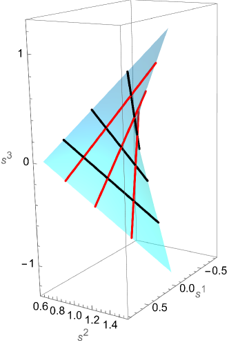
Figure 1: Using (38), we plot one octant of the Liouville soliton surface $\Sigma$. This surface is a hyperboloid of one sheet for the solitary wave solution (19) with $k=1,\omega=1,\alpha=1/4$. The centroaffine invariant is ${\cal I}=1/4^{6}$. The red curves are found using $v=-1/2,0,1/2$, while the black curves correspond to $u=-1/2,0,1/2$. All of these curves are lines, since the one-sheet hyperbolioid is a doubly ruled surface.

One can generalize these type of surfaces by choosing any particular functions of interest, such as general power-functions that depend on some parameter $p$. One example, given by $\Phi(u)=2\sqrt{\alpha}~{}ku^{p}$ and $\Psi(v)=-2\sqrt{\alpha}~{}\omega v^{p}$ leads to the parametric soliton solution

$$\lambda(u,v;p)=2p^{2}\,k\omega\,(uv)^{p-1}~{}\mathrm{sech}^{2}\left(\sqrt{\alpha}\xi^{p}\right)~{},$$ (42)

where $\xi^{p}=ku^{p}-\omega v^{p}$. The soliton solutions corresponding to $p=1,2,3$ are presented in Figs. 2 and 3.

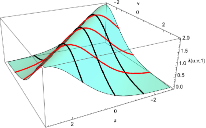
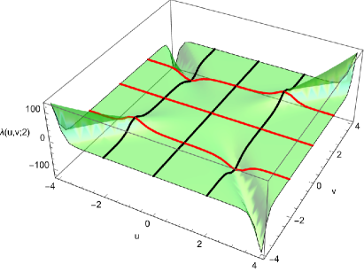
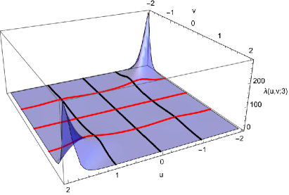
Figure 2: The parametric solution from (42) with $k=1,~{}\omega=1,~{}\alpha=1/4$, for $p=1,2,3$. The traces of each surface $u=-1/2,0,1/2$ (black color), and $v=-1/2,0,1/2$ (red color) are also displayed. These traces are the solitary waves corresponding to $p=1$, $p=2$, and $p=3$ from Fig. 3.

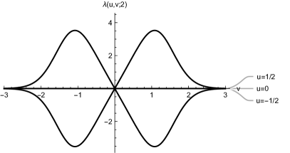
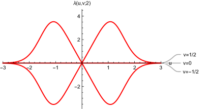
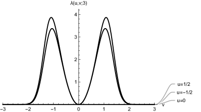
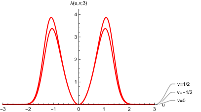
Figure 3: Solitary waves for $p=1$ (top), $p=2$ (middle), and $p=3$ (bottom), corresponding to the red and black curves of Fig. 2. The parameter $p$ acts a nonlinear power of the traveling wave variable, but more importantly as a parity operator of the amplitude of these pulses. If $p$ is odd and solitons are even we have only bright solitons, while if $p$ is even we have odd solitons which are bright and dark.

IV The modified variation of parameters method

Next, we present an equivalent method to obtain (19) based on a traveling wave ansatz, and by using a modified variation of parameters method which was first introduced by Kec̆kić in 1976 Keckic .

Effecting the logarithmic derivative, (1) becomes

$$\lambda\lambda_{uv}-\lambda_{u}\lambda_{v}=\alpha{\lambda}^{3}~{},$$ (43)

which can be turned into the ordinary differential equation

$${\lambda_{\xi}}^{2}-\lambda\lambda_{\xi\xi}=\frac{\alpha}{k\omega}{\lambda}^{3}~{},$$ (44)

using the traveling wave variable $\xi=ku-\omega v$. This equation can be written as a system of first order equations

$$\begin{array}[]{l}\lambda_{\xi}=\eta\equiv M(\lambda,\eta)~{},\\ \eta_{\xi}=\frac{1}{\lambda}\left({\eta}^{2}-\frac{\alpha}{k\omega}{\lambda}^{3}\right)\equiv N(\lambda,\eta)~{}.\end{array}$$ (45)

The system (45) is integrable since there is a first integral ${\cal H}(\lambda,\eta)\equiv const$ of (44) such that

$$\begin{array}[]{l}M(\lambda,\eta)=\mu(\lambda,\eta)\frac{\partial{\cal H}}{\partial\eta}~{},\\ N(\lambda,\eta)=-\mu(\lambda,\eta)\frac{\partial{\cal H}}{\partial\lambda}~{}.\end{array}$$ (46)

For the special case of unitary integrating factor $\mu(\lambda,\eta)\equiv 1$, then (45) is also Hamiltonian with first integral given by

$${\cal H}(\lambda,\eta)=\left(\frac{\eta}{\lambda}\right)^{2}+\frac{2\alpha}{k\omega}\lambda\equiv const~{},$$ (47)

and Hamiltonian curves shown in Fig. 4. These curves are very important in the phase space ($\lambda,\lambda_{\xi}$) because they depict the first integrals given by the constant energy ${\cal H}=const$.

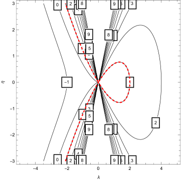
Figure 4: Hamiltonian curves for $k=1,~{}\omega=1,$ and $\alpha=1/4$. The dotted red curve corresponds to ${\cal H}=1$ and solution (59).

However, our system (46) holds true when the integrating factor is $\mu(\lambda,\eta)=\lambda^{2}/2$ for which (44) yields to the degenerate elliptic equation

$${\lambda_{\xi}}^{2}={\cal H}{\lambda}^{2}-\frac{2\alpha}{k\omega}{\lambda}^{3}~{}.$$ (48)

When $a\rightarrow\infty$ then $\alpha\rightarrow 0$, and the associated equation of (44) becomes

$${\lambda_{\xi}}^{2}-\lambda\lambda_{\xi\xi}=0~{}.$$ (49)

By one quadrature we obtain

$$\lambda_{\xi}=K\lambda~{},$$ (50)

while the second quadrature yields to the exponential solution

$$\lambda(\xi)=K_{0}e^{K\xi}~{},$$ (51)

with $K$ and $K_{0}$ arbitrary constants.

If we now suppose that $K$ is not a constant, i.e., $K=K(\lambda)$, by substituting (51) into (44) we obtain

$${\lambda_{\xi}}^{2}-\lambda\lambda_{\xi\xi}=-KK_{\lambda}{\lambda}^{3}~{},$$ (52)

which can be matched with (44) if $K(\lambda)$ is such that,

$$-KK_{\lambda}=\frac{\alpha}{k\omega}~{}.$$ (53)

The latter equation leads to

$$K(\lambda)=\sqrt{a_{2}-\frac{2\alpha}{k\omega}\lambda}~{},$$ (54)

where $a_{2}$ is an arbitrary constant. Letting $a_{3}=-\frac{2\alpha}{k\omega}$ then (54) becomes

$$\lambda_{\xi}=\lambda\sqrt{a_{2}+a_{3}\lambda}~{},$$ (55)

which is exactly (48) for $a_{2}={\cal H}$. This equation belongs to the general class of elliptic equations of the form (see also section 4 in gpr14 )

$${\lambda_{\xi}}^{2}=\sum_{i=0}^{3}a_{i}\lambda(\xi)^{i}\equiv Q_{3}(\lambda)~{},$$ (56)

which admit in general both cnoidal and solitary waves solutions. In our case, since $a_{0}=a_{1}=0$, then $\lambda=0$ is a double root of $Q_{3}(\lambda)$, and (56) admits only the solitary wave solutions

$$\lambda(\xi)=-\frac{a_{2}}{a_{3}}\mathrm{sech}^{2}\left[\frac{1}{2}\sqrt{a_{2}}(\xi-\xi_{0})\right],\quad a_{2}>0~{},$$ (57)

with $\xi_{0}$ an arbitrary constant. For $a_{2}=4\alpha$, and by taking $\xi_{0}=0$ with $a_{3}=-\frac{2\alpha}{k\omega}$, this solution corresponds to (19) with integral of motion given by ${\cal H}=1$, and

$${\lambda_{\xi}}^{2}={\lambda}^{2}-\frac{{\lambda}^{3}}{2}~{}.$$ (58)

In particular, for $\xi_{0}=0$, we obtain the soliton

$$\lambda(\xi)=2k\omega~{}\mathrm{sech}^{2}\left(\frac{\xi}{2}\right)~{}.$$ (59)

To end up this section, we notice that according to the above discussion the centroaffine invariant can be written directly in terms of the Hamiltonian constant of the soliton solution as

$${\cal I}=\left(\frac{{\cal H}}{k^{2}}\right)^{3}~{},$$ (60)

since for such solutions the Hamiltonian is a disguised form of the parameter entering the Liouville equation (2).

V A one-parameter Lax Pair

The second parametric third order matrix Lax pair for (2), known by Mikhailov Mikh , is given by

$$M=\begin{pmatrix}L_{11}\Lambda_{u}&0&L_{13}~{}e^{\Lambda/2}\\ 0&L_{22}\Lambda_{u}&0\\ 0&L_{32}e^{\Lambda/2}&0\end{pmatrix},\,\,\,\,\,\,\,N=\begin{pmatrix}A_{11}\Lambda_{v}&0&0\\ 0&A_{22}\Lambda_{v}&A_{23}~{}e^{\Lambda/2}\\ A_{31}~{}e^{\Lambda/2}&0&0\end{pmatrix}~{}.$$ (61)

These matrices also satisfy

$$\begin{array}[]{l}R_{u}=MR~{},\\ R_{v}=NR~{},\end{array}$$ (62)

for some general vector wave function $R^{T}(u,v)=\left(F(u,v),G(u,v),H(u,v)\right)$. This time, the compatibility condition leads to

$$\begin{pmatrix}A_{31}L_{13}\lambda-\frac{(A_{11}-L_{11})(\lambda_{u}\lambda_{v}-\lambda\lambda_{uv})}{\lambda^{2}}&0&\frac{(1-2A_{11})L_{13}\lambda_{v}}{2\sqrt{\lambda}}\\ 0&-A_{23}L_{32}\lambda+\frac{(A_{22}-L_{22})(\lambda_{u}\lambda_{v}-\lambda\lambda_{uv})}{\lambda^{2}}&\frac{A_{23}(L_{22}-1)}{2\sqrt{\lambda}}\lambda_{u}\\ \frac{-(1+2L_{11})A_{31}}{2\sqrt{\lambda}}\lambda_{u}&\frac{(1+2A_{22})L_{32}}{2\sqrt{\lambda}}\lambda_{v}&(A_{23}L_{23}-A_{31}L_{13})\lambda\end{pmatrix}\equiv 0~{}.$$ (63)

Identifying the terms in the matrix, we require

$$\begin{array}[]{ll}&A_{11}=\frac{1}{2}~{},\\ &L_{11}=-\frac{1}{2}~{},\\ &L_{22}=\frac{1}{2}~{},\\ &A_{22}=-\frac{1}{2}~{},\\ &A_{23}L_{32}=A_{31}L_{13}~{}.\end{array}$$ (69)

Choosing the parameters $L_{13}=\beta$ and $A_{31}=\frac{\alpha}{\beta}$, then $A_{23}=\beta$, and $B_{32}=\frac{\alpha}{\beta}$, and substituted into (61) leads to the one-parameter Lax pair

$$M=\begin{pmatrix}-\frac{\lambda_{u}}{2\lambda}&0&\beta\sqrt{\lambda}\\ 0&\frac{\lambda_{u}}{2\lambda}&0\\ 0&\frac{\alpha}{\beta}\sqrt{\lambda}&0\end{pmatrix},\,\,\,\,\,\,\,N=\begin{pmatrix}\frac{\lambda_{v}}{2\lambda}&0&0\\ 0&-\frac{\lambda_{v}}{2\lambda}&\beta\sqrt{\lambda}\\ \frac{\alpha}{\beta}\sqrt{\lambda}&0&0\end{pmatrix}~{}.$$ (70)

Now we will need to determine the eigenfunction $R(u,v)$ of the commutating differential operators which satisfy (62). The first equation of the system leads to

$$\begin{pmatrix}F_{u}+\frac{\lambda_{u}}{2\lambda}F-\beta\sqrt{\lambda}H\\ G_{u}-\frac{\lambda_{u}}{2\lambda}G\\ H_{u}-\frac{\alpha}{\beta}\sqrt{\lambda}G\end{pmatrix}=0~{},$$ (71)

while the second one gives

$$\begin{pmatrix}F_{v}-\frac{\lambda_{v}}{2\lambda}F\\ G_{v}+\frac{\lambda_{v}}{2\lambda}G-\beta\sqrt{\lambda}H\\ H_{v}-\frac{\alpha}{\beta}\sqrt{\lambda}F\end{pmatrix}=0~{}.$$ (72)

To solve these systems, we notice that we can integrate the second equation of the first set (71) to obtain

$$G(u,v)=c_{1}(v)\text{sech}\left(\sqrt{\alpha}\xi\right)~{}.$$ (73)

Using this result into the third equation and integrating again we can find

$$H(u,v)=\left[c_{1}(v)\frac{\sqrt{2\alpha\omega}}{\beta\sqrt{k}}\sinh\left(\sqrt{\alpha}\xi\right)+c_{2}(v)\cosh\left(\sqrt{\alpha}\xi\right)\right]\text{sech}\left(\sqrt{\alpha}\xi\right)~{}.$$ (74)

Since we have $H(u,v)$ up to the two integration constants, we integrate the first equation to obtain

$$F(u,v)=\left\{\frac{\left[c_{1}(v)\sqrt{\alpha}\omega\sinh\left(\sqrt{\alpha}\xi\right)+c_{2}(v)\sqrt{k\omega/2}\beta\cosh\left(\sqrt{\alpha}\xi\right)\right]^{2}}{\alpha k\omega c_{1}(v)}+c_{3}(v)\cosh^{2}\left(\sqrt{\alpha}\xi\right)\right\}\text{sech}\left(\sqrt{\alpha}\xi\right)~{}.$$ (75)

The arbitrary constants $c_{i}$ will be determined from the second system (72) by eliminating all the functions $F$, $H$ and their partial derivatives in $v$ to obtain only a third order equation on $G$, which after some cumbersome algebra reads

$$G_{vvv}-3\sqrt{\alpha}\omega\tanh\left(\sqrt{\alpha}\xi\right)G_{vv}-(\sqrt{\alpha}\omega)^{2}G_{v}+3(\sqrt{\alpha}\omega)^{3}\tanh\left(\sqrt{\alpha}\xi\right)G=0~{}.$$ (76)

Once we obtained this equation, we substitute $G(u,v)$ together with its partial derivatives, $G_{v}$, $G_{vv}$, and $G_{vvv}$ into (76), to hopefully obtain a manageable equation in $c_{1}$. Surprisingly, but not unexpected, the new ODE in $c_{1}$ is

$$c_{1}(v)^{\prime\prime\prime}-4\alpha\omega^{2}c_{1}(v)^{\prime}=0~{},$$ (77)

with the same equation as (22) but with $k$ replaced by $\omega$, and $u$ by $v$. Using

$$\begin{array}[]{ll}&c_{1}^{1}(v)=1~{},\\ &c_{1}^{2}(v)=\sinh(2\sqrt{\alpha}\omega v)~{},\\ &c_{1}^{3}(v)=\cosh(2\sqrt{\alpha}\omega v)~{},\end{array}$$ (81)

in (73), we obtain the solutions corresponding to $G(u,v)$ that are

$$\begin{array}[]{ll}&g^{1}(u,v)=\mathrm{sech}\left(\sqrt{\alpha}\xi\right)~{},\\ &g^{2}(u,v)=\sinh(2\sqrt{\alpha}\omega v)~{}\mathrm{sech}\left(\sqrt{\alpha}\xi\right)~{},\\ &g^{3}(u,v)=\cosh(2\sqrt{\alpha}\omega v)~{}\mathrm{sech}\left(\sqrt{\alpha}\xi\right)~{}.\\ \end{array}$$ (85)

The three solutions corresponding to $H(u,v)$ found from the second equation of (72) are

$$\begin{array}[]{ll}&h^{1}(u,v)=\sinh\left(\sqrt{\alpha}\xi\right)\mathrm{sech}\left(\sqrt{\alpha}\xi\right)~{},\\ &h^{2}(u,v)=\cosh\left(\sqrt{\alpha}\zeta\right)~{}\mathrm{sech}\left(\sqrt{\alpha}\xi\right)~{},\\ &h^{3}(u,v)=\mathrm{sinh}\left(\sqrt{\alpha}\zeta\right)~{}\mathrm{sech}\left(\sqrt{\alpha}\xi\right)~{}.\\ \end{array}$$ (89)

Finally, since we have $H$, we can use the third equation of system (72) to find the three corresponding $F(u,v)$, which are

$$\begin{array}[]{ll}&f^{1}(u,v)=\mathrm{sech}\left(\sqrt{\alpha}\xi\right)~{},\\ &f^{2}(u,v)=\sinh(2\sqrt{\alpha}ku)~{}\mathrm{sech}\left(\sqrt{\alpha}\xi\right)~{},\\ &f^{3}(u,v)=\cosh(2\sqrt{\alpha}ku)~{}\mathrm{sech}\left(\sqrt{\alpha}\xi\right)~{}.\\ \end{array}$$ (93)

Notice that these three functions satisfy the first equation of system (72), as they should. Combining all these functions (85) - (93), we can finally construct the two Darboux-transformed Liouville surfaces $\Sigma_{2}(f^{2},g^{2},h^{2})$, and $\Sigma_{3}(f^{3},g^{3},h^{3})$, which are presented in Fig. 5.

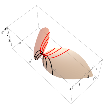
Figure 5: The Liouville soliton surfaces $\Sigma_{2}$ and $\Sigma_{3}$ corresponding to the Darboux-transformed Liouville solutions (32) for the same values $k=1,\omega=1,\alpha=1/4$. These are hyperbolic transformed surfaces corresponding to systems (85)-(93). The traces $u=-1/2,0,1/2$ (black color), and $v=-1/2,0,1/2$ (red color) have now kink-like shapes.

VI Summary and future prospects

In this paper, we have shown explicitly how soliton surfaces can be constructed based on the soliton solution of the Liouville equation in the travelling variable and its Darboux partner solutions. Similar surfaces can be constructed for other equations in the same class, such as the Tzitzéica equation (also known as Dodd-Bullough-Tzitéica equation), the Dodd-Bullough-Mikhailov (DBM) equation, and the Tzitzéica-Dodd-Bullough-Mikhailov(TDBM) equation, which written as (44), but with the coupling constant(s) in the power terms set to unity, have the form

$$\begin{array}[]{ll}&{\lambda_{\xi}}^{2}-\lambda\lambda_{\xi\xi}=-\frac{1-{\lambda}^{3}}{k^{2}-\omega^{2}}~{},\\ &{\lambda_{\xi}}^{2}-\lambda\lambda_{\xi\xi}=-\frac{1+{\lambda}^{3}}{k\omega}~{},\\ &{\lambda_{\xi}}^{2}-\lambda\lambda_{\xi\xi}=-\frac{(1+\lambda){\lambda}^{3}}{k\omega}~{},\\ \end{array}$$ (97)

respectively. This set of equations have similar ${\rm sech}^{2}$ soliton solutions zna , but the more complicated nonlinearities can generate cnoidal solutions. Consequently, periodic ‘cnoidal’ surfaces can be constructed. In fact, for any cubic or quartic polynomial in the right hand side of nonlinear equations of this type one can construct surfaces associated to their solutions following the method described here for the monomic Liouville case. We plan to study these surfaces in a future publication.

Acknowledgment

The authors wish to thanks the reviewers for useful comments and suggestions.

ORCID iDs

S.C. Mancas http://orcid.org/0000-0003-1175-6869
K.R. Acharya http://orcid.org/0000-0003-3551-7141
H.C. Rosu http://orcid.org/0000-0001-5909-1945

References

• (1) Sym A 1983 Soliton surfaces II Lett. Nuovo Cimento 36 307
• (2) Sym A 1985 Soliton surfaces and their applications Lecture Notes in Physics 239 editor Martini R (Berlin: Springer) 154
• (3) Cieśliński J 1998 The Darboux-Bianchi-Bäcklund transformation and soliton surfaces Proceedings of The First Non-Orthodox School on Nonlinearity and Geometry editors Wojcik D and Cieśliński J (Warszawa: Polish Scientific Publishers PWN) arXiv:1303.5472
• (4) Grundland A M, Post S 2012 Soliton surfaces via a zero-curvature representation of differential equations J. Phys. A: Math. Theor. 45 115204
• (5) Grundland A M, Post S, Riglioni D 2014 Soliton surfaces and generalized symmetries of integrable systems J. Phys. A: Math. Theor. 47 015201
• (6) Perelomov A M 1987 Chiral models: Geometrical aspects Phys. Rep. 146 135
• (7) Dai B, Terng C-L 2007 Bäcklund transformations, Ward solitons, and unitons J. Diff. Geom. 75 57
• (8) Mikhaĭlov A V 1979 Integrability of a two-dimensional generalization of the Toda chain JETP Lett. 30 414
• (9) Monge G 1850 Application de l’Analyse à la Géométrie 5th Edition (Paris: Bachelier) 597
• (10) Liouville J 1853 Sur l’équation aux différences partielles $d^{2}\,log\lambda/dudv\pm\lambda/2a^{2}=0$ J Math. Pures Appl. 18 71
• (11) Barbashov B M, Nesterenko V V 1980 Differential geometry and nonlinear field models Fortschritte der Physik 28 427
• (12) Teschner J 2001, Liouville theory revisited Class. Quant. Grav. 18, R153
• (13) Dzordzhadze G P, Pogrebkov A K, Polivanov M K 1979 Singular solutions of the equations $\square\phi+(m^{2}/2)\exp\phi=0$ and dynamics of singularities Theor. Math. Phys. 40 221
• (14) Johansson L, Kihlberg A, Marnelius R 1984 Sectors of solutions and minimal energies in classical Liouville theories for strings Phys. Rev. D 29, 2798
• (15) Tzitzéica G 1924 Géométrie Différentielle Projective des Réseaux (Bucharest: Cultura Naţională)
• (16) Tzitzéica G 1910 Sur une nouvelle classe de surfaces Comptes Rendus Acad. Sci. Paris 150 No. 16 955
• (17) Tzitzéica G 1910 Sur une nouvelle classe de surfaces Comptes Rendus Acad. Sci. Paris 150 No. 20 1227
• (18) Brezhnev Yu V 1996 Darboux transformation and some multi-phase solutions of the Dodd-Bullough-Tzitzéica equation: $U_{xt}=e^{U}-e^{-2U}$ Phys. Lett. A 211 94
• (19) Schief W K, Rogers C 1994 The affinsphären equation. Moutard and Bäcklund transformations Inverse Problems 10 711
• (20) Kec̆kić J D 1976 Addition to Kamke’s Treatise, VII: Variation of parameters for nonlinear second order differential equations Univ Beograd. Publ Elektrotehn FAK Ser. Mat. Fis. No. 544 - No. 576 31
• (21) Mancas S C, Rosu H C, Pérez-Maldonado M 2018 Traveling-wave solutions for wave equations with two exponential nonlinearities Zeitschrift für Naturforschung A 73 883