Study of Decoupled Gravastars in Energy-momentum Squared Gravity

Abstract

In this paper, we generate an exact anisotropic gravastar model using gravitational decoupling technique through minimal geometric deformation in the framework of $f(\Re,{T}^{2})$ gravity. This novel model explains an ultra-compact stellar configuration whose internal region is smoothly matched to the exterior region. The developed stellar model satisfies some of the essential characteristics of a physically acceptable model such as a positive monotonically decreasing profile of energy density from the center to the boundary and monotonically decreasing behavior of the pressure. The anisotropic factor and Schwarzschild spacetime follows physically acceptable behavior. We find that all the energy bounds are satisfied except strong energy condition inside the ultra-compact stellar structure for the coupling constant of this theory, which is compatible with the regularity condition.

Keywords: Modified theories; Decoupling; Gravastars; Israel formalism.
PACS: 04.50.Kd; 04.40.-b; 97.10.Cv.

1 Introduction

The current accelerated expansion of the cosmos has been the most significant development in recent years. This expansion is thought to be the result of a mysterious force having repulsive nature and is described as dark energy (DE). Several researchers have put forward their efforts to reveal its unknown features. The first proposal explaining the hidden characteristics of DE is the cosmological constant, but it suffers issues like fine-tuning and coincidence. Different modified versions have been presented to overcome these problems that are assumed to be fascinating approaches in revealing mysteries of the universe. The first modification is $f(\Re)$ theory of gravity which has a significant literature [1] to understand its physical properties. This modified theory was further generalized by incorporating the idea of curvature-matter coupling. Such coupling theories are non-conserved with an additional force that alters the path of the particle. The minimal coupling is introduced as $f(\Re,T)$ theory [2] whereas the non-minimally coupled theory is $f(\Re,T,\Re_{\sigma\gamma}T^{\sigma\gamma})$ gravity [3].

Different cosmic studies have been presented to understand the beginning of the universe. One of the extensively accepted proposals termed as big-bang theory is a remarkable framework describing evolutionary processes. According to this idea, all the matter in the cosmos expanded from a single point, referred to as a singularity. This theory portrays the beginning of the universe but this proposal suffers flatness problem, horizon problem and monopole problem. The research community is always curious and dedicates its effort to find answers to cosmological issues. The fascinating notion of bounce theory (based on repeated cosmic expanding and contracting behavior) serves as a backbone for introducing a new theory. This newly introduced concept resolves big bang issues by resolving singularity and provides a better explanation of accelerated expanding cosmic behavior.

Katrici and Kavuk [4] constructed an extension of $f(\Re)$ theory that incorporates the concept of bounce theory. They developed a particular coupling between matter and gravity through self-contraction of the energy-momentum tensor (EMT) referred to as energy-momentum squared gravity (EMSG) or known as $f(\Re,{T}^{2})$ theory, where $T^{2}=T_{\sigma\gamma}T^{\sigma\gamma}$. This proposal with a minimum scale factor as well as finite maximum energy density is considered to be a suitable framework to overcome big-bang problem. The cosmological constant resolves the big-bang singularity by providing the repulsive force in the background of this theory. This theory follows the true sequence of cosmological eras and effectively describes cosmic behavior. The field equations involve squared and product components of matter variables, which are useful in studying different cosmological scenarios.

Roshan and Shojai [5] computed the exact solution by solving EMSG field equations with homogeneous isotropic spacetime and demonstrated the possibility of a bounce in the early universe. Board and Barrow [6] calculated the range of exact solutions for an isotropic expanding universe in reference to early and late-time evolution. Nari and Roshan [7] determined a connection between mass and the radius of neutron stars. They found that a smaller or larger value of mass is governed by the central pressure of these stars and the value of model parameter of this gravity. Bahamonde et al. [8] used different coupling models to study the expansion of the universe and concluded that these models help in understanding the present accelerated cosmic expansion. We have studied various attributes of charged as well as uncharged gravastar solutions [9]. Recently, Sharif and his collaborators studied decoupled solutions [10] as well as the impact of charge on complexity of static sphere in the same theory [11].

Different cosmic phenomena, such as the origin and evolution of celestial bodies have captivated the interest of various researchers. Among all the cosmic objects, stars are the core components of galaxies, which are organized systematically in a cosmic web. When a star runs out of fuel, its outward pressure vanishes, leading to gravitational collapse and hence compact objects are formed. A black hole is such a stellar remnant which is a totally collapsed entity with a singularity hidden behind an event horizon. Mazur and Motolla [12] developed a compact model (gravastar) as an alternative to black hole to avoid singularity and event horizon. Motolla [13] discussed in detail dark energy and condensate stars. The resulting gravitational condensate star configuration resolves all black hole paradoxes, and provides a testable alternative to black holes as the final state of complete gravitational collapse. Mazur and Motolla [14] studied pressure and negative pressure interior of a non-singular black hole. In contrast to black holes, the significant feature of this hypothetical object is its singularity-free nature. Three regions constitute the complete gravastar structure, internal and external regions separated by a thin shell. The DE in the inner domain causes a repulsive force which contributes as a main barrier to overcome singularity formation. The intermediate shell surrounding the inner boundary exerts an inward force and thus hydrostatic equilibrium is maintained while the Schwarzschild metric characterizes the exterior region. Moreover, each region is described by a specific equation of state (EoS).

Visser and Wiltshire [15] examined the stability of gravastars towards radial perturbations and concluded that a viable EoS results in the stability of gravastar in GR. This work was extended by examining appropriate constraints for the stability of gravastar solutions [16]. Cattoen et al. [17] studied the usual gravastar structures and concluded that the cosmic configuration has anisotropy in the absence of intermediate shell. Bilic et al. [18] formulated gravastar solutions by replacing the inner Born-Infeld phantom metric with the de Sitter geometry which represent compact objects at the galactic center. Horvat and Ilijic [19] discussed the stability of gravastars by employing the speed of sound criteria on thin-shell to determine compactness bounds. Ovalle [20] discussed anisotropic gravastars by means of decoupling approach.

Many researchers have also investigated the formation as well as fundamental physical characteristics of gravastars in modified theories of gravity. Das et al. [21] discussed isotropic gravastar structure in the realm of ${f(\Re,T)}$ gravity. They obtained a linear profile of physical features in relation to shell thickness. Shamir and Ahmad [22] constructed spherically symmetric gravastar models whose characteristics obey an increasing trend with respect to the thickness. Different physical features of charged/uncharged gravastar model were studied in $f(\mathbb{T})$ theory ($f(\mathbb{T})$ is an arbitrary function of the torsion scalar) [23]. Abbas and Majeed [24] discussed isotropic gravastar structure in the background of Rastall gravity. Yousaf et al. [25] examined the gravastar model in modified theory and found that length, energy and entropy present an increasing trend with respect to thickness. In the background of ${f(\Re,\mathcal{G})}$ gravity ($\mathcal{G}$ defines the Gauss-Bonnet invariant), Bhatti et al. [26] investigated different physical characteristics related to intrinsic shell thickness and found accepted behavior. Ray et al. [27] provided a very good review on the entire aspects of gravastar as envisioned by Mazur and Mottola starting from the black hole physics to its present state and enlightening the future works. The gravastar models in a number of modified gravity models starting from $f(R,T)$ to Rastall-Rainbow gravity have been reviewed. Bhatti and his collaborators [28] discussed charged/uncharged gravastar model in ${f(\mathcal{G})}$ gravity to analyze different features. Bhar and Rej [29] studied the role of electromagnetic field in the stability of gravastar structure.

Cosmological solutions are very important to comprehend the structural properties as well as the mechanism of celestial structures. However, it is usually difficult to obtain exact solutions due to the presence of highly non-linear terms in the field equations. In this regard, the gravitational decoupling technique by minimal geometric deformation (MGD) has recently been developed to determine the astrophysical and cosmic solutions. Ovalle [30] firstly introduced this concept from the viewpoint of braneworld. This approach connects a new gravitational source to the EMT of the seed matter distribution through a non-dimensional parameter. In this scheme, the deformation is employed only on the radial metric function while leaving the temporal metric component unaltered. Consequently, two sets of nonlinear field equations are formed, one for the new source and the other for the seed source. The decoupling method has extensively been used to transform isotropic spherical solutions into anisotropic ones.

The isotropic, anisotropic, and charged fluid configurations are the key topics for researchers in the context of compact celestial bodies. Ovalle et al. [31] extended isotropic solutions by assuming Tolman IV spacetime in the inner region. Ovalle and his collaborators [32] investigated ultra-compact stars through decoupling technique without altering any of the fundamental property. Gabbanelli et al. [33] computed acceptable anisotropic solutions by considering the Durgapal-Fuloria stellar configuration in the interior region. Graterol [34] implemented this technique to determine anisotropic solutions by considering Buchdahl isotropic solution. The extensions of isotropic solutions were obtained by using Krori-Barua (KB) spacetime [35]. Morales and Tello-Ortiz [36] studied charged Heintzmann anisotropic solution and graphically examined matter variables for various stars. Maurya et al. [37] explored the influence of anisotropy by taking Korkina-Orlyanskii isotropic matter distribution.

Many viable and stable solutions have been studied by using the decoupling technique in modified theories. Sharif and Majid [38] obtained anisotropic solutions by using different well-known isotropic solutions in Brans-Dicke theory. Maurya et al. [39] explored anisotropic solutions by assuming Korkina-Orlyanskii spacetime in the inner domain in $f(\Re,T)$ theory. Zubair and Azmat [40] extended Tolman VII solution in the same theory. Sharif and Naseer [41] evaluated charged/uncharged anisotropic extensions of KB metric in non-minimal curvature-matter coupled theory. Recently, Azmat et al. [42] employed this technique to investigate physical features of anisotropic gravastar in $f(\Re,T)$ theory. The departure from the isotropic scenario leads to an interesting situation, giving rise to an intriguing phenomenon inside the stellar interior, i.e., the system experiences a repulsive force that counteracts the gravitational gradient, which allows the construction of more compact and massive objects. This inspired us to develop anisotropic gravastars in the background of $f(\Re,T^{2})$ providing interesting results.

The aim of this article is to study the anisotropic gravastar in the background of $f(\Re,{T}^{2})$ theory. We use gravitational decoupling through MGD scheme to include the impact of anisotropy in the fluid configuration of the gravastar. The paper is organized as follows. Section 2 demonstrates the complete array of the field equations corresponding to both sources (seed and source). The solutions are decoupled in section 3 which are smoothly joined at the stellar surface. Section 4 describes MGD gravastar configuration which meets some of the viable characteristics of a stellar structure. We summarize our results in the last section.

2 Basic Formalism

The action of this theory involving matter Lagrangian density ($\L_{m}$) and the Lagrangian density ($\L_{\tau}$) of an additional source ($\tau$) is characterized by

$$S=\int d^{4}x\left(\frac{1}{2k^{2}}f(\Re,T^{2})+{\L}_{m}+\aleph{\L}_{\tau}\right)\sqrt{-g}.$$ (1)

The coupling constant is $k^{2}=8\pi$, determinant of the metric tensor is denoted by $g$ and $\aleph$ symbolizes the decoupling parameter. The action (1) provides the following field equations

$$\Re_{\sigma\gamma}f_{\Re}+g_{\sigma\gamma}\Box f_{\Re}-\nabla_{\sigma}\nabla_{\gamma}f_{\Re}-\frac{1}{2}g_{\sigma\gamma}f=8\pi\left(T_{\sigma\gamma}+\aleph\tau_{\sigma\gamma}\right)-f_{T^{2}}\circleddash_{\sigma\gamma},$$ (2)

here $f_{\Re}=\frac{\partial{f}}{\partial{\Re}}$ and $f_{T^{2}}=\frac{\partial{f}}{\partial{T^{2}}}$. The self contraction of del operator defines d’Alembert operator ($\Box=\nabla_{\sigma}\nabla^{\sigma}$), whereas the tensor $\circleddash_{\sigma\gamma}$ is

$$\circleddash_{\sigma\gamma}=-2{\L}_{m}(T_{\sigma\gamma}-\frac{1}{2}g_{\sigma\gamma}T)-4\frac{\partial^{2}{{\L}_{m}}}{\partial{g^{\sigma\gamma}}{\partial{g^{\alpha\delta}}}}T^{\alpha\delta}-TT_{\sigma\gamma}+2T^{\delta}_{\sigma}T_{\gamma\delta}.$$ (3)

The EMT of seed and additional sources are, respectively

$$T_{\sigma\gamma}=g_{\sigma\gamma}{\L}_{m}-2\frac{\partial{\L}_{m}}{\partial g^{\sigma\gamma}},\quad\tau_{\sigma\gamma}=g_{\sigma\gamma}{\L}_{\tau}-2\frac{\partial{\L}_{\tau}}{\partial g^{\sigma\gamma}}.$$ (4)

The isotropic matter configuration involving density, pressure and four-velocity corresponds to the seed source given as follows

$$T_{\sigma\gamma}=(\varrho+P)U_{\sigma}U_{\gamma}-g_{\sigma\gamma}P,$$ (5)

with $U_{\gamma}U^{\gamma}=1$. Moreover, plugging $L_{m}=-P$ in Eq.(3) yields

$$\circleddash_{\sigma\gamma}=(3P^{2}+\varrho^{2}+4P\varrho)U_{\sigma}U_{\gamma}.$$ (6)

Rearrangement of Eq.(2) gives

$$G_{\sigma\gamma}=\frac{1}{f_{\Re}}\Bigg{(}8\pi(T_{\sigma\gamma}+\aleph\tau_{\sigma\gamma})-g_{\sigma\gamma}\Box f_{\Re}+\nabla_{\sigma}\nabla_{\gamma}f_{\Re}-\circleddash_{\sigma\gamma}f_{T^{2}}+\frac{1}{2}g_{\sigma\gamma}(f-\Re f_{\Re})\Bigg{)},$$ (7)

where $G_{\sigma\gamma}=\Re_{\sigma\gamma}-\frac{1}{2}\Re g_{\sigma\gamma}$ is the Einstein tensor.

The static spherical object is described by the following line element

$$ds^{2}=e^{\varphi}dt^{2}-e^{\psi}dr^{2}-r^{2}d\theta^{2}-r^{2}\sin^{2}\theta d\phi^{2},$$ (8)

where the metric coefficients $\varphi$ and $\psi$ are functions of radial coordinate only. The complexity of the field equations is reduced by considering minimally coupled model $f(\Re,T^{2})=\Re+\zeta T^{2}$ ($\zeta$ is the coupling parameter) and the respective equations take the following form

$$8\pi(\widetilde{\varrho}+\aleph\tau^{t}_{t}) = e^{-\psi}(\frac{\psi^{{}^{\prime}}}{r}-\frac{1}{r^{2}})+\frac{1}{r^{2}},$$ (9)

$$8\pi(\widetilde{P}-\aleph\tau^{r}_{r}) = e^{-\psi}(\frac{\varphi^{{}^{\prime}}}{r}+\frac{1}{r^{2}})-\frac{1}{r^{2}},$$ (10)

$$8\pi(\widetilde{P}-\aleph\tau^{\theta}_{\theta}) = \frac{e^{-\psi}}{4}(2\varphi^{{}^{\prime\prime}}-\frac{2\psi^{{}^{\prime}}}{r}+\frac{2\varphi^{{}^{\prime}}}{r}-\varphi^{{}^{\prime}}\psi^{{}^{\prime}}+\varphi^{{}^{\prime}2}).$$ (11)

Here prime exhibits radial derivative whereas ($\widetilde{\varrho}$, $\widetilde{P}$) are provided by

$$\widetilde{\varrho} = \varrho-\frac{1}{16\pi}(3P^{2}+8\varrho P+\varrho^{2})\zeta,$$ (12)

$$\widetilde{P} = P-\frac{1}{16\pi}(3P^{2}+\varrho^{2})\zeta.$$ (13)

The conservation law is violated in this theory and hence covariant differentiation of Eq.(7) gives

$$\nabla^{\sigma}(\Theta_{\sigma\gamma}f_{T^{2}})-\frac{1}{2}g_{\sigma\gamma}\nabla^{\sigma}f=P^{{}^{\prime}}+\frac{\varphi^{{}^{\prime}}}{2}(\varrho+P)+\aleph\left(\frac{\varphi^{{}^{\prime}}}{2}(\tau^{t}_{t}-\tau^{r}_{r})\right.+\left.\frac{2}{r}(\tau^{\theta}_{\theta}-\tau^{r}_{r})-\tau^{r^{\prime}}_{r}\right).$$ (14)

The highly non-linear field equations involve seven unknown functions: state variables $(\widetilde{\rho},\widetilde{P})$, metric coefficients $(\varphi,\psi)$ and components of extra source $(\tau^{t}_{t},\tau^{r}_{r},\tau^{\theta}_{\theta})$. The total energy density, radial/tangential pressure are respectively, given as

$$\hat{\varrho}=\widetilde{\varrho}+\aleph\tau^{t}_{t},\quad\hat{P_{r}}=\widetilde{P}-\aleph\tau^{r}_{r},\quad\hat{P_{t}}=\widetilde{P}-\aleph\tau^{\theta}_{\theta}.$$ (15)

Moreover, the presence of an additional source with $\tau^{r}_{r}\neq\tau^{\theta}_{\theta}$ generates anisotropy in the inner domain of self-gravitating body having the form

$$\hat{\Delta}=\hat{P_{t}}-\hat{P_{r}}=\aleph(\tau^{r}_{r}-\tau^{\theta}_{\theta}).$$ (16)

If $\zeta\rightarrow 0$, the field equations in $f(\Re,T^{2})$ gravity will reduce to GR.

3 Minimal Geometric Decoupling Scheme

In this section, the solution of the field equations are discussed through MGD approach. To encode the influence of extra source in isotropic matter distribution, the metric potentials ($\xi$ and $\varpi$) are modified in the following manner

$$\xi\rightarrow\varphi=\xi+\aleph j(r),\quad\varpi\rightarrow e^{-\psi}=\varpi+\aleph\varsigma,$$ (17)

where $j(r)$ and $\varsigma(r)$ present temporal and radial deformations, respectively. Employing MGD scheme (alters only radial function through geometric deformation while keeping the temporal metric function unchanged, i.e., $j(r)=0$), we have two sets of the decoupled solutions. The first array is given by

$$8\pi\widetilde{\varrho} = \frac{1}{r^{2}}-(\frac{\varpi}{r^{2}}+\frac{\varpi^{{}^{\prime}}}{r})=8\pi\varrho-\frac{1}{2}(\varrho^{2}+3P^{2}+8\varrho P)\zeta,$$ (18)

$$8\pi\widetilde{P} = -\frac{1}{r^{2}}+\frac{\varpi}{r}(\frac{1}{r}+\varphi^{{}^{\prime}})=8\pi P-\frac{1}{2}(\varrho^{2}+3P^{2})\zeta,$$ (19)

$$8\pi\widetilde{P} = \frac{\varpi}{2}(\varphi^{{}^{\prime\prime}}+\frac{\varphi^{{}^{\prime}2}}{2}+\frac{\varphi^{{}^{\prime}}}{r})+\frac{\varpi^{{}^{\prime}}}{2}(\frac{\varphi^{{}^{\prime}}}{2}+\frac{1}{r})=8\pi P-\frac{1}{2}(\varrho^{2}+3P^{2})\zeta,$$ (20)

whereas, the second array including the impact of extra source is

$$8\pi\tau^{t}_{t} = -\frac{\varsigma^{{}^{\prime}}}{r}-\frac{\varsigma}{r^{2}},$$ (21)

$$8\pi\tau^{r}_{r} = -\frac{\varsigma}{r}(\frac{1}{r}+\varphi^{{}^{\prime}}),$$ (22)

$$8\pi\tau^{\theta}_{\theta} = -(\frac{\varphi^{{}^{\prime}}}{r}+\varphi^{{}^{\prime\prime}}+\frac{\varphi^{{}^{\prime}2}}{2})\frac{2\varsigma}{r}-\varsigma^{{}^{\prime}}(\frac{\varphi^{{}^{\prime}}}{4}+\frac{1}{2r}).$$ (23)

Equation (14) can be splitted into isotropic and anisotropic sectors as

$$\nabla^{\sigma}(\circleddash_{\sigma\gamma}f_{T^{2}})-\frac{1}{2}g_{\sigma\gamma}\nabla^{\sigma}f = (\widetilde{P})^{{}^{\prime}}+\frac{\varphi^{{}^{\prime}}}{2}(\widetilde{\varrho}+\widetilde{P}),$$ (24)

$$\tau^{r^{\prime}}_{r}-\frac{\varphi^{{}^{\prime}}}{2}(\tau^{t}_{t}-\tau^{r}_{r})-\frac{2}{r}(\tau^{\theta}_{\theta}-\tau^{r}_{r}) = 0.$$ (25)

We consider a standard barotropic EoS to simplify the field equations as

$$\varrho=\frac{m}{V},$$ (26)

where $m$ and $V=\frac{4}{3}\pi{r}^{3}$ describe the mass and volume of the sphere. Using this EoS, the matter variables (density and pressure) read as follows

$$\widetilde{\varrho} = \frac{3m\left(-9\zeta m+16\pi^{2}r^{3}\right)}{64\pi^{3}r^{6}},$$ (27)

$$\widetilde{P} = \frac{48\pi^{2}mr^{3}-9\zeta m^{2}}{64\pi^{3}r^{6}},$$ (28)

which contribute considerably in studying the influence of anisotropy.

3.1 Matching Condition

The deformed Schwarzschild spacetime describing the exterior region, is modified trough $\tau$-sector and is described as [32]

$$ds^{2}_{+}=\left(1-\frac{2\mathcal{M}}{r}\right)dt^{2}-\left(1-\frac{2\mathcal{M}}{r}+\mathcal{V}g^{\star}(r)\right)^{-1}dr^{2}-r^{2}d\theta^{2}-r^{2}\sin^{2}\theta d\phi^{2},$$ (29)

The decoupling function for the exterior Schwarzschild metric is $g^{\star}(r)$, which appears to the extra source ${\tau_{\sigma\gamma}^{+}}$. It is mentioned here that the internal $\varsigma$ and external $g^{\star}(r)$ deformations are not identical. Likewise, the respective parameters $\aleph$ and $\mathcal{V}$ are not identical and govern the deformations in their respective sectors. The anisotropic source ${\tau_{\sigma\gamma}^{+}}\neq 0$ may impact exterior geometry and it is no more vacuum. Moreover, when decoupling is employed to the Schwarzschild vacuum as well as additional external source, Eqs.(21)-(23) for the external geometry give

$$(\tau^{t}_{t})^{+} = -\frac{g^{\star}}{r^{2}}-\frac{(g^{\star})^{{}^{\prime}}}{r},$$ (30)

$$(\tau^{r}_{r})^{+} = -\frac{g^{\star}}{r(r-2\mathcal{M})},$$ (31)

$$(\tau^{\theta}_{\theta})^{+} = \frac{\mathcal{M}(r-\mathcal{M})}{r^{2}(r-2\mathcal{M})}g^{\star}-\frac{r-\mathcal{M}}{2r(r-2\mathcal{M})}(g^{\star})^{{}^{\prime}}.$$ (32)

Junctions conditions are essential for joining the inner and outer geometries at the hypersurface $(\Sigma:r=\mathfrak{R})$. Israel junction conditions have two fundamental forms. The first form reads the continuity of metric potentials

$$({ds^{2}})_{\Sigma}=0.$$ (33)

At stellar surface, we have

$$e^{\varphi}=1-\frac{2\mathcal{M}}{\mathfrak{R}},$$ (34)

and

$$1-\frac{2M}{\mathfrak{R}}+\aleph\varsigma(r)=1-\frac{2\mathcal{M}}{\mathfrak{R}}+\mathcal{V}g^{\star}(r).$$ (35)

while the second form is

$$(T^{1}_{1})^{-1}-\aleph(\tau^{r}_{r})^{-}=-\mathcal{V}(\tau^{r}_{r})^{+}.$$ (36)

This condition leads to the continuity of pressure in the radial direction at the hypersurface.

4 MGD Gravastars in EMSG

Following Mazur and Mottola gravastar model [12], we use the EoS, $\mathcal{W}\varrho=P$ with $\mathcal{W}$ describing the EoS parameter. The inner gravastar domain follows DE EoS $\varrho=-P$ (for $\mathcal{W}=-1$). The negative pressure in this region provides repulsive force. Employing DE EoS along with Eq.(14) yields $\varrho=\varrho_{0}$(constant) which gives

$$\varpi=1-\frac{2{\rho_{0}}{r^{2}}}{3}(4\pi+\zeta{\varrho_{0}})+\frac{C_{1}}{r},$$ (37)

In order to avoid singularity, we take the arbitrary constant $C_{1}$ to be zero at core. Thus we have

$$\varpi=1-\frac{2{\varrho_{0}}{r^{2}}}{3}(4\pi+\zeta{\varrho_{0}}).$$ (38)

The temporal and radial metric functions are connected as follows

$$e^{-\varphi}={C_{2}}\varpi,$$ (39)

The mass corresponding to the inner region is

$$M(\mathfrak{R})=\frac{{\varrho_{0}(4\pi+\zeta{\varrho_{0}})}\mathfrak{R}^{3}}{3}.$$ (40)

Applying the deformation metric potentials in explicit form, we have

$$e^{\varphi} = {C_{2}}(1-{\mathcal{P}}^{2}r^{2}),$$ (41)

$$\varpi = 1-{\mathcal{P}}^{2}r^{2},$$ (42)

where

$$\mathcal{P}^{2}=\frac{\varrho_{0}}{3}\left(8\pi+2\zeta\varrho_{0}\right)=\frac{2\mathcal{M}}{\mathfrak{R}^{3}}=\frac{\mathfrak{R}_{s}}{\mathfrak{R}^{3}}.$$ (43)

Here, $\mathcal{M}$ is the mass and $\mathfrak{R}$ denotes radius of the star. Moreover, $\mathfrak{R}_{s}$ is the Schwarzschild radius and $\varrho_{0}$ is the constant energy density.

The deformed gravastar solution is developed by using the MGD approach yielding

$$e^{\varphi} = {C_{2}}(1-{\mathcal{P}}^{2}r^{2}),$$ (44)

$$e^{-\psi} = 1-{\mathcal{P}}^{2}r^{2}+\aleph\varsigma(r).$$ (45)

We solve the system of equations (21)-(23) to obtain the deformation function. To determine the remaining components of extra source, the characteristic of gravastar ($g_{00}=g_{11}^{-1}=0$) at the stellar surface $r=\mathfrak{R}_{s}$ is assumed. To preserve this property in the deformed metric components of gravastar ((44) and (45)), the geometric deformation function satisfies

$$\varsigma(r)\sim 1-{\mathcal{P}}^{2}r^{2}.$$ (46)

The simplest choice is

$$\varsigma(r)\sim(1-{\mathcal{P}}^{2}r^{2}){\mathcal{P}}^{n}r^{n},~{}~{}~{}~{}n\geq 2.$$ (47)

This condition on $n$ is very significant to obtain non-singular solutions. The expression for the radial metric component (45) is evaluated as

$$e^{-\psi}=(1-{\mathcal{P}}^{2}r^{2})({1+\aleph\mathcal{P}}^{n}r^{n}).$$ (48)

We take a constraint, $\aleph\geq-1$, to have finite positive value at $r=\mathfrak{R}_{s}$. Consequently, we obtain matter variables as follows

$$\hat{\varrho} = \widetilde{\varrho}+\aleph\mathcal{P}^{n}r^{n-2}\left((n+3){\mathcal{P}}^{2}r^{2}-n-1\right),$$ (49)

$$\hat{P_{r}} = \widetilde{P}-\aleph{\mathcal{P}}^{n}{r}^{n-2}\left(3{\mathcal{P}}^{2}{r}^{2}-1\right),$$ (50)

$$\hat{P_{t}} = \widetilde{P}-\aleph{\mathcal{P}}^{n}{r}^{n-2}\Big{[}\left(n+3\right){\mathcal{P}}^{2}{r}^{2}-\frac{n}{2}\Big{]}.$$ (51)

It can be easily seen from Eqs.(49)-(51) that only $n\geq 2$ provides singularity-free solutions, whereas the anisotropic factor is given by

$$\hat{\Delta}=\hat{P_{t}}-\hat{P_{r}}=\frac{\aleph{\mathcal{P}}^{n}{r}^{n-2}}{2}\left(n-2-2n\mathcal{P}^{2}r^{2}\right).$$ (52)

The expressions (48)-(51) along with (44) represent an ultra-compact non-uniform anisotropic gravastar structure. Further, we consider gravastar solution obtained after employing deformation, given in Eqs.(44) and (48) along with Eqs.(34) and (35) providing continuity of metric potentials implying that

$$1-\frac{2\mathcal{M}}{\mathfrak{R}}=0,$$ (53)

$$1-\frac{2\mathcal{M}}{\mathfrak{R}}+\mathcal{V}g^{\star}_{\mathfrak{R}}=0.$$ (54)

The primary feature of the gravastar configuration ($g_{00}=g_{11}^{-1}=0$ at Schwarzschild radius) gives zero in the above equations. Equation (54) yields

$$g^{\star}_{\mathfrak{R}}\sim\frac{2\mathcal{M}-\mathfrak{R}}{\mathfrak{R}}=0$$ (55)

Equation (55) shows that the deformation disappears at the surface of gravastar geometry

$$\frac{48\pi^{2}Mr^{3}-27\zeta M^{2}}{64\pi^{3}r^{6}}-\frac{2\aleph}{r^{2}}=\frac{g^{\star}_{\mathfrak{R}}}{\mathfrak{R}-2\mathcal{M}}.$$ (56)

Equations (53), (55) and (56) give the necessary and sufficient constraints for smooth matching of internal (8) and external geometries (29). Furthermore, considering the standard Schwarzschild spacetime, we obtain the decoupling parameter

$$\aleph=\frac{3\left(16\pi^{2}Mr^{3}-9\zeta M^{2}\right)}{128\pi^{3}r^{4}}.$$ (57)

Figure 1 shows acceptable behavior of state variables for this value of $\aleph$. We see that density has positive decreasing profile while the pressure is negative. The inner gravastar geometry possesses negative pressure providing repulsive behavior. The anisotropic factor follows decreasing trend. To obtain the exterior deformed solution, we consider

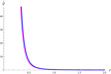
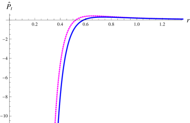
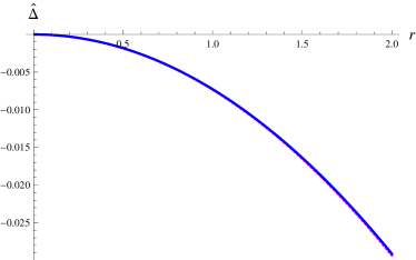
Figure 1: Plots of density, radial/tangential pressure and anisotropy for $\aleph=2.5$ (Magenta) and $\aleph=3.5$ (Blue) of the interior region.

$${\tau^{\sigma}_{\sigma}}^{+}=0.$$ (58)

Using Eqs.(30)-(32) in the above relation, we obtain

$$r(6\mathcal{M}^{2}+2r^{2}-7\mathcal{M}r){\varsigma}^{\prime}(r)+2(3\mathcal{M}^{2}+r^{2}-4\mathcal{M}r)\varsigma(r)=0,$$ (59)

whose solution yields

$$g^{\star}(r)=\frac{l_{c}\left(1-\frac{2M}{r}\right)}{2r-3M}.$$ (60)

Here, $l_{c}$ denotes constant having dimension of length. Thus, the deformed exterior solution is given as

$$e^{-\psi}=\left(1-\frac{2\mathcal{M}}{\mathfrak{R}}\right)\left(1+\frac{l}{2r-3\mathcal{M}}\right).$$ (61)

For $r>>\mathcal{M}$, it takes the form

$$e^{-\psi}\sim 1+\frac{l-4\mathcal{M}}{2r}.$$ (62)

The matter variables corresponding to the exterior region become

$$(\hat{\varrho})^{+}=(\tau^{t}_{t})^{+} = -\frac{l\mathcal{M}}{{\left(2r-3\mathcal{M}\right)^{2}}r^{2}},$$ (63)

$$(\hat{P_{r}})^{+}=(\tau^{r}_{r})^{+} = \frac{l}{{\left(2r-3\mathcal{M}\right)r^{2}}},$$ (64)

$$(\hat{P_{t}})^{+}=(\tau^{\theta}_{\theta})^{+} = -\frac{l\left(r-\mathcal{M}\right)}{{\left(2r-3\mathcal{M}\right)^{2}}r^{2}}.$$ (65)

The exterior metric anisotropy turns out to be

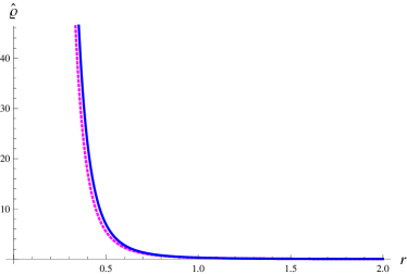
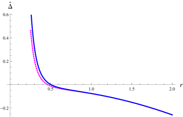
Figure 2: Behavior of density, radial/tangential pressure and anisotropy for $\aleph=2.5$ (Magenta) and $\aleph=3.5$ (Blue) of the exterior region.

$$(\hat{\Delta})^{+}=\frac{l(3r-4\mathcal{M})}{\left(2r-3\mathcal{M}\right)^{2}r^{2}}.$$ (66)

The deformed external metric will be regular for the following value of decoupling parameter

$$\aleph=\frac{-27\zeta M^{2}+48\pi^{2}Mr^{3}+64\pi^{3}r^{6}}{128\pi^{3}r^{6}},\quad\\ l=-\mathcal{M}$$ (67)

The restriction $n\geq 2$ is very significant as it allows smooth matching of the internal region with the external. The behavior of state variables corresponding to the above decoupling parameter and anisotropy is plotted in Figure 2. We find monotonically decreasing profile of density, negative pressure, and positive anisotropy.

The left and right plots in Figure 3 indicate Schwarzschild and deformed Schwarzschild metrics, respectively. The behavior of deformed Schwarzschild spacetime is physically acceptable but is totally different from that of standard Schwarzschild (linear profile). Figure 4 provides positive finite behavior of the metric functions of the inner and outer regions and cusp like trend is observed at joining point. This shows non-analytic behavior which implies violation of the second junction condition. From the general formalism of the Israel junction conditions, a violation of the second junction condition implies the presence of a $\delta$-distribution of stresses located on the hypersurface $\mathfrak{R}_{s}$. Finally, we investigate some physical characteristics of anisotropic solutions. The existence of ordinary matter as well as viability of the obtained solutions can be ensured by applying energy bounds which are classified into weak, dominant, null as well as strong energy conditions. For anisotropic matter distribution, these energy bounds are described by

Figure 3: Plots of the standard Schwarzschild (left) and deformed Schwarzschild (right) exterior.

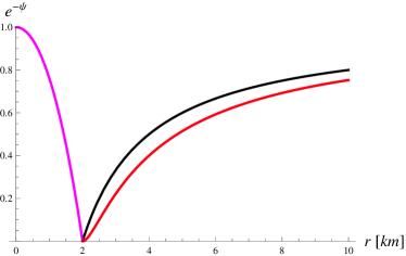
Figure 4: Graphical trend of the metric functions - interior function (Magenta), standard Schwarzschild (Black) and deformed Schwarzschild (Red).

$$\text{WEC:}\quad\hat{\varrho}\geq 0,\quad\hat{\varrho}+\hat{P_{r}}\geq 0,\quad\hat{\varrho}+\hat{P_{t}}\geq 0,$$

$$\text{DEC:}\quad\hat{\varrho}-|\hat{P_{r}}|\geq 0,\quad\hat{\varrho}-|\hat{P_{t}}|\geq 0,$$

$$\text{NEC:}\quad\hat{\varrho}+\hat{P_{r}}\geq 0,\quad\hat{\varrho}+\hat{P_{t}}\geq 0,$$

$$\text{SEC:}\quad\hat{\varrho}+\hat{P_{r}}\geq 0,\quad\hat{\varrho}+\hat{P_{t}}\geq 0,\quad\hat{\varrho}+\hat{P_{r}}+2\hat{P_{t}}\geq 0.$$

Figures 5 and 6 represent that all energy bounds except SEC are satisfied and thus the resulting solution follows physical viability.

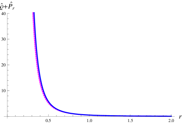
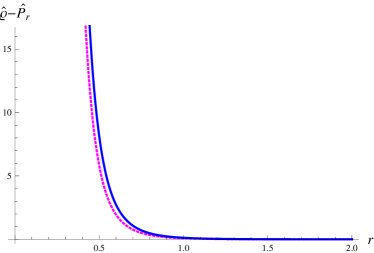
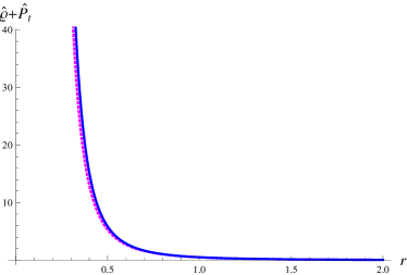
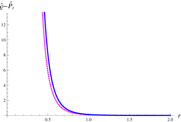
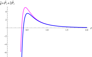
Figure 5: Energy bounds of the interior for $\aleph=2.5$ (Magenta) and $\aleph=3.5$ (Blue).

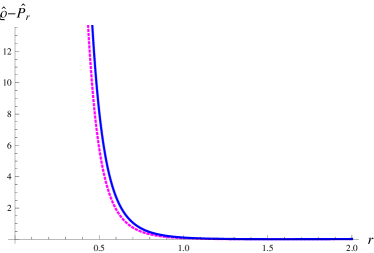
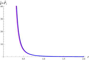
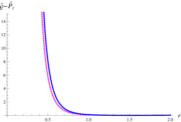
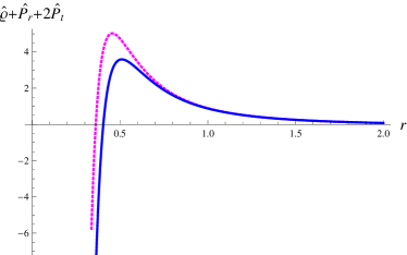
Figure 6: Plots of energy conditions of the exterior for $\aleph=2.5$ (Magenta) and $\aleph=3.5$ (Blue).

5 Concluding Remarks

In this paper, we have constructed anisotropic version of the gravastar in EMSG by employing gravitational decoupling technique. The system of field equations is separated into two different arrays: one belongs to the standard version of $f(\Re,{T}^{2})$ equations, whereas the other involves an additional source. A gravastar solution describing the ultra-compact structure with isotropic matter distribution is used to evaluate the first system. The second set involves four unknowns, i.e., three extra source components of $\tau_{\sigma\gamma}$ and decoupling function $\varsigma(r)$. The second system has been closed by employing the property of gravastars, i.e., $g_{00}=0=g_{11}^{-1}$ at $\mathfrak{R}=2M$ (Schwarzschild limit). This feature provides the deformed radial metric component (48) for $n\geq 2$, which leads to the deformed version of gravastar given by Eqs.(44), (48) and (49)-(51) in EMSG gravity.

For the outer geometry, we have assumed two cases. The first case deals with the standard Schwarzschild geometry whereas the crucial impact of coupling constant $\zeta$ of the theory is observed through a relation of the decoupling parameter $\aleph$. This also ensures the regularity condition which is not found in GR [32], as the smooth matching of the deformed interior with standard Schwarzschild exterior is not allowed by the regularity condition. Secondly, the deformed exterior is smoothly matched with the deformed interior. The density, radial/tagential pressure and anisotropic factor have acceptable behavior (Figures 1 and 2). It is mentioned here that the standard Schwarzschild spacetime has a linear profile while the deformed Schwarzschild metric follows positive increasing trend (Figure 3). The finite positive behavior of metric potentials (Figure 4) has a sharp cusp at the matching point of inner and outer boundaries. We have also discussed viability of the model through energy bounds (Figures 5 and 6) and found that all the energy conditions are satisfied except SEC.

It is worthwhile to mention here that the new version provides an ultra-compact structure that satisfies the requirement of a viable celestial body. Finally, we conclude that the gravastar structure is more compact and stable under the impact of anisotropy in comparison to the related work in other modified theories of gravity using isotropic matter configuration [21]-[29]. Furthermore, our analysis is found to be consistent with GR [20] and curvature-matter coupled theory of gravity [42].

References

- [1] Cognola, G. et al.: Phys. Rev. D 77(2008)046009; Felice, A.D. and Tsujikawa, S.R.: Living Rev. Relativ. 13(2010)3; Nojiri, S. and Odintsov, S.D.: Phys. Rep. 505(2011)59.
- [2] Harko, T. et al.: Phys. Rev. D 84(2011)024020.
- [3] Haghani, Z. et al.: Phys. Rev. D 88(2013)044023.
- [4] Katrici, N. and Kavuk, M.: Eur. Phys. J. Plus 129(2014)163.
- [5] Roshan, M. and Shojai, F.: Phys. Rev. D 94(2016)044002.
- [6] Board, C.V.R. and Barrow, J.D.: Phys. Rev. D 96(2017)123517.
- [7] Nari, N. and Roshan, M.: Phys. Rev. D 98(2018)024031.
- [8] Bahamonde, S., Marciu, M. and Rudra, P.: Phys. Rev. D 100(2019)083511.
- [9] Sharif, M. and Naz, S.: Universe 8(2022)142; Eur. Phys. J. Plus 137(2022)421; Mod. Phys. Lett. A 37(2022)2250125; Int. J. Mod. Phys. D 31(2022)2240008.
- [10] Sharif, M. and Iltaf, S.: Phys. Scr. 97(2022)075002.
- [11] Sharif, M. and Anjum, A.: Eur. Phys. J. Plus 137(2022)602.
- [12] Mazur, P.O. and Mottola, E.: Proc. Natl. Acad. Sci. 101(2004)9545.
- [13] Mottola, E.: Acta Phys. Pol. B 41(2010)2031.
- [14] Mazur, P.O. and Mottola, E.: Class. Quantum Grav. 32(2015)215024).
- [15] Visser, M. and Wiltshire, D.L.: Class. Quantum Grav. 21(2004)1135.
- [16] Carter, B.M.N.: Class. Quantum Grav. 22(2005)4551.
- [17] Cattoen, C., Faber, T. and Visser, M.: Class. Quantum Grav. 22(2005)4189.
- [18] Bilic, N., Tupper, G.B. and Viollier, R.D.: J. Cosmol. Astropart. Phys. 02(2006)013.
- [19] Horvat, D. and Ilijic, S.: Class. Quantum Grav. 24(2007)5637.
- [20] Ovalle, J., Posada, C. and Stuchlik, Z.: Class. Quantum Grav. 36(2019)105010;
- [21] Das, A. et al.: Phys. Rev. D 95(2017)124011.
- [22] Shamir, F. and Ahmad, M.: Phys. Rev. D 97(2018)104031.
- [23] Debnath, U.: Eur. Phys. J. C 79(2019)499.
- [24] Abbas, G. and Majeed, K.: Adv. Astron. 2020(2020)8861168.
- [25] Yousaf, Z., Bhatti, M.Z. and Asad, H.: Phys. Dark Universe 28(2020)100501.
- [26] Bhatti, M.Z. et al.: Phys. Dark Universe 29(2020)100561.
- [27] Ray, S., Sengupta, R., and Nimesh, H.: Int. J. Mod. Phys. D 29(2020)2030004.
- [28] Bhatti, M.Z. et al.: Chin. J. Phys. 73(2021)167; Mod. Phys. Lett. A 36(2021)2150233.
- [29] Bhar, P. and Rej, P.: Eur. Phys. J. C. 81(2021)763.
- [30] Ovalle, J.: Mod. Phys. Lett. A 23(2008)3247; Phys. Rev. D 95(2017)104019.
- [31] Ovalle, J. et al.: Eur. Phys. J. C 78(2018)122.
- [32] Ovalle, J., Posada, S. and Stuchlik, Z.: Class. Quantum Grav. 36(2019)205010.
- [33] Gabbanelli, L., Rincon, A. and Rubio, C.: Eur. Phys. J. C 78(2018)370.
- [34] Graterol, R.P.: Eur. Phys. J. C 133(2018)244.
- [35] Sharif, M. and Sadiq, S.: Eur. Phys. J. C 78(2018)410; Eur. Phys. J. Plus 133(2018)245.
- [36] Morales, E. and Tello-Ortiz, F.: Eur. Phys. J. C 78(2018)841.
- [37] Maurya, S.K., Banerjee, A. and Hansraj, S.: Phys. Rev. D 97(2018)044022.
- [38] Sharif, M. and Majid, A.: Chin. J. Phys. 68(2020)406; Phys. Dark Universe 30(2020)100610.
- [39] Maurya, S.K. et al.: Phys. Dark Universe 30(2020)100640.
- [40] Zubair, M. and Azmat, H.: Eur. Phys. J. Plus 136(2021)112.
- [41] Sharif, M. and Naseer, T.: Chin. J. Phys. 73(2021)179; Universe 8(2022)62.
- [42] Azmat, H., Zubair, M. and Ahmad, Z.: Ann. Phys. 439(2022)168769.