D-SVM over Networked Systems with Non-Ideal Linking Conditions

Abstract

This paper considers distributed optimization algorithms, with application in binary classification via distributed support-vector-machines (D-SVM) over multi-agent networks subject to some link nonlinearities. The agents solve a consensus-constraint distributed optimization cooperatively via continuous-time dynamics, while the links are subject to strongly sign-preserving odd nonlinear conditions. Logarithmic quantization and clipping (saturation) are two examples of such nonlinearities. In contrast to existing literature that mostly considers ideal links and perfect information exchange over linear channels, we show how general sector-bounded models affect the convergence to the optimizer (i.e., the SVM classifier) over dynamic balanced directed networks. In general, any odd sector-bounded nonlinear mapping can be applied to our dynamics. The main challenge is to show that the proposed system dynamics always have one zero eigenvalue (associated with the consensus) and the other eigenvalues all have negative real parts. This is done by recalling arguments from matrix perturbation theory. Then, the solution is shown to converge to the agreement state under certain conditions. For example, the gradient tracking (GT) step size is tighter than the linear case by factors related to the upper/lower sector bounds. To the best of our knowledge, no existing work in distributed optimization and learning literature considers non-ideal link conditions.

1 Introduction

Background: Support-vector-machine (SVM) is a supervised learning method used for classification, regression, and outlier detection cortes1995support ; drucker1996support . Consider a labelled set of given data points each belonging to one of the two classes/labels. The SVM classifies these data and decides which class a new data point belongs to. In the centralized setting, all the data points are available at a central processing node/unit which performs the classification task and finds the SVM parameters. In distributed/decentralized setting (referred to as D-SVM), the data points are distributed among some computing nodes. Every computing node has access to a portion of the data points and computes the associated SVM parameters for classification. Then shares the SVM information over the multi-agent network (that could be subject to nonlinearities) and updates the SVM parameters based on the received information over the network. In this way, the nodes compute the SVM classifiers collaboratively without sharing any data points. The existing works of literature are either (i) centralized and need all the data points at a central processor, or (ii) need the missing data points at all the computing nodes. Both cases require a lot of information sharing and long-distance communication to the central unit (case (i)) or other computing nodes (case (ii)). Also, these may raise privacy concerns due to sharing raw data over the network. The distributed setups (D-SVM), on the other hand, only share SVM data to be updated. Many existing D-SVM solutions consider a linear setup, where the information exchange among the nodes is ideal and linear. However, this data-sharing might be subject to non-ideal linking conditions (e.g., quantization or clipping). This work takes these into consideration by modelling nonlinear linking among the nodes. In general, we assume the data received from one node from another node has gone through a nonlinear channel and this nonlinearity represents any non-ideal linking condition that may exist in the real-world. This gives the most general form of non-ideal linking and to our best knowledge, no existing work in the literature considers such a general solution. This motivates our paper for practical D-SVM and machine learning applications.

Literature Review: This paper extends our previous results on consensus optimization and distributed learning in dsvm to address some practical nonlinearities in real applications. For example, in many machine-learning applications, the data exchange over the network is in discrete-values ecc_mixed and needs to be quantized magnusson2018communication , or in swarm robotic networks the actuators might be subject to saturation ccta22 . These inherent unseen nonlinearities in the real optimization models may result in inaccuracy and unacceptable outcomes, degrading efficiency and increasing the operation costs ccta22 . On the other hand, in some applications, e.g., optimal resource allocation and consensus algorithms, sign-based nonlinearities are added for the purpose of robustness to impulsive noise stankovic2020nonlinear or improving the convergence rate garg2019fixed2 ; my_ecc ; ning2017distributed ; rahili_ren . Many other recent works address different constraints in the distributed optimization framework. For example, in contrast to primary linear models van2019distributed ; nedic2017achieving ; simonetto2017decentralized ; akbari2015distributed ; ling2013decentralized ; wei_me_cdc22 ; koppel2018decentralized ; xi2017add ; forero2010consensus , consensus optimization in a multiple leader containment as in opinion dynamics ecc_containment , under communication constraint and server failure ecc_compres , under mixed-integer value algorithms over computer networks ecc_mixed , and under non-negative constraints on the states (non-negative orthant) ecc_nonnegative are discussed recently.

Contributions: In this work, we assume that the links (over the multi-agent network) are subject to sector-bounded link nonlinear conditions, i.e., the sent information over the transmission links is not linearly delivered; for example, due to (log) quantization or clipping. We show that under strongly sign-preserving odd nonlinearity on the links, the exact convergence to the optimizer can be achieved. Some detailed examples of such nonlinear applications are given in our previous work on resource allocation ccta22 . Similar to van2019distributed ; nedic2017achieving ; simonetto2017decentralized ; akbari2015distributed we prove convergence over (possibly) dynamic networks via a hybrid setup based on matrix perturbation theory and algebraic graph theory. For general strictly convex cost functions, we prove convergence of the nonlinear version of our previously proposed protocol in dsvm over general weight-balanced undirected graphs, which advances the doubly-stochastic assumption in some ADMM-based solutions ling2013decentralized ; wei_me_cdc22 . Note that, in general, weight symmetry (and weight balancing) is easier to satisfy in contrast to weight-stochasticity. This is particularly of interest in packet-drop and link-failure scenarios icrom22_drop which require weight-compensation algorithms for convergence 6426252 ; cons_drop_siam in the existing bi-stochastic network designs. In other words, the existing bi-stochastic networks need compensation algorithms as described in 6426252 ; cons_drop_siam to redesign the network weights after link removal, but the weight-symmetric condition in this work may still hold with no need for redesign algorithms, e.g., in the case of bidirectional link removal. This is discussed in detail for the distributed resource allocation problem in icrom22_drop .

Moreover, we show that the gradient tracking property of our proposed GT-based dynamics holds under additive odd sign-preserving nonlinearities, which is another improvement over ADMM-based solutions. This further allows for, e.g., adding sign-based dynamics to reach faster convergence (in finite/fixed-time taes2020finite ) or to make the solution resilient to outliers, disturbances, and impulsive noise as in some consensus literature stankovic2020nonlinear , but with the drawback of unwanted chattering due to non-Lipschitz continuity at the origin. To the best of our knowledge, such general resiliency to additive linking conditions is not addressed in the existing distributed optimization and learning literature.

Paper organization: Section 2 recaps some preliminaries on algebraic graph theory and perturbation theory. Section 3 formulates the D-SVM as a consensus optimization problem. Section 4 presents our nonlinear GT-based method with its convergence discussed in Section 5. Section 6 gives a simulation on an illustrative example, and Section 7 concludes the paper.

2 Preliminaries

2.1 Notations

${\lVert A\rVert}$ denotes the norm operator on a matrix, i.e., $\lVert A\rVert=\sup_{\lVert\mathbf{x}\rVert=1}\lVert A\mathbf{x}\rVert$. ${\lVert A\rVert_{2}}$ is the spectral norm defined as the square root of the max eigenvalue of $A^{\top}A$, and $\lVert A\rVert_{\infty}=\max_{1\leq i\leq n}\sum_{j=1}^{n}|a_{ij}|$ as the infinity norm. $\sigma(A)$ denotes the eigen-spectrum of $A$ and $\lambda$ denotes the eigenvalue. LHP and RHP respectively imply left-half-plane and right-half-plane in the complex domain. $\partial_{a}z=\frac{dz}{da}$ denotes the derivative with respect to $a$. $\mathbf{1}_{n}$ and $\mathbf{0}_{n}$ are size $n$ vectors of all $1$’s and $0$’s. ‘;’ denotes column vector concatenation. $\nabla_{\mathbf{x}}F$ and $H:=\nabla_{\mathbf{x}}^{2}F$ denote the first and second gradient of $F$ with respect to $\mathbf{x}$. Operators $\prec,\preceq,\succ,\succeq$ denote the element-wise version of $<,\leq,>,\geq$. The identity matrix of size $n$ is denoted by $I_{n}$.

2.2 Recall on Algebraic Graph Theory

We represent the multi-agent network by a strongly-connected undirected graph $\mathcal{G}$ with adjacency matrix $W=\{w_{ij}\}$. $w_{ij}$ is defined as the weight on the link $j\rightarrow i$ and zero otherwise. For an SC $\mathcal{G}$, matrix $W$ is irreducible. The Laplacian matrix $\overline{W}=\{\overline{w}_{ij}\}$ is then defined as $\overline{w}_{ij}=w_{ij}$ for $i\neq j$ and $\overline{w}_{ij}=-\sum_{i=1}^{n}w_{ij}$ for $i=j$.

Lemma 1

SensNets:Olfati04 The Laplacian $\overline{W}$ of a connected weigh-balanced graph has one isolated eigenvalue at zero and the rest on LHP.

A graph is weight-balanced (WB) if the weight-sum of incoming and outgoing links at every node $i$ are equal, i.e., $\sum_{j=1}^{n}w_{ji}=\sum_{j=1}^{n}w_{ij}$.

Lemma 2

SensNets:Olfati04 Given a WB-graph, $W\mathbf{1}_{n}=\mathbf{1}_{n}^{\top}W$, and its Laplacian $\overline{W}$ has the same left and right eigenvectors $\mathbf{1}_{n}^{\top}$ and $\mathbf{1}_{n}$ associated with its zero eigenvalue, i.e., $\mathbf{1}_{n}^{\top}\overline{W}=\mathbf{0}_{n}$ and $\overline{W}\mathbf{1}_{n}=\mathbf{0}_{n}$.

2.3 Auxiliary Results on Perturbation Theory

We recall some results of the matrix perturbation theory.

Lemma 3

stewart_book ; cai2012average Assume an $n$-by-$n$ matrix $P(\alpha)$ which smoothly depends on a real parameter ${\alpha\geq 0}$, and has ${l<n}$ equal eigenvalues $\lambda_{1}=\ldots=\lambda_{l}$, associated with linearly independent right and left unit eigenvectors $\mathbf{v}_{1},\ldots,\mathbf{v}_{l}$ and $\mathbf{u}_{1},\ldots,\mathbf{u}_{l}$. Denote by $\lambda_{i}(\alpha)$, corresponding to ${\lambda_{i},i\in\{1,\ldots,l\}}$, as the eigenvalues of $P(\alpha)$ as a function of independent parameter $\alpha$. Then, $\partial_{\alpha}\lambda_{i}|_{\alpha=0}$ is the $i$-th eigenvalue of the following $l$-by-$l$ matrix, and

$$\left(\begin{array}[]{ccc}\mathbf{u}_{1}^{\top}P^{\prime}\mathbf{v}_{1}&\ldots&\mathbf{u}_{1}^{\top}P^{\prime}\mathbf{v}_{l}\\ &\ddots&\\ \mathbf{u}_{l}^{\top}P^{\prime}\mathbf{v}_{1}&\ldots&\mathbf{u}_{l}^{\top}P^{\prime}\mathbf{v}_{l}\end{array}\right),~{}P^{\prime}=\partial_{\alpha}P(\alpha)|_{\alpha=0}$$

Lemma 4

(bhatia2007perturbation, , Theorem 39.1) Let system matrix ${M(\alpha)=M_{0}+\alpha M_{1}}$, with $\alpha$-independent matrices $M_{0}$ and $M_{1}$. Then, the optimal matching distance satisfies ${d(\sigma(M),\sigma(M_{0}))\leq 4(\lVert M_{0}\rVert+\lVert M\rVert)^{1-\frac{1}{nm}}\lVert\alpha M_{1}\rVert^{\frac{1}{nm}}}$ for ${\min_{\pi}\max_{1\leq i\leq 2nm}(\lambda_{i}-\lambda_{\pi(i)}(\alpha))}$ with $\pi(i)$ as the $i$th permutation over $2mn$ symbols.

3 Problem Statement

3.1 Mathmatical Formulation

Following the notation in dsvm , let $\mathbf{x}=[\mathbf{x}_{1};\mathbf{x}_{2};\dots;\mathbf{x}_{n}]\in\mathbb{R}^{nm}$ represent the column state vector and $\mathbf{x}_{i}\in\mathbb{R}^{m}$ represent the state at agent $i$. The following consensus-constrained distributed optimization problem is considered

$$\min_{\mathbf{x}\in\mathbb{R}^{nm}} F(\mathbf{x})=\sum_{i=1}^{n}f_{i}(\mathbf{x}_{i})$$

subject to $$~{}\mathbf{x}_{1}=\mathbf{x}_{2}=\dots=\mathbf{x}_{n}.$$ (1)

with $f_{i}:\mathbb{R}^{m}\mapsto\mathbb{R}$ as the local cost function at agent/node $i$. Let $\nabla F:\mathbb{R}^{nm}\mapsto\mathbb{R}^{nm}$ denote the gradient of global cost ${F:\mathbb{R}^{nm}\mapsto\mathbb{R}}$. The idea in this work is to solve problem (1) in a distributed way, i.e., locally over a multi-agent network. In this scenario, every agent only uses the local information in its neighbourhood (and its own information) to solve (1).We assume that problem (1) is proper and well-defined and there exists $\overline{\mathbf{x}}^{*}\in\mathbb{R}$ such that ${\nabla F(\mathbf{x}^{*})=\mathbf{0}_{n}}$. Then, the optimizer of (1) is defined as $\mathbf{x}^{*}:=[\mathbf{x}^{*}_{1};\mathbf{x}^{*}_{2};\dots;\mathbf{x}^{*}_{n}]=\overline{\mathbf{x}}^{*}\mathbf{1}_{n}$ which satisfies ${\sum_{i=1}^{n}\partial_{x_{i}}f_{i}(\mathbf{x}^{*}_{i})=0}$.

Remark 1

Other equivalent formulations of the consensus-constraint problem (1) are also discussed in the literature. In gharesifard2013distributed , problem (1) is shown to be equivalent with general unconstrained formulation,

$$\min_{\mathbf{x}\in\mathbb{R}^{m}} F(\mathbf{x})=\sum_{i=1}^{n}f_{i}(\mathbf{x})$$ (2)

or its Laplacian-constraint version as,

$$\min_{\mathbf{x}\in\mathbb{R}^{nm}} F(\mathbf{x})=\sum_{i=1}^{n}f_{i}(\mathbf{x}_{i})$$

subject to $$~{}\mathcal{L}\mathbf{x}=\mathbf{0}_{nm}.$$ (3)

with $\mathcal{L}=L\otimes I_{m}$ and $L$ as the Laplacian of the weight-balanced graph $\mathcal{G}$.

Assumption 1

Each local cost $f_{i}$ is strictly convex with smooth gradient and positive-definite (PD) $\nabla^{2}f_{i}(\mathbf{x}_{i})$.

Under Assumption 1, the unique optimizer of (1) is in the form $\mathbf{x}^{*}=\mathbf{1}_{n}\otimes\overline{\mathbf{x}}^{*}$ with $\overline{\mathbf{x}}^{*}\in\mathbb{R}^{m}$.

3.2 Application in D-SVM

We recall here a specific application of problem (1) given in dsvm for distributed support-vector-machines (D-SVM). Consider binary classification using a given training set of data points ${\boldsymbol{\chi}_{i}\in\mathbb{R}^{m-1}}$, ${i=1,\ldots,N}$, each labelled by ${l_{i}\in\{-1,1\}}$. The standard (centralized) SVM problem finds the optimal max-margin classifier ${\boldsymbol{\omega}^{\top}\boldsymbol{\chi}-\nu=0}$ (as a hyperplane) to partition the data points into two classes in $\mathbb{R}^{m-1}$. The hyperplane parameters $\boldsymbol{\omega}~{}$ and $\nu$ are optimal solution to the following minimization problem chapelle2007training :

$$\begin{aligned} \displaystyle&\min_{\boldsymbol{\omega},\nu}~{}&\boldsymbol{\omega}^{\top}\boldsymbol{\omega}+C\sum_{j=1}^{N}\max\{1-l_{j}(\boldsymbol{\omega}^{\top}\phi(\boldsymbol{\chi}_{j})-\nu),0\}^{p}\end{aligned}$$ (4)

with ${p=\{1,2,\ldots\}}$ and $C$ respectively as the smoothness and margin-size parameters. Given the parameters $\boldsymbol{\omega},\nu$ of the separating hyperplane, a test data point $\widehat{\boldsymbol{\chi}}$ is labeled (classified) by ${g(\widehat{\boldsymbol{\chi}})=\text{sgn}(\boldsymbol{\omega}^{\top}\widehat{\boldsymbol{\chi}}-\nu)}$. The notions of nonlinear mapping $\phi(\cdot)$ associated with a kernel function $K(\boldsymbol{\chi}_{i},\boldsymbol{\chi}_{j})=\phi(\boldsymbol{\chi}_{i})^{\top}\phi(\boldsymbol{\chi}_{j})$ can further be used to project the data points into a high-dimensional space $\mathcal{F}$ in which the data points are linearly separable such that ${g(\widehat{\boldsymbol{\chi}})=\text{sgn}(\boldsymbol{\omega}^{\top}\phi(\widehat{\boldsymbol{\chi}})-\nu)}$ determines the class of $\widehat{\boldsymbol{\chi}}$. Recall that, as a standard convention, the non-differentiable function $\max\{z,0\}^{p}$ for ${p=1}$ in SVM formulation (4) is replaced by the twice differentiable ${L(z,\mu)=\frac{1}{\mu}\log(1+\exp(\mu z))}$ (hing loss model garg2019fixed2 ; slp_book ). It can be shown that by setting $\mu$ large enough ${L(z,\mu)}$ becomes arbitrarily close to $\max\{z,0\}$ slp_book ; dsvm .

In D-SVM setup, the data points are distributed among $n$ agents each with $N_{i}$ data points denoted by $\boldsymbol{\chi}^{i}_{j},{j=1,\ldots,N_{i}}$. The trivial solution is that agents share some data points (the support vectors) locally which raises data-privacy concerns navia2006distributed . The more recent idea is to find a distributed learning mechanism such that no agent reveals its local (support vector) data to any other agent or over non-private communication channels dsvm . Each agent $i$ solves (4) and finds its local classifier parameters $\boldsymbol{\omega}_{i}$ and $\nu_{i}$ based on its partial dataset $\boldsymbol{\chi}^{i}_{j},{j=1,\ldots,N_{i}}$, which in general differs from other agents. This is done by formulating the problem into the general distributed optimization format as given by (1),

$$\begin{aligned} \displaystyle\min_{\boldsymbol{\omega}_{1},\nu_{1},\ldots,\boldsymbol{\omega}_{n},\nu_{n}}\quad&\sum_{i=1}^{n}\boldsymbol{\omega}_{i}^{\top}\boldsymbol{\omega}_{i}+C\sum_{j=1}^{N_{i}}\tfrac{1}{\mu}\log(1+\exp(\mu z))\\ \text{subject to}\quad&\boldsymbol{\omega}_{1}=\dots=\boldsymbol{\omega}_{n},\qquad\nu_{1}=\dots=\nu_{n},\end{aligned}$$ (5)

with hing loss function ${f_{i}:\mathbb{R}^{m}\mapsto\mathbb{R}}$ locally defined at each agent $i$. The consensus constraint in (5) ensures that agents learn (and reach an agreement on) the overall classifier parameters $\boldsymbol{\omega}$ and $\nu$.

4 Proposed Dynamics subject to Link Nonlinearity

4.1 The Linear Setup

To solve problem (1), we previously proposed the following GT-based linear dynamics in dsvm .

$$\dot{\mathbf{x}}_{i} =-\sum_{j=1}^{n}w_{ij}^{q}(\mathbf{x}_{i}-\mathbf{x}_{j})-\alpha\mathbf{y}_{i},$$ (6)

$$\dot{\mathbf{y}}_{i} =-\sum_{j=1}^{n}a_{ij}^{q}(\mathbf{y}_{i}-\mathbf{y}_{j})+\partial_{t}\nabla f_{i}(\mathbf{x}_{i}),$$ (7)

with $\mathbf{x}_{i}(t)$ as the state of agent $i$ at time ${t\geq 0}$, ${\mathbf{y}=[\mathbf{y}_{1};\mathbf{y}_{2};\dots;\mathbf{y}_{n}]\in\mathbb{R}^{mn}}$ as the auxiliary variable tracking the sum of local gradients, and the matrix ${A_{q}=\{a_{ij}^{q}\}},{W_{q}=\{w_{ij}^{q}\}}$ as the WB adjacency matrices of $\mathcal{G}_{q}$ ($q$ as possible switching signal), and $\alpha>0$ as the GT step-size. The compact formulation of (6)-(7) is

$$\left(\begin{array}[]{c}\dot{\mathbf{x}}\\ \dot{\mathbf{y}}\end{array}\right) =M(t,\alpha,q)\left(\begin{array}[]{c}{\mathbf{x}}\\ {\mathbf{y}}\end{array}\right),$$ (12)

$$M(t,\alpha,q) =\left(\begin{array}[]{cc}\overline{W}_{q}\otimes I_{m}&-\alpha I_{mn}\\ H(\overline{W}_{q}\otimes I_{m})&\overline{A}_{q}\otimes I_{m}-\alpha H\end{array}\right).$$ (15)

with Hessian matrix $H:=\text{blockdiag}[\nabla^{2}f_{i}(\mathbf{x}_{i})]$. Note that the linear networked dynamics (12)-(15) and its nonlinear counterpart in the next section represent hybrid dynamical systems because the matrix $H$ (and parameter $\Xi(t)$ in the upcoming nonlinear case (16)-(34)) varies in continuous-time and the structure of the Laplacians $\overline{W}_{q}$ and $\overline{A}_{q}$ may switch in discrete-time via a switching signal $q$ (as a dynamic network topology). We assume that this signal $q$ as the jump map satisfies the assumptions for stability and regularity conditions as discussed in goebel2009hybrid ; sam_tac:17 . We skip the details due to space limitations and refer interested readers to our previous work (dsvm, , footnote 1) for more discussions on this.

4.2 The Nonlinear Setup

Next, we consider possible nonlinearities at the linking between agents, denoted by nonlinear mapping $g:\mathbb{R}^{m}\mapsto\mathbb{R}^{m}$. Then, (6)-(7) is reformulated as

$$\dot{\mathbf{x}}_{i} =-\sum_{j=1}^{n}w_{ij}^{q}(g(\mathbf{x}_{i})-g(\mathbf{x}_{j}))-\alpha\mathbf{y}_{i},$$ (16)

$$\dot{\mathbf{y}}_{i} =-\sum_{j=1}^{n}a_{ij}^{q}(g(\mathbf{y}_{i})-g(\mathbf{y}_{j}))+\partial_{t}\nabla f_{i}(\mathbf{x}_{i}),$$ (17)

Assumption 2

The nonlinear mapping $g(\cdot)$ is odd, sign-preserving, and monotonically non-decreasing. Further, $g$ is upper/lower sector-bounded by positive parameters $\kappa,\mathcal{K}>0$, i.e., $0<\kappa\leq\frac{g(z)}{z}\leq\mathcal{K}$, where the parameters $\kappa,\mathcal{K}$ satisfy the frequency condition in circle criterion.

In compact form at every operating time $t$, one can rewrite the dynamics (16)-(17) as

$$\left(\begin{array}[]{c}\dot{\mathbf{x}}\\ \dot{\mathbf{y}}\end{array}\right)=M_{g}(t,\alpha,q)\left(\begin{array}[]{c}{\mathbf{x}}\\ {\mathbf{y}}\end{array}\right),$$ (22)

$$M_{g}(t,\alpha,q)=\left(\begin{array}[]{cc}\overline{W}_{q,\Xi}\otimes I_{m}&-\alpha I_{mn}\\ H(\overline{W}_{q,\Xi}\otimes I_{m})&\overline{A}_{q,\Xi}\otimes I_{m}-\alpha H\end{array}\right).$$ (25)

where $M_{g}(t,\alpha,q)$ represents the linearization at every operating point $t$, which is also a function of the parameter $\alpha$ and a switching signal $q$ of the network (to be described later). In the linear case as in dsvm with $g(z)=z$, one can formulate the above as $M=M^{0}+\alpha M^{1}$ with

$$M^{0} = \left(\begin{array}[]{cc}\overline{W}_{q}\otimes I_{m}&\mathbf{0}_{mn\times mn}\\ H(\overline{W}_{q}\otimes I_{m})&\overline{A}_{q}\otimes I_{m}\end{array}\right),$$ (28)

$$M^{1} = \left(\begin{array}[]{cc}\mathbf{0}_{mn\times mn}&-{I_{mn}}\\ {\mathbf{0}_{mn\times mn}}&-H\end{array}\right),$$ (31)

Then, in the nonlinear case of this paper, one can rewrite the compact formulation of (22)-(25) as,

$$M_{g}(t,\alpha,q) =M_{g}^{0}+\alpha M^{1}$$ (32)

$$\kappa M^{0} \preceq M_{g}^{0}\preceq\mathcal{K}M^{0}$$ (33)

$$M_{g}^{0}=\Xi(t)M^{0} ,~{}\kappa I_{n}\preceq\Xi(t)\preceq\mathcal{K}I_{n}$$ (34)

with $\Xi(t)=\mbox{diag}[\xi(t)]$, $\xi(t)=[\xi_{1}(t);\xi_{2}(t);\dots;\xi_{n}(t)]$, and $\xi_{i}(t)=\frac{g(\mathbf{x}_{i})}{\mathbf{x}_{i}}$. Note that, from Assumption 2, $\kappa\leq\xi_{i}(t)\leq\mathcal{K}$, and we have $\overline{W}_{q,\Xi}=\overline{W}_{q}\Xi(t)$, $\overline{A}_{q,\Xi}=\overline{A}_{q}\Xi(t)$ as one can write (with a slight abuse of notation) $g(\mathbf{x}(t))=\Xi(t)\mathbf{x}(t)$.

Remark 2

To relate $\sigma(\overline{W}_{q,\Xi})$ and $\sigma(\overline{W}_{q})$, note that $\mbox{det}(\overline{W}_{q,\Xi}-\lambda I_{2mn})=\mbox{det}(\overline{W}_{q}-\lambda\Xi(t)^{-1})$ since $\Xi(t)$ is a diagonal matrix.

In the rest of this paper, for notation simplicity, we drop the dependence on $(t,\alpha,q)$ unless where needed.

Assumption 3

The network is connected and undirected (bidirectional links) with non-negative weights ${W_{q}=\{w_{ij}^{q}\}}$ and ${A_{q}=\{a_{ij}^{q}\}}$. Further, $\sum_{j=1}^{n}w_{ij}^{q}<1$ and  ${\sum_{j=1}^{n}a_{ij}^{q}<1}$ with $q$ denoting the switching signal in hybrid mode.

Assumptions 2-3 guarantee that under (16) and (17):

$$\sum_{i=1}^{n}\dot{\mathbf{y}}_{i}=\sum_{i=1}^{n}\partial_{t}\nabla f_{i}(\mathbf{x}_{i}),~{}~{}\sum_{i=1}^{n}\dot{\mathbf{x}}_{i}=-\alpha\sum_{i=1}^{n}\mathbf{y}_{i}.$$ (35)

which can be proved similar to the proof of (my_ecc, , Lemma 3). Initializing the auxiliary variable $\mathbf{y}(0)=\mathbf{0}_{nm}$ it can be also seen that, similar to the linear case (6)-(7) dsvm , we have

$$\sum_{i=1}^{n}\dot{\mathbf{x}}_{i}=-\alpha\sum_{i=1}^{n}\mathbf{y}_{i}=-\alpha\sum_{i=1}^{n}\nabla f_{i}(\mathbf{x}_{i}),$$ (36)

and the time-derivative of $\sum_{i=1}^{n}\mathbf{x}_{i}$ (the sum of states) moves towards the summed gradient. Note that the same set of equations holds for linear case (16)-(17). This follows from the structure of our GT-based protocol that allows for odd sign-preserving nonlinearities to be embedded in the model without disrupting the gradient tracking dynamics. This particularly is an improvement over existing ADMM-based dynamics, e.g., ling2013decentralized . Then, one can show that for any initialization $\mathbf{x}(0)\notin\mbox{span}\{\mathbf{1}_{n}\otimes\varphi\}$ and $\mathbf{y}(0)=\mathbf{0}_{nm}$, from (36), and due to the strict convexity of $F(\mathbf{x})$, the following uniquely holds at ${\mathbf{x}=\mathbf{x}^{*}=\mathbf{1}_{n}\otimes\overline{\mathbf{x}}^{*}}$,

$$\sum_{i=1}^{n}\dot{\mathbf{x}}_{i}=-\alpha(\mathbf{1}_{n}^{\top}\otimes I_{m})\nabla F(\mathbf{x}^{*})=\mathbf{0}_{m}.$$

Further, from (6) we have $\dot{\mathbf{x}}_{i}=\mathbf{0}_{m}$ and from (7),

$$\dot{\mathbf{y}}_{i}=\partial_{t}\nabla f_{i}(\overline{\mathbf{x}}^{*})=\nabla^{2}f_{i}(\overline{\mathbf{x}}^{*})\dot{\mathbf{x}}_{i}=\mathbf{0}_{m},$$

which shows that the state $[\mathbf{x}^{*};\mathbf{0}_{nm}]$ with $(\mathbf{1}_{n}^{\top}\otimes I_{m})\nabla F(\mathbf{x}^{*})=\mathbf{0}_{m}$ is an invariant equilibrium point of both linear dynamics (6)-(7) and nonlinear dynamics (16)-(17) satisfying Assumption 2.

5 Convergence Analysis via Perturbation Theory

To prove the convergence to the optimizer $\mathbf{x}^{*}$ under the proposed GT-based nonlinear (hybrid) setup, we show the stability of the matrix $M_{g}$ at every time-instant using the matrix perturbation theory stewart_book . Recall that the stability of a nonlinear system can be analyzed by addressing its stability at every operating point (over time) nonlin ; Liu-nature . In this direction, we specifically show that the algebraic multiplicity of zero eigenvalues of $M_{g}$ is $m$ (at all times $t>0$) while the remaining eigenvalues are in the LHP. For this part, unlike existing literature with strong convexity condition van2019distributed ; nedic2017achieving ; ling2013decentralized ; simonetto2017decentralized ; akbari2015distributed ; koppel2018decentralized , we only assume strict convexity (Assumption 1). We also show that the convergence rate of the solution and its associated Lyapunov function depend on the largest non-zero eigenvalue of $M_{g}$ in the LHP; and, following the continuity of the Lyapunov function at the jump points, the convergence over the entire (hybrid) time horizon can be proved nonlin ; goebel2009hybrid .

Theorem 1

Let Assumptions 1-3 hold. At every iteration point $\forall t>0$, the matrix $M_{g}$ given by (25) has only one set of zero eigenvalues with algebraic multiplicity $m$.

Proof

The proof follows similar to (dsvm, , Theorem 1) for linear dynamics (6)-(7). For the nonlinear case (16)-(17) we have $M_{g}=M^{0}_{g}+\alpha M^{1}$, and the eigen-spectrum follows as

$$\kappa\sigma(M^{0})\leq\sigma(M^{0}_{g})\leq\mathcal{K}\sigma(M^{0})$$ (37)

where $\sigma(M^{0})=\sigma(\overline{W}\otimes I_{m})\cup\sigma(\overline{A}\otimes I_{m})$, and, from Lemma 1, matrix $M^{0}$ has $m$ eigenvalues associated with $m$ dimensions of vector states $\mathbf{x}_{i}$, i.e.,

$$\operatorname{Re}\{\lambda_{2n,j}\}\leq\ldots\leq\operatorname{Re}\{\lambda_{3,j}\}<\lambda_{2,j}=\lambda_{1,j}=0,$$

where $j=\{1,\ldots,m\}$. We check the spectrum variation under (37) by adding the (small) perturbation $\alpha M_{1}$. In simple words, we want to see whether the zero eigenvalues $\lambda_{1,j}$ and $\lambda_{2,j}$ and other LHP eigenvalues of $M_{0}$ move to the RHP or not (see Fig. 1). Denote these perturbed eigenvalues by $\lambda_{1,j}(\alpha,t)$ and $\lambda_{2,j}(\alpha,t)$ which satisfy (37). Following the results in Section 2.3, we find the right eigenvectors corresponding to $\lambda_{1,j}$ and $\lambda_{2,j}$ of $M^{0}$ as,

$$V=[V_{1}~{}V_{2}]=\frac{1}{\sqrt{n}}\left(\begin{array}[]{cc}\mathbf{1}_{n}&\mathbf{0}_{n}\\ \mathbf{0}_{n}&\mathbf{1}_{n}\end{array}\right)\otimes I_{m},$$ (40)

and the left eigenvectors as $V^{\top}$ using Lemma 2. Note that $V^{\top}V=I_{2mn}$. Then, since $\Xi$ is a diagonal vector, the associated ones with $M_{g}^{0}$ are

$$V_{g}=[V_{g1}~{}V_{g2}]=\left(\begin{array}[]{cc}\mathbf{1}_{n}&\mathbf{0}_{n}\\ \mathbf{0}_{n}&\mathbf{1}_{n}\end{array}\right)\otimes I_{m},$$ (43)

as the right eigenvectors and the same $V^{\top}$ as the left eigenvectors. This follows from Remark 2. From (25), $\partial_{\alpha}M_{g}(\alpha)|_{\alpha=0}=M_{1}$ with $M_{1}$ independent of the nonlinearity $g(\cdot)$. Then, from Lemma 3,

$$V^{\top}M_{1}V_{g}=\left(\begin{array}[]{cc}\mathbf{0}_{m\times m}&\mathbf{0}_{m\times m}\\ \times&-(\mathbf{1}_{n}\otimes I_{m})^{\top}H(\mathbf{1}_{n}\otimes I_{m})\end{array}\right).$$ (46)

From Assumption 1 and 2,

$$-(\mathbf{1}_{n}\otimes I_{m})^{\top}H(\mathbf{1}_{n}\otimes I_{m})=-\sum_{i=1}^{n}\nabla^{2}f_{i}(\mathbf{x}_{i})\prec 0,$$ (47)

From Lemma 3 $\partial_{\alpha}\lambda_{1,j}|_{\alpha=0}$ and $\partial_{\alpha}\lambda_{2,j}|_{\alpha=0}$ depend on the eigenvalues of $V^{\top}M_{1}V_{g}$ in (46). This matrix is lower triangular with $m$ zero eigenvalues and $m$ negative eigenvalues (from (47)). Therefore, ${\partial_{\alpha}\lambda_{1,j}|_{\alpha=0}=0}$ and ${\partial_{\alpha}\lambda_{2,j}|_{\alpha=0}<0}$, i.e., the perturbation $\alpha M_{1}$ moves the $m$ zero eigenvalues $\lambda_{2,j}(\alpha,t)$ of $M_{g}$ toward the LHP while other $m$ zero eigenvalues $\lambda_{1,j}(\alpha,t)$ remain zero. This completes the proof.

Corollary 1

Note that Eq. (46)-(47) in the proof of Theorem 1 are a function of the left and right eigenvectors of $\overline{W}_{q}$ and $\overline{A}_{q}$ (associated with the zero eigenvalue) and the $H$ matrix of the cost function. Given a PD $H$ matrix with $\nabla^{2}f_{i}(\mathbf{x}_{i})\succ 0$ (from Assumption 1), any set of non-negative vectors $V^{\top},V_{g}$ with $\sum_{i=1}^{n}v_{i}v_{g,i}>0$ satisfies Eq. (47). Therefore, the stability results in Theorem 1 hold for any Laplacian matrix whose (left-right) eigenvectors $V^{\top},V_{g}$ satisfy $v_{i}v_{g,i}\geq 0,\forall i$ and $\sum_{i=1}^{n}v_{i}v_{g,i}>0$. In case of homogeneous quadratic costs (i.e., $H=\gamma I$) this sufficient condition simplifies to only $\sum_{i=1}^{n}v_{i}v_{g,i}>0$.

Some relevant discussions to Corollary 1 are given in (SensNets:Olfati04, , Corollary 2) on weighted-average consensus.

Figure 1: This figure illustrates the eigenvalue perturbation analysis in the proof of Theorem 1 with $d(\sigma(M_{g}),\sigma(M_{g}^{0}))$ as the optimal matching distance and $\kappa\lambda_{3,j}(\alpha,t)$ as the maximum negative eigenvalue of $M_{g}^{0}$. For this example, we assume $\lambda_{3,j}(\alpha,t)$ is real-valued.

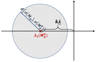
Next, the following finds the bound on $\alpha$ such that other eigenvalues of $M_{g}^{0}$ under perturbation $M_{1}$ remain on the LHP; this is better illustrated in Fig. 1.

In dsvm , we found a bound on $\alpha$ for the linear case, which we recalculate here for the nonlinear case. Let ${\gamma=\max_{1\leq i\leq nm}\sum_{j=1}^{nm}|H_{ij}|}$ and ${\underline{\lambda}=\min_{1\leq j\leq m}|\operatorname{Re}\{\lambda_{3,j}\}|}$ with $\lambda_{3,j}\in\sigma(M^{0})$. From (34) (and (37)), we have $\kappa\underline{\lambda}\leq|\operatorname{Re}\{\lambda_{3,j}(\alpha,t)\}|$, and for eigenvalues of $M_{g}^{0}$ to remain in the LHP we need $d(\sigma(M_{g}),\sigma(M^{0}_{g}))<\kappa\underline{\lambda}$. Then, from Lemma 4 and Fig. 1, the optimal matching distance $d(\sigma(M_{g}),\sigma(M^{0}_{g}))<\kappa\underline{\lambda}$ (i.e., the real parts of the eigenvalues ${\operatorname{Re}\{\lambda_{3,j}(\alpha,t)\},\ldots,\operatorname{Re}\{\lambda_{2n,j}(\alpha,t)\}}$ of $M^{0}_{g}$ are negative) for $0<\alpha<\overline{\alpha}_{g}$ with $\overline{\alpha}_{g}$ defined as

$$\overline{\alpha}_{g} =\operatorname*{argmin}_{\alpha>0}\big{(}|4(2\mathcal{K}+2\gamma$$

$$+\max\{2\mathcal{K}+\gamma(2\mathcal{K}+\alpha),2\mathcal{K}+\alpha\}^{1-\frac{1}{nm}}\alpha^{\frac{1}{nm}}-\kappa\underline{\lambda}|\big{)},$$ (48)

for $\gamma<1$ and,

$$\overline{\alpha}_{g}=\operatorname*{argmin}_{\alpha>0}|4(4\mathcal{K}+\gamma(4\mathcal{K}+\alpha))^{1-\frac{1}{nm}}(\alpha\gamma)^{\frac{1}{nm}}-\kappa\underline{\lambda}.|.$$ (49)

for $\gamma\geq 1$. These are defined based on $\lVert\cdot\rVert_{\infty}$ norm and Assumptions 3 and 1 which gives $\lVert M_{g}^{0}\rVert_{\infty}\leq 2\mathcal{K}(1+\gamma)$, $\lVert\alpha M^{1}\rVert_{\infty}\leq\alpha\max\{\gamma,1\}$, and thus, $\lVert M_{g}\rVert_{\infty}\leq\max\{2\mathcal{K}+\gamma(2\mathcal{K}+\alpha),2\mathcal{K}+\alpha\}$.

Substituting spectral norm in Lemma 4, gives a more intuitive bound for the nonlinear case, which follows from

$$4(\rVert M_{0}^{g}\lVert_{2}+\rVert M^{g}\lVert_{2})^{1-\frac{1}{nm}}\alpha^{\frac{1}{nm}}\rVert M_{1}\lVert_{2}^{\frac{1}{nm}}<\kappa\underline{\lambda},$$ (50)

Assuming the admissible $\alpha$ such that the above holds, $\rVert M\lVert_{2}$ with respect to $\rVert M_{0}\lVert_{2}$ is (at most) perturbed by $\underline{\lambda}$, and from (37) we get

$$4\mathcal{K}^{1-\frac{1}{nm}}(|\lambda_{2nm}|+|\lambda_{2nm}|+\underline{\lambda})^{1-\frac{1}{nm}}\alpha^{\frac{1}{nm}}\max\{1,\gamma\}^{\frac{1}{nm}}<\kappa\underline{\lambda},$$

which gives

$$\overline{\alpha}_{g}\leq\frac{(\kappa\underline{\lambda})^{nm}}{4^{nm}\mathcal{K}^{nm-1}(2|\lambda_{2nm}|+\kappa\underline{\lambda})^{nm-1}\max\{1,\gamma\}}$$ (51)

This gives an intuition on how the (sector-bound) ratio $\frac{\kappa}{\mathcal{K}}<1$ of the nonlinear mapping and the eigen-ratio $\frac{\underline{\lambda}}{|\lambda_{2nm}|}<1$ affect $\overline{\alpha}_{g}$ and the admissible range of ${\alpha}$. Under certain assumptions as in xi2017add , one may find tighter bounds on the step-size $\alpha$. We first use the spectrum analysis in (delay_est, , Appendix) to find the spectrum of $M_{g}(t,\alpha,q)$ in (25). By proper row/column permutations in (delay_est, , Eq. (18)), $\sigma(M_{g})$ follows from

$$\mbox{det}( \alpha I_{mn})\mbox{det}(H(\overline{W}_{q,\Xi}\otimes I_{m})+$$

$$(\overline{A}_{q,\Xi}\otimes I_{m}-\alpha H-\lambda I_{mn})(\frac{1}{\alpha})(\overline{W}_{q,\Xi}\otimes I_{m}-\lambda I_{mn}))=0.$$ (52)

We want to see whether any $\lambda\in\{\sigma(M^{0}_{g})\backslash 0\}$ satisfies the above for an $\alpha$ value. To simplify the analysis, we consider one-component state ($m=1$). Then,

$$\det(\alpha H\overline{W}_{q,\Xi} +\overline{A}_{q,\Xi}\overline{W}_{q,\Xi}-\alpha H\overline{W}_{q,\Xi}-\lambda\overline{W}_{q,\Xi}$$

$$-\lambda\overline{A}_{q,\Xi}+\alpha\lambda H+\lambda^{2}I_{n})=0$$ (53)

which simplifies to

$$\det((\overline{W}_{q,\Xi}-\lambda I_{n})(\overline{A}_{q,\Xi}-\lambda I_{n})+\alpha\lambda H)=0$$

Similar to the proof of Theorem 1, for stability we need to find the admissible range of $\alpha$ values for which the eigenvalues $\sigma(M_{g})$ remain in LHP, except one isolated zero eigenvalue. We recall that the eigenvalues are continuous functions of the matrix elements stewart_book . Therefore, we find the roots of the above (say $\alpha=0$ and $\alpha=\overline{\alpha}_{g}$) for which we have more than one zero eigenvalue. Note that, for $\alpha=0$, $\mbox{det}((\overline{W}_{q,\Xi}-\lambda I_{n})(\overline{A}_{q,\Xi}-\lambda I_{n}))=0$ gives the eigen-spectrum as $\sigma(\overline{A}_{q,\Xi})\cup\sigma(\overline{W}_{q,\Xi})$ with two zero eigenvalues. To find $\overline{\alpha}_{g}$, let assume the same adjacency matrix in (16) and (17) to simplify the problem (i.e., $w^{q}_{ij}=a^{q}_{ij}$). Then,

$$\mbox{det}((\overline{W}_{q,\Xi}-\lambda I_{n})^{2}+\alpha\lambda H)=0$$

Note that the first term gives the eigenvalues of $\overline{W}_{q,\Xi}$ (in the LHP). Since $\alpha H$ is a diagonal matrix one can re-write the above (with some abuse of notation) as

$$\mbox{det}((\overline{W}_{q,\Xi}-\lambda I_{n}+\sqrt{\alpha|\lambda|H})(\overline{W}_{q}-\lambda I_{n}-\sqrt{\alpha|\lambda|H}))=0$$ (54)

which simplifies to

$$\mbox{det}(\overline{W}_{q,\Xi}-\lambda(I_{n}\pm\sqrt{\frac{\alpha H}{|\lambda|}}))=0$$ (55)

This simply means that the eigenvalues are perturbed towards the RHP by the factor of $\sqrt{\frac{\alpha H}{|\lambda|}}$ (or adding the value $\sqrt{\alpha|\lambda|H}$). Therefore, the other root value follows from $\lambda I_{n}=\sqrt{\alpha|\lambda|H}$. In the linear case, one can claim that $\alpha_{g}=\operatorname*{argmin}_{\alpha}|1-\sqrt{\frac{\alpha H}{|\lambda|}}|\geq\frac{\min\{|\lambda|\neq 0\}}{\max\{\partial^{2}f_{i}\}}=\frac{|\lambda_{2}|}{\gamma}$ for $H\preceq\gamma I_{n}$ with $\lambda_{2}$ as the second largest eigenvalue of $M^{0}$. For the nonlinear case, recalling $\overline{W}_{q,\Xi}=\overline{W}_{q}\Xi(t)$,

$$\mbox{det}((\overline{W}_{q}-\lambda I_{n}\Xi(t)^{-1}\pm\sqrt{\alpha|\lambda|H}\Xi(t)^{-1}))=0$$ (56)

which gives $\alpha_{g}\geq\min\{\frac{\kappa|\lambda_{2}|}{\gamma},\frac{|\lambda_{2}|}{\mathcal{K}\gamma}\}$. This implies that, from perturbation analysis as in the proof of Theorem 1, one can claim for max bound on $\overline{\alpha}_{g}$ as

$$\overline{\alpha}_{g}\leq\min\{\frac{\kappa|\lambda_{2}|}{\gamma},\frac{|\lambda_{2}|}{\mathcal{K}\gamma}\}$$ (57)

other $n-1$ eigenvalues of $M_{g}$ are in the LHP. This gives the admissible range to ensure stability. This is used in the next theorem.

Theorem 2

Let Assumptions 1-3 hold. For sufficiently small $0<\alpha_{g}<\overline{\alpha}_{g}$, the proposed nonlinear dynamics (16)-(17) converges to $[\mathbf{x}^{*};\mathbf{0}_{nm}]$ with optimizer $\mathbf{x}^{*}$ as the solution to (1).

Proof

The proof follows from Theorems 1, circle criterion, and the admissible range of $\alpha$ for which all the eigenvalues of $M_{g}$ have non-positive real-parts, $\forall t,q$, and the algebraic multiplicity of zero eigenvalue is $m$. Note that for the circle criterion $A=M^{1}$, $C=M^{0}_{g}$, $\kappa\mathbf{v}\leq\phi(\mathbf{v},t)\leq\mathcal{K}\mathbf{v}$. Then the proof of stability follows from Lyapunov-type analysis similar to dsvm ; define the positive-definite Lyapunov function ${V(\boldsymbol{\delta})=\frac{1}{2}\boldsymbol{\delta}^{\top}\boldsymbol{\delta}=\frac{1}{2}\lVert\boldsymbol{\delta}\rVert_{2}^{2}}$ with residual $\boldsymbol{\delta}=[\mathbf{x};\mathbf{y}]-[\mathbf{x}^{*};\mathbf{0}_{mn}]\in\mathbb{R}^{2mn}$, i.e., the difference of the system state and the optimal state at every time. Recall that $[\mathbf{x}^{*};\mathbf{0}_{nm}]$ is an invariant state of the proposed dynamics and

$${\dot{\boldsymbol{\delta}}=[\dot{\mathbf{x}};\dot{\mathbf{y}}]-[\dot{\mathbf{x}}^{*};\mathbf{0}_{mn}]}={M_{g}([\mathbf{x};\mathbf{y}]-[\mathbf{x}^{*};\mathbf{0}_{mn}])=M_{g}\boldsymbol{\delta}}$$

where $M_{g}[\mathbf{x}^{*};\mathbf{0}_{mn}]=\mathbf{0}_{2mn}$. Then, at every operating point $t>0$ the derivative satisfies ${\dot{V}=\boldsymbol{\delta}^{\top}\dot{\boldsymbol{\delta}}=\boldsymbol{\delta}^{\top}M_{g}\boldsymbol{\delta}}$. Since only ${{\lambda}_{1,j}(\alpha,t)=0}$, while other eigenvalues are in LHP, i.e., ${Re\{{\lambda}_{i,j}(\alpha,t)\}<0}$, for ${2\leq i\leq 2n,1\leq j\leq m}$, one can show that,

$$\boldsymbol{\delta}^{\top}M_{g}\boldsymbol{\delta}\leq\max_{1\leq j\leq m}\operatorname{Re}\{{\lambda}_{2,j}(\alpha,t)\}\boldsymbol{\delta}^{\top}\boldsymbol{\delta}.$$ (58)

where $\lambda_{2,j}(\alpha,t)$ denotes the largest nonzero eigenvalue of $M_{g}$. Note that although $M_{g}$ varies in time, we proved in Theorem 1 that $\operatorname{Re}\{{\lambda}_{2,j}(\alpha,t)<0\}$ for ${1\leq j\leq m}$, implying that ${\dot{V}<0}$ for ${\delta\neq\mathbf{0}_{2mn}}$. Then, similar to LaSalle’s invariance principle for hybrid dynamic systems goebel2009hybrid , we have

$${\dot{V}=0\Leftrightarrow\boldsymbol{\delta}=\mathbf{0}_{2mn}}$$ (59)

and the dynamics converges to its invariant set ${\{\boldsymbol{\delta}=\mathbf{0}_{2mn}\}}$. This proves the theorem.

Corollary 2

As a follow-up to Corollary 1, it is possible to extend Theorem 2 to strongly-connected weight-balanced (WB) directed graphs by using (SensNets:Olfati04, , Theorem 8) (see Courant-Fischer Theorem on balanced mirror digraphs SensNets:Olfati04 ). This is one of our ongoing research directions and is only shown via simulation in Section 6.

Recall that, in the above proof, the Lyapunov function $V$ remains continuous at the jump (switching) points under the proposed hybrid dynamics. The nonlinear mapping $g(\cdot)$ in (16) and (17) can be different in general. In the case of different sector bound parameters $\kappa_{1},\mathcal{K}_{1}$ and $\kappa_{2},\mathcal{K}_{2}$ the bound $\alpha_{g}$ can be found via similar calculations by considering $\min\{\kappa_{1},\kappa_{2}\}$ and $\max\{\mathcal{K}_{1},\mathcal{K}_{2}\}$ instead.

Remark 3

The weight-symmetric of networks (and WB condition in general) is a milder condition than bi-stochasticity icrom22_drop . This is because, in case of link removal and packet drops, e.g., in unreliable networks, the weight-symmetric condition may still hold but bi-stochasticity is not necessarily satisfied. In other words, bi-stochastic weights in volatile networks need to be redesigned via specific algorithms to ensure that the weights of incoming and outgoing links over the new network still sum to one, e.g., via the algorithms proposed in 6426252 ; cons_drop_siam . This paper on the other hand needs only symmetric weights and still remains weight-symmetric in case of removing any bidirectional link. This is an improvement over the existing literature.

6 Simulations

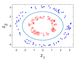
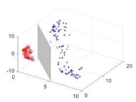
For the simulation, we recall the same setup in dsvm based on the example given in russell2010artificial . Consider ${N=200}$ uniformly distributed sample data points ${\boldsymbol{\chi}_{i}=[{\chi}_{i}(1);{\chi}_{i}(2)]}$ as shown in Fig. 2(Left), classified as blue *’s and red o’s. In $\mathbb{R}^{2}$, no linear SVM classifier can be defined, and applying nonlinear mapping $\phi(\boldsymbol{\chi}_{i})=[{\chi}_{i}(1)^{2};{\chi}_{i}(2)^{2};\sqrt{2}{\chi}_{i}(1){\chi}_{i}(2)]$ (with kernel $K(\boldsymbol{\chi}_{i},\boldsymbol{\chi}_{j})=(\phi(\boldsymbol{\chi}_{i})^{\top}\phi(\boldsymbol{\chi}_{j}))^{2}$) the data points can be linearly classified in $\mathbb{R}^{3}$ ($m=4$), see Fig. 2(Right).

Figure 2: (Left) This figure shows the training data and the optimal nonlinear classifier (Left) in 2D as the ellipse and (Right) (mapped) in 3D space as a linear hyperplane. Our nonlinear D-SVM under logarithmic quantization optimally classifies the data via the grey hyperplane. This hyperplane, inversely mapped back into 2D, represents the ellipse in the left figure.

For the purpose of the simulation, we assume nonlinear log quantization at the links in the proposed dynamics (16)-(17), i.e.,

$$g(z)=q_{l}(z)=\mbox{sgn}(z)\exp\left(\rho\left[\dfrac{\log(|z|)}{\rho}\right]\right)$$

with $[\cdot]$ as rounding to the nearest integer, $\mbox{sgn}(\cdot)$ as the sign function, and $\rho$ as the quantization level. This nonlinearity satisfies Assumption 2. The network $\mathcal{G}_{q}$ of ${n=5}$ agents is considered as a dynamic $2$-hop WB digraph such that, using MATLAB’s randperm, the nodes’ permutation (and neighbourhood) changes every $0.001$ sec. Every agent finds the optimal hyperplane parameters $\mathbf{x}_{i}=[\boldsymbol{\omega}_{i}^{\top};\nu_{i}]$ ($\boldsymbol{\omega}_{i}\in\mathbb{R}^{3}$) to minimize its local loss function defined by (5) and, then, shares $\mathbf{x}_{i}$ and $\mathbf{y}_{i}$ over $\mathcal{G}_{q}$. The simulation parameters are as follows: ${\alpha=6}$, $\mu=2$, $C=1$, $\rho=1$ with initialization $\mathbf{y}(0)=\mathbf{0}_{20}$ and $\mathbf{x}(0)=\texttt{rand(20,1)}$. The time-evolution of $\mathbf{x}_{i}=[\boldsymbol{\omega}_{i}^{\top};\nu_{i}]\in\mathbb{R}^{4}$, loss function $F(\mathbf{x})$, and sum of the gradients $\sum_{i=1}^{5}\nabla f_{i}(\mathbf{x}_{i})\in\mathbb{R}^{4}$ are given in Fig. 3.

Figure 3: The time-evolution of the parameters  ${\omega}_{i}$ and $\nu_{i}$ under the nonlinear D-SVM classifier dynamics (16)-(17) subject to log quantization. The overall loss function $F(\mathbf{x})$, the optimal values based on the centralized SVM, and the sum of the local gradients $\sum_{i=1}^{5}\nabla f_{i}(\mathbf{x}_{i})$ are also shown.

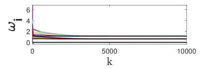
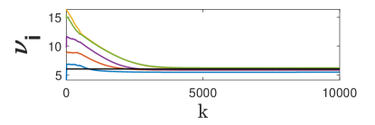
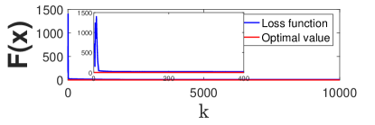
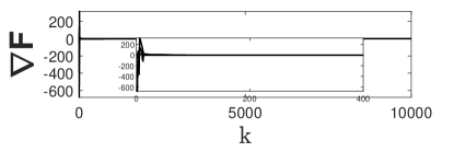
The agents reach consensus on the optimal value ${\overline{\mathbf{x}}^{*}=[\overline{\omega}(1),\overline{\omega}(2),\overline{\omega}(3),\overline{\nu}]^{\top}}$, which represents the separating ellipse ${\overline{\omega}(1)z_{1}^{2}+\overline{\omega}(2)z_{2}^{2}-\overline{\nu}=0}$ ($z_{1}$ and $z_{2}$ as the Cartesian coordinates in $\mathbb{R}^{2}$). For comparison, D-SVM under linear setup dsvm is also given in Fig. 4. It is clear that the nonlinearity only affects the agents’ dynamics and not the overall Laplacian-gradient tracking performance given by dynamics (35)-(36).

Figure 4: The time-evolution of the linear D-SVM classifier under dynamics (6)-(7) (under the same parameters as in Fig. 3) for comparison.

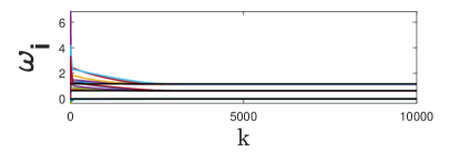
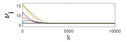
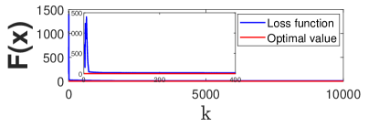
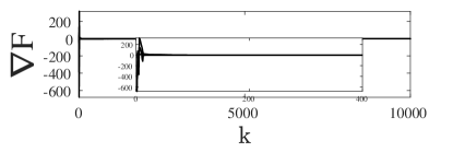
We used MATLAB R2021b for the simulation and CVX toolbox for centralized SVM (for comparison). As clear from the figures, the distributed solutions converge to the centralized optimal solution in both linear and quantized cases for admissible $\alpha,\rho$ values. Although, since the loss function (5) grows exponentially, this results in some inaccuracy in MATLAB calculations and minor residual in the figures.

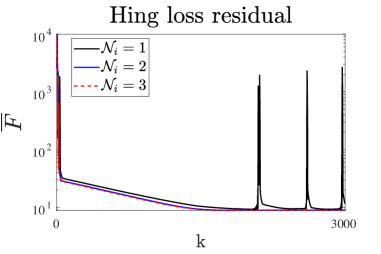
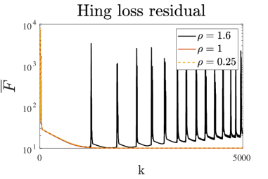
Next, we perform some sensitivity analysis on $\alpha_{g}$ by adding an extra link to reduce the network diameter to change $\sigma(M_{0}^{g})$ and, also, by changing the sector-bound-ratios by tuning the level $\rho$ in log quantization since $\kappa=1-\dfrac{\rho}{2}\leq\dfrac{q_{l}(z)}{z}\leq 1+\dfrac{\rho}{2}=\mathcal{K}$ (Assumption 2). We also tuned the network connectivity by changing the number of neighbours by linking the $2$-hop and $3$-hop neighbouring nodes. The results are shown in Fig. 5 for $\alpha=0.2$ and discrete time-step $\eta=0.05$. Note that, from the figure, large values of $\frac{\mathcal{K}}{\kappa}$ (Table 1) and $\frac{|\lambda_{2mn}|}{\underline{\lambda}}$ (Table 2) reduces the admissible range of $\alpha$ and makes the solution unstable for the given $\alpha$.

Figure 5: This figure shows how the change in network parameter $\mathcal{N}_{i}$ (and its eigen-spectrum) and the sector-bounds (the quantization parameter $\rho$) on the nonlinear mapping affect the stability of the dynamics (16)-(17).

Table 1: Change in the sector-bound-ratio by changing the log quantization level $\rho$

Sector-bound-ratio	$\rho=1.6$	$\rho=1$	$\rho=0.25$
$\frac{\mathcal{K}}{\kappa}$	9	3	1.28

Table 2: Change in the eigen-ratio by changing the network connectivity (number of $\mathcal{N}_{i}$-hop neighbours)

Eigen-ratio	$\mathcal{N}_{i}=1$	$\mathcal{N}_{i}=2$	$\mathcal{N}_{i}=3$
$\frac{\mbox{Max}\{|\lambda_{2mn}(t)|\}}{\underline{\lambda}}$	13733	2971	1413
$\frac{\mbox{Mean}\{|\lambda_{2mn}(t)|\}}{\underline{\lambda}}$	328	65	33

7 Discussions and Future Directions

7.1 Concluding Remarks

The consensus optimization algorithm in this work is shown to converge under strongly sign-preserving odd nonlinearities. Note that “non-strongly” sign-preserving nonlinearities may cause steady-state residuals as discussed in some recent works. For example, for general non-quadratic optimization subject to uniform quantization the existing methods only guarantee convergence to the $\varepsilon$-neighborhood of the exact optimizer $\mathbf{x}^{*}$, i.e., the algorithm may result in steady-state residual bounded by $\varepsilon$ magnusson2018communication . As an example consider uniform quantization defined as $g(z)=\rho\left[\dfrac{z}{\rho}\right]$. This nonlinear function although is sign-preserving, is not “strongly” sign-preserving as $\frac{g(z)}{z}=0$ for $-\frac{\rho}{2}<z<\frac{\rho}{2}$. This implies that in the proof of Theorem 2 the Eq. (59) does not necessarily hold (invariant set includes an $\varepsilon$-neighborhood of $\delta=\mathbf{0}$) and exact convergence is not guaranteed. Finding this $\varepsilon$ bound on the optimizer as a function of quantization level $\rho$ and loss function parameters is an interesting direction for future research. Recall that the logarithmic quantizer, on the other hand, is “strongly” sign-preserving and sector-bounded (satisfying Assumption 2). Thus, one can prove its convergence under (16)-(17) as shown in our simulations. Note that, although locally non-Lipschitz, log quantization satisfies Assumption 2 with no chattering effect (in contrast to rahili_ren ; ning2017distributed ; taes2020finite ). The results can be further extended to optimize the loss function (least mean-square-error problem) in distributed estimation doostmohammadian2021distributed ; my_acc and target tracking doostmohammadian2022linear .

7.2 Future Research

Generalizing Assumption 2 for less constrained link nonlinearity condition, extending Corollary 2 (and Assumption 3), and convergence under data-transmission delays over the links are our future research directions.

Statements & Declarations

The authors would like to thank Wei Jiang, Evagoras Makridis, Muwahida Liaquat, Themistoklis Charalambous, and Usman Khan for their comments.

The authors declare that no funds, grants, or other support were received during the preparation of this manuscript.

The authors have no relevant financial or non-financial (or other competing) interests to disclose.

All authors contributed to the study conception, preparation, and writing. All authors read and approved the final manuscript.

This research involves NO human or animal subjects.

Data sharing not applicable to this article as no datasets were generated or analysed during the current study.

References

- (1) Akbari, M., Gharesifard, B., Linder, T.: Distributed online convex optimization on time-varying directed graphs. IEEE Transactions on Control of Network Systems 4(3), 417–428 (2015)
- (2) Bhatia, R.: Perturbation bounds for matrix eigenvalues. SIAM (2007)
- (3) Cai, K., Ishii, H.: Average consensus on general strongly connected digraphs. Automatica 48(11), 2750–2761 (2012)
- (4) Chapelle, O.: Training a support vector machine in the primal. Neural computation 19(5), 1155–1178 (2007)
- (5) Chatterjee, S., Kalaimani, R.: Distributed optimization of average consensus containment with multiple stationary leaders. In: IEEE European Control Conference, pp. 1814–1819 (2022)
- (6) Cortes, C., Vapnik, V.: Support-vector networks. Machine learning 20, 273–297 (1995)
- (7) Doostmohammadian, M.: Single-bit consensus with finite-time convergence: Theory and applications. IEEE Transactions on Aerospace and Electronic Systems 56(4), 3332–3338 (2020)
- (8) Doostmohammadian, M., Aghasi, A., Charalambous, T., Khan, U.A.: Distributed support vector machines over dynamic balanced directed networks. IEEE Control Systems Letters 6, 758 – 763 (2021)
- (9) Doostmohammadian, M., Aghasi, A., Pirani, M., Nekouei, E., Khan, U.A., Charalambous, T.: Fast-convergent anytime-feasible dynamics for distributed allocation of resources over switching sparse networks with quantized communication links. In: IEEE European Control Conference, pp. 84–89 (2022)
- (10) Doostmohammadian, M., Aghasi, A., Vrakopoulou, M., Charalambous, T.: 1st-order dynamics on nonlinear agents for resource allocation over uniformly-connected networks. In: IEEE Conference on Control Technology and Applications (CCTA), pp. 1184–1189 (2022)
- (11) Doostmohammadian, M., Charalambous, T.: Linear tdoa-based measurements for distributed estimation and localized tracking. In: IEEE 95th Vehicular Technology Conference:(VTC2022-Spring), pp. 1–6. IEEE (2022)
- (12) Doostmohammadian, M., Khan, U.A.: Topology design in networked estimation: A generic approach. In: 2013 American Control Conference, pp. 4134–4139. IEEE (2013)
- (13) Doostmohammadian, M., Khan, U.A., Aghasi, A.: Distributed constraint-coupled optimization over unreliable networks. In: 10th IEEE/RSI International Conference on Robotics and Mechatronics (ICRoM), pp. 371–376. IEEE (2022)
- (14) Doostmohammadian, M., Pirani, M., Khan, U.A., Charalambous, T.: Consensus-based distributed estimation in the presence of heterogeneous, time-invariant delays. IEEE Control Systems Letters 6, 1598 – 1603 (2021)
- (15) Doostmohammadian, M., Taghieh, A., Zarrabi, H.: Distributed estimation approach for tracking a mobile target via formation of uavs. IEEE Transactions on Automation Science and Engineering 19(4), 3765–3776 (2021)
- (16) Drucker, H., Burges, C.J., Kaufman, L., Smola, A., Vapnik, V.: Support vector regression machines. Advances in neural information processing systems (NIPS) 9, 155–161 (1996)
- (17) Drummond, R., Duncan, S.: The aizerman and kalman conjectures using symmetry. Automatica 92, 240–243 (2018)
- (18) Fagnani, F., Zampieri, S.: Average consensus with packet drop communication. SIAM Journal on Control and Optimization 48(1), 102–133 (2009). DOI 10.1137/060676866
- (19) Forero, P.A., Cano, A., Giannakis, G.B.: Consensus-based distributed support vector machines. Journal of Machine Learning Research 11(5) (2010)
- (20) Garg, K., Baranwal, M., Hero, A.O., Panagou, D.: Fixed-time distributed optimization under time-varying communication topology. arXiv preprint arXiv:1905.10472 (2019)
- (21) Gharesifard, B., Cortés, J.: Distributed continuous-time convex optimization on weight-balanced digraphs. IEEE Transactions on Automatic Control 59(3), 781–786 (2014)
- (22) Goebel, R., Sanfelice, R., Teel, A.: Hybrid dynamical systems. IEEE control systems magazine 29(2), 28–93 (2009)
- (23) Jahvani, M., Guay, M.: Distributed convex optimization on the nonnegative orthant. In: IEEE European Control Conference, pp. 1955–1959 (2022)
- (24) Jiang, W., Doostmohammadian, M., Charalambous, T.: Distributed resource allocation via ADMM over digraphs. In: 61st IEEE Conference on Decision and Control, pp. 5645–5651. IEEE (2022)
- (25) Jurafsky, D., Martin, J.H.: Speech and Language Processing. Prentice Hall (2020)
- (26) Koppel, A., Paternain, S., Richard, C., Ribeiro, A.: Decentralized online learning with kernels. IEEE Transactions on Signal Processing 66(12), 3240–3255 (2018)
- (27) Ling, Q., Ribeiro, A.: Decentralized dynamic optimization through the alternating direction method of multipliers. IEEE Transactions on Signal Processing 62(5), 1185–1197 (2013)
- (28) Liu, Y.Y., Slotine, J.J., Barabási, A.L.: Controllability of complex networks. Nature 473(7346), 167–173 (2011). DOI 10.1038/nature10011
- (29) Liu, Z., Stursberg, O.: Distributed optimization for mixed-integer consensus in multi-agent networks. In: IEEE European Control Conference, pp. 2157–2163 (2022)
- (30) Magnússon, S., Enyioha, C., Li, N., Fischione, C., Tarokh, V.: Communication complexity of dual decomposition methods for distributed resource allocation optimization. IEEE Journal of Selected Topics in Signal Processing 12(4), 717–732 (2018)
- (31) Navia-Vázquez, A., Gutierrez-Gonzalez, D., Parrado-Hernández, E., Navarro-Abellan, J.J.: Distributed support vector machines. IEEE Transactions on Neural Networks 17(4), 1091 (2006)
- (32) Nedic, A., Olshevsky, A., Shi, W.: Achieving geometric convergence for distributed optimization over time-varying graphs. SIAM Journal on Optimization 27(4), 2597–2633 (2017)
- (33) Ning, B., Han, Q., Zuo, Z.: Distributed optimization for multiagent systems: An edge-based fixed-time consensus approach. IEEE Transactions on Cybernetics 49(1), 122–132 (2017)
- (34) Olfati-Saber, R., Murray, R.M.: Consensus problems in networks of agents with switching topology and time-delays. IEEE Transactions on Automatic Control 49, no. 9, 1520–1533 (2004)
- (35) Rahili, S., Ren, W.: Distributed continuous-time convex optimization with time-varying cost functions. IEEE Transactions on Automatic Control 62(4), 1590–1605 (2017). DOI 10.1109/TAC.2016.2593899
- (36) Russell, S., Norvig, P.: Artificial intelligence: a modern approach (2010)
- (37) Safavi, S., Khan, U.A.: Asymptotic stability of stochastic ltv systems with applications to distributed dynamic fusion. IEEE Trans. on Automatic Control 62(11), 5888–5893 (2017)
- (38) Simonetto, A., Koppel, A., Mokhtari, A., Leus, G., Ribeiro, A.: Decentralized prediction-correction methods for networked time-varying convex optimization. IEEE Transactions on Automatic Control 62(11), 5724–5738 (2017)
- (39) Slotine, J., Li, W.: Applied nonlinear control. Prentice-Hall (1991)
- (40) Stanković, S.S., Beko, M., Stanković, M.S.: Nonlinear robustified stochastic consensus seeking. Systems & Control Letters 139, 104667 (2020)
- (41) Stewart, G.W., Sun, J.: Matrix perturbation theory. Academic Press (1990)
- (42) Toghani, M., Uribe, C.A.: On arbitrary compression for decentralized consensus and stochastic optimization over directed networks. In: IEEE European Control Conference, pp. 72–77 (2022)
- (43) Vaidya, N.H., Hadjicostis, C.N., Dominguez-Garcia, A.D.: Robust average consensus over packet dropping links: Analysis via coefficients of ergodicity. In: 51st IEEE Conference on Decision and Control, pp. 2761–2766 (2012). DOI 10.1109/CDC.2012.6426252
- (44) Van Scoy, B., Lessard, L.: A distributed optimization algorithm over time-varying graphs with efficient gradient evaluations. IFAC-PapersOnLine 52(20), 357–362 (2019)
- (45) Xi, C., Xin, R., Khan, U.A.: ADD-OPT: Accelerated distributed directed optimization. IEEE Transactions on Automatic Control 63(5), 1329–1339 (2017)