SALSA: A Sequential Alternating Least Squares Approximation Method For MIMO Channel Estimation

Sepideh Gherekhloo, Khaled Ardah, Martin Haardt S. Gherekhloo and M. Haardt are with the Communications Research Laboratory (CRL), TU Ilmenau, Ilmenau, Germany (e-mail: {sepideh.gherekhloo, martin.haardt}@tu-ilmenau.de). K. Ardah is with Lenovo (Deutschland) GmbH (e-mail: kardah@lenovo.com).
Abstract

In this paper, we consider the channel estimation problem in sub-6 GHz uplink wideband MIMO-OFDM communication systems, where a user equipment with a fully-digital beamforming structure is communicating with a base station having a hybrid analog-digital beamforming structure. A novel channel estimation method called Sequential Alternating Least Squares Approximation (SALSA) is proposed by exploiting a hidden tensor structure in the uplink measurement matrix. Specifically, by showing that any MIMO channel matrix can be approximately decomposed into a summation of R𝑅R factor matrices having a Kronecker structure, the uplink measurement matrix can be reshaped into a 3-way tensor admitting a Tucker decomposition. Exploiting the tensor structure, the MIMO channel matrix is estimated sequentially using an alternating least squares method. Detailed simulation results are provided showing the effectiveness of the proposed SALSA method as compared to the classical least squares method.

Index Terms:
Channel estimation, massive MIMO, Tucker tensor decomposition, alternating least squares

I Introduction

Massive MIMO [1] is one of the key enabling technologies of 5G-NR mobile communications [2] and it shall remain relevant in future 6G wireless systems. By employing a large number of antennas at the base station (BS) relative to the number of scheduled users, massive MIMO systems increase the data throughput relative to legacy systems by providing a large beamforming gain and an improved multi-user interference suppression owing to its high spatial resolution [3]. Recently, massive MIMO communications have received a special attention with the introduction of millimeter-wave (mm-wave)-based wireless communications [4], since the use of massive MIMO in such systems becomes a requirement rather than an option to compensate the high pathloss encountered in the wireless communication systems at higher frequencies. However, it is well-known that the promised theoretical massive MIMO gains heavily rely on the availability of accurate channel state information (CSI) and the considered beamforming structure.

On the one hand, classical fully-digital (FD) beamforming structures, which generally provide the maximum beamforming gain, require a dedicated radio frequency (RF) chain for each antenna element. This increases not only the implementation cost and complexity of massive MIMO systems, but also the circuit energy consumption. A promising solution to these issues relies on the recently introduced hybrid analog-digital (HAD) beamforming structures [5, 6, 4, 7, 8], which use a combination of analog beamforming in the RF domain and digital beamforming in the baseband domain to reduce the number of RF chains as compared to FD beamforming structures, e.g., the number of RF chains can be as small as the number of transmitted data streams.

On the other hand, in 5G-NR systems, for example, the BS estimates the CSI from uplink sounding reference signals (SRS) emitted by the user terminals (UEs). In mm-wave systems, the CSI estimation problem is often transformed into a multi-dimensional direction-of-arrival (DoA) estimation problem [9, 10, 11], thanks to the low-rank (sparse) nature of mm-wave MIMO channels [4], where several techniques, e.g., compressed sensing [9, 10] and ESPRIT [11] can be readily employed to obtain a high CSI estimation accuracy while requiring a small number of training overhead. Differently, in sub-6 GHz-based systems, the MIMO channels often experience a high-rank nature, which makes most, if not all, mm-wave-based MIMO channel estimation methods unfeasible. To this end, classical channel estimation techniques, e.g., least-squares (LS) and minimum mean squared-error (MMSE) methods [12, 13] can be used to estimate sub-6 GHz-based MIMO channels. However, these methods were originally developed for single-antenna and small-scale MIMO systems and suffer from a severe performance degradation in difficult scenarios, e.g., with small number of training snapshots and/or a low signal-to-noise ratio (SNR). Since sub-6 GHz massive MIMO communications are, and will remain, an integral part of current and future wireless communication systems, more efficient channel estimation techniques than the classical methods are required.

In this paper, we consider the channel estimation problem in sub-6 GHz uplink wideband MIMO-OFDM communication systems, where a single-user with a FD beamforming structure communicates with a BS having a HAD beamforming structure. By exploiting a hidden tensor structure in the uplink measurement matrix, we propose a novel channel estimation method called Sequential Alternating Least Squares Approximation (SALSA). Specifically, by showing that any MIMO channel matrix can be approximately decomposed into a summation of R𝑅R factor matrices having a Kronecker structure, the uplink measurement matrix can be reshaped into a 3-way tensor admitting a Tucker decomposition [14]. Exploiting such a tensor representation, the MIMO channel matrix can be estimated sequentially using the classical ALS method [15]. Detailed simulation results are provided showing that the SALSA-based approach can achieve a more accurate channel estimation in difficult scenarios as compared to the classical LS-based approach.

Notation: The transpose, the complex conjugate, the conjugate transpose (Hermitian), and the Kronecker product are denoted as 𝑨𝖳superscript𝑨𝖳{\bm{A}}^{\mathsf{T}}, 𝑨superscript𝑨{\bm{A}}^{*}, 𝑨𝖧superscript𝑨𝖧{\bm{A}}^{\mathsf{H}}, and tensor-product\otimes, respectively. Moreover, 𝑰Nsubscript𝑰𝑁{\bm{I}}_{N} is the N×N𝑁𝑁N\times N identity matrix, vec{𝑨}vec𝑨\text{vec}\{{\bm{A}}\} forms a vector by staking the columns of 𝑨𝑨{\bm{A}} over each other, and the n𝑛n-mode product of a tensor 𝓐I1×I2×,×IN𝓐superscriptsubscript𝐼1subscript𝐼2absentsubscript𝐼𝑁\bm{\mathcal{A}}\in\mathbb{C}^{I_{1}\times I_{2}\times\dots,\times I_{N}} with a matrix 𝑩J×In𝑩superscript𝐽subscript𝐼𝑛{\bm{B}}\in\mathbb{C}^{J\times I_{n}} is denoted as 𝓐×n𝑩subscript𝑛𝓐𝑩\bm{\mathcal{A}}\times_{n}{\bm{B}}.

II System Model

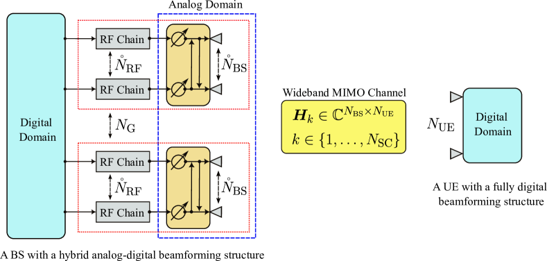
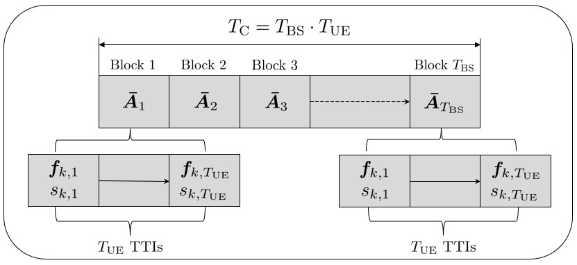
We consider an uplink single-user wideband MIMO-OFDM communication system, as depicted in Fig. 1, where a UE with NUEsubscript𝑁UEN_{\text{UE}} antennas is communicating with a BS with NBSsubscript𝑁BSN_{\text{BS}} antennas over NSCsubscript𝑁SCN_{\text{SC}} subcarriers. The UE has a FD beamforming structure while the BS has a HAD beamforming structure with NRFNBSsubscript𝑁RFsubscript𝑁BSN_{\text{RF}}\leq N_{\text{BS}} radio-frequency (RF) chains. We assume that the NBSsubscript𝑁BSN_{\text{BS}} antennas and the NRFsubscript𝑁RFN_{\text{RF}} RF chains are divided equally111To simplify the exposition, we assume that NBSsubscript𝑁BSN_{\text{BS}}, NRFsubscript𝑁RFN_{\text{RF}}, and NGsubscript𝑁GN_{\text{G}} are selected so that N̊BSsubscript̊𝑁BS\mathring{N}_{\text{BS}} and N̊RFsubscript̊𝑁RF\mathring{N}_{\text{RF}} are integer numbers, without loss of generality. into NG1subscript𝑁G1N_{\text{G}}\geq 1 groups, where each group has N̊BS=NBSNGsubscript̊𝑁BSsubscript𝑁BSsubscript𝑁G\mathring{N}_{\text{BS}}=\frac{N_{\text{BS}}}{N_{\text{G}}} antennas and N̊RF=NRFNGsubscript̊𝑁RFsubscript𝑁RFsubscript𝑁G\mathring{N}_{\text{RF}}=\frac{N_{\text{RF}}}{N_{\text{G}}} RF chains (i.e., NBS=NGN̊BSsubscript𝑁BSsubscript𝑁Gsubscript̊𝑁BSN_{\text{BS}}=N_{\text{G}}\cdot\mathring{N}_{\text{BS}} and NRF=NGN̊RFsubscript𝑁RFsubscript𝑁Gsubscript̊𝑁RFN_{\text{RF}}=N_{\text{G}}\cdot\mathring{N}_{\text{RF}}) and the RF chains in every group are connected with every antenna element in the same group. Moreover, we assume a block-fading channel model as shown in Fig. 2, where the channel coherence-time TCsubscript𝑇CT_{\text{C}} is divided into TBSTUEsubscript𝑇BSsubscript𝑇UET_{\text{BS}}T_{\text{UE}} transmission time intervals (TTIs), i.e., every block has TUEsubscript𝑇UET_{\text{UE}} snapshots.

Let 𝑨¯iNBS×NRFsubscriptbold-¯𝑨𝑖superscriptsubscript𝑁BSsubscript𝑁RF\bm{\bar{A}}_{i}\in\mathbb{C}^{N_{\text{BS}}\times N_{\text{RF}}} denote the analog combining matrix at the i𝑖ith block at the BS. Then, according to our above assumptions, 𝑨¯isubscriptbold-¯𝑨𝑖\bm{\bar{A}}_{i} has a block-diagonal structure given as222Note that if NG=1subscript𝑁G1N_{\text{G}}=1, the above analog structure coincides with the known fully-connected analog structure [5], where every RF chain is connected to every antenna element. On the other hand, if NG=NRFsubscript𝑁Gsubscript𝑁RFN_{\text{G}}=N_{\text{RF}}, the above analog structure coincides with the known partially-connected analog structure [5], where every RF chain is connected to a unique subset of antenna elements.

𝑨¯i=1N̊BS[𝑨¯i,1𝟎𝟎𝑨¯i,NG]NBS×NRF,subscriptbold-¯𝑨𝑖1subscript̊𝑁BSmatrixsubscriptbold-¯𝑨𝑖100subscriptbold-¯𝑨𝑖subscript𝑁Gsuperscriptsubscript𝑁BSsubscript𝑁RF\displaystyle\bm{\bar{A}}_{i}=\frac{1}{\sqrt{\mathring{N}_{\text{BS}}}}\cdot\begin{bmatrix}\bm{\bar{A}}_{i,1}&\dots&{\bm{0}}\\ \vdots&\ddots&\vdots\\ {\bm{0}}&\dots&\bm{\bar{A}}_{i,N_{\text{G}}}\end{bmatrix}\in\mathbb{C}^{N_{\text{BS}}\times N_{\text{RF}}}, (1)

where 𝑨¯i,gN̊BS×N̊RFsubscriptbold-¯𝑨𝑖𝑔superscriptsubscript̊𝑁BSsubscript̊𝑁RF\bm{\bar{A}}_{i,g}\in\mathbb{C}^{\mathring{N}_{\text{BS}}\times\mathring{N}_{\text{RF}}} is the g𝑔gth block-matrix with constant modulus entries, i.e., |[𝑨¯i,g][r,c]|=1subscriptdelimited-[]subscriptbold-¯𝑨𝑖𝑔𝑟𝑐1\big{|}[\bm{\bar{A}}_{i,g}]_{[r,c]}\big{|}=1, where [𝑨¯i,g][r,c]subscriptdelimited-[]subscriptbold-¯𝑨𝑖𝑔𝑟𝑐[\bm{\bar{A}}_{i,g}]_{[r,c]} is the (r,c)𝑟𝑐(r,c)th entry of 𝑨¯i,gsubscriptbold-¯𝑨𝑖𝑔\bm{\bar{A}}_{i,g}.

The received signal by the BS in the (i,j)𝑖𝑗(i,j)th TTI over the k𝑘kth subcarrier, with i{1,,TBS}𝑖1subscript𝑇BSi\in\{1,\dots,T_{\text{BS}}\}, j{1,,TUE}𝑗1subscript𝑇UEj\in\{1,\dots,T_{\text{UE}}\}, k{1,,NSC}𝑘1subscript𝑁SCk\in\{1,\dots,N_{\text{SC}}\}, can be expressed as

𝒚¯k,i,j=𝑨¯i𝖧𝑯k𝒇k,jsk,j+𝑨¯i𝖧𝒛¯k,i,jNRF,subscriptbold-¯𝒚𝑘𝑖𝑗subscriptsuperscriptbold-¯𝑨𝖧𝑖subscript𝑯𝑘subscript𝒇𝑘𝑗subscript𝑠𝑘𝑗subscriptsuperscriptbold-¯𝑨𝖧𝑖subscriptbold-¯𝒛𝑘𝑖𝑗superscriptsubscript𝑁RF\displaystyle\bm{\bar{y}}_{k,i,j}=\bm{\bar{A}}^{\mathsf{H}}_{i}{\bm{H}}_{k}{\bm{f}}_{k,j}s_{k,j}+\bm{\bar{A}}^{\mathsf{H}}_{i}\bm{\bar{z}}_{k,i,j}\in\mathbb{C}^{N_{\text{RF}}}, (2)

where 𝒇k,jNUEsubscript𝒇𝑘𝑗superscriptsubscript𝑁UE{\bm{f}}_{k,j}\in\mathbb{C}^{{N}_{\text{UE}}} is the (k,j)𝑘𝑗(k,j)th precoding vector, sk,jsubscript𝑠𝑘𝑗s_{k,j}\in\mathbb{C} is the corresponding training symbol, 𝒛¯i,jNBSsubscriptbold-¯𝒛𝑖𝑗superscriptsubscript𝑁BS\bm{\bar{z}}_{i,j}\in\mathbb{C}^{{N}_{\text{BS}}} is the BS additive white Gaussian noise with zero mean and variance σn2superscriptsubscript𝜎𝑛2\sigma_{n}^{2}, and 𝑯kNBS×NUEsubscript𝑯𝑘superscriptsubscript𝑁BSsubscript𝑁UE{\bm{H}}_{k}\in\mathbb{C}^{{N}_{\text{BS}}\times{N}_{\text{UE}}} is the k𝑘kth subcarrier frequency-domain MIMO channel matrix.

Initially, we collect the measurement vectors {𝒚¯k,i,j}j=1TUEsuperscriptsubscriptsubscriptbold-¯𝒚𝑘𝑖𝑗𝑗1subscript𝑇UE\{\bm{\bar{y}}_{k,i,j}\}_{j=1}^{T_{\text{UE}}} next to each other as 𝒀¯k,i=[𝒚¯k,i,1,,𝒚¯k,i,TUE]subscriptbold-¯𝒀𝑘𝑖subscriptbold-¯𝒚𝑘𝑖1subscriptbold-¯𝒚𝑘𝑖subscript𝑇UE\bm{\bar{Y}}_{k,i}=[\bm{\bar{y}}_{k,i,1},\dots,\bm{\bar{y}}_{k,i,T_{\text{UE}}}], which can be written as

𝒀¯k,i=𝑨¯i𝖧𝑯k𝑭k+𝑨¯i𝖧𝒁¯k,iNRF×TUE,subscriptbold-¯𝒀𝑘𝑖subscriptsuperscriptbold-¯𝑨𝖧𝑖subscript𝑯𝑘subscript𝑭𝑘subscriptsuperscriptbold-¯𝑨𝖧𝑖subscriptbold-¯𝒁𝑘𝑖superscriptsubscript𝑁RFsubscript𝑇UE\displaystyle\bm{\bar{Y}}_{k,i}=\bm{\bar{A}}^{\mathsf{H}}_{i}{\bm{H}}_{k}{\bm{F}}_{k}+\bm{\bar{A}}^{\mathsf{H}}_{i}\bm{\bar{Z}}_{k,i}\in\mathbb{C}^{{N}_{\text{RF}}\times T_{\text{UE}}}, (3)

where 𝑭k=[𝒇k,1sk,1,,𝒇k,TUEsk,TUE]NUE×TUEsubscript𝑭𝑘subscript𝒇𝑘1subscript𝑠𝑘1subscript𝒇𝑘subscript𝑇UEsubscript𝑠𝑘subscript𝑇UEsuperscriptsubscript𝑁UEsubscript𝑇UE{\bm{F}}_{k}=[{\bm{f}}_{k,1}s_{k,1},\dots,{\bm{f}}_{k,T_{\text{UE}}}s_{k,T_{\text{UE}}}]\in\mathbb{C}^{{N}_{\text{UE}}\times T_{\text{UE}}} and 𝒁¯k,i=[𝒛¯k,i,1,,𝒛¯k,i,TUE]subscriptbold-¯𝒁𝑘𝑖subscriptbold-¯𝒛𝑘𝑖1subscriptbold-¯𝒛𝑘𝑖subscript𝑇UE\bm{\bar{Z}}_{k,i}=[\bm{\bar{z}}_{k,i,1},\dots,\bm{\bar{z}}_{k,i,T_{\text{UE}}}]. We assume that 𝑭k,ksubscript𝑭𝑘for-all𝑘{\bm{F}}_{k},\forall k, are designed with orthonormal rows, i.e., 𝑭k𝑭k𝖧=𝑰NUE,ksubscript𝑭𝑘subscriptsuperscript𝑭𝖧𝑘subscript𝑰subscript𝑁UEfor-all𝑘{\bm{F}}_{k}{\bm{F}}^{\mathsf{H}}_{k}={\bm{I}}_{N_{\text{UE}}},\forall k, and TUENUEsubscript𝑇UEsubscript𝑁UET_{\text{UE}}\geq N_{\text{UE}}. After applying the right-filtering to (3) we obtain

𝒀k,i=𝒀¯k,i𝑭𝖧=𝑨¯i𝖧𝑯k+𝒁k,iNRF×NUE,subscript𝒀𝑘𝑖subscriptbold-¯𝒀𝑘𝑖superscript𝑭𝖧subscriptsuperscriptbold-¯𝑨𝖧𝑖subscript𝑯𝑘subscript𝒁𝑘𝑖superscriptsubscript𝑁RFsubscript𝑁UE\displaystyle{\bm{Y}}_{k,i}=\bm{\bar{Y}}_{k,i}{\bm{F}}^{\mathsf{H}}=\bm{\bar{A}}^{\mathsf{H}}_{i}{\bm{H}}_{k}+{\bm{Z}}_{k,i}\in\mathbb{C}^{N_{\text{RF}}\times N_{\text{UE}}}, (4)

where 𝒁k,i=𝑨¯i𝖧𝒁¯k,i𝑭k𝖧subscript𝒁𝑘𝑖subscriptsuperscriptbold-¯𝑨𝖧𝑖subscriptbold-¯𝒁𝑘𝑖subscriptsuperscript𝑭𝖧𝑘{\bm{Z}}_{k,i}=\bm{\bar{A}}^{\mathsf{H}}_{i}\bm{\bar{Z}}_{k,i}{\bm{F}}^{\mathsf{H}}_{k}. Next, we collect the measurement matrices {𝒀k,i}i=1TBSsuperscriptsubscriptsubscript𝒀𝑘𝑖𝑖1subscript𝑇BS\{{\bm{Y}}_{k,i}\}_{i=1}^{T_{\text{BS}}} on the top of each other as 𝒀k=[𝒀k,1𝖳,,𝒀k,TBS𝖳]𝖳subscript𝒀𝑘superscriptsubscriptsuperscript𝒀𝖳𝑘1subscriptsuperscript𝒀𝖳𝑘subscript𝑇BS𝖳{\bm{Y}}_{k}=\big{[}{\bm{Y}}^{\mathsf{T}}_{k,1},\dots,{\bm{Y}}^{\mathsf{T}}_{k,T_{\text{BS}}}\big{]}^{\mathsf{T}}, which can be written as

𝒀k=𝑨𝑯k+𝒁kL×NUE,subscript𝒀𝑘𝑨subscript𝑯𝑘subscript𝒁𝑘superscript𝐿subscript𝑁UE\displaystyle{\bm{Y}}_{k}={\bm{A}}{\bm{H}}_{k}+{\bm{Z}}_{k}\in\mathbb{C}^{L\times N_{\text{UE}}}, (5)

where L=TBSNRF𝐿subscript𝑇BSsubscript𝑁RFL=T_{\text{BS}}{N}_{\text{RF}}, 𝑨=[𝑨¯1,,𝑨¯TBS]𝖧L×NBS𝑨superscriptsubscriptbold-¯𝑨1subscriptbold-¯𝑨subscript𝑇BS𝖧superscript𝐿subscript𝑁BS{\bm{A}}=\big{[}\bm{\bar{A}}_{1},\dots,\bm{\bar{A}}_{T_{\text{BS}}}\big{]}^{\mathsf{H}}\in\mathbb{C}^{L\times N_{\text{BS}}}, and 𝒁k=[𝒁k,1𝖳,,𝒁k,TBS𝖳]𝖳subscript𝒁𝑘superscriptsubscriptsuperscript𝒁𝖳𝑘1subscriptsuperscript𝒁𝖳𝑘subscript𝑇BS𝖳{\bm{Z}}_{k}=\big{[}{\bm{Z}}^{\mathsf{T}}_{k,1},\dots,{\bm{Z}}^{\mathsf{T}}_{k,T_{\text{BS}}}\big{]}^{\mathsf{T}}. After that, we collect the measurement matrices {𝒀k}k=1NSCsuperscriptsubscriptsubscript𝒀𝑘𝑘1subscript𝑁SC\{{\bm{Y}}_{k}\}_{k=1}^{N_{\text{SC}}} next to each other as 𝒀=[𝒀1,,𝒀NSC]𝒀subscript𝒀1subscript𝒀subscript𝑁SC\bm{{Y}}=[{\bm{Y}}_{1},\dots,{\bm{Y}}_{N_{\text{SC}}}], which can be written as

𝒀=𝑨𝑯+𝒁L×NUENSC,𝒀𝑨𝑯𝒁superscript𝐿subscript𝑁UEsubscript𝑁SC\displaystyle{\bm{Y}}={\bm{A}}{\bm{H}}+{\bm{Z}}\in\mathbb{C}^{L\times N_{\text{UE}}N_{\text{SC}}}, (6)

where 𝒁=[𝒁1,,𝒁NSC]𝒁subscript𝒁1subscript𝒁subscript𝑁SC{\bm{Z}}=\big{[}{\bm{Z}}_{1},\dots,{\bm{Z}}_{N_{\text{SC}}}\big{]} and 𝑯=[𝑯1,,𝑯NSC]NBS×NUENSC𝑯subscript𝑯1subscript𝑯subscript𝑁SCsuperscriptsubscript𝑁BSsubscript𝑁UEsubscript𝑁SC{\bm{H}}=\big{[}\bm{H}_{1},\dots,\bm{H}_{N_{\text{SC}}}\big{]}\in\mathbb{C}^{N_{\text{BS}}\times N_{\text{UE}}N_{\text{SC}}} is the total MIMO channel matrix.

Refer to caption
Figure 1: The considered uplink MIMO-OFDM communication system.
Refer to caption
Figure 2: The channel coherence time TCsubscript𝑇CT_{\text{C}} division.

The baseline LS-based channel estimation method: Given the measurement matrix in (6), a least-squares (LS)-based method can be used to obtain an estimate of the total MIMO channel matrix as

𝑯^LS=[𝑨]+𝒀=[𝑯^1,,𝑯^NSC]NBS×NUENSC,subscriptbold-^𝑯LSsuperscriptdelimited-[]𝑨𝒀subscriptbold-^𝑯1subscriptbold-^𝑯subscript𝑁SCsuperscriptsubscript𝑁BSsubscript𝑁UEsubscript𝑁SC\displaystyle\bm{\hat{H}}_{\text{LS}}=[{\bm{A}}]^{+}{\bm{Y}}=\big{[}\bm{\hat{H}}_{1},\dots,\bm{\hat{H}}_{N_{\text{SC}}}\big{]}\in\mathbb{C}^{N_{\text{BS}}\times N_{\text{UE}}N_{\text{SC}}}, (7)

where []+superscriptdelimited-[][\cdot]^{+} denotes the Moore-Penrose pseudo-inverse. Note that, due to the left filtering, the LS-based method requires that LNBS𝐿subscript𝑁BSL\geq N_{\text{BS}}, i.e., TBSNBSNRFsubscript𝑇BSsubscript𝑁BSsubscript𝑁RFT_{\text{BS}}\geq\frac{N_{\text{BS}}}{N_{\text{RF}}} to provide an accurate channel estimate.

III The proposed SALSA method

To obtain a more accurate channel estimate while reducing the training overhead, we propose in this section a novel channel estimation method called SALSA, which is derived by exploiting a hidden tensor structure in the measurement matrix in (6). To show this, we first recall the following propositions from [16, 17, 18].

Proposition 1: Let 𝑿𝑿{\bm{X}} be a matrix given as

𝑿=𝑿1𝑿2=[𝑿1,1𝑿1,J1𝑿I1,1𝑿I1,J1]I×J,𝑿tensor-productsubscript𝑿1subscript𝑿2matrixsubscript𝑿11subscript𝑿1subscript𝐽1subscript𝑿subscript𝐼11subscript𝑿subscript𝐼1subscript𝐽1superscript𝐼𝐽\displaystyle{\bm{X}}={\bm{X}}_{1}\otimes{\bm{X}}_{2}=\begin{bmatrix}{\bm{X}}_{1,1}&\dots&{\bm{X}}_{1,J_{1}}\\ \dots\\ {\bm{X}}_{I_{1},1}&\dots&{\bm{X}}_{I_{1},J_{1}}\\ \end{bmatrix}\in\mathbb{C}^{I\times J}, (8)

where 𝑿1I1×J1subscript𝑿1superscriptsubscript𝐼1subscript𝐽1{\bm{X}}_{1}\in\mathbb{C}^{I_{1}\times J_{1}}, 𝑿2I2×J2subscript𝑿2superscriptsubscript𝐼2subscript𝐽2{\bm{X}}_{2}\in\mathbb{C}^{I_{2}\times J_{2}}, I=I1I2𝐼subscript𝐼1subscript𝐼2I=I_{1}I_{2}, J=J1J2𝐽subscript𝐽1subscript𝐽2J=J_{1}J_{2}, and 𝑿n,m=[𝑿1][n,m]𝑿2subscript𝑿𝑛𝑚subscriptdelimited-[]subscript𝑿1𝑛𝑚subscript𝑿2{\bm{X}}_{n,m}=[{\bm{X}}_{1}]_{[n,m]}{\bm{X}}_{2} is the (n,m)𝑛𝑚(n,m)th block-matrix of 𝑿𝑿{\bm{X}}. Let 𝑲I1J1×I2J2𝑲superscriptsubscript𝐼1subscript𝐽1subscript𝐼2subscript𝐽2{\bm{K}}\in\mathbb{C}^{I_{1}J_{1}\times I_{2}J_{2}} be a rank-one matrix given as

𝑲=[vec{𝑿1,1}Tvec{𝑿I1,1}Tvec{𝑿1,J1}Tvec{𝑿I1,J1}T]=vec{𝑿1}vec{𝑿2}T,𝑲matrixvecsuperscriptsubscript𝑿11Tvecsuperscriptsubscript𝑿subscript𝐼11Tvecsuperscriptsubscript𝑿1subscript𝐽1Tvecsuperscriptsubscript𝑿subscript𝐼1subscript𝐽1Tvecsubscript𝑿1vecsuperscriptsubscript𝑿2T\displaystyle{\bm{K}}=\begin{bmatrix}\text{vec}\{{\bm{X}}_{1,1}\}^{\text{T}}\\ \dots\\ \text{vec}\{{\bm{X}}_{I_{1},1}\}^{\text{T}}\\ \dots\\ \text{vec}\{{\bm{X}}_{1,J_{1}}\}^{\text{T}}\\ \dots\\ \text{vec}\{{\bm{X}}_{I_{1},J_{1}}\}^{\text{T}}\\ \end{bmatrix}=\text{vec}\{{\bm{X}}_{1}\}\text{vec}\{{\bm{X}}_{2}\}^{\text{T}}, (9)

with the rank-one truncated-SVD given as 𝑲=σ𝒖𝒗H𝑲𝜎𝒖superscript𝒗H{\bm{K}}=\sigma{\bm{u}}{\bm{v}}^{\text{H}}, where 𝒖I1J1𝒖superscriptsubscript𝐼1subscript𝐽1{\bm{u}}\in\mathbb{C}^{I_{1}J_{1}} and 𝒗I2J2𝒗superscriptsubscript𝐼2subscript𝐽2{\bm{v}}\in\mathbb{C}^{I_{2}J_{2}} are the left and right singular vectors of 𝑲𝑲{\bm{K}}, respectively, and σ𝜎\sigma is the associated singular value. Then, the optimal solution to

minimize 𝑿1,𝑿2𝑿(𝑿1𝑿2)F2subscript𝑿1subscript𝑿2minimize subscriptsuperscriptnorm𝑿tensor-productsubscript𝑿1subscript𝑿22F\displaystyle\underset{{\bm{X}}_{1},{\bm{X}}_{2}}{\text{minimize }}\|{\bm{X}}-\big{(}{\bm{X}}_{1}\otimes{\bm{X}}_{2}\big{)}\|^{2}_{\text{F}} (10)

can be obtained as

𝑿1subscript𝑿1\displaystyle{\bm{X}}_{1} =reshape{σ𝒖,I1,J1}absentreshape𝜎𝒖subscript𝐼1subscript𝐽1\displaystyle=\text{reshape}\{\sqrt{\sigma}{\bm{u}},I_{1},J_{1}\} (11)
𝑿2subscript𝑿2\displaystyle{\bm{X}}_{2} =reshape{σ𝒗,I2,J2}.absentreshape𝜎superscript𝒗subscript𝐼2subscript𝐽2\displaystyle=\text{reshape}\{\sqrt{\sigma}{\bm{v}}^{*},I_{2},J_{2}\}. (12)

Proof: Please refer to [17] for more details.

Proposition 2: For any given I×J𝐼𝐽I\times J matrix 𝑿𝑿{\bm{X}}, it can be approximately written as a summation of R1𝑅1R\geq 1 factor matrices as

𝑿=r=1R𝑿r=r=1R𝑿1,r𝑿2,r,𝑿superscriptsubscript𝑟1𝑅subscript𝑿𝑟superscriptsubscript𝑟1𝑅tensor-productsubscript𝑿1𝑟subscript𝑿2𝑟\displaystyle{\bm{X}}=\sum_{r=1}^{R}{\bm{X}}_{r}=\sum_{r=1}^{R}{\bm{X}}_{1,r}\otimes{\bm{X}}_{2,r}, (13)

where 𝑿r=𝑿1,r𝑿2,rsubscript𝑿𝑟tensor-productsubscript𝑿1𝑟subscript𝑿2𝑟{\bm{X}}_{r}={\bm{X}}_{1,r}\otimes{\bm{X}}_{2,r}, 𝑿1,rI1×J1subscript𝑿1𝑟superscriptsubscript𝐼1subscript𝐽1{\bm{X}}_{1,r}\in\mathbb{C}^{I_{1}\times J_{1}}, and 𝑿2,rI2×J2subscript𝑿2𝑟superscriptsubscript𝐼2subscript𝐽2{\bm{X}}_{2,r}\in\mathbb{C}^{I_{2}\times J_{2}}, I=I1I2𝐼subscript𝐼1subscript𝐼2I=I_{1}I_{2}, and J=J1J2𝐽subscript𝐽1subscript𝐽2J=J_{1}J_{2}.

Proof: The proof follows directly by applying Proposition 1 sequentially [18]. The corresponding Proposition is summarized in Algorithm 1.

Let I=NBS𝐼subscript𝑁BSI={N}_{\text{BS}} and J=NUENSC𝐽subscript𝑁UEsubscript𝑁SCJ={N}_{\text{UE}}N_{\text{SC}}. Then, from Proposition 2, the total frequency-domain MIMO channel matrix 𝑯I×J𝑯superscript𝐼𝐽{\bm{H}}\in\mathbb{C}^{I\times J} in (6) can be approximately written as

𝑯r=1R𝑪r𝑩rI×J,𝑯superscriptsubscript𝑟1𝑅tensor-productsubscript𝑪𝑟subscript𝑩𝑟superscript𝐼𝐽\displaystyle{\bm{H}}\approx\sum_{r=1}^{R}{\bm{C}}_{r}\otimes{\bm{B}}_{r}\in\mathbb{C}^{I\times J}, (14)

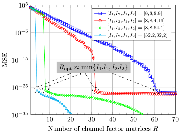
where 𝑩rI1×J1subscript𝑩𝑟superscriptsubscript𝐼1subscript𝐽1{\bm{B}}_{r}\in\mathbb{C}^{I_{1}\times J_{1}}, 𝑪rI2×J2subscript𝑪𝑟superscriptsubscript𝐼2subscript𝐽2{\bm{C}}_{r}\in\mathbb{C}^{I_{2}\times J_{2}}, I=I1I2𝐼subscript𝐼1subscript𝐼2I=I_{1}I_{2}, and J=J1J2𝐽subscript𝐽1subscript𝐽2J=J_{1}J_{2}. As shown in Fig. 3, the approximation becomes tighter as the number of channel factor matrices R𝑅R increases. More importantly, we can see that in case of full rank channels, the optimal value of R𝑅R, denoted in the figure by Roptsubscript𝑅optR_{\text{opt}}, is dependent on the division scenario of I𝐼I and J𝐽J, where Roptmin{I1J1,I2J2}subscript𝑅optsubscript𝐼1subscript𝐽1subscript𝐼2subscript𝐽2R_{\text{opt}}\approx\min\{I_{1}J_{1},I_{2}J_{2}\}. In other words, reducing the dimension of one of the channel factor matrices, i.e., 𝑩rI1×J1subscript𝑩𝑟superscriptsubscript𝐼1subscript𝐽1{\bm{B}}_{r}\in\mathbb{C}^{I_{1}\times J_{1}} or 𝑪rI2×J2subscript𝑪𝑟superscriptsubscript𝐼2subscript𝐽2{\bm{C}}_{r}\in\mathbb{C}^{I_{2}\times J_{2}}, reduces the value of Roptsubscript𝑅optR_{\text{opt}}.

Algorithm 1 Sequential Kronecker Factorization
1:Input: A matrix 𝑿I×J𝑿superscript𝐼𝐽{\bm{X}}\in\mathbb{C}^{I\times J}
2:Select R𝑅R, I1subscript𝐼1I_{1}, J1subscript𝐽1J_{1}, I2subscript𝐼2I_{2}, J2subscript𝐽2J_{2} such that I=I1I2𝐼subscript𝐼1subscript𝐼2I=I_{1}I_{2} and J=J1J2𝐽subscript𝐽1subscript𝐽2J=J_{1}J_{2}
3:for r=1𝑟1r=1 to R𝑅R do
4:     Get 𝑿r=𝑿r=1r1𝑿1,r𝑿2,rsubscript𝑿𝑟𝑿superscriptsubscriptsuperscript𝑟1𝑟1tensor-productsubscript𝑿1superscript𝑟subscript𝑿2superscript𝑟{\bm{X}}_{r}={\bm{X}}-\sum_{r^{\prime}=1}^{r-1}{\bm{X}}_{1,r^{\prime}}\otimes{\bm{X}}_{2,r^{\prime}}
5:     Given 𝑿rsubscript𝑿𝑟{\bm{X}}_{r}, get 𝑿1,rsubscript𝑿1𝑟{\bm{X}}_{1,r} and 𝑿2,rsubscript𝑿2𝑟{\bm{X}}_{2,r} using (11) and (12), respectively
6:end for
7:Output: ^X=r=1R𝑿1,r𝑿2,rI×Jbold-^absent𝑋superscriptsubscript𝑟1𝑅tensor-productsubscript𝑿1𝑟subscript𝑿2𝑟superscript𝐼𝐽{\bm{\hat{}}X}=\sum_{r=1}^{R}{\bm{X}}_{1,r}\otimes{\bm{X}}_{2,r}\in\mathbb{C}^{I\times J}
Refer to caption
Figure 3: MSE vs. the number of channel factor matrices R𝑅R assuming NBS=64subscript𝑁BS64N_{\text{BS}}=64, NUE=4subscript𝑁UE4N_{\text{UE}}=4, and NSC=16subscript𝑁SC16N_{\text{SC}}=16, where MSE=𝑯r=1R𝑪r𝑩rF2MSEsubscriptsuperscriptnorm𝑯superscriptsubscript𝑟1𝑅tensor-productsubscript𝑪𝑟subscript𝑩𝑟2F\text{MSE}=\|{\bm{H}}-\sum_{r=1}^{R}{\bm{C}}_{r}\otimes{\bm{B}}_{r}\|^{2}_{\text{F}}. Here, the total MIMO channel matrix 𝑯=[𝑯1,,𝑯NSC]I×J𝑯subscript𝑯1subscript𝑯subscript𝑁SCsuperscript𝐼𝐽{\bm{H}}=\big{[}\bm{H}_{1},\dots,\bm{H}_{N_{\text{SC}}}\big{]}\in\mathbb{C}^{I\times J} is generated following the 3GPP CDL channel model [19, 20] with the main system parameters outlined in Table I. Please refer to Section IV for more details.

Let L=TBSNRF𝐿subscript𝑇BSsubscript𝑁RFL=T_{\text{BS}}{N}_{\text{RF}}. Then, by substituting (14) into (6), and assuming R𝑅R is sufficiently large, we can write

𝒀𝒀\displaystyle{\bm{Y}} =𝑨(r=1R𝑪r𝑩r)+𝒁=r=1R𝑨(𝑪r𝑩r)+𝒁absent𝑨superscriptsubscript𝑟1𝑅tensor-productsubscript𝑪𝑟subscript𝑩𝑟𝒁superscriptsubscript𝑟1𝑅𝑨tensor-productsubscript𝑪𝑟subscript𝑩𝑟𝒁\displaystyle={\bm{A}}\Bigg{(}\sum_{r=1}^{R}{\bm{C}}_{r}\otimes{\bm{B}}_{r}\Bigg{)}+{\bm{Z}}=\sum_{r=1}^{R}{\bm{A}}({\bm{C}}_{r}\otimes{\bm{B}}_{r})+{\bm{Z}}
=r=1R𝒀r+𝒁L×J,absentsuperscriptsubscript𝑟1𝑅subscript𝒀𝑟𝒁superscript𝐿𝐽\displaystyle=\sum_{r=1}^{R}{\bm{Y}}_{r}+{\bm{Z}}\in\mathbb{C}^{L\times J}, (15)

where 𝒀r=𝑨(𝑪r𝑩r)L×Jsubscript𝒀𝑟𝑨tensor-productsubscript𝑪𝑟subscript𝑩𝑟superscript𝐿𝐽{\bm{Y}}_{r}={\bm{A}}({\bm{C}}_{r}\otimes{\bm{B}}_{r})\in\mathbb{C}^{L\times J}. From (III), we note that 𝒀rsubscript𝒀𝑟{\bm{Y}}_{r} can be seen as the 1-mode unfolding of a 3-way Tucker tensor given as [14]

𝓨r=𝓢×1𝑨×2𝑩r𝖳×3𝑪r𝖳L×J1×J2,subscript𝓨𝑟subscript3subscript2subscript1𝓢𝑨subscriptsuperscript𝑩𝖳𝑟subscriptsuperscript𝑪𝖳𝑟superscript𝐿subscript𝐽1subscript𝐽2\displaystyle\bm{\mathcal{Y}}_{r}=\bm{\mathcal{S}}\times_{1}{\bm{A}}\times_{2}{\bm{B}}^{\mathsf{T}}_{r}\times_{3}{\bm{C}}^{\mathsf{T}}_{r}\in\mathbb{C}^{L\times J_{1}\times J_{2}}, (16)

where 𝓢I×I1×I2𝓢superscript𝐼subscript𝐼1subscript𝐼2\bm{\mathcal{S}}\in\mathbb{Z}^{I\times I_{1}\times I_{2}} is the core-tensor with the 1-mode unfolding given as [𝓢](1)=def𝑰Isubscriptdelimited-[]𝓢1defsubscript𝑰𝐼[\bm{\mathcal{S}}]_{(1)}\overset{\text{def}}{=}{\bm{I}}_{I}. The \ell-mode unfolding of 𝓨rsubscript𝓨𝑟\bm{\mathcal{Y}}_{r}, ={1,2,3}123\ell=\{1,2,3\}, can be expressed as

[𝓨r](1)subscriptdelimited-[]subscript𝓨𝑟1\displaystyle[\bm{\mathcal{Y}}_{r}]_{(1)} =𝑨[𝓢](1)(𝑪r𝑩r)L×J,absent𝑨subscriptdelimited-[]𝓢1tensor-productsubscript𝑪𝑟subscript𝑩𝑟superscript𝐿𝐽\displaystyle={\bm{A}}[\bm{\mathcal{S}}]_{(1)}({\bm{C}}_{r}\otimes{\bm{B}}_{r})\in\mathbb{C}^{L\times J}, (17)
[𝓨r](2)subscriptdelimited-[]subscript𝓨𝑟2\displaystyle[\bm{\mathcal{Y}}_{r}]_{(2)} =𝑩r𝖳[𝓢](2)(𝑪r𝑨𝖳)J1×LJ2,absentsubscriptsuperscript𝑩𝖳𝑟subscriptdelimited-[]𝓢2tensor-productsubscript𝑪𝑟superscript𝑨𝖳superscriptsubscript𝐽1𝐿subscript𝐽2\displaystyle={\bm{B}}^{\mathsf{T}}_{r}[\bm{\mathcal{S}}]_{(2)}({\bm{C}}_{r}\otimes{\bm{A}}^{\mathsf{T}})\in\mathbb{C}^{J_{1}\times LJ_{2}}, (18)
[𝓨r](3)subscriptdelimited-[]subscript𝓨𝑟3\displaystyle[\bm{\mathcal{Y}}_{r}]_{(3)} =𝑪r𝖳[𝓢](3)(𝑩r𝑨𝖳)J2×LJ1.absentsubscriptsuperscript𝑪𝖳𝑟subscriptdelimited-[]𝓢3tensor-productsubscript𝑩𝑟superscript𝑨𝖳superscriptsubscript𝐽2𝐿subscript𝐽1\displaystyle={\bm{C}}^{\mathsf{T}}_{r}[\bm{\mathcal{S}}]_{(3)}({\bm{B}}_{r}\otimes{\bm{A}}^{\mathsf{T}})\in\mathbb{C}^{J_{2}\times LJ_{1}}. (19)

From (16), the 3-way Tucker tensor form of (III) can be expressed as

𝓨=r=1R𝓨r+𝓩L×J1×J2,𝓨superscriptsubscript𝑟1𝑅subscript𝓨𝑟𝓩superscript𝐿subscript𝐽1subscript𝐽2\displaystyle\bm{\mathcal{Y}}=\sum_{r=1}^{R}\bm{\mathcal{Y}}_{r}+\bm{\mathcal{Z}}\in\mathbb{C}^{L\times J_{1}\times J_{2}}, (20)

where 𝓩𝓩\bm{{{\mathcal{Z}}}} is the 3-way tensor representation of the noise matrix 𝒁𝒁{\bm{Z}}. This latter formulation suggests that the factor matrices {𝑩r,𝑪r}r=1Rsuperscriptsubscriptsubscript𝑩𝑟subscript𝑪𝑟𝑟1𝑅\{{\bm{B}}_{r},{\bm{C}}_{r}\}_{r=1}^{R} can be estimated sequentially as follows. Let 𝓨rsubscript𝓨𝑟\bm{\mathcal{Y}}_{r} be the tensor obtained at the r𝑟rth sequential step as

𝓨r=𝓨r=1r1𝓨rL×J1×J2.subscript𝓨𝑟𝓨superscriptsubscriptsuperscript𝑟1𝑟1subscript𝓨superscript𝑟superscript𝐿subscript𝐽1subscript𝐽2\displaystyle\bm{\mathcal{Y}}_{r}=\bm{\mathcal{Y}}-\sum_{r^{\prime}=1}^{r-1}\bm{\mathcal{Y}}_{r^{\prime}}\in\mathbb{C}^{L\times J_{1}\times J_{2}}. (21)

Then, by exploiting the 2-mode and the 3-mode unfoldings, the r𝑟rth factor matrices 𝑩rsubscript𝑩𝑟{\bm{B}}_{r} and 𝑪rsubscript𝑪𝑟{\bm{C}}_{r} can be obtained using, e.g., the ALS method [15], where one factor matrix is assumed to be fixed when solving for the other. Specifically, 𝑩rsubscript𝑩𝑟{\bm{B}}_{r} and 𝑪rsubscript𝑪𝑟{\bm{C}}_{r} can be obtained as

𝑩r𝖳subscriptsuperscript𝑩𝖳𝑟\displaystyle{\bm{B}}^{\mathsf{T}}_{r} =[𝓨r](2)[𝚿2]+=[𝓨r](2)𝚿2H[𝚿2𝚿2H]1absentsubscriptdelimited-[]subscript𝓨𝑟2superscriptdelimited-[]subscript𝚿2subscriptdelimited-[]subscript𝓨𝑟2superscriptsubscript𝚿2Hsuperscriptdelimited-[]subscript𝚿2superscriptsubscript𝚿2H1\displaystyle=[\bm{\mathcal{Y}}_{r}]_{(2)}\big{[}\bm{\Psi}_{2}\big{]}^{+}=[\bm{\mathcal{Y}}_{r}]_{(2)}{\bm{\Psi}}_{2}^{\text{H}}[{\bm{\Psi}}_{2}{\bm{\Psi}}_{2}^{\text{H}}]^{-1} (22)
𝑪r𝖳subscriptsuperscript𝑪𝖳𝑟\displaystyle{\bm{C}}^{\mathsf{T}}_{r} =[𝓨r](3)[𝚿3]+=[𝓨r](3)𝚿3H[𝚿3𝚿3H]1,absentsubscriptdelimited-[]subscript𝓨𝑟3superscriptdelimited-[]subscript𝚿3subscriptdelimited-[]subscript𝓨𝑟3superscriptsubscript𝚿3Hsuperscriptdelimited-[]subscript𝚿3superscriptsubscript𝚿3H1\displaystyle=[\bm{\mathcal{Y}}_{r}]_{(3)}\big{[}{\bm{\Psi}}_{3}\big{]}^{+}=[\bm{\mathcal{Y}}_{r}]_{(3)}{\bm{\Psi}}_{3}^{\text{H}}[{\bm{\Psi}}_{3}{\bm{\Psi}}_{3}^{\text{H}}]^{-1}, (23)

where 𝚿2subscript𝚿2{\bm{\Psi}}_{2} and 𝚿3subscript𝚿3{\bm{\Psi}}_{3} are given as

𝚿2subscript𝚿2\displaystyle{\bm{\Psi}}_{2} =[𝓢](2)(𝑪r𝑨𝖳)I1×LJ2absentsubscriptdelimited-[]𝓢2tensor-productsubscript𝑪𝑟superscript𝑨𝖳superscriptsubscript𝐼1𝐿subscript𝐽2\displaystyle=[\bm{\mathcal{S}}]_{(2)}({\bm{C}}_{r}\otimes{\bm{A}}^{\mathsf{T}})\in\mathbb{C}^{I_{1}\times LJ_{2}} (24)
𝚿3subscript𝚿3\displaystyle{\bm{\Psi}}_{3} =[𝓢](3)(𝑩r𝑨𝖳)I2×LJ1.absentsubscriptdelimited-[]𝓢3tensor-productsubscript𝑩𝑟superscript𝑨𝖳superscriptsubscript𝐼2𝐿subscript𝐽1\displaystyle=[\bm{\mathcal{S}}]_{(3)}({\bm{B}}_{r}\otimes{\bm{A}}^{\mathsf{T}})\in\mathbb{C}^{I_{2}\times LJ_{1}}. (25)

Algorithm 2 summarizes the proposed SALSA method for estimating the total MIMO channel matrix 𝑯I×J𝑯superscript𝐼𝐽{\bm{H}}\in\mathbb{C}^{I\times J}, which is guaranteed to converge monotonically to, at least, a local optimum solution [15].

Algorithm 2 SALSA For MIMO-OFDM Channel Estimation
1:Input: Measurement matrix 𝒀L×J𝒀superscript𝐿𝐽{\bm{Y}}\in\mathbb{C}^{L\times J} as in (6)
2:Select R1𝑅1R\geq 1, Nmax-iter1subscript𝑁max-iter1N_{\text{max-iter}}\geq 1, I1,I2,J1subscript𝐼1subscript𝐼2subscript𝐽1I_{1},I_{2},J_{1}, and J2subscript𝐽2J_{2} such that I=I1I2=NBS𝐼subscript𝐼1subscript𝐼2subscript𝑁BSI=I_{1}I_{2}={N}_{\text{BS}} and J=J1J2=NUENSC𝐽subscript𝐽1subscript𝐽2subscript𝑁UEsubscript𝑁SCJ=J_{1}J_{2}={N}_{\text{UE}}N_{\text{SC}}
3:Obtain the 3-way Tucker tensor 𝓨𝓨\bm{\mathcal{Y}} in (20) from 𝒀𝒀{\bm{Y}}
4:for r=1𝑟1r=1 to R𝑅R do
5:     Get 𝓨r=𝓨r=1r1𝓨^rsubscript𝓨𝑟𝓨superscriptsubscriptsuperscript𝑟1𝑟1subscriptbold-^𝓨superscript𝑟\bm{\mathcal{Y}}_{r}=\bm{\mathcal{Y}}-\sum_{r^{\prime}=1}^{r-1}\bm{\mathcal{\hat{Y}}}_{r^{\prime}}
6:     Initialize 𝑪r(0)I2×J2subscriptsuperscript𝑪0𝑟superscriptsubscript𝐼2subscript𝐽2{\bm{C}}^{(0)}_{r}\in\mathbb{C}^{I_{2}\times J_{2}}, e.g., randomly
7:     for n=1𝑛1n=1 to Nmax-itersubscript𝑁max-iterN_{\text{max-iter}} do
8:         Get 𝑩r(n)subscriptsuperscript𝑩𝑛𝑟{\bm{B}}^{(n)}_{r} using (22) for given 𝑪r(n1)subscriptsuperscript𝑪𝑛1𝑟{\bm{C}}^{(n-1)}_{r}
9:         Get 𝑪r(n)subscriptsuperscript𝑪𝑛𝑟{\bm{C}}^{(n)}_{r} using (23) for given 𝑩r(n)subscriptsuperscript𝑩𝑛𝑟{\bm{B}}^{(n)}_{r}
10:     end for
11:     Set 𝑩^r=𝑩r(Nmax-iter)subscriptbold-^𝑩𝑟subscriptsuperscript𝑩subscript𝑁max-iter𝑟\bm{\hat{B}}_{r}={\bm{B}}^{(N_{\text{max-iter}})}_{r} and 𝑪^r=𝑪r(Nmax-iter)subscriptbold-^𝑪𝑟subscriptsuperscript𝑪subscript𝑁max-iter𝑟\bm{\hat{C}}_{r}={\bm{C}}^{(N_{\text{max-iter}})}_{r}
12:     Get 𝓨^r=𝓢×1𝑨×2𝑩^r𝖳×3𝑪^r𝖳subscriptbold-^𝓨𝑟subscript3subscript2subscript1𝓢𝑨subscriptsuperscriptbold-^𝑩𝖳𝑟subscriptsuperscriptbold-^𝑪𝖳𝑟\bm{\mathcal{\hat{Y}}}_{r}=\bm{\mathcal{S}}\times_{1}{\bm{A}}\times_{2}\bm{\hat{B}}^{\mathsf{T}}_{r}\times_{3}\bm{\hat{C}}^{\mathsf{T}}_{r}, go back to Step (5)
13:end for
14:Output: 𝑯^SALSA=r=1R𝑪^r𝑩^rI×Jsubscriptbold-^𝑯SALSAsuperscriptsubscript𝑟1𝑅tensor-productsubscriptbold-^𝑪𝑟subscriptbold-^𝑩𝑟superscript𝐼𝐽\bm{\hat{H}}_{\text{SALSA}}=\sum_{r=1}^{R}\bm{\hat{C}}_{r}\otimes\bm{\hat{B}}_{r}\in\mathbb{C}^{I\times J}

Note that, due to the right filtering, the SALSA method in Algorithm 2 requires that (C1) I1LJ2subscript𝐼1𝐿subscript𝐽2I_{1}\leq LJ_{2} and (C2) I2LJ1subscript𝐼2𝐿subscript𝐽1I_{2}\leq LJ_{1}, i.e., TBSmin{I1NRFJ2,I2NRFJ1}subscript𝑇BSsubscript𝐼1subscript𝑁RFsubscript𝐽2subscript𝐼2subscript𝑁RFsubscript𝐽1T_{\text{BS}}\geq\min\Big{\{}\frac{I_{1}}{{N}_{\text{RF}}J_{2}},\frac{I_{2}}{{N}_{\text{RF}}J_{1}}\Big{\}} to provide an accurate channel estimation. Therefore, under practical settings, the SALSA method in Algorithm 2 requires less training overhead than the LS method in (7). On the other hand, assuming that the complexity of calculating the Moore-Penrose pseudo-inverse of an n×m𝑛𝑚n\times m matrix is on the order of 𝒪(min{n,m}3)\mathcal{O}(\min\{n,m\}^{3}), then the complexity of the LS method in (7) is on the order of 𝒪(min{L,J})3𝒪superscript𝐿𝐽3\mathcal{O}(\min\{L,J\})^{3}, while for the SALSA method in Algorithm 2 the complexity is on the order of 𝒪(RNmax-iterI13I23)𝒪𝑅subscript𝑁max-itersuperscriptsubscript𝐼13superscriptsubscript𝐼23\mathcal{O}(R\cdot N_{\text{max-iter}}\cdot I_{1}^{3}\cdot I_{2}^{3}), assuming that the (C1) and (C2) conditions are satisfied.

IV Simulation Results

We adopt the 3GPP clustered delay line (CDL) channel model described in TR 38.901 [19], where a step-by-step tutorial of it along the MATLAB scripts for channel generation is presented in [20]. Specifically, in our simulation, we first generate a time-domain channel tensor 𝓗NBS×NUE×Ntaps𝓗superscriptsubscript𝑁BSsubscript𝑁UEsubscript𝑁taps\bm{\mathcal{H}}\in\mathbb{C}^{N_{\text{BS}}\times N_{\text{UE}}\times N_{\text{taps}}}, where Ntapssubscript𝑁tapsN_{\text{taps}} represents the number of time-domain channel taps calculated according to [20, Eqn. (64)] and using the system parameters shown in Table I. Then, we perform a NSCsubscript𝑁SCN_{\text{SC}}-point FFT operation along the third dimension for each receive-transmit antenna pair to obtain the frequency-domain channel tensor 𝓗NBS×NUE×NSC𝓗superscriptsubscript𝑁BSsubscript𝑁UEsubscript𝑁SC\bm{\mathcal{H}}\in\mathbb{C}^{N_{\text{BS}}\times N_{\text{UE}}\times N_{\text{SC}}}, where the k𝑘kth slice matrix 𝑯k=𝓗[:,:,k]NBS×NUEsubscript𝑯𝑘subscript𝓗::𝑘superscriptsubscript𝑁BSsubscript𝑁UE\bm{H}_{k}=\bm{\mathcal{H}}_{[:,:,k]}\in\mathbb{C}^{N_{\text{BS}}\times N_{\text{UE}}} represents the the k𝑘kth subcarrier frequency-domain MIMO channel matrix.

We show the simulation results in terms of the normalized mean-square-error (NMSE) that is defined as NMSE=𝔼{𝑯𝑯^XF2}/𝔼𝑯F2}\text{NMSE}=\mathbb{E}\{\|{\bm{H}}-\bm{\hat{H}}_{\text{X}}\|_{\text{F}}^{2}\}/\mathbb{E}\|{\bm{H}}\|_{\text{F}}^{2}\}, where X{LS, SALSA}XLS, SALSA\text{X}\in\{\text{LS, SALSA}\}. The signal-to-noise ratio (SNR) is defined as SNR=𝔼{𝓨𝓩F2}/𝔼{𝓩F2}SNR𝔼superscriptsubscriptnorm𝓨𝓩F2𝔼superscriptsubscriptnorm𝓩F2\text{SNR}=\mathbb{E}\{\|\bm{\mathcal{Y}}-\bm{\mathcal{Z}}\|_{\text{F}}^{2}\}/\mathbb{E}\{\|\bm{\mathcal{Z}}\|_{\text{F}}^{2}\}. In all simulation scenarios, we set NBS=64subscript𝑁BS64N_{\text{BS}}=64, NUE=4subscript𝑁UE4N_{\text{UE}}=4, NSC=16subscript𝑁SC16N_{\text{SC}}=16, TUE=NUEsubscript𝑇UEsubscript𝑁UET_{\text{UE}}=N_{\text{UE}}, NRF=4subscript𝑁RF4N_{\text{RF}}=4, NG=2subscript𝑁G2N_{\text{G}}=2, and assume a random generation of the analog decoding matrix 𝑨TBSNRF×NBS𝑨superscriptsubscript𝑇BSsubscript𝑁RFsubscript𝑁BS\bm{A}\in\mathbb{C}^{T_{\text{BS}}{N}_{\text{RF}}\times N_{\text{BS}}}, where every nonzero entry is obtained as a=1/N̊BSejϕ𝑎1subscript̊𝑁BSsuperscript𝑒𝑗italic-ϕa={1}/{\sqrt{\mathring{N}_{\text{BS}}}}\cdot e^{j\phi}, where ϕ[0,2π]italic-ϕ02𝜋\phi\in[0,2\pi].

TABLE I: System Parameters
Parameter Value
Scenario UMi
Cell radius 100 m
BS (UE) height 10 (1.5) m
Carrier frequency fcsubscript𝑓𝑐f_{c} 4 GHz
Sampling frequency fssubscript𝑓𝑠f_{s} 30.72 MSamples/s
No. of subcarriers NSCsubscript𝑁SCN_{\text{SC}} 161616
No. of antennas at BS NBSsubscript𝑁BSN_{\text{BS}} 64 (8×8)88(8\times 8)
No. of antennas at UE NUEsubscript𝑁UEN_{\text{UE}} 4 (2×2)22(2\times 2)
Polarization Single
Refer to caption
Refer to caption
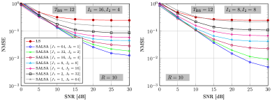
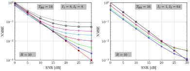
Figure 4: NMSE vs. SNR for different I𝐼I and J𝐽J division scenarios.

Initially, we show simulation results investigating the best division scenario of I𝐼I and J𝐽J with the constraints of I=I1I2𝐼subscript𝐼1subscript𝐼2I=I_{1}I_{2}, J=J1J2𝐽subscript𝐽1subscript𝐽2J=J_{1}J_{2}, Id1subscript𝐼𝑑1I_{d}\geq 1, Jd1subscript𝐽𝑑1J_{d}\geq 1, and Id,Jdsubscript𝐼𝑑subscript𝐽𝑑I_{d},J_{d} are Natural numbers, where d{1,2}𝑑12d\in\{1,2\}. Recall that I=NBS𝐼subscript𝑁BSI={N}_{\text{BS}} and J=NUENSC𝐽subscript𝑁UEsubscript𝑁SCJ={N}_{\text{UE}}N_{\text{SC}}. Therefore, we have I=J=64𝐼𝐽64I=J=64 and the candidate numbers of Idsubscript𝐼𝑑I_{d} and Jdsubscript𝐽𝑑J_{d} are 1,2,4,8,16,32124816321,2,4,8,16,32, and 646464. Therefore, we have in total 49 different division scenarios as illustrated in Table II. We have simulated the SALSA algorithm using all the 49 possible scenarios. In Fig. 4, we show the NMSE versus SNR results for some selected I𝐼I and J𝐽J division scenarios. The other scenarios are not shown, due to space limitations, but we note that their NMSE performance are inferior compared to the shown scenarios.

From Fig. 4, when TBS=12subscript𝑇BS12T_{\text{BS}}=12, i.e., L=TBSNRF=48<NBS𝐿subscript𝑇BSsubscript𝑁RF48subscript𝑁BSL=T_{\text{BS}}{N}_{\text{RF}}=48<N_{\text{BS}}, the analog training matrix 𝑨L×NBS𝑨superscript𝐿subscript𝑁BS\bm{A}\in\mathbb{C}^{L\times N_{\text{BS}}}, i.e., the 1st factor matrix of the measurement tensor in (16), is left non-invertible, i.e., [𝑨]+𝑨𝑰superscriptdelimited-[]𝑨𝑨𝑰[{\bm{A}}]^{+}{\bm{A}}\neq\bm{I}. Therefore, the LS-based method has a very bad channel estimation accuracy NMSE. On the other hand, we can see that the best NMSE of SALSA method is achieved when I1=8subscript𝐼18I_{1}=8, I2=8subscript𝐼28I_{2}=8, J1=64subscript𝐽164J_{1}=64, and J2=1subscript𝐽21J_{2}=1, i.e., when 𝑩r8×64subscript𝑩𝑟superscript864{\bm{B}}_{r}\in\mathbb{C}^{8\times 64} and 𝑪r8×1,rsubscript𝑪𝑟superscript81for-all𝑟{\bm{C}}_{r}\in\mathbb{C}^{8\times 1},\forall r. The main reason is that by dividing I=64𝐼64I=64 equally between I1subscript𝐼1I_{1} and I2subscript𝐼2I_{2}, i.e., I1=I2=8subscript𝐼1subscript𝐼28I_{1}=I_{2}=8, SALSA reduces the impact of the non-invertibility of 𝑨𝑨\bm{A} by distributing it between the 2nd (i.e., 𝑩rsubscript𝑩𝑟{\bm{B}}_{r}) and the 3rd (i.e., 𝑪rsubscript𝑪𝑟{\bm{C}}_{r}) factor matrices of the measurement tensor, which leads to a better channel estimation accuracy. On the other hand, by setting J1=64subscript𝐽164J_{1}=64 and J2=1subscript𝐽21J_{2}=1, the required number of channel factor matrices R𝑅R reduces as compared to the other division scenario, as we have illustrated above in Fig. 3.

Differently, when TBS=16subscript𝑇BS16T_{\text{BS}}=16, i.e., L=NBS𝐿subscript𝑁BSL=N_{\text{BS}}, the analog training matrix 𝑨𝑨\bm{A} is left invertible, i.e., [𝑨]+𝑨=𝑰superscriptdelimited-[]𝑨𝑨𝑰[{\bm{A}}]^{+}{\bm{A}}=\bm{I}. Therefore, the LS-based method has an accurate channel estimation accuracy. For SALSA method, on the other hand, we can see that when I1=8subscript𝐼18I_{1}=8 and I2=8subscript𝐼28I_{2}=8, the estimation accuracy of SALSA improves as we increase J1subscript𝐽1J_{1} and decrease J2subscript𝐽2J_{2}, where the best result is obtained when we have J1=64subscript𝐽164J_{1}=64 and J2=1subscript𝐽21J_{2}=1, i.e., similar to the case above when TBS=12subscript𝑇BS12T_{\text{BS}}=12. Nonetheless, we can see that the SALSA method can obtain a more accurate channel estimation, compered to the LS-based method, by setting I1=1subscript𝐼11I_{1}=1, I2=64subscript𝐼264I_{2}=64, J1=64subscript𝐽164J_{1}=64, and J2=1subscript𝐽21J_{2}=1, i.e., 𝑩r1×64subscript𝑩𝑟superscript164{\bm{B}}_{r}\in\mathbb{C}^{1\times 64} and 𝑪r64×1subscript𝑪𝑟superscript641{\bm{C}}_{r}\in\mathbb{C}^{64\times 1} (or, not shown in the figure, by setting I1=64subscript𝐼164I_{1}=64, I2=1subscript𝐼21I_{2}=1, J1=1subscript𝐽11J_{1}=1, and J2=64subscript𝐽264J_{2}=64, i.e., 𝑩r64×1subscript𝑩𝑟superscript641{\bm{B}}_{r}\in\mathbb{C}^{64\times 1} and 𝑪r1×64subscript𝑪𝑟superscript164{\bm{C}}_{r}\in\mathbb{C}^{1\times 64}). In the both these scenarios, the channel matrix 𝑯64×64𝑯superscript6464\bm{H}\in\mathbb{C}^{64\times 64} in (14) is decomposed into a summation of R𝑅R factor matrices 𝑩r𝑪r64×64tensor-productsubscript𝑩𝑟subscript𝑪𝑟superscript6464{\bm{B}}_{r}\otimes{\bm{C}}_{r}\in\mathbb{C}^{64\times 64}, each having a rank-one, i.e., rank{𝑩r𝑪r}=1,rtensor-productsubscript𝑩𝑟subscript𝑪𝑟1for-all𝑟\{{\bm{B}}_{r}\otimes{\bm{C}}_{r}\}=1,\forall r, which leads to a better channel estimation accuracy.

TABLE II: Division scenarios of I1,I2,J1subscript𝐼1subscript𝐼2subscript𝐽1I_{1},I_{2},J_{1}, and J2subscript𝐽2J_{2}
Scenario No. I1subscript𝐼1I_{1} and I2subscript𝐼2I_{2} values J1subscript𝐽1J_{1} and J2subscript𝐽2J_{2} values
Scenario 1 [I1,I2]=[64,1]subscript𝐼1subscript𝐼2641[I_{1},I_{2}]=[64,1] [J1,J2]=[64,1]subscript𝐽1subscript𝐽2641[J_{1},J_{2}]=[64,1]
\vdots
Scenario 7 [J1,J2]=[1,64]subscript𝐽1subscript𝐽2164[J_{1},J_{2}]=[1,64]
\vdots \vdots \vdots
Scenario 43 [I1,I2]=[1,64]subscript𝐼1subscript𝐼2164[I_{1},I_{2}]=[1,64] [J1,J2]=[64,1]subscript𝐽1subscript𝐽2641[J_{1},J_{2}]=[64,1]
\vdots
Scenario 49 [J1,J2]=[1,64]subscript𝐽1subscript𝐽2164[J_{1},J_{2}]=[1,64]

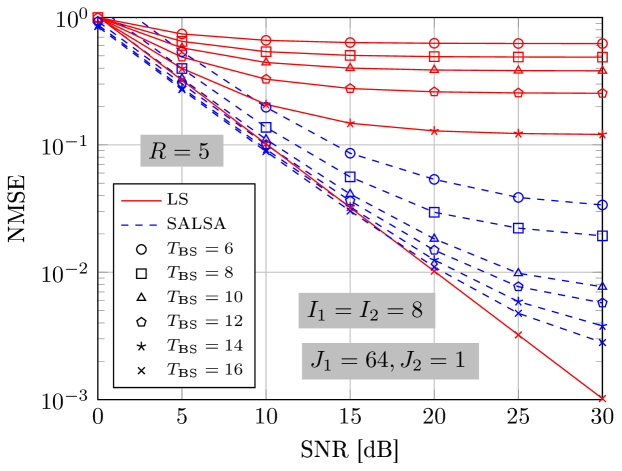
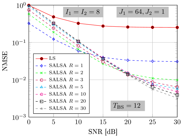
In Figs. 5 and 6 we show NMSE versus SNR simulation results with varying the number of channel training overhead, i.e., TBSsubscript𝑇BST_{\text{BS}} and the number of channel factor matrices, i.e., R𝑅R, respectively. From Fig. 5, we can see that the channel estimation accuracy of both methods, i.e., LS-based and SALSA improves as TBSsubscript𝑇BST_{\text{BS}} increases. However, SALSA significantly outperforms LS-based with all TBS<16subscript𝑇BS16T_{\text{BS}}<16, i.e., L<NBS𝐿subscript𝑁BSL<N_{\text{BS}} scenarios, wherein the analog training matrix 𝑨L×NBS𝑨superscript𝐿subscript𝑁BS\bm{A}\in\mathbb{C}^{L\times N_{\text{BS}}} is left non-invertible.

On the other hand, we can see from Fig. 6 that the SALSA channel estimation accuracy increases with the increasing R𝑅R, in the high SNR regime, while it decreases with the increasing R𝑅R, in the low SNR regime. The main reason is that, in the high SNR regime, the noise impact is minimal and by increasing R𝑅R, the channel estimation accuracy increases, as we have illustrated above in Fig. 3. On the other hand, in the low SNR regime, the channel measurement tensor is noise-limited and, therefore, the impact of noise increases by increasing R𝑅R, i.e., after a certain R𝑅R, the estimated channel factor matrices are very noisy that decreases the overall estimation accuracy. Clearly, for every SNR regime/level, there is an optimal R𝑅R value, wherein the channel estimation accuracy is maximized, which we leave for a follow up future work.
Refer to caption
Figure 5: NMSE vs. SNR with varying TBSsubscript𝑇BST_{\text{BS}}.
Refer to caption
Figure 6: NMSE vs. SNR with varying R𝑅R.

V Conclusion

In this paper, we have proposed a novel channel estimation method for MIMO-OFDM sub-6 GHz communication systems called SALSA. We have shown that an accurate channel estimation can be obtained with a small training overhead by exploiting a hidden tensor structure in the received measurement matrix, which estimates the channel matrix sequentially using an ALS-based method. Our results show that the SALSA method outperforms the conventional LS-based method, especially in the low training overhead, which makes it more appealing for practical implementations.

References

  • [1] T. L. Marzetta, E. G. Larsson, H. Yang, and H. Q. Ngo, Fundamentals of Massive MIMO.   Cambridge University Press, 2016.
  • [2] E. Dahlman, S. Parkvall, and J. Skold, 5G NR: The Next Generation Wireless Access Technology, 1st ed.   USA: Academic Press, Inc., 2018.
  • [3] E. Björnson, L. Sanguinetti, J. Hoydis, and M. Debbah, “Optimal design of energy-efficient multi-user MIMO systems: Is massive MIMO the answer?” IEEE Trans. Wireless Commun., vol. 14, no. 6, pp. 3059–3075, Jun. 2015.
  • [4] R. W. Heath, N. González-Prelcic, S. Rangan, W. Roh, and A. M. Sayeed, “An overview of signal processing techniques for Millimeter Wave MIMO systems,” IEEE Journal of Selected Topics in Signal Processing, vol. 10, no. 3, pp. 436–453, 2016.
  • [5] K. Ardah, G. Fodor, Y. C. B. Silva, W. Cruz, and F. R. Cavalcanti, “A unifying design of hybrid beamforming architectures employing phase-shifters or switches,” IEEE Trans. Veh. Technol., pp. 1–1, 2018.
  • [6] X. Gao, L. Dai, S. Han, C.-L. I, and R. W. Heath, “Energy-efficient hybrid analog and digital precoding for MmWave MIMO systems with large antenna arrays,” IEEE Journal on Selected Areas in Communications, vol. 34, no. 4, pp. 998–1009, 2016.
  • [7] H. Shokri-Ghadikolaei, C. Fischione, G. Fodor, P. Popovski, and M. Zorzi, “Millimeter wave cellular networks: A MAC layer perspective,” IEEE Transactions on Communications, vol. 63, no. 10, pp. 3437–3458, 2015.
  • [8] S. Gherekhloo, K. Ardah, and M. Haardt, “Hybrid beamforming design for downlink MU-MIMO-OFDM millimeter-wave systems,” in Proc. IEEE 11th Sensor Array and Multichannel Signal Processing Workshop (SAM), 2020, pp. 1–5.
  • [9] A. Alkhateeb, G. Leus, and R. W. Heath, “Compressed sensing based multi-user millimeter wave systems: How many measurements are needed?” in Proc. IEEE International Conference on Acoustics, Speech and Signal Processing (ICASSP), 2015, pp. 2909–2913.
  • [10] K. Ardah, B. Sokal, A. L. F. de Almeida, and M. Haardt, “Compressed sensing based channel estimation and open-loop training design for hybrid analog-digital massive MIMO systems,” in Proc. 2020 IEEE International Conference on Acoustics, Speech and Signal Processing (ICASSP), 2020, pp. 4597–4601.
  • [11] J. Zhang and M. Haardt, “Channel estimation and training design for hybrid multi-carrier mmwave massive MIMO systems: The beamspace ESPRIT approach,” in Proc. 25th European Signal Processing Conference (EUSIPCO), 2017, pp. 385–389.
  • [12] I. Barhumi, G. Leus, and M. Moonen, “Optimal training design for MIMO OFDM systems in mobile wireless channels,” IEEE Transactions on Signal Processing, vol. 51, no. 6, pp. 1615–1624, 2003.
  • [13] M. Biguesh and A. Gershman, “Training-based MIMO channel estimation: a study of estimator tradeoffs and optimal training signals,” IEEE Transactions on Signal Processing, vol. 54, no. 3, pp. 884–893, 2006.
  • [14] M. Haardt, F. Roemer, and G. Del Galdo, “Higher-order SVD-based subspace estimation to improve the parameter estimation accuracy in multidimensional harmonic retrieval problems,” IEEE Transactions on Signal Processing, vol. 56, no. 7, pp. 3198–3213, 2008.
  • [15] P. Comon, X. Luciani, and A. L. F. de Almeida, “Tensor decompositions, alternating least squares and other tales,” Journal of Chemometrics, vol. 23, no. 7-8, pp. 393–405, 2009.
  • [16] C. F. Van Loan and N. Pitsianis, Approximation with Kronecker Products, M. S. Moonen, G. H. Golub, and B. L. R. De Moor, Eds.   Dordrecht: Springer Netherlands, 1993.
  • [17] K. K. Wu, Y. Yam, H. Meng, and M. Mesbahi, “Kronecker product approximation with multiple factor matrices via the tensor product algorithm,” in Proc. IEEE International Conference on Systems, Man, and Cybernetics (SMC), 2016, pp. 004 277–004 282.
  • [18] C. Garvey, C. Meng, and J. G. Nagy, “Singular value decomposition approximation via kronecker summations for imaging applications,” 2018. [Online]. Available: https://arxiv.org/abs/1803.11525
  • [19] 3GPP, “Study on Channel Model for Frequencies from 0.5 to 100 GHz,” 3rd Generation Partnership Project (3GPP), Technical Report (TR) 38.901, 2020, v16.1.0.
  • [20] D. G. Riviello, F. Di Stasio, and R. Tuninato, “Performance analysis of multi-user MIMO schemes under realistic 3GPP 3-D channel model for 5G mmwave cellular networks,” Electronics, vol. 11, no. 3, 2022. [Online]. Available: https://www.mdpi.com/2079-9292/11/3/330