Chaotic interactions between dark matter and dark energy

Abstract

In this study, we consider dark matter and dark energy as grand-canonical systems which are open, non-equilibrium coupled, and interacting systems. First time, we propose a new more realistic interaction schema to explain dynamics between coupled interacting thermodynamic systems. Based on this new interaction schema, we propose new theorems to define the interactions including mutual and self-interactions. We proved the theorems based on the energy conservation law of thermodynamics. Furthermore, we obtain new coupled equations using the theorems. We numerically solved the interaction equations and obtained phase space diagrams and Lyapunov exponents. We show that the interaction between dark matter and dark energy is chaotic. We conclude that these theorems and results can be generalized to all coupled interacting particle and thermodynamic systems. Finally, we evaluated that the obtained results indicate the existence of a new law in physics. Additionally, based on the results, we gave physical definitions of basic concepts such as chaos and self-organization and pointed out the existence of hidden symmetries and variables in interacting systems.

I Introduction

It is known that our universe, which continues to expand, consists not only of matter but also of dark matter and dark energy. Dark matter, which is thought to interact with matter only through gravity, was proposed to explain the rotational anomaly of galaxies [1, 2, 3]. Later, the acceleration of the expansion of the universe was first discovered by Riess et al. [4] by measuring luminosity distances of SNe Ia, used as standard candles. Perlmutter et al. [5] later confirmed the discovery with analysis of nearby and high-redshift supernovae. Today, we know that our universe is composed of about %71.4 dark energy, %24 dark matter, and %4.6 regular matter (according to WMAP data) [6, 7]. However, dark energy is approximately %68.3, dark matter is %26.8, and matter is approximately %4.9 (according to Planck data) [8].

Although the physical origin of dark matter and dark energy has not been explained yet, it is known that they play an important role in the dynamics of the universe. For this reason, the interaction of all the components that make up the universe and understanding the results arising from these interactions is one of the most important problems of cosmology. Therefore, so far, many interacting models based on dark matter and dark energy interaction have been used to solve the singularity and cosmic coincidence problems [9, 10, 11, 12, 13, 14, 15, 16, 17, 18, 19, 20, 21, 22, 23, 24, 25, 26, 27, 28, 29, 12, 13, 30, 31, 32, 33, 34, 35, 36, 37, 38, 39].

In 2018, we proposed a new interactions schema among the components such as matter, dark matter, and dark energy based on Lotka-Volterra-like equations [38]. In that study, we show that the interaction dynamics of these components are chaotic. Motivated by these results, we suggest that the universe is evolving chaotically within the cosmic time-line. We conclude that new cosmology theory has the potential to solve many complications of the big-bang cosmology such as singularity, cosmic coincidence, emergence of the galaxies, fractal formation of the universe from micro to macro scale, and future and end of the universe. Later, based on dark matter and dark energy interactions, we explain the transition from a matter-dominated era to a dark energy-dominated era [39]. Furthermore, we carried out that this transition appears around 9.8-10 Gyears in the cosmic timeline and give a hybrid scale factor that defines both eras, precisely.

Here, it should be noted that although Lotka-Volterra type equations can cause chaotic behavior under some special conditions [38, 40, 41, 42], we cannot say that such equations do not recognize the interaction between dark matter and dark energy accurately enough. Therefore, in this study, we will propose a new interaction schema for coupled open systems to provide their main claim in Ref. [38]. Furthermore, we will consider dark matter and dark energy as an open and interacting thermodynamic system in a new interaction schema, unlike standard statistical thermodynamics. Based on this new theoretical framework, we will show that interaction equations can be derived from the first law of thermodynamics. To obtain a full description of the interaction we will suggest a new complementary equation by inspired graph theory. Finally, based on these theorems, we will carry out new interaction equations that describe the interaction between dark matter and dark energy. We show that interactions between dark matter and dark energy is chaotic. Our results may make a critical contribution not only to cosmology but also to the statistical thermodynamics and understanding of nature and living systems.

This work is organized as follows: In Section II, we briefly give the conventional method for modeling dark matter and dark energy interaction. In Section III, we introduce a new and novel interaction schema to model dark matter and dark energy interactions. We introduce new theorems and give proofs based on the energy conservation law of thermodynamics. We obtain new interaction equations between coupling non-equilibrium systems. In Section IV, the numerical solution of the new model is given. We present some remarkable conclusions in Section V. Finally, we summarize the important results in the last section.

II The Conventional Approach to the Interaction

We know that dark matter and dark energy coexist in the Universe. The continuity equation for both dark matter and dark energy is given by

$$\dot{\rho}+3H\left(\rho+p\right)=0.$$ (1)

If we assume that they should be interacts in the same volume, the continuity equation (1) can be written for the dark matter and dark energy as

$$\frac{d\rho_{dm}}{dt}+3H\left(\rho_{dm}+p_{dm}\right)=X$$ (2a)

$$\frac{d\rho_{de}}{dt}+3H\left(\rho_{de}+p_{de}\right)=-X$$ (2b)

where $X$ is the interaction coupling term. In the interaction models, interaction coupling term $X$ has been chosen differently.

So far many different interaction models have been proposed in literature. For example, in our previous study [38], we consider $X=\gamma\rho_{dm}\rho_{de}$ where $\gamma$ is the interaction constant. By setting $\alpha_{1}=3H(1+w_{dm})$, $\alpha_{2}=-3H(1+w_{de})$, $x_{1}=\frac{\gamma}{\alpha_{2}}\rho_{dm}$ and $x_{2}=\frac{\gamma}{\alpha_{1}}\rho_{de}$, Eq.(2) can be written in terms of Lotka-Volterra equation [38]:

$$\frac{dx_{1}}{dt}=\alpha_{1}x_{1}\left(1-x_{2}\right)$$ (3a)

$$\frac{dx_{2}}{dt}=\alpha_{2}x_{2}\left(x_{1}-1\right)$$ (3b)

where $\alpha_{1,2}$ are the interaction rate parameters.

The phase space solution is periodic of the Lotka-Volterra equation in Eq.(3). Based on this idea, in the previous study [38], it was extended Eq.(3) to more general interaction presentation by adding quadratic term which represent self-interaction

$$\frac{dx_{i}}{dt}=x_{i}\sum_{j}^{N}\alpha_{ij}\left(1-x_{j},\right)\qquad i=1,...,N$$ (4)

which is the same equation in Ref.[40, 41]. It was shown that the solutions obtained from the coupled density equations already show that the dynamics of the system is chaotic. In his approach, different components or kinds are consume each other. However, this approach may violates the conservation laws. Therefore, we say that this interaction method is in-completed the point of view of statistical thermodynamics. We will present a new method which cover the full thermodynamic behavior of the interacting system.

III New Interaction Theory

We consider the dark matter and dark energy as the grand canonical thermodynamic systems. According to conventional approach, they interact in the Universe by exchanging energy and particles as seen in Fig.1.

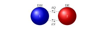
Figure 1: The schematic picture for the thermodynamic ensemble of the dark matter (DM) and dark energy (DE). In the standard thermodynamic schema, open thermodynamic ensembles interact via the $\delta Q$ and $\delta N$ exchange. Here we set $dV=0$.

However, we show that the conventional approach is not enough to define the interactions between two open, coupled non-equilibrium thermodynamic systems. Therefore, we introduce new interaction schema and theorems to define the correct interactions equations. Below, for simplicity we label dark matter and dark energy as system $1$ and $2$, respectively.

III.1 Mutual Interactions

Lemma 1

The continuity equation for a non-equilibrium system $1$ which interacts the system $2$ should be presented form as

$$\frac{d\rho_{1}}{dt}+3H\left(\rho_{1}+p_{1}\right)=\frac{dX_{2}}{dt}$$ (5)

where $X_{2}$ is the source system $2$ based on Prigogine approach [43].

Change of the source $X_{2}$ can be defined as $X_{2}=\Gamma_{1}N_{2}$ where $N_{2}$ is the source system, $\Gamma_{1}$ denotes energy transfer rates of the system $1$ which determines the energy amount which is transferred the from system $2$ to the system $1$. In the present study, based on this Lemma, we present a new interaction schema and new theorems.

Theorem 1

The interactions between two coupled non-equilibrium system can be obtained the energy conservation law of the statistical thermodynamics and is given in a simple form as

$$\frac{dx_{1}}{dt}=\Gamma_{1}x_{2}-x_{1}$$ (6a)

$$\frac{dx_{2}}{dt}=\Gamma_{2}x_{1}-x_{2}$$ (6b)

where $x_{1,2}$ denote energy flux between systems and $\Gamma_{1,2}$ energy transfer rates which are time-dependent degrees of freedom of the system.

Proof: The two open and coupled interacting system $1$ and $2$ is given in Fig.1. In the standard statistical thermodynamics, the open and interacting two systems are characterized by the energy and particle exchange as in Fig.1. The energy conservation law of thermodynamics for any open thermodynamic systems is given by

$$dU=\delta Q-pdV-\mu dN$$ (7)

where $dU$ corresponds to energy exchange in the system, $\delta Q$ is heat changes, $p$ is pressure, $dV$ denotes volume exchange, $\mu$ is the chemical potential and $dN$ is the particle exchange in the same system.

For the constant volume $dV=0$, the energy conservation laws of the thermodynamics for two non-interacting system are given separately as

$$dU_{1}=dQ_{1}-\mu_{1}dN_{1}$$ (8a)

$$dU_{2}=dQ_{2}-\mu_{2}dN_{2}$$ (8b)

These equation can be represent as time-dependent form

$$\frac{dU_{1}}{dt}=\frac{dQ_{1}}{dt}-\mu_{1}\frac{dN_{1}}{dt}$$ (9a)

$$\frac{dU_{2}}{dt}=\frac{dQ_{2}}{dt}-\mu_{2}\frac{dN_{2}}{dt}$$ (9b)

It should be noted that these equations do not represent the interaction between systems, however, they denote only independent energy change in two systems in contact with each other. It is a conventional mistake to say that the interactions between two thermodynamic systems are given by Eq.(9).

In order to write the interaction between two systems, it is necessary to accept that the two systems couple. The interaction naturally connects the two systems and the flow of energy occurs between the two systems. The energy flow between the two systems must be bidirectional, as shown in Fig.2(a), due to the nature of the interaction. This exchange represents mutual interaction. The energy fluxes $x_{1}$ and $x_{2}$ in Fig.2.(a) can be determined by Eq.(9). As we will show below these fluxes represent the changes in $\delta Q$ and $\delta N$ between the two systems in terms of energy. However, it is not enough to assume that the energy flow is bidirectional as in Fig.2(a). Energy flow cannot be written independently of the source. Therefore, as Lemma 1 indicates the flow must be written depending on the source. When the energy flow is written as dependent on the source, it also makes sense in the change that occurs on the source. The change in the source is represented as self-interaction. The self-interaction loops that appear on the sources are indicated with a dashed circle in Fig.2(b). This surprising connection shows that the existence of mutual interaction depends on self-interaction.

New interaction schema in Fig.2(b) is more realistic and introduces a new perspective to the model for coupling systems. The main problem in this new interaction scheme is how to incorporate this self-interaction contribution into the system. Here, we will establish this connection when establishing the mutual interaction equations, however, we will also discuss the self-interaction contribution separately. We only state that these self-interaction loops can be considered as hidden actions including hidden vectorial variables.

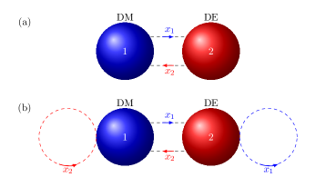
Figure 2: A new interaction schema. In (a) $x_{1}$ and $x_{2}$ denote the mutual interactions between two system, in (b) loops given dashed circles represent self-interaction of each ensemble.

By using Lemma 1, the internal energy changing in Eq.9 can be written as

$$\frac{dU_{1}}{dt}=M_{1}\Gamma_{1}x_{2},\qquad\frac{dU_{2}}{dt}=M_{2}\Gamma_{2}x_{1}$$ (10)

where $M_{1,2}$ is the mutual interaction coupling constant and $\Gamma_{1,2}$ are the the energy store velocity of the each system for the cyclic dynamic in Fig.2(b). $\Gamma_{1,2}$ are the non-holonomic variables.

Eq.(10) clearly says that the internal energy change in system 1 is determined by system 2, and conversely, the internal energy change in system 2 is determined by system 1.

On the other hand, the first term in the right hand side of Eq.(9) denote energy changing in the each system due to coupling. Therefore the heat $Q_{1,2}$ can be defined as the heat flux and it can be written as $Q_{1,2}=\phi_{1,2}=L_{1,2}x_{1,2}$. Therefore, the heat terms are given by

$$\frac{dQ_{1}}{dt}=L_{1}\frac{dx_{1}}{dt},\qquad\frac{dQ_{2}}{dt}=L_{2}\frac{dx_{2}}{dt}.$$ (11)

where $L_{1,2}$ are constants and indicate the energy store capacity of the system. Then, the second term in the right hand side of Eq.(9) can be regarded as the changing of the energy amount with time. Therefore, the second term can be written as

$$\mu_{1}\frac{dN_{1}}{dt}=\mu_{1}x_{1},\qquad\mu_{2}\frac{dN_{2}}{dt}=\mu_{2}x_{2}.$$ (12)

Finally, to simplify equations we set $L_{1}=L_{2}=1$, $\mu_{1}=\mu_{2}=1$ and $M_{1}=M_{2}=1$. If we insert Eqs.(10), (11) and (12) into Eq.(9), we can obtain interaction equations in Eq.(6) as

$$\frac{dx_{1}}{dt}=\Gamma_{1}x_{2}-x_{1}$$ (13)

$$\frac{dx_{2}}{dt}=\Gamma_{2}x_{1}-x_{2}$$ (13)

which prove Theorem 1.

Here, we introduce the mutual interaction schema for the first time and show that the mutual interaction equation between dark matter and dark energy can be obtained from the energy conservation laws of thermodynamics. However, this description in Eq.(6) is also not enough to define the interaction dynamics of two interacting and cyclic non-equilibrium systems. To obtain a completed interaction schema, non-holonomic vectorial variables $\Gamma_{1}$ and $\Gamma_{2}$ and contribution of the self-interaction loops should be defined.

Theorem 1 imply that given system in Fig.2(b) to be cyclic. The presence of cyclic interaction and the presence of vectorial non-holonomic variables $\Gamma_{1,2}$ indicate that there must be other driving vectorial forces in the system. Without these vectorial forces, it may not be possible to drive the system. At this point, we can ask the main questions: How to define the non-holonomic time-dependent degrees of freedom of the system? and What are these hidden vectorial fields? To reply to these questions and to complete the interaction description we have to deal with the role of the self-interacting loops.

III.2 Self-Interactions

Theorem 2

The non-holonomic time-dependent energy transfer rate parameters $\Gamma_{1,2}$ can be obtained hidden vectorial fields and are given in terms of $x_{1}$ and $x_{2}$ currents as

$$\frac{d\Gamma_{1}}{dt}=1-x_{1}x_{2}$$ (14a)

$$\frac{d\Gamma_{2}}{dt}=1-x_{1}x_{2}$$ (14b)

Proof: Before giving a mathematical proof, it will be useful to give the following definitions and descriptions to explain the dynamics that arise in the self-interaction scheme:

• Self-interaction loops given in Fig.2(b) represent the dynamics within systems 1 and 2.

• As seen from Fig.3, the energy $x_{1}$ flows from system 1 to system 2 and acts on system 2. Similarly, $x_{2}$ flows from the system 2 to the system 1 and acts on the system 1. While $x_{1}$ causes a rotational dynamic within the system 2, and $x_{2}$ also causes a rotational dynamic on the system 1.

• Energy flow $x_{2}$ in system 1 changes $\Gamma_{1}$ in the system 1, however, $\Gamma_{1}$ also changes the energy flow $x_{2}$. Therefore, it can be suggested that there is a non-linear relationship between these two variables. A similar situation also applies to the dynamics in system 2.

• These rotational dynamics of $x_{1,2}$ on the systems produce the non-holonomic vectorial variables which are represented by $\Gamma_{1,2}$ as seen in Fig.3.

• The rotational flow of $x_{1,2}$ on the systems will cause inertial momentum in both systems.

• Energy flow $x_{1}$ and $x_{2}$ on the systems leads to the vectorial forces $\vec{F}_{1,2}$.

• The cyclic dynamics on the loops lead to torques $\vec{\tau}_{1,2}$ we call them as vectorial attractor torques.

• The energy flows $x_{1,2}$ can be written due to the vectorial force $\vec{A}_{1,2}$ as $\vec{\nabla}\times\vec{A}_{1,2}\sim\vec{x}_{1,2}$. We call these forces as vectorial attractor fields.

• Except the energy flows $x_{1,2}$, all vector quantities occurring on the self-interaction loops and driving the systems can be regarded as virtual or pseudo quantities, we called these quantities hidden.

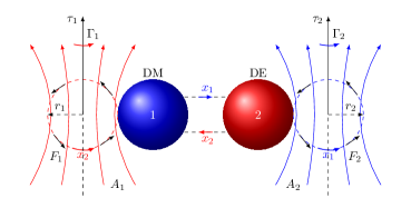
Figure 3: The vectorial attractor fields and torque behavior on the self-interacting loops. $\Gamma_{1,2}$ denotes non-holonomic variables in Eq.6. $\vec{A}_{1,2}$ are the attractor vectorial fields caused by driven force $\vec{F}_{1,2}$ and $\vec{\tau}_{1,2}$ correspond to torque on the loops.

After these definitions and descriptions, we can discuss the relation between these vectorial quantities to describe the dynamics of the self-interaction loops. It is possible to interconnect all virtual vector quantities of the self-interaction loops within the torque term.

The vectorial attractor torque can be written in terms of energy transfer velocity as

$$\vec{\tau}_{1}=c_{1}\frac{d\Gamma_{1}}{dt}\hat{z}=\vec{\tau}_{1b}+\vec{\tau}_{1f}$$ (15a)

$$\vec{\tau}_{2}=c_{2}\frac{d\Gamma_{2}}{dt}\hat{z}=\vec{\tau}_{2b}+\vec{\tau}_{2f}$$ (15b)

where $c_{1,2}$ are inertia momenta of the system 1 and 2, $\vec{\tau}_{1b,2b}$ denote torques belong to the bulk and $\vec{\tau}_{1f,2f}$ are torque cause from flux $x_{1,2}$.

The bulk torques can be assumed constant and do not contribute to the formation of the flux $x_{1,2}$, therefore, can be ignored or assigned constant values. The main torques $\vec{\tau}_{1f}$ and $\vec{\tau}_{2f}$ an the loop 1 and 2 cause form $d\vec{F}_{1}$ and $d\vec{F}_{2}$, respectively. These torques can be written in terms of vectorial fields $\vec{A}_{1}$ and $\vec{A}_{2}$ as

$$\vec{\tau}_{1f}=\int d\vec{F}_{1}\times\vec{r}_{1}=x_{1}\int\left(d\vec{r}_{1}\times\vec{A}_{1}\right)\times\vec{r}_{1}$$ (16a)

$$\vec{\tau}_{2f}=\int d\vec{F}_{2}\times\vec{r}_{2}=x_{2}\int\left(d\vec{r}_{2}\times\vec{A}_{2}\right)\times\vec{r}_{2}$$ (16b)

where loop radius $r_{1,2}$ characterize the velocity magnitude of the densities and $A_{1,2}$ are the vectorial fields on the loops. The integrals in Eq.16 can be written as

$$\int\left(d\vec{r}_{1}\times\vec{A}_{1}\right)\times\vec{r}_{1}=-M_{1}x_{2}\hat{z}$$ (17a)

$$\int\left(d\vec{r}_{2}\times\vec{A}_{2}\right)\times\vec{r}_{2}=-M_{2}x_{1}\hat{z}$$ (17b)

where $M_{1,2}$ are the positive constants. As a result, combining Eqs.15, 16 and 17, we obtain

$$c_{1}\frac{d\Gamma_{1}}{dt}=\tau_{1b}-M_{1}x_{1}x_{2}$$ (18a)

$$c_{2}\frac{d\Gamma_{2}}{dt}=\tau_{2b}-M_{2}x_{1}x_{2}$$ (18b)

Now, if we set $c_{1}=c_{2}=1$ and $\tau_{1b}=\tau_{2b}=1$, we obtain equations for non-holonomic variables $\Gamma_{1,2}$ as

$$\frac{d\Gamma_{1}}{dt}=1-x_{1}x_{2}$$ (19)

$$\frac{d\Gamma_{2}}{dt}=1-x_{1}x_{2}$$ (19)

which verify Theorem 2. Here we show that the density $x_{1}$ and $x_{2}$ behaves like current for both systems. The currents $x_{1}$ and $x_{2}$ on systems yields vectorial fields or namely the vectorial fields in this interacting schema leads $x_{1}$ and $x_{2}$ currents in the cyclic dynamics.

III.3 Full Interactions

As a result, based on Theorems 1 and  2, interaction between dark matter and dark energy is given by

$$\frac{dx_{1}}{dt}=x_{2}x_{3}-x_{1}$$

$$\frac{dx_{2}}{dt}=(x_{3}-q)x_{1}-x_{2}$$ (20)

$$\frac{dx_{3}}{dt}=1-x_{1}x_{2}$$

where $q$ is the control parameters which can be given as $q=\Gamma_{1}-\Gamma_{2}$. These are non-linear coupled equations govern the dynamics of the dark energy and dark matter interactions in Fig.1.

IV Numerical Results

To analyze the dynamical behavior of Eq.III.3, we solved these equations numerically by writing FORTRAN 90 code based on Runga-Kutta method and the linearized algorithm [44]. Phase trajectories are given in Figs.4-6.

In Fig.4, the trajectory is given in phase plane $x_{1}-x_{2}$ plane for the control parameters $q=3.46$. In this figure, there is an attractor around $x_{2}=0$ and trajectory proceeds to the right without cutting itself.

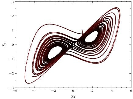
Figure 4: Chaotic attractor and trajectory in $x_{1}-x_{2}$ plane for the control parameters $q=3.46$.

In Fig.5, the attractor appears more clearly in $x_{1}-x_{3}$ plane. In this figure, it can be seen that the center of the attractor is located around $x_{3}=0$. As seen that from Fig.5 that trajectory proceeds to the right in direction $x_{1}$ without cutting itself.

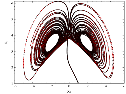
Figure 5: Chaotic attractor and trajectory in $x_{1}-x_{3}$ plane for the control parameters $q=3.46$.

In Fig.6, the trajectory is given in phase plane $x_{1}-x_{2}$ plane for the control parameters $q=3.46$ In this figure, there is an attractor around $x_{2}=0-0.5$ and and $x_{3}=1$.

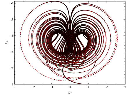
Figure 6: Chaotic attractor and trajectory in $x_{2}-x_{3}$ plane for the control parameters $q=3.46$.

We compute Lyapunov exponent by using Wolf algorithm and give the numerical results in Figs.7. As seen from Fig.7 that there are three Lyapunov exponents $\lambda_{i}$, $i=1,2,3$ for the control parameter $q$. Positive Lyapunov exponents indicate chaotic behavior of the system. One can see that two exponents (red and green curves) have positive values depend on control parameter $q$.

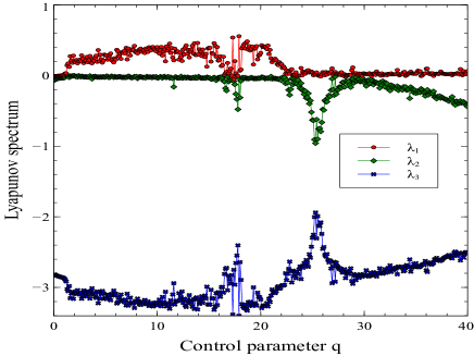
Figure 7: Lyapunov spectrum versus control parameter $q$ for the DM-DE interaction.

Lypunov spectrum in Figs.7 provides that the system in Eq.III.3 behaves as chaotic. Based on these numerical results we conclude that dark matter and dark interaction is chaotic.

In this study, it was shown for the first time that the interactions between dark matter and dark energy should be universally chaotic. These results are not only limited to dark matter and dark energy interactions but also have a universality to be generalized for all interacting particle and thermodynamic systems.

V Discussion and Some Concluding Remarks

In this study, firstly, we briefly summarized the conventional approach to the dark matter and dark energy interaction. We argued that equations of the conventional approach may not fully reflect the interaction between dark matter and dark energy, since the interaction terms are chosen arbitrarily.

We propose a new interaction schema that represents the interaction of dark matter and dark energy. We have basically demonstrated that interactions should be defined in two ways. The first is the mutual interaction between the two systems and the second is the self-interaction that occurs on each system. These two interaction pictures are beyond what has been known so far and offer a new approach to the interaction mechanisms of interacting systems. Based on the new interaction schema, we introduce new several contexts such as energy transfer velocity, vectorial attractor fields, vectorial attractor torques which are new contexts for the non-equilibrium statistical mechanics and thermodynamics. Furthermore, we introduce new theorems to define the mutual and self-interactions.

In Theorem 1, we introduce a new coupling equation to define the mutual interactions between dark matter and dark energy. We give a proof for this theorem based on the energy conservation law of thermodynamics. We also state that equations in Theorem 1 include non-holonomic variables. We know that two coupled systems out of equilibrium will exchange energy and particles until they reach fundamental and chemical equilibrium. However, the system we give in Fig.2 is not just an out-of-equilibrium coupled system. Since we assume that these systems are completely transformed into each other, the dynamics of the system are not spontaneous. The system is startled by the forces controlling the interaction dynamics. Therefore, we need to define some vectorial forces to provide the transformation of dark matter to transform into dark energy or vice versa. However, these vectorial forces drive $x_{1}$ to $x_{2}$ or $x_{2}$ to $x_{1}$ in this dynamics.

In Theorem 2, we introduce a new complementary coupling equation to define the dynamics of the non-holonomic variables. We also give a proof for Theorem 1 based on a self-interacting loop in Fig.3 motivated by the node connections approach of the graph theory.

By using these theorems, we obtain a non-linear coupling equation that fully describes dark matter and dark energy interactions. We numerically solve these equations and we obtain phase space trajectories in various phase planes. We compute Lyapunov exponents for the control parameters $q$ and show that there are non-negative values of the exponents which indicates chaos. It is the first time, based on proof-able theorems and new non-linear coupling equations, that we show that the interaction between dark matter and dark energy is fully chaotic.

Here it should be noted that, until now, in physics, it has been considered changes in thermodynamic systems in contact with each other and these changes were interpreted as interactions. However, these changes do not represent mutual interaction. It is necessary to write the interactions depending on the source. In fact, when interactions are written depending on the source, mutual interaction emerges. The basic philosophy of this study is based on this idea. In this study, the concept of mutual interaction is proposed for the first time for thermodynamic systems that come into contact with each other. As a result, the mutual interaction causes self-interaction in systems. In other words, self-interactions are the result of mutual interactions. If there are no mutual interactions, there will be no self-interaction.

It must be admitted that it is easy to visualize the mutual interaction. For example, if there is a heat $\delta Q$ transfer from one system to another, it can be assumed that heat $-\delta Q$ is transferred from the other system to the other. However, self-interaction may not be easy to understand or explain. Because no one would expect such an interaction mechanism in the classical thermodynamic system. It can be thought that since such a thing has not been expected yet, it has not been theorized. However, this counter-intuitive assumption may be understandable upon careful consideration. It should be kept in mind that if energy from one system goes to another system and causes dynamics within that system, there must be a mechanism that sets this dynamic. In this study, we propose that this mechanism can be established by the so-called forces that arise in the system. In conclusion, the interaction model we present here is quite interesting and new. Thanks to this model, it may be possible to understand the physical nature of interacting systems. Although the model seems contrary to common sense for now, however, it should not be ignored that it has the potential to add new definitions and concepts to physics.

Furthermore, one can see that these significant results can be generalized to all interacting systems such as matter and dark matter interaction visa versa. Our findings shed light on a more accurate understanding of the dynamics of the components in the universe. Furthermore, these results strongly prove that the universe has chaotic dynamics. In the previous study [38], we proposed that interactions between matter, dark matter, and dark energy would be chaotic. At the same time, we stated that the universe evolves through chaotic interactions and that the universe has cosmic evolution with chaotic cyclical processes. In this study, we have strongly proved these hypotheses in a new theoretical framework.

This theoretical evidence not only explains the interaction of dark matter and dark energy but also reveals an important and striking perspective in terms of understanding how nature works. The interaction equations we have obtained have provided a completely new understanding of nature by illuminating the hitherto unnoticed behavior of interacting systems in nature.

It is very important to mention another crucial point. The interaction scheme in Fig.3, Theorem 1, Theorem 2 and interaction equations in (III.3 and all the results we obtained here are valid not only for cosmology but also for all coupled non-equilibrium thermodynamic systems. The results also show that the dynamics of all coupled, interacting, and transforming thermodynamic systems are chaotic at far from equilibrium and near the equilibrium. This is also another significant result of the present study. Additionally, these results may indicate the presence of new thermodynamics laws.

If we sum up, in this study, we theoretically show that the interacting coupling thermodynamic systems behave as chaotic. It is clear that these theoretical findings will have important contributions to physics. It is possible for these theoretical discoveries to be proven experimentally, and it is clear that experimental studies will confirm the theoretical discoveries.

Finally, we conclude that this result can be generalized to the $N$ coupling systems which behave as interaction networks. In addition to the chaotic behavior of all elements in such an interaction network, the complex system itself is expected to behave chaotically. The human neural network, which is a self-organized system, can be the best example of this. We know that chaos characterizes the dynamics of a system whose dynamics are sensitive to the initial conditions and whose time evolution is unpredictable. However, at this point, we can give a new definition of chaos: Chaos is the collective minimum action of the synchronized self-organized interacting systems.

VI Summary of the Main Results

1. Interaction between dark matter and dark energy: The interaction between dark matter and dark energy is chaotic.

2. Hidden Symmetry: All coupled interacting particle and thermodynamic systems have hidden symmetries that can be represented by the self-interaction loops.

3. Hidden Interaction: The self-interaction loops of the coupled interacting particle and thermodynamic systems have hidden variables and vectorial fields.

4. New Physics Law: The dynamics of all coupled interacting particle and thermodynamic systems are chaotic.

5. Definition of the Chaos: Chaos is the minimum action of the coupled, synchronized, self-organized interacting systems.

6. Self-organization: All self-organized systems are the manifestation of chaotic behavior.

References

- Rubin and Ford [1970] V. C. Rubin and J. Ford, W. Kent, Astrophys. J. 159, 379 (1970).
- Rubin et al. [1980] V. C. Rubin, J. Ford, W. K., and N. Thonnard, Astrophys. J. 238, 471 (1980).
- Trimble [1987] V. Trimble, Annual Review of Astronomy and Astrophysics 25, 425 (1987), https://doi.org/10.1146/annurev.aa.25.090187.002233 .
- Riess et al. [1998] A. G. Riess, A. V. Filippenko, P. Challis, A. Clocchiatti, A. Diercks, P. M. Garnavich, R. L. Gilliland, C. J. Hogan, S. Jha, R. P. Kirshner, B. Leibundgut, M. M. Phillips, D. Reiss, B. P. Schmidt, R. A. Schommer, R. C. Smith, J. Spyromilio, C. Stubbs, N. B. Suntzeff, and J. Tonry, The Astronomical Journal 116, 1009 (1998), astro-ph/9805201 .
- Perlmutter et al. [1999] S. Perlmutter, G. Aldering, G. Goldhaber, R. A. Knop, P. Nugent, P. G. Castro, S. Deustua, S. Fabbro, A. Goobar, D. E. Groom, I. M. Hook, A. G. Kim, M. Y. Kim, J. C. Lee, N. J. Nunes, R. Pain, C. R. Pennypacker, R. Quimby, C. Lidman, R. S. Ellis, M. Irwin, R. G. McMahon, P. Ruiz-Lapuente, N. Walton, B. Schaefer, B. J. Boyle, A. V. Filippenko, T. Matheson, A. S. Fruchter, N. Panagia, H. J. M. Newberg, W. J. Couch, and T. S. C. Project, The Astrophysical Journal 517, 565 (1999).
- Bennett et al. [2013] C. L. Bennett, D. Larson, J. L. Weiland, N. Jarosik, G. Hinshaw, N. Odegard, K. M. Smith, R. S. Hill, B. Gold, M. Halpern, E. Komatsu, M. R. Nolta, L. Page, D. N. Spergel, E. Wollack, J. Dunkley, A. Kogut, M. Limon, S. S. Meyer, G. S. Tucker, and E. L. Wright, The Astrophysical Journal Supplement Series 208, 20 (2013).
- Hinshaw et al. [2013] G. Hinshaw, D. Larson, E. Komatsu, D. N. Spergel, C. L. Bennett, J. Dunkley, M. R. Nolta, M. Halpern, R. S. Hill, N. Odegard, L. Page, K. M. Smith, J. L. Weiland, B. Gold, N. Jarosik, A. Kogut, M. Limon, S. S. Meyer, G. S. Tucker, E. Wollack, and E. L. Wright, The Astrophysical Journal Supplement Series 208, 19 (2013).
- Planck Collaboration et al. [2020] Planck Collaboration, Aghanim, N., Akrami, Y., Ashdown, M., Aumont, J., Baccigalupi, C., Ballardini, M., Banday, A. J., Barreiro, R. B., Bartolo, N., Basak, S., Battye, R., Benabed, K., Bernard, J.-P., Bersanelli, M., Bielewicz, P., Bock, J. J., Bond, J. R., Borrill, J., Bouchet, F. R., Boulanger, F., Bucher, M., Burigana, C., Butler, R. C., Calabrese, E., Cardoso, J.-F., Carron, J., Challinor, A., Chiang, H. C., Chluba, J., Colombo, L. P. L., Combet, C., Contreras, D., Crill, B. P., Cuttaia, F., de Bernardis, P., de Zotti, G., Delabrouille, J., Delouis, J.-M., Di Valentino, E., Diego, J. M., Doré, O., Douspis, M., Ducout, A., Dupac, X., Dusini, S., Efstathiou, G., Elsner, F., Enßlin, T. A., Eriksen, H. K., Fantaye, Y., Farhang, M., Fergusson, J., Fernandez-Cobos, R., Finelli, F., Forastieri, F., Frailis, M., Fraisse, A. A., Franceschi, E., Frolov, A., Galeotta, S., Galli, S., Ganga, K., Génova-Santos, R. T., Gerbino, M., Ghosh, T., González-Nuevo, J., Górski, K. M., Gratton, S., Gruppuso, A., Gudmundsson, J. E., Hamann, J., Handley, W., Hansen, F. K., Herranz, D., Hildebrandt, S. R., Hivon, E., Huang, Z., Jaffe, A. H., Jones, W. C., Karakci, A., Keihänen, E., Keskitalo, R., Kiiveri, K., Kim, J., Kisner, T. S., Knox, L., Krachmalnicoff, N., Kunz, M., Kurki-Suonio, H., Lagache, G., Lamarre, J.-M., Lasenby, A., Lattanzi, M., Lawrence, C. R., Le Jeune, M., Lemos, P., Lesgourgues, J., Levrier, F., Lewis, A., Liguori, M., Lilje, P. B., Lilley, M., Lindholm, V., López-Caniego, M., Lubin, P. M., Ma, Y.-Z., Macías-Pérez, J. F., Maggio, G., Maino, D., Mandolesi, N., Mangilli, A., Marcos-Caballero, A., Maris, M., Martin, P. G., Martinelli, M., Martínez-González, E., Matarrese, S., Mauri, N., McEwen, J. D., Meinhold, P. R., Melchiorri, A., Mennella, A., Migliaccio, M., Millea, M., Mitra, S., Miville-Deschênes, M.-A., Molinari, D., Montier, L., Morgante, G., Moss, A., Natoli, P., Nørgaard-Nielsen, H. U., Pagano, L., Paoletti, D., Partridge, B., Patanchon, G., Peiris, H. V., Perrotta, F., Pettorino, V., Piacentini, F., Polastri, L., Polenta, G., Puget, J.-L., Rachen, J. P., Reinecke, M., Remazeilles, M., Renzi, A., Rocha, G., Rosset, C., Roudier, G., Rubiño-Martín, J. A., Ruiz-Granados, B., Salvati, L., Sandri, M., Savelainen, M., Scott, D., Shellard, E. P. S., Sirignano, C., Sirri, G., Spencer, L. D., Sunyaev, R., Suur-Uski, A.-S., Tauber, J. A., Tavagnacco, D., Tenti, M., Toffolatti, L., Tomasi, M., Trombetti, T., Valenziano, L., Valiviita, J., Van Tent, B., Vibert, L., Vielva, P., Villa, F., Vittorio, N., Wandelt, B. D., Wehus, I. K., White, M., White, S. D. M., Zacchei, A., and Zonca, A., A&A 641, A6 (2020).
- Fitch et al. [1998] V. L. Fitch, D. R. Marlow, M. A. E. Dementi, and F. J. Dyson, American Journal of Physics 66, 837 (1998), https://doi.org/10.1119/1.18973 .
- Zlatev et al. [1999] I. Zlatev, L. Wang, and P. J. Steinhardt, Physical Review Letters 82, 896 (1999).
- del Campo et al. [2006] S. del Campo, R. Herrera, G. Olivares, and D. Pavón, Phys. Rev. D 74, 023501 (2006).
- He et al. [2011] J.-H. He, B. Wang, and E. Abdalla, Phys. Rev. D 83, 063515 (2011).
- Poitras [2014] V. Poitras, Gen Relativ Gravit. 46, 1732 (2014).
- Brax and Martin [2006] P. Brax and J. Martin, Journal of Cosmology and Astroparticle Physics 11, 008, arXiv:astro-ph/0606306 .
- Bolotin et al. [2015] Y. L. Bolotin, A. Kostenko, O. Lemets, and D. Yerokhin, International Journal of Modern Physics D 24, 1530007 (2015), arXiv:1310.0085 [astro-ph.CO] .
- Zimdahl and Pavon [2004] W. Zimdahl and D. Pavon, General Relativity and Gravitation 36, 1483–1491 (2004), arXiv:gr-qc/0311067 .
- Amendola et al. [2007] L. Amendola, G. C. Campos, and R. Rosenfeld, Phys. Rev. D 75, 083506 (2007), arXiv:astro-ph/0610806 .
- Wang et al. [2016] B. Wang, E. Abdalla, F. Atrio-Barandela, and D. Pavon, Reports on Progress in Physics 79, 096901 (2016), arXiv:1603.08299 [astro-ph.CO] .
- Böhmer et al. [2015a] C. G. Böhmer, N. Tamanini, and M. Wright, Phys. Rev. D 91, 123002 (2015a), arXiv:1501.06540 [gr-qc] .
- Böhmer et al. [2015b] C. G. Böhmer, N. Tamanini, and M. Wright, Phys. Rev. D 91, 123003 (2015b), arXiv:1502.04030 [gr-qc] .
- He and Wang [2008] J.-H. He and B. Wang, Journal of Cosmology and Astroparticle Physics 06, 010, arXiv:70801.4233 [astro-ph] .
- Cai et al. [2017] R.-G. Cai, N. Tamanini, and T. Yang, Journal of Cosmology and Astroparticle Physics 05, 031, arXiv:1703.07323 [astro-ph.CO] .
- Yang et al. [2019] W. Yang, N. Banerjee, A. Paliathanasis, and S. Pan, Physics of the Dark Universe 26, 100383 (2019), arXiv:1812.06854 [astro-ph.CO] .
- Amendola [2000] L. Amendola, Phys. Rev. D 62, 043511 (2000), arXiv:astro-ph/9908023 .
- Tocchini-Valentini and Amendola [2002] D. Tocchini-Valentini and L. Amendola, Phys. Rev. D 65, 063508 (2002), arXiv:astro-ph/0108143 .
- Amendola and Quercellini [2003] L. Amendola and C. Quercellini, Phys. Rev. D 68, 023514 (2003), arXiv:astro-ph/0303228 .
- del Campo et al. [2008] S. del Campo, R. Herrera, and D. Pavon, Phys. Rev. D 78, 021302 (2008), arXiv:0806.2116 [astro-ph] .
- del Campo et al. [2009] S. del Campo, R. Herrera, and D. Pavon, Journal of Cosmology and Astroparticle Physics (01), 020, arXiv:0812.2210 [gr-qc] .
- Wei and Zhang [2007] H. Wei and S. N. Zhang, Physics Letters B 644, 7 (2007), arXiv:astro-ph/0609597 .
- del Campo et al. [2015] S. del Campo, R. Herrera, and D. Pavón, Phys. Rev. D 91, 123539 (2015), arXiv:1507.00187 [gr-qc] .
- Chimento [2010] L. P. Chimento, Phys. Rev. D 81, 043525 (2010), arXiv:0911.5687 [astro-ph.CO] .
- Sanchez and Ivan [2014] G. Sanchez and E. Ivan, Gen. Rel. Grav. 46, 1769 (2014), arXiv:1405.1291 [gr-qc] .
- Verma [2010] M. M. Verma, Astrophys Space Sci 330, 101 (2010).
- Shahalam et al. [2015] M. Shahalam, S. D. Pathak, M. M. Verma, M. Y. Khlopov, and R. Myrzakulov, Eur. Phys. J. C 75, 395 (2015), arXiv:1503.08712 [gr-qc] .
- Cruz and Lepe [2018] M. Cruz and S. Lepe, Classical and Quantum Gravity 35, 155013 (2018).
- Cruz et al. [2019] M. Cruz, S. Lepe, and G. Morales-Navarrete, Nuclear Physics B 943, 114623 (2019).
- Saleem and Imtiaz [2020] R. Saleem and M. J. Imtiaz, Classical and Quantum Gravity 37, 065018 (2020).
- Aydiner [2018] E. Aydiner, Scientific Reports 8, 721 (2018).
- Aydiner et al. [2022] E. Aydiner, I. Basaran-Öz, T. Dereli, and M. Sarisaman, Eur. Phys. J. C 82, 39 (2022).
- Arneodo et al. [1980] A. Arneodo, P. Coullet, and C. Tresser, Physics Letters A 79, 259 (1980).
- Vano et al. [2006] J. A. Vano, J. C. Wildenberg, M. B. Anderson, J. K. Noel, and J. C. Sprott, Nonlinearity 19, 2391 (2006).
- Perez et al. [2014] J. Perez, A. Füzfa, T. Carletti, L. Mélot, and L. Guedezounme, General Relativity and Gravitation 46, 10.1007/s10714-014-1753-8 (2014).
- Prigogine et al. [1988] I. Prigogine, J. Geheniau, E. Gunzig, and P. Nardone, Proceedings of the National Academy of Sciences 85, 7428 (1988), https://www.pnas.org/doi/pdf/10.1073/pnas.85.20.7428 .
- Wolf et al. [1985] A. Wolf, J. B. Swift, H. L. Swinney, and J. A. Vastano, Physica D: Nonlinear Phenomena 16, 285 (1985).