Luciano Pandolfi

The Lebesgue Integral
Via The Tonelli Method

Preface

The theory of Lebesgue integration was developed by H.-L. Lebesgue in his doctoral dissertation published in 1902 in the italian Journal Annali di Matematica Pura ed Applicata (see [17]). The theory of Lebesgue integration was soon fully appreciated by the leading mathematicians in Italy, also thanks to the activity of Vitali, and important results soon proved: Fubini Theorem was proved in 1907 (in [11]). Leonida Tonelli first used Lebesgue integral in 1908, in [37], while studying rectifiable curves.

As soon as the importance of Lebesgue integration was recognized, different approaches were proposed both to put the theory in a more general framework, as in [5], and also in order to speed up the presentation of the crucial ideas. In fact, for didactic reasons, several authors tried to bypass or reduce to a minimum the preliminary study of the measure of sets and to lead students to appreciate the key ideas of Lebesgue integration in the shortest possible time. Among these approaches, the one which is likely the most well known is due to F. Riesz. This approach is the one used in [30] and recently simplified in [16]. Instead, the Daniell’s approach, introduced in [5], intends to be more general and abstract.

Leonida Tonelli devised an efficient approach to Lebesgue integration, based on the notion of “quasicontinuous functions”, which requires only a basic knowledge of calculus together with a certain level of mathematical ingenuity.

Quasicontinuous functions are precisely the functions which are measurable according to Lebesgue, but defined in terms of elementary continuity properties.

It seems to me that this approach proposed by Tonelli, and which is virtually unknown to young people, has its merits since most of the methods used to construct the Lebesgue integral hide the real reasons for the introduction of a new kind of integral. We cite from [30, p. 29]: “The reason for such a change [the shift from Riemann to Lebesgue integration] and, with them, the usefulness and beauty of the Lebesgue theory, will be seen in the course of the following chapters; there is no point in speaking of them in advance”. Instead, the reason is clearly displayed in the Tonelli approach, since it constitutes the foundation over which the integral is constructed.

Lebesgue integral is introduced by exploiting the method of Tonelli in [4] (for functions of one variable. [4, Chap. VI] concisely defines the integral for functions of two variables and proves Fubini theorem), and in part in the book [29]. As stated by the authors, the first version of this book was prepeared for the lessons given by Picone when he gave the course of Tonelli, after Tonelli’s death. Few books, as [15, 32], present a sketch of Tonelli ideas.

For this reason we give here a quite complete account of Tonelli method.

We divide the presentation in three parts: in the first part we study integration in the simpler case of the functions of one variable. The fundamental notion that the student has to master is that of “quasicontinuous function”. Once this is done, Lebesgue integral appears as a straightforward extension of Riemann integral thanks to an “exchange of limits and integrals” which is precisely the goal for which the new integral has been introduced.

This chapter ends with the statement of the theorems of the exchange of the limits and the integral, with a sketch of a proof. The details of the proofs are in Chap. 2.

The first chapter can be used as an efficient introduction to the Lebesgue integration even in courses for mathematically motivated engineering students, for example as a preliminary to a basic course on Hilbert spaces.

The second part extends the arguments of the first part to functions of several variables (in the Chapters 3 and 4). Chap. 5 is devoted to Fubini Theorem on the reduction of multiple integrals.

For the sake of completeness, the third part, containing the sole Chap. 6, shows the well known fact that once the integral has been defined then Lebesgue and Borel measurable sets can be defined and the properties of the measure can be obtained from those of the integral.

Finally we repeat that the usual presentation of Lebesgue integration proceeds from the study of the measure and measurable sets to the theory of measurable functions and then to the theory of the integral. This way the students have to study first abstract measure theory which has its independent importance, for example for the application to probability. Instead, in the Tonelli approach measure theory is derived as a byproduct of the study of the integral and the abstract measure theory remains in the shadow. This fact, which can be seen as an important limitation now, was instead the goal of Tonelli and others. For example, Tonelli states in the introduction of his 1924 paper [38]: “this paper is an attempt to put on a simple, let us say elementary, and so more acceptable, basis the theory of Lebesgue integration by removing measure theory at all”. Similar approaches to a direct introduction of the integrals done in the same period state explicitly the same goals. Beppo Levi introduced his own approach to Lebesgue integration in the same year 1924 and in the same journal as Tonelli did and for similar reasons (see [23]): “It is a fact that in front of the importance of the new theory [i.e. the Lebesgue theory] there are obvious didactic and logical difficulties…due also to the need of a preliminary study of the theory of the measure of sets”. The introduction of F. Riesz and B. Sz-Nagy book [30] states “The two parts [of the book] form an organic unity centered about the concept of linear operator. This concept is reflected in the method by which we have constructed the Lebesgue integral; this method, which seems to us to be simpler and clearer then that based on the theory of measure…”

Finally we mention that Picone too proposed his approach to the Lebesgue integration for functions of Baire classes (see for example [28]), by a repeated use of limiting processes.

We conclude this introduction with a warning. The development of Lebesgue integration was stimulated by two main difficulties encountered with Riemann integration:

1. the fact that the pointwise limit of a sequence of continuous functions may not be Riemann integrable, a fact soon realized after that a rigorous definition of the integral (and also of the concept of function) had been given. A consequence is that limits and Riemann integrals cannot be exchanged in the generality needed to study for example Fourier series (and Riemann integral cannot be used to define Hilbert spaces).

2. the existence of derivative functions which are not Riemann integrable, a fact discovered by V. Volterra in 1881, see [46].

In our exposition we concentrate on the first problem, the problem of exchanging limits and integrals. The second problem, of recovering a function from its derivative, will not be considered here. Readers interested in the relation of the integral and the derivative can see for example [1] or, for an approach based on Daniell ideas, [34].

People interested in the origin and the history of the Lebesgue integration can look at the book [14] and to the expositions [20, 21] made by Lebesgue himself.

Contents

1. Preface
2. I Functions of One Variable
   1. 1 The Lebesgue Integral for Functions of One Variable
      1. 1.1 The Limitations of the Riemann Integral
      2. 1.2 Subsets of the Real Line and Continuity
         1. 1.2.1 Restriction and Extensions of Functions
            1. Associated Multiintervals
         2. 1.2.2 Tietze Extension Theorem: One Variable
      3. 1.3 Tonelli Construction of the Lebesgue Integral
         1. 1.3.1 The Key Ingredients Used by Tonelli
            1. The Properties of the Quasicontinuous Functions
         2. 1.3.2 The Lebesgue Integral under Boundedness Assumptions
         3. 1.3.3 Unbounded Functions and Domains
            1. Lebesgue Integral and Improper Integral
      4. 1.4 Limits and the Integral
      5. 1.5 Appendix: Riemann and Lebesgue Integrals
         1. 1.5.1 A Sketch of the Riemann Integral
            1. The Oscillation of a Function
            2. Riemann Integral: the Conditions of Integrability
            3. Riemann Integrability and Continuity
         2. 1.5.2 Riemann and Lebesgue Integrability
   2. 2 Limits and Integrals: One Variable
      1. 2.1 Egorov-Severini Theorem and Quasicontinuity
         1. 2.1.1 Consequences of the Egorov-Severini Theorem
         2. 2.1.2 Absolute Continuity of the Integral
      2. 2.2 The Limit of Sequences and the Lebesgue Integral
         1. 2.2.1 Bounded Sequences on a Bounded Interval
         2. 2.2.2 Sequences of Nonnegative Functions
         3. 2.2.3 The General Case: Lebesgue Theorem
      3. 2.3 Appendix: Egorov-Severini: Preliminaries in One Variable
         1. 2.3.1 Convergent and Uniformly Convergent Sequences
         2. 2.3.2 The Two Main Lemmas
         3. 2.3.3 From Lemma 102 to Theorem 82:
3. II Functions of Several Variables
   1. 3 Functions of Several Variables: the Integral
      1. 3.1 Rectangles, Multirectangles and Null Sets
      2. 3.2 The Tietze Extension Theorem: Several Variables
      3. 3.3 The Lebesgue Integral in $\mathbb{R}^{d}$
         1. 3.3.1 The Properties of the Integral
      4. 3.4 Appendix: Tonelli and the Tietze Extension
         1. 3.4.1 Few Notations
         2. 3.4.2 The Proof of Theorem 113
   2. 4 The Limits and the Integral
      1. 4.1 Special Classes of Sets and Multirectangles
         1. 4.1.1 Almost Disjoint Multirectangles and their Measure
         2. 4.1.2 Representation of Nonempty Open Sets
      2. 4.2 Egorov-Severini Theorem and Quasicontinuity
      3. 4.3 Absolute Continuity of the Integral
         1. 4.3.1 The Characteristic Function of an Open Set
         2. 4.3.2 Absolute Continuity: the Proof of Theorem 151
      4. 4.4 The Limit of Sequences and the Lebesgue Integral
      5. 4.5 Appendix: Egorov-Severini: Preliminaries in Several Variables
         1. 4.5.1 Preliminary Observations
         2. 4.5.2 The Proof of Theorem 147
   3. 5 Reduction of Multiple Integrals
      1. 5.1 Discussion and the Reduction Formulas
         1. 5.1.1 Notations and the Statements of the Theorems
         2. 5.1.2 Preliminary Results
            1. Observation on Null Sets and Quasicontinuous Functions
            2. Sections of Multirectangle Sets
      2. 5.2 Fubini and Tonelli Theorems: the Proofs
         1. Fubini Theorem: $f$ Bounded on a Bounded Rectangle
            1. Fubini Theorem under General Assumptions
               1. Tonelli Theorem: the Proof
4. III Recovering Lebesgue Measure
   1. 6 Borel and Lebesgue Measure
      1. 6.1 Open Sets and Lebesgue Measurable Sets
         1. 6.1.1 The Measure of Lebesgue Measurable Sets
         2. 6.1.2 Absolute Continuity of the Integral: the General Case
      2. 6.2 Borel Sets and Lebesgue Sets
         1. 6.2.1 Multirectangle Sets and Lebesgue Measurable Sets
      3. 6.3 Littlewood’s Three Principles
      4. 6.4 Lebesgue Definition of Measurable Sets
      5. 6.5 Appendix: A Set Which is not Lebesgue Measurable
      6. 6.6 A Null Set Which is not Borel Measurable

Part I Functions of One Variable

Chapter 1 The Lebesgue Integral for Functions of One Variable

This chapter is intended for general students af science and engineering with possibly just calculus courses but a sufficient motivation. In particular, we assume familiarity with Riemann integration whose key points are recalled in the Appendix 1.5.1.

This chapter can be used as the introductory chapter of a course on Hilbert spaces. For this reason first we describe the limitations of the Riemann integral and then we use Tonelli method as an efficient tool to introduce the key ideas of the Lebesgue integration.

At the end of this chapter we state and shortly illustrate the theorems on the exchange of limits and integrals. The details of the proofs are in Chap. 2.

Our goal here is the presentation of key ideas and for this reason we confine ourselves to consider functions of one variable. The general case of functions of several variables is in Part II.

1.1 The Limitations of the Riemann Integral

When presenting the definition of the Riemann integral, usually instructors show the existence of functions which are not Riemann integrable. The standard example is the Diriclet function on $[0,1]$:

$$d(x)=\left\{\begin{array}[]{lll}1&{\rm if}&x\in\mathbb{Q}\\ 0&{\rm if}&x\in\mathbb{R}\setminus\mathbb{Q}\,.\end{array}\right.$$ (1.1)

It is easily seen that this function is not Riemann integrable and it is often asserted that examples like this one prompt for the definition of a more general kind of integral.

We may ask ourselves whether there is any reason to integrate such kind of pathological functions. At first glance it seems that there is no reason at all. But, let us look at the problem from a different point of view.

Even the first elements of calculus make an essential use of the notion of limits and continuity. A function $f$ is continuous at $x_{0}\in{\rm dom}\,f$ when for every sequence $\{x_{n}\}$ with $x_{n}\in{\rm dom}\,f$ and such that $x_{n}\to x_{0}$ we have

$$\lim f(x_{n})=f(x_{0})=f\left(\lim x_{n}\right)\,.$$

Continuity is the property that the limit and the function can be exchanged.

Now we observe that Riemann integral is a function which associates a number to a set of functions. So, we introduce:

Definition 1

1. Let $\mathcal{D}$ be a set of functions. We call functional a transformation which associates a number to any element of $\mathcal{D}$.

2. Let it be possible to define the limit of sequences in $\mathcal{D}$ and let $\mathcal{F}$ be a functional defined on $\mathcal{D}$. We say that $\mathcal{F}$ is continuous at $f_{0}\in\mathcal{D}$ when the following holds for every sequence $\{f_{n}\}$ in $\mathcal{D}$, $f_{n}\to f_{0}$:

   $$\lim\mathcal{F}(f_{n})=\mathcal{F}\left(\lim f_{n}\right)\,.$$

Riemann integral is a functional on $\mathcal{D}=C([h,k])$ (for every bounded interval $[h,k]$) and it is possible to define the limits of sequences in $C([h,k])$ as follows: the sequence $\{f_{n}\}$ converges to $f$ uniformly on $[h,k]$ when the following holds:

$$\forall\varepsilon>0\ \exists N_{\varepsilon}\ \mbox{such that}\ n>N_{\varepsilon}\ \implies\ -\varepsilon<f_{n}(x)-f(x)<\varepsilon\quad\forall x\in[h,k]\,.$$ (1.2)

I.e. we require that for $n>N_{\varepsilon}$ we have

$$-\varepsilon<\inf_{[h,k]}(f_{n}-f)\leq\sup_{[h,k]}(f_{n}-f)<\varepsilon\,.$$

So we have the following result:

Theorem 2

The sequence $\{f_{n}\}$ is uniformly convergent to $f$ if and only if we have

$$\lim_{n\to+\infty}\inf_{[h,k]}(f_{n}-f)=0\quad\mbox{and}\quad\lim_{n\to+\infty}\sup_{[h,k]}(f_{n}-f)=0\,.$$

From a graphical point of view, uniform convergence is the property that for large $n$ the graphs of $f_{n}$ stay in a “tube” of width $\varepsilon$ around that of $f$, as in the figure on the right.

It turns out that Riemann integral as a functional on $C([h,k])$ is continuous:

Theorem 3

Let $[h,k]$ be a bounded interval and let $\{f_{n}\}$ be a uniformly convergence sequence in $C([h,k])$. Then:

$$\lim_{n\to+\infty}\int_{h}^{k}{f_{n}(x)}\;\mbox{\rm d}x=\int_{h}^{k}\left(\lim_{n\to+\infty}f_{n}(x)\right)\;\mbox{\rm d}x\,.$$ (1.3)

Now we observe:

• Riemann integral is defined on a set of functions which is larger then $C([h,k])$. In particular, any piecewise continuous function is Riemann integrable.

• Uniform convergence is a very strong property. Much too strong for most of the applications of mathematics. As an example, let us consider the following important equality:

  $$\lim_{n\to+\infty}\left[\sum_{k=1}^{n}\frac{1}{k}\sin kx\right]=\chi(x)$$ (1.4)

  where $\chi(x)$ is the extension of period $2\pi$ of the odd extension to $(-\pi,0)$ of

  $$[(\pi-x)/2]\quad 0<x<\pi$$

  (see the graph on the right). The sequence of the functions

  $$f_{n}(x)=\sum_{k=1}^{n}\frac{1}{k}\sin kx$$

  is a sequence of continuous functions while $\chi$ has jumps.

  

It is known that the uniform limit of a sequence of continuous functions is continuous and so the limit in (1.4) cannot be uniform in an interval which contains jumps of $\chi$. On these intervals Theorem 3 cannot be applied.

The equality (1.4) is a simple example of a Fourier series and it is seen in every elementary introduction to the Fourier series that a key point in the justification of the equality (1.4) is the exchange of the series (i.e. of a limit) with suitable integrals. So, in order to justify (1.4) we must use an analogous of Theorem 3 when the limit exists but the convergence is not uniform. Unfortunately, the following example shows that if the convergence is not uniform in general the limit and the Riemann integral cannot be exchanged.

Example 4

The sole condition that each $f_{n}$ is Riemann integrable and that $\{f_{n}(x)\}$ converges to $f(x)$ for every $x\in[h,k]$ does not imply the equality (1.3). This can be seen as follows. We recall the following property: a bounded function which is equal $0$ a part finitely many points is Riemann integrable and its integral is $0$.

It is known that the rationals in $[0,1]$ constitute a numerable set, i.e. they can be arranged to be the image of a sequence $\{q_{n}\}$.

For every $n$ we define

$$f_{n}(x)=\left\{\begin{array}[]{lll}1&{\rm if}&\mbox{$x=q_{k}$ with $k\leq n$}\\ 0&&\mbox{otherwise}\,.\end{array}\right.$$ (1.5)

Each function $f_{n}$ differs from $0$ in $n$ points and so $f_{n}$ is integrable with integral equal $0$. The equality (1.3) does not hold since for every $x$ we have $f_{n}(x)\to d(x)$, the Dirichlet function, and $d(x)$ is not Riemann integrable.   

This example however is not entirely satisfactory since we can wonder whether there is any concrete interest in the functions $f_{n}$ just constructed. So, let us see a second example.

Example 5

We consider functions defined on $[0,1]$ and a limiting process in two steps. Let us fix a natural number $m$ and let us consider the sequence of the continuous functions

$$n\mapsto\left[\cos(m!)\pi x\right]^{2n}\,.$$

Then we define the function

$$\phi_{m}(x)=\lim_{n\to+\infty}\left[\cos(m!)\pi x\right]^{2n}\,.$$

If $x\notin\mathbb{Q}$ then $|\cos(m!)\pi x|<1$ and so

$$x\notin\mathbb{Q}\ \implies\ \phi_{m}(x)=0\,.$$

Let instead $x\in\mathbb{Q}$, $x=p/q$ with $p<q$. We have

$$\begin{array}[]{l}\cos(m!)\pi x=\cos\dfrac{pm!}{q}\pi=\pm 1\quad\mbox{if $q$ divides $pm!$}\\ |\cos(m!)\pi x|<1\quad\mbox{otherwise}\,.\end{array}$$

For a fixed value of $m$, the denominator $q$ divides $pm!$ only for finitely rational number $p/q\in[0,1]$ and so

$$\phi_{m}(x)=1\ \mbox{for finitely many values of $x\in[0,1]$; otherwise $\phi_{m}(x)=0$}\,.$$

Hence $\phi_{m}$ is Riemann integrable and its integral is equal zero.

Now we consider

$$\lim_{m\to+\infty}\phi_{m}(x)\,.$$

If $x\notin\mathbb{Q}$ then the limit is zero since $\phi_{m}(x)=0$ for every $m$.

Let $x=p/q$. When $m$ is sufficient large, say $m>2q$, the number $(m!)p/q$ is an even number and $\phi_{m}(x)=1$.

It follows that $\lim_{m\to+\infty}\phi_{m}(p/q)=1$. Hence

$$\lim_{m\to+\infty}\phi_{m}(x)=d(x)$$

a non integrable function.

In conclusion, we are in the same situation as in the Example 4: limit and integral cannot be exchanged. But now we have an example which is significant since it shows that the Dirichlet function can be obtained by computing limits of cosine functions; and sequences of sine and cosine functions are the basis of the Fourier analysis, a crucial tool in every application of mathematics.   

In fact, from the historical point of view it was Fourier analysis that stimulated the introduction of several variants of the Riemann integral in the course of the XIX century. This process then culminated in 1902 with the introduction of the Lebesgue integral in [17].

Remark 6

We repeat again: the desired equality (1.3) is the reason for the construction of an integral which can integrate such patological functions like the Dirichlet function, and not the interest of such functions by themselves.

Note that Example 5 contains also a second piece of information: if equality (1.3) has to hold then the Dirichlet function not only has to be integrable but its integral has to be zero.   

Now we sum up our rather optimistic dream: we would like a new kind of integral for which the following properties hold:

1. if $f(x)\equiv c$ on $[h,k]$ then it is integrable and its integral is $c(k-h)$ i.e. the area of the rectangle identified by its graph;

2. additivity of the integral: if $f(x)$ is defined on $A\cup B$ and it is integrable both on $A$ and on $B$ then it is integrable on its domain $A\cup B$. Moreover we want:

   $$A\cap B=\emptyset\ \implies\ \int_{A\cup B}f(x)\;\mbox{\rm d}x=\int_{A}f(x)\;\mbox{\rm d}x+\int_{B}f(x)\;\mbox{\rm d}x\,.$$

   In concrete terms, if $A=[h,\tilde{h})$ and $B=[\tilde{h},k]$ we want

   $$\int_{h}^{k}f(x)\;\mbox{\rm d}x=\int_{h}^{\tilde{h}}f(x)\;\mbox{\rm d}x+\int_{\tilde{h}}^{k}f(x)\;\mbox{\rm d}x\,.$$

3. let $\{f_{n}\}$ be a sequence of integrable functions on a set $A$ and let $\lim f_{n}(x)=f(x)$ for every $x\in A$. Then we wish that $f$ be integrable too and

   $$\lim_{n\to+\infty}\int_{A}f_{n}(x)\;\mbox{\rm d}x=\int_{A}\left(\lim_{n\to+\infty}f_{n}(x)\right)\;\mbox{\rm d}x\,.$$ (1.6)

The following examples show that these requirements are contradictory and cannot be achieved.

Example 7

Let $f_{n}$ be defined on $[0,1]$ as follows:

$$f_{n}(x)=\left\{\begin{array}[]{lll}0&{\rm if}&0\leq x\leq 1/n\\ n&{\rm if}&1/n<x\leq 2/n\\ 0&{\rm if}&2/n\leq x\leq 1\,.\end{array}\right.$$

It is clear that

$$\mbox{$\lim f_{n}(x)=0=f(x)$ per ogni $x\in[0,1]$}\,.$$

The first and second requirements show that the functions $f_{n}$ and $f$ are integrable and give the value of the integrals:

$$0=\int_{0}^{1}f(x)\;\mbox{\rm d}x\neq\lim_{n\to+\infty}\underbrace{\int_{0}^{1}f_{n}(x)\;\mbox{\rm d}x}_{=1\ \mbox{for every $n$}}=1\,.$$

A similar example can be given for integrals on unbounded domains. Let the domain be $[0,+\infty)$. In this case we define

$$f_{n}(x)=\left\{\begin{array}[]{lll}0&{\rm if}&x\leq n\\ 1/n&{\rm if}&n<x\leq 2n\\ 0&{\rm if}&x>2n\,.\end{array}\right.$$

In this example $\lim_{n\to+\infty}f_{n}(x)=0$, even uniformly on the unbounded set $[0,+\infty)$, but every $f_{n}$ has the integral equal to $1$.   

So, we reduce our goals and we require the properties listed in Table 1.1. It turns out that an integral with these properties exists, it is the Lebesgue integral, and it has a further bonus: the heavy boundedness assumption in the requirement 4 can be weakened.

Table 1.1: Our request to the integral

1. the function $f(x)\equiv c$ on $[h,k]$ is integrable and its integral is $c(k-h)$ i.e. the area of the rectangle identified by its graph; 2. if $f$ and $g$ are defined on $[h,k]$ and integrable then: (a) linearity: the function $\alpha f+\beta g$ is integrable for every real numbers $\alpha$ and $\beta$ and $$\int_{h}^{k}\left[\alpha f(x)+\beta g(x)\right]\;\mbox{\rm d}x=\alpha\int_{h}^{k}f(x)\;\mbox{\rm d}x+\beta\int_{h}^{k}g(x)\;\mbox{\rm d}x\,.$$ (b) monotonicity: if $f(x)\geq g(x)$ for every $x\in[h,k]$ then $$\int_{h}^{k}f(x)\;\mbox{\rm d}x\geq\int_{h}^{k}g(x)\;\mbox{\rm d}x\,.$$ 3. additivity: if $f$ is defined and integrable both on $A$ and on $B$ then it is integrable on $A\cup B$ and $$A\cap B=\emptyset\ \implies\ \int_{A\cup B}f(x)\;\mbox{\rm d}x=\int_{A}f(x)\;\mbox{\rm d}x+\int_{B}f(x)\;\mbox{\rm d}x\,.$$ 4. if $\{f_{n}\}$ is is a sequence of functions and if: (a) the functions $f_{n}$ are defined on the set $A$ and $$\lim_{n\to+\infty}f_{n}(x)=f(x)\ \mbox{ for every $x\in A$}\,;$$ (b) the set $A$ is bounded; (c) the sequence $\{f_{n}\}$ is bounded in the sense that there exists $M$ such that $|f_{n}(x)|<M$ for all $x\in A$ and every $n$; (d) each $f_{n}$ is integrable on $A$; then $f$ is integrable too and the equality (1.3) holds: $$\lim_{n\to+\infty}\int_{A}{f_{n}(x)}\;\mbox{\rm d}x=\int_{A}{\left(\lim_{n\to+\infty}f_{n}(x)\right)}\;\mbox{\rm d}x=\int_{A}{f(x)}\;\mbox{\rm d}x\,.$$

1.2 Subsets of the Real Line and Continuity

The following definition has a crucial role:

Definition 8

A multiinterval  $\Delta$ is a finite or numerable sequence of open intervals: $\Delta=\{(a_{n},b_{n})\}$. The intervals $(a_{n},b_{n})$ are the component intervals of the multiinterval. We associate to $\Delta$:

$$\left\{\begin{array}[]{l}\mbox{the set}\ \mathcal{I}_{\Delta}=\cup(a_{n},b_{n})\\ \mbox{the number}\ L(\Delta)=\sum(b_{n}-a_{n})\in(0,+\infty]\,.\end{array}\right.$$

The multiinterval is disjoint when the component intervals are pairwise disjoint.

Remark 9

We stress the following facts:

• the term “finite or numerable sequence” is, strictly speaking, partly redundant and not strictly correct since a sequence (of intervals) is a map $n\mapsto(a_{n},b_{n})$ when the domain of the map is $\mathbb{N}$. We use this term since we consider also the case that the domain is finite, say $1\leq n\leq N$.

• The number $L(\Delta)$ cannot be zero since any open interval has a positive length and it does not depend on the order in which the component intervals $R_{n}$ are listed.

• We do not require that the component intervals $(a_{n},b_{n})$ are disjoint. Even more, we do not require that they are distinct intervals: the same interval can be listed several times. So, it can be $L(\Delta)=+\infty$ even if the set $\mathcal{I}_{\Delta}$ is bounded. Hence, in no way the number $L(\Delta)$ can be considered as a “measure” of $\Delta$.

• A bit pedantic observation is as follows. We defined $\Delta$ as a sequence of intervals:

  $$\Delta n\mapsto(a_{n},b_{n})$$ is the function

  but we noted that the number $L(\Delta)$ does not depend on the order in which the component intervals are listed. So, it might be tempting to define $\Delta$ as a family of intervals. This is not quite correct since “family” is usually intended as a synonym of “set” and so the two families $\{(0,1)\,,\ (0,1)\}$ and $\{(0,1)\}$ are the same family, i.e. the same set, since they have the same element. But they are different multiintervals, i.e. different sequences of intervals, and

  $$L\left(\{(0,1)\}\right)=1\,,\quad\mbox{while}\quad\mbox{L}\left(\{(0,1)\,,\ (0,1)\}\right)=2.$$

• In the definition of multiinterval we did not impose that the component intervals are bounded. In most of our applications we use multiintervals $\Delta$ such that $\mathcal{I}_{\Delta}\subseteq[h,k]$ and so the component intervals are bounded. An exception is Theorem 17.

• the length of an interval does not depend on whether it contains the endpoints: the intervals $(a,b)$, $[a,b)$, $(a,b]$ and $[a,b]$ all have the same length $b-a$. So, we can associate the number $L$ also to multiintervals whose component intervals are not open. This will be done in Chap. 2. In the present chapter we assume that a multiinterval is composed of open intervals, as stated in Definition 8.

We need the following observation:

Lemma 10

Let $\{\Delta_{k}\}$ be a sequence of multiintervals, $\Delta_{k}=\{I_{k,n}\}$. There exists a multiinterval $\Delta$ whose component intervals are the intervals $I_{k,n}$ and such that

$$L(\Delta)=\sum_{k=1}^{+\infty}L(\Delta_{k})\,.$$

Proof. Let $p_{k}$ be the $k$–th prime number. The sequence $\Delta$ is the function $p_{k}^{n}\mapsto I_{k,n}$.   

Now we define:

Definition 11

The set $N\subseteq\mathbb{R}$ is a null set when for every $\varepsilon>0$ there exists a multiinterval $\Delta$ such that

$$L(\Delta)<\varepsilon\,,\qquad N\subseteq\mathcal{I}_{\Delta}\,.$$

A function whose points of discontinuity are a null set is almost everywhere continuous (shortly, a.e. continuous).

Example 12

The set $\mathbb{Q}\cap(0,1)$ is a null set. In order to see this fact we recall that the set of the rational numbers is numerable: there exists a sequence $\{q_{k}\}_{1\leq k<+\infty}$ such that $q_{k}\neq q_{j}$ if $k\neq j$ and whose image is $\mathbb{Q}\cap(0,1)$.

We fix any $\varepsilon>0$. To $q_{n}$ we associate the interval $I_{n}=(q_{n}-\varepsilon/2^{n},q_{n}+\varepsilon/2^{n})$. The sequence $\Delta=\{I_{n}\}$ has the property that $\mathbb{Q}\cap(0,1)\subseteq\mathcal{I}_{\Delta}$ and $L(\Delta)<\varepsilon$.   

Remark 13

The following observations have their interest:

1. the argument in Example 12 is very simple because we did not require that the component intervals are disjoint. Had we imposed this condition then the construction of the multiinterval would be more delicate.

2. Example 12 shows that in the definition of null set we cannot impose that the multiintervals have finitely many component intervals.

3. The method in Example 12 can be used to show that any numerable set is a null set. There exists null sets which are not numerable. An example is the Cantor set, see Sect. 6.2.1.   

Table 1.2: Succinct notations and terminology

In order to speed up the statements, it is convenient to introduce the following notations suggested by the previous considerations: • let $\{\Delta_{n}\}$ be a sequence of multiintervals and let the multiinterval $\Delta$ be constructed from $\{\Delta_{n}\}$ with the procedure in Lemma 10. The multiinterval $\Delta$ is denoted $\cup\Delta_{k}$; • we say that a multiinterval covers a set $A$ when $A\subseteq\mathcal{I}_{\Delta}$. • we say that a multiinterval is in a set $A$ when $\mathcal{I}_{\Delta}\subseteq A$. • we say that $A$ is the set of $\Delta$ when $A=\mathcal{I}_{\Delta}$. • we say that a multiinterval $\tilde{\Delta}$ is extracted from $\Delta$ when any component interval of $\tilde{\Delta}$ is a component interval of $\Delta$. • a multiinterval which has finitely many component intervals is called a “finite sequence” (of intervals) or a finite multiinterval.

We use the terminology introduced in the table 1.2 and we note the following simple observations.

Lemma 14

Let $\{N_{n}\}$ be a sequence of null sets. Then $N=\cup N_{n}$ is a null set.

Proof. We fix $\varepsilon>0$ and we construct a multiinterval $\Delta$ such that

$$\mbox{$\Delta$ covers $N$, i.e.}\ N\subseteq\mathcal{I}_{\Delta}\,,\ \mbox{and}\ L(\Delta)<\varepsilon\,.$$

The construction is as follows. For every $n$ there exists $\Delta_{n}$ such that

$$N_{n}\subseteq\mathcal{I}_{\Delta_{n}}\,,\qquad L(\Delta_{n})<\frac{\varepsilon}{2^{n}}\,.$$

The multiinterval $\Delta_{n}$ exists because $N_{n}$ is a null set.

The multiinterval $\Delta=\cup\Delta_{n}$ has the required properties.   

We noted in Remark 13 that in general a multiinterval which covers a set $A$ has infinitely many component intervals even if $A$ is bounded. The following observation has its interest: if $K$ is compact, i.e. bounded and closed, then any family of open sets which covers $K$ has a finite subfamily which still covers $K$. This fact can be recasted in terms of multiintervals as follows:

Lemma 15

Let $\Delta$ be a multiinterval which covers a compact set $K$. There exists a finite multiinterval $\tilde{\Delta}$ which covers $K$ and which is extracted from $\Delta$.

Now we recast the property of being a.e. continuous given in Definition 11 in a more baroque style, which however suggests a general definition: let $f$ be a function defined on $A$ and let $\mathcal{P}(x)$ be the following proposition which applies to the points $x\in A$: $\mathcal{P}(x)$ is true when $f$ is continuous at $x$. We say that $f$ is a.e. continuous on $A$ if $\mathcal{P}$ is false on a null set. In symbols:

$$\mbox{$f$ is a.e. continuous on $A$ }\ \iff\ \{x\in A\ \ \mbox{such that}\ \ \neg\mathcal{P}(x)\}\quad\mbox{is a null set}\,.$$

This baroque way of stating continuity a.e. shows that the key ingredient is a property of the points of $A$. So we define:

Definition 16

A property $\mathcal{P}$ of the points of $A$ holds almost everywhere (shortly a.e.) on $A$ when the subset where it is false is a null set.

For example, a function defined on $A$ is a.e. positive when $\{x\ \mbox{such that}\ f(x)\leq 0\}$ is a null set; a function is a.e. defined on $A$ when $A\setminus{\rm dom}\,f$ is a null set.

The previous observations that we have seen in dimension $1$ have counterparts in every space $\mathbb{R}^{d}$. The next result holds only in dimension 1:

Theorem 17

Any nonempty open set $\mathcal{O}\subseteq\mathbb{R}$ is the union of the component intervals of a disjoint multiinterval : there exists $\Delta=\{I_{n}\}$ such that

$$\mathcal{O}=\mathcal{I}_{\Delta}=\bigcup I_{n}\quad\mbox{and \ \ $I_{n}\cap I_{k}=\emptyset$ if $n\neq k$}\,.$$

Two different multiintervals with this property differ solely for the order of the component intervals $I_{n}$.

Corollary 18

Let $\Delta$ be a multiinterval. There exists a disjoint multiinterval $\hat{\Delta}$ such that

$$\mathcal{I}_{\hat{\Delta}}=\mathcal{I}_{\Delta}\,.$$

Remark 19

The previous corollary shows that in dimension $1$ it is equivalent to work with arbitrary multiintervals or with disjoint multiintervals. Furthermore, it is the key observation for the following definition of the “measure” of an open set.   

Definition 20

Le $\mathcal{O}\subseteq\mathbb{R}$ be a nonempty open set. We use Theorem 17 and we represent

$$\mathcal{O}=\mathcal{I}_{\Delta}\,,\qquad\mbox{($\Delta=\{I_{n}\}$ is disjoint)}\,.$$ (1.7)

The measure of $\mathcal{O}$ is the number

$$\lambda(\mathcal{O})=L(\Delta)\,.\mbox{~{}~{}~{}~{}\rule{2.84526pt}{5.69054pt}\par\vskip 6.0pt plus 2.0pt minus 2.0pt}$$

The disjoint multiinterval $\Delta$ in (1.7) is not unique but two multiintervals differ only for the order of the component intervals $I_{n}$ and so $\lambda(\mathcal{O})$ is uniquely defined.

The following property are clear:

Theorem 21

We have:

1. Let $\mathcal{O}\neq\emptyset$ be an open set. We have:

   $$\lambda(\mathcal{O})=\inf\{L(\Delta)\,:\ \mathcal{O}\subseteq\mathcal{I}_{\Delta}\}\,.$$

2. if $\mathcal{O}_{1}\subseteq\mathcal{O}_{2}$ are nonempty open sets then $\lambda(\mathcal{O}_{1})\leq\lambda(\mathcal{O}_{2})\,.$

Remark 22

Note that $\lambda(\mathcal{O})\leq+\infty$. When $\mathcal{O}$ is bounded its measure is finite but it is not difficult to construct examples of unbounded open sets with finite measure.   

The proof of Theorem 17

The proof follows from the following simple observations:

1. the union of open intervals which have a common point is an open interval.

2. let $x_{0}\in\mathcal{O}$. The union of the open intervals $I$ such that $x_{0}\in I\subseteq\mathcal{O}$ is the maximal open interval to which $x_{0}$ belongs and which is contained in $\mathcal{O}$. We denote it $I_{x_{0}}$.

3. let $x_{0}$ and $x_{1}$ be points of the open set $\mathcal{O}$. We have either $I_{x_{0}}=I_{x_{1}}$ or $I_{x_{0}}\cap I_{x_{1}}=\emptyset$.

These properties imply that $\mathcal{O}$ is the union of disjoint open intervals. These intervals can be arranged to form a sequence by choosing one rational number from each one of them and recalling that the rational numbers are numerable.

1.2.1 Restriction and Extensions of Functions

Let $A\subseteq\mathbb{R}$ and let $f$ be a real valued function defined on $A$. We define:

1. if $B\subseteq\mathbb{R}$ then $g=f_{|_{B}}$, the restriction of $f$ to $B$, is defined when $B\cap A\neq\emptyset$ and by definition ${\rm dom}\,g=A\cap B$ and if $b\in{\rm dom}\,g$ then $g(b)=f(b)$. So, the graph of $g$ is obtained by that of $f$ by deleting the points $(a,f(a))$ for which $a\notin B$.

   The function $f$ has a unique restriction to $B$.

2. Let instead ${\rm dom}\,g\subseteq B$ and let $f$ be defined on $A\supseteq{\rm dom}\,g$. The function $f$ is an extension of $g$ when $f_{|_{B}}=g$. So, a function defined on $B$ admits infinitely many extensions to $A$ (unless $A={\rm dom}\,g$!) and in practice the extensions which are used have additional special properties.

It is obvious:

Lemma 23

if $|f(x)|<M$ for every $x\in A$ then we have also $|f_{|_{B}}(x)|<M$ for every $x\in B$.

It is important to be clear on the relation of continuity of a function and of its restrictions. In order to appreciate these relations we state explicitly the definitions of continuity at the points of $B\subseteq A$ and the definition of continuity of $f_{|_{B}}$.

Let $B\subseteq A$ and let $f$ be defined on $A$. Let

$$g=f_{|_{B}}$$

be the restriction of $f$ to the set $B$.

Continuity of $f$ at $x_{0}\in B\subseteq A$:

for every $\varepsilon>0$ there exists $\delta>0$ such that if $x\in A$ and $|x-x_{0}|<\delta$ then $|f(x)-f(x_{0})|<\varepsilon$. Note that we do not impose $x\in B$.

In terms of sequences, $f$ is continuous at $x_{0}$ when

$$\framebox{$x_{n}\in A$}\ \mbox{and}\ x_{n}\to x_{0}\ \implies f(x_{n})\to f(x_{0})=g(x_{0})\,.$$

Continuity of $g=f_{|_{B}}$ at $x_{0}$:

it must be $x_{0}\in B$ since ${\rm dom}\,f_{|_{B}}=B$. The definition of continuity is as follows: for every $\varepsilon>0$ there exists $\delta>0$ such that if $x\in B$ and $|x-x_{0}|<\delta$ then $|f(x)-f(x_{0})|<\varepsilon$. In terms of sequences, $f$ is continuous at $x_{0}\in B$ when

$$\framebox{$x_{n}\in B$}\ \mbox{and}\ x_{n}\to x_{0}\ \implies\underbrace{f(x_{n})}_{\begin{tabular}[]{c}$\rotatebox{90.0}{=}$\\ $g(x_{n})$\end{tabular}}\to\underbrace{f(x_{0})}_{\begin{tabular}[]{c}$\rotatebox{90.0}{=}$\\ $g(x_{0})$\end{tabular}}\,.$$

Furthermore we note: if $f$ is continuous at $x_{0}\in B$ then $g=f_{|_{B}}$ is continuous too but continuity of $g=f_{|_{B}}$ at $x_{0}\in B$ nothing says on the continuity of $f$: it is possible that $g$ is continuous while $f$ is not continuous. We give the following quite elaborate example (which is important for the definition of the integral) and we invite the reader to find a simpler one.

Example 24

Let $A=[0,1]$ and $f=d$ be the Diriclet function on $[0,1]$:

$$f(x)=d(x)=\left\{\begin{array}[]{lll}1&{\rm if}&x\in\mathbb{Q}\\ 0&{\rm if}&x\in\mathbb{R}\setminus\mathbb{Q}\,.\end{array}\right.$$ (1.8)

The function $f=d$ is discontinuous at every point.

Let $B=\mathbb{Q}\cap(0,1)$, the set of the rational points of $(0,1)$. The function $g=f_{|_{B}}$ is continuous on $B$ because it is the constant function $0$.

Analogously we see that $f{{}_{|_{C}}}$ is continuous when $C=[0,1]\setminus\mathbb{Q}$.

The message of this example is that when studying continuity of the restriction of a function on a set $B$, we only consider the part of its graph which projects ortogonally to points of $B$. The remaining part of the graph is deleted.   

Finally, as an application of the definition of continuity, we invite the reader to prove the following result:

Theorem 25

Let $A\subseteq\mathbb{R}$ and let $f$ and $g$ be continuous on $A$. The functions

$$\phi(x)=\max\{f(x),g(x)\}\,,\qquad\psi(x)=\min\{f(x),g(x)\}$$

are continuous on $A$. In particular, let $N$ be any real number and let

$$f_{+,N}(x)=\max\{f(x),N\}\,,\qquad f_{-,N}(x)=\min\{f(x),N\}\,.$$ (1.9)

The functions $f_{+,N}$ and $f_{-,N}$ are continuous on $A$.

Associated Multiintervals

Let $f$ be a function a.e. defined on an interval $R$. The interval can be unbounded, i.e. it can be a half line or it can be $\mathbb{R}$; the endpoints of the interval can belong to $R$ or not, i.e. $R$ can be open or closed or half open.

Let $\Delta$ be a multiinterval in $R$, i.e. such that $\mathcal{I}_{\Delta}\subseteq R$. We say that $\Delta$ is a multiinterval associated to $f$ when $f_{|_{R\setminus\mathcal{I}_{\Delta}}}$ is continuous. If $L(\Delta)<\varepsilon$ we say that $\Delta$ is an associated multiinterval of order $\varepsilon$.

We note that an associated multiinterval of order $\varepsilon$ needs not be unique.

We consider the following example:

Example 26

Let $f$ be defined on $(h,k)$ and continuous on $(h,\tilde{h})\cup(\tilde{h},k)$. Any interval $(\tilde{h}-1/n,\tilde{h}+1/n)$ is an associated interval of order $2\varepsilon$ if $1/n<\varepsilon$.

The reader is invited to use the previous idea and to combine the examples 12 and 24 and to construct an associated multiinterval of order $\varepsilon$ for the Dirichlet function (in case of difficulty see the Example 40).   

This concept of associated multiinterval is crucial in the Tonelli definition of the interval. So it is convenient to present few simple comments.

Lemma 27

let $R$ be an interval and let $\varepsilon>0$. The following properties hold:

1. let $R$ be not closed. Let $f$ be defined on $R$ and let there exist a multiinterval $\Delta$ of order $\varepsilon$ associated to $f$. If $g$ is an extension of $f$ to ${\rm cl}\,R$ then there exists a multiinterval of order $\varepsilon$ associated to $g$.

2. let $f$ and $g$ be a.e. defined on $R$ and let $N=\{x\,:\ f(x)-g(x)\neq 0\}$ be a null set. If there exists a multiinterval $\Delta$ of order $\varepsilon$ associated to $f$ then there exists also a multiinterval of order $\varepsilon$ associated to $g$.

3. let $f$ and $g$ be a.e. defined on an interval $R$ and let $\hat{\Delta}$ and $\tilde{\Delta}$ be multiinterval of order $\varepsilon$ associated respectively to $f$ and to $g$. Then $\hat{\Delta}\cup\tilde{\Delta}$ is a multiinterval of order $2\varepsilon$ associated to $f+g$.

4. As in (1.9) we define, for every $N\in\mathbb{R}$,

   $$f_{+,N}(x)=\max\{f(x),N\}\,,\qquad f_{-,N}(x)=\min\{f(x),N\}\,.$$ (1.10)

   If $\Delta$ is a multiinterval associated to $f$ it is also a multiinterval associated to $f_{+,N}$ and to $f_{-,N}$.

Proof. We prove statement 1. Note that $R\neq\mathbb{R}$ since it is not closed. So it has one or two (finite) endpoints. The multiinterval associated to $g$ is obtained by adding to $\Delta$ one or two intervals which cover the end points of $R$ of length less then $\left(\varepsilon-L(\Delta)\right)/2$.

Statement 2 is proved in a similar way: we construct a multiinterval $\Delta_{1}$ which covers $N$ and such that $L(\Delta_{1})<\varepsilon-L(\Delta)$. The required multiinterval is $\Delta\cup\Delta_{1}$.

Statement 3 is proved in a similar way and statement 4 is a reformulation of Theorem 25 when $A=R\setminus\mathcal{I}_{\Delta}$ and $\Delta$ is an associated multiinterval to $f$.   

Theorem 28

Let $\{f_{n}\}$ be a sequence of functions. We assume that for every $\sigma>0$ there exists a multiinterval $\Delta_{n,\sigma}$ of order $\sigma$ associated to $f_{n}$. Under this condition, for every $\varepsilon>0$ there exists a multiinterval $\Delta_{\varepsilon}$ which is associated to every $f_{n}$.

Proof. The multiinterval $\Delta_{\varepsilon}$ is

$$\Delta_{\varepsilon}=\bigcup_{n=1}^{+\infty}\Delta_{n,\varepsilon/2^{n}}\,.\mbox{~{}~{}~{}~{}\rule{2.84526pt}{5.69054pt}\par\vskip 6.0pt plus 2.0pt minus 2.0pt}$$

1.2.2 Tietze Extension Theorem: One Variable

A key result which is used in the construction of the integral is Tietze extension theorem. We introduce the following definition:

Definition 29

Let $f$ be continuous on the closed subset $K$ of $\mathbb{R}$. We call Tietze extension of $f$ any continuous extension $f_{e}$ of $f$ to an interval $R\supseteq K$ such that

$$\begin{array}[]{l}\displaystyle\inf\left\{f(x)\,,\ x\in K\right\}=\inf\left\{f_{e}(x)\,,\ x\in R\right\}\,,\\[5.69054pt] \displaystyle\sup\left\{f(x)\,,\ x\in K\right\}=\sup\left\{f_{e}(x)\,,\ x\in R\right\}\,.\end{array}$$ (1.11)

Tietze extensions exist in any normal topological space. Proofs in such generality can be found in books on general topology. Here we give a proof in the case of functions of one variable. The proof is intuitive thanks to Theorem 17 and furthermore it gives an extension which has an important additional property.

While reading the theorem, it may be helpful to look at the figure here on the right. The geometric definition of the extension and a look to the figure easily shows the properties stated in the theorem. For completeness, the details of the proof are given at the end of this section.

In the figure, the set $K$ and the graph of $f$ are red while the graph of the extension to $\mathbb{R}\setminus K$ is blue.

Theorem 30 (Tietze extension theorem)

Let $K\subseteq\mathbb{R}$ be a closed set and let $f$ be defined on $K$ and continuous.

The extension $f_{e}$ of $f$ constructed with the procedure described below has the following properties:

1. the function $f_{e}$ is continuous on $\mathbb{R}$;

2. we have

   $$\min\left\{f(x)\,,\ x\in K\right\}=\min\left\{f_{e}(x)\,,\ x\in\mathbb{R}\right\}\,,\quad$$

   $$\max\left\{f(x)\,,\ x\in K\right\}=\max\left\{f_{e}(x)\,,\ x\in\mathbb{R}\right\}\,.$$

3. let $g$ be a second continuous function defined on $K$ and let $g_{e}$ be its extension obtained with the procedure described below. If $f(x)\geq g(x)$ on $K$ then $f_{e}(x)\geq g_{e}(x)$.

The function $f_{e}$ is defined as follows: $f_{e}(x)=f(x)$ if $x\in K$ while if $x\notin K$ we proceed as in the following steps:

Step 0:

we use Theorem 17 and we represent $\mathbb{R}\setminus K=\cup(a_{n},b_{n})$ (the open intervals $(a_{n},b_{n})$ are pairwise disjoint);

Step 1:

we note that the endpoints $a_{n}$ and $b_{n}$ belong to $K$;

Step 2:

if $K$ is bounded above then (only) one of the interval $(a_{n},b_{n})$ has the form $(r,+\infty)$ with $r\in K$. On this interval we put $f_{e}(x)=f(r)$. Analogous observation and definition if $K$ is bounded below;

Step 3:

on the bounded interval $(a_{n},b_{n})$ the extension $f_{e}$ interpolates linearly among the points $(a_{n},f(a_{n}))$ and $(b_{n},f(b_{n}))$; i.e. the graph is the segment which joins these points. In analytic terms:

$$\begin{array}[]{l}\displaystyle\mbox{if $x\in(a_{n},b_{n})$ then $x=\lambda a_{n}+(1-\lambda)b_{n}$ (with $\lambda\in(0,1)$)}\,.\\ \displaystyle\mbox{By definition, $f_{e}(x)=\lambda f(a_{n})+(1-\lambda)f(b_{n})$}\,.\end{array}$$ (1.12)

We note:

• the property in the statement 3 of Theorem 30 is a property of the special Tietze extension obtained with the procedure described in the theorem. It is not a property of any Tietze extension.

• it is clear that in general there are infinitely many extensions of a given function. Fig. 1.1 in Example 38 below shows two different Tietze extensions to $[h,k]$ of a function which is continuous on $K=[h,\hat{h}-\varepsilon)\cup(\hat{h}+\varepsilon,k]$ ($\varepsilon>0$) while Example 40 below shows that the Dirichlet function admits a unique Tietze extension. More in general we have:

  Lemma 31

  A function which is a.e. constant on an interval, $f(x)=c$ a.e., admits the unique Tietze extension $f_{e}(x)\equiv c$.

  The proof (similar to that in Example 40) is left as an exercise to the reader.

We state:

Theorem 32

Let $\{f_{n}\}$ be a sequence of continuous function defined on the closed set $K$ and let let $(f_{n})_{e}$ be Tietze extensions of $f_{n}$. If $f_{n}\to 0$ uniformly on $K$ then $(f_{n})_{e}\to 0$ uniformly on $\mathbb{R}$.

Proof. The statement is an obvious consequence of Theorem 2 and the inequality (1.11) which holds for every Tietze extension.   

Theorem 30 is extended to functions of several variables in Chap. 3. The proof is in the Appendix 3.4 where we extend also Theorem 32.

Now we state further properties of the special Tietze extensions obtained with the procedure described in Theorem 30. These properties, which do not hold for general Tietze extensions, will be used to give a simple proof of Egorov-Severini Theorem in Chap. 2.

Theorem 33

Let $\{f_{n}\}$ be a sequence of continuous functions defined on a compact set $K$ and let $(f_{n})_{e}$ be the Tietze extension of $f_{n}$ obtained with the algorithm described in Theorem 30. The following properties hold:

1. If $\{f_{n}\}$ is an increasing (decreasing) sequence on $K$ then $\{(f_{n})_{e}\}$ is an increasing (decreasing) sequence on $\mathbb{R}$.

2. if $\{f_{n}(x)\}$ converges for every $x\in K$ then $\{(f_{n})_{e}(x)\}$ converges for every $x\in\mathbb{R}$.

Proof. Statement 1 is an immediate consequence of the property 3 of Theorem 30. We prove Property 2. We recall (1.12): Let $\mathbb{R}\setminus K=\cup_{k\geq 1}(a_{k},b_{k})$. Let $x\in(a_{k},b_{k})$, a bounded interval. There exists $\lambda\in(0,1)$ such that $x=\lambda a_{k}+(1-\lambda)b_{k}$ and

$$(f_{n})_{e}(x)=\lambda f_{n}(a_{k})+(1-\lambda)f_{n}(b_{k})\,.$$

The end points $a_{k}$ and $b_{k}$ belong to $K$ so that $\{f_{n}(a_{k})\}$ and $\{f_{n}(b_{k})\}$ both converge. So also

$$(f_{n})_{e}(x)=\lambda f_{n}(a_{k})+(1-\lambda)f_{n}(b_{k})$$

converges.

The same hold on an unbounded interval, either $(a_{k_{0}},+\infty)$ or $(-\infty,b_{k_{0}})$, since on these intervals either $(f_{n})_{e}(x)=f_{n}(a_{k_{0}})$ or $(f_{n})_{e}(x)=f_{n}(b_{k_{0}})$.   

The proof of Theorem 30

We apply Theorem 17 to the open set

$$\mathcal{O}=\mathbb{R}\setminus K:\qquad\mathbb{R}\setminus K=\cup I_{n}=\cup(a_{n},b_{n})$$

(the intervals $I_{n}$ are pairwise disjoint).

The end points $a_{n}$ and $b_{n}$ do not belong to $I_{n}$, which is open. Hence they belong to $K={\rm dom}\,f$ and $f(a_{n})$ and $f(b_{n})$ are defined.

It is convenient to denote $\hat{f}$ the restriction of $f_{e}$ to $\mathcal{O}$. So, $\hat{f}$ is defined as follows:

• If $(r,+\infty)$ is one of the intervals which compose $\mathcal{O}$ then we define $\hat{f}(x)=f(r)$ when $x>r$ and analogously when $(-\infty,r)$ is one of the intervals which compose $\mathcal{O}$ we define $\hat{f}(x)=f(r)$ when $x<r$.

• we define $\hat{f}$ on the bounded intervals $I_{n}=(a_{n},b_{n})$ by assigning its graph: the graph of $\hat{f}$ on $I_{n}$ is the segment which joins the two points $(a_{n},f(a_{n}))$ and $(b_{n},f(b_{n}))$.

The function $\hat{f}$ is continuous on $\mathcal{O}$ and

$$\min_{K}f\leq\hat{f}(x)\leq\max_{K}f\qquad\forall x\in\mathcal{O}\,.$$ (1.13)

In order to complete the proof we must prove continuity of the function

$$f_{e}(x)=\left\{\begin{array}[]{lll}\hat{f}(x)&{\rm if}&x\in\mathcal{O}=\mathbb{R}\setminus K\\ f(x)&{\rm if}&x\in K\,.\end{array}\right.$$

Every $x_{0}\in\mathcal{O}$ has a neighborhood contained in $\mathcal{O}$ and on this neighborhood $f_{e}(x)=\hat{f}(x)$, hence it is continuous.

We must prove continuity at the points of $K$.

For most of clarity we use the following notation: a point of $K$ is denoted $k$ while a point of $\mathbb{R}\setminus K=\mathcal{O}$ is denoted $x$. In spite of this, we recall that the endpoints $a_{n}$ and $b_{n}$ of the intervals $I_{n}$ belong to $K$.

We consider a point $k_{0}\in K$ and we prove continuity of $f_{e}$ at $k_{0}$. Continuity is clear if $k_{0}\in{\rm int}\,K$ and so we must consider solely the case $k_{0}\in\partial K$ so that $k_{0}$ belongs to $K$ and it is an accumulation point of $\mathcal{O}$.

We fix any $\varepsilon>0$. Continuity of the function $f$ defined on $K$ shows the existence of $\delta>0$ such that

$$\left\{\begin{array}[]{l}k\in\mathcal{I}_{\delta}=\{|k-k_{0}|<\delta\}\,,\\ k\in K\end{array}\right.\ \implies\ \underbrace{f(k_{0})}_{=f_{e}(k_{0})}-\varepsilon<\underbrace{f(k)}_{=f_{e}(k)}<\underbrace{f(k_{0})}_{=f_{e}(k_{0})}+\varepsilon\,.$$ (1.14)

In order to prove continuity of $f_{e}$ at $k_{0}$ we must prove the existence of $\tilde{\delta}\leq\delta$ such that also the following property holds:

$$\left\{\begin{array}[]{l}x\in\mathcal{I}_{\tilde{\delta}}=\{|x-k_{0}|<\tilde{\delta}\}\,,\\ x\in\mathcal{O}\end{array}\right.\ \implies\ \underbrace{f_{e}(k_{0})}_{=f(k_{0})}-\varepsilon<\underbrace{f_{e}(x)}_{=\hat{f}(x)}<\underbrace{f_{e}(k_{0})}_{=f(k_{0})}+\varepsilon\,.$$ (1.15)

The intervals $(a_{n},b_{n})$ belong to the following three classes:

1. those intervals which do not intersect $\mathcal{I}_{\delta}$. Their points are not considered in (1.15) since we choose $\tilde{\delta}\leq\delta$ and we do not need to consider them.

2. The intervals $(a_{n_{0}},b_{n_{0}})\subseteq\mathcal{I}_{\delta}$. There can be infinitely many such intervals.

3. The intervals $(a_{n_{0}},b_{n_{0}})$ which are not contained in $\mathcal{I}_{\delta}$ but which intersect $\mathcal{I}_{\delta}$. There are at most two of such intervals, one on the right and one on the left: an interval $(a_{n_{0}},b_{n_{0}})$ such that

   $$k_{0}\leq a_{n_{0}}<k_{0}+\delta\leq b_{n_{0}}$$

   and the analogous intervals on the left.

   By reducing the value of $\delta$ we can assume

   $$k_{0}\leq a_{n_{0}}<k_{0}+\delta<b_{n_{0}}\,.$$ (1.16)

Now we show how $\tilde{\delta}$ can be chosen. We consider values of $x$ on the right of $k_{0}$. A similar procedure can be done when $x<k_{0}$.

When $x\in\mathcal{O}$ there exists a unique $n_{0}$ such that $x\in I_{n_{0}}=(a_{n_{0}},b_{n_{0}})$ and the construction of $\hat{f}$ is such that

$$\begin{array}[]{l}\mbox{$\hat{f}(x)=f_{e}(x)$ belongs to the interval of end points}\\ \mbox{ $f_{e}(a_{n_{0}})=f(a_{n_{0}})$ and $f_{e}(b_{n_{0}})=f(b_{n_{0}})$ i.e.}\\ f_{e}(a_{n_{0}})=f(a_{n_{0}})\leq\hat{f}(x)=f_{e}(x)\leq f(b_{n_{0}})=f_{e}(b_{n_{0}})\,.\end{array}$$ (1.17)

The interval $(a_{n_{0}},b_{n_{0}})$ that has to be considered is either in the case 2 or in the case 3.

First we consider the case that $(a_{n_{0}},b_{n_{0}})$ is in the case 2 i.e. $x\in(a_{n_{0}},b_{n_{0}})\subseteq\mathcal{I}_{\delta}$ then we have

$$\underbrace{\underbrace{f(k_{0})}_{=f_{e}(k_{0})}-\varepsilon<\overbrace{\underbrace{f(a_{n_{0}})}_{=f_{e}(a_{n_{0}})}\leq\underbrace{\hat{f}(x)}_{=f_{e}(x)}\leq\underbrace{f(b_{n_{0}})}_{=f_{e}(b_{n_{0}})}}^{\tiny\mbox{from~{}(\ref{eq:ch1PropPERcompleTietz0ANTE})}}<\underbrace{f(k_{0})}_{=f_{e}(k_{0})}+\varepsilon}_{\tiny\mbox{from~{}(\ref{eq:ch1PropPERcompleTietzANTE})}}$$

as wanted with $\tilde{\delta}=\delta$.

Instead, let $(a_{n_{0}},b_{n_{0}})$ be in the case 3. We consider the case of the interval on the right side. We have the following cases:

1. the case that $k_{0}<a_{n_{0}}$. In this case we reduce the value of $\delta$ and we choose $\tilde{\delta}<a_{n_{0}}-k_{0}$. This way,

   $$[k_{0},k_{0}+\delta)=[k_{0},a_{n_{0}})$$

   and the points $x\in(a_{n_{0}},b_{n_{0}})$ have not to be considered: the required inequality (1.15) holds on $[k_{0},k_{0}+\tilde{\delta})$.

2. the case $a_{n_{0}}=k_{0}<k_{0}+\delta<b_{n_{0}}$. On $[k_{0},k_{0}+\delta)$ We have $f_{e}(x)=\hat{f}(x)$, a continuous function and by suitably reducing the value of $\delta$ the required inequality (1.15) is achieved.

This last observation ends the proof of continuity.

The statement 3 follows from the following observation: if $f(a_{n})\geq g(a_{n})$ and $f(b_{n})\geq g(b_{n})$ then (1.12) gives $\hat{f}(x)\geq\hat{g}(x)$ for every $x\in(a_{n},b_{n})$.   

1.3 Tonelli Construction of the Lebesgue Integral

This section contains the fundamental ideas of the Tonelli method, presented in the simplest case of the functions of one variable. We proceed as follows: first we introduce and discuss the main ingredients used by Tonelli. In particular we define the quasicontinuous functions defined on (bounded or unbounded) intervals. Then we define the Lebesgue integral of bounded quasicontinuous functions defined on bounded intervals. Finally we define quasicontinuous functions defined on a large family of domains and their integral. In this case we do not assume that the functions or its domain are bounded.

1.3.1 The Key Ingredients Used by Tonelli

Tonelli construction of the Lebesgue integral is based on three main ingredients.

The first ingredient

is the definition of the null sets (see Definition 11).

The second ingredient

is the class of the quasicontinuous functions defined on (bounded or unbounded) intervals that we define now.

Let $R$ be a bounder or unbounded interval. A function $f$ defined a.e. on $R$ is a quasicontinuous function when the following property holds: for every $\varepsilon>0$ there exists a multiinterval $\Delta_{\varepsilon}$ of order $\varepsilon$ which is associated to $f$ i.e. such that

$$\left\{\begin{array}[]{l}\displaystyle L\left(\Delta_{\varepsilon}\right)<\varepsilon\,,\\ \displaystyle f_{|_{R\setminus\mathcal{I}_{\Delta_{\varepsilon}}}}\ \mbox{is continuous}\,.\end{array}\right.$$ (1.18)

Note that

$$\inf_{R}f\leq\inf_{R\setminus\mathcal{I}_{\Delta_{\varepsilon}}}f\leq\sup_{R\setminus\mathcal{I}_{\Delta_{\varepsilon}}}f\leq\sup_{R}f\,.$$ (1.19)

A quasicontinuous function which is bounded is a bounded quasicontinuous function.

Remark 34

We observe:

1. if a function $f$ is quasicontinuous on the interval $R$ then its restriction to the bounded intervals $R\cap[-k,k]$ is quasicontinuous for every $k$. The converse implication holds too. Let $f$ be quasicontinuous on $R\cap[-k,k]$ for every $k$. Let $\varepsilon>0$. We associate to $f_{|_{R\cap[-k,k]}}$ a multiinterval $\Delta_{k}$ such that $L(\Delta_{k})<\varepsilon/2^{k}$. The multiinterval $\Delta_{\varepsilon}=\cup_{k\geq 1}\Delta_{k}$ is associated to $f$ on $R$ and it is of order $\varepsilon$.

2. in order to see whether a function is quasicontinuous it is sufficient to check that property (1.18) holds solely for the sequence $\varepsilon_{n}=1/n$.   

Statement 3 of Lemma 27 has the following important consequence:

Theorem 35

The classes of the quasicontinuous functions and that of the bounded quasicontinuous functions (defined on a fixed interval $R$) are linear spaces.

The third ingredient.

Let $f$ be a bounded quasicontinuous function on the interval $R$.

We construct a sequence of continuous functions on $R$ which we call an associated sequence of continuous functions.

We proceed in two steps:

Step 1: when $f$ is defined on a closed interval

Let ${\rm dom}\,f=R$. The interval $R$ can be unbounded but it is closed. Let $\varepsilon_{n}>0$, $\varepsilon_{n}\to 0$. Let $\Delta_{n}$ be multiintervals associated to $f$, $\Delta_{n}$ of order $\varepsilon_{n}$:

$$\left\{\begin{array}[]{l}\displaystyle L\left(\Delta_{n}\right)<\varepsilon_{n}\,,\\ \displaystyle f_{|_{R\setminus\mathcal{I}_{\Delta_{n}}}}\ \mbox{is continuous}\,.\end{array}\right.$$

The set $R\setminus\mathcal{I}_{\Delta_{n}}$ is closed. Theorem 30 asserts that $f_{|_{R\setminus\mathcal{I}_{\Delta_{n}}}}$ admits a Tietze extension $\left(f_{|_{R\setminus\mathcal{I}_{\Delta_{n}}}}\right)_{e}$ to $R$, i.e. a continuous extension with the same upper and lower bound as $f$.

The sequence $n\mapsto\left(f_{|_{R\setminus\mathcal{I}_{\Delta_{n}}}}\right)_{e}$ is an associated sequence (to $f$) of continuous functions of order $\varepsilon_{n}$.

Step 2: $f$ is a.e. defined on a nonclosed interval $R$

The key observation is Statement 2 in Lemma 27 which can be reformulated as follows:

Theorem 36

Let $f$ be a.e. defined on an interval $R$ which is not closed. Let $g$ be one of its extension to ${\rm cl}\,R$. Then, $g$ is quasicontinuous if and only if $f$ is.

An associated sequence of continuous functions to $f$ is by definition a sequence associated to any of its extensions $g$.

Given $\varepsilon_{n}\to 0$, any sequence $\{\Delta_{n},f_{n}\}$ where $f_{n}=\left(f_{|_{R\setminus\mathcal{I}_{\Delta_{n}}}}\right)_{e}$ is a sequence of associated multiintervals and continuous functions of order $\varepsilon_{n}$.

Remark 37

It is clear that neither the multiinterval $\Delta_{n}$ nor the functions $\left(f_{|_{R\setminus\mathcal{I}_{\Delta_{n}}}}\right)_{e}$ are uniquely identified by $\varepsilon_{n}$ but when there is no risk of confusion it may be convenient to denote $\left(f_{|_{R\setminus\mathcal{I}_{\Delta_{n}}}}\right)_{e}$ with the simpler notation $f_{n,e}$ or even $f_{n}$.   

The Properties of the Quasicontinuous Functions

First a simple example:

Example 38

A function which is continuous on $[h,k]$ a part a jump at $\hat{h}\in[h,k]$ is quasicontinuous. We show explicitly this fact in the case $\hat{h}\in(h,k)$ and we leave to the reader the case that $\hat{h}$ is one of the endpoints.

We fix any $\varepsilon$ such that

$$0<\varepsilon<\min\{\hat{h}-h\,,\ k-\hat{h}\}\,.$$

The multiinterval $\Delta_{\varepsilon}$ is composed by the sole interval $(\hat{h}-\varepsilon,\hat{h}+\varepsilon)$ (but of course we might choose a more complicated multiinterval).

The function $f$ is continuous both on $[h,\hat{h}-\varepsilon]$ and on $[\hat{h}+\varepsilon,k]$. The function $f_{\varepsilon}$ is for example one of the functions whose graph is in Fig. 1.1.

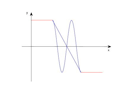
Figure 1.1: The function $f(x)$ and two different choices for $\left(f_{|_{R\setminus\mathcal{I}_{\Delta_{\varepsilon}}}}\right)_{e}$

We leave the reader to write the analytic expression of the functions and we stress the fact that $\left(f_{|_{R\setminus\mathcal{I}_{\Delta_{\varepsilon}}}}\right)_{e}$ is not uniquely identified by $\Delta_{\varepsilon}$.

We observe that

$$\lim_{\varepsilon\to 0^{+}}\underbrace{\int_{h}^{k}\left(f_{|_{R\setminus\mathcal{I}_{\Delta_{\varepsilon}}}}\right)_{e}(x)\;\mbox{\rm d}x}_{\tiny\begin{tabular}[]{l}Riemann integral\end{tabular}}=\underbrace{\int_{h}^{k}f(x)\;\mbox{\rm d}x}_{\tiny\begin{tabular}[]{l}Riemann integral\end{tabular}}$$

in spite of the fact that the convergence is not uniform.

This arguments is easily extended to functions with finitely many jumps, in particular to piecewise constant functions. We recall that the approximation from below and from above of a function with piecewise constant functions is the key step in the definition of the Riemann integral.   

Example 38 can be much strengthened:

Lemma 39

An a.e. continuous function which is a.e. defined on an interval $R$ is quasicontinuous.

Proof. We extend $f$ to ${\rm cl}\,R$ in an arbitrary fashion. The extension is still denoted $f$. By definition, for every $n$ there exists a multiinterval $\Delta$ such that $L(\Delta)<1/n$ and $f$ is continuous at the points of $R\setminus\mathcal{I}_{\Delta}$. So, $f_{|_{R\setminus\mathcal{I}_{\Delta}}}$ is continuous too. It follows that $f$ is quasicontinuous.   

The implication in Lemma 39 cannot be inverted:

Example 40

We noted that the Dirichlet function on $[0,1]$ is discontinuous at every point. Hence it is not a.e. continuous but it is quasicontinuous. In fact, we proved in the Example 12 that the set of the rational points of $[0,1]$ is a null set. So, for every $n$ there exists a multiinterval $\Delta_{n}$ such that $L(\Delta_{n})<1/n$ and $Q\subseteq\mathcal{I}_{\Delta_{n}}$.

The elements of the set $K_{n}=[0,1]\setminus\mathcal{I}_{\Delta_{n}}$ are irrational points and so

$$d_{|_{K_{n}}}(x)=0\quad\forall x\in K_{n}\,:$$

the function $d_{|_{K_{n}}}$ is constant, hence continuous. So, the Dirichlet function is quasicontinuous in spite of the fact that it is not a.e. continuous.

We note that the Tietze extension of $d_{|_{K_{n}}}$ is unique and it is identically zero:

$$(d_{|_{K_{n}}})_{e}=0$$

and this is a special instance of Lemma 31.   

The following simple observations have to be compared with Theorem 35.

Theorem 41

Let $R$ be an interval. The following properties hold:

1. let $f$ be quasicontinuous on $R$ and let $R_{1}\subseteq R$ ($R_{1}$ is an interval). Then $f_{|_{R_{1}}}$ is quasicontinuous on $R_{1}$.

2. let $\hat{h}\in(h,k)$. If $f$ is a.e. defined on $(h,k)$ and if it is quasicontinuous both on $(h,\hat{h})$ and on $(\hat{h},k)$ then it is quasicontinuous on $(h,k)$.

3. the sum and the product of two (bounded) quasicontinuous functions on an interval $R$ is a (bounded) quasicontinuous function on $R$.

   The quotient of quasicontinuous functions is quasicontinuous if the denominator is a.e. non zero.

4. let $f$ be quasicontinuouson the interval $R$ and let $g$ be a continuous function on a domain which contains the image of $f$. The composition $x\mapsto g(f(x))$ is quasicontinuous.

5. let $f_{n}$ be quasicontinuous functions. For every $k$, the functions

   $$\phi_{k}(x)=\max\{f_{1}(x)\,,\ f_{2}(x)\,,\ \dots\,,\ f_{k}(x)\}$$

   $$\psi_{k}(x)=\min\{f_{1}(x)\,,\ f_{2}(x)\,,\ \dots\,,\ f_{k}(x)\}$$

   are quasicontinuous.

These statements are either already noted or easily proved. In particular we examine the statement 5. It is sufficient to examine the maximum of two functions $f(x)$ and $g(x)$.

We use Theorem 25: if both $f(x)$ and $g(x)$ are continuous at $x_{0}$ then $x\mapsto\max\{f(x)\,,\ g(x)\}$ is continuous at $x_{0}$ too.

Let the two functions $f$ and $g$ be quasicontinuous on $R$. For every $\varepsilon>0$ there exists $\Delta_{\varepsilon}$ such that both $f_{R\setminus\Delta_{\varepsilon}}$ and $g_{R\setminus\Delta_{\varepsilon}}$ are continuous. The restriction to $R\setminus\Delta_{\varepsilon}$ of $\max\{f(x)\,,\ g(x)\}$ is equal to

$$\max\left\{f_{R\setminus\Delta_{\varepsilon}}\,,\ g_{R\setminus\Delta_{\varepsilon}}\right\}\,,$$

the maximum of two continuous functions. Hence, it is a continuous function.

Let now $\mathbbm{1}_{A}$ be the characteristic function of a set $A$:

$$\mathbbm{1}_{A}(x)=\left\{\begin{array}[]{lll}1&{\rm if}&x\in A\\ 0&{\rm if}&x\notin A\,.\end{array}\right.$$

The properties in the statements 1 and 2 of Theorem 41 can be recasted as follows:

Corollary 42

Let $f$ be a.e. defined on $[h,k]$ and let $\tilde{h}\in(h,k)$. The function $f$ is quasicontinuous if and only if both $\mathbbm{1}_{[h,\tilde{h}]}f$ and $\mathbbm{1}_{[\tilde{h},k]}f$ are quasicontinuous.

Now we recall the notations in (1.9) and observe that

$$f=\underbrace{f_{+,0}}_{=\max\{f,0\}}+\underbrace{f_{-,0}}_{=\min\{f,0\}}\,.$$

The previous result can be applied separately to $f_{+,0}$ and to $f_{-,0}$. We apply Theorems 25 and 41 to $f_{+,0}$ and to $f_{-,0}$ (when $A=R\setminus\mathcal{I}_{{\Delta_{\varepsilon}}}$). We find:

Theorem 43

Let the function $f$ be a.e. defined on $R$. Then we have:

1. the function $f$ is quasicontinuous if and only if both $f_{+,0}$ and $f_{-,0}$ are quasicontinuous.

2. if the function $f$ is quasicontinuous on an interval $R$ then $|f|$ is quasicontinuous on $R$ too.

Statement 2 follows from

$$|f(x)|=f_{+,0}(x)-f_{-,0}(x)\,.$$

Theorem 43 shows that it is not restrictive, when studying the properties of quasicontinuous functions, to assume that the functions do not change sign. This observation will be useful in the study of integration theory.

Remark 44

Observe that we did not assert that the composition of quasicontinuous function is quasicontinuous. In fact, in general it is not. See Remark 200 in Appendix 6.6.   

1.3.2 The Lebesgue Integral under Boundedness Assumptions

We define the Lebesgue integral of a bounded quasicontinuous function a.e. defined on a bounded interval.

We note a property of the Riemann integral:

Lemma 45

Let $f$ be Riemann integrable (hence bounded) on $[h,k]$ and let $|f(x)|\leq M$ for all $x\in[h,k]$. Let there exists a multiinterval $\Delta$ such that $f(x)=0$ if $x\in[h,k]\setminus\mathcal{I}_{\Delta}$. Then the following inequality holds for the Riemann integral:

$$\left|{\int_{h}^{k}f(x)\;\mbox{\rm d}x}\right|\leq ML(\Delta)\,.$$

Proof. The Riemann integral is

$$\int_{h}^{k}f(x)\;\mbox{\rm d}x=\lim_{N\to+\infty}\sum_{i=0}^{N-1}f(x_{i,N})(h_{i+1,N}-h_{i,N})$$ (1.20)

where $h_{i,N}=h+\dfrac{i}{N}(k-h)$ and $x_{N,i}\in[h_{i,N},h_{i+1,N})$ can be arbitrarily chosen (see Corollary 69 in Appendix 1.5). As the value of the integral does not depend on the choice of the points $x_{i,N}$ we decide to choose $x_{i,N}\notin\mathcal{I}_{\Delta}$ provided that this is possible, i.e. when $[h_{i,N},h_{i+1,N})$ is not contained in $\mathcal{I}_{\Delta}$.

This way, the nonzero elements of the right sum in (1.20) are those which corresponds to intervals $[h_{i,N},h_{i+1,N})$ which are contained in $\mathcal{I}_{\Delta}$. The sum of the lengths of these intervals is less then $L(\Delta)$ so that

$$\left|\sum_{i=0}^{N-1}f(x_{i,N})(h_{i+1,N}-h_{i,N})\right|\leq ML(\Delta)\,.$$

This inequality is preserved in the limit.   

We fix a bounded interval $R=[h,k]$ and a bounded quasicontinuous function $f$ a.e. defined on it:

$$|f(x)|<M\,.$$

Then we fix a sequence $(\Delta_{n},f_{n})$ of associated multiintervals and continuous functions of order $1/n$. The functions $f_{n}$ are continuous, hence Riemann integrable, on $R$.

Note that by the definition of the associated functions and from the inequality (1.19) we have

$$|f_{n}(x)|<M\qquad\forall x\in[h,k]\quad\forall n\,.$$ (1.21)

We prove:

Theorem 46

The sequence of the Riemann integrals

$$\int_{h}^{k}f_{n}(x)\;\mbox{\rm d}x$$

is convergent and the limit does not depend on the particular associated sequence $(\Delta_{n},f_{n})$ of order $1/n$ in the sense that if $(\hat{\Delta}_{n},\hat{f}_{n})$ is a different associated sequence of order $1/n$ then

$$\lim_{n\to+\infty}\int_{h}^{k}f_{n}(x)\;\mbox{\rm d}x=\lim_{n\to+\infty}\int_{h}^{k}\hat{f}_{n}(x)\;\mbox{\rm d}x\,.$$

Proof. The continuous function $f_{n}-f_{m}$ is different from zero solely on $\mathcal{I}_{\Delta_{n}}\cup\mathcal{I}_{\Delta_{m}}$. So, from Lemma 45, we have

$$\left|\int_{h}^{k}f_{n}(x)\;\mbox{\rm d}x-\int_{h}^{k}f_{m}(x)\;\mbox{\rm d}x\right|=\int_{h}^{k}|f_{n}(x)-f_{m}(x)|\;\mbox{\rm d}x\leq 2M\left(\frac{1}{n}+\frac{1}{m}\right)\,.$$

It follows that the sequence

$$\left\{\int_{h}^{k}f_{n}(x)\;\mbox{\rm d}x\right\}$$

is a Cauchy sequence, hence it is convergent.

In a similar way we see that the limit does not depend of the special associated sequence.

First we note that the inequalities (1.21) holds both for $f_{n}$ and for $\hat{f}_{n}$: if $|f(x)|<M$ then we have $|f_{n}(x)|<M$ and $|\hat{f}_{n}(x)|<M$ for every $n$. Then we observe

$$|f_{n}(x)-\hat{f}_{n}(x)|=0\quad\forall x\in[h,k]\setminus\left\{\mathcal{I}_{\Delta_{n}}\cup\mathcal{I}_{\hat{\Delta}_{n}}\right\}\,.$$

Hence

$$\left|\int_{h}^{k}f_{n}(x)\;\mbox{\rm d}x-\int_{h}^{k}\hat{f}_{n}(x)\;\mbox{\rm d}x\right|<\dfrac{4M}{n}$$

so that

$$\lim_{n\to+\infty}\left|\int_{h}^{k}f_{n}(x)\;\mbox{\rm d}x-\int_{h}^{k}\hat{f}_{n}(x)\;\mbox{\rm d}x\right|=0\,.\mbox{~{}~{}~{}~{}\rule{2.84526pt}{5.69054pt}\par\vskip 6.0pt plus 2.0pt minus 2.0pt}$$

It is clear that the special sequence $1/n$ has no role and the same argument can be repeated for sequences $(\Delta_{n},f_{n})$ of order $\varepsilon_{n}$ and $(\hat{\Delta}_{n},\hat{f}_{n})$ of order $\hat{\varepsilon}_{n}$ with $\varepsilon_{n}\to 0$ and $\hat{\varepsilon}_{n}\to 0$. I.e. we have

Theorem 47

Let $\{\varepsilon_{n}\}$ and $\{\hat{\varepsilon}_{n}\}$ be two sequences of positive numbers both convergent to zero. Let $f_{n}$, $\hat{f}_{n}$ be associated continuous functions (to $f$) of order respectively to $\varepsilon_{n}$ and to $\hat{\varepsilon}_{n}$. Then we have

$$\lim_{n\to+\infty}\int_{h}^{k}f_{n}(x)\;\mbox{\rm d}x=\lim_{n\to+\infty}\int_{h}^{k}\hat{f}_{n}(x)\;\mbox{\rm d}x\,.$$

These observations justify the following definition: let $f$ be a bounded quasicontinuous function a.e. defined on the bounded interval $R=[h,k]$. We fix any sequence $\{\Delta_{n},f_{n}\}$ of associated multiintervals and continuous functions of order $1/n$. The Lebesgue integral of $f$ on $R$ is defined as follows

$$\underbrace{\int_{h}^{k}f(x)\;\mbox{\rm d}x}_{\tiny\begin{tabular}[]{l}Lebesgue\\ integral\end{tabular}}=\lim_{n\to+\infty}\underbrace{\int_{h}^{k}f_{n}(x)\;\mbox{\rm d}x}_{\tiny\begin{tabular}[]{l}Riemann\\ integral\end{tabular}}\,.$$ (1.22)

A consequence of the fact that $f$ is only a.e. defined on $R$ is that the integral does not change if the interval $R$ is open or half open.

Example 48

Let us see two examples:

1. Let $f$ be a.e. defined on $[h,k]$, and let

   $$f(x)=f_{1}\quad h\leq x<\tilde{h}\,,\qquad f(x)=f_{2}\quad\tilde{h}<x<k\,.$$

   Tietze extensions of this functions have been considered in Example 38. From the arguments in Example 38 we see that the Lebesgue integral of $f$ is

   $$\int_{h}^{k}f(x)\;\mbox{\rm d}x=f_{1}(\tilde{h}-h)+f_{2}(k-\tilde{h})\,.$$

   It is known that the sum on the right is also the Riemann integral of the function.

   This observation can be extended to any piecewise continuous function. Let $h_{i}$, $0\leq i\leq N$ be points such that

   $$h=h_{0}\,,\quad h_{i}\leq h_{i+1}\,,\quad h_{N}=k$$

   and let $\chi(x)=\chi_{i}$ if $x\in[h_{i},h_{i+1})$. Then, its Lebesgue integral is

   $$\int_{h}^{k}\chi(x)\;\mbox{\rm d}x=\sum_{i=0}^{N}\chi_{i}(h_{i+1}-h_{i})$$

   and this number is also the Riemann integral of $\chi$.

2. Example 40 shows that

   $$\underbrace{\int_{h}^{k}d(x)\;\mbox{\rm d}x}_{\tiny\begin{tabular}[]{l}Lebesgue integral\end{tabular}}=0\quad\mbox{($d$ is the Diriclet function)}$$

   as required in Remark 6.   

The definition of the oriented Riemann integral suggests to define also of the oriented Lebesgue integral:

$$\underbrace{\int_{h}^{k}f(x)\;\mbox{\rm d}x=-\int_{k}^{h}f(x)\;\mbox{\rm d}x}_{\rm Lebesgue\ integrals}\quad\mbox{since}\quad\underbrace{\int_{h}^{k}f_{n}(x)\;\mbox{\rm d}x=-\int_{k}^{h}f_{n}(x)\;\mbox{\rm d}x}_{\rm Riemann\ integrals}\,.$$

When the interval of endpoints $h$ and $k$ (with $h\leq k$) is denoted $R$ then we use, both for the Riemann and the Lebesgue integrals,

$$\int_{R}f(x)\;\mbox{\rm d}x\quad\mbox{to denote}\quad\int_{h}^{k}f(x)\;\mbox{\rm d}x\qquad\mbox{(we repeat: $h\leq k$)}\,.$$

From now on, the integral sign will always denote the Lebesgue integral, unless explicitly stated that it is a Riemann integral. The fact that $\int$denotes a Lebesgue integral is explicitly indicated when convenient for clarity.

Now we state the following obvious result (recall Example 48 for the second statement and Lemma 31 for the third):

Theorem 49

We have:

1. any $f\in C([h,k])$ is Lebesgue integrable and its Lebesgue integral coincide with its Riemann integral. In particular, if $f(x)\equiv c$ on $[h,k]$ then its Lebesgue integral is $c(k-h)$.

2. any piecewise continuous function is Lebesgue integrable and its Lebesgue integral coincides with its Riemann integral.

3. two functions which are a.e. equal on $R$ have the same Lebesgue integral. In particular

   $$f=0\ {\rm a.e.}\ x\in[h,k]\ \ \implies\ \ \int_{h}^{k}f(x)\;\mbox{\rm d}x=0\,.$$

The following result is a simple consequence of the corresponding result which holds for the Riemann integral of continuous functions:

Theorem 50

Let $f$ and $g$ be a.e. defined on $[h,k]$, bounded and quasicontinuous. Then:

1. linearity of the integral: if $\alpha$ e $\beta$ are real numer then

   $$\int_{h}^{k}\left(\alpha f(x)+\beta g(x)\right)\;\mbox{\rm d}x=\alpha\int_{h}^{k}f(x)\;\mbox{\rm d}x+\beta\int_{h}^{k}g(x)\;\mbox{\rm d}x\,.$$

2. additivity of the integral: if  $\hat{h}\in(h,k)$ then

   $$\int_{h}^{k}f(x)\;\mbox{\rm d}x=\int_{h}^{\hat{h}}f(x)\;\mbox{\rm d}x+\int_{\hat{h}}^{k}f(x)\;\mbox{\rm d}x\,.$$

3. monotonicity of the integral: if $f(x)\leq g(x)$ then

   $$\int_{h}^{k}f(x)\;\mbox{\rm d}x\leq\int_{h}^{k}g(x)\;\mbox{\rm d}x\,.$$

4. inequality for the absolute value: we have

   $$\left|\int_{h}^{k}f(x)\;\mbox{\rm d}x\right|\leq\int_{h}^{k}|f(x)|\;\mbox{\rm d}x\,.$$

5. integrability of the product and of the quotient: the product $f(x)g(x)$ is integrable; the quotient $f(x)/g(x)$ is integrable provided that $|g(x)|>\alpha>0$.

Remark 51

The monotonicity property requires the following comment. By definition, the value of the Lebesgue integral is the limit of the sequence on the right side of (1.22) and it does not depend on the sequence that it is used. So, monotonicity easily follows if we use the associated sequences to $f$ and $g$ used in the proof of Theorem 30 since in this case $f(x)\geq g(x)$ implies $f_{n}(x)\geq g_{n}(x)$ (see the statement 1 of Theorem 33).   

We note the following equality which holds for the Riemann integral:

$$\int_{h+\alpha}^{k+\alpha}f(x-\alpha)\;\mbox{\rm d}x=\int_{h}^{k}f(x)\;\mbox{\rm d}x\,.$$ (1.23)

Passing to the limit of sequences of associated functions we see that the property (1.23) holds also for the Lebesgue integral.

Equality (1.23) is the translation invariance of the (Riemann or Lebesgue) integral.

As stated in Theorem 49, continuous functions and piecewise constant functions (on a bounded interval) are both Riemann and Lebesgue integrable and the two integrals have the same value. In fact, the Lebesgue integral extends the Riemann integral since:

Theorem 52

Every Riemann integrable function is bounded quasicontinuous, hence Lebesgue integrable, and the values of its Riemann and Lebesgue integrals coincide. The proof is in Appendix 1.5.2 where we prove also:

Theorem 53

A bounded function defined on a bounded interval is Riemann integrable if and only if the set of its points of discontinuity is a null set.

1.3.3 The Integral of Unbounded Functions on Unbounded Domains

First we investigate the definition of the integral of a function $f$ which is a.e. defined on $\mathbb{R}$ and which can be unbounded. Then we consider the integral of $f$ on a set $A$ provided that $A$ has a suitable property.

So, we proceed in two steps:

Step 1:

We put

$$f_{+}(x)=f_{+,0}(x)=\max\{f(x),0\}\,,\qquad f_{-}(x)=f_{-,0}(x)=\min\{f(x),0\}$$

so that $f_{+}(x)\geq 0$ and $f_{-}(x)\leq 0$ for every $x$. Then, when $N\geq 0$, $K\geq 0$ and $R>0$, we put

$$f_{+;\,(R,N)}(x)=\left\{\begin{array}[]{lll}\min\{f_{+}(x)\,,\ N\}&{\rm if}&|x|<R\\ 0&{\rm if}&|x|\geq R\,.\end{array}\right.$$

$$f_{-;\,(R,-K)}(x)=\left\{\begin{array}[]{lll}\max\{f_{-}(x)\,,\ -K\}&{\rm if}&|x|<R\\ 0&{\rm if}&|x|\geq R\,.\end{array}\right.$$

Step 1A:

Since $f$ is quasicontinuous, the function $f_{+;\,(R,N)}$ is bounded quasicontinuous for every $R$ and every $N$. We define

$$\underbrace{\int_{\mathbb{R}}f_{+}(x)\;\mbox{\rm d}x}_{\tiny\begin{tabular}[]{l}Lebesgue\\ integral\end{tabular}}=\lim_{\stackrel{{\scriptstyle R\to+\infty}}{{N\to+\infty}}}\underbrace{\int_{-R}^{R}f_{+;\,(R,N)}(x)\;\mbox{\rm d}x}_{\tiny\begin{tabular}[]{l}Lebesgue\\ integral\end{tabular}}\,.$$ (1.26)

The limit has to be computed with $(R,N)\in\mathbb{N}\times\mathbb{N}$ (i.e. one independent from the other). It exists since $f_{+;\,(R,N)}\geq 0$ and it can be $+\infty$.

Step 1B:

Since $f$ is quasicontinuous, the function $f_{-;\,(R,-K)}$ is bounded quasicontinuous for every $R$ and every $K$. We define

$$\underbrace{\int_{\mathbb{R}}f_{-}(x)\;\mbox{\rm d}x}_{\tiny\begin{tabular}[]{l}Lebesgue\\ integral\end{tabular}}=\lim_{\stackrel{{\scriptstyle R\to+\infty}}{{K\to+\infty}}}\underbrace{\int_{-R}^{R}f_{-;\,(R,-K)}(x)\;\mbox{\rm d}x}_{\tiny\begin{tabular}[]{l}Lebesgue\\ integral\end{tabular}}\,.$$ (1.27)

The limit has to be computed with $(R,K)\in\mathbb{N}\times\mathbb{N}$ (i.e. one independent from the other) and it can be $-\infty$.

Step 1C:

the quasicontinuous function $f$ is integrable on $\mathbb{R}$ when at least one of the functions $f_{+}$ or $f_{-}$ has finite integral.

In this case we define

$$\underbrace{\int_{\mathbb{R}}f(x)\;\mbox{\rm d}x}_{\tiny\begin{tabular}[]{l}Lebesgue\\ integral\end{tabular}}=\underbrace{\int_{\mathbb{R}}f_{+}(x)\;\mbox{\rm d}x}_{\tiny\begin{tabular}[]{l}Lebesgue\\ integral\end{tabular}}+\underbrace{\int_{\mathbb{R}}f_{-}(x)\;\mbox{\rm d}x}_{\tiny\begin{tabular}[]{l}Lebesgue\\ integral\end{tabular}}\,.$$ (1.28)

The integral can be a number (when both the integrals of $f_{+}$ and of $f_{-}$ are numbers) or it can be $+\infty$ or it can be $-\infty$.

If the integral is a number, then we say that $f$ is summable.

Step 2:

let $A\subseteq\mathbb{R}$ satisfy the following assumption:

Assumption 54

The characteristic function of the set $A$ is quasicontinuous.   

When $f$ is quasicontinuous on $\mathbb{R}$ and the set $A$ satisfies the Assumption 54 then the product $f\mathbbm{1}_{A}$ is quasicontinuous. With an abuse of notation, even if $f$ is solely a.e. defined on $A$ we put

$$f(x)\mathbbm{1}_{A}(x)=\left\{\begin{array}[]{lll}f(x)&{\rm if}&x\in A\\ 0&{\rm if}&x\notin A\end{array}\right.\qquad\mbox{(abuse of notations)}$$ (1.29)

and:

1. if $f\mathbbm{1}_{A}$ (defined as in (1.29)) is quasicontinuous on $\mathbb{R}$ we say that $f$ is a quasicontinuous function on $A$;

2. if $f\mathbbm{1}_{A}$ is integrable on $\mathbb{R}$ then we say that $f$ is integrable on the set A; if it is summable then we say that $f$ is summable on the set A;

3. if $f$ is integrable or summable on $A$ then we introduce the notation

   $$\int_{A}f(x)\;\mbox{\rm d}x=\int_{\mathbb{R}}f(x)\mathbbm{1}_{A}(x)\;\mbox{\rm d}x\,.$$

Remark 55

We note:

1. sets which do not satisfy Assumption 54 exist. An example is in the Appendix 6.5.

2. any open set satisfies Assumption 54. A faulty proof is as follows: let ${\mathcal{O}}=\cup_{n\geq 1}(a_{n},b_{n})$ and let the intervals be pairwise disjoint. The function $\mathbbm{1}_{\mathcal{O}}$ is discontinuous at $a_{n}$ and at $b_{n}$. The set of the points $a_{n}$ and $b_{n}$ is numerable so that $\mathbbm{1}_{\mathcal{O}}$ is discontinuous on a numerable set. Hence, $\mathbbm{1}_{\mathcal{O}}$ is quasicontinuous. We invite the reader to discuss the error in this argument. The error is discussed in Remark 196 while a correct proof is in Theorem 88.   

The following properties of the integral clearly holds:

Theorem 56

Let $A$ be a set which satisfies the Assumption 54 and let $f$ and $g$ be summable on $A$. Then:

1. linearity of the integral: if $\alpha$ e $\beta$ are real numbers the function $\alpha f+\beta g$ is summable and

   $$\int_{A}\left(\alpha f(x)+\beta g(x)\right)\;\mbox{\rm d}x=\alpha\int_{A}f(x)\;\mbox{\rm d}x+\beta\int_{h}^{k}g(x)\;\mbox{\rm d}x\,.$$

2. if $g$ is bounded then the product $fg$ is summable; if $1/g$ is bounded then the quotient $f/g$ is summable.

3. monotonicity of the integral: if $f(x)\leq g(x)$ then

   $$\int_{A}f(x)\;\mbox{\rm d}x\leq\int_{A}g(x)\;\mbox{\rm d}x\,.$$

4. two functions which are a.e. equal on $R$ have the same Lebesgue integral. In particular the integral of a function which is a.e. zero is equal to zero.

The previous properties correspond to properties which hold also for the improper integral. Instead, the absolute value has a new and an important property.

Theorem 57

We have:

1. If $f$ is integrable then $|f|$ is integrable and

   $$\int_{A}|f(x)|\;\mbox{\rm d}x=\int_{A}f_{+}(x)\;\mbox{\rm d}x-\int_{A}f_{-}(x)\;\mbox{\rm d}x\,.$$

   So, the usual inequality of the absolute value holds:

   $$\left|\int_{A}f(x)\;\mbox{\rm d}x\right|\leq\int_{A}|f(x)|\;\mbox{\rm d}x\,.$$

2. Let the function $f$ be quasicontinuous. It is summable if and only if $|f|$ is summable.

We stress the assumption that $f$ is quasicontinuous in the statement 2. This assumption cannot be removed since we shall see in the Remark 199 of the Appendix 6.5 the existence of functions which are not quasicontinuous but whose absolute value is constant.

The last statement of Theorem 57 is crucial in functional analysis, since it permits to define integral norms and the spaces $L^{p}$.

Finally we state the translation invariance and the additivity of the integral.

Theorem 58

The following properties hold:

1. translation invariance: let $A$ be a set which satisfies the Assumption 54 and let $f$ be defined on $A$ and quasicontinuous. Let $\alpha\in\mathbb{R}$ and

   $$A+\alpha=\{x+\alpha\,,\ x\in A\}\,.$$

   We have:

   1. the set $A+\alpha$ satisfies the Assumption 54 and the function $x\mapsto f(x-\alpha)$ (defined on $A+\alpha$) is quasicontinuous.

   2. if $f$ is integrable on $A$ then we have:

      $$\int_{A+\alpha}f(x-\alpha)\;\mbox{\rm d}x=\int_{A}f(x)\;\mbox{\rm d}x\,.$$

2. additivity of the integral: let $A_{1}$ and $A_{2}$ be two disjoint sets which satisfy Assumption 54 and let $f$ be defined on $A_{1}\cup A_{2}$. We assume that $f_{|_{A_{1}}}$ and $f_{|_{A_{2}}}$ are summable (hence also quasicontinuous). We have:

   1. the set $A_{1}\cup A_{2}$ satisfy Assumption 54 and $f$ is summable on $A_{1}\cup A_{2}$.

   2. we have

      $$\int_{A_{1}\cup A_{2}}f(x)\;\mbox{\rm d}x=\int_{A_{1}}f(x)\;\mbox{\rm d}x+\int_{A_{2}}f(x)\;\mbox{\rm d}x\quad\mbox{(recall: $A_{1}\cap A_{2}=\emptyset$)}\,.$$

3. if $A_{1}\cap A_{2}\neq\emptyset$ then:

   1. the sets $A_{1}\cap A_{2}$, $A_{1}\setminus A_{2}$ and $A_{2}\setminus A_{1}$ (if nonempty) satisfy Assumption 54;

   2. if $f$ is defined on $A_{1}\cup A_{2}$ and $f_{|_{A_{1}}}$ and $f_{|_{A_{2}}}$ are summable then $f$ is summable on $A_{1}\cup A_{2}$ and

      $$\int_{A_{1}\cup A_{2}}f(x)\;\mbox{\rm d}x\leq\int_{A_{1}}f(x)\;\mbox{\rm d}x+\int_{A_{2}}f(x)\;\mbox{\rm d}x\,.$$

Note that the statement 3 is consequence of the additivity of the integral since

$$A_{1}\cup A_{2}=(A_{1}\setminus A_{2})\cup(A_{1}\cap A_{2})\cup(A_{2}\setminus A_{1})\quad\mbox{(disjoint union)}$$

and

$$\mathbbm{1}_{A_{1}\cap A_{2}}(x)=\mathbbm{1}_{A_{1}}(x)\mathbbm{1}_{A_{2}}(x)\,,\qquad\mathbbm{1}_{A_{1}\setminus A_{2}}(x)=\max\{\mathbbm{1}_{A_{1}}(x)-\mathbbm{1}_{A_{2}}(x),0\}\,.$$

We conclude with two simple observations where we use the notation

$$f_{-,N}(x)=\min\{f(x),N\}\,.$$

The theorem on the limits of monotone functions shows the following criterion of summability:

Theorem 59

The quasicontinuous function $f$ is summable if and only if the function

$$(N,R)\mapsto\int_{-R}^{R}|f|_{-,N}(x)\;\mbox{\rm d}x$$

(defined for $N>0$ and $R>0$) is bounded.

The second observation is a consequence of the linearity and additivity of the integral:

Theorem 60

Let $f\geq 0$ be summable. For every $\varepsilon>0$ there exists $N_{\varepsilon}$ and $R_{\varepsilon}$ such that:

• if $N>N_{\varepsilon}$ we have $\int_{A}\left[f(x)-f_{-,N}(x)\right]\;\mbox{\rm d}x<\varepsilon$.

• if $R>R_{\varepsilon}$ we have $\int_{|R|>R_{\varepsilon}}f(x)\;\mbox{\rm d}x<\varepsilon$.

Lebesgue Integral and Improper Integral

Theorem 52 (yet to be proved) shows that Riemann integral is extended and superseded by the Lebesgue integral. Instead, the Lebesgue integral for unbounded functions or on unbounded intervals does not supersede the improper integral since there exist even continuous functions which are important for the applications and which admit improper integral but which are not Lebesgue summable. Important examples are the improper integral of the $\operatorname{sinc}$ function and the Fresnel integrals:

$$\underbrace{\int_{-\infty}^{+\infty}\operatorname{sinc}\pi x\;\mbox{\rm d}x}_{\tiny\begin{tabular}[]{l}improper\\ integral\end{tabular}}=\underbrace{\int_{-\infty}^{+\infty}\frac{\sin\pi x}{\pi x}\;\mbox{\rm d}x}_{\tiny\begin{tabular}[]{l}improper\\ integral\end{tabular}}=1\,,$$

$$\underbrace{\int_{-\infty}^{+\infty}\sin^{2}x}_{\tiny\begin{tabular}[]{l}improper\\ integral\end{tabular}}\;\mbox{\rm d}x=\underbrace{\int_{-\infty}^{+\infty}\cos x^{2}\;\mbox{\rm d}x}_{\tiny\begin{tabular}[]{l}improper\\ integral\end{tabular}}=\sqrt{\dfrac{\pi}{2}}\,.$$

1.4 Limits and the Integral

Both the definition of the Riemann and the Lebesgue integrals have a common idea: first we single out a class of “simple” functions whose integral can be defined in an obvious way. Then we single out classes of functions which can be “approximated” with simple functions. Let $f$ be a function in this class and $\{s_{n}\}$ be a sequence of “approximating” functions. We prove that the integrals of the functions $s_{n}$ converge to a number which is chosen as the (Riemann or Lebesgue) theorem of $f$.

In the case of the Riemann integral, the simple functions are piecewise constant and the Riemann integrable functions $f$ have to be uniformly approximated by piecewise constant function. So, it is natural to expect that limits and integrals can be exchanged when “convergence” is uniform convergence.

In the case of the Lebesgue integrals, the “simple” functions are continuous functions but the “approximation” is more general then pointwise convergence on an interval: it is “approximation” in the weaker sense of the existence of sequences of associated functions. So, it is natural to expect that limits and integrals can be exchanged under more general conditions. In fact we have the results which we state here and we prove in Chap. 2.

The first result shows that the request 4 in the Table 1.1 is satisfied by the Lebesgue interval. The proof is in Chap. 2 but, for the convenience of the readers who do not plan to study Chap. 2, at the end of this section we sketch the proof under restrictive assumptions.

Theorem 61

Let $\{f_{n}\}$ be a bounded sequence of quasicontinuous function defined on a bounded interval $[h,k]$.

Let $\{f_{n}(x)\}$ converges to $f(x)$ a.e. on $[h,k]$. Then the function $f$ is bounded quasicontinuous and we have

$$\lim_{n\to+\infty}\left[\int_{h}^{k}f_{n}(x)\;\mbox{\rm d}x\right]=\int_{h}^{k}\left[\lim_{n\to+\infty}f_{n}(x)\right]\;\mbox{\rm d}x=\int_{h}^{k}f(x)\;\mbox{\rm d}x\,.$$

The heavy boundedness assumptions in this theorem can be much relaxed and in fact we have:

Theorem 62 (Beppo Levi or monotone convergence)

Let $\{f_{n}\}$ be a sequence of integrable functions defined a.e. on $\mathbb{R}$ and let us assume that the following properties hold a.e. on $\mathbb{R}$:

$${\bf 1)}\quad 0\leq f_{n}(x)\leq f_{n+1}(x)\,, {\bf 2)}\quad\lim_{n\to+\infty}f_{n}(x)=f(x)\qquad a.e.\ x\in\mathbb{R}\,.$$

Then, $f$ is integrable and

$$\lim_{n\to+\infty}\int_{-\infty}^{+\infty}f_{n}(x)\;\mbox{\rm d}x=\int_{-\infty}^{+\infty}f(x)\;\mbox{\rm d}x\,.$$

Note that in this theorem the functions $f_{n}$ need not be summable. The assumption is that they are integrable. And the conclusion is that $f$ is integrable, possibly not summable. The function $f$ may not be summable even if each one of the functions $f_{n}$ is.

Concerning summability we have:

Theorem 63 (Lebesgue or dominated convergence)

Let $\{f_{n}\}$ be a sequence of summable functions a.e. defined on $\mathbb{R}$ and let $f_{n}\to f$ a.e. on $\mathbb{R}$. If there exists a summable nonnegative function $g$ such that

$$|f_{n}(x)|\leq g(x)\qquad a.e.\ x\in\mathbb{R}$$

then $f(x)$ is summable and

$$\lim\int_{-\infty}^{+\infty}f_{n}(x)\;\mbox{\rm d}x=\int_{-\infty}^{+\infty}f(x)\;\mbox{\rm d}x\,.$$

Sketch of the proof of Theorem 61

We assume that the assumptions of the theorem hold and furthermore that a seemingly restrictive assumption holds too. So we assume:

1. each function $f_{n}$ is a.e. defined on $[h,k]$ and it is quasicontinuous.

2. there exists $M$ such that $|f_{n}(x)|<M$ a.e. $x\in[h,k]$ and for every $n$.

3. the sequence converges a.e. $x\in[h,k]$, $f_{n}(x)\to f(x)$.

4. for every $\varepsilon>0$ there exists a multiinterval $\Delta_{\varepsilon}$ such that $L(\Delta_{\varepsilon})<\varepsilon$ and such that every $f_{n}$ is defined on $[h,k]\setminus\mathcal{I}_{\Delta_{\varepsilon}}$ and furthermore:

   1. the restriction $(f_{n})_{|_{[h,k]\setminus\mathcal{I}_{\Delta_{\varepsilon}}}}$ is continuous.

   2. the sequence $\{f_{n}\}$ is uniformly convergent on $[h,k]\setminus\mathcal{I}_{\Delta_{\varepsilon}}$.

Assumption 4 looks unduly restrictive but Egorov-Severini Theorem (Theorem 83 of Chap. 2) shows that it is a consequence of pointwise convergence.

The key points of the proof of Theorem 61 are the following ones.

The limit function $f$ is quasicontinuous.

We use the assumption 4: we fix $\varepsilon>0$ and a corresponding multiinterval $\Delta_{\varepsilon}$. In order to simplify the following notations, we put

$$H_{\varepsilon}=[h,k]\setminus\mathcal{I}_{\Delta_{\varepsilon}}\quad\mbox{(note that $H_{\varepsilon}$ is closed)}\,.$$

We associate to the restriction of $f_{n}$ to $H_{\varepsilon}$ the particular Tietze extension constructed in Theorem 30, via linear interpolation. This particular Tietze extension is denoted $f_{n,\varepsilon,e}$.

Now we use the following steps:

1. Assumption 4 and the statement 2 of Theorem 33 imply that the sequence $n\mapsto f_{n,\varepsilon,e}(x)$ is convergent for every $x\in[h,k]$. Let $\hat{f}$ be the limit function.

2. Assumption 4 implies that the sequence $\{(f_{n})_{|_{H_{\varepsilon}}}\}$ is uniformly convergent and it is a sequence of continuous functions. So, its limit $\hat{f}_{|_{H_{\varepsilon}}}$ is continuous.

3. from $(f_{n})_{|_{H_{\varepsilon}}}(x)=f_{n}(x)$ and $f_{n}(x)\to f(x)$ for every $x\in H_{\varepsilon}$, it follows that $\hat{f}(x)=f(x)$ if $x\in H_{\varepsilon}$.

   So, $f_{|_{H_{\varepsilon}}}$ is continuous and $\hat{f}$ is one of its Tietze extensions.

   This argument holds for every $\varepsilon>0$ and so $f$ is quasicontinuous.

We prove convergence of the integrals.

Once quasicontinuity of $f$ is known we can replace $f_{n}$ with $f_{n}-f$ and we can assume $f_{n}\to 0$.

We prove that if $f_{n}\to 0$ a.e. then the sequence of the integrals converges to zero.

Assumption 4 and Theorem 32 imply that $\{f_{n,\varepsilon,e}\}$ converges uniformly to $0$.

We note

$$\underbrace{\int_{h}^{k}f_{n}(x)\;\mbox{\rm d}x}_{\tiny\begin{tabular}[]{l}Lebesgue integral\end{tabular}}=\overbrace{\underbrace{\int_{h}^{k}f_{n,\varepsilon,e}(x)\;\mbox{\rm d}x}_{A}}^{\tiny\begin{tabular}[]{l}Riemann integral\end{tabular}}+\overbrace{\underbrace{\int_{h}^{k}\left[f_{n}(x)-f_{n,\varepsilon,e}(x)\right]\;\mbox{\rm d}x}_{B}}^{\tiny\begin{tabular}[]{l}Lebesgue integral\end{tabular}}\,.$$

The difference $\left[f_{n}(x)-f_{n,\varepsilon,e}(x)\right]$ is zero when $x\notin\mathcal{I}_{\Delta_{\varepsilon}}$. This fact implies

$$|B|\leq 2M\varepsilon\,.$$

The integrals $A$ are Riemann integrals and the integrands converge uniformly to zero. So, $|A|$ can be made as small as we wish by taking $n$ large.

This implies that for every $\sigma>0$ and every $\varepsilon>0$ there exists $N=N_{\sigma,\varepsilon}$ such that if $n>N_{\sigma,\varepsilon}$ we have

$$\left|\int_{h}^{k}f_{n}(x)\;\mbox{\rm d}x\right|\leq|A|+|B|<\sigma+\varepsilon\,,$$

as wanted.

1.5 Appendix: Riemann and Lebesgue Integrals

In this appendix we sketch the definition of the Riemann integral and we characterize Riemann integrability of a function in terms of its points of discontinuity. Then we prove that every Riemann integrable function is Lebesgue integrable and that the two integrals have the same value.

1.5.1 A Sketch of the Riemann Integral

Functions which are Riemann integrable must be bounded and defined on a bounded interval which we denote $[h,k]$ but the fact that the end points belong to the interval has no effect on integrability of the function or on the value of its Riemann integral.

We sketch the definition of the Riemann integral and the relation of the Riemann integral with the oscillation of the function.

The Oscillation of a Function

We define the oscillation of a function on a set and at a point.

Let $f$ be a real valued function defined on a subset $A\subseteq\mathbb{R}$. Let $U$ be a set which intersects $A$: $A\cap U\neq\emptyset$. The oscillation of $f$ on $U$ is

$$\Omega(f,U)=\left[\sup_{x\in A\cap U}f(x)-\inf_{x\in A\cap U}f(x)\right]\,.$$

We fix a point $x_{0}\in{\rm cl}\,A$ and we consider the intervals $B(x_{0},r)=(x_{0}-r,x_{0}+r)$ i.e. the neighborhood of $x_{0}$ of radius $r$. The function

$$r\mapsto\Omega(f,B(x_{0},r))$$

is increasing, hence we can define the oscillation of $f$ at $x_{0}$ as

$$\omega(f;x_{0})=\lim_{r\to 0^{+}}\Omega\left(f,B(x_{0},r)\right)\,.$$

The oscillation can be used to characterize continuity:

Theorem 64

Let $x_{0}\in A={\rm dom}\,f$. The function $f$ is continuous at $x_{0}$ if and only if $\omega(f;x_{0})=0$.

Proof. Let $f$ be continuous at $x_{0}$ and let $\varepsilon>0$. There exists $N$ such that for every $n>N$ the condition $|x-x_{0}|<1/n$ implies $|f(x)-f(x_{0})|<\varepsilon$. So,

$$|x-x_{0}|<\dfrac{1}{n}\,,\quad|y-x_{0}|<\dfrac{1}{n}\ \implies\ |f(x)-f(y)|<2\varepsilon$$

and so

$$n>N_{\varepsilon}\ \implies\ \Omega\left(f,B(x_{0},1/n)\right)<2\varepsilon\,.$$

Then we have $\omega(f;x_{0})=0$ since $\varepsilon>0$ is arbitrary.

Conversely, let $\omega(f;x_{0})=0$. Then, for every $\varepsilon>0$ there exists $\delta>0$ such that

$$0<r<\delta\ \implies\ \Omega\left(f,B(x_{0},r)\right)<\varepsilon\,.$$

$$\mbox{In particular if $x\in B(x_{0},r)$ then}\quad|f(x)-f(x_{0})|\leq\Omega(f,B(x_{0},r))<\varepsilon\,.\mbox{~{}~{}~{}~{}\rule{2.84526pt}{5.69054pt}\par\vskip 6.0pt plus 2.0pt minus 2.0pt}$$

We shall use the following result:

Theorem 65

Let $f$ be any function defined on $[h,k]$ and let $\alpha\geq 0$. The set

$$A_{\alpha}=A_{f,\alpha}=\{x\in[h,k]\,:\ \omega(f;x)\geq\alpha\}$$ (1.30)

is closed.

Proof. We prove that if $\hat{x}$ is an accumulation point of $A_{\alpha}$ then it belongs to $A_{\alpha}$ i.e. we prove that

$$\omega(f;\hat{x})\geq\alpha\,.$$

The neighborhood $B(\hat{x},1/n)$ contains a point $\tilde{x}\in A_{\alpha}$ and it contains also a neighborhood $U$ of $\tilde{x}$. So,

$$\Omega\left(f,B(\hat{x},1/n)\right)=\left[\sup_{x\in B(\hat{x},1/n)}f(x)-\inf_{x\in B(\hat{x},1/n)}f(x)\right]\\ \geq\left[\sup_{x\in U}f(x)-\inf_{x\in U}f(x)\right]\geq\omega(f;\tilde{x})\geq\alpha\,.$$

The inequality is preserved by the limit so that

$$\omega(f;\hat{x})=\lim_{n\to+\infty}\left[\sup_{x\in B(\hat{x},1/n)}f(x)-\inf_{x\in B(\hat{x},1/n)}f(x)\right]\geq\alpha\,.\mbox{~{}~{}~{}~{}\rule{2.84526pt}{5.69054pt}\par\vskip 6.0pt plus 2.0pt minus 2.0pt}$$

Riemann Integral: the Conditions of Integrability

Riemann integral of the bounded function $f$ defined on the bounded interval $[h,k]$ can be defined with several slightly different but equivalent methods. We sketch one.

In the contest of Riemann integral, a partition of $[h,k]$ is a finite set $\mathcal{P}=\{h_{i}\}_{0\leq i\leq N}$ such that

$$h_{0}=h\,,\quad h_{i}<h_{i+1}\,,\quad h_{N}=k\,.$$

We associate to the partition $\mathcal{P}$ the following numbers

$$\begin{array}[]{ll}\displaystyle\par l_{i}=h_{i+1}-h_{i}\,,&\delta(\mathcal{P})=\max\{l_{i}\}\\[5.69054pt] \displaystyle m_{i}=m_{i,\cal{P}}=\inf_{x\in[h_{i},h_{i+1})}f(x)\,,&M_{i}=M_{i,\mathcal{P}}=\sup_{x\in[h_{i},h_{i+1})}f(x)\,.\end{array}$$

Then we introduce the two piecewise constant functions $\chi_{+,\mathcal{P}}$ and $\chi_{-,\mathcal{P}}$

$$\mbox{if $x\in[h_{i},h_{i+1})$ then}\ \left\{\begin{array}[]{l}\chi_{+,\mathcal{P}}(x)=M_{i}\,,\\ \chi_{-,\mathcal{P}}(x)=m_{i}\,.\end{array}\right.$$

As seen in Example 48, their Lebesgue integrals are the numbers

$$\begin{array}[]{ll}\displaystyle I_{+}(f,\mathcal{P})&=\underbrace{\int_{h}^{k}\chi_{+,\mathcal{P}}(x)\;\mbox{\rm d}x}_{\tiny\begin{tabular}[]{l}Lebesgue\\ integral\end{tabular}}=\sum_{i=0}^{N-1}M_{i}(h_{i+1}-h_{i})\,,\\[8.53581pt] \displaystyle I_{-}(f,\mathcal{P})&=\underbrace{\int_{h}^{k}\chi_{-,\mathcal{P}}(x)\;\mbox{\rm d}x}_{\tiny\begin{tabular}[]{l}Lebesgue\\ integral\end{tabular}}=\sum_{i=0}^{N-1}m_{i}(h_{i+1}-h_{i})\,.\end{array}$$ (1.31)

It is clear that $I_{-}(f,\mathcal{P})\leq I_{+}(f,\mathcal{P})$ and in fact we have also

$$I_{-}(f,\mathcal{P})\leq I_{+}(f,\mathcal{Q})$$

even if $\mathcal{P}$ and $\mathcal{Q}$ are different partitions.

By definition, the function $f$ is Riemann integrable when

$$\sup\{I_{-}(f,\mathcal{P})\}=\inf\{I_{+}(f,\mathcal{P})\}$$

and this number is its Riemann integral:

$$\underbrace{\int_{h}^{k}f(x)\;\mbox{\rm d}x}_{\tiny\begin{tabular}[]{l}Riemann\\ integral\end{tabular}}=\sup\{I_{-}(f,\mathcal{P})\}=\inf\{I_{+}(f,\mathcal{P})\}\,.$$

It follows that every piecewise constant function is Riemann integrable and that its Lebesgue and Riemann integrals coincide. This observations hold in particular for the functions $\chi_{\pm,\mathcal{P}}$: the integrals in (1.31) are both Lebesgue and Riemann integrals.

The following result is known:

Theorem 66

Let $f$ be a bounded function defined on $[h,k]$. The function $f$ is Riemann integrable if and only if for every $\sigma>0$ there exists a partition $\mathcal{P}$ of $[h,k]$ such that

$$I_{+}(f,\mathcal{P})-I_{-}(f,\mathcal{P})<\sigma\,.$$ (1.32)

If inequality (1.32) holds for a partition $\mathcal{P}$ then it holds also for any partition $\mathcal{Q}\supseteq\mathcal{P}$.

So:

Corollary 67

Let $f$ be a bounded function defined on $[h,k]$. The function $f$ is Riemann integrable if and only if there exists a sequence $\{\mathcal{P}_{n}\}$ of partitions of $[h,k]$ such that

$$\delta(\mathcal{P}_{n})\to 0\,,\qquad I_{+}(f,\mathcal{P}_{n})-I_{-}(f,\mathcal{P}_{n})\to 0\,.$$

In this case

$$\underbrace{\int_{h}^{k}f(x)\;\mbox{\rm d}x}_{\tiny\begin{tabular}[]{l}Riemann\\ integral\end{tabular}}=\left\{\begin{array}[]{l}\lim_{n\to+\infty}I_{+}(f,\mathcal{P}_{n})=\lim_{n\to+\infty}\underbrace{\int_{h}^{k}\chi_{+,\mathcal{P}_{n}}(x)\;\mbox{\rm d}x}_{\tiny\begin{tabular}[]{l}Riemann and Lebesgue\\ integral\end{tabular}}\\ \lim_{n\to+\infty}I_{-}(f,\mathcal{P}_{n})=\lim_{n\to+\infty}\underbrace{\int_{h}^{k}\chi_{-,\mathcal{P}_{n}}(x)\;\mbox{\rm d}x}_{\tiny\begin{tabular}[]{l}Riemann and Lebesgue\\ integral\end{tabular}}\,.\end{array}\right.$$ (1.33)

Remark 68

We stress the fact that the integrals on the right of (1.33) are both Riemann and Lebesgue integrals.   

A fact that has its interest is that the partitions $\mathcal{P}_{n}$ in (1.33) can be taken composed by equispaced points: for every $n$ we can take a partition composed by the $N=n+1$ equispaced points

$$h_{i}=h_{i,N}=h+\dfrac{i}{N}(k-h)\,,\quad 0\leq i\leq N\,.$$ (1.34)

We have:

Corollary 69

Let $f$ be Riemann integrable on $[h,k]$ and let $h_{i}=h_{i,N}$ be as defined in (1.34). Let $x_{i,N}\in[h_{i,N},h_{i+1,N})$ be arbitrarily chosen. We have

$$\underbrace{\int_{h}^{k}f(x)\;\mbox{\rm d}x}_{\tiny\begin{tabular}[]{l}Riemann\\ integral\end{tabular}}=\lim_{N\to+\infty}\sum_{i=0}^{N-1}f(x_{i,N})(h_{i+1,N}-h_{i,N})\,.$$

Riemann Integrability and Continuity

We noted in Sect. 1.5.1 that continuity of a function can be formulated in terms of its oscillation and Riemann integral has a relation with the oscillation of the function since

$$M_{i}-m_{i}=\Omega(f,[h_{i},h_{i+1}))\,.$$

We use this observation and we reformulate Theorem 66 as follows:

Theorem 70

The bounded function $f$, defined on $[h,k]$, is Riemann integrable if and only if for every $\sigma>0$ there exists a partition $\mathcal{P}$ of $[h,k]$ such that

$$I_{+}(f,\mathcal{P})-I_{-}(f,\mathcal{P})=\sum_{i=0}^{N-1}\Omega\left(f,[h_{i},h_{i+1})\right)(h_{i+1}-h_{i})<\sigma\,.$$ (1.35)

If $f$ is Riemann integrable then for every $\delta>0$ there exist partitions $\mathcal{P}$ for which (1.35) holds and such that $\delta(\mathcal{P})<\delta$.

This result suggests that we study in more details the relation of integrability and the oscillation of the function.

The integrability test in Theorem 70 can be reformulated as in the statement 2 of the following theorem.This reformulation of the test of integrability is often called the “Dini test” after its proof in [7, p. 242] but it had already been stated by Riemann.

We use the following notation. Let $\mathcal{P}$ be a partition of $[h,k]$ and let $\alpha>0$. We put

$$\mathbf{I}_{\alpha,+}=\{i\,:\ \Omega(f,[h_{i},h_{i+1}))\geq\alpha\}\,,\qquad\mathbf{I}_{\alpha,-}=\{i\,:\ \Omega(f,[h_{i},h_{i+1}))<\alpha\}\,.$$

Theorem 71

Let $f$ be a function defined on $[h,k]$. The following properties are equivalent:

1. the function $f$ is Riemann integrable.

2. the function $f$ is bounded and the following Dini test holds: for every $\varepsilon>0$ and $\alpha>0$ there exists a partition $\mathcal{P}$ of $[h,k]$ such that

   $$\sum_{i\in\mathbf{I}_{\alpha,+}}(h_{i+1}-h_{i})<\varepsilon\,.$$ (1.36)

Proof. We prove that property 1 implies property 2. We assign $\varepsilon$ and $\alpha$ (both positive). We apply Theorem 70 with $\sigma=\varepsilon\alpha$ : there exists $\mathcal{P}$ such that

$$\varepsilon{\color[rgb]{1,0,0}\cancel{\alpha}}\geq\sum_{i=0}^{N-1}\Omega\left(f,[h_{i},h_{i+1})\right)(h_{i+1}-h_{i})\\ =\sum_{i\in\mathbb{I}_{\alpha,+}}\underbrace{\Omega\left(f,[h_{i},h_{i+1})\right)}_{{\color[rgb]{1,0,0}\geq\alpha}}(h_{i+1}-h_{i})+\sum_{i\in\mathbb{I}_{\alpha,-}}\underbrace{\Omega\left(f,[h_{i},h_{i+1})\right)}_{\geq 0}\underbrace{(h_{i+1}-h_{i})}_{>0}\\ \geq{\color[rgb]{1,0,0}\cancel{\alpha}}\left[\sum_{i\in\mathbf{I}_{\alpha,+}}(h_{i+1}-h_{i})\right]\,.$$

So we have (1.36).

We prove the opposite implication. We prove that the property in statement 2 implies the integrability condition in Theorem 70. We use boundedness of $f$, $|f(x)|<M$ for every $x\in[h,k]$. We fix any $\sigma>0$ and we apply the property in the statement 2 with $\varepsilon=\sigma/4M$ and $\alpha=\sigma/(2(k-h))$. Let $\mathcal{P}$ be a partition for which the inequality (1.36) holds with these values of $\varepsilon$ and $\alpha$. We have:

$$\sum_{i=0}^{N-1}\Omega\left(f,[h_{i},h_{i+1})\right)(h_{i+1}-h_{i})\\ =\sum_{i\in\mathbf{I}_{\alpha,+}}\underbrace{\Omega\left(f,[h_{i},h_{i+1})\right)}_{<2M}(h_{i+1}-h_{i})+\sum_{i\in\mathbf{I}_{\alpha,-}}\overbrace{\Omega\left(f,[h_{i},h_{i+1})\right)}^{<\alpha}(h_{i+1}-h_{i})\\ \leq 2M\varepsilon+\alpha(k-h)<\sigma.\mbox{~{}~{}~{}~{}\rule{2.84526pt}{5.69054pt}\par\vskip 6.0pt plus 2.0pt minus 2.0pt}$$

This result shows a relation between integrability and continuity: if $x_{0}\in(h_{i},h_{i+1})$ and if $\omega(f,x_{0})>\alpha$ then $i\in\mathbf{I}_{\alpha,+}$. More precisely, the next Theorem 72 holds.

Theorem 72

Let $f$ be defined on $[h,k]$. The following properties are equivalent:

1. the function is Riemann integrable

2. the function is bounded and the following version of Dini test holds: for every $\alpha>0$ and $\varepsilon>0$ there exists a finite disjoint multiinterval $\Delta=\{(a_{i},b_{i})\}_{1\leq i\leq K}$ such that

   $$L(\Delta)<\varepsilon\,,\qquad A_{\alpha}=\{x\,:\ \omega(f;x)\geq\alpha\}\subseteq\mathcal{I}_{\Delta}\,.$$

Proof. The fact that Riemann integrability implies the property in the statement 2 is easily seen from Dini test. In fact, Dini test implies that

$$A_{\alpha}\subseteq\underbrace{\left[\bigcup_{i\in\mathbf{I}_{\alpha,+}}[h_{i},h_{i+1})\right]}_{\footnotesize\mbox{(sum of lengths) $<\varepsilon$}}\bigcup\mathcal{P}\quad\mbox{($\mathcal{P}$ is a finite set, hence a null set)}\,.$$

The multiinterval $\Delta$ is obtained by slightly enlarging $[h_{i},h_{i+1})$ to $(h_{i}-\delta,h_{i+1})$ with $\delta$ so small that the sum of the lengths is still less then $\varepsilon$; and then by covering the endpoints $h_{j}$ where $\omega(f,h_{j})\geq\alpha$, if not yet covered, with “small” open intervals.

Conversely, we prove that the property in the statement 2 implies Dini test.

Let $\Delta$ be the finite disjoint multiinterval in the statement 2. We have

$$[h,k]\setminus\mathcal{I}_{\Delta}\subseteq\{x\,:\ \omega(f;x)<\alpha\}\,.$$

Let $x_{0}\in\{x\,:\ \omega(f;x)<\alpha\}$. There exists an open interval $I_{x_{0}}$ such that

$$\Omega(f,I_{x_{0}})<\alpha$$

and $[h,k]\setminus\mathcal{I}_{\Delta}$ is a compact set such that

$$[h,k]\setminus\mathcal{I}_{\Delta}\subseteq\bigcup_{x_{0}\in\tilde{A}_{\alpha}}I_{x_{0}}\,.$$

Compactness of $[h,k]\setminus\mathcal{I}_{\Delta}$ shows the existence of a finite number of intervals $I_{x_{1}}$,…, $I_{x_{K}}$ such that

$$[h,k]\setminus\mathcal{I}_{\Delta}\subseteq\bigcup_{1\leq j\leq K}I_{x_{j}}\,,\qquad\Omega(f,I_{x_{j}})<\alpha\,.$$

By reordering the endpoints $a_{i}$ and $b_{i}$ of the intervals which compose $\Delta$ and those of the intervals $I_{x_{j}}$ we get a partition of $[h,k]$ with the following property: if $[h_{i},h_{i+1})$ is an interval determined by the partition then

$$\Omega(f,[h_{i},h_{i+1}))\geq\alpha\ \implies\ [h_{i},h_{i+1})\subseteq\cup(a_{i},b_{i})$$

and so

$$\sum_{i\in\mathbf{I}_{\alpha,+}}(h_{i+1}-h_{i})\leq\sum(b_{i}-a_{i})<\varepsilon\,.$$

So, Dini test holds.   

The property in the statement 2 of Theorem 72 implies:

Corollary 73

If the function $f$ is Riemann integrable then

$$A_{\alpha}=\{x\,:\ \omega(f;x)\geq\alpha\}$$

is a null set for every $\alpha$.

The main result of this section is the following one, independently proved in [41, 42] by Vitali and in [18] by Lebesgue:

Theorem 74 (Vitali-Lebesgue)

The bounded function $f$ defined on $[h,k]$ is Riemann integrable if and only if it is a.e. continuous.

Proof. The set of the points of discontinuity is the set

$$\bigcup_{\alpha>0}A_{f,\alpha}=\bigcup_{n\geq 1}A_{f,1/n}\,.$$

We use statement 2 of Theorem 72: if $f$ is Riemann integrable then each one of the sets $A_{f,1/n}$ is a null set, and their union is a null set too.

Conversely, let $f$ be a.e. continuous. We prove that the property in the statement 2 of Theorem 72 holds.

The set $\{x\,:\ \omega(f;x)>0\}=\cup_{n\geq 1}A_{f,1/n}$ is a null set. It follows that $A_{f,\alpha}$ is a null set for every $\alpha>0$. So, $A_{f,\alpha}$ is a null set which is compact (see Theorem 65): for every $\varepsilon>0$ there exists a finite and disjoint multiinterval $\tilde{\Delta}$ such that

$$\begin{array}[]{l}\displaystyle\tilde{\Delta}=\{(\tilde{a}_{1},\tilde{b}_{1})\,,(\tilde{a}_{2},\tilde{b}_{2})\,,\cdots\,,(\tilde{a}_{K},\tilde{b}_{K})\}\,,\quad L(\tilde{\Delta})<\varepsilon\\ \displaystyle A_{\alpha}\subseteq\mathcal{I}_{\tilde{\Delta}}\,.\end{array}$$

So, the integrability test is verified.   

In order to appreciate Theorem 74 the student should keep in mind that there exist functions which are a.e. continuous but such that the set of the points of discontinuity is dense. An example is the following function, which is the Riemann function or Thomae function.

Example 75

The function is defined on the interval $[0,1]$. We represent the rational points of $[0,1]$ as a fraction in lowest terms, i.e. $p/q$ with $p$ and $q$ without common factors (different from $1$). This representation is unique if $p/q>0$. Then we define

$$f(x)=\left\{\begin{array}[]{lll}0&{\rm if}&x\in\mathbb{R}\setminus\mathbb{Q}\\ 1&{\rm if}&x=0\\ \dfrac{1}{q}&{\rm if}&x=\dfrac{p}{q}\,,\qquad p>0\,.\end{array}\right.$$

It is clear that this function is discontinuous at $x_{0}=p/q$. In fact, let $0<\varepsilon<1/q$. Irrational points exist in every neighborhood of $x_{0}$ and at these points the function is $0$. So, $\Omega\left(f;(x_{0}-\sigma,x_{0}+\sigma)\right)>\varepsilon$ for every $\sigma>0$ and the function is not continuous at $x_{0}$.

Let now $x_{0}$ be irrational. We prove continuity at $x_{0}$.

We fix any $\varepsilon>0$ and we examine the inequality

$$|f(x)-f(x_{0})|=f(x_{0})<\varepsilon\,.$$

We recall that $f(x)=0$ if $x\notin\mathbb{Q}$ while

$$f(p/q)=1/q\,.$$

The inequality

$$\frac{1}{q}\geq\varepsilon$$

holds for finitely many values $q_{1}$, ,…  $q_{K}$ of the denominators.

The fractions $p/q\in(0,1]$ have $p<q$ and so the set $C$:

$$C=\{p/q\ \mbox{such that}\ 1/q>\varepsilon\}$$

is finite and

$${\rm dist}\,(x_{0},C)>0\,.$$

Let

$$\delta=\dfrac{1}{2}{\rm dist}\,(x_{0},C)\,.$$

When $|x-x_{0}|<\delta$ we have

$$f(x)-f(x_{0})=\left\{\begin{array}[]{lll}0&{\rm if}&x\in\mathbb{R}\setminus\mathbb{Q}\\ \dfrac{1}{q}<\varepsilon&{\rm if}&x\in\mathbb{Q}\cap(x_{0}-\delta,x_{0}+\delta)\,.\end{array}\right.$$

So, $f$ is continuous at every irrational point.   

1.5.2 Riemann and Lebesgue Integrability

We invoke Lemma 39: when the set of discontinuities of a function is a null set then $f$ is quasicontinuous. So, we can state the following corollary to Theorem 74

Corollary 76

Any Riemann integrable function is quasicontinuous and (being bounded) it is summable.

It remains to be proved that the Riemann and Lebesgue integrals have the same values. This we do now. First we prove the following property of the functions $\chi_{+,N}$ and $\chi_{-,N}$:

Lemma 77

If $f$ is continuous at $x_{0}$ then we have

$$\lim_{N\to+\infty}\chi_{+,N}(x_{0})=f(x_{0})\,,\qquad\lim_{N\to+\infty}\chi_{-,N}(x_{0})=f(x_{0})\,.$$

Proof. we prove the statement for the functions $\chi_{+,N}$. We must prove:

$$\forall\varepsilon>0\ \exists N_{\varepsilon}\,:\quad N>N_{\varepsilon}\ \implies\ f(x_{0})-\varepsilon<\chi_{+,N}(x_{0})<f(x_{0})+\varepsilon\,.$$

The assumption is

$$\forall\varepsilon>0\ \exists\delta_{\varepsilon}\,:\quad|x-x_{0}|<\delta_{\varepsilon}\ \implies\ f(x_{0})-\varepsilon<f(x)<f(x_{0})+\varepsilon\,.$$

We choose $N_{\varepsilon}$ such that

$$\dfrac{k-h}{N_{\varepsilon}}<\dfrac{1}{2}\delta_{\varepsilon}\,.$$

Let $N>N_{\varepsilon}$ and let $x_{0}$ belong to the interval

$$\left[h+i_{0}\frac{k-h}{N},h+(i_{0}+1)\frac{k-h}{N}\right)\,.$$

Then

$$f(x_{0})-\varepsilon\leq f(x_{0})\leq\chi_{+,N}(x_{0})\\ =\sup\left\{f(x)\,,\ x\in\left[h+i_{0}\frac{k-h}{N},h+(i_{0}+1)\frac{k-h}{N}\right)\right\}\leq f(x_{0})+\varepsilon\,.$$

This inequality verifies the thesis since $\varepsilon>0$ is arbitrary.   

Lemma 77 holds for any function $f$. If $f$ is Riemann integrable it is bounded and Vitali-Lebesgue Theorem implies:

Corollary 78

Lef $f$ be Riemann integrable on $[h,k]$. The sequences $\{\chi_{+,N}\}$ and $\{\chi_{-,N}\}$ are bounded and a.e. convergent to $f$.

Now we can prove:

Theorem 79

If a function is Riemann integrable then its Riemann and Lebesgue integrals have the same value.

Proof. We use the definition (1.33) of the Riemann integral, the fact that the integrals on the right sides are Lebesgue integrals and, thanks to Corollary 78, Theorem 61 which shows that, under boundedness conditions, a.e. limits and Lebesgue integrals can be exchanged.

When $f$ is Riemann integrable we get:

$\overbrace{\int_{h}^{k}\chi_{+,N}(x)\;\mbox{\rm d}x}^{\tiny\begin{tabular}[]{l}Riemann and Lebesgue\\ integral\end{tabular}}$		=		$\overbrace{\int_{h}^{k}\chi_{+,N}(x)\;\mbox{\rm d}x}^{\tiny\begin{tabular}[]{l}Riemann and Lebesgue\\ integral\end{tabular}}$
$\to$				$\to$
$\underbrace{\int_{h}^{k}f(x)\;\mbox{\rm d}x}_{\tiny\mbox{ }\begin{tabular}[]{l}Riemann integral\\ (by definition)\end{tabular}}$				$\underbrace{\int_{h}^{k}f(x)\;\mbox{\rm d}x}_{\tiny\begin{tabular}[]{l}Lebesgue integral\\ (Theorem~{}\ref{TeoCH1P1ConveUnderBound})\end{tabular}}$

So we have

$$\underbrace{\int_{h}^{k}f(x)\;\mbox{\rm d}x}_{\tiny\mbox{\tiny Riemann integral}}=\underbrace{\int_{h}^{k}f(x)\;\mbox{\rm d}x}_{\tiny\mbox{\tiny Lebesgue integral}}$$

as wanted.   

Chapter 2 Functions of One Variable: the Limits and the Integral

In this chapter we prove the key theorems concerning the exchange of the limits and the integrals for functions of one variable. Similar theorems for functions of several variables are proved in Chap. 4 but we distinguish the two treatments since in the case of functions of one variable the treatment is simpler because we can use Theorem 33.

In the course of our analysis in this chapter we introduce and use the important property of the absolute continuity of the integral.

The key tool used in this chapter is Egorov-Severini Theorem which is proved here for function of one variable. The theorem holds for function of several variables too (see Chap 4). Once the theorem is proved, its consequences can be deduced with the same proofs regardless of the number of variables. In order to stress this fact, and in order to use the proofs give here also when the functions depend on several variables, in this chapter an interval is denoted $R$ (initial of “rectangle” since the Tonelli construction of the integral of functions of several variables uses rectangles instead of intervals, see Ch. 3).

In order to streamline certain statements, it is convenient to recall Theorem 17: if $\mathcal{O}\subseteq\mathbb{R}$ is an open set then there exists $\Delta$ (disjoint multiinterval) such that $\mathcal{O}=\mathcal{I}_{\Delta}$. The corresponding number $L(\Delta)$ depends only on the set $\mathcal{O}$ and it is denoted $\lambda(\mathcal{O})$ (see the Definition 20).

2.1 Egorov-Severini Theorem and Quasicontinuity

It is convenient to note:

Lemma 80

Let $\{f_{n}\}$ be a sequence of functions each one a.e. defined on an interval $R$; i.e.,

$${\rm dom}\,f_{n}=R\setminus N_{n}\qquad\mbox{($N_{n}$ is a null set)}\,.$$

Then we have:

1. there exists a null set $N$ such that every $f_{n}$ is defined on $R\setminus N$.

2. if each $f_{n}$ is quasicontinuous then for every $\varepsilon>0$ there exists a multiinterval $\Delta_{\varepsilon}$ such that $(f_{n})_{|_{R\setminus\mathcal{I}_{\Delta_{\varepsilon}}}}$ is continuous.

Proof. The set $N$ is $N=\cup N_{n}$. In fact, we proved in Lemma 14 that $N$ is a null set.

The multiinterval $\Delta_{\varepsilon}$ is constructed in a similar way: we associate a multinterval $\Delta_{n,\varepsilon}$ of order $\varepsilon/2^{n}$ to $f_{n}$ and we put $\Delta_{\varepsilon}=\cup_{n\geq 1}\Delta_{n,\varepsilon}$.   

This observation shows that when working with sequences of functions each one of them defined a.e. on $R$ we can assume that they are all defined on $R\setminus N$ where $N$ is a null set which does not depend on $n$. To describe this case we say (as in Chap. 1) that the sequence $\{f_{n}\}$ is defined a.e. on $R$.

Now we give a definition:

Definition 81

Let $f_{n}$, $f$ be functions a.e. defined on a set $K\subseteq R$. We say that the sequence $\{f_{n}\}$ converges almost uniformly to $f$ on $K$ when for every $\varepsilon>0$ the following equivalent statements hold:

1. there exists an open set $\mathcal{O}$ such that

   $$\mbox{$\lambda(\mathcal{O})<\varepsilon$ and $\{f_{n}\}$ converges \emph{uniformly} to $f$ on $K\setminus\mathcal{O}$}\,.$$

2. there exists a multiinterval $\Delta$ such that

   $$\mbox{ $L(\Delta)<\varepsilon$ and $\{f_{n}\}$ converges \emph{uniformly} to $f$ on $K\setminus{\mathcal{I}_{\Delta}}$}\,.$$

We must be clear on the content of this definition. We illustrate its content in terms of open sets and we invite the reader to recast it in terms of multiintervals. We fix any $\varepsilon>0$ and we find an open set $\mathcal{O}_{\varepsilon}$ such that $\lambda(\mathcal{O}_{\varepsilon})<\varepsilon$ and such that the following property is valid: for every $\sigma>0$ there exists a number $N$ which depends on $\sigma$ and on the previously chosen set $\mathcal{O}_{\varepsilon}$, $N=N_{\sigma,\mathcal{O}_{\varepsilon}}$ such that $$\left\{\begin{array}[]{l}n>N_{\sigma,\mathcal{O}_{\varepsilon}}\\ x\in R\setminus\mathcal{O}_{\varepsilon}\end{array}\right.\quad\implies\ |f_{n}(x)-f(x)|<\sigma\,.$$ The important point is that $\mathcal{O}_{\varepsilon}$ does not depend on $\sigma$. Finally we note: “$\{f_{n}\}$ converges uniformly to $f$ on $K\setminus\mathcal{O}$” is equivalent to “$\{(f_{n})_{|_{K\setminus\mathcal{O}}}\}$ converges uniformly to $f_{|_{K\setminus\mathcal{O}}}$”.

Now we state the following preliminary result whose proof is in Appendix 2.3:

Theorem 82 (Egorov-Severini: preliminary statement)

Let $\{f_{n}\}$ be a sequence of continuous functions everywhere defined on the closed and bounded interval $R=[h,k]$. If the sequence converges on $R$ to a function $f$; i.e. if $f_{n}(x)\to f(x)$ for every $x\in R$, then:

1. the sequence converges almost uniformly;

2. the limit function $f$ is quasicontinuous.

Theorem 82 is a special instance of the Egorov-Severini Theorem that we state now. Actually, the two theorems are equivalent since the second is a consequence of the first.

Theorem 83 (Egorov-Severini)

Let $\{f_{n}\}$ be a sequence of quasicontinuous functions a.e. defined on the bounded interval $R$.

We assume that for every $\varepsilon>0$ there exists a multiinterval $\tilde{\Delta}_{\varepsilon}$ such that $L(\tilde{\Delta}_{\varepsilon})<\varepsilon$ and such that the sequence $\{f_{n}\}$ is bounded on $R\setminus\mathcal{I}_{\tilde{\Delta}_{\varepsilon}}$.

If the sequence converges a.e. on $R$ to a function $f$ (hence a.e. defined on $R$) then:

1. the sequence converges almost uniformly;

2. the limit function $f$ is quasicontinuous.

Proof. For clarity we split the the proof in the following steps.

Step 1:

First we use the assumption that the sequence has to be defined and convergent a.e. on $R$: whether $R$ includes its end points has no effect. So, we can assume that it is closed. Then we use Lemma 80 and we find a null set $N\subseteq R$ such that each $f_{n}$ is defined on $N$ and converges to $f$ on $R\setminus N$.

Step 2:

Each $f_{n}$ is quasicontinuous. We use again Lemma 80 and we see that for every $\varepsilon>0$ there exists $\Delta_{\varepsilon}$, the same multiinterval for every $n$, such that:

1. $L(\Delta_{\varepsilon})<\varepsilon$;

2. $\mathcal{I}_{\tilde{\Delta}_{\varepsilon}}\subseteq\mathcal{I}_{\Delta_{\varepsilon}}$;

3. for every $n$ the function $(f_{n})_{|_{R\setminus\mathcal{I}_{\Delta_{\varepsilon}}}}$ is continuous;

4. the sequence $\{(f_{n})_{|_{R\setminus\mathcal{I}_{\Delta_{\varepsilon}}}}\}$ is bounded;

5. the sequence $\{(f_{n})_{|_{R\setminus\mathcal{I}_{\Delta_{\varepsilon}}}}\}$ converges to $f_{|_{R\setminus\mathcal{I}_{\Delta_{\varepsilon}}}}$.

We denote $f_{n,e}$ the Tietze extensions of the functions $(f_{n})_{|_{R\setminus\mathcal{I}_{\Delta_{\varepsilon}}}}$ defined by using the algorithm described in Theorem 30. So, for every $n$, $f_{n,e}$ is a continuous function defined on $\mathbb{R}$. We consider the restriction of $f_{n,e}$ to $R$. Thanks to the property 2 of Theorem 33, $\{f_{n,e}(x)\}$ converges for every $x\in R$. So we can use Theorem 82: we assign $\varepsilon_{1}>0$ and we find a multinterval $\Delta_{\varepsilon_{1}}$ such that $L(\Delta_{\varepsilon_{1}})<\varepsilon_{1}$ and $\{f_{n,e}\}$ converges uniformly on $R\setminus\mathcal{I}_{\Delta_{\varepsilon_{1}}}$.

Step 3:

Uniform convergence of continuous functions implies continuity of the limit, so $\{f_{n,e}\}$ converges on $R\setminus\mathcal{I}_{\Delta_{\varepsilon_{1}}}$ to a function which is continuous on this set.

Step 4:

Now we consider the set $R\setminus\mathcal{I}_{\Delta_{\varepsilon}\cup\Delta_{\varepsilon_{1}}}$. The restrictions to this set of the functions $f_{n,e}$ are continuous and uniformly convergence holds. So, the limit is continuous on $R\setminus\mathcal{I}_{\Delta_{\varepsilon}\cup\Delta_{\varepsilon_{1}}}$. But, on $R\setminus\mathcal{I}_{\Delta_{\varepsilon}\cup\Delta_{\varepsilon_{1}}}$ we have $f_{n,e}(x)=f_{n}(x)$ and we know that on this set $f_{n}(x)\to f(x)$.

Step 5:

It follows that:

• the restriction of $f$ to $R\setminus\mathcal{I}_{\Delta_{\varepsilon}\cup\Delta_{\varepsilon_{1}}}$ is continuous;

• the sequence $\{f_{n}\}$ converges uniformly to $f$ on $R\setminus\mathcal{I}_{\Delta_{\varepsilon}\cup\Delta_{\varepsilon_{1}}}$.

The result follows since

$$L\left(\Delta_{\varepsilon}\cup\Delta_{\varepsilon_{1}}\right)<\varepsilon+\varepsilon_{1}$$

and both $\varepsilon$ and $\varepsilon_{1}$ can be arbitrarily assigned.   

Remark 84

Egorov-Severini Theorem does not assume that $\{f_{n}\}$ is bounded while it is assumed that the interval $R$ is bounded. This is a crucial assumption which cannot be removed as the following example shows: let $R=(0,+\infty)$ and let

$$f_{n}(x)=\left\{\begin{array}[]{lll}0&{\rm if}&x\leq n-2\\ x-(n-2)&{\rm if}&n-2\leq x\leq n-1\\ 1&{\rm if}&n-1\leq x\leq n+1\\ n+2-x&{\rm if}&n+1\leq x\leq n+2\\ 0&{\rm if}&x\geq n+2\,.\end{array}\right.$$

We have $f_{n}(x)\to 0$ for every $x$ but $\{f_{n}(x)>1/2\}$ contains the interval $[n-1,n+1]$ of length $2$ for every $n$.   

In spite of this example we have:

Corollary 85

Let $\{f_{n}\}$ be a sequence of functions defined on $\mathbb{R}$ and let $f_{n}(x)\to f(x)$ a.e. $x\in\mathbb{R}$. The function $f$ is quasicontinuous.

Proof. We use the observation 1 of Remark 34: the function $f$ is quasicontinuous if and only if its restrictions to every bounded interval $[-k,k]$ are quasicontinuous. It is indeed so, by using Therem 83 on the bounded intervals.   

2.1.1 Consequences of the Egorov-Severini Theorem

We prove several consequences of the Egorov-Severini Theorem.

Corollary 86

Let $\{f_{n}\}$ be a bounded sequence of quasicontinuous functions a.e. defined on a bounded interval $R$. The following properties hold:

1. let $\{f_{n}\}$ be either a.e. increasing or decreasing on $R$ and let

   $$f(x)=\lim_{n\to+\infty}f_{n}(x)\qquad a.e.\ x\in R\,.$$

   The function $f$ is quasicontinuous.

2. Let $f$ be either

   $$f(x)=\limsup_{n\to+\infty}f_{n}(x)\quad{\rm or}\quad f(x)=\liminf_{n\to+\infty}f_{n}(x)\qquad a.e.\ x\in R\,.$$

   The function $f$ is quasicontinuous.

Proof. Statement 1 is just a restatement of Egorov-Severini Theorem in the special case of the monotone sequences of functions. Statement 2 follows from statement 1 since $\liminf$ and $\limsup$ are just limits of monotone sequences. In fact:

$$\limsup_{n\to+\infty}f_{n}(x)=\lim_{n\to+\infty}\phi^{(s)}_{n}(x)$$ where $\displaystyle\phi^{(s)}_{n}(x)=\lim_{m\to+\infty}\psi^{(s)}_{n,m}(x)\,,$ $\displaystyle\psi^{(s)}_{n,m}(x)=\max_{0\leq i\leq m}\{f_{n+i}(x)\}\,.$ Statement 5 of Theorem 41 shows that the functions $\psi^{(s)}_{n,m}$ are quasicontinuous. For every $n$, the sequence $m\mapsto\psi^{(s)}_{n,m}$ is increasing so that $\phi^{(s)}_{n}$ is quasicontinuous; and $n\mapsto\phi^{(s)}_{n}$ is decreasing so that $f$ is quasicontinuous.    $$\liminf_{n\to+\infty}f_{n}(x)=\lim_{n\to+\infty}\phi^{(i)}_{n}(x)$$ where $\displaystyle\phi^{(i)}_{n}(x)=\lim_{m\to+\infty}\psi^{(i)}_{n,m}(x)\,,$ $\displaystyle\psi^{(i)}_{n,m}(x)=\min_{0\leq i\leq m}\{f_{n+i}(x)\}\,.$ Statement 5 of Theorem 41 shows that the functions $\psi^{(i)}_{n,m}$ are quasicontinuous. For every $n$, the sequence $m\mapsto\psi^{(i)}_{n,m}$ is decreasing so that $\phi^{(i)}_{n}$ is quasicontinuous; and $n\mapsto\phi^{(i)}_{n}$ is increasing so that $f$ is quasicontinuous.   

It follows:

Corollary 87

Let $\{f_{n}\}$ be a bounded sequence of quasicontinuous functions defined on a interval $R$ and let

$$\phi(x) =\sup\{f_{n}(x)\,,\quad n\geq 1\}\,$$

$$\psi(x) =\inf\{f_{n}(x)\,,\quad n\geq 1\}\,.$$

The functions $\phi$ and $\psi$ are quasicontinuous.

Proof. In fact

$$\phi(x)=\lim_{n\to+\infty}\phi_{n}(x)\,, \phi_{n}(x)=\sup\{f_{k}(x)\,,\quad 1\leq k\leq n\}$$

$$\psi(x)=\lim_{n\to+\infty}\psi_{n}(x)\,, \psi_{n}(x)=\inf\{f_{k}(x)\,,\quad 1\leq k\leq n\}\,.$$

and the functions $\phi_{n}$ and $\psi_{n}$ are quasicontinuous for every $n$.   

Finally we prove:

Theorem 88

Let $\mathcal{O}$ be an open set. Its characteristic function $\mathbbm{1}_{\mathcal{O}}$ is quasicontinuous.

Proof. We represent

$$\mathcal{O}=\bigcup_{n\geq 0}R_{n}\,,\quad\mbox{$R_{n}=(a_{n},b_{n})$, and $R_{n}\cap R_{j}=\emptyset$ if $n\neq j$}\,.$$

Then we have

$$\mathbbm{1}_{\mathcal{O}}(x)=\sum_{n\geq 1}\mathbbm{1}_{(a_{n},b_{n})}(x)=\sum_{n\geq 1}\mathbbm{1}_{R_{n}}(x)$$

and the sum is either finite or a convergent series. The series converges for every $x$ since the intervals $R_{n}$ are disjoint so that for every $x$ only one term of the series is different from zero.

We know that the the characteristic function of an interval is quasicontinuous. So, if the sum is finite $\mathbbm{1}_{\mathcal{O}}$ is quasicontinuous as the sum of a finite number of quasicontinuous functions. Otherwise it is quasicontinuous thanks to Egorov-Severini Theorem.   

Theorem 88 has the following consequence:

1. if $f$ is summable and if $\mathcal{O}$ is an open set then the integral of $f$ on $\mathcal{O}$ exists

   $$\int_{\mathcal{O}}f(x)\;\mbox{\rm d}x=\int_{R}f(x)\mathbbm{1}_{\mathcal{O}}(x)\;\mbox{\rm d}x\,.$$ (2.1)

2. Let $\mathcal{O}$ be a bounded open set,

   $$\mathcal{O}=\bigcup_{n\geq 0}R_{n}\,,\quad\mbox{$R_{n}=(a_{n},b_{n})$, and $R_{n}\cap R_{j}=\emptyset$ if $n\neq j$}\,.$$

   we can associate two numbers to the open set $\mathcal{O}$:

   $$\lambda(\mathcal{O})=L\left(\{R_{n}\}\right)$$

    .

   If the sums are finite they can be exchanged with the integrals and we have

   $$\lambda(\mathcal{O})=\int_{R}\mathbbm{1}_{\mathcal{O}}(x)\;\mbox{\rm d}x\,.$$

   We prove that this equality holds even if the series is not a finite sum:

Theorem 89

We have:

$$\lambda(\mathcal{O})=\int_{R}\mathbbm{1}_{\mathcal{O}}(x)\;\mbox{\rm d}x\,.$$ (2.2)

Proof. We note:

$$\mathbbm{1}_{\mathcal{O}}(x)=\lim_{N\to+\infty}\mathbbm{1}_{\mathcal{O}_{N}}(x)\,,\quad\mathcal{O}_{N}=\bigcup_{n=1}^{N}\mathcal{O}_{n}\,,\qquad\mathbbm{1}_{\mathcal{O}_{N}}(x)=\sum_{n=1}^{N}\mathbbm{1}_{R_{n}}(x)\,.$$

The function $\mathbbm{1}_{\mathcal{O}_{N}}$ is quasicontinuous.

We must study the two equalities (2.3c) and (2.3d) below:

$$\left\{\begin{array}[]{l}\mathbbm{1}_{\mathcal{O}}(x)=\lim_{N\to+\infty}\mathbbm{1}_{\mathcal{O}_{N}}(x)=\sum_{n=1}^{+\infty}\mathbbm{1}_{R_{n}}(x)\\ {\rm where}\ \mathbbm{1}_{{\mathcal{O}_{N}}}(x)=\sum_{n=1}^{N}\mathbbm{1}_{R_{n}}(x)\end{array}\right.$$ (2.3c)

$$\int_{R}\mathbbm{1}_{\mathcal{O}}(x)\;\mbox{\rm d}x=\int_{R}\left[\sum_{n\geq 1}\mathbbm{1}_{{R_{n}}}(x)\right]\;\mbox{\rm d}x\,.$$ (2.3d)

The inequality

$$\mathbbm{1}_{\mathcal{O}_{N}}(x)\leq\mathbbm{1}_{\mathcal{O}}(x)\quad{\rm a.e.}\ x\in\mathcal{O}$$

implies

$$\lim_{N\to+\infty}\sum_{n=1}^{N}\int_{R}\mathbbm{1}_{R_{n}}(x)\;\mbox{\rm d}x=\lim_{N\to+\infty}\int_{R}\sum_{n=1}^{N}\mathbbm{1}_{R_{n}}(x)\;\mbox{\rm d}x\leq\int_{R}\mathbbm{1}_{\mathcal{O}}(x)\;\mbox{\rm d}x\,.$$

So, for every $N$ we have

$$\int_{R}\mathbbm{1}_{\mathcal{O}}(x)\;\mbox{\rm d}x-\sum_{n=1}^{N}\int_{R}\mathbbm{1}_{R_{n}}(x)\;\mbox{\rm d}x\,.$$

We prove that $$0\leq\alpha\leq\int_{R}\mathbbm{1}_{\mathcal{O}}(x)\;\mbox{\rm d}x-\sum_{n=1}^{N}\int_{R}\mathbbm{1}_{R_{n}}(x)\;\mbox{\rm d}x\\ =\int_{R}\left[\mathbbm{1}_{\mathcal{O}}(x)\;\mbox{\rm d}x-\sum_{n=1}^{N}\mathbbm{1}_{R_{n}}(x)\right]\;\mbox{\rm d}x=\int_{R}\left[\sum_{n=N+1}^{+\infty}\mathbbm{1}_{R_{n}}(x)\right]\;\mbox{\rm d}x$$ (2.4) for every $N$ implies $\alpha=0$.

Note that:

1. the integrals in (2.4) are Lebesgue integrals, i.e. limits of Riemann integrals of associated continuous functions.

2. the integrand of the last integral in (2.4) is nonzero if $x\notin\cup_{n>N}R_{n}$.

For every $\nu$ we construct an associated continuous function of order $1/\nu$ of the integrand as follows:

1. we choose an associated multiinterval $\Delta_{1;\nu}$ of order $1/2\nu$ of the function $\mathbbm{1}_{\mathcal{O}}$ and we denote

   $$(\mathbbm{1}_{\mathcal{O}})_{\nu}$$

   an associated continuous function of order $1/2\nu$.

   By definition the associated continuous function is a Tietze extension and we know that it is possible to choose an associated continuous function which satisfies the monotonicity property of Statement 3 of Theorem 30.

   The difference $(\mathbbm{1}_{\mathcal{O}})_{\nu}-\mathbbm{1}_{\mathcal{O}}$ is nonzero on $\mathcal{I}_{\Delta_{1;\nu}}$ and $L(\Delta_{1;\nu})<1/2\nu$.

2. we choose an associated multiinterval $\Delta_{2;\nu}$ of order $1/2\nu$ associated to $\sum_{n=1}^{N}\mathbbm{1}_{R_{n}}$ and we denote

   $$\left(\sum_{n=1}^{N}\mathbbm{1}_{R_{n}}\right)_{\nu}$$

   an associated continuous function of order $1/2n$.

   Also in this case we choose an associated continuous function which satisfies the monotonicity property of Statement 3 of Theorem 30.

   The difference $$\left(\sum_{n=1}^{N}\mathbbm{1}_{R_{n}}\right)_{\nu}-\sum_{n=1}^{N}\mathbbm{1}_{R_{n}}$$ is nonzero on $\mathcal{I}_{\Delta_{2;\nu}}$ and $L(\Delta_{2;\nu})<1/2\nu$.

The function

$$F_{N;\nu}(x)=(\mathbbm{1}_{\mathcal{O}})_{\nu}-\left(\sum_{n=1}^{N}\mathbbm{1}_{R_{n}}\right)_{\nu}$$

is an associated continuous function of order $1/\nu$ to

$$\mathbbm{1}_{\mathcal{O}}-\sum_{n=1}^{N}\mathbbm{1}_{R_{n}}=\sum_{n=N+1}^{+\infty}\mathbbm{1}_{R_{n}}\,.$$

This associated function takes values in $[0,1]$ thanks to the fact that both the associated functions we chosen satisfy the monotonicity assumption and because

$$\mathbbm{1}_{\mathcal{O}}(x)\geq\sum_{n=1}^{N}\mathbbm{1}_{R_{n}}(x)\,.$$

By definition, the Lebesgue integral in (2.4) is

$$\lim_{\nu\to+\infty}\underbrace{\int_{R}F_{N;\nu}(x)\;\mbox{\rm d}x}_{\tiny\begin{tabular}[]{l}Riemann integral\end{tabular}}\,.$$

We investigate where $F_{N;\nu}$ can possibly be non zero: this is where the integrand in (2.4) is non zero and also at the points of $\mathcal{I}_{\Delta_{\nu}}$ where $\Delta_{\nu}=\Delta_{1;\nu}\cup\Delta_{2_{;}\nu}$:

$$\{x\,:\ F_{N;\nu}(x)\neq 0\}\subseteq\left[\bigcup_{N+1}^{+\infty}R_{n}\right]\cup\mathcal{I}_{\Delta_{\nu}}$$

and

$$\left[\bigcup_{N+1}^{+\infty}R_{n}\right]\cup\mathcal{I}_{\Delta_{\nu}}=\mathcal{I}_{\hat{\Delta}}$$

where $\hat{\Delta}$ is a multiinterval such that

$$L(\hat{\Delta})\leq\dfrac{1}{\nu}+\sum_{n=N+1}^{+\infty}L(R_{n})\,.$$

We use Lemma 45 and we see that

$$0\leq\alpha\leq\underbrace{\int_{R}F_{N;\nu}(x)\;\mbox{\rm d}x}_{\tiny\begin{tabular}[]{l}Riemann integral\end{tabular}}\leq\dfrac{1}{\nu}+\sum_{n=N+1}^{+\infty}L(R_{n})\quad\mbox{(since $0\leq F_{N;n\nu}(x)\leq 1$)}\,.$$

The Lebesgue integral is obtained by taking the limit for $\nu\to+\infty$. So we have:

$$0\leq\alpha\leq\underbrace{\int_{R}\left[\sum_{n=N+1}^{+\infty}\mathbbm{1}_{R_{n}}(x)\right]\;\mbox{\rm d}x}_{\tiny\begin{tabular}[]{l}Lebesgue integral\end{tabular}}=\lim_{\nu\to+\infty}\underbrace{\int_{R}F_{N;\nu}(x)\;\mbox{\rm d}x}_{\tiny\begin{tabular}[]{l}Riemann integral\end{tabular}}\leq\sum_{n=N+1}^{+\infty}L(R_{n})\,.$$

This inequality holds for every $N$ and the limit for $N\to+\infty$ gives $\alpha=0$, as wanted.   

Remark 90

The statement of Theorem 89 can be written

$$\lim_{N\to+\infty}\left[\sum_{n=1}^{N}\int_{R}\mathbbm{1}_{R_{n}}(x)\;\mbox{\rm d}x\right]=\int_{R}\left[\lim_{N\to+\infty}\sum_{n=1}^{N}\mathbbm{1}_{{R_{n}}}(x)\right]\;\mbox{\rm d}x$$

and it is a first instance of the exchange of limits and integrals, the main goal of this chapter.   

2.1.2 Absolute Continuity of the Integral

We prove that the integral is absolutely continuous, i.e. we prove the following theorem:

Theorem 91

Let $f$ be summable on $\mathbb{R}$. The set valued function

$$\mathcal{O}\mapsto\int_{\mathcal{O}}f(x)\;\mbox{\rm d}x\qquad\mbox{($\mathcal{O}$ open)}$$

is absolutely continuous in the sense that for every $\varepsilon>0$ there exists $\delta>0$ such that

$$\lambda(\mathcal{O})<\delta\ \implies\ \left|\int_{\mathcal{O}}f(x)\;\mbox{\rm d}x\right|<\varepsilon\,.$$ (2.5)

Proof. It is sufficient to prove the theorem when $f\geq 0$.

First we consider the case that $f$ is a bounded quasicontinuous function, $0\leq f(x)\leq M$ on a bounded interval $R$. We combine (2.1) and (2.2) and we find

$$0\leq\int_{\mathcal{O}}f(x)\;\mbox{\rm d}x\leq M\int_{\mathcal{O}}1\;\mbox{\rm d}x=M\int_{R}\mathbbm{1}_{\mathcal{O}}(x)\;\mbox{\rm d}x=M\lambda(\mathcal{O})\,.$$ (2.6)

So, absolute continuity holds when the integrand is bounded.

We consider the general case of summable functions on $\mathbb{R}$. We fix to numbers $K$ and $N$ such that

$$\int_{\mathbb{R}}f(x)\;\mbox{\rm d}x-\int_{\mathbb{R}}f_{+;\,(K,N)}(x)\;\mbox{\rm d}x<\varepsilon/2\,.$$

Then we use absolute continuity which holds when the integrand is the bounded function $f_{+;\,(K,N)}$: we fix $\delta>0$ such that

$$\lambda(\mathcal{O})<\ \delta\ \implies 0\leq\int_{\mathcal{O}}f_{+;\,(K,N)}(x)\;\mbox{\rm d}x<\varepsilon/2\,.$$

Then we have

$$\int_{\mathcal{O}}f(x)\;\mbox{\rm d}x\leq\underbrace{\int_{\mathcal{O}}[f(x)-f_{+;\,(K,N)}(x)]\;\mbox{\rm d}x}_{\tiny\leq\int_{\tiny\mathbb{R}}[f(x)-f_{+;\,(K,N)}(x)]{\;\mbox{\rm d}x\,\leq\,\varepsilon/2}}\\ +\int_{\mathcal{O}}f_{+;\,(K,N)}(x)\;\mbox{\rm d}x<\varepsilon\,.\mbox{~{}~{}~{}~{}\rule{2.84526pt}{5.69054pt}\par\vskip 6.0pt plus 2.0pt minus 2.0pt}$$

2.2 The Limit of Sequences and the Lebesgue Integral

In this section we prove the theorems concerning limits and integrals. We proceed as follows:

1. in Sect. 2.2.1 we study the limits under boundedness assumptions.

2. in Sect. 2.2.2 we study the case of sequences of nonegative functions.

3. the general case is in Sect. 2.2.3.

2.2.1 Bounded Sequences on a Bounded Interval

We restate and prove Theorem 61:

Theorem 92

Let $\{f_{n}\}$ be a bounded sequence of quasicontinuous functions a.e. defined on a bounded interval $R\subseteq\mathbb{R}$. If

$$\lim_{n\to+\infty}f_{n}(x)=f(x)\qquad{\rm a.e.\ on}\ R$$

then we have also

$$\lim_{n\to+\infty}\int_{R}f_{n}(x)\;\mbox{\rm d}x=\int_{R}f(x)\;\mbox{\rm d}x\,.$$

Proof. Due to the fact that the assumed properties hold a.e., to fix our ideas we can assume that $R$ is closed.

Note that $f$ is summable since $f$ is bounded and quasicontinuous. So, the integral on the right side is a number.

By replacing $f_{n}$ with $f_{n}-f$ we can prove:

$$f_{n}\to 0\ {\rm a.e.}\ \implies\ \int_{R}f_{n}(x)\;\mbox{\rm d}x\to 0\,.$$ (2.7)

If $R=[h,h]$ then integrals on $R$ are zero and the result is obvious. So we consider the case that $R=[h,k]$ with $k>h$.

We rewrite the thesis (2.7) in explicit form:

$$\begin{array}[]{l}\displaystyle\mbox{we fix any $\varepsilon>0$. We must prove the existence of $N(\varepsilon)$ such that}\\[5.69054pt] \displaystyle n>N(\varepsilon)\ \implies\ \left|\int_{R}f_{n}(x)\;\mbox{\rm d}x\right|<\varepsilon\,.\end{array}$$ (2.8)

We invoke Egorov-Severini Theorem: there exists an open set $\mathcal{O}$ such that

$$\lambda(\mathcal{O})\leq\dfrac{\varepsilon}{4M}\,,\quad\mbox{$f_{n}\to 0$ uniformly on $R\setminus\mathcal{O}$}\,.$$

We use the fact that $R\setminus\mathcal{O}$ is closed and we construct the Tietze extension $f_{n,e}$ of $f_{n}$.

Theorem 32 implies

$$\lim_{n\to+\infty}f_{n,e}=0\qquad\mbox{uniformly on $R$}\,.$$

So there exists $N_{\varepsilon}$ such that

$$n>N_{\varepsilon}\ \implies\ \left|\int_{R}f_{n,e}(x)\;\mbox{\rm d}x\right|<\dfrac{\varepsilon}{2}.$$

The integral here is a Riemann integral and we know from the Appendix 1.5.2 that it is also a Lebesgue integral.

Now we observe:

$$\overbrace{\left|\int_{R}f_{n}(x)\;\mbox{\rm d}x\right|}^{\tiny\begin{tabular}[]{l}Lebesgue\\ integral\end{tabular}}\leq\overbrace{\left|\int_{R}\left[f_{n}(x)-f_{n,e}(x)\right]\;\mbox{\rm d}x\right|}^{\tiny\begin{tabular}[]{l}Lebesgue integral\end{tabular}}+\overbrace{\left|\int_{R}f_{n,e}(x)\;\mbox{\rm d}x\right|}^{\tiny\begin{tabular}[]{l}Lebesgue and Riemann\\ integral\end{tabular}}\\ =\underbrace{\left|\int_{\mathcal{O}}\left[f_{n}(x)-f_{n,e}(x)\right]\;\mbox{\rm d}x\right|}_{\leq 2M\lambda(\mathcal{O})<\varepsilon/2\ \mbox{(see~{}(\ref{eq:Cha1bisSUBSabsoluConti0}))}}+\underbrace{\left|\int_{R}f_{n,e}(x)\;\mbox{\rm d}x\right|}_{\leq\varepsilon/2\mbox{ (when $n>N_{\varepsilon}$)}}<\varepsilon$$

as wanted.   

2.2.2 Sequences of Nonnegative Functions

Let $A$ be a set which satisfies Assumption 54, i.e. such that $\mathbbm{1}_{A}$ is quasicontinuous.

Let $\{f_{n}\}$ be a sequence of integrable functions on the set $A$. We assume $f_{n}(x)\to f(x)$ on $A$. Furthermore we assume that the functions are nonnegative:

$$f_{n}(x)\geq 0\quad\mbox{so that $f(x)\geq 0$ too}\,.$$

The set $A$ can be unbounded and the functions can be unbounded too. So, the functions are integrable on $A$, possibly not summable.

We extend the functions with zero. We get nonegative integrable functions defined on $\mathbb{R}$:

$$f_{n}(x)\geq 0\,,\qquad\lim_{n\to+\infty}f_{n}(x)=f(x)\qquad\forall x\in\mathbb{R}\,.$$ (2.9)

Corollary 85 shows that $f$ is quasicontinuous and it is integrable since it is nonnegative. We investigate the relations among the integrals. This can be done by lifting to this case the result we proved in the case of bounded sequences on a bounded rectangle.

We consider the interval $B_{R}=[-R,R]$ and we define

$$f_{(R,N)}(x)=\left[\min\{f_{+}(x)\,,\ N\}\right]\mathbbm{1}_{B_{N}}(x)\,.$$

The support of $f_{(R,N)}$ is compact and $|f_{(R,N)}(x)|\leq N$. Then we define

$$f_{n;\,(R,N)}(x)=\min\{f_{n}(x),f_{(R,N)}(x)\}\,.$$

So we have:

$$\lim_{n\to+\infty}f_{n;\,(R,N)}(x)=f_{(R,N)}(x)\qquad\forall x\in\mathbb{R}\,.$$

The support of $f_{n;\,(R,N)}$ is compact, contained in the bounded interval $B_{R}$. So, for every fixed $R$ and $N$ we can apply the result in Sect. 2.2.1. We have

$$\overbrace{\int_{\mathbb{R}}f_{(R,N)}(x)\;\mbox{\rm d}x=\lim_{n\to+\infty}\int_{\mathbb{R}}f_{n;\,(R,N)}(x)\;\mbox{\rm d}x}^{\footnotesize\mbox{(Theorem~{}\ref{teo:Cha1bis:LebeCAROPartIntervLIMIT})}}=\liminf_{n\to+\infty}\int_{\mathbb{R}}f_{n;\,(R,N)}(x)\;\mbox{\rm d}x\\ \leq\liminf_{n\to+\infty}\int_{\mathbb{R}}f_{n}(x)\;\mbox{\rm d}x=\liminf_{n\to+\infty}\int_{A}f_{n}(x)\;\mbox{\rm d}x\,.$$ (2.10)

The inequality in the second line follows from the monotonicity of the integral, since $f_{n;\,(R,N)}(x)\leq f_{n}(x)$ for every $x$ while the last equality, $\int_{\mathbb{R}}=\int_{A}$, holds because the functions are originally defined on $A$, then extended to $\mathbb{R}$ with zero.

Inequality (2.10) implies the following result, which is known as Fatou Lemma, proved in [10]:

Lemma 93 (Fatou)

If $\{f_{n}\}$ is a sequence of nonnegatrive functions which are integrable on a set $A$ and if $f_{n}(x)\to f(x)$ a.e. on $A$ then we have

$$\int_{A}f(x)\;\mbox{\rm d}x\leq\liminf_{n\to+\infty}\int_{A}f_{n}(x)\;\mbox{\rm d}x\,.$$ (2.11)

Proof. Inequality (2.11) follows by using again the fact that the integral on $A$ is the integral on $\mathbb{R}$ of the extension with zero, and from the definition of the integral given in Sect 1.3.3:

$$\int_{A}f(x)\;\mbox{\rm d}x=\int_{\mathbb{R}}f(x)\;\mbox{\rm d}x=\lim_{\stackrel{{\scriptstyle N\to+\infty}}{{R\to+\infty}}}\int_{\mathbb{R}}f_{(R,N)}(x)\;\mbox{\rm d}x\,.\mbox{~{}~{}~{}~{}\rule{2.84526pt}{5.69054pt}\par\vskip 6.0pt plus 2.0pt minus 2.0pt}$$

If it happens that the sequence of nonnegative functions $\{f_{n}\}$ is increasing then we have Beppo Levi Theorem 62 (first proved in [22]) that we restate:

Theorem 94 (Beppo Levi or monotone convergence)

Let $\{f_{n}\}$ be a sequence of integrable nonnegative functions on $A$ and let

$$0\leq f_{n}(x)\leq f_{n+1}(x)\quad{\rm a.e.}\ x\in A\\ ,\qquad\lim_{n\to+\infty}f_{n}(x)=f(x)\ {\rm a.e}\ x\in A\,.$$

Then we have

$$\lim_{n\to+\infty}\int_{A}f_{n}(x)\;\mbox{\rm d}x=\int_{A}f(x)\;\mbox{\rm d}x\,.$$ (2.12)

Proof. Monotonicity of the integral gives

$$\int_{A}f_{n}(x)\;\mbox{\rm d}x\leq\int_{A}f(x)\;\mbox{\rm d}x\ \ \mbox{for every $n$ so that }\ \lim_{n\to+\infty}\int_{A}f_{n}(x)\;\mbox{\rm d}x\leq\int_{A}f(x)\;\mbox{\rm d}x\,.$$

Fatou Lemma gives

$$\int_{A}f(x)\;\mbox{\rm d}x\leq\liminf_{n\to+\infty}\int_{A}f_{n}(x)\;\mbox{\rm d}x=\lim_{n\to+\infty}\int_{A}f_{n}(x)\;\mbox{\rm d}x\,.$$

The required equality follows.   

Remark 95

Note that the assumption that the sequence is monotone increasing is crucial in the Beppo Levi Theorem. Let us consider the sequence of the functions $f_{n}=\mathbbm{1}_{[n,+\infty)}$. This sequence is decreasing and

$$\lim_{n\to+\infty}f_{n}(x)=0\qquad\forall x$$

but the integral of every $f_{n}$ is $+\infty$: Beppo Levi Theorem cannot be extended to decreasing sequences.

Note that this example shows also that in general the inequality in Fatou Lemma is strict.   

2.2.3 The General Case: Lebesgue Theorem

Now we consider the case that the functions $f_{n}$ do not have fixed sign and we prove Theorem 63, which we restate:

Theorem 96 (Lebesgue or dominated convergence)

Let $\{f_{n}\}$ be a sequence of summable functions a.e. defined on $A\subseteq\mathbb{R}$ and let $f_{n}\to f$ a.e. on $A$. If there exists a summable nonnegative function $g$ such that

$$|f_{n}(x)|\leq g(x)\qquad a.e.\ x\in A$$

then $f$ is summable and

$$\lim\int_{A}f_{n}(x)\;\mbox{\rm d}x=\int_{A}f(x)\;\mbox{\rm d}x\,.$$ (2.13)

Proof. The function $f$ is quasicontinuous thanks to Corollary 85.

The assumption imply that every $f_{n}$ is summable and that

$$|f(x)|\leq g(x)$$

so that also $f$ is summable. Hence we can consider the sequences $\{g+f_{n}\}$ and $\{g-f_{n}\}$ which are both sequences of nonnegative functions.

We consider the sequence $\{g+f_{n}\}$. Fatou Lemma gives

$$\int_{A}g(x)\;\mbox{\rm d}x+\int_{A}f(x)\;\mbox{\rm d}x=\int_{A}[g(x)+f(x)]\;\mbox{\rm d}x\\ \leq\liminf_{n\to+\infty}\int_{A}[g(x)+f_{n}(x)]\;\mbox{\rm d}x=\int_{A}g(x)\;\mbox{\rm d}x+\liminf_{n\to+\infty}\int_{A}f_{n}(x)\;\mbox{\rm d}x$$

so that

$$\int_{A}f(x)\;\mbox{\rm d}x\leq\liminf_{n\to+\infty}\int_{A}f_{n}(x)\;\mbox{\rm d}x\,.$$ (2.14)

We consider the sequence $\{g-f_{n}\}$. Fatou Lemma gives

$$\int_{A}g(x)\;\mbox{\rm d}x-\int_{A}f(x)\;\mbox{\rm d}x=\int_{A}[g(x)-f(x)]\;\mbox{\rm d}x\\ \leq\liminf_{n\to+\infty}\int_{A}[g(x)-f_{n}(x)]\;\mbox{\rm d}x=\int_{A}g(x)\;\mbox{\rm d}x-\limsup_{n\to+\infty}\int_{A}f_{n}(x)\;\mbox{\rm d}x\,.$$

So we have

$$\int_{A}f(x)\;\mbox{\rm d}x\geq\limsup_{n\to+\infty}\int_{A}f_{n}(x)\;\mbox{\rm d}x\,.$$ (2.15)

The required equality (2.13) follows from (2.14) and (2.15).   

Remark 97

The result which holds for bounded sequences on bounded sets has been used to prove Fatou Lemma, which is then used to prove Beppo Levi and Lebesgue theorems. Actually, these three results, by Fatou, by Beppo Levi and by Lebesgue can be proved in different order. The reader can see for example the books [8, 27, 31]. From an historical point of view, Beppo Levi theorem was proved first, after the proof of Lebesgue concerning the bounded case.   

2.3 Appendix: Egorov-Severini: Preliminaries in One Variable

In this section we prove Theorem 82 for a sequence of functions of one variable.

We split the proof in several parts.

2.3.1 Convergent and Uniformly Convergent Sequences

Let $\{f_{n}\}$ be a sequence of functions defined on a set $R$. We recall Cauchy theorem and we recast convergence of $\{f_{n}(x)\}$ without the explicit use of the limit function. The sequence $\{f_{n}(x)\}$ converges if and only if for every $\varepsilon>0$ there exists $M=M(\varepsilon,x)$ such that

$$m\geq M(\varepsilon,x)\,,\ r\,,\ s\in\mathbb{N}\ \implies\ |f_{m+r}(x)-f_{m+s}(x)|<\varepsilon\,.$$ (2.16)

The sequence $\{f_{n}\}$ converges uniformly on a set $S\subseteq R$ when for every $\varepsilon>0$ there exists $M=M(\varepsilon)$ such that

$$m\geq M(\varepsilon)\,,\ r\,,\ s\in\mathbb{N}\ \implies\ |f_{m+r}(x)-f_{m+s}(x)|<\varepsilon\qquad\forall x\in S\,.$$ (2.17)

We stress the fact that $M(\varepsilon)$ does not depend on $x$.

This observation suggests the introduction of the following functions:

$$\begin{array}[]{l}\displaystyle v_{n,m}(x)=\max\{|f_{m+r}(x)-f_{m+s}(x)|\quad 1\leq r<n\,,\qquad 1\leq s<n\}\,,\\[5.69054pt] \displaystyle w_{m}(x)=\sup\{v_{n,m}(x)\quad n\geq 1\}\leq+\infty\,.\end{array}$$ (2.18)

These functions have the properties described in the following lemma:

Lemma 98

Let $\{f_{n}\}$ be a sequence of functions defined on a set $R$ and let $v_{n,m}(x)$, $w_{m}(x)$ be the functions defined in (2.18). We have:

1. monotonicity properties:

   1. for every $x\in R$ and every $m$, the sequence $n\mapsto v_{n,m}(x)$ is increasing.

   2. the sequence $m\mapsto w_{m}(x)$ is decreasing.

   (monotonicity of the two sequences needs not be strict).

2. the convergence of the sequence $n\mapsto f_{n}(x)$ for a fixed value of $x$:

   1. let $n\mapsto f_{n}(x)$ converge. Then the sequence $n\mapsto v_{n,m}(x)$ is bounded so that

      $$w_{m}(x)=\sup_{n>0}v_{n,m}(x)=\lim_{n\to+\infty}v_{n,m}(x)\in\mathbb{R}$$ (2.19)

      and we have also

      $$\lim_{m\to+\infty}w_{m}(x)=0\,.$$ (2.20)

   2. let $\lim_{m\to+\infty}w_{m}(x)=0$. Then the sequence $n\mapsto f_{n}(x)$ converges.

   3. let $S$ be a subset of $R$. The sequence $\{f_{n}\}$ converges uniformly on $S$ if and only if the sequence $\{w_{m}\}$ converges to $0$ uniformly on $S$.

3. let $S\subseteq R$. Let us assume that each function $\left(f_{n}\right)_{|_{S}}$ be continuous on $S$ and let $\varepsilon>0$. The set

   $$A_{m,\varepsilon}=\{x\in S\,,w_{m}(x)>\varepsilon\}\,.$$

   is relatively open in $S$.

Proof. The monotonicity property of $v_{n,m}(x)$ is obvious. We prove that $m\mapsto w_{m}(x)$ is decreasing. We note:

$$w_{m+1}(x)=\sup_{n\geq 1}\{\sup\{\left|f_{m+1+r}(x)-f_{m+1+s}(x)\right|\quad 1\leq r<n\,,\ 1\leq s<n\}\,\}\\ =\sup_{n\geq 1}\{\sup\{\left|f_{m+r}(x)-f_{m+s}(x)\right|\quad 2\leq r<n+1\,,\ 2\leq s<n+1\}\,\}\\ \leq\sup_{n\geq 1}\{\sup\{\left|f_{m+r}(x)-f_{m+s}(x)\right|\quad 1\leq r<n+1\,,\ 1\leq s<n+1\}\,\}\\ =\sup_{n\geq 1}\{\sup\{\left|f_{m+r}(x)-f_{m+s}(x)\right|\quad 1\leq r<n\,,\ 1\leq s<n\}\,\}=w_{m}(x)\,.$$

We prove statement 2a. Boundedness holds because

$$v_{n,m}(x)\leq 2\sup\{|f_{k}(x)|\,,\ k\geq 1\}<+\infty\quad\mbox{since \{$f_{k}(x)$\} is convergent}\,.$$

So, (2.19) holds. Property (2.20) is seen by contradiction: if the limit is $l_{0}>0$ then for every $m$ we have

$$w_{m}(x)=\lim_{n\to+\infty}v_{n,m}(x)>l_{0}>0$$

and for every $m$ there exists $N=N_{m}$ such that when $n>N_{m}$ we have

$$v_{n,m}(x)>\dfrac{l_{0}}{2}\,.$$

So, for every $m$ there exist $r$ and $s$ such that

$$|f_{m+r}(x)-f_{m+s}(x)|>\dfrac{l_{0}}{4}\,.$$

This is not possible since $\{f_{n}(x)\}$ is a convergent sequence, see (2.16).

We prove statement 2b. If $w_{m}(x)\to 0$ then for every $\varepsilon>0$ there exists $M=M(\varepsilon,x)$ such that

$$m>M(\varepsilon,x)\ \implies w_{m}(x)<\varepsilon$$

so that, when $m>M(\varepsilon,x)$ we have also $v_{n,m}(x)<\varepsilon$ for every $n$ i.e.

$$m>M(\varepsilon,x)\ \implies|f_{m+r}(x)-f_{m+s}(x)|<\varepsilon\quad\forall r\,,\ s\,.$$

This is Cauchy condition of convergence.

We prove the statement 2c. We note that a sequence which converges uniformly to $0$ is bounded. For this reason boundedness of $\{w_{m}\}$ has not been explicily stated.

Let $\{f_{n}\}$ be uniformly convergent. The definition of $w_{m}$ and condition (2.17) shows that for $m>M(\varepsilon)$ we have $0\leq w_{m}(x)<\varepsilon$ for every $x\in S$. Hence, if $\{f_{n}\}$ converges uniformly on $S$ then $\{w_{m}\}$ converges to zero uniformly on $S$.

Conversely, let $\{w_{m}\}$ converge uniformly to zero. Then for every $\varepsilon>0$ there exists $M(\varepsilon)$ such that

$$m>M_{\varepsilon}\ \implies 0\leq w_{m}(x)<\varepsilon\qquad\forall x\in S\,.$$

And so when $m>M(\varepsilon)$ we have also

$$0\leq v_{n,m}(x)\leq\varepsilon\qquad\forall x\in S\,,\qquad\forall n>0$$

and this is the property that $\{f_{n}\}$ is uniformly convergent on $S$.

Finally we prove statement 3. Let $x_{0}\in A_{m,\varepsilon}$ so that

$$w_{m}(x_{0})=\varepsilon_{1}>\varepsilon\,.$$

We prove the existence of an open set $B$ such that $x_{0}\in A_{m,\varepsilon}\cap B$.

We fix any $\sigma_{1}\in(\varepsilon,\varepsilon_{1})$. There exists $n_{1}$ such that $v_{n_{1},m}(x_{0})>\sigma_{1}$ and so there exist $r(n_{1})$ and $s(n_{1})$ such that

$$|f_{m+r(n_{1})}(x_{0})-f_{m+s(n_{1})}(x_{0})|>\sigma_{1}\,.$$

The restriction to $S$ of the function $x\mapsto|f_{m+r(n_{1})}(x)-f_{m+s(n_{1})}(x)|$ is continuous. So, for every $\sigma_{2}\in(\varepsilon,\sigma_{1})$ there exists an open ball $B$ of center $x_{0}$ such that

$$|f_{m+r(n_{1})}(x)-f_{m+s(n_{1})}(x)|>\sigma_{2}>\varepsilon\qquad\forall x\in B\cap S\,.$$

Hence,

$$x\in B\cap S\ \implies\ w_{m}(x)>\sigma_{2}>\varepsilon$$

and so $x\in A\cap B$: any point $x_{0}\in A$ belongs to its relative interior, as wanted.   

Remark 99

Note that nowhere in this proof we used the fact that $R\subseteq\mathbb{R}$. The result holds and with the same proof (a part interpreting $|\cdot|$ as a norm) also if $R\subseteq\mathbb{R}^{d}$, any $d\geq 1$ (and in fact if $R$ is any normed space).   

We stress the fact that the statements 2a, 2b and 2c of Lemma 98 recast pointwise convergence of the sequence $\{f_{n}(x)\}$ in terms of the convergence to $0$ of the sequence $\{w_{m}(x)\}$ and uniform convergence of $\{f_{n}\}$ in terms of uniform convergence to zero of $\{w_{m}\}$.

2.3.2 The Two Main Lemmas

We recall that any open set in $\mathbb{R}$ is the union of a sequence of disjoint open intervals,

$$\mathcal{O}=\bigcup_{n\geq 1}R_{n}\,,\quad\mbox{$R_{n}$ pairwise disjoint open intervals}\,.$$ (2.21)

Thanks to this observations, we can use Definition 20: we represent $\mathcal{O}$ as in (2.21) and we put

$$\lambda(\mathcal{O})=\sum_{n\geq 1}L(R_{n})=L(\{R_{n}\})\,.$$ (2.22)

In this section we prove two lemmas. The first lemma concerns decreasing sequences of open sets. In order to understand this lemma we must keep in mind that a decreasing sequence of open sets may have empty intersection, as in the example $\mathcal{O}_{n}=(0,1/n)$. But, in this example we have $\lambda(\mathcal{O}_{n})\to 0$. Instead we have the following lemma which we formulate both in terms of multiintervals and in terms of open sets:

Lemma 100

The following (equivalent) statements hold:

Let $\{\Delta_{n}\}$ be a sequence of disjoint multiintervals in $\mathbb{R}^{d}$. We assume: 1. the existence of a bounded interval $R$ such that $\mathcal{I}_{\Delta_{1}}\subseteq R$; 2. every multiinterval $\Delta_{n}$ is disjoint; 3. $\mathcal{I}_{\Delta_{n+1}}\subseteq\mathcal{I}_{\Delta_{n}}$ for every $n$, 4. there exists $l>0$ such that $L(\Delta_{n})>l$ for every $n$. under these conditions $\cap_{n\geq 1}\mathcal{I}_{\Delta_{n}}=\emptyset$. Let $\{\mathcal{O}_{n}\}$ be a sequence of open sets. We assume: 1. there is a bounded interval $R$ such that $\mathcal{O}_{1}\subseteq R$; 2. the sequence is decreasing, i.e. , $\mathcal{O}_{n+1}\subseteq\mathcal{O}_{n}$ for every $n$; 3. there exists $l>0$ such that $\lambda(\mathcal{O})>l$. under these conditions $\cap_{n>1}\mathcal{O}_{n}\neq\emptyset$.

Proof. We divide the proof in two parts: first we present few preliminary observations and then we use them to prove the lemma.

Preliminary Observations on Sequences of Intervals

We assume that $\Delta$ is a disjoint multiinterval (which is the case of interest in the proof).

1. The length of an interval does not change if we add (or remove) the endpoints. So we can define

   $$L([h,k])=L((h,k])=L([h,k))=L((h,k))=k-h\,.$$

2. If $R$ is an open interval and $\varepsilon>0$ there exists a closed interval $S\subseteq R$ such that $L(S)>L(R)-\varepsilon$.

3. if $S$ is an open interval and $\Delta=\{R_{n}\}$ is a multinterval, the multiinterval $\{S\cap R_{n}\}$ is denoted $S\cap\Delta$.

   We use the notation $S\cap\Delta$ to denote the sequence $\{S\cap R_{n}\}$ also in the case that $S$ is closed or half closed. Then we can extend the definition of $L$ and we can define

   $$L(S\cap\Delta)=\sum_{n\geq 1}L(S\cap R_{n})\,.$$

   It is clear that

   $$L(S\cap\Delta)\leq\min\{L(S)\,,\ L(\Delta)\}\,.$$

4. Let $\Delta=\{R_{n}\}$ be a multinterval such that $L(\Delta)<+\infty$. and let $\varepsilon>0$. There exists a sequence of closed intervals $S_{n}=[h_{n},k_{n}]\subseteq R_{n}$ such that

   $$\sum_{n\geq 1}(k_{n}-h_{n})>L(\Delta)-\varepsilon\,.$$

5. Let $\tilde{\Delta}=\{\tilde{R}_{n}\}$ and $\Delta=\{R_{n}\}$ be two disjoint multiintervals. We assume

   $$\mathcal{I}_{\tilde{\Delta}}=\bigcup_{n\geq 1}\tilde{R}_{n}\subseteq\bigcup_{n\geq 1}R_{n}=\mathcal{I}_{\Delta}\,.$$

   This inclusion shows

   $$L(\tilde{\Delta})=\sum_{n\geq 1}\left(\sum_{k\geq 1}L(\tilde{R}_{k}\cap R_{n})\right)=\sum_{n\geq 0}L(R_{n}\cap\Delta)\,.$$ (2.23)

6. If $S\subseteq R$ and $\Delta=\{R_{n}\}$ then we have

   $$\bigcup_{n\geq 1}(R\cap R_{n})=\left(\cup_{n\geq 1}\left(S\cap R_{n}\right)\right)\bigcup\left(\cup_{n\geq 1}(R\setminus S)\cap R_{n}\right)$$

   and the intervals which appears in these expressions are pairwise disjoint (since $\Delta$ is disjoint). So we have

   $$L(R\cap\Delta_{n})=L(S\cap\Delta_{n})+L((R\setminus S)\cap\Delta_{n})$$ (2.24)

   Note that the intervals in $S\cap\Delta_{n}$ and in $(R\setminus S)\cap\Delta_{n}$ need not be open and so we used the extended definitions introduced at the point 1.

In order to facilitate the use the previous observations in the proof of Lemma 100 it is conveniente to call “multiinterval” any sequence of intervals, possibly not open.

After these preliminaries we prove the Lemma.

The proof of the Lemma 100

We note that Assumption 3 and the monotonicity of the measure imply that the sequence $\{L(\Delta_{n})\}$ is decreasing. We put

$$\lim_{n\to+\infty}L(\Delta_{n})=l_{0}\quad\mbox{(assumption~{}\ref{I3LemmaiAppeCh3} implies $l_{0}\geq l>0$)}\,.$$

We introduce the notation

$$\Delta_{n}=\{R_{n,k}\}_{k\geq 1}\,.$$

and we proceed with the following steps.

Step 1:

We prove the existence of $R_{1,k_{1}}$ and of $\tilde{l}_{1}>0$ such that

$$L(R_{1,k_{1}}\cap\Delta_{n})>\tilde{l}_{1}>0\qquad\forall n\geq 2\,.$$ (2.25)

Then we prove the existence of a closed interval $S_{1}$ such that

$$\begin{array}[]{l}S_{1}\subseteq{\rm int}\,R_{1,k_{1}}\quad\mbox{such that}\quad L(S_{1}\cap\Delta_{n})\geq\hat{l}_{1}>0\quad\forall n\geq 2\,.\\ \mbox{So:}\quad\lim_{n\to+\infty}L(S_{1}\cap\Delta_{n})=l_{1}\geq\hat{l}_{1}>0\,.\end{array}$$

Note that these conditions imply

$$S_{1}\neq\emptyset\,,\qquad L(S_{1})>\hat{l}_{1}>0$$

(it will be $\hat{l}_{1}=\tilde{l}_{1}/2=l/4$ but the actual value has no role. The important point is that it is positive).

The proof that these intervals exist is postponed.

Step 2:

We consider the new sequence of multiintervals $\{S_{1}\cap\Delta_{n}\}_{n\geq 2}$. The properties 1-4 hold for this sequence and so we can apply the procedure in the Step $1$ to the sequence $\{S_{1}\cap\Delta_{n}\}_{n\geq 2}$: there exists a interval $R_{2,k_{2}}$ such that

$$L\left((S_{1}\cap R_{2,k_{2}})\cap(S_{1}\cap\Delta_{n})\right)>\tilde{l}_{2}>0\qquad\forall n\geq 3\,.$$

Then we choose a closed interval $S_{2}$ such that $S_{2}\subseteq{\rm int}\,S_{1}\cap R_{2,k_{2}}$ and such that

$$\begin{array}[]{l}L\left(S_{2}\cap(S_{1}\cap\Delta_{n})\right)\geq\hat{l}_{2}>0\quad\forall n\geq 3\quad\mbox{and we put}\\ \lim_{n\to+\infty}L\left(S_{2}\cap(S_{1}\cap\Delta_{n})\right)=l_{2}>0\,.\end{array}$$

Note that

$$\begin{array}[]{ll}\mbox{$S_{1}$ closed nonempty}\,,\quad L(S_{1})>\hat{l}_{1}>0\,,S_{1}\subseteq{\rm int}\,R_{1,K_{1}}\,,\\ \mbox{$S_{2}$ closed nonempty}\,,\quad L(S_{2})>\hat{l}_{2}>0\,,\\ \left\{\begin{array}[]{l}S_{2}\subseteq{\rm int}\,S_{1}\cap{\rm int}\,R_{2,k_{2}}\subseteq{\rm int}\,R_{2,k_{2}}\,,\\ S_{2}\subseteq{\rm int}\,S_{1}\cap{\rm int}\,R_{2,k_{2}}\subseteq{\rm int}\,S_{1}\subseteq R_{1,k_{1}}\end{array}\right.\quad{\rm i.e.}\ S_{2}\subseteq\left({\rm int}\,R_{1,k_{1}}\right)\cap\left({\rm int}\,R_{2,k_{2}}\right)\,.\end{array}$$

The assumptions 1-4 of the lemma hold for the sequence $\left\{S_{2}\cap(S_{1}\cap\Delta_{n})\right\}$ and the procedure can be iterated.

In conclusion:

We single out a sequence of intervals $\{R_{n,k_{n}}\}$ and we construct a sequence $\{S_{n}\}$ of closed intervals such that

$$\begin{array}[]{l}L(S_{n})>0\ \mbox{for every $n$, hence $S_{n}\neq\emptyset$ }\ \,,\\ S_{n}\subseteq\bigcap_{j=1}^{n}\left({\rm int}\,R_{j,k_{j}}\right)\,,\quad S_{n+1}\subseteq{\rm int}\,S_{n}\,.\end{array}$$

Assumption 1 implies that the interval $S_{1}$ is bounded and, as we noted, the closed sets $S_{n}$ are nonempty. The sequence $\{S_{n}\}$ is decreasing. Cantor theorem implies the existence of $x_{0}\in\cap_{n\geq 1}S_{n}$.

In particular we have

$$x_{0}\in S_{j}\subseteq{\rm int}\,R_{j,k_{j}}\subseteq{\rm int}\,\mathcal{I}_{\Delta_{j}}\ \mbox{for every $j$}$$

as wanted.

In order to complete the proof it is sufficient to prove the existence of the intervals $R_{1,k_{1}}$ and $S_{1}$ described in the Step 1.

First we prove the existence of $k_{1}$ such that

$$L(R_{1,k_{1}}\cap\Delta_{n})>l/2=\tilde{l}_{1}\qquad\forall n\geq 2\,.$$

The assumptions 1 and 2 imply

$$\sum_{k\geq 1}L(R_{1,k})<+\infty$$

so that there exists $m_{1}$ such that

$$\sum_{k\geq m_{1}+1}L(R_{1,k})<\dfrac{l}{2}\,.$$ (2.26)

The assumptions 2 and 3 and the equality (2.23) imply that for every $n\geq 2$ we have

$$L(\Delta_{n})=\sum_{k\geq 1}L(R_{1,k}\cap\Delta_{n})$$

so that from (2.26) and Assumption 4, we have

$$\sum_{k\geq m_{1}+1}L(R_{1,k}\cap\Delta_{n})<l/2\quad\forall n\geq 2$$ (2.27a)

$$\sum_{k=1}^{m}L(R_{1,k}\cap\Delta_{n})>l/2\quad\forall n\geq 2\,.$$ (2.27b)

We show:

$$\exists k_{1}\leq m\,:\ \forall n\geq 2\ \mbox{we have}\ L\left(R_{1,k_{1}}\cap\Delta_{n}\right)>\frac{l}{4m}=\tilde{l}_{1}\,.$$ (2.28)

The proof is by contradiction. If this property does not hold then for every $k\leq m$ there exists $n_{k}\geq 2$ such that

$$L\left(R_{1,k}\cap\Delta_{n_{k}}\right)\leq\frac{l}{4m}\,.$$

Let

$$N=\max\{n_{1}\,,\dots\,,n_{m}\}\,.$$

The inclusion $\mathcal{I}_{\Delta_{N}}\subseteq\mathcal{I}_{\Delta_{n_{j}}}$ and the monotonicity of the measure imply

$$\sum_{k=1}^{m}L(R_{1,k}\cap\Delta_{N})\leq\sum_{k=1}^{m}\underbrace{L(R_{1,k}\cap\Delta_{n_{k}})}_{\leq l/4m}\leq\dfrac{l}{4}$$

in contrast with (2.27b).

So, property (2.28), i.e. (2.25), holds.

We use the Preliminary observation 2 and we choose any closed interval $S_{1}$ such that

$$S_{1}\subseteq{\rm int}\,R_{1,k_{1}}\,,\quad L(R_{1,k_{1}}\setminus S_{1})<\frac{\tilde{l}_{1}}{2}\,.$$

We use (2.24) and we get

$$\tilde{l}_{1}\leq L(R_{1,k_{1}}\cap\Delta_{n})=L(S_{1}\cap\Delta_{n})+L((R_{1,k_{1}}\setminus S_{1})\cap\Delta_{n})\leq L(S_{1}\cap\Delta_{n})+\frac{\tilde{l}_{1}}{2}$$

i.e.

$$L(S_{1}\cap\Delta_{n})\geq\dfrac{\tilde{l}_{1}}{2}=\hat{l}_{1}>0\qquad\forall n\geq 2\,.$$

The proof is finished.   

Remark 101

We observe that the lemma does not hold if the boundedness assumption 1 is removed, as it is seen by considering the sequence of the intervals $[n,+\infty)$.   

The second lemma is a weaker version of Theorem 82 and in fact it is the core of its proof.

Lemma 102

Let $R=[h,k]$ be a bounded and closed interval and let $\{f_{n}\}$ be a sequence of continuous functions defined on $R$. We assume that the sequence $\{f_{n}(x)\}$ converges for every $x\in R$.

We prove that for every pair of positive numbers $\gamma>0$ and $\eta>0$ there exist

1:

a disjoint multiinterval $\Delta_{\gamma,\eta}$ (which is composed of open intervals) such that

$$L(\Delta_{\gamma,\eta})=\lambda(A_{\gamma,\eta})<\gamma\quad\mbox{(where we put $A_{\gamma,\eta}=\mathcal{I}_{\Delta_{\gamma,\eta}}$)}\,.$$

2:

a number $M_{\gamma,\eta}$ such that

$$\left\{\begin{array}[]{l}x\in R\setminus\mathcal{I}_{\Delta_{\gamma,\eta}}=R\setminus A_{\gamma,\eta}\\ m>M_{\gamma,\eta}\\ r>0\,,\ s>0\end{array}\right.\quad\ \implies\ |f_{m+r}(x)-f_{m+s}(x)|<\eta\,.$$

Proof. We recast the thesis of the lemma in terms of the functions $w_{m}(x)$ defined in (2.18) as follows: for every $\gamma>0$ and $\eta>0$ there exists a disjoint multiinterval $\Delta_{\gamma,\eta}$ (composed of open intervals) such that

$$L(\Delta_{\gamma,\eta})<\gamma\quad\mbox{and}$$

$$\left\{\begin{array}[]{l}\displaystyle x\in R\setminus\mathcal{I}_{\Delta_{\gamma,\eta}}\\ \displaystyle m>M_{\gamma,\eta}\end{array}\right.\ \implies w_{m}(x)<\eta$$

This we prove now.

Let $\eta>0$ and

$$A_{m,\eta}=\{x\in(h,k)\,,w_{m}(x)>\eta/2\}\,.$$ (2.29)

We proved in the statement 3 of Lemma 98 that the set $A_{m,\eta}$ is open. So, there exists a disjoint multiinterval $\Delta_{m,\eta}$ such that $A_{m,\eta}=\mathcal{I}_{\Delta_{m,\eta}}$ (see Theorem 17).

If $x\in(h,k)\setminus\mathcal{I}_{\Delta_{m,\eta}}=R\setminus A_{m,\eta}$ we have

$$w_{m}(x)\leq\eta/2\,.$$

We note

$$\lim_{m\to+\infty}L(\Delta_{m,\eta})=0\,.$$ (2.30)

In fact, the sequence $m\mapsto w_{m}(x)$ is decreasing so that

$$\mathcal{I}_{\Delta_{{m+1},\eta}}=A_{m+1,\eta}\subseteq A_{m,\eta}\subseteq\mathcal{I}_{\Delta_{m,\eta}}\,.$$

It follows that $\{L(\Delta_{m,\eta})\}=\{\lambda(A_{m,\eta})\}$ is decreasing too and $\lim_{m\to+\infty}L(\Delta_{m,\eta})$ exists.

If the limit is positive then there exists $l>0$ such that

$$L(\Delta_{m,\eta})>l>0\qquad\forall m$$

and, from Lemma 100 there exists $x_{0}\in\mathcal{I}_{\Delta_{m},\eta}$ for every $m$. So, for every $m$ we have $w_{m}(x_{0})>\eta/2$. Statement 2a of Lemma 98 shows that the sequence $\{f_{n}(x_{0})\}$ is not convergent, in contrast with the assumption. So it must be

$$\lim_{m\to+\infty}L(\Delta_{m,\eta})=\lim_{m\to+\infty}\lambda(A_{m,\eta})=0\,.$$ (2.31)

It follows that there exists $M_{\gamma,\eta}$ such that when $m>M_{\gamma,\eta}$ then we have

$$\begin{array}[]{l}\displaystyle L(\Delta_{m,\eta})<\gamma\,,\\ x\in R\setminus\mathcal{I}_{\Delta(m,\eta)}\ \implies\ w_{m}(x)\leq\eta/2<\eta\,.\mbox{~{}~{}~{}~{}\rule{2.84526pt}{5.69054pt}\par\vskip 6.0pt plus 2.0pt minus 2.0pt}\end{array}$$

Remark 103 (Important observation)

The sets $A_{m,\eta}$ can be chosen with different laws, for example by replacing $\eta/2$ in (2.29) with $\eta/3$, or by replacing $A_{m,\eta}$ in (2.29) with larger open sets, provided that (2.31) holds. So, the number $M_{\gamma,\eta}$ does depend also the chosen set $A_{m,\eta}$.   

2.3.3 From Lemma 102 to Theorem 82:

For clarity in the next box we report the statement of the weaker version in Lemma 102 and we recast statement 1 of Theorem 82 with the notations in the Definition 81 but in terms of the functions $w_{m}$ defined in (2.18).

The functions $w_{m}$ are defined on a bounded closed interval $R$. Under the assumptions of Lemma 102 we proved For every $\gamma>0$ and $\eta>0$ there exist an open set $A_{\gamma,\eta}$ and a number $M_{\gamma,\eta}$ such that $$\left\{\begin{array}[]{l}\lambda(A_{\gamma,\eta})<\gamma\\ \left\{\begin{array}[]{l}\mbox{if $m>M_{\gamma,\eta}$ and $x\notin A_{\gamma,\eta}$}\\ \mbox{then $w_{m}(x)<\eta$}\,.\end{array}\right.\end{array}\right.$$ We must prove $$\begin{array}[]{l}\mbox{$\forall\varepsilon>0\ \exists\ \mathcal{O}_{\varepsilon}$ such that}\\ \mbox{$\mathcal{O}_{\varepsilon}$ is open and $\lambda(\mathcal{O}_{\varepsilon})<\varepsilon$ and}\\ \mbox{$\forall\sigma>0\ \exists M>0$ such that}\\ \left\{\begin{array}[]{l}\mbox{if $x\in R\setminus\mathcal{O}_{\varepsilon}$, $m>M$}\\ \mbox{then $\ w_{m}(x)<\sigma$ }\,.\end{array}\right.\end{array}$$ The number $M$ depends on the previously chosen and fixed set $\mathcal{O}_{\varepsilon}$ and on $\sigma$. The important fact to be proved is that $\mathcal{O}_{\varepsilon}$ does not depend on $\sigma$.

The proof consists in this: we devise a procedure to replace the sets $A_{\gamma,\eta}$, which depends on the two parameters $\gamma$ and $\eta$, with a set $\mathcal{O}$ which depends solely on one parameter $\varepsilon$. The procedure uses the following steps.

Step 1:

In this step we use the given number $\varepsilon>0$. The number $\sigma$ is not used. For every natural number $n$ we do the following:

Step 1A:

we apply Lemma 102 with

$$\gamma=\dfrac{\varepsilon}{2^{n}}\,,\quad\eta=\dfrac{1}{n}\,.$$

We find an open set $A_{\gamma,\eta}=A_{\varepsilon,n}$ and a number $M_{\gamma,\eta}=M_{\varepsilon,n}$ such that

$$x\notin A_{\varepsilon,n}\,,\qquad m>M_{\varepsilon,n}\ \implies w_{m}(x)<\dfrac{1}{n}\,.$$

Important observation:

We recall from Remark 103 that the number $M_{\varepsilon,n}$ does depend also on the set $A_{\varepsilon,n}$. So, $M_{\varepsilon,n}=M_{n,A_{\varepsilon,n}}$.

Step 1B:

We define

$$\mathcal{O}_{\varepsilon}=\bigcup_{n=1}^{+\infty}A_{\varepsilon,n}\quad\mbox{so that}\quad\left\{\begin{array}[]{l}\mbox{$\mathcal{O}_{\varepsilon}$ is open}\,,\\ \lambda(\mathcal{O}_{\varepsilon})<\varepsilon\,.\end{array}\right.$$

For every $n_{0}$ the following holds: if $m>M_{\varepsilon,n_{0}}$ and $x\notin\mathcal{O}_{\varepsilon}$ then $w_{m}(x)<1/n_{0}$ since

$$x\notin\mathcal{O}_{\varepsilon}\ \implies\ x\notin A_{\varepsilon,n_{0}}\,.$$

And, we again note that $M_{\varepsilon,n_{0}}$ does depoen on $\mathcal{O}_{\varepsilon}$,

$$M_{\varepsilon,n_{0}}=M_{n_{0},\mathcal{O}_{\varepsilon}}\,.$$

Sep 2:

Neither $\varepsilon$ nor $\mathcal{O}_{\varepsilon}$ are changed in this step. In this step we take into account the number $\sigma$ and we proceed as follows: we fix the least number $n$ such that

$$\dfrac{1}{n}<\sigma\quad{\rm i.e.}\quad n=n_{\sigma}=\left\lfloor\dfrac{1}{\sigma}\right\rfloor+1\,.$$

The number $M_{\varepsilon,n_{\sigma}}$ does depend on $\mathcal{O}_{\varepsilon}$ and on $\sigma$: $M_{\varepsilon,n_{\sigma}}=M_{\sigma,\mathcal{O}_{\varepsilon}}$ but, as we stated, $\varepsilon$ and $\mathcal{O}_{\varepsilon}$ are kept fixed. So, $M_{\sigma,\mathcal{O}_{\varepsilon}}$ changes only if $\sigma$ is changed.

If $m>M_{\sigma,\mathcal{O}_{\varepsilon}}$ and if $x\notin\mathcal{O}_{\varepsilon}$ we have

$$w_{m}(x)<\dfrac{1}{n_{\sigma}}<\sigma$$

since $x\notin\mathcal{O}_{\varepsilon}$ implies $x\notin A_{\varepsilon,n_{\sigma}}$.

Step 3:

Once $\varepsilon>0$ and $\mathcal{O}_{\varepsilon}$ have been fixed, the set $\mathcal{O}_{\varepsilon}$ and the number $M_{\sigma,\mathcal{O}_{\varepsilon}}$ just constructed satisfy the required properties and so the Egorov-Severini Theorem is proved.   

Remark 104

The proof of Theorem 82 uses the assumption that $R$ is bounded, hidden in the use of Lemma 100.   

Part II Functions of Several Variables

Chapter 3 Functions of Several Variables: the Integral

In this chapter we define the Lebesgue integral for functions of several variables. We assume familiarity with the elementary topological notions of sets in $\mathbb{R}^{d}$ and with Chap. 1 since, once the Tietze extension theorem in $\mathbb{R}^{d}$ is known, the procedure which leads to the construction of Lebesgue integral for functions of several variables is essentially the same as that for functions of one variable.

In this chapter we do not discuss the exchange of limits and integrals. These theorems are in Chap. 4.

3.1 Rectangles, Multirectangles and Null Sets

We call rectangle a set $R\subseteq\mathbb{R}^{d}$ which is the cartesian product of $d$ intervals of the real line

$$R=\prod_{k=1}^{d}I_{k}\,.$$

When the intervals are open , $I_{k}=(a_{k},b_{k})$, the set $R$ is the set of the points

$$x=(x_{1}\,,\ x_{2}\,,\dots\,,x_{d})\quad\mbox{such that}\quad a_{k}<x_{k}<b_{k}\,.$$

When the intervals are bounded and closed, $I_{k}=[a_{k},b_{k}]$, the set $R$ is the set of the points

$$x=(x_{1}\,,\ x_{2}\,,\dots\,,x_{d})\quad\mbox{such that}\quad a_{k}\leq x_{k}\leq b_{k}\,.$$

When $a_{k_{0}}=b_{k_{0}}$ for at least one value of the index then the rectangle collapses to a “face”, a rectangle in lower dimensions. If $a_{k}=b_{k}$ for every $k$ the rectangle collapses to a point. The important observation is that a rectangle is a nonempty set.

From a geometrical point of view, the rectangles we are going to use are not arbitrary rectangles: they have faces parallel to the coordinate planes and sides parallel to the coordinate exes. When using the term “rectangle”, this fact is always intended and not explicitly repeated.

We recall that the length of an interval is the distance of its end points. The length of an interval whose endpoints are $a_{k}$ and $b_{k}$ with $b_{k}\geq a_{k}$ is

$$L(I_{k})=b_{k}-a_{k}\,.$$

Open, closed or half closed intervals with the same endpoints have the same length. If the interval is open then $b_{k}>a_{k}$ and the length is positive.

The volume of the rectangle is

$$L\left(\prod_{k=1}^{d}I_{k}\right)=\prod_{k=1}^{d}L(I_{k})\,.$$

Facts to be noted:

• if a rectangle collapses to a face, i.e. if one of the intervals collapses to a point, then $L(R)=0$. Only in this case we may have $L(R)=0$. In particular, the volume of an open rectangle is positive.

• the volume of a rectangle does not depend on its topological nature: $L({\rm int}\,R)=L({\rm cl}\,R)$.

The key notion we shall use is that of multirectangle.

Definition 105

A multirectangle is any finite or numerable sequence of rectangles.

The rectangles of the sequence are the component rectangles of the multirectangle.    

Remark 106

As in Remark 9 we note: the term “finite or numerable sequence” is not strictly correct. We use it to intend that the domain of the index is either $\mathbb{N}$ or a finite set, say $1\leq n\leq N$.   

Important observation A multiinterval is a multirectangle in dimension $1$ but we note an important difference. According to the definition in Chap. 1, a multiinterval is composed of open intervals. Definition 105 is more general since nothing is assumed on the topology of the component rectangles.

As in the case $d=1$, we associate a number and a set to any multirectangle $\Delta=\{R_{n}\}$:

$$L(\Delta)=\sum L(R_{n})\,,\qquad\mathcal{I}_{\Delta}=\bigcup R_{n}\,.$$

This number $L$ does not change if the rectangles are taken in different order. It is important to note that the number $L(\Delta)$ does not change if the component rectangles $R_{n}$ are changed by adding or removing parts of their boundaries.

As noted in dimension $1$, $L(\Delta)$ cannot be interpreted as an “area” or a “volume” since the component rectangles may not be pairwise disjoint.

The introduction of the notion of multirectangle and of the number $L$ allows us to define null sets.

Definition 107

A set $N$ is a null set when for every $\varepsilon>0$ there exists a multirectangle $\Delta_{\varepsilon}$ such that

$$L(\Delta_{\varepsilon})<\varepsilon\quad{\rm and}\quad N\subseteq\mathcal{I}_{\Delta_{\varepsilon}}\,.$$

A property of the points of a set $A$ which is false only when $x$ belongs to a null subset of $A$ is said to hold almost everywhere (sortly a.e.) on $A$.

This definition looks different from the corresponding definition in dimension $1$ since here the rectangles need not be open. In fact:

Theorem 108

A set $N$ is a null set when for every $\varepsilon>0$ there exists a multirectangle $\Delta_{\varepsilon}$ composed of open rectangles such that

$$L(\Delta_{\varepsilon})<\varepsilon\quad{\rm and}\quad N\subseteq\mathcal{I}_{\Delta_{\varepsilon}}\,.$$

Proof. Let $N$ be a null set and let $\varepsilon>0$. We construct a multirectangle $\hat{\Delta}_{\varepsilon}$ such that

$$\left\{\begin{array}[]{l}\mbox{$\hat{\Delta}_{\varepsilon}$ is composed by \emph{open} rectangles}\\ L(\hat{\Delta}_{\varepsilon})<\varepsilon\\ N\subseteq\mathcal{I}_{\Delta_{\varepsilon}}\,.\end{array}\right.$$

By assumption, $N$ is a null set. Hence, there exists a multirectangle $\Delta_{\varepsilon}$ such that

$$L(\Delta_{\varepsilon})<\frac{\varepsilon}{2}\,,\qquad N\subseteq\mathcal{I}_{\Delta_{\varepsilon}}\,.$$

Let $\Delta_{\varepsilon}=\{R_{n}\}$. By slightly enlarging the sides of $R_{n}$ we construct an open rectangle $\hat{R}_{n}$ such that

$${\rm cl}\,R_{n}\subseteq\hat{R}_{n}\,,\qquad L(\hat{R}_{n})<L(R_{n})+\frac{\varepsilon}{2\cdot 2^{n}}\,.$$

The required multirectangle is $\hat{\Delta}_{\varepsilon}=\{\hat{R}_{n}\}$.   

Arguments like this will be further examined in Chap. 4.

We state two lemmas:

Lemma 109

Let $\{\Delta_{n}\}$ be a sequence of multirectangles. There exists a multirectangle $\Delta$ wich is composed precisely by the rectangles which compose the multirectangles $\Delta_{n}$. Hence we have

$$L(\Delta)=\sum_{n=1}^{+\infty}L(\Delta_{n})\,,\qquad\mathcal{I}_{\Delta}=\bigcup\mathcal{I}_{\Delta_{n}}\,.$$

The proof is similar to that of Lemma 10.

Lemma 110

Let $\{N_{n}\}$ be a sequence of null sets. Then $N=\cup N_{n}$ is a null set.

The proof is similar to that of Lemma 14.

Example 111

An argument analogous to the one in Example 12 can be used to prove that any numerable set is a null set. For example, the points with rational coordinates of the square $(0,1)\times(0,1)\subseteq\mathbb{R}^{2}$ are a numerable set.

A different argument is as follows. Let the set be $\{x_{n}\}$ where $x_{n}\in\mathbb{R}^{d}$. The set with the sole element $x_{n}$ is a null set and a numerable union of null sets is a null set.   

The previous definitions and observations parallels the corresponding ones we have seen when $d=1$. Now we show an important difference. Theorem 17 asserts that when $d=1$ any open set is the union of a disjoint sequence of open intervals. This equivalence holds only in dimension $1$. It does not extend to higher dimension as the following example shows:

Example 112

Let $d=2$ and let $T$ be any open triangle.

Let $\{R_{n}\}$ be a sequence of open pairwise disjoint rectangles which are contained in $T$. Their union cannot fill the triangle $T$: let $x_{0}$ be a point of $T$ which belongs to the boundary of $R_{n_{0}}$ (so that it does not belong to $R_{n_{0}}$ which is open). Then we have also $x_{0}\notin R_{n}$ for every $n\neq n_{0}$ because $R_{n}$ is open: if $x_{0}\in R_{n}$ then $R_{n}$ must intersect $R_{n_{0}}$ while the rectangles are disjoint.

Instead, it is easy to represent $T$ as the union of a sequence of (non pairwise disjoint) open rectangles. It is also the union of a sequence of closed rectangles with the property that two of them intersects only on the boundary. We shall see (in Theorem 142) that this is a property of every open set.    

The reader is already familiar with the rigorous notations in Chap. 1 and the concise terminology used to speed up the presentation (see the table 1.2). A similar terminology, collected in the table 3.1, we can use in any dimension.

Table 3.1: Succinct notations and terminology

We recall that when $\Delta=\{R_{n}\}$ ($R_{n}$ is a rectangle) we define $$L(\Delta)=\sum_{n\geq 1}L(R_{n})\,,\qquad\mathcal{I}_{\Delta}=\bigcup R_{n}\,.$$ Then: • the multirectangle $\Delta$ constructed in Lemma 109 is denoted $\cup\Delta_{n}$; • we say that a multirectangle $\tilde{\Delta}$ is extracted from $\Delta$ when any component interval of $\tilde{\Delta}$ is a component interval of $\Delta$. • a multirectangle which has finitely many component rectangles is called a “finite sequence” (of rectangles) or a finite multirectangle. • We say that $\Delta$ and $\Delta^{\prime}$ are disjoint when $\mathcal{I}_{\Delta}\cap\mathcal{I}_{\Delta^{\prime}}=\emptyset$, i.e. when no component rectangle of one of them intersect a rectangle of the other. • we say that a multirectangle covers a set $A$ when $A\subseteq\mathcal{I}_{\Delta}$. • we say that a multirectangle is in a set $A$ when $\mathcal{I}_{\Delta}\subseteq A$. Similar expressions we may use are self explanatory.

3.2 The Tietze Extension Theorem: Several Variables

Now we state Tietze extension theorem in any dimension. In the proof of the monotonicity of the integral and in the study of the exchange of the limits and integral, it is convenient to know the existence of extensions which have the additional property stated in Theorem 115 below. Most of the proposed proofs of Tietze theorem provide extensions for which Theorem 115 holds.

Once the extension theorem (Theorem 113 below) is known, the definition of the Lebesgue integral for functions of $d$ variables is essentially the same as that of functions of $1$ variable. So, in this section we confine ourselves to state the extension theorem which was first asserted by Lebesgue in [19] with a hint to a possible proof. Later on and independently of Lebesgue, several simpler proofs have been proposed (see for example [6]. See [2] also for an interesting historical overview) and Tonelli proposed one in [39]. For completeness, we reproduce this proof in the Appendix 3.4 but the reader can make reference to any of the proofs that he may know, provided that the monotonicity property stated in Theorem 115 holds for that extension.

We use the (standard) notation $C(A)$ to denote the linear space of the functions which are continuous on the set $A$.

Theorem 113 (Tietze extension theorem)

Let $K\subseteq\mathbb{R}^{d}$ be a closed set. There exists an algorithm which associates to every function $f\in C(K)$ a function $f_{e}\in C(\mathbb{R}^{d})$ in such a way that the following properties hold:

1. the function $f_{e}$ is a continuous extension of $f$ to $\mathbb{R}^{d}$.

2. the following inequalities hold:

   $$\inf\{f_{e}(x)\,,\ x\in\mathbb{R}^{d}\}=\min\{f_{e}(x)\,,\ x\in\mathbb{R}^{d}\}=\min\{f(x)\,,\ x\in K\}\\ \leq\max\{f(x)\,,\ x\in K\}=\max\{f_{e}(x)\,,\ x\in\mathbb{R}^{d}\}=\sup\{f_{e}(x)\,,\ x\in\mathbb{R}^{d}\}\,.$$ (3.1)

We call Tietze extension any continuous extension of $f$ from $K$ to $\mathbb{R}^{d}$ which enjoys the property (3.1).

Propery (3.1) has the following consequence:

Theorem 114

Let $\{f_{n}\}$ be a sequence of continuous functions defined on the closed set $K$ and let us assume that $\{f_{n}\}$ is uniformly convergent to zero on $K$:

$$\mbox{$\forall\varepsilon>0\ \exists N_{\varepsilon}$ such that if $n>N_{\varepsilon}$ then $|f_{n}(x)|<\varepsilon$ for all $x\in K$}\,.$$

Let $\ f_{n,e}$ be a Tietze extension of $f_{n}$ to $\mathbb{R}^{d}$.

The sequence $\{f_{n,e}\}$ is uniformly convergent to zero on $\mathbb{R}^{d}$.

Proof. Let

$$m_{n}=\min\{f_{n}(x)\,,\ x\in K\}\,,\qquad M_{n}=\max\{f_{n}(x)\,,\ x\in K\}\,.$$

The assumption can be reformulated as follows:

$$\lim_{n\to+\infty}m_{n}=0\,,\qquad\lim_{n\to+\infty}M_{n}=0\,.$$

This is the property that $\{f_{n,e}\}$ is uniformly convergent to $0$ since we have also

$$m_{n}=\min\{f_{n,e}(x)\,,\ x\in\mathbb{R}^{d}\}\,,\qquad M_{n}=\max\{f_{n,e}(x)\,,\ x\in\mathbb{R}^{d}\}\,.\mbox{~{}~{}~{}~{}\rule{2.84526pt}{5.69054pt}\par\vskip 6.0pt plus 2.0pt minus 2.0pt}$$

The construction proposed by Tonelli, as most of the usual proofs of Theorem 113, gives extensions which have a further property:

Theorem 115

We have:

1. Let $f\in C(K)$ and $g\in C(K)$ be such that $g(x)\geq f(x)$ on $K$ and let $f_{e}$, $g_{e}$ be their extensions constructed as in Appendix 3.4. Then $g_{e}(x)\geq f_{e}(x)$ on $\mathbb{R}^{d}$.

It follows:

1. Let $\{f_{n}\}$ be a sequence in $C(K)$ and let $f_{n,e}$ be the extension of $f_{n}$ constructed as in Appendix 3.4. We have:

   • if $\{f_{n}\}$ is increasing on $K$, i.e. if $f_{n+1}(x)\geq f_{n}(x)$ for every $x\in K$, then $\{f_{n,e}\}$ is increasing on $\mathbb{R}^{d}$.

   • if $\{f_{n}\}$ is decreasing on $K$, i.e. if $f_{n+1}(x)\leq f_{n}(x)$ for every $x\in K$, then $\{f_{n,e}\}$ is decreasing on $\mathbb{R}^{d}$.

Instead, it is important to note that the property in Theorem 33 does not extend to functions of $d$ variables: it is possible that $\{f_{n}(x)\}$ converges for every $x\in K$ while the sequence of the extensions does not converges in $\mathbb{R}^{d}$. This is seen in Example 132.

3.3 The Lebesgue Integral in $\mathbb{R}^{d}$

Now we define the Lebesgue integral for functions of $d$ variables. The procedure is the same as that seen in Chap. 1 when $d=1$ and it is sufficient that we sketch the ideas. The definition is in three steps: first we define the quasicontinuous functions and then, with two steps, we define their Lebesgue integral.

Step A: quasicontinuous functions

We define:

Definition 116

Let $f$ be a function a.e. defined on the ball

$$D_{R}=\{x\,|\ \|x\|\leq R\}\,,\qquad R\leq+\infty\,.$$

The function is quasicontinuous when the following property holds: let $\{\varepsilon_{n}\}$ be a sequence of positive numbers such that $\lim_{n\to+\infty}\varepsilon_{n}=0$. For every $n$ there exists a multirectangle $\Delta_{n}$ such that

$$L(\Delta_{n})<\varepsilon_{n}\,,\quad\mbox{$\mathcal{I}_{\Delta_{n}}$ is open}\,,\quad\qquad f_{|_{D_{R}\setminus\mathcal{I}_{\Delta_{n}}}}\quad\mbox{is continuous}\,.\mbox{~{}~{}~{}~{}\rule{2.84526pt}{5.69054pt}\par\vskip 6.0pt plus 2.0pt minus 2.0pt}$$

A quasicontinuous function which is bounded is a bounded quasicontinuous function.

The multirectangle $\Delta_{n}$ is an associated multirectangle of order $\varepsilon_{n}$.

A Tietze extension of $f_{|_{D_{R}\setminus\mathcal{I}_{\Delta_{n}}}}$ is an associated function of order $\varepsilon_{n}$.

The pair $(\Delta_{n},f_{|_{D_{R}\setminus\mathcal{I}_{\Delta_{n}}}})$ is a pair of associated multiintervals and continuous functions of order $\varepsilon_{n}$.

We note that, given $\varepsilon_{n}$, associated functions of order $\varepsilon_{n}$ are not uniquely determined neither by $\varepsilon_{n}$ nor by the choice of $\Delta_{n}$.

Results analogous to those seen in Chap. 1 hold. In particular we state:

Theorem 117

The following properties hold:

1. a function which is a.e. continuous on $D_{R}$ is quasicontinuous;

2. the classes of the quasicontinuous functions and that of the bounded quasicontinuous functions on a ball $D_{R}$ are linear spaces.

3. the product of quasicontinuous functions is quasicontinuous and the quotient is quasicontinuous if the denominator is a.e. nonzero.

4. if $g$ is defined and continuous on a domain which contains ${\rm im}\,f$ and if $f$ is quasicontinuous then the function $x\mapsto g(f(x))$ is quasicontinuous.

A function defined on $D_{R}$ is piecewise constant when there exists a finite number of rectangles $R_{n}$, say $1\leq n\leq N$, such that:

1. ${\rm int}\,R_{i}\cap{\rm int}\,R_{j}=\emptyset$ if $i\neq j$;

2. $D_{R}\subseteq\cup_{n=1}^{N}{\rm cl}\,R_{n}$;

3. the function $f_{|_{{\rm int}\,R_{n}}}$ is constant for every $n$.

The boundaries of rectangles and balls are null sets. So, the Property 1 of Theorem 117 implies:

Corollary 118

We have:

1. The characteristic functions of rectangles or balls of $\mathbb{R}^{d}$ are bounded quasicontinuous functions.

2. Piecewise constant functions are bounded quasicontinuous functions.

Now we extend the definition of quasicontinuity. Let $A$ be a set which satisfies the following condition:

Assumption 119

The characteristic function of the set $A$ is quasicontinuous.   

Theorem 152 proved in Chap. 4 shows that any open set satisfies this assumption.

We note that if $f$ is quasicontinuous on $\mathbb{R}^{d}$ and $A$ satisfies Assumption 119 then $f\mathbbm{1}_{A}$ is quasicontinuous on $\mathbb{R}^{d}$. So we define:

Definition 120

Let $f(x)$ be quasicontinuous on $\mathbb{R}^{d}$ and let $A$ satisfies the Assumption 119. Under these conditions, we say that the function $f$ is quasicontinuous on the set $A$.

If $f$ is defined on $A$ then we say that it is quasicontinuous on $A$ when its extension with $0$ to $\mathbb{R}^{d}$ is.   

Clearly:

Theorem 121

The properties stated Theorem 117 for functions which are quasicontinuous on $D_{R}$ holds also for functions which are quasicontinuous on a set $A$ which satisfies Assumption 119

Step B: Lebesgue integral under boundedness assumptions

We state the following result which extends Lemma 45, and which has a similar proof:

Lemma 122

Let $f$ be Riemann integrable on a bounded ball $D$ (so that $f$ is bounded) and let $\Delta$ be a multirectangle such that

$$f(x)=0\quad{\rm if}\quad x\notin\mathcal{I}_{\Delta}\,.$$

We have

$$\underbrace{\int_{D}|f(x)|\;\mbox{\rm d}x}_{\tiny\begin{tabular}[]{l}Riemann integral\end{tabular}}\leq\left(\sup_{D}|f|\right)L(\Delta)\,.$$

The proof of the next statement is similar to that of Lemma 45:

Lemma 123

Let $f$ be a bounded quasicontinuous function on a bounded ball. Let $\{\varepsilon_{n}\}$ be a sequence of positive numbers such that $\lim_{n\to+\infty}\varepsilon_{n}=0$. Let $\{f_{n}\}$ be a sequence of associated functions (to $f$) of order $\varepsilon_{n}$. The sequence of the Riemann integrals

$$\left\{\int_{D_{R}}f_{n}(x)\;\mbox{\rm d}x\right\}$$

is convergent and the limit does not depend either on $\{\varepsilon_{n}\}$ or on the particular chosen sequence of associated functions.

It is then legitimate to define:

Definition 124

Let $f$ be a bounded quasicontinuous function defined on the ball $D_{R}=\{x\,:\ \|x\|\leq R\}$. We assume that the ball is bounded, i.e. that $R<+\infty$. Let $\{\varepsilon_{n}\}$ be any sequence of positive numbers such that $\lim_{n\to+\infty}\varepsilon_{n}=0$ and let $\{f_{n}\}$ be any sequence of associated functions, $f_{n}$ of order $\varepsilon_{n}$. We define:

$$\underbrace{\int_{D_{R}}f(x)\;\mbox{\rm d}x}_{\tiny\begin{tabular}[]{l}Lebesgue\\ integral\end{tabular}}=\lim_{n\to+\infty}\underbrace{\int_{D_{R}}f_{n}(x)\;\mbox{\rm d}x}_{\tiny\begin{tabular}[]{l}Riemann\\ integral\end{tabular}}\,.\mbox{~{}~{}~{}~{}\rule{2.84526pt}{5.69054pt}\par\vskip 6.0pt plus 2.0pt minus 2.0pt}$$

As a consequence we have:

Theorem 125

The following properties hold for functions a.e. defined on a bounded ball $D_{R}$:

1. if $f$ is defined on $D_{R}$ and it is either continuous or piecewise constant then it is both Riemann and Lebesgue integrable and the two integrals have the same values.

2. if $f$ is a.e. continuous and bounded then it is bounded quasicontinuous and so it is Lebesgue integrable.

3. If $f=0$ a.e. on $D_{R}$ then

   $$\underbrace{\int_{D_{R}}f(x)\;\mbox{\rm d}x}_{\tiny\begin{tabular}[]{l}Lebesgue integral\end{tabular}}=0\,.$$

4. two bounded quasicontinuous functions which are a.e. equal have the same Lebesgue integral.

Proof. Statements 1 is immediate from the definition of the integral and the proof of statement 2 is similar to that given in Lemma 39 in the case $d=1$.

We prove statement 3. Let

$$|f(x)|<M\,.$$

We fix a multirectangle $\Delta_{n}$ with $L(\Delta_{n})<1/n$ and such that $f=0$ on $D_{R}\setminus\mathcal{I}_{\Delta}$ and a corresponding associated function $f_{n}=\left(f_{|_{D\setminus\mathcal{I}_{\Delta_{n}}}}\right)_{e}$. Then,

$$\underbrace{\int_{D_{R}}f(x)\;\mbox{\rm d}x}_{\tiny\begin{tabular}[]{l}Lebesgue integral\end{tabular}}=\lim_{n\to+\infty}\underbrace{\int_{D_{R}}f_{n}(x)\;\mbox{\rm d}x}_{\tiny\begin{tabular}[]{l}Riemann integral\end{tabular}}$$

and, from Lemma 122,

$$\underbrace{\int_{D_{R}}|f_{n}(x)|\;\mbox{\rm d}x}_{\tiny\begin{tabular}[]{l}Riemann integral\end{tabular}}\leq\dfrac{M}{n}\,.$$

The result follows by computing the limit for $n\to+\infty$.

Statement 4 follows since the difference of the two functions is a.e. zero.   

We conclude by stating that any function which is Riemann integrable on $D$ is Lebesgue integrable too, and the values of the integrals coincide. The proof is analogous to that seen, when $d=1$, in the Appendix 1.5.

Step C: the general case

As in Chap. 1, first we define the Lebesgue integral of a quasicontinuous function on $\mathbb{R}^{d}$. Then we extend the definition when $f$ is quasicontinuous on a set $A$ which satisfies the Assumption 119.

The function $f$ can be unbounded.

We define:

$$f_{+}(x)=\max\{f(x),0\}\,,\qquad f_{-}(x)=\min\{f(x),0\}$$ (3.2a)

and, when $$K>0 N>0 R>0$$, and ,

$$\begin{array}[]{lll}\displaystyle f_{+,\,(R,N)}(x)=\min\{f_{+}(x)\,,\ N\}&&{\rm dom}\,f_{+,\,(R,N)}=\{x\,:\ \|x\|\leq R\}\,,\\ \displaystyle f_{-,\,(R,-K)}(x)=\max\{f_{-}(x)\,,\ -K\}&&{\rm dom}\,f_{-,\,(R,-K)}=\{x\,:\ \|x\|\leq R\}\,.\end{array}$$ (3.2b)

The functions $f_{+}$ and $f_{-}$ are quasicontinuous and the functions $f_{+,\,(R,N)}$ and $f_{-,\,(R,-K)}$ are bounded quasicontinuous on a bounded ball. So, their Lebesgue integrals exist.

We define

$$\underbrace{\int_{\mathbb{R}^{d}}f_{+}(x)\;\mbox{\rm d}x}_{\tiny\begin{tabular}[]{l}Lebesgue\\ integral\end{tabular}}=\lim_{\stackrel{{\scriptstyle R\to+\infty}}{{N\to+\infty}}}\underbrace{\int_{\|x\|\leq R}f_{+,\,(R,N)}(x)\;\mbox{\rm d}x}_{\tiny\begin{tabular}[]{l}Lebesgue\\ integral\end{tabular}}\,,$$

$$\underbrace{\int_{\mathbb{R}^{d}}f_{-}(x)\;\mbox{\rm d}x}_{\tiny\begin{tabular}[]{l}Lebesgue\\ integral\end{tabular}}=\lim_{\stackrel{{\scriptstyle R\to+\infty}}{{K\to+\infty}}}\underbrace{\int_{\|x\|\leq R}f_{-,\,(R,-K)}(x)\;\mbox{\rm d}x}_{\tiny\begin{tabular}[]{l}Lebesgue\\ integral\end{tabular}}\,.$$

The limits have to be computed respectively with $(R,N)\in\mathbb{N}\times\mathbb{N}$ and $(R,K)\in\mathbb{N}\times\mathbb{N}$ (i.e. one independent from the other) and they can be respectively $+\infty$ or $-\infty$.

Definition 126 (Lebesgue integral on $\mathbb{R}^{d}$)

1. The function $f(x)$ is integrable when at least one of the function $f_{+}$ or $f_{-}$ has finite integral. In this case we define

   $$\underbrace{\int_{\mathbb{R}^{d}}f(x)\;\mbox{\rm d}x}_{\tiny\begin{tabular}[]{l}Lebesgue integral\end{tabular}}=\underbrace{\int_{\mathbb{R}^{d}}f_{+}(x)\;\mbox{\rm d}x+\int_{\mathbb{R}^{d}}f_{-}(x)\;\mbox{\rm d}x}_{\tiny\begin{tabular}[]{l}both Lebesgue integrals\end{tabular}}\,.$$

   The Lebesgue integral of $f$ can be a number (when both the integrals of $f_{+}$ and of $f_{-}$ are numbers) or it can be $+\infty$ or it can be $-\infty$.

   The function $f$ is summable when its Lebesgue integral is finite.

2. Let $A$ be a set which satisfies the Assumption 119 and let $f$ be defined on $A$. We use the notation $f\mathbbm{1}_{A}$ to denote the product of $f$ and $\mathbbm{1}_{A}$ when $f$ is defined on $\mathbb{R}^{d}$. Otherwise, with a slight abuse of notations, we put

   $$f(x)\mathbbm{1}_{A}(x)=\left\{\begin{array}[]{lll}f(x)&{\rm if}&x\in A\,,\\ 0&{\rm if}&x\notin A\,.\end{array}\right.$$

   We say that $f$ is a quasicontinuous function on $A$ when $f\mathbbm{1}_{A}$ is quasicontinuous on $\mathbb{R}^{d}$. In this case we define

   $$\underbrace{\int_{A}f(x)\;\mbox{\rm d}x}_{\tiny\begin{tabular}[]{l}Lebesgue integral\end{tabular}}=\underbrace{\int_{\mathbb{R}^{d}}f(x)\mathbbm{1}_{A}(x)\;\mbox{\rm d}x}_{\tiny\begin{tabular}[]{l}Lebesgue integral\end{tabular}}$$

   when $f(x)\mathbbm{1}_{A}$ is integrable (in particular, when it is summable) on $\mathbb{R}^{d}$ and correspondingly we say that $f$ is integrable (summable) on $A$.    

From now on, the integral sign will always denote the Lebesgue integral, unless explicitly stated that it is a Riemann integral.

We conclude this section by stating that, as in the case $d=1$, The Lebesgue integral does not extend the improper integral.

3.3.1 The Properties of the Integral

The properties of the set of the quasicontinuous functions and of the integral are the same as we listed in the case $d=1$, and with similar proofs. We repeat the statements for completeness.

Theorem 127

The sets which appear in the statements below satisfy Assumption 119. Under this condition the following properties hold:

1. let $f$ be quasicontinuous on $A$ and let $A_{1}\subseteq A$. Then $f$ is quasicontinuous on $A_{1}$.

2. let $A_{1}$ and $A_{2}$ be disjoint and let $f$ be a.e. defined and quasicontinuous both on $A_{1}$ and on $A_{2}$. Then it is quasicontinuous on $A_{1}\cup A_{2}$.

3. the sum and the product of two quasicontinuous functions is a quasicontinuous function. This statement holds also for the quotient provided that the denominator is a.e. different from zero.

   In particular, the set of the quasicontinuous functions a.e. defined on $A$ is a linear space.

4. Let $f$ be quasicontinuous on $A$. Let $v\in\mathbb{R}^{d}$. We put $A+v=\{x+v\,,\ x\in A\}$. The set $A+v$ satisfies the Assumption 119 and the function $x\mapsto f(x-v)$ is quasicontinuous on $A+v$.

5. let $f_{n}$ be quasicontinuous functions. For every $k$, the functions

   $$\phi_{k}(x)=\max\{f_{1}(x)\,,\ f_{2}(x)\,,\ \dots\,,\ f_{k}(x)\}$$

   $$\psi_{k}(x)=\min\{f_{1}(x)\,,\ f_{2}(x)\,,\ \dots\,,\ f_{k}(x)\}$$

   are quasicontinuous.

Similarly, we can state the key properties of the integral:

Theorem 128

Let $f(x)$ and $g(x)$ be integrable on $A$ (a set which satisfies Assumption 119). Then:

1. the integral of a function which is a.e. zero is zero. So, if $f=g$ a.e. then they have the same Lebesgue integrals.

2. monotonicity of the integral: if $f(x)\leq g(x)$ then

   $$\int_{A}f(x)\;\mbox{\rm d}x\leq\int_{A}g(x)\;\mbox{\rm d}x\,.$$

3. translation invariance: let $v\in\mathbb{R}^{d}$. With $A+v=\{x+v\,,\ x\in A\}$ we have:

   $$\int_{A}f(x)\;\mbox{\rm d}x=\int_{A+v}f(x-v)\;\mbox{\rm d}x\,.$$

4. the absolute value:

   1. If $f$ is integrable then $|f|$ is integrable and

      $$\int_{A}|f(x)|\;\mbox{\rm d}x=\int_{A}f_{+}(x)\;\mbox{\rm d}x-\int_{A}f_{-}(x)\;\mbox{\rm d}x\,.$$

      So, the usual inequality of the absolute value holds:

      $$\left|\int_{A}f(x)\;\mbox{\rm d}x\right|\leq\int_{A}|f(x)|\;\mbox{\rm d}x\,.$$

   2. the quasicontinuous function $f$ is summable if and only if $|f|$ is summable.

5. let $f$ and $g$ be summable. We have:

   1. linearity of the integral: the following equality holds for any real numbers $\alpha$ and $\beta$:

      $$\int_{A}\left(\alpha f(x)+\beta g(x)\right)\;\mbox{\rm d}x=\alpha\int_{A}f(x)\;\mbox{\rm d}x+\beta\int_{A}g(x)\;\mbox{\rm d}x\,.$$

   2. if $g$ is bounded then the product $fg$ is summable.

   3. if $1/g$ is bounded then the quotient $f/g$ is summable.

Now we consider the additivity of the integral.

Theorem 129

Let $f$ be defined on $A=A_{1}\cup A_{2}$ and let $A_{1}$ and $A_{2}$ satisfy the Assumption 119. Then:

1. the set $A_{1}\cup A_{2}$ and, if nonempty, the sets $A_{1}\cap A_{2}$, $A_{1}\setminus A_{2}$, $A_{2}\setminus A_{1}$ satisfy the Assumption 119;

2. let $f$ be summable on $A_{1}$ and on $A_{2}$. Then:

   1. the function $f$ is summable on $A_{1}\cup A_{2}$;

   2. we have

      $$\int_{A_{1}\cup A_{2}}f(x)\;\mbox{\rm d}x\leq\int_{A_{1}}f(x)\;\mbox{\rm d}x+\int_{A_{2}}f(x)\;\mbox{\rm d}x\,;$$

   3. additivity of the integral:

      $$A_{1}\cap A_{2}=\emptyset\ \implies\ \int_{A_{1}\cup A_{2}}f(x)\;\mbox{\rm d}x=\int_{A_{1}}f(x)\;\mbox{\rm d}x+\int_{A_{2}}f(x)\;\mbox{\rm d}x\,.$$

Proof. The result follows from the linearity of the integral and the equality

$$f(x)=f(x)\mathbbm{1}_{A_{1}}(x)+f(x)\mathbbm{1}_{A_{2}}(x)\,.\mbox{~{}~{}~{}~{}\rule{2.84526pt}{5.69054pt}\par\vskip 6.0pt plus 2.0pt minus 2.0pt}$$

Finally we extend Lemma 122 from the Riemann to the Lebesgue integrals. We recall that the support of a function $f$ is

$${\rm supp}\,f={\rm cl}\,\{x\,:\ f(x)\neq 0\}\,.$$

So, the support is always closed and, if we consider functions defined in a bounded ball, it is compact.

Heine-Borel Theorem holds in every dimension. In particular, let $\Delta$ be a multirectangle composed by open rectangles which covers a compact set $K$; i.e. we assume $K\subseteq\mathcal{I}_{\Delta}$. Then $K$ is covered by finitely many of the rectangles which compose $\Delta$ (we already stated this observation when $d=1$ in Lemma 15).

We use this observation and we extend Lemma 122 as follows:

Lemma 130

Let $f$ be a bounded quasicontinuous function defined on a bounded ball $D$, $|f(x)|\leq M$ for every $x\in D$. Let $\Delta=\{R_{n}\}$ be a sequence of open rectangles which covers ${\rm supp}\,f$:

$${\rm cl}\,\{x\,:\ f(x)\neq 0\}\subseteq\mathcal{I}_{\Delta}\,.$$

Then we have

$$\left|\int_{D}f(x)\;\mbox{\rm d}x\right|\leq ML(\Delta)\,.$$ (3.3)

Proof. We use Heine-Borel Theorem and we reorder the rectangles of $\Delta$ so to have

$${\rm cl}\,\{x\,:\ f(x)\neq 0\}\subseteq\bigcup_{i=1}^{N}R_{i}$$

(note that the rectangles $R_{i}$ need not be disjoint).

Statement 2b of Theorem 129 gives

$$\int_{D}f(x)\;\mbox{\rm d}x\leq\int_{\cup_{i=1}^{N}R_{i}}f(x)\;\mbox{\rm d}x\quad\mbox{so that}\quad\int_{D}|f(x)|\;\mbox{\rm d}x\leq\sum_{i=1}^{n}\int_{R_{i}}|f(x)|\;\mbox{\rm d}x$$

Inequality (3.3) holds since for every $i$ we have

$$\int_{R_{i}}|f(x)|\;\mbox{\rm d}x\leq\int_{R_{i}}M\;\mbox{\rm d}x=ML(R_{i})\mbox{~{}~{}~{}~{}\rule{2.84526pt}{5.69054pt}\par\vskip 6.0pt plus 2.0pt minus 2.0pt}$$

Note that this result is quite weak. In particular it cannot be used to prove statement 1 of Theorem 128.

3.4 Appendix: Tonelli and the Tietze Extension

Here we reproduce the proof of the Tietze extension theorem (Theorem 113) presented by Tonelli in [39].

3.4.1 Few Notations

For every $r\geq 0$ and every $x\in\mathbb{R}^{d}$ let

$$D(x,r)=\{y\ \mbox{such that}\ \|y-x\|\leq r\}\qquad\mbox{($D(x,r)$ is a \emph{closed} ball)}\,.$$

Let $K$ be a compact set. We put

$$\varrho(x)={\rm dist}(x,K)=\min\{\|x-k\|\,,\ k\in K\}\,.$$

Note that

$$K\cap D(x,0)=\left\{\begin{array}[]{lll}\emptyset&{\rm if}&x\notin K\\ x&{\rm if}&x\in K\,.\end{array}\right.$$

The set $K\cap D(x,r)$ is empty when $r<\varrho(x)$. If $r\geq\varrho(x)$ it is a compact set over which $f$ is continuous. So, when $r\geq\varrho(x)$, the function $f$ reaches its maximum (and minimum) on $K\cap D(x,r)$.

We introduce the function

$$M(x,r)=\left\{\begin{array}[]{lll}\max_{D(x,r)\cap K}f&{\rm if}&D(x,r)\cap K\neq\emptyset\\ 0&{\rm if}&D(x,r)\cap K=\emptyset\,.\end{array}\right.$$

The function $r\mapsto M(x,r)$ is monotone non decreasing for every $x$ and both the functions $x\mapsto M(x,r)$ (with $r$ fixed) and $r\mapsto M(x,r)$ (with $x$ fixed) are discontinuous. In fact, let $d=1$, $K=[1,2]$ and $f(x)\equiv 1$ on $K$. Then,

$$M(0,r)=\left\{\begin{array}[]{lll}0&{\rm if}&r<1\\ 1&{\rm if}&r\geq 1\,,\end{array}\right.\qquad M(x,1/2)=\left\{\begin{array}[]{lll}0&{\rm if}&x<1/2\\ 1&{\rm if}&x\geq 1/2\,.\end{array}\right.$$

3.4.2 The Proof of Theorem 113

For every $n$ and every $x\in\mathbb{R}^{d}$ we define

$$F_{n}(x)=\frac{1}{2^{n}}\sum_{k=0}^{2^{n}-1}M\left(x,\left(1+\dfrac{k}{2^{n}}\right)\varrho(x)\right)\,.$$ (3.4)

The number $F_{n}(x)$ is the arithmetic mean of the numbers

$$\max\left\{\,f(x)\,,\ x\in K\cap D\left(x,(1+k/2^{n})\varrho(x)\right)\,\right\}\quad 0\leq k<2^{n}-1\,.$$

We prove that

$$f_{e}(x)=\lim_{n\to+\infty}F_{n}(x)$$ (3.5)

exists for every $x\in\mathbb{R}^{d}$, it is an extension of $f$ which satisfies (3.1) and it is continuous. The proof is in three steps. After that, it is a simple observation to note that the monotonicity Theorem 115 holds for the extension $f_{e}$ in (3.5). See the statement 3 of Remark 131.

Now we prove the theorem.

A warning Note that the extension theorem has been used only in the special case that $K$ is compact and only this case will be used in the following. So, the reader can confine himself to consider the proof in the case that $K$ is compact. The proof is slightly more transparent when $K$ is compact and, in order to help the reader, we prove the theorem in this case. The points where boundedness of $K$ is used are clearly stated by using a box and the way to remove boundedness of $K$ is clearly indicated in boxes. But when first reading the proof it may be convenient to ignore these boxes.

Step 1: the function $f_{e}$ is defined on $\mathbb{R}^{d}$.

We prove that for every fixed $x$ the sequence of real numbers $\{F_{n}(x)\}$ is bounded and nondecreasing. This implies that the limit (3.5) exists and that it is finite.

Boundedness is clear since for every $k$ and every $n$ we have

$$\min_{K}f\leq M\left(x,\left(1+k/2^{n}\right)\varrho(x)\right)\leq\max_{K}f$$

and so we have also

$$\min_{K}f\leq F_{n}(x)\leq\max_{K}f\,.$$

In order to prove monotonicity we prove $F_{n+1}(x)\geq F_{n}(x)$. Here we use monotonicity of $r\mapsto M(x,r)$ and the fact that the sum which defines $F_{n+1}(x)$ has twice as many addenda as that of $F_{n}(x)$. This is the reason for choosing the sum of   $2^{n}$ terms.

We write the expression of $F_{n+1}(x)$ and we associate any term with even index with its subsequent term with odd index:

$$F_{n+1}(x)=\frac{1}{2^{n+1}}\sum_{k=0}^{2^{n+1}-1}M\left(x,\left(1+\frac{k}{2^{n+1}}\right)\varrho(x)\right)\\ =\dfrac{1}{2^{n+1}}\left\{\left[M(x,\varrho(x))+M\left(x,\left(1+\frac{1}{2^{n+1}}\right)\varrho(x)\right)\right]\right.\\ +\left[M\left(x,\left(1+\frac{2}{2^{n+1}}\right)\varrho(x)\right)+M\left(x,\left(1+\frac{3}{2^{n+1}}\right)\varrho(x)\right)\right]\\[8.53581pt] +\cdots\\[8.53581pt] \left.+\left[M\left(x,\left(1+\frac{2\cdot 2^{n}-2}{2^{n+1}}\right)\varrho(x)\right)+M\left(x,\left(1+\frac{2\cdot 2^{n}-1}{2^{n+1}}\right)\varrho(x)\right)\right]\right\}\\ =\frac{1}{2^{n}}\sum_{k=0}^{2^{n}-1}\frac{1}{2}\left[M\left(x,\left(1+\dfrac{2k}{2\cdot 2^{n}}\right)\varrho(x)\right)+M\left(x,\left(1+\dfrac{2k+1}{2\cdot 2^{n}}\right)\varrho(x)\right)\right]\,.$$

We compare the addenda of $F_{n+1}(x)$ and those of $F_{n}(x)$. We see that

$$\frac{1}{2}\left[M\left(x,\left(1+\dfrac{2k}{2\cdot 2^{n}}\right)\varrho(x)\right)+M\left(x,\left(1+\dfrac{2k+1}{2\cdot 2^{n}}\right)\varrho(x)\right)\right]\\ =\frac{1}{2}\left[M\left(x,\left(1+\dfrac{k}{2^{n}}\right)\varrho(x)\right)+M\left(x,\left(1+\dfrac{k}{2^{n}}+\dfrac{1}{2\cdot 2^{n}}\right)\varrho(x)\right)\right]\\[8.53581pt] \geq M\left(x,\left(1+k/2^{n}\right)\varrho(x)\right)\quad\mbox{\small(since $r\mapsto M(x,r)$ is nondecreasing)}\,.$$

It follows that

$$\mbox{$F_{n+1}(x)\geq F_{n}(x)$ $\forall n$ and so $f_{e}(x)=\lim F_{n}(x)\in\mathbb{R}$ for every $x$}\,.$$

Step 2: the function $f_{e}$ extends $f$.

If $x\in K$ then $\varrho(x)=0$ and $M(x,0)=f(x)$. Hence, when $x\in K$, $F_{n}(x)=f(x)$ for every $n$ so that we have also $f_{e}(x)=f(x)$.

Step 3: the function $f_{e}$ is continuous on $\mathbb{R}^{d}$.

In this step we use $K$ compact
(and we indicate how boundedness can be removed).

If $x\in{\rm int}\,K$ then $f_{e}=f$ is continuous at $x$. We must prove continuity at the boundary points of $K$ and at the exterior points of $K$.

Substep 3A: continuity at $x_{0}\in\partial K$.

We must prove

$$\lim_{x\to x_{0}}f_{e}(x)=f_{e}(x_{0})=f(x_{0})$$

(and we can confine ourselves to consider the limit from $\mathbb{R}^{d}\setminus K$ since $f$ is continuous on $K$ by assumption).

A continuous function on a compact set is uniformly continuous. Hence, for every $\varepsilon>0$ there exists $\delta>0$ (which does not depend on $x_{0}$) such that

$$y\in K\,,\ \|y-x_{0}\|<\delta\ \implies\ \left|f(y)-f(x_{0})\right|<\varepsilon\,.$$ (3.6)

We note

$$(1+k/2^{n})\varrho(x)<2\varrho(x)\qquad 0\leq k<2^{n}\,.$$

When $x\in D(x_{0},\delta/4)$ then $\varrho(x)\leq\delta/4$ and

$$M\left(x,(1+k/2^{n})\varrho(x)\right)=f(y)\ \mbox{where}\ y\in D(x_{0},\delta/4)\subseteq D(x_{0},\delta)$$

so that

$$\left|M\left(x,(1+k/2^{n})\varrho(x)\right)-f(x_{0})\right|<\varepsilon\,.$$

Hence, for every $n$,

$$\left|F_{n}(x)-f(x_{0})\right|=\left|\frac{1}{2^{n}}\sum_{k=0}^{2^{n}-1}\left[M\left(x,\left(1+\dfrac{k}{2^{n}}\right)\varrho(x)\right)-f(x_{0})\right]\right|\\ \leq\frac{1}{2^{n}}\sum_{k=0}^{2^{n}-1}\varepsilon=\varepsilon\,.$$

The inequality is preserved by the limit, so it holds for $f_{e}$ as wanted.

How to remove the assumption that $K$ is bounded We used boundedness of $K$ since we used uniform continuity but note that the point $x_{0}$ has been fixed. Once $x_{0}$ has been fixed, the value of $y\in K$ which are used in (3.6) are confined to a ball of center $x_{0}$, for example $y\in K\cap D(x_{0},100\varrho(x_{0}))$. The previous estimates holds also if $K$ is unbounded by using uniform continuity of $f$ on $K\cap D(x_{0},100\varrho(x_{0}))$ and the corresponding value of $\delta$.

Substep 3B: continuity at $x_{0}\in\mathbb{R}^{d}\setminus K$.

We fix a point $x_{0}\in\mathbb{R}^{d}\setminus K$ so that $\varrho(x_{0})>0$.

We must prove that for every $\varepsilon>0$ there exists $\delta>0$ such that

$$\|x-x_{0}\|<\delta\ \implies f_{e}(x_{0})-\varepsilon<f_{e}(x)<f_{e}(x_{0})+\varepsilon\,.$$ (3.7)

First we note the following facts which holds for every $\delta>0$:

• we have

  $$\|x-x_{0}\|<\delta\ \implies\ \varrho(x)\leq\varrho(x_{0})+\delta\,.$$ (3.8)

  In fact let $k\in K$ be one of the points for which

  $$\varrho(x_{0})=\|x_{0}-k\|\,.$$

  Then we have

  $$\varrho(x)\leq\|x-k\|\leq\|x-x_{0}\|+\|x_{0}-k\|=\|x-x_{0}\|+\varrho(x_{0})\leq\delta+\varrho(x_{0})\,.$$

• for every $r>0$ we have

  $$\begin{array}[]{l}\displaystyle\|x-x_{0}\|<\delta\ \implies D(x,r)\subseteq D(x_{0},r+\delta)\\[5.69054pt] \displaystyle\mbox{so that}\quad M(x,r)\leq M(x_{0},r+\delta)\,.\end{array}$$ (3.9)

  In fact:

  $$y\in D(x,r)\ \implies\ \|y-x_{0}\|\leq\|y-x\|+\|x-x_{0}\|\leq r+\delta\,.$$

We use Fact 1 and Fact 2 to derive the following consequence: when

$$\|x-x_{0}\|<\delta$$

we have:

$$M\left(x,(1+k/2^{n})\varrho(x)\right)\underbrace{\leq}_{\stackrel{{\scriptstyle\mbox{from}}}{{~{}(\ref{eqTeoTITZstep3b1})}}}M\left(x_{0},(1+k/2^{n})\varrho(x)+\delta\right)\\ \underbrace{\leq}_{\stackrel{{\scriptstyle\mbox{from}}}{{(\ref{eqTeoTITZstep3b2})}}}M\left(x_{0},\left[(1+k/2^{n})(\varrho(x_{0})+\delta)\right]+\delta\right)\\ \underbrace{\leq}_{\stackrel{{\scriptstyle\mbox{use}}}{{(1+k/2^{n})<2}}}M\left(x_{0},(1+k/2^{n})\varrho(x_{0})+3\delta\right)\,.$$ (3.10)

If $h$ is any number such that

$$3\delta<\dfrac{h\varrho(x_{0})}{2^{n}}\quad{\rm i.e.}\quad h>2^{n}\dfrac{3\delta}{\varrho(x_{0})}$$ (3.11)

then we have

$$\left(1+\dfrac{k}{2^{n}}\right)\varrho(x_{0})+3\delta\leq\left(1+\dfrac{k+h}{2^{n}}\right)\varrho(x_{0})\,.$$

We choose the smallest integer $h$ such that the inequalities in (3.11) hold:

$$h=h_{n}=\left\lfloor 2^{n}\dfrac{3\delta}{\varrho(x_{0})}\right\rfloor+1$$ (3.12)

where $\lfloor\alpha\rfloor$ denotes the integer part of the number $\alpha$.

Note that $h_{n}$ does not depend on $k<2^{n}$ so that for every $k<2^{n}$ we have

$$\left(1+\dfrac{k}{2^{n}}\right)\varrho(x_{0})+3\delta\leq\left(1+\dfrac{k+h_{n}}{2^{n}}\right)\varrho(x_{0})\,.$$ (3.13)

The inequalities (3.10) and (3.13) give, when $\|x-x_{0}\|\leq\delta$,

$$M\left(x,\left(1+\dfrac{k}{2^{n}}\right)\varrho(x)\right)\leq M\left(x_{0},\left(1+\dfrac{k+h_{n}}{2^{n}}\right)\varrho(x_{0})\right)\quad 0\leq k<2^{n}\,.$$ (3.14)

After these preliminaries we prove separately the inequalities above and below in (3.7).

First we prove the inequality above: we prove the existence of $\delta$ such that

$$\|x-x_{0}\|<\delta\ \implies f_{e}(x)<f_{e}(x_{0})+\delta\,.$$ (3.15)

We use (3.14) and $M(x_{0},r)\leq\max_{K}f$. We have:

$$F_{n}(x)=\frac{1}{2^{n}}\sum_{k=0}^{2^{n}-1}M\left(x,\left(1+\frac{k}{2^{n}}\right)\varrho(x)\right)\\ \leq\frac{1}{2^{n}}\sum_{k=0}^{2^{n}-1}M\left(x_{0},\left(1+\frac{k+h_{n}}{2^{n}}\right)\varrho(x_{0})\right)\\ =\frac{1}{2^{n}}\sum_{\nu=h_{n}}^{2^{n}-1+h_{n}}M\left(x_{0},\left(1+\frac{\nu}{2^{n}}\right)\varrho(x_{0})\right)\\ =\frac{1}{2^{n}}\sum_{\nu=0}^{2^{n}-1}M\left(x_{0},\left(1+\frac{\nu}{2^{n}}\right)\varrho(x_{0})\right)\\ +\frac{1}{2^{n}}\left[\sum_{\nu=2^{n}}^{2^{n}-1+h_{n}}\underbrace{M\left(x_{0},\left(1+\frac{\nu}{2^{n}}\right)\varrho(x_{0})\right)}_{\tiny\framebox{$\leq\hat{M}=\max_{K}|f|$}}-\sum_{\nu=0}^{h_{n}-1}\underbrace{M\left(x_{0},\left(1+\frac{\nu}{2^{n}}\right)\varrho(x_{0})\right)}_{\tiny\framebox{$\leq\hat{M}=\max_{K}|f|$}}\right]\\ \leq F_{n}(x_{0})+2\dfrac{1}{2^{n}}h_{n}\hat{M}\quad\framebox{where $\hat{M}=\max_{K}|f|$}\,.$$ (3.16)

Equality (3.12) shows that

$$\dfrac{h_{n}}{2^{n}}\leq\dfrac{1}{2^{n}}+\dfrac{3\delta}{\varrho(x_{0})}$$

so that, when $\|x-x_{0}\|<\delta$, we have

$$F_{n}(x)\leq F_{n}(x_{0})+\dfrac{2}{2^{n}}\hat{M}+\dfrac{6\delta}{\varrho(x_{0})}\hat{M}\quad\mbox{and so}\quad f_{e}(x)\leq f_{e}(x_{0})+\dfrac{6\delta}{\varrho(x_{0})}\hat{M}\,.$$ (3.17)

The required inequality (3.15) holds provided that we choose

$$\delta<\dfrac{\varrho(x_{0})}{6\hat{M}}\varepsilon\quad\framebox{where, we recall, $\hat{M}=\max_{K}|f|$ }\,.$$

How to remove the assumption that $K$ is bounded In this step of the proof boundedness of $K$ was used when we defined $\hat{M}=\max_{K}|f|$. But, it is still true that $x_{0}$ is fixed and that the values of $f$ which are used in this computation are the values $f(y)$ when $y\in K\cap D(x_{0},100\varrho(x_{0}))$. So, boundedness of $f$ is easily removed by redefining $\hat{M}=\max_{K\cap D(x_{0},100\varrho(x_{0}))}|f|$.

In a similar way we prove the inequality from below in (3.7), i.e. we prove

$$\forall\varepsilon>0\ \exists\delta>0\,:\ \|x-x_{0}\|<\delta\ \implies f_{e}(x_{0})-\varepsilon<f_{e}(x).$$ (3.18)

We sketch the steps in order to see a (very) minor difference.

Note that it is not restrictive to assume from the outset $\varepsilon<1$ and $\delta\in(0,\varrho(x_{0})/4)$. The value of $\delta$ will be further reduced later on.

First we use the inequalities (3.8) and (3.9) with the roles of $x$ and $x_{0}$ exchanged, i.e.

$$\|x-x_{0}\|<\delta\ \implies\left\{\begin{array}[]{l}\varrho(x_{0})<\varrho(x)+\delta\\ r>0\ \implies\ \left\{\begin{array}[]{l}D(x_{0},r)\subseteq D(x,r+\delta)\\ M(x_{0},r)\leq M(x,r+\delta)\,.\end{array}\right.\end{array}\right.$$ (3.19)

So we have

$$M\left(x_{0},\left(1+\dfrac{k}{2^{n}}\right)\varrho(x_{0})\right)\leq M\left(x,\left(1+\dfrac{k}{2^{n}}\right)\varrho(x)+3\delta\right)\\ \leq M\left(x,\left(1+\dfrac{k+\tilde{h}}{2^{n}}\right)\varrho(x)\right)$$ (3.20)

provided that

$$3\delta<\dfrac{\tilde{h}\varrho(x)}{2^{n}}\,.$$ (3.21)

Here is the point of difference: the inequality (3.11) does not depend on $x$ while the right side of (3.21) does depend on $x$. But, this difficulty is easily overcame since $\varrho(x)>\varrho(x_{0})-\delta$ from (3.19) and we did impose $\delta\in(0,\varrho(x_{0})/4)$. Hence, inequality (3.21) holds if we impose

$$3\delta<\frac{\tilde{h}(\varrho(x_{0})-\delta)}{2^{n}}\,.$$

This condition is satisfied if we choose $\tilde{h}$ such that

$$\delta<\dfrac{\tilde{h}\varrho(x_{0})}{4\cdot 2^{n}}\quad{\rm i.e.}\quad\tilde{h}>2^{n}\frac{4\delta}{\varrho(x_{0})}\,.$$

We write the inequality (3.20) with $h=h_{n}$:

$$h_{n}=\lfloor 2^{n}\frac{4\delta}{\varrho(x_{0})}\rfloor+1\,.$$

The same computations as in (3.16) with the roles of $x$ and $x_{0}$ exchanged give

$$F_{n}(x_{0})\leq F_{n}(x)+\dfrac{2\hat{M}}{2^{n}}+\dfrac{8\hat{M}\delta}{\varrho(x_{0})}\quad\mbox{hence}\quad f_{e}(x_{0})-\dfrac{8\hat{M}\delta}{\varrho(x_{0})}\leq f_{e}(x)$$

where $\hat{M}=\max_{K}|f|$. It follows that the required inequality (3.18) holds if we further reduce the value of $\delta$ and we impose

$$\delta<\min\left\{\dfrac{\varrho(x_{0})}{4}\,,\ \dfrac{\varrho(x_{0})}{8\hat{M}}\varepsilon\right\}\,.$$

How to remove the assumption that $K$ is bounded Also in this step of the proof boundedness of $K$ is used since $\hat{M}=\max_{K}|f|$. But, it is still true that $x_{0}$ is fixed and that the values of $f$ which are used in this computation are the values $f(y)$ when $y\in K\cap D(x_{0},100\varrho(x_{0}))$. So, boundedness of $f$ is easily removed by redefining $\hat{M}=\max_{K\cap D(x_{0},100\varrho(x_{0}))}|f|$.

Te proof is now complete.

Remark 131

We note:

1. We described how boundedness of $K$ can be removed. Instead, the assumption that $K$ is closed cannot be removed.

2. Inequality (3.1) holds since it holds for every addendum $M(x,(1+k/2^{n})\varrho(x))$ and since $F_{n}(x)$ is the arithmetic mean of these numbers.

3. Statement 1 of Theorem 115 holds for the extension $f_{e}(x)$ proposed by Tonelli since if $f\leq g$ on a compact set $A$ then $\max_{A}f\leq\max_{A}g$ so that

   $$\underbrace{M(x,(1+k/2^{n})\varrho(x))}_{\tiny\mbox{computed from $f$}}\leq\underbrace{M(x,(1+k/2^{n})\varrho(x))}_{\tiny\mbox{computed from $g$}}\,.$$

   Statement 2 of Theorem 115 is an obvious consequence of Statement 1.   

Finally we prove that statement 2 of Theorem 33 does not hold for the extension of functions of $d$ variables obtained with the Tonelli method: the fact that a sequence $\{f_{n}\}$ converge pointwise on $K$ does not imply that the sequence if the extensions converges.

Example 132

We construct a sequence $\{f_{j}\}$ such that $f_{j}(x)\to 0$ for every $x\in K$ while the extensions do not converge.

We consider $d=2$ and we denote $(x,y)$ the points of $\mathbb{R}^{2}$. The set $K$ is the boundary of the disk whose center is the origin and of radius $1$:

$$K=\{(x,y)\,,\quad x=\cos\theta\,,\quad y=\sin\theta\qquad\theta\in[0,2\pi)\}\,.$$

So,

$$\varrho(0,0)=1\,,\quad K\subseteq D\left((0,0),(1+k/2^{n})\varrho(0,0)\right)\qquad\forall k\leq 2^{n-1}$$

and

$$M\left((0,0),\left(1+\dfrac{k}{2^{n}}\right)\varrho(0,0)\right)=\max_{K}f\qquad\forall k\leq 2^{n-1}$$

so that

$$F_{n}(0,0)=\max_{K}f\,,\qquad f_{e}(0,0)=\max_{K}f\,.$$

Now we consider the sequence of the functions $f_{j}$ defined as follows:

$$\left\{\begin{array}[]{lll}f_{2\nu+1}(\cos\theta,\sin\theta)&=&0\\[8.53581pt] f_{2\nu}(\cos\theta,\sin\theta)&=&\left\{\begin{array}[]{lll}0&{\rm if}&\theta\notin(0,2/\nu)\\ \nu\theta&{\rm if}&0<\theta\leq 1/\nu\\ 2-\nu\theta&{\rm if}&1/\nu\leq\theta\leq 2/\nu\,.\end{array}\right.\end{array}\right.$$

The graphs of few of the functions $f_{2\nu}$ ora represented in the figure on the right.

The sequence $\{f_{j}(x)\}$ converges to zero for every $x\in K$. In spite of this, $(f_{j})(0,0)$ oscillates, $f_{2\nu}(0,0)=1$ while $f_{2\nu+1}(0,0)=0$.   

Chapter 4 The Limits and the Integral

The theorems concerning the exchange of limits and integrals are the main object of this chapter. We need few observations on multirectangles and we represent open sets as union of rectangles. This representation opens the way to the proof of a version of the absolute continuity of the integral.

Table 4.1: Succinct notations and terminology

When convenient, we use the informal terminology introduced in the table 3.1. Moreover we introduce the following definitions. • A c-rectangle is a closed rectangle and a c-multirectangle is a multirectangle composed of c-rectangles. • A multirectangle composed of open rectangles is called an open multirectangle • A multirectangle is disjoint when the component rectangles are pairwise disjoint. • A multirectangle is almost disjoint when any two of its component rectangles do not have common points which are interior to at least one of them. So, if the rectangles have interior points and intersect, the common points belong to faces of both the rectangles. Hence, an open almost disjoint multirectangle is disjoint.

4.1 Special Classes of Sets and Multirectangles

The following observations comment the definition in the table 4.1.

1. a c-rectangle is a closed set. If instead $\Delta$ is a c-multirectangle then $\mathcal{I}_{\Delta}$ may not be closed.

2. if a multirectangle $\Delta$ is composed of open rectangles then $\mathcal{I}_{\Delta}$ is open. For this reason a multirectangle composed of open rectangles is simply called an “open multirectangle”. No confusion can arise provided that we keep in mind the following facts:

   1. there exists open sets which cannot be represented as $\mathcal{I}_{\Delta}$ if we impose that $\Delta$ is disjoint (see Example 112 of Chap. 3).

   2. as we shall prove below, any open set is $\mathcal{I}_{\Delta}$ where $\Delta$ is an almost disjoint c-multirectangle.

   3. in particular, the representation of $\mathcal{I}_{\Delta}$ as the union of rectangles is never unique.

3. to understand the definition of almost disjointness consider the following example: $R_{1}=[-1,1]$, $R_{2}=[0,0]$. We do not want to say that they are almost disjoint and they are not since the common point $0$ is interior to one of them.

4. finite or numerable sets of rectangles can be ordered to form a (finite or numerable) multirectangle. Thanks to this observation we extend the term “almost disjoint” to finite or numerable sets $\{R_{i}\}$ of multirectangles: we say that the rectangles are almost disjoint when the intersection of any pair of the rectangles either is empty or the common points belong to the boundary of both of them.

The following observations are obvious and constitute a more precise elaboration of the argument used in the proof of Theorem 108:

• Let $R$ and $S$ be rectangles. Their union, their intersection and their difference are either empty or a finite union of almost disjoint rectangles. Hence they are sets $\mathcal{I}_{\Delta}$ where $\Delta$ is a finite almost disjoint multirectangle.

  Let $R$ and $S$ be rectangles and let $\Delta$ and $\hat{\Delta}$ be finite almost disjoint multirectangles such that $\mathcal{I}_{\Delta}=R\setminus S$ and $\mathcal{I}_{\hat{\Delta}}=R\cap S$. Then we have

  $$L(R)=L(\Delta)+L(\hat{\Delta})\,.$$ (4.1)

• let $R$ be a rectangle such that $L(R)>0$. For every $\varepsilon>0$ there exist open multirectangles $R_{-}$ and $R_{+}$ such that

  $$R_{-}\subseteq{\rm cl}\,R_{-}\subseteq{\rm int}\,R\subseteq{\rm cl}\,R\subseteq{\rm int}\,R_{+}\quad{\rm and}\quad\left\{\begin{array}[]{l}0<L(R)-L(R_{-})<\varepsilon\,,\\ 0<L(R_{+})-L(R)<\varepsilon\,,\\ 0<L(R_{+})-L(R_{-})<\varepsilon\,.\end{array}\right.$$ (4.2)

  If $R=\prod_{i=1}^{d}(a_{i},b_{i})$ then the rectangles $R_{\pm}$ are $\prod_{i=1}^{d}(a_{i}\mp\sigma,b_{i}\pm\sigma)$ with $\sigma$ sufficiently small.

So we can state:

Lemma 133

Let $R=\prod_{i=1}^{d}(a_{i},b_{i})$ be a rectangle such that $L(R)>0$ and let

$$R_{\pm}=\prod_{i=1}^{d}(a_{i}\mp\sigma,b_{i}\pm\sigma)\,.$$

For every $\varepsilon>0$ there exists $\delta_{\varepsilon}>0$ such that if $0<\sigma<\delta_{\varepsilon}$ there exists a finite almost disjoint multirectangle $\Delta$ such that

$$\mathcal{I}_{\Delta}=R_{+}\setminus R_{-}\,,\qquad L(\Delta)<\varepsilon\,.$$

This observation and (4.2) have the following consequences:

Corollary 134

we have:

1. The boundary of a rectangle is a null set.

2. A set $N$ is a null set when there exists a sequence $\{\Delta_{k}\}$ of open multirectangles such that

   $$N\subseteq\mathcal{I}_{\Delta_{k}}\,,\qquad\lim_{k\to+\infty}L(\Delta_{k})=0\,.$$

4.1.1 Almost Disjoint Multirectangles and their Measure

Let $\Delta=\{R_{k}\}$ with $L(R_{k})>0$ and let $\varepsilon>0$. Let $(R_{k})_{\pm}$ be rectangles with the properties (4.2) with $\varepsilon/2^{k}$ in the place of $\varepsilon$. Let $(\Delta_{k})_{\pm}=\{(R_{k})_{\pm}\}$. The properties of the rectangles $(R_{k})_{\pm}$ and Lemma 133 give:

Lemma 135

Let $\Delta=\{R_{k}\}$ be an almost disjoint multirectangle such that $L(R_{k})>0$ for every $k$ and $L(\Delta)<+\infty$. Under these conditions, for every $\varepsilon>0$ there exists a disjoint open multirectangle $\Delta_{-}$ and an open multirectangle $\Delta_{+}$ such that

$$\mathcal{I}_{\Delta_{-}}\subseteq\mathcal{I}_{\Delta}\subseteq\mathcal{I}_{\Delta_{+}}\qquad 0\leq|L(\Delta_{\pm})-L(\Delta)|<\varepsilon\,,\quad 0<L(\Delta_{+})-L(\Delta_{-})<\varepsilon\,.$$

Note that the open disjoint multirectangle $\Delta_{-}$ does not exist if the condition $L(R_{k})>0$ is removed. If the condition $L(R_{k})>0$ is remove then the statement still hold, provided that we remove the condition that $\Delta_{-}$ is open.

We noted that the number $L(\Delta)$ is associated to the sequence $\Delta$ and not to the set $\mathcal{I}_{\Delta}$. If $\Delta$ is almost disjoint then we can be more precise. First we recall:

1. $L(\Delta)={\sum_{n=1}^{+\infty}}L(R_{n})$ does not depend on the order of the rectangles;

2. $L(\Delta)={\sum_{n=1}^{+\infty}}L(R_{n})$ does not change when its component rectangles are changed by adding or removing parts of their boundary; in particular if $R_{n}$ is replaced by its closure or by its interior. This observation is a reformulation of the statement 1 of Corollary 134.

3. $L(\Delta)={\sum_{n=1}^{+\infty}}L(R_{n})$ does not change if the rectangles $R_{n}$ are represented as countable unions of sequences of almost disjoint rectangles.

These observations imply:

Lemma 136

Let $\Delta$ be an almost disjoint multirectangle, $\Delta=\{R_{k}\}$ and let $L(R_{k})>0$ for every $k$. We have:

$$L(\Delta)=\inf\{L(\Delta_{\rm out})\,,\quad\mbox{$\Delta_{\rm out}$ \emph{open} and $\mathcal{I}_{\Delta}\subseteq\mathcal{I}_{\Delta_{\rm out}}$}\}$$ (4.3a)

and also

$$L(\Delta)=\sup\{L(\Delta_{\rm ins})\,,\quad\mbox{$\Delta_{\rm ins}$ \emph{(open) disjoint} and $\mathcal{I}_{\Delta_{\rm ins}}\subseteq\mathcal{I}_{\Delta}$}\}$$ (4.3b)

(the reason for putting “open” in parenthesis in the formula (4.3b) is explained in Remark 138 below).

It follows:

Theorem 137

Let $\mathcal{I}_{\Delta_{1}}=\mathcal{I}_{\Delta_{2}}$ and let the multirectangles be almost disjoint. We have $L(\Delta_{1})=L(\Delta_{2})$.

Thanks to this theorem, we associate a number to every set $A$ which can be represented as $\mathcal{I}_{\Delta}$ when $\Delta$ is almost disjoint:

$$\lambda(A)=L(\Delta)\ \mbox{where $\Delta$ is almost disjoint and $A=\mathcal{I}_{\Delta}$}\,.$$ (4.4)

We shall see in Chap. 6 that this number $\lambda(A)$ is the Lebesgue measure of the set $A$.

Remark 138

It is easily seen that the formula (4.3a) holds also if the condition $L(R_{k})>0$ is removed from the statement of Lemma 136. If this condition is removed then formula (4.3b) holds too provided that we remove the request that $\Delta_{\rm ins}$ is open. In fact, the degenerate component rectangles $R_{k}$ do not contain open rectangles, but we have also $L(R_{k})=0$.

This is the reason why “open” has been written in parenthesis.

Note also that if $A$ is a sequence of points, $A=\{q_{k}\}$, then both the numbers in (4.3a) and (4.3b) are zero. Compare this observation with the item 3 of Remark 13.

In order to stress the previous observation we state explicitly:

Theorem 139

Let $A=\mathcal{J}_{\Delta}$ and let $\Delta=\{R_{k}\}$ be almost disjoint. The number $\lambda(A)=L(\Delta)$ is given by both the formulas (4.3a) and (4.3b) with the following warning: if $L(R_{k})$ is not strictly positive then formula (4.3b) takes the following form:

$$L(\Delta)=\sup\{L(\Delta_{\rm ins})\,,\quad\mbox{$\Delta_{\rm ins}\ $ disjoint and $\mathcal{I}_{\Delta_{\rm ins}}\subseteq\mathcal{I}_{\Delta}$}\}\,.$$ (4.5)

Table 4.2: Multirectangle sets

To streamline the presentation, a set $A=\mathcal{I}_{\Delta}$ where $\Delta=\{R_{k}\}$ is almost disjoint will be called a multirectangle set and, if convenient, we specify the multirectangle set of $\Delta$. We say also that $A$ is the set of the multirectangle $\Delta$ and, reciprocally, that $\Delta$ is a multirectangle of the set $A$. We stress that when using these terms we always intend that $\Delta$ is almost disjoint.

The following result is clear from (4.3a):

Lemma 140

Let $A=\mathcal{I}_{\Delta_{1}}$ and $B=\mathcal{I}_{\Delta_{2}}$ be multirectangle sets. We have:

1. If $A\subseteq B$ then $\lambda(A)\leq\lambda(B)$.

2. Let $\Delta_{1}=\{R_{1,n}\}$ and $\Delta_{2}=\{R_{2,n}\}$ be almost disjoint multirectangles. Then:

   $$R_{1,n}\cap R_{2,j}=\emptyset\ \ \forall n\,,\ j\quad\implies\quad\lambda(\mathcal{I}_{{\Delta_{1}\cup\Delta_{2}}})=L(\Delta_{1}\cup\Delta_{2}) =L(\Delta_{1})+L(\Delta_{2})$$

   $$=\lambda(\mathcal{I}_{\Delta_{1}})+\lambda(\mathcal{I}_{\Delta_{2}})\,.$$

   This property can be written as

   $$A\cap B=\emptyset\ \implies\lambda(A\cup B)=\lambda(A)+\lambda(B)\quad\mbox{where}\quad A=\mathcal{I}_{\Delta_{1}}\,,\ \ B=\mathcal{I}_{\Delta_{2}}\,.$$

The property in the statement 1 of Lemma 140 is the monotonicity property of the measure while that in the statement 2 is the additivity property of the measure.

Remark 141

We observe:

1. If $A$ is a multirectangle set then it does not identify $\Delta$ uniquely;

2. if $A$ is the multirectangle set of $\Delta$, there exist multirectangles $\tilde{\Delta}$ which are not almost disjoint and such that $A=\mathcal{I}_{\tilde{\Delta}}$.

3. The computation used in Example 12 to see that the set $\{q_{n}\}$, the set of the rational points in $(0,1)$, is a null set is an application of  (4.3a).   

4.1.2 Representation of Nonempty Open Sets

Important sets to which Lemma 136 and formula (4.4) can be applied are the open sets. In fact, in this section we represent any nonempty open set in terms of almost disjoint multirectangles.

Example 112 of Chap. 3 shows that, when $d>1$, an open set is not a disjoint open multirectangle in the sense that it is not equal to any such $\mathcal{I}_{\Delta}$. Instead we have the following result, which we state in the case of bounded open sets since this is the case we shall need, but which can be extended also to unbounded open sets (in this case without the condition $L(\Delta)<+\infty$):

Theorem 142

Let $\mathcal{O}$ be a nonempty bounded open set. There exists an almost disjoint c-multirectangle $\Delta$ such that $L(\Delta)<+\infty$ and $\mathcal{O}=\mathcal{I}_{\Delta}$. It is possible to chose $\Delta=\{R_{n}\}$ such that $L(R_{n})>0$ for every $n$.

Proof. The construction of the multirectangle $\Delta$ is iterative, as follows:

Step 0:

We divide $\mathbb{R}^{d}$ with closed “cubes” whose vertices are the points with integer coordinates. This way we get a set $\boldsymbol{Q}_{0}$ of closed cubes with sides parallel to the coordinate axes and of length $1=1/2^{0}$.

Two different cubes either have empty intersection or they intersect along a face.

Then we perform the following operations:

Substep 0-a:

we single out the cubes of $\boldsymbol{Q}_{0}$ which are contained in $\mathcal{O}$. We call ${{\boldsymbol{Q}}_{\boldsymbol{P}}}_{0}$ the set of these cubes:

$${{\boldsymbol{Q}}_{\boldsymbol{P}}}_{0}=\{Q\in\boldsymbol{Q}_{0}\,:\quad Q\subseteq\mathcal{O}\}\,.$$

Then we define

$${{\boldsymbol{Q}}_{\boldsymbol{N}}}_{0}=\{Q\notin{{\boldsymbol{Q}}_{\boldsymbol{P}}}_{0}\,,\quad Q\cap\mathcal{O}\neq\emptyset\}\,.$$

The set of cubes ${{\boldsymbol{Q}}_{\boldsymbol{P}}}_{0}$ is either empty or finite while ${{\boldsymbol{Q}}_{\boldsymbol{N}}}_{0}$ is always nonempty and finite (these sets are finite since $\mathcal{O}$ is bounded).

Note that both ${{\boldsymbol{Q}}_{\boldsymbol{P}}}_{0}$ and ${{\boldsymbol{Q}}_{\boldsymbol{N}}}_{0}$ are sets of almost disjoint closed rectangles.

Substep 0-b:

The elements of ${{\boldsymbol{Q}}_{\boldsymbol{P}}}_{0}$ (if any) are retained as elements of $\Delta$.

Step 1:

We divide every cube $Q\in{{\boldsymbol{Q}}_{\boldsymbol{N}}}_{0}$ in $2^{d}$ equal closed cubes (with planes which are parallel to the coordinate planes and which cut the edges in the middle). This way we get a set $\boldsymbol{Q}_{1}$ of cubes with sides parallel to the coordinate axes and of length $1/2^{1}$. Then we perform the following operations:

Substep 1-a:

we single out the cubes of $\boldsymbol{Q}_{1}$ which are contained in $\mathcal{O}$. We call ${{\boldsymbol{Q}}_{\boldsymbol{P}}}_{1}$ the set of these cubes:

$${{{\boldsymbol{Q}}_{\boldsymbol{P}}}}_{1}=\{Q\in\boldsymbol{Q}_{1}\,:\quad Q\subseteq\mathcal{O}\}\,.$$

Then we define

$${{\boldsymbol{Q}}_{\boldsymbol{N}}}_{1}=\{Q\in\boldsymbol{Q}_{1}\setminus{{\boldsymbol{Q}}_{\boldsymbol{P}}}_{1}\,,\quad Q\cap\mathcal{O}\neq\emptyset\}\,.$$

Substep 1-b:

The set ${{\boldsymbol{Q}}_{\boldsymbol{P}}}_{1}$ is empty or finite. If nonvoid, its elements are retained as elements of $\Delta$.

Step j:

As in the previous steps, we divide every cube $Q\in{{\boldsymbol{Q}}_{\boldsymbol{N}}}_{j-1}$ in $2^{d}$ equal closed cubes with planes which cut the edges in the middle. This way we get a set $\boldsymbol{Q}_{j}$ of cubes, with sides parallel to the coordinate axes ad of length $1/2^{j}$. Then we perform the following operations:

Substep j-a:

we single out the cubes of $\boldsymbol{Q}_{j}$ which are contained in $\mathcal{O}$. We call ${{\boldsymbol{Q}}_{\boldsymbol{P}}}_{j}$ the set of these cubes:

$${{\boldsymbol{Q}}_{\boldsymbol{P}}}_{j}=\{Q\in\boldsymbol{Q}_{j}\,:\quad Q\subseteq\mathcal{O}\}\,.$$

Then we define

$${{\boldsymbol{Q}}_{\boldsymbol{N}}}_{j}=\{Q\in\boldsymbol{Q}_{j}\setminus{{\boldsymbol{Q}}_{\boldsymbol{P}}}_{j}\,,\quad Q\cap\mathcal{O}\neq\emptyset\}\,.$$

Substep j-b:

The elements of ${{\boldsymbol{Q}}_{\boldsymbol{P}}}_{j}$ are retained as elements of $\Delta$.

We iterate this procedure.

This way we obtain a almost disjoint c-multirectangle $\Delta$ such that $\mathcal{I}_{\Delta}\subseteq\mathcal{O}$: the component rectangle of $\Delta$ are the “squares” $Q\in\cup_{k=1}^{+\infty}{{\boldsymbol{Q}}_{\boldsymbol{P}}}_{k}$. The inclusion is clear and we have also $\mathcal{I}_{\Delta}=\mathcal{O}$ since any point $x\in\mathcal{O}$ is an interior point and it exists a closed cube whose sides have length less then $1/2^{n}$ ($n$ suitably large), which is contained in $\mathcal{O}$ and which contains $x$.   

An important consequence of Theorem 142 is that Lemma 136 can be applied and the number $\lambda(\mathcal{O})$ is well defined for every (nonempty) open set $\mathcal{O}$. We combine Lemma 135 and Theorem 142 and we get:

Theorem 143

Let $\mathcal{O}$ be a nonempty bounded open set. For every $\varepsilon>0$ there exist a disjoint open multirectangle $\Delta_{\rm ins}$ and an open multirectangle $\Delta_{\rm out}$ such that

$$\Delta_{\rm ins}\subseteq\mathcal{O}\subseteq\Delta_{\rm out}\,,\qquad L(\Delta_{\rm out})-L(\Delta_{\rm ins})<\varepsilon\,.$$

The multirectangle $\Delta_{\rm ins}$ can be chosen finite:

$$\Delta_{\rm ins}=\{R_{1}\,,\ R_{n}\,,\ \dots\,,\ R_{K}\}\quad\mbox{with $\left\{\begin{array}[]{l}({\rm cl}\,R_{i})\cap({\rm cl}\,R_{j})=\emptyset\\ {\rm cl}\,R_{i}\subseteq\mathcal{O}\qquad 1\leq i\leq K\,,\\ L(R_{i})>0\ \mbox{for every $i$}\,.\end{array}\right.$}$$

We put

$$A=\bigcup_{i=1}^{K}R_{i}=\mathcal{I}_{\Delta_{\rm ins}}\,,\qquad B=\mathcal{I}_{\Delta_{\rm out}}\,.$$

We use additivity of the measure. The previous theorem can be reformulates as follows:

Corollary 144

Let $\mathcal{O}$ be a bounded open set. For every $\varepsilon>0$ there exist open sets $A$ and $B$ such that $A\subseteq{\rm cl}\,A\subseteq\mathcal{O}\subseteq B$ such that

$$\lambda(\mathcal{O}\setminus{\rm cl}\,A)<\varepsilon\,,\qquad\lambda(B)-\lambda(\mathcal{O})<\varepsilon\,.$$

So, when $d>1$ an open set is not a disjoint open multirectangle, but “its difference from a disjoint open multirectangle is as small as we whish”.

We combine Lemma 135 and Theorem 142 and we see that the formulas (4.3a) and (4.3b) hold for every open set:

$$\begin{array}[]{l}\mbox{if $\Delta$ is almost disjoint and $\mathcal{O}=\mathcal{I}_{\Delta}$ is open and bounded then}\\ \lambda(\mathcal{O})=L(\Delta)=\left\{\begin{array}[]{l}\sup\{L(\Delta_{\rm ins})\,,\ \mbox{$\Delta_{\rm ins}$ finite \emph{open} disjoint and $\mathcal{I}_{\Delta_{\rm ins}}\subseteq\mathcal{O}$}\}\\ \inf\{L(\Delta_{\rm out})\,,\ \mbox{$\Delta_{\rm out}$ \emph{open} multirectangle, $\mathcal{I}_{\Delta_{\rm out}}\supseteq\mathcal{O}$\} }\,.\end{array}\right.\end{array}$$ (4.6)

4.2 Egorov-Severini Theorem and Quasicontinuity

In this section we discuss the version of Egorov-Severini Theorem for functions of $d$ variables. Note that the statement is the same as that in Sect. 2.1 but the proof is different for a reason we illustrate below.

First of all, as in the case of dimension $1$, we present a lemma and a definition:

Lemma 145

Let $\{f_{n}\}$ be a sequence of functions each one a.e. defined on a rectangle $R$; i.e.,

$${\rm dom}\,f_{n}=R\setminus N_{n}\qquad\mbox{($N_{n}$ is a null set)}\,.$$

Then we have:

1. there exists a null set $N$ such that every $f_{n}$ is defined on $R\setminus N$ .

2. if each $f_{n}$ is quasicontinuous then for every $\varepsilon>0$ there exists a multirectangle $\Delta_{\varepsilon}$ such that $\mathcal{I}_{\Delta_{\varepsilon}}$ is open and such that $(f_{n})_{|_{R\setminus\mathcal{I}_{\Delta_{\varepsilon}}}}$ is continuous.

The proof is similar to that of Lemma 80.

This observation shows that when we have a sequences of functions each one of them defined a.e. on $R$ we can assume that they are all defined on $R\setminus N$ where $N$ is a null set which does not depend on $n$. To describe this case we say (as in Chap. 1) that the sequence $\{f_{n}\}$ is defined a.e. on $R$.

Similar to Definition 81:

Definition 146

Let $f_{n}$, $f$ be functions a.e. defined on a set $K$. We say that the sequence $\{f_{n}\}$ converges almost uniformly to $f$ on $K$ when for every $\varepsilon>0$ the following equivalent statements hold:

1. there exists an open set $\mathcal{O}$ such that

   $$\mbox{$\lambda(\mathcal{O})<\varepsilon$ and $\{f_{n}\}$ converges \emph{uniformly} to $f$ on $K\setminus\mathcal{O}$}\,.$$

2. there exists a multirectangle $\Delta$ such that

   $$\mbox{$L(\Delta)<\varepsilon$, $\mathcal{I}_{\Delta}$ is open and $\{f_{n}\}$ converges \emph{uniformly} to $f$ on $K\setminus{\mathcal{I}_{\Delta}}$}\,.$$

   The multirectangle can be chosen c-closed and almost disjoint.

We note: “$\{f_{n}\}$ converges uniformly to $f$ on $K\setminus\mathcal{O}$” is equivalent to “$\{(f_{n})_{|_{K\setminus\mathcal{O}}}\}$ converges uniformly to $f_{|_{K\setminus\mathcal{O}}}$”.

We must be clear on the content of this definition. The sequence $\{f_{n}\}$ converges almost uniformly to $f$ when the following holds: we fix any $\varepsilon>0$ and we find an open set $\mathcal{O}_{\varepsilon}$ such that $\lambda(\mathcal{O}_{\varepsilon})<\varepsilon$ and such that the following property is valid: for every $\sigma>0$ there exists a number $N$ which depends on $\sigma$ and on the previously chosen set $\mathcal{O}_{\varepsilon}$, $N=N_{\sigma,\mathcal{O}_{\varepsilon}}$, and such that $$\left\{\begin{array}[]{l}n>N_{\sigma,\mathcal{O}_{\varepsilon}}\\ x\in R\setminus\mathcal{O}_{\varepsilon}\end{array}\right.\quad\implies\ |f_{n}(x)-f(x)|<\sigma\,.$$ The important point is that $\mathcal{O}$ does not depend on $\sigma$.

Now we can state a result similar to that in Theorem 82:

Theorem 147 (Egorov-Severini: preliminary statement)

Let $\{f_{n}\}$ be a sequence of continuous functions defined on the closed and bounded rectangle $R$. If the sequence converges on $R$ to a function $f$:

$$\lim_{n\to+\infty}f_{n}(x)=f(x)\qquad\framebox{$\forall x\in R$}$$

then:

1. the sequence converges almost uniformly;

2. the limit function $f$ is quasicontinuous.

The proof is in Appendix 4.5.

A consequence (actually an equivalent formulation) is Egorov-Severini Theorem:

Theorem 148 (Egorov-Severini)

Let $\{f_{n}\}$ be a sequence of quasicontinuous function a.e. defined on a rectangle $R$. We assume:

1. the rectangle is bounded;

2. for every $\varepsilon>0$ there exists an open set $\mathcal{O}$ such that $\lambda(\mathcal{O})<\varepsilon$ and $\{f_{n}\}$ is a bounded sequence on $R\setminus\mathcal{O}$;

3. we have

   $$\lim_{n\to+\infty}f_{n}(x)=f(x)\qquad\framebox{a.e. $x\in R$}\,.$$

Under these conditions:

1. the convergence is almost uniform;

2. $f$ is quasicontinuous.

As seen in Remark 84 the assumption that $R$ is bounded cannot be removed.

The two theorems 147 and 148 are equivalent since the first is a particular case of the second and, in its turn, implies the second. This fact precisely correspond to the fact which holds when $d=1$ but the proof now is less direct since we cannot relay on a convergence property analogous to that in the statement 2 of Theorem 33. Instead, the proof relays on the the monotonicity in Theorem 115.

Before proving that Theorem 147 implies Theorem 148, we state the following corollaries, which are analogous to Corollary 86 and 87 seen when $d=1$.

Corollary 150 is a consequence of Corollary 149 and the proof is analogous to that in Sect. 2.1.1 while Corollary 149 does not need an independent proof since it is a step in the proof of Egorov-Severini Theorem.

Corollary 149

Let $\{f_{n}\}$ be a bounded sequence of quasicontinuous functions a.e. defined on a bounded rectangle $R$. The following properties hold:

1. let $\{f_{n}\}$ be either a.e. increasing or decreasing on $R$ and let

   $$f(x)=\lim_{n\to+\infty}f_{n}(x)\qquad a.e.\ x\in R\,.$$

   The function $f$ is quasicontinuous.

2. Let $f$ be either

   $$f(x)=\limsup_{n\to+\infty}f_{n}(x)\quad{\rm or}\quad f(x)=\liminf_{n\to+\infty}f_{n}(x)\qquad a.e.\ x\in R\,.$$

   The function $f(x)$ is quasicontinuous.

Similar to Corollary 87:

Corollary 150

Let $\{f_{n}\}$ be a bounded sequence of quasicontinuous functions defined on a rectangle $R$ and let

$$\phi(x) =\sup\{f_{n}(x)\,,\quad n\geq 1\}$$

$$\psi(x) =\inf\{f_{n}(x)\,,\quad n\geq 1\}\,.$$

The functions $\phi$ and $\psi$ are quasicontinuous.

The Proof that Theorem 147 Implies Theorem 148

Due to the fact that $\partial R$ is a null set, we can assume that $R$ is closed. We proceed in 3 steps.

Step 1: the case that $\{f_{n}\}$ is a monotone sequence.

Let $\{f_{n}\}$ be increasing. We fix any $\varepsilon>0$ and any set $\tilde{\mathcal{O}}_{\varepsilon}$ such that $\lambda(\tilde{\mathcal{O}}_{\varepsilon})<\varepsilon$ and such that:

1. the sequence $\{f_{n}\}$ is bounded on $R\setminus\tilde{\mathcal{O}}_{\varepsilon}$;

2. for every $n$, the restriction of $f_{n}$ to $R\setminus\tilde{\mathcal{O}}_{\varepsilon}$ is continuous.

We denote $f_{n,e}$ the Tietze extension of $f_{n}$ obtained from Tonelli algorithm in the Appendix 3.4. We have:

1. every function $f_{n,e}$ is continuous on $R$;

2. the sequence $\{f_{n,e}\}$ is bounded and increasing on $R$ and so $\{f_{n,e}(x)\}$ converges pointwise to a function $\tilde{f}$ for every $x\in R$.

3. on $R\setminus\tilde{\mathcal{O}}_{\varepsilon}$ we have $f_{n,e}(x)=f(x)$ and so also $\tilde{f}(x)=f(x)$.

The sequence $\{f_{n,e}\}$ satisfies the assumptions of Theorem 147. So, there exists an open set $\hat{\mathcal{O}}_{\varepsilon}$ such that

$$\lambda\left(\hat{\mathcal{O}}_{\varepsilon}\right)<\varepsilon\,,\quad\mbox{$f_{n,e}\to\tilde{f}$ \emph{uniformly} on $R\setminus\hat{\mathcal{O}}_{\varepsilon}$}\,.$$

Uniform convergence implies continuity of $\tilde{f}_{|_{R\setminus\hat{\mathcal{O}}_{\varepsilon}}}$ and so

$$f_{|_{R\setminus\left(\tilde{\mathcal{O}}_{\varepsilon}\cup\hat{\mathcal{O}}_{\varepsilon}\right)}}=\tilde{f}_{|_{R\setminus\left(\tilde{\mathcal{O}}_{\varepsilon}\cup\hat{\mathcal{O}}_{\varepsilon}\right)}}\quad\mbox{is continuous}$$

$$f_{n}\to f R\setminus\left(\tilde{\mathcal{O}}_{\varepsilon}\cup\hat{\mathcal{O}}_{\varepsilon}\right)$$ uniformly on

$$\lambda\left(\tilde{\mathcal{O}}_{\varepsilon}\cup\hat{\mathcal{O}}_{\varepsilon}\right)<2\varepsilon\,.$$

This argument shows that Egorov-Severini Theorem holds for increasing sequences since $\varepsilon>0$ is arbitrary.

Analogously it is proved that it holds for decreasing sequences too.

Step 2: quasicontinuity of $f$ even if $\{f_{n}\}$ is not monotone.

We give two proofs of this statement since the formulas we find in the two cases are both used in the third step.

The first proof.

We consider a sequence $\{f_{n}\}$ which satisfies the assumption of Egorov-Severini Theorem. We do not assume that $\{f_{n}\}$ is monotone as we did in the Step 1. In spite of this, we prove that $f$ is quasicontinuous.

We fix $\varepsilon>0$ and the open set $\tilde{\mathcal{O}}_{\varepsilon}$ as in the Step 1, such that

$$\lambda\left(\tilde{\mathcal{O}}_{\varepsilon}\right)<\varepsilon\,,\qquad f_{n}(x)\to f(x)\qquad\forall x\in R\setminus\tilde{\mathcal{O}}_{\varepsilon}\,.$$

For every pair $N$ and $m$ of natural numbers, we define

$$\psi^{(s)}_{N,m}=\max\{f_{N}(x)\,,\ f_{N+1}(x)\,,\ \dots\,,\ f_{N+m}(x)\}\,.$$

The functions $\psi^{(s)}_{N,m}$ satisfy the assumptions of Egorov-Severini Theorem and furthermore sequence $m\mapsto\psi^{(s)}_{N,m}$ is increasing and bounded on $R\setminus\tilde{\mathcal{O}}_{\varepsilon}$. Hence, it is convergent and from the Step 1,

$$\phi^{(s)}_{N}=\lim_{m\to+\infty}\psi^{(s)}_{N,m}$$

is quasicontinuous.

The sequence $N\mapsto\phi^{(s)}_{N}$ is decreasing and bounded $R\setminus\tilde{\mathcal{O}}_{\varepsilon}$. It satisfies the Assumption of Egorov-Severini Theorem and

$$\lim_{N\to+\infty}\phi^{(s)}_{N}=\underbrace{\limsup_{n\to+\infty}f_{n}(x)=f(x)}_{\tiny\rm\mbox{since $\{f_{n}\}$ is a.e. convergent by assumption}}\quad{\rm a.e.}\ x\in R\,.$$

We invoke again the Step 1 and we see that

$$f=\lim_{N\to+\infty}\phi^{(s)}_{N}\quad\mbox{is quasicontinuous}$$

as wanted.

We recapitulate what we found: we fix arbitrary numbers $\varepsilon>0$ and $\sigma>0$. Then: $$\exists\mathcal{O}^{(s)}_{\varepsilon}\,,\exists N^{(s)}_{\sigma,\mathcal{O}^{(s)}_{\varepsilon}}\,:\ \lambda(\mathcal{O}^{(s)}_{\varepsilon})<\varepsilon\ \mbox{and}\\ \left\{\begin{array}[]{l}x\in R\setminus\mathcal{O}^{(s)}_{\varepsilon}\\ N>N^{(s)}_{\sigma,\mathcal{O}^{(s)}_{\varepsilon}}\end{array}\right.\ \implies\ |\phi^{(s)}_{N}(x)-f(x)|<\sigma\,.$$ (4.7)

The second proof.

In the Step 2 we proved quasicontinuity of $f$ by using $f=\limsup_{n\to+\infty}f_{n}$. We can equivalently use $f=\liminf_{n\to+\infty}f_{n}$. We give the details which will be used in the Step 3. We fix $N>0$ and we define

$$\psi^{(i)}_{N,m}=\min\{f_{N}(x)\,,\ f_{N+1}(x)\,,\ \dots\,,\ f_{N+m}(x)\}\,.$$

The functions $\psi^{(i)}_{N,m}$ satisfy the assumptions of the Egorov-Severini Theorem and the sequence $m\mapsto\psi^{(i)}_{N,m}$ is decreasing. Hence, from the Step 1,

$$\phi^{(i)}_{N}=\lim_{m\to+\infty}\psi^{(i)}_{N,m}$$

is quasicontinuous.

The sequence $N\mapsto\phi^{(i)}_{N}$ (which satisfies the assumptions of the Egorov-Severini Theorem) is increasing and, from the Step 1,

$$\lim_{N\to+\infty}\phi^{(i)}_{N}\quad\mbox{is quasicontinuous}\,.$$

Now we use

$$\lim_{N\to+\infty}\phi^{(i)}_{N}=\underbrace{\liminf_{n\to+\infty}f_{n}(x)=f(x)}_{\tiny\rm\mbox{since $\{f_{n}\}$ is a.e. convergent by assumption}}\quad{\rm a.e.}\ x\in R$$

and we conclude that $f$ is quasicontinuous.

We recapitulate what we found: we fix arbitrary numbers $\varepsilon>0$ and $\sigma>0$. Then: $$\exists\mathcal{O}^{(i)}_{\varepsilon}\,,\exists N^{(i)}_{\sigma,\mathcal{O}^{(i)}_{\varepsilon}}\,:\lambda(\mathcal{O}^{(i)}_{\varepsilon})<\varepsilon\ \mbox{and}\\ \left\{\begin{array}[]{l}x\in R\setminus\mathcal{O}^{(i)}_{\varepsilon}\\ N>N^{(i)}_{\sigma,\mathcal{O}^{(i)}_{\varepsilon}}\end{array}\right.\ \implies\ |\phi^{(i)}_{N}(x)-f(x)|<\sigma\,.$$ (4.8)

Step 3: end of the proof: $\{f_{n}\}$ converges almost uniformly to $f$ on $R$.

We assign arbitrary positive numbers $\varepsilon$ and $\sigma$ and we combine both the result in the Step 2. We put

$$\mathcal{O}_{\varepsilon}=\mathcal{O}^{(s)}_{\varepsilon}\cup\mathcal{O}^{(i)}_{\varepsilon}\,,\ N_{\sigma,\mathcal{O}_{\varepsilon}}=\max\left\{N^{(s)}_{\sigma,\mathcal{O}^{(s)}_{\varepsilon}},N^{(i)}_{\sigma,\mathcal{O}^{(i)}_{\varepsilon}}\right\}\,.$$

The formulas (4.7) and (4.8) give:

$$\lambda(\mathcal{O}_{\varepsilon})<2\varepsilon\,,\ \mbox{and}\\ \left\{\begin{array}[]{l}x\in R\setminus\mathcal{O}_{\varepsilon}\,,\\ N>N_{\sigma,\mathcal{O}_{\varepsilon}}\end{array}\right.\ \implies\left\{\begin{array}[]{l}f(x)-\sigma<\phi^{(s)}_{N}(x)<f(x)+\sigma\,,\\ f(x)-\sigma<\phi^{(i)}_{N}(x)<f(x)+\sigma\,.\end{array}\right.$$

Now we observe:

$$f_{N}(x)\leq\phi_{N}^{(s)}(x)\ \mbox{so that}\ \left(\left\{\begin{array}[]{l}x\in R\setminus\mathcal{O}_{\varepsilon}\,,\\ N>N_{\sigma,\mathcal{O}_{\varepsilon}}\end{array}\right.\ \implies f_{N}(x)<f(x)+\sigma\right)\,.$$ (4.9a)

Analogously:

$$f_{N}(x)\geq\phi_{N}^{(i)}(x)\ \mbox{so that}\ \left(\left\{\begin{array}[]{l}x\in R\setminus\mathcal{O}_{\varepsilon}\,,\\ N>N_{\sigma,\mathcal{O}_{\varepsilon}}\end{array}\right.\ \implies f(x)-\sigma<f_{N}(x)\right)\,.$$ (4.9b)

We combine (4.9a) and (4.9b): for every $\varepsilon>0$ we found an open set $\mathcal{O}_{\varepsilon}$ such that $\lambda(O_{\varepsilon})<2\varepsilon$ and with the following property: for every $\sigma>0$ there exists $N$ which depends on $\sigma$ and on the previously chosen and fixed set $O_{\varepsilon}$, $N=N_{\sigma,\mathcal{O}_{\varepsilon}}$, such that $$N>N_{\sigma,\mathcal{O}_{\varepsilon}}\ \implies\Big{(}|f_{N}(x)-f(x)|<\varepsilon\ \ \forall x\in R\setminus\mathcal{O}_{\varepsilon}\Big{)}\,.$$ This is the property that the sequence converges uniformly on $R\setminus\mathcal{O}_{\varepsilon}$. The proof is finished since $\varepsilon>0$ is arbitrary.   

4.3 Absolute Continuity of the Integral

As in the case of functions of one variable, the integral is an absolutely continuous set function, i.e. the following result holds:

Theorem 151

Let $f$ be summable on $\mathbb{R}^{d}$. The set valued function

$$\mathcal{O}\mapsto\int_{\mathcal{O}}f(x)\;\mbox{\rm d}x\qquad\mbox{($\mathcal{O}$ open)}$$

is well defined and it is absolutely continuous in the sense that for every $\varepsilon>0$ there exists $\delta>0$ such that

$$\lambda(\mathcal{O})<\delta\ \implies\ \left|\int_{\mathcal{O}}f(x)\;\mbox{\rm d}x\right|<\varepsilon\,.$$ (4.10)

Of course, in order that this statement makes sense, we must know that the open set $\mathcal{O}$ satisfies Assumption 119, i.e. that its characteristic function is quasicontinuous. This we prove first.

4.3.1 The Characteristic Function of an Open Set

We extend Theorem 88 to functions of several variables. The proof uses the representation of open sets in terms of multirectangles, hence it is a bit more elaborated since we must relay on Theorem 142 while when $d=1$ we can use Theorem 17.

Theorem 152

Let $\mathcal{O}$ be a nonempty bounded open set. Its characteristic function $\mathbbm{1}_{\mathcal{O}}$ is quasicontinuous.

Proof. Let $R$ be a bounded rectangle such that $\mathcal{O}\subseteq R$.

We represent $\mathcal{O}=\cup_{n\geq 1}R_{n}$ where $R_{n}$ are closed almost disjoint rectangles such that

$$\overset{\circ}{R}_{n}={\rm int}\,R_{n}\neq\emptyset\,.$$

We note that $\partial R_{n}=\partial\overset{\circ}{R}_{n}$ is a null set so that also $\cup_{n\geq 1}\partial R_{n}=\cup_{n\geq 1}\partial\overset{\circ}{R}_{n}$ is a null set.

We consider the increasing sequence of open sets

$$\mathcal{O}_{N}=\bigcup_{n=1}^{N}\overset{\circ}{R}_{n}\,.$$

The characteristic function $\mathbbm{1}_{\mathcal{O}_{N}}$ is bounded quasicontinuous since

$$\mathbbm{1}_{\mathcal{O}_{N}}(x)=\sum_{n=1}^{N}\mathbbm{1}_{\overset{\circ}{R}_{n}}(x)$$

and the sequence $\{\mathbbm{1}_{\mathcal{O}_{N}}\}$ is increasing. We observe:

• when $x\in\mathcal{O}\setminus\left[\cup_{n\geq 1}\partial\overset{\circ}{R}_{n}\right]$: in this case there exists $N_{x}$ such that $x\in\mathcal{O}_{N}$ for every $N>N_{x}$ and so for $N>N_{x}$ we have $\mathbbm{1}_{\mathcal{O}_{N}}(x)=1$. Hence

  $$\lim_{N\to+\infty}\mathbbm{1}_{\mathcal{O}_{N}}(x)=1=\mathbbm{1}_{\mathcal{O}}(x)\,.$$

• when $x\notin\mathcal{O}$: in this case $x\notin{\mathcal{O}_{N}}$ for every $N$ and $\mathbbm{1}_{\mathcal{O}_{N}}(x)=0$. So, also in this case we have

  $$\lim_{N\to+\infty}\mathbbm{1}_{\mathcal{O}_{N}}(x)=0=\mathbbm{1}_{\mathcal{O}}(x)\,.$$

• nothing we assert when $x$ belongs to the null set $\cup_{n\geq 1}\partial\overset{\circ}{R}_{n}$.

It follows that $\mathbbm{1}_{\mathcal{O}}$ is a.e. limit of a sequence of quasicontinuous functions and it is quasicontinuous from Egorov-Severini Theorem.   

Theorem 152 has the following consequence:

1. if $f$ is summable and if $\mathcal{O}\subseteq R$ is an open set then the integral of $f$ on $\mathcal{O}$ exists

   $$\int_{\mathcal{O}}f(x)\;\mbox{\rm d}x=\int_{R}f(x)\mathbbm{1}_{\mathcal{O}}(x)\;\mbox{\rm d}x\,.$$ (4.11)

2. we can associate two numbers to the open set $\mathcal{O}$:

   $$\lambda(\mathcal{O})$$

    .

   since, we repeat, a.e. $x\in R$ we have

   $$\mathbbm{1}_{\mathcal{O}}(x)=\lim_{N\to+\infty}\mathbbm{1}_{\mathcal{O}_{N}}(x)=\sum_{n=1}^{+\infty}\mathbbm{1}_{\overset{\circ}{R}_{n}}(x)=\sum_{n=1}^{+\infty}\mathbbm{1}_{R_{n}}(x)\,.$$

We prove:

Theorem 153

We have:

$$\lambda(\mathcal{O})=\int_{R}\mathbbm{1}_{\mathcal{O}}(x)\;\mbox{\rm d}x\,.$$ (4.12)

Proof. We use the fact that $\mathbbm{1}_{\mathcal{O}}$ is quasicontinuous and the equalities

$$\mathbbm{1}_{\mathcal{O}}(x)=\lim_{N\to+\infty}\mathbbm{1}_{\mathcal{O}_{N}}(x)=\sum_{n=1}^{+\infty}\mathbbm{1}_{\overset{\circ}{R}_{n}}(x)\qquad{\rm a.e.}\ x\in\mathcal{O}\,,$$ (4.13)

$$\int_{R}\mathbbm{1}_{\mathcal{O}}(x)\;\mbox{\rm d}x=\int_{R}\left[\sum_{n=1}^{+\infty}\mathbbm{1}_{{\overset{\circ}{R}_{n}}}(x)\right]\;\mbox{\rm d}x\,.$$ (4.14)

Equality (4.13) does not hold on the null set $\cup_{n=1}^{+\infty}\partial\overset{\circ}{R}$ and

$$\mathbbm{1}_{\mathcal{O}_{N}}(x)\leq\mathbbm{1}_{\mathcal{O}}(x)\quad{\rm a.e.}\ x\in\mathcal{O}$$

so that

$$\lim_{N\to+\infty}\sum_{n=1}^{N}\int_{R}\mathbbm{1}_{\overset{\circ}{R}_{n}}(x)\;\mbox{\rm d}x\leq\int_{R}\mathbbm{1}_{\mathcal{O}}(x)\;\mbox{\rm d}x\,.$$

We prove that equality holds: we prove that if for every $N$ we have $$0\leq\alpha\leq\int_{R}\mathbbm{1}_{\mathcal{O}}(x)\;\mbox{\rm d}x-\sum_{n=1}^{N}\int_{R}\mathbbm{1}_{\overset{\circ}{R}_{n}}(x)\;\mbox{\rm d}x\\ =\int_{R}\left[\mathbbm{1}_{\mathcal{O}}(x)\;\mbox{\rm d}x-\sum_{n=1}^{N}\mathbbm{1}_{\overset{\circ}{R}_{n}}(x)\right]\;\mbox{\rm d}x=\int_{R}\left[\sum_{n=N+1}^{+\infty}\mathbbm{1}_{\overset{\circ}{R}_{n}}(x)\right]\;\mbox{\rm d}x$$ (4.15) then it must be $\alpha=0$.

Note that the integrals in (4.15) are Lebesgue integrals, i.e. limits of Riemann integrals of associated continuous functions.

For every $n$ we construct an associated continuous function of order $1/n$ of the integrand as follows:

1. we choose an associated multirectangle $\Delta_{1;\nu}$ of order $1/2\nu$ of the function $\mathbbm{1}_{\mathcal{O}}$ and we denote

   $$(\mathbbm{1}_{\mathcal{O}})_{\nu}$$

   an associated continuous function of order $1/2\nu$.

   By definition the associated continuous function is a Tietze extension and we know that it is possible to choose an associated continuous function which satisfies the monotonicity assumptions of Theorem 115.

   The difference $(\mathbbm{1}_{\mathcal{O}})_{\nu}-\mathbbm{1}_{\mathcal{O}}$ is nonzero on $\mathcal{I}_{\Delta_{1}}$ where $L(\Delta_{1})<1/2n$.

2. we choose an associated multirectangle $\Delta_{2;\nu}$ of order $1/2\nu$ associated to $\sum_{n=1}^{N}\mathbbm{1}_{\overset{\circ}{R}_{n}}$ and we denote

   $$\left(\sum_{n=1}^{N}\mathbbm{1}_{\overset{\circ}{R}_{n}}\right)_{\nu}$$

   an associated continuous function of order $1/2\nu$.

   Also in this case we choose an associated continuous function which satisfies the monotonicity assumptions of Theorem 115.

   The difference

   $$\left(\sum_{n=1}^{N}\mathbbm{1}_{\overset{\circ}{R}_{n}}\right)_{\nu}-\sum_{n=1}^{N}\mathbbm{1}_{\overset{\circ}{R}_{n}}$$

   is nonzero on $\mathcal{I}_{\Delta_{2,\nu}}$ where $L(\Delta_{2,\nu})<1/2\nu$.

The function

$$F_{N;\nu}(x)=(\mathbbm{1}_{\mathcal{O}})_{\nu}-\left(\sum_{n=1}^{N}\mathbbm{1}_{\overset{\circ}{R}_{n}}\right)_{\nu}$$

is an associated continuous function of order $1/\nu$ to

$$\mathbbm{1}_{\mathcal{O}}-\sum_{n=1}^{N}\mathbbm{1}_{\overset{\circ}{R}_{n}}=\sum_{n=N+1}^{+\infty}\mathbbm{1}_{\overset{\circ}{R}_{n}}\,.$$

This associated function takes values in $[0,1]$ thanks to the fact that both the associated functions we chose satisfy the monotonicity assumption and because

$$\mathbbm{1}_{\mathcal{O}}(x)\geq\sum_{n=N+1}^{+\infty}\mathbbm{1}_{\overset{\circ}{R}_{n}}(x)\,.$$

By definition, the Lebesgue integral in (4.15) is

$$\lim_{\nu\to+\infty}\underbrace{\int_{R}F_{N;\nu}(x)\;\mbox{\rm d}x}_{\tiny\begin{tabular}[]{l}Riemann integral\end{tabular}}\,.$$

We investigate where $F_{N;\nu}$ can possibly be different non zero: this is where the integrand in (4.15) is non zero and on $\mathcal{I}_{\Delta}$ where $\Delta_{\nu}=\Delta_{1,\nu}\cup\Delta_{2,\nu}$.

$$\{x\,:\ F_{N;\nu}(x)\neq 0\}\subseteq\left[\bigcup_{N+1}^{+\infty}\overset{\circ}{R}_{n}\right]\cup\mathcal{I}_{\Delta_{\nu}}$$

and

$$\left[\bigcup_{N+1}^{+\infty}\overset{\circ}{R}_{n}\right]\cup\mathcal{I}_{\Delta_{\nu}}=\mathcal{I}_{\hat{\Delta}}$$

where $\hat{\Delta}$ is a multirectangle such that

$$L(\hat{\Delta})\leq\dfrac{1}{\nu}+\sum_{n=N+1}^{+\infty}L(\overset{\circ}{R}_{n})\,.$$

We use Lemma 122 and we see that

$$0\leq\underbrace{\int_{R}F_{N;n}(x)\;\mbox{\rm d}x}_{\tiny\begin{tabular}[]{l}Riemann integral\end{tabular}}\leq\dfrac{1}{\nu}+\sum_{n=N+1}^{+\infty}L(\overset{\circ}{R}_{n})\quad\mbox{since $0\leq F_{N;n}(x)\leq 1$}\,.$$

The limit for $\nu\to+\infty$ gives

$$0\leq\alpha\leq\underbrace{\int_{R}\left[\sum_{n=N+1}^{+\infty}\mathbbm{1}_{\overset{\circ}{R}_{n}}(x)\right]\;\mbox{\rm d}x}_{\tiny\begin{tabular}[]{l}Lebesgue integral\end{tabular}}=\lim_{n\to+\infty}\underbrace{\int_{R}F_{N;n}(x)\;\mbox{\rm d}x}_{\tiny\begin{tabular}[]{l}Riemann integral\end{tabular}}\leq\sum_{n=N+1}^{+\infty}L(\overset{\circ}{R}_{n})\,.$$

This inequality holds for every $N$ and the limit for $N\to+\infty$ gives $\alpha=0$, as wanted.   

Remark 154

The statement of Theorem 153 can be written as

$$\lim_{N\to+\infty}\left[\sum_{n=1}^{N}\int_{R}\mathbbm{1}_{\overset{\circ}{R}_{n}}(x)\;\mbox{\rm d}x\right]=\int_{R}\left[\lim_{N\to+\infty}\sum_{n=1}^{N}\mathbbm{1}_{{\overset{\circ}{R}_{n}}}(x)\right]\;\mbox{\rm d}x$$

and it is a first instance of the exchange of limits and integrals, the main goal of this chapter.   

4.3.2 Absolute Continuity: the Proof of Theorem 151

It is sufficient to prove the theorem when $f\geq 0$.

First we consider the case that $f$ is a bounded quasicontinuous function, $0\leq f(x)\leq M$ on $R$. We combine (4.11) and (4.12) and we find

$$0\leq\int_{\mathcal{O}}f(x)\;\mbox{\rm d}x\leq M\int_{\mathcal{O}}1\;\mbox{\rm d}x=\int_{R}\mathbbm{1}_{\mathcal{O}}(x)\;\mbox{\rm d}x=M\lambda(\mathcal{O})\,.$$ (4.16)

So, absolute continuity holds when the integrand is bounded.

We consider the general case of summable functions on $\mathbb{R}^{d}$. The procedure is similar to that used in the proof of Theorem 91 in Chap. 2: first we fix $R$ and $N$ such that

$$\int_{\mathbb{R}^{d}}f(x)\;\mbox{\rm d}x-\int_{\mathbb{R}^{d}}f_{+;\,(R,N)}(x)\;\mbox{\rm d}x<\varepsilon/2\,.$$

Then we use absolute continuity which holds when the integrand is the bounded function $f_{+;\,(R,N)}$: we fix $\delta>0$ such that

$$\lambda(\mathcal{O})<\ \delta\ \implies 0\leq\int_{\mathcal{O}}f_{+;\,(R,N)}(x)\;\mbox{\rm d}x<\varepsilon/2\,.$$

Then we have

$$\int_{\mathcal{O}}f(x)\;\mbox{\rm d}x\leq\underbrace{\int_{\mathcal{O}}[f(x)-f_{+;\,(R,N)}(x)]\;\mbox{\rm d}x}_{\tiny\leq\int_{\tiny\mathbb{R}^{d}}[f(x)-f_{+;\,(R,N)}(x)]{\;\mbox{\rm d}x\,\leq\,\varepsilon/2}}\\ +\int_{\mathcal{O}}f_{+;\,(R,N)}(x)\;\mbox{\rm d}x<\varepsilon\,.\mbox{~{}~{}~{}~{}\rule{2.84526pt}{5.69054pt}\par\vskip 6.0pt plus 2.0pt minus 2.0pt}$$

4.4 The Limit of Sequences and the Lebesgue Integral

In this section we examine the theorems concerning limits and integrals. The statements and the proofs are the same as those in Chap. 2, provided that we use the Egorov-Severini Theorem 148 and absolute continuity of the integral, i.e. Theorem 151. So, we confine ourselves to state the results.

The first theorem concerns bounded sequences on bounded sets:

Theorem 155

Let $\{f_{n}\}$ be a bounded sequence of quasicontinuous functions on a bounded closed rectangle $R\subseteq\mathbb{R}^{d}$. If

$$\lim_{n\to+\infty}f_{n}(x)=f(x)\qquad{\rm a.e.\ on}\ R$$

then we have also

$$\lim_{n\to+\infty}\int_{R}f_{n}(x)\;\mbox{\rm d}x=\int_{R}f(x)\;\mbox{\rm d}x\,.$$

As a second step we examine sequences of nonegative functions and, as in Sect. 2.2.2, we derive Fatou Lemma and Beppo Levi Theorem:

Lemma 156 (Fatou Lemma)

If $\{f_{n}\}$ is a sequence of nonnegatrive functions which are integrable on a set $A$ and if $f_{n}(x)\to f(x)$ a.e. on $A$ then we have

$$\int_{A}f(x)\;\mbox{\rm d}x\leq\liminf_{n\to+\infty}\int_{A}f_{n}(x)\;\mbox{\rm d}x\,.$$ (4.17)

Theorem 157 (Beppo Levi or monotone convergence)

Let $\{f_{n}\}$ be a sequence of integrable nonnegative functions on $A$ and let

$$0\leq f_{n}(x)\leq f_{n+1}(x)\quad{\rm a.e.}\ x\in A\\ ,\qquad\lim_{n\to+\infty}f_{n}(x)=f(x)\ {\rm a.e}\ x\in A\,.$$

Then we have

$$\lim_{n\to+\infty}\int_{A}f_{n}(x)\;\mbox{\rm d}x=\int_{A}f(x)\;\mbox{\rm d}x\,.$$ (4.18)

We recall Remark 95 of Sect. 2.2.2: the statement of Beppo Levi Theorem does not hold for decreasing sequences, and the inequality in Fatou Lemma in general is strict.

Finally we consider the general case and we state:

Theorem 158 (Lebesgue or dominated convergence)

Let $\{f_{n}\}$ be a sequence of summable functions a.e. defined on $A\subseteq\mathbb{R}^{d}$ and let $f_{n}\to f$ a.e. on $A$. If there exists a summable nonnegative function $g$ such that

$$|f_{n}(x)|\leq g(x)\qquad a.e.\ x\in A$$

then $f(x)$ is summable and

$$\lim\int_{A}f_{n}(x)\;\mbox{\rm d}x=\int_{A}f(x)\;\mbox{\rm d}x\,.$$ (4.19)

4.5 Appendix: Egorov-Severini: Preliminaries in Several Variables

In this appendix we prove Theorem 147. The proof follows closely the proof we have seen in the case of functions of one variable (seen in the Appendix 2.3). So, we repeat the statement and we give the details of significant proofs or when there are significant differences.

4.5.1 Preliminary Observations

We need the following quite obvious observations on the measure of multirectangle sets. These observations are similar to those in Sect. 2.3.2, just a bit more elaborate since the multirectangle we must consider when $d>1$ are not disjoint but almost disjoint.

We recall that a set $A$ is a multirectangle set when

$$A=\mathcal{I}_{\Delta}\qquad\mbox{and $\Delta$ is almost disjoint }\,.$$

Although the results below holds without this condition, in this appendix we explicitly assume that $\Delta$ is composed of rectangles of positive measure since this is the case we shall need.

We recall the definition

$$\lambda(A)=L(\Delta)\,.$$

Observation 1.

The monotonicity of the measure i.e. Lemma 140 statement 1: if $A$ and $B$ are multirectangle sets and if $A\subseteq B$ then $\lambda(A)\leq\lambda(B)$.

Observation 2.

The additivity of the measure i.e. Lemma 140 statement 2: let $\Delta_{1}=\{R_{1,n}\}$ and $\Delta_{2}=\{R_{2,n}\}$ be almost disjoint multirectangles. We have

$$R_{1,n}\cap R_{2,j}=\emptyset\ \ \forall n\,,\ j\quad\implies\quad\lambda(\mathcal{I}_{{\Delta_{1}\cup\Delta_{2}}})=L(\Delta_{1}\cup\Delta_{2}) =L(\Delta_{1})+L(\Delta_{2})$$

$$=\lambda(\mathcal{I}_{\Delta_{1}})+\lambda(\mathcal{I}_{\Delta_{2}})\,.$$

An equivalent formulation is as follows: if $A$ and $B$ are multirectangle sets and if $A\cap B=\emptyset$ then $\lambda(A\cup B)=\lambda(A)+\lambda(B)$.

Observation 3.

Let $S$ and $\hat{S}$ be rectangles. If nonempty, both $S\cap\hat{S}$ and $S\setminus S$ are finite unions of rectangles which are pairwise almost disjoint. If $\Delta=\{R_{n}\}_{n\geq 1}$ is an almost disjoint multirectangle we can represent any $S\cap R_{n}$ which is nonvoid as just described:

$$S\cap R_{n}=\bigcup_{\nu=1}^{N(n)}R_{n,\nu}\,.$$

In order to simplify the notations, if $S\cap R_{n}=\emptyset$ we put $N(n)=0$ and we intend that

$$\bigcup_{\nu=1}^{0}R_{n,\nu}=\emptyset\,,\qquad L\left(\{R_{n,\nu}\}_{\nu=1}^{0}\right)=0\,.$$

This way we get an almost disjoint multirectangle which we shortly denote $S\cap\Delta$:

$$S\cap\Delta=\{S\cap R_{n}\}=\{R_{n,\nu}\}\quad\mbox{(indexed by $(n,\nu)$)}$$

and

$$L(S\cap\Delta)=\sum_{n>0}\sum_{\nu=1}^{N(n)}R_{n,\nu}\leq\min\{L(S)\,,\ L(\Delta)\}\,.$$

Observation 4.

Let $\Delta=\{R_{n}\}$ and $\tilde{\Delta}=\{S_{n}\}$ be two almost disjoint multirectangles and let

$$R_{n}\cap S_{k}=\bigcup_{\nu=1}^{N(n,k)}R_{n,k;\nu}\quad\mbox{(finite union of almost disjoint rectangles)}\,.$$

As in the Observation 3, if $R_{n}\cap S_{k}=\emptyset$ we put formally $N(n,k)=0$ and we intend that the sequence indexed by $\nu$ from $1$ to $0$ does not exist.

The sequence (indexed by the three indices $n$, $k$ and $\nu$) $\{R_{n,k;\nu}\}$ is an almost disjoint multirectangle and

$$L\left(\{R_{n,k;\nu}\}\right)=\sum_{n,k}\sum_{\nu=1}^{N(n,k)}L(R_{n,k;\nu})\leq\min\{L(\Delta)\,,\ L(\tilde{\Delta})\}\,.$$

If it happens that

$$\mathcal{I}_{\Delta}\subseteq\mathcal{I}_{\tilde{\Delta}}$$

then

$$\mathcal{I}_{\Delta}=\bigcup_{n\,,\ k}\left[\bigcup_{\nu=1}^{N(n,k)}R_{n,k;\nu}\right]=\bigcup_{k\geq 1}\left[\bigcup_{n\geq 1}\bigcup_{\nu=1}^{N(n,k)}R_{n,k;\nu}\right]=\bigcup_{k\geq 1}S_{k}\cap\mathcal{I}_{\Delta}=\mathcal{I}_{\{S_{k}\cap\Delta\}_{k\geq 1}}$$

and

$$L(\Delta)=\sum_{n,k}\sum_{\nu=1}^{N(n,k)}L(R_{n,k;\nu})=\sum_{k\geq 1}L(S_{k}\cap\Delta)\,.$$ (4.20)

Observation 5.

If it happens that $\mathcal{I}_{\Delta}\subseteq R$ and $S\subseteq R$ ($R$ and $S$ both rectangles) then we have

$$\Delta=\underbrace{[S\cap\Delta]}_{\Delta_{1}}\bigcup\underbrace{[(R\setminus S)\cap\Delta]}_{\Delta_{2}}\,.$$

We represent $R\setminus S$ as the almost disjoint union of finitely many rectangles.

When $\Delta$ is almost disjoint both $\Delta_{1}$ and $\Delta_{2}$ are almost disjoint and no rectangle of $\Delta_{1}$ intersects a rectangle of $\Delta_{2}$. The additivity property in Observation 2 gives

$$\lambda(\mathcal{I}_{\Delta})=L(\Delta)=L(\Delta_{1})+L(\Delta_{2})=\lambda(\mathcal{I}_{\Delta_{1}})+\lambda(\mathcal{I}_{\Delta_{2}})\,.$$ (4.21)

The previous considerations permits to extend the arguments in the Appendix 2.3 from the case $d=1$ to the case $d>1$.

We state:

Lemma 159

Let $\{\Delta_{n}\}$ be a sequence of multirectangles in $\mathbb{R}^{d}$. We assume:

1. the existence of a bounded rectangle $R$ such that $\mathcal{I}_{\Delta_{n}}\subseteq R$ for every $n$;

2. every multirectangle $\Delta_{n}$ is almost disjoint;

3. $\mathcal{I}_{\Delta_{n+1}}\subseteq\mathcal{I}_{\Delta_{n}}$ for every $n$;

4. there exists $l>0$ such that $L(\Delta_{n})>l$ for every $n$.

Under these conditions, there exists $x_{0}\in\mathbb{R}^{d}$ which is an interior points of every $\mathcal{I}_{\Delta_{n}}$.

The proof is world by world equal to that of Lemma 100, provided that “interval” is replaced with “rectangle” and “disjoint” with “almost disjoint”. So, the proof is not repeated.

Remark 160

We recall that the boundedness assumption in the statement 1 of the Lemma cannot be removed, see Remark 101.   

We shall also use Lemma 98. As noted in Remark 98, this lemma, proved in the Appendix 2.3, holds for functions of any number of variables.

We repeat the definitions of the functions $v_{n,m}$ and $w_{m}$ and the statement of the lemma.

Lemma 161

Let $\{f_{n}\}$ be a sequence of functions defined on a rectangle $R$ and let $v_{n,m}(x)$, $w_{m}(x)$ be the functions

$$\begin{array}[]{l}\displaystyle v_{n,m}(x)=\max\{|f_{m+r}(x)-f_{m+s}(x)|\quad 1\leq r<n\,,\qquad 1\leq s<n\}\,,\\[5.69054pt] \displaystyle w_{m}(x)=\sup\{v_{n,m}(x)\quad n\geq 1\}\leq+\infty\,.\end{array}$$ (4.22)

We have:

1. monotonicity properties:

   1. for every $x\in R$ and every $m$, the sequence $n\mapsto v_{n,m}(x)$ is increasing.

   2. the sequence $m\mapsto w_{m}(x)$ is decreasing.

   (monotonicity of the two sequences needs not be strict).

2. the convergence of the sequence $n\mapsto f_{n}(x)$ for a fixed value of $x$:

   1. let $n\mapsto f_{n}(x)$ converge. Then the sequence $n\mapsto v_{n,m}(x)$ is bounded so that

      $$w_{m}(x)=\sup_{n>0}v_{n,m}(x)=\lim_{n\to+\infty}v_{n,m}(x)\in\mathbb{R}$$ (4.23)

      and we have also

      $$\lim_{m\to+\infty}w_{m}(x)=0\,.$$ (4.24)

   2. let $\lim_{m\to+\infty}w_{m}(x)=0$. Then the sequence $n\mapsto f_{n}(x)$ converges.

   3. let $S$ be a subset of $R$. The sequence $\{f_{n}\}$ converges uniformly on $S$ if and only if the sequence $\{w_{m}\}$ converges to $0$ uniformly on $S$.

3. let $S\subseteq R$. Let us assume that each function $\left(f_{n}\right)_{|_{S}}$ be continuous on $S$ and let $\varepsilon>0$. The set

   $$A_{m,\varepsilon}=\{x\in S\,,w_{m}(x)>\varepsilon\}\,.$$

   is relatively open in $S$.

We stress again the fact that the statements 2a, 2b and 2c of Lemma 161 recast pointwise convergence of the sequence $\{f_{n}(x)\}$ in terms of the convergence to $0$ of the sequence $\{w_{m}(x)\}$ and uniform convergence of $\{f_{n}\}$ in terms of uniform convergence to zero of $\{w_{m}\}$.

4.5.2 The Proof of Theorem 147

As in Section 2.3.2 of the Appendix 2.3, first we state and prove a lemma which is the core of Egorov-Severini Theorem. The proof is similar to that of Lemma 102 of the Appendix 2.3 but we find convenient to repeat this proof.

Lemma 162

Let $R$ be a bounded closed rectangle and let $\{f_{n}\}$ be a sequence of continuous functions defined on $R$. We assume that the sequence $\{f_{n}(x)\}$ converges for every $x\in R$.

We prove that for every pair of positive numbers $\gamma>0$ and $\eta>0$ there exists

1:

an almost disjoint c-multirectangle $\Delta_{\gamma,\eta}$ which is a multirectangle of an open set $A_{\gamma,\eta}=\mathcal{I}_{\Delta_{\gamma,\eta}}$ and such that

$$L(\Delta_{\gamma,\eta})=\lambda(A_{\gamma,\eta})<\gamma\,.$$

2:

a number $M_{\gamma,\eta}$ such that

$$\left\{\begin{array}[]{l}x\in R\setminus\mathcal{I}_{\Delta_{\gamma,\eta}}\\ m>M_{\gamma,\eta}\\ r>0\,,\ s>0\end{array}\right.\quad\ \implies\ |f_{m+r}(x)-f_{m+s}(x)|<\eta\,.$$

Proof. We recast the thesis of the lemma in terms of the functions $w_{m}(x)$ defined in (4.22) as follows: for every $\gamma>0$ and $\eta>0$ there exists an almost disjoint c-multirectangle $\Delta_{\gamma,\eta}$ such that

$$L(\Delta_{\gamma,\eta})<\gamma\quad\mbox{and}\quad\left\{\begin{array}[]{l}\displaystyle x\in R\setminus\mathcal{I}_{\Delta_{\gamma,\eta}}\ \implies w_{m}(x)<\eta\\ \displaystyle m>M_{\gamma,\eta}\end{array}\right.$$

This we prove now.

Let $\eta>0$ and

$$A_{m,\eta}=\{x\in{\rm int}\,R\,,w_{m}(x)>\eta/2\}\,.$$

Statement 3 of Lemma 161 shows that the set $A_{m,\eta}$ is open. So, there exists an almost disjoint c-multirectangle $\Delta_{m,\eta}$ such that $A_{m,\eta}=\mathcal{I}_{\Delta_{m,\eta}}$. Moreover, the component rectangles of $\Delta_{m,\eta}$ have nonempty interior (see Theorem 142).

If $x\in R\setminus\mathcal{I}_{\Delta_{m,\eta}}=R\setminus A_{m,\eta}$ we have

$$w_{m}(x)\leq\eta/2\,.$$

We note

$$\lim_{m\to+\infty}L(\Delta_{m,\eta})=0\,.$$ (4.25)

In fact, the sequence $m\mapsto w_{m}(x)$ is decreasing so that

$$\mathcal{I}_{\Delta_{{m+1},\eta}}=A_{m+1,\eta}\subseteq A_{m,\eta}\subseteq\mathcal{I}_{\Delta_{m,\eta}}\,.$$

It follows that $\{L(\Delta_{m,\eta})\}=\{\lambda(A_{m,\eta})\}$ is decreasing too and $\lim_{m\to+\infty}L(\Delta_{m,\eta})$ exists.

If the limit is positive then there exists $l>0$ such that

$$L(\Delta_{m,\eta})>l>0\qquad\forall m$$

and, from Lemma 159 there exists $x_{0}\in\mathcal{I}_{\Delta_{m},\eta}$ for every $m$. So, for every $m$ we have $w_{m}(x_{0})>\eta$. Statement 2a of Lemma 161 shows that the sequence $\{f_{n}(x_{0})\}$ is not convergent, in contrast with the assumption. So it must be

$$\lim_{m\to+\infty}L(\Delta_{m,\eta})=\lim_{m\to+\infty}\lambda(A_{m,\eta})=0\,.$$

It follows that there exists $M_{\gamma,\eta}$ such that when $m>M_{\gamma,\eta}$ then we have

$$\begin{array}[]{l}\displaystyle L(\Delta_{m,\eta})<\gamma\,,\\ x\in R\setminus\mathcal{I}_{\Delta(m,\eta)}\ \implies\ w_{m}(x)\leq\eta/2<\eta\,.\mbox{~{}~{}~{}~{}\rule{2.84526pt}{5.69054pt}\par\vskip 6.0pt plus 2.0pt minus 2.0pt}\end{array}$$

It is worth repeating the observation in Remark 103:

Remark 163 (Important observation)

The sets $A_{m,\eta}$ can be chosen with different laws, for example by replacing $\eta/2$ in (2.29) with $\eta/3$, or by replacing $A_{m,\eta}$ in (2.29) with larger open sets, provided that (2.31) holds. So, the number $M_{\gamma,\eta}$ does depend also the chosen set $A_{m,\eta}$.   

Now we examine Theorem 147. As in Sect. 2.3.3 of the Appendix 2.3, in the next box we report the statement of Lemma 162 and that of Theorem 147 (recasted in terms of the functions $w_{m}$ defined in (4.22)).

The functions $w_{m}$ are defined on a bounded closed interval $R$. Under the assumptions of Lemma 162 we proved For every $\gamma>0$ and $\eta>0$ there exist an open set $A_{\gamma,\eta}$ and a number $M_{\gamma,\eta}$ such that $$\left\{\begin{array}[]{l}\lambda(A_{\gamma,\eta})<\gamma\\ \left\{\begin{array}[]{l}\mbox{if $m>M_{\gamma,\eta}$ and $x\notin A_{\gamma,\eta}$}\\ \mbox{then $w_{m}(x)<\eta$}\,.\end{array}\right.\end{array}\right.$$ We must prove $$\begin{array}[]{l}\mbox{$\forall\varepsilon>0\ \exists\ \mathcal{O}_{\varepsilon}$ such that}\\ \mbox{$\mathcal{O}_{\varepsilon}$ is open and $\lambda(\mathcal{O}_{\varepsilon})<\varepsilon$ and}\\ \mbox{$\forall\sigma>0\ \exists M>0$ such that}\\ \left\{\begin{array}[]{l}\mbox{if $x\in R\setminus\mathcal{O}_{\varepsilon}$, $m>M$}\\ \mbox{then $\ w_{m}(x)<\sigma$ }\,.\end{array}\right.\end{array}$$ The number $M$ depends on the previously chosen and fixed set $\mathcal{O}_{\varepsilon}$ and on $\sigma$. The important fact to be proved is that $\mathcal{O}_{\varepsilon}$ does not depend on $\sigma$.

By looking at this table, we see that it is precisely equal to that in Sect. 2.3.3 of the Appendix 2.3 and so the proof is concluded with precisely the same steps as in the case of the functions of one variable.

Remark 164

We repeat that the proof of Egorov-Severini Theorem uses the assumption that $R$ is bounded, hidden in the use of Lemma 159.   

Chapter 5 Reduction of Multiple Integrals

The calculation of Riemann integrals of functiuons of several variables is simplified if it can be reduced to a chain of computations of integrals of functions of one variable. Whether this can be done depends on the properties of the domain of integration and, in the context of Riemann integral, it is quite difficult to derive general conditions under which reduction can be achieved. In this chapter we see that similar reduction formulas exist also for the Lebesgue integral with the further bonus that in the case of Lebesgue integration general conditions can be given.

5.1 Discussion and the Reduction Formulas

We defined the Lebesgue measure and integrals in $\mathbb{R}^{d}$ for every dimension $d$. There is an obvous relation among the measures in $\mathbb{R}^{d}$ for different values of $d$. For example if $R=[a,b]\times[c,d]\subseteq\mathbb{R}^{2}$ is a rectangle then its measure in $\mathbb{R}^{2}$ is the product of the measures of the intervals $I=[a,b]$ and $J=[c,d]$ both computed in $\mathbb{R}^{1}$: $\lambda(R)=\lambda(I)\times\lambda(J)$ and this equality has a corresponding formulation in terms of the (Riemann) integral:

$$\lambda(R)=\int_{[a,b]\times[c,d]}1\;\mbox{\rm d}x\,\;\mbox{\rm d}y=\int_{a}^{b}\left[\int_{c}^{d}1\;\mbox{\rm d}y\right]\;\mbox{\rm d}x\,.$$

This equality holds also if the constant function $1$ is replaced by any continuous function $f(x,y)$.

In this section we study conditions under which the following reduction formula holds for the Lebesgue integral:

$$\int_{\mathbb{R}^{d}}f(x,y)\;\mbox{\rm d}x\,\;\mbox{\rm d}y=\int_{\mathbb{R}^{d_{1}}}\left[\int_{\mathbb{R}^{d_{2}}}f(x,y)\;\mbox{\rm d}y\right]\;\mbox{\rm d}x\,,\qquad d=d_{1}+d_{2}\,.$$ (5.1)

We note a difficulty with the equality (5.1): let $R=[-1,1]\times[-1,1]$ and let $f(x,y)=0$ when $y\neq 0$ while $f(x,0)$ is a on measurable function. Then $f$ is a.e. equal zero on the rectangle $R$, hence quasicontinuous, since a segment is a null set, but the restrictions of $f$ to segments need not be quasicontinuous on the segments. So, the inner integral on the right side cannot be always computed while the integral on the left exists and it is equal zero.

The results we are going to prove are stated in Sect. 5.1.1 while the proofs are in Sect. 5.2. Preliminary results are in Sect. 5.1.2.

5.1.1 Notations and the Statements of the Theorems

We use the following notation:

$$\mbox{ $\lambda_{n}$ denotes the Lebesgue measure in $\mathbb{R}^{n}$}\,.$$

We work in dimension $n=d+1$, $\mathbb{R}^{n}=\mathbb{R}^{d+1}$. We represent $\mathbb{R}^{d+1}$ as the product space

$$\mathbb{R}^{d+1}=\mathbb{R}\times\mathbb{R}^{d}\,.$$

The elements of $\mathbb{R}^{d+1}$ are represented as $(x,{\bf y})$ where ${\bf y}=(y_{1}\,,\,\dots\,,\,y_{d})\in\mathbb{R}^{d}$.

An integral on $\mathbb{R}$, $\mathbb{R}^{d}$ or $\mathbb{R}^{d+1}$ is denoted

$$\int\cdots\;\mbox{\rm d}x\,,\qquad\int\cdots\;\mbox{\rm d}{\bf y}\,,\qquad\int\cdots\;\mbox{\rm d}(x,{\bf y})\,.$$

With these notations we can state the following Fubini and Tonelli Theorems.

Theorem 165 (Fubini)

Let $(a,b)\times R\subseteq\mathbb{R}^{d+1}$ be a (possibly unbounded) rectangle and let $f$ be a summable function on $(a,b)\times R$. We have:

1. the function ${\bf y}\mapsto f(x,{\bf y})$ is summable for a.e. $x\in(a,b)$.

2. the function

   $$x\mapsto\int_{R}f(x,{\bf y})\;\mbox{\rm d}{\bf y}$$

   is a.e. defined and summable on $(a,b)$.

3. the following reduction formula holds:

   $$\int_{(a,b)\times R}f(x,{\bf y})\;\mbox{\rm d}(x,{\bf y})=\int_{a}^{b}\left[\int_{R}f(x,{\bf y})\;\mbox{\rm d}{\bf y}\right]\;\mbox{\rm d}x\,.$$ (5.2a)

We note:

• The formulation of the Fubini Theorem looks restrictive since it concerns integration on rectangles. In fact, after the introduction of suitable notations we can see that the formulation is general. This observation is in Sect. 5.2, before the proof of the theorem.

• The rectangle $(a,b)\times R$ is

  $$(a,b)\times\left(\prod_{k=1}^{d}(a_{k},b_{k})\right)\,.$$

  We singled out the “first component” $(a,b)$ in the statement of the theorem but permutations of the order of the components do not change neither the rectangle $(a,b)\times R$ nor the value of the integral.

• Equality (5.2a) can be iteratively applied to the inner integral on the right side of (5.2a).

By taking these observations into account we deduce:

$$\int_{(a,b)\times R}f(x,{\bf y})\;\mbox{\rm d}(x,{\bf y})=\int_{a}^{b}\left[\int_{a_{1}}^{b_{1}}\left[\int_{a_{2}}^{b_{2}}\dots f(x,y_{1},\dots,y_{d})\dots\;\mbox{\rm d}y_{2}\right]\;\mbox{\rm d}y_{1}\right]\;\mbox{\rm d}x$$

The order of the integrals can be arbitrary changed and by suitably collecting them we get the following equality. Let $(x,{\bf y})=({\bf x_{1}},{\bf x_{2}})$, ${\bf x_{i}}\in\mathbb{R}^{d_{i}}$ with $d_{1}+d_{2}=d+1$, and let $(a,b)\times R=R_{1}\times R_{2}$ be the corresponding decomposition. We have:

Corollary 166

Let the assumptions of Theorem 165 hold. We have:

1. The functions ${\bf x_{2}}\mapsto f({\bf x_{1}},{\bf x_{2}})$ and ${\bf x_{1}}\mapsto f({\bf x_{1}},{\bf x_{2}})$ are summable respectively for a.e. ${\bf x_{1}}$ and for a.e. ${\bf x_{2}}$.

2. the functions

   $${\bf x_{1}}\mapsto\int_{R_{2}}f({\bf x_{1}},{\bf x_{2}})\;\mbox{\rm d}{\bf x_{2}}\,,\qquad{\bf x_{2}}\mapsto\int_{R_{1}}f({\bf x_{1}},{\bf x_{2}})\;\mbox{\rm d}{\bf x_{1}}$$

   are a.e. defined and summable;

3. The following equality holds:

   $$\int_{R_{1}\times R_{2}}f({\bf x_{1}},{\bf x_{2}})\;\mbox{\rm d}({\bf x_{1}},{\bf x_{2}})=\int_{R_{1}}\left[\int_{R_{2}}f({\bf x_{1}},{\bf x_{2}})\;\mbox{\rm d}{\bf x_{2}}\right]\;\mbox{\rm d}{\bf x_{1}}\\ =\int_{R_{2}}\left[\int_{R_{1}}f({\bf x_{1}},{\bf x_{2}})\;\mbox{\rm d}{\bf x_{1}}\right]\;\mbox{\rm d}{\bf x_{2}}\,;$$ (5.2b)

4. In particular we have:

   $$\int_{(a,b)\times R}f(x,{\bf y})\;\mbox{\rm d}(x,{\bf y})=\int_{R}\left[\int_{a}^{b}f(x,{\bf y})\;\mbox{\rm d}x\right]\;\mbox{\rm d}{\bf y}\,.$$ (5.2c)

Remark 167

This remark is of interest to readers who have been introduced to integrability respect to arbitrary measures, a topic we did not touch.

Needless to say, Fubini Theorem holds because the measure in a space of higher dimension is related to that of its subspaces. If this relation does not hold then the reduction formula does not hold too, as the following example show. Let $\delta$ be the Dirac measure in $\mathbb{R}^{2}$:

$$\delta(A)=\left\{\begin{array}[]{ll}1&\mbox{ if $(0,0)\in A$}\\ 0&\mbox{otherwise}\,.\end{array}\right.$$

Every function which is continuous in a neighborhood of $(0,0)$ is summable respect to $\delta$ and its integral on a set $A$ is

$$\left\{\begin{array}[]{ll}f(0,0)&\mbox{ if $(0,0)\in A$}\\ 0&\mbox{otherwise}\,.\end{array}\right.$$

It is then easily checked that the reduction formula does not hold for the function $f(x,y)=1/[(1+x)(1+y)]$ on the rectangle $[-1/2,1/2]\times[-1/2,1/2]$ with the Dirac measure, if we use the Lebesgue measure on the segments.

In fact the abstract treatment of Fubini theorem first considers two spaces, $X$ and $Y$, each one with its measure. The next step is the constructs the “product measure” in $X\times Y$. After that Fubini Theorem, respect to the product measure, is stated and proved.   

The second result we shall prove is:

Theorem 168 (Tonelli)

Let $f(x,{\bf y})$ be quasicontinuous and nonnegative on $(a,b)\times R\subseteq\mathbb{R}^{d+1}$ and suppose that ${\bf y}\mapsto f(x,{\bf y})$ is summable for a.e. $x\in(a,b)$. The function $(x,{\bf y})\mapsto f(x,{\bf y})$ is summable on $R$ (and so the reduction formula (5.2a) holds) if

$$x\mapsto\left[\int_{R}f(x,{\bf y})\;\mbox{\rm d}y\right]$$

is summable.

Remark 169

In order to appreciate Theorem 168 it is convenient to keep in mind the following fact: there exists positive but not summable functions $f(x,{\bf y})$ such that ${\bf y}\mapsto f(x,{\bf y})$ is summable for every $x$. An example in $(-\infty,+\infty)\times(-\infty,+\infty)=\mathbb{R}^{2}$ is the function

$$f(x,y)=e^{-|y|}\,.$$

This function $f$ is not summable in $\mathbb{R}^{2}$. In spite of this, for every $x$ we have

$$\int_{-\infty}^{+\infty}f(x,y)\;\mbox{\rm d}y=2$$

but note that the function

$$x\mapsto\int_{-\infty}^{+\infty}f(x,y)\;\mbox{\rm d}y\quad\mbox{is not summable}\,.\mbox{~{}~{}~{}~{}\rule{2.84526pt}{5.69054pt}\par\vskip 6.0pt plus 2.0pt minus 2.0pt}$$

5.1.2 Preliminary Results

First we present observations on null sets and on sequences of Tietze extensions and then we examine the sections with planes and lines of multirectangle sets.

Observation on Null Sets and Quasicontinuous Functions

We use statement 2 of Corollary 134: a set $N\subseteq\mathbb{R}^{n}$ is a null set when there exists a sequence $\{\Delta_{k}\}$ of open multirectangles such that

$$\mbox{$N\subseteq\mathcal{I}_{\Delta_{k}}$ and $\lim_{k\to+\infty}L(\Delta_{k})=0$ }\,.$$ (5.3)

It is possible to choose a new sequence $\{\hat{\Delta}_{k}\}$ of open multirectangles with the properties

$$N\subseteq\mathcal{I}_{\hat{\Delta}_{k}}\ \mbox{and}\ \left\{\begin{array}[]{l}\lim_{k\to+\infty}L(\hat{\Delta}_{k})=0\,,\\ \mathcal{I}_{\hat{\Delta}_{k+1}}\subseteq\mathcal{I}_{\hat{\Delta}_{k}}\,.\end{array}\right.$$ (5.4)

The multirectangles $\hat{\Delta}_{k}$ are constructed as follows from the sequence $\{\Delta_{k}\}$ in (5.3): by passing to subsequences, we can assume that the sequence $\{\Delta_{k}\}$ has the following property:

$$L(\Delta_{k})<\dfrac{1}{k}\,.$$

Then we define

$$\hat{\Delta}_{k}=\bigcup_{r\geq 1}\Delta_{2^{k+r}}=\bigcup_{\nu\geq k+1}\Delta_{2^{\nu}}\quad\mbox{so that $L(\hat{\Delta}_{k})<1/2^{k}\to 0$}\,.$$

Remark 170

We combine the following observations:

1. the sets $\mathcal{I}_{\hat{\Delta}_{k}}$ are open sets.

2. any open set is a multirectangle set and it can be “approximated” from outside by multirectangle sets composed by open rectangles, see (4.6).

By using these observations we can reformulate the property of being a null set as follows: a set $N$ is a null set when there exists a sequence $\{\mathcal{O}_{k}\}$ of open sets such that

$$N\subseteq\mathcal{O}_{k}\ \mbox{and}\ \left\{\begin{array}[]{l}\lim_{k\to+\infty}\lambda(\mathcal{O}_{k})=0\,,\\ \mathcal{O}_{{}_{k+1}}\subseteq\mathcal{O}_{{k}}\,.\mbox{~{}~{}~{}~{}\rule{2.84526pt}{5.69054pt}\par\vskip 6.0pt plus 2.0pt minus 2.0pt}\end{array}\right.$$ (5.5)

A similar idea we apply to the associated Tietze extensions of a quasicontinuous function.

Let $f$ be quasicontinuous on a rectangle $R$ and let $\{\Delta_{k}\}$ be a sequence of open multirectangles such that $L(\Delta_{k})\to 0$ and $f_{k}=f_{|_{R\setminus\Delta_{k}}}$ is continuous. We denote $f_{k,e}$ a Tietze extension of $f_{k}$.

The sequence $\{f_{k,e}\}$ in general does not converge to $f$ not even a.e. on $R$ but it is possible to select a suitable sequence of Tietze extensions which a.e. converges to $f$. As above, first we choose $\{\Delta_{k}\}$ such that $L(\Delta_{k})<1/k$ and then we denote

$$\hat{\Delta}_{k}=\bigcup_{\nu\geq k+1}\Delta_{2^{\nu}}\quad\mbox{so that $\lim_{k\to+\infty}L(\hat{\Delta}_{k})=0$ and $\hat{\Delta}_{k+1}\subseteq\hat{\Delta}_{k}$}\,.$$

Then we choose the sequence $\{\hat{f}_{k,e}\}$

$$\hat{f}_{k,e}=f_{2^{k},e}\quad\mbox{so that \ \ $\hat{f}_{k,e}(x)=f(x)$ if $x\in R\setminus\Delta_{2^{k}}$}\,.$$

Let

$$N=\underbrace{\bigcap_{k\geq 1}\hat{\Delta}_{k}}_{\tiny{\begin{array}[]{l}\subseteq\hat{\Delta}_{\nu}\ \forall\nu\\ \mbox{hence a null set}\end{array}}}\,.$$

If $x\notin N$ there exists $K=K_{x}$ such that $x\notin\hat{\Delta}_{K_{x}}$. So we have also $x\notin\hat{\Delta}_{\nu}$ for every $\nu>K_{x}$ since the sequence $\{\hat{\Delta}_{\nu}\}$ is decreasing. Hence

$$\nu>K_{x}\ \implies\ \hat{f}_{\nu,e}(x)=f_{2^{\nu},e}(x)=f(x)\quad\mbox{so that}\quad\lim_{\nu\to+\infty}\hat{f}_{\nu,e}(x)=f(x)$$

as wanted.

Sections of Multirectangle Sets

Let $A\subseteq\mathbb{R}^{d+1}$. We define its sections

$$\begin{array}[]{l}\displaystyle A_{x}=\{{\bf y}\ \mbox{such that}\ (x,{\bf y})\in A\}\subseteq\mathbb{R}^{d}\,,\\ \displaystyle A_{{\bf y}}=\{x\ \mbox{such that}\ (x,{\bf y})\in A\}\subseteq\mathbb{R}\,.\end{array}$$ (5.6)

The first result of this section, Lemma 171, gives information on the sections of multirectangle sets. Note that Lemma 171 is the statement of the reduction formula in a special case.

Lemma 171

Let $A\subseteq\mathbb{R}^{d+1}$ be a bounded multirectangle set, $A\subseteq[a,b]\times R$ where $R$ is a bounded rectangle of $\mathbb{R}^{d}$. We assume $A=\cup_{n\geq 1}R_{n}$ where $R_{n}$ are rectangles such that $L(R_{n})>0$.

For every $x$ and ${\bf y}$, let $A_{x}$ and $A_{{\bf y}}$ be its sections defined in (5.6). Then:

1. the section $A_{x}$ is a multirectangle set of $\mathbb{R}^{d}$  a.e. $x\in[a,b]$ and $A_{{\bf y}}$ is a multiinterval a.e. ${\bf y}\in R$.

2. the functions

   $$x\mapsto\int_{R}\mathbbm{1}_{A_{x}}({\bf y})\;\mbox{\rm d}{\bf y}=\lambda_{d}(A_{x})\,,\qquad{\bf y}\mapsto\int_{a}^{b}\mathbbm{1}_{A_{{\bf y}}}(x)\;\mbox{\rm d}x=\lambda_{1}(A_{{\bf y}})$$

   are bounded quasicontinuous.

3. we have

   $$\lambda_{d+1}(A) =\int_{[a,b]\times R}\mathbbm{1}_{A}(x,{\bf y})\;\mbox{\rm d}(x,{\bf y})=\int_{a}^{b}\left[\int_{R}\mathbbm{1}_{A}(x,{\bf y})\;\mbox{\rm d}{\bf y}\right]\;\mbox{\rm d}x$$

   $$=\int_{a}^{b}\lambda_{d}(A_{x})\;\mbox{\rm d}x\,,$$ (5.7a)

   $$\lambda_{d+1}(A) =\int_{[a,b]\times R}\mathbbm{1}_{A}(x,{\bf y})\;\mbox{\rm d}(x,{\bf y})=\int_{R}\left[\int_{a}^{b}\mathbbm{1}_{A}(x,{\bf y})\;\mbox{\rm d}x\right]\;\mbox{\rm d}{\bf y}$$

   $$= \int_{R}\lambda_{1}(A_{{\bf y}})\;\mbox{\rm d}{\bf y}\,.$$ (5.7b)

Proof.

We prove the statement which concern the sections $A_{x}$ and the equality (5.7a). In an analogous way we can prove the statements which concern $A_{{\bf y}}$ and equality (5.7b).

We note:

the assumption

$$A=\mathcal{I}_{\Delta} \Delta=\{R_{n}\} L(R_{n})>0$$ where is almost disjoint and

implies

$$A_{x}=\{{\bf y}\ \mbox{such that}\ (x,{\bf y})\in A\}=\bigcup_{n>1}\{{\bf y}\ \mbox{such that}\ (x,{\bf y})\in R_{n}\}=\bigcup_{n\geq 1}(R_{n})_{x}$$

and $(R_{n})_{x}$ is a rectangle of $\mathbb{R}^{d}$. It follows that $A_{x}\in\mathcal{L}(\mathbb{R}^{d})$ and so its characteristic function is quasicontinuous (see theorem 177).

This proves that the integral of $\mathbbm{1}_{A_{x}}$ in the statement 2 exists.

We prove that $A_{x}$ is a multirectangle set for a.e. $x$ so that its measure can be computed by adding the measures of the rectangles. We divide the proof in the following steps.

Step 1: we prove the statement 1 of the lemma

We must prove that the rectangles $(R_{n})_{x}$, considered as rectangles on the affine iperplane of the section, are almost disjoint for a.e. $x$. We need a notation. An open ball in $\mathbb{R}^{d+1}$ of radius $r$ and center $(x,{\bf y})$ is denoted $B((x,{\bf y}),r)$. Let $A\subseteq\mathbb{R}^{d+1}$. We fix $x$ and we consider the points ${\bf y}\in A_{x}$ which have the following property: there exists $B((x,{\bf y}),r)$ such that its section is contained in $A_{x}$:

$$[B((x,{\bf y}),r)]_{x}\subseteq A_{x}\,.$$

The set of the point ${\bf y}$ with this property is denoted “${\rm r.int}\,A_{x}$”.

Let ${\bf y_{0}}\in(R_{k})_{x}\cap{\rm r.int}\,(R_{n})_{x}$. Then $(x,{\bf y_{0}})\in R_{k}\cap R_{n}$. These rectangles are quasidisjoint. So, the value of $x$ must correspond to the coordinate of an “upper” or “lower” face of $R_{n}$. The rectangles and so their faces are a numerable set. So, the family $\{(R_{n})_{x}\}$ can be not almost disjoint only for a numerable set of values of $x$; and numerable sets are null sets.

Step 2: we prove the statement 2 of the lemma

Egorov-Severini Theorem implies that $x\mapsto\lambda_{d}(A_{x})$ is quasicontinuous since

$$\lambda_{d}(A_{x})=\lim_{k\to+\infty}\left[\sum_{n=1}^{k}\lambda_{d}((R_{n})_{x})\right]\qquad{\rm a.e.}\ x\in[a,b]\,,$$

the limit of a sequence of quasicontinuous functions.

Boundedness follows from the assumption that $A$ is contained in a bounded rectangle of $\mathbb{R}^{d+1}$.

We recapitulate: these observations prove the properties of $A_{x}$ in the statements 1 and 2 of the lemma.

Step 3: we prove the statement 3 of the lemma

In particular, we prove (5.7a). We note the following facts:

1. For every $n$ we have $\lambda_{d+1}(R_{n})=L(R_{n})=L({\rm int}\,R_{n})=\lambda_{d+1}({\rm int}\,R_{n})$;

2. the set $\cup\partial(R_{n})$ is a null set, so that integrals computed on $A$ and on $A\setminus\left[\cup\partial(R_{n})\right]$ have the same value; in particular, $\lambda_{d+1}(A)=\lambda_{d+1}\left(A\setminus\left[\cup\partial(R_{n})\right]\right)$.

3. So, by removing the boundaries of the rectangles $R_{n}$ we can assume that $R_{k}\cap R_{j}=\emptyset$ for every $k$ and $j$ and that the set $A$ is a numerable union of disjoint rectangles.

Now, equality (5.7a) follows from the following chain of equalities, which is justified below:

$$\lambda_{d+1}(A)={\sum_{n=1}^{+\infty}}\lambda_{d+1}(R_{n})={\sum_{n=1}^{+\infty}}\underbrace{\int_{R_{n}}1\;\mbox{\rm d}(x,{\bf y})}_{\tiny\begin{tabular}[]{l}Riemann integral\end{tabular}}={\sum_{n=1}^{+\infty}}\underbrace{\int_{a}^{b}\left[\int_{R}\mathbbm{1}_{R_{n}}(x,{\bf y})\;\mbox{\rm d}{\bf y}\right]\;\mbox{\rm d}x}_{\tiny\begin{tabular}[]{l}both Riemann integrals\end{tabular}}=\\ \underbrace{\int_{a}^{b}\left[{\sum_{n=1}^{+\infty}}\overbrace{\int_{R}\mathbbm{1}_{R_{n}}(x,{\bf y})\;\mbox{\rm d}{\bf y}}^{\tiny\begin{tabular}[]{l}Riemann\\ integral\end{tabular}}\right]\;\mbox{\rm d}x}_{\tiny\begin{tabular}[]{l}Lebesgue integral\end{tabular}}=\underbrace{\int_{a}^{b}\left[{\sum_{n=1}^{+\infty}}\lambda_{d}((R_{n})_{x})\right]\;\mbox{\rm d}x}_{\tiny\begin{tabular}[]{l}Lebesgue integral\end{tabular}}=\underbrace{\int_{a}^{b}\lambda_{d}(A_{x})\;\mbox{\rm d}x}_{\tiny\begin{tabular}[]{l}Lebesgue integral\end{tabular}}\,.$$

These equalities are justified by the following observations:

1. the integrals denoted “Riemann integrals” are integrals of piecewise continuous functions. Hence they are bona fide Riemann integrals and so also Lebesgue integrals.

2. the sequence

   $$k\mapsto\sum_{n=1}^{k}\int_{R}\mathbbm{1}_{R_{n}}(x,{\bf y})\;\mbox{\rm d}{\bf y}=\sum_{n=1}^{k}\lambda_{d}((R_{n})_{x})$$

   is a bounded increasing sequence of nonnegative functions. It is bounded by $\lambda_{d}(R)$ since we reduced ourselves to the case that the rectangles $R_{n}$ are pairwise disjoint. Its limit is $\lambda_{d}(A_{x})$ and $x\mapsto\lambda_{d}(A_{x})$ is quasicontinuous since it is the limit of a sequence of quasicontinuous functions.

3. The exchange of the series and the integral is justified by Beppo Levi Theorem. Note that once the series and the integral has been exchanged, the exterior integral is an integral in the sense of Lebesgue.

4. the equality

   $${\sum_{n=1}^{+\infty}}\lambda_{d}((R_{n})_{x})=\lambda_{d}(A_{x})$$

   follows (a.e. $x\in[a,b]$) from the fact that the sets $(R_{n})_{x}$ are pairwise disjoint.

These observations complete the proof.   

The second result of this section concerns sections of null sets.

Lemma 172

Let $N\subseteq[a,b]\times R\subseteq\mathbb{R}^{d+1}$ be a bounded null set. Let $N_{x}$ and $N_{{\bf y}}$ be its sections defined as in (5.6). Then $N_{x}$ is a null set a.e. $x\in[a,b]$ and $N_{{\bf y}}$ is a null set a.e. ${\bf y}\in R$.

Proof. We use Remark 170 and we prove that $N_{x}$ is a null set. The proof uses (5.7a). A similar argument, based on (5.7b), shows that $N_{{\bf y}}$ is a null set. We use (5.5). Because $N$ is a null set, there exists a sequence $\{\mathcal{O}_{k}\}$ of open sets with the following properies:

$$N\subseteq\mathcal{O}_{k+1}\subseteq\mathcal{O}_{k}\quad\mbox{for all $k$ and}\quad\lambda_{d+1}(\mathcal{O}_{k})=\int_{a}^{b}\lambda_{d}\left((\mathcal{O}_{k})_{x}\right)\;\mbox{\rm d}x\to 0\,.$$

Note that (5.7a) can be used since nonempty open sets are multirectangle sets, union of rectangles $R_{n}$ such that $L(R_{n})>0$ (see Theorem 142).

The inclusion

$$N_{x}\subseteq(\mathcal{O}_{k+1})_{x}\subseteq(\mathcal{O}_{k})_{x}$$

shows that $k\mapsto\lambda_{d}\left((\mathcal{O}_{k})_{x}\right)$ is bounded decreasing, hence convergent for every $x$,

$$\lim_{k\to+\infty}\lambda_{d}\left((\mathcal{O}_{k})_{x}\right)=f(x)\geq 0\,.$$

Theorem 155 implies

$$\lambda_{d+1}(\mathcal{O}_{k})=\int_{a}^{b}\lambda_{d}\left((\mathcal{O}_{k})_{x}\right)\;\mbox{\rm d}x\to\int_{a}^{b}f(x)\;\mbox{\rm d}x\quad\mbox{and so}\quad\int_{a}^{b}f(x)\;\mbox{\rm d}x=0\,.$$

Theorem 190 shows that $f(x)=0$ a.e. $x\in(a,b)$ and so

$$\lambda_{d}\left((\mathcal{O}_{k})_{x}\right)\to 0\quad{\rm a.e.}\ x\in(a,b)\,.$$

So we have a.e. on $[a,b]$:

$$N_{x}\subseteq(\mathcal{O}_{k})_{x}\,,\qquad\mbox{ $(\mathcal{O}_{k})_{x}$ is open in $\mathbb{R}^{d}$ and $\lambda((\mathcal{O}_{k})_{x})\to 0$ }\,.$$

It follows that $N_{x}$ is a null set a.e. $x\in(a,b)$.   

The previous lemma can be lifted from bounded to unbounded null sets, by intersecting the set with an increasing sequence of rectangles, but we don’t need this observation.

5.2 Fubini and Tonelli Theorems: the Proofs

Before proving the theorems, we note that the statements, expressed in terms of rectangles, are not restrictive. We recall that we defined

$$\int_{A}f(x,{\bf y})\;\mbox{\rm d}(x,{\bf y})$$

when the set $A$ has the property that $\mathbbm{1}_{A}$ is quasicontinuous and when $f\mathbbm{1}_{A}$ is integrable. By definition:

$$\int_{A}f(x,{\bf y})\;\mbox{\rm d}(x,{\bf y})=\int_{\mathbb{R}^{d+1}}f(x,{\bf y})\mathbbm{1}_{A}(x,{\bf y})\;\mbox{\rm d}(x,{\bf y})\,.$$

Fubini Theorem can be applied when $f\mathbbm{1}_{A}$ is summable. Under this condition formula (5.2b) takes the following form:

$$\int_{A}f(x,{\bf y})\;\mbox{\rm d}(x,{\bf y})=\int_{\mathbb{R}^{d_{1}}\times\mathbb{R}^{d_{2}}}f({\bf x_{1}},{\bf x_{2}})\mathbbm{1}_{A}({\bf x_{1}},{\bf x_{2}})\;\mbox{\rm d}({\bf x_{1}},{\bf x_{2}})\\ =\int_{\mathbb{R}^{d_{1}}}\left[\int_{\mathbb{R}^{d_{2}}}f({\bf x_{1}},{\bf x_{2}})\mathbbm{1}_{A}({\bf x_{1}},{\bf x_{2}})\;\mbox{\rm d}{{\bf x_{2}}}\right]\;\mbox{\rm d}{\bf x_{1}}\\ =\int_{\mathbb{R}^{d_{1}}}\left[\int_{A_{{\bf x_{2}}}}f({\bf x_{1}},{\bf x_{2}})\mathbbm{1}_{A}({\bf x_{1}},{\bf x_{2}})\;\mbox{\rm d}{{\bf x_{1}}}\right]\;\mbox{\rm d}{\bf x_{2}}\\ =\int_{A_{{\bf x_{1}}}}\left[\int_{A_{{\bf x_{2}}}}f({\bf x_{1}},{\bf x_{2}})\;\mbox{\rm d}{{\bf x_{1}}}\right]\;\mbox{\rm d}{\bf x_{2}}\,.$$

After this observation we prove Theorem 165. Linearity of the integral shows that we can prove the theorem separately for the functions

$$f_{+}(x,{\bf y})=\max\{f(x,{\bf y})\,,\ 0\}\,,\qquad f_{-}(x,{\bf y})=\min\{f(x,{\bf y})\,,\ 0\}$$

i.e. we can prove the theorem when the function has constant sign, say when

$$f\geq 0\,.$$

First we prove the theorem when $f\geq 0$ is a bounded functions on a bounded rectangle $(a,b)\times R$. Then we extend to the general (unbounded) case.

Fubini Theorem: $f$ Bounded on a Bounded Rectangle

We use the following facts:

• The Lebesgue and the Riemann integrals coincide for continuous functions;

• the reduction formula on a rectangle holds for the Riemann, hence the Lebesgue, integral of continuous functions;

• if $f$ is quasicontinuous on a bounded rectangle $(a,b)\times R\subseteq\mathbb{R}^{d+1}$ then there exists a decresing sequence $\{\mathcal{O}_{k}\}$ of open sets in $(a,b)\times R$, such that $\lambda_{d+1}(\mathcal{O}_{k})\to 0$, and a bounded sequence $\{\hat{f}_{k}\}$ of continuous functions, such that

  $$\begin{array}[]{l}f(x,{\bf y})=\hat{f}_{k}(x,{\bf y})\quad{\rm if}\quad(x,{\bf y})\notin\mathcal{O}_{k}\,,\\ f(x,{\bf y})=\lim_{k\to+\infty}\hat{f}_{k}(x,{\bf y})\quad x\in\left[(a,b)\times R\right]\setminus N\end{array}$$

  where $N$ is a null set. We recall, from Lemma 172, that the section $N_{x}$ is a null set in $R$ a.e. $x\in(a,b)$ and $N_{{\bf y}}$ is a null set in $(a,b)$ a.e. ${\bf y}\in R$.

Now we proceed with the following steps:

Step 1)

${\bf y}\mapsto f(x,{\bf y})$ is a.e. quasicontinuous on $(a,b)$. We fix $x_{0}\notin N_{{\bf y}}$ and we consider the function ${\bf y}\mapsto f(x_{0},{\bf y})$. We have

$$f(x_{0},{\bf y})=\lim_{k\to+\infty}\hat{f}_{k}(x_{0},{\bf y})\qquad{\rm a.e.}\ {\bf y}\in R\,.$$

The function ${\bf y}\mapsto\hat{f}_{k}(x_{0},{\bf y})$ is continuous since $\hat{f}_{k}(x,{\bf y})$ is continuous. Hence, its a.e. limit $f(x_{0},{\bf y})$ is quasicontinuous.

Step 2)

the inner integral in the right hand side of the reduction formula (5.2a) is quasicontinuous. In fact,

$$\underbrace{\int_{R}f(x,{\bf y})\;\mbox{\rm d}{\bf y}}_{\tiny\begin{tabular}[]{l}Lebesgue integral\end{tabular}}=\underbrace{\int_{R}\left[\lim_{n\to+\infty}\hat{f}_{n}(x,{\bf y})\right]\;\mbox{\rm d}{\bf y}}_{\tiny\begin{tabular}[]{l}Lebesgue integral\end{tabular}}\\ =\lim_{n\to+\infty}\underbrace{\overbrace{\int_{R}\hat{f}_{n}(x,{\bf y})\;\mbox{\rm d}{\bf y}}^{\tiny\begin{tabular}[]{l}continuous function of $x$\end{tabular}}}_{\tiny\begin{tabular}[]{l}Riemann integral\end{tabular}}\quad\mbox{ a.e. on $(a,b)$}$$

and the limit of a sequence of continuous function is quasicontinuous.

Note that we use boundedness of the domain and of the sequence to exchange the limit and the Lebesgue integral.

Step 3)

the reduction formula (5.2a) holds under the stated boundedness assumptions. In fact, boundedness of the domain and boundedness of the sequence imply

$$\underbrace{\int_{(a,b)\times R}f(x,{\bf y})\;\mbox{\rm d}(x,{\bf y})}_{\tiny\begin{tabular}[]{l}Lebesgue integral\end{tabular}}=\underbrace{\int_{(a,b)\times R}\left[\lim_{k\to+\infty}\hat{f}_{k}(x,{\bf y})\right]\;\mbox{\rm d}(x,{\bf y})}_{\tiny\begin{tabular}[]{l}Lebesgue integral\end{tabular}}\\ =\lim_{k\to+\infty}\underbrace{\int_{(a,b)\times R}\hat{f}_{k}(x,{\bf y})\;\mbox{\rm d}(x,{\bf y})}_{\tiny\begin{tabular}[]{l}Riemann integral\end{tabular}}=\lim_{k\to+\infty}\underbrace{\int_{a}^{b}\left[\underbrace{\int_{R}\hat{f}_{k}(x,{\bf y})\;\mbox{\rm d}{\bf y}}_{\tiny\begin{tabular}[]{l}Riemann integral\end{tabular}}\right]\;\mbox{\rm d}x}_{\tiny\begin{tabular}[]{l}Riemann integral\end{tabular}}\\ =\underbrace{\int_{a}^{b}\left[\lim_{k\to+\infty}\underbrace{\int_{R}\hat{f}_{k}(x,{\bf y})\;\mbox{\rm d}{\bf y}}_{\tiny\begin{tabular}[]{l}Riemann integral\end{tabular}}\right]\;\mbox{\rm d}x}_{\tiny\begin{tabular}[]{l}Lebesgue integral\end{tabular}}=\underbrace{\int_{a}^{b}\left[\underbrace{\int_{R}\left(\lim_{k\to+\infty}\hat{f}_{k}(x,{\bf y})\right)\;\mbox{\rm d}{\bf y}}_{\tiny\begin{tabular}[]{l}Lebesgue integral\end{tabular}}\right]\;\mbox{\rm d}x}_{\tiny\begin{tabular}[]{l}Lebesgue integral\end{tabular}}\\ =\underbrace{\int_{a}^{b}\left[\underbrace{\int_{R}f(x,{\bf y})\;\mbox{\rm d}{\bf y}}_{\tiny\begin{tabular}[]{l}Lebesgue integral\end{tabular}}\right]\;\mbox{\rm d}x}_{\tiny\begin{tabular}[]{l}Lebesgue integral\end{tabular}}$$

as wanted.

Fubini Theorem under General Assumptions

We still consider $f\geq 0$ but now it can be unbounded and it is summable on a rectangle which can be unbounded too. By definition

$$\int_{(a,b)\times R}f(x,{\bf y})\;\mbox{\rm d}(x,{\bf y})$$

is define in two steps: first we compute the integral on the bounded rectangle $(a_{\nu},b_{\nu})\times R_{\nu}\subseteq\mathbb{R}^{d+1}$ where

$$(a_{\nu},b_{\nu})=(a,b)\cap(-\nu,\nu)\,,\qquad R_{\nu}=R\bigcap\left(\prod_{k=1}^{d}(-\nu,\nu)\right)\,.$$

The function $f$ can be unbounded on this domain and so first we consider the integral of $f^{N}$:

$$f^{N}(x,{\bf y})=\min\{f(x,{\bf y})\,,\ N\}\,.$$

This way we reduce ourselves to the bounded case already studied and we proved the reduction formula

$$\int_{(a_{\nu},b_{\nu})\times R_{\nu}}f^{N}(x,{\bf y})\;\mbox{\rm d}(x,{\bf y})=\int_{a_{\nu}}^{b_{\nu}}\left[\int_{R_{\nu}}f^{N}(x,{\bf y})\;\mbox{\rm d}{\bf y}\right]\;\mbox{\rm d}x\,.$$

The sequence $\{f^{N}\}$ is increasing and a.e. convergent to $f$ so that we can compute the limit for $N\to+\infty$ and exchange the limit with the integrals (twice on the right hand side) thanks to Beppo Levi Theorem. We get

$$\int_{(a_{\nu},b_{\nu})\times R_{\nu}}f(x,{\bf y})\;\mbox{\rm d}(x,{\bf y})=\int_{a_{\nu}}^{b_{\nu}}\left[\int_{R_{\nu}}f(x,{\bf y})\;\mbox{\rm d}{\bf y}\right]\;\mbox{\rm d}x\,.$$ (5.8)

Then we compute the limit for $\nu\to+\infty$. We note that the integrals in (5.8) are the integrals on $(a,b)\times R$ (on the left side) and on $R$ and on $(a,b)$ (on the right side) of the function

$$f(x,{\bf y})\mathbbm{1}_{(a_{\nu},b_{\nu})\times R_{\nu}}(x,{\bf y})$$ (5.9)

and the sequence $\{f(x,{\bf y})\mathbbm{1}_{(a_{\nu},b_{\nu})\times R_{\nu}}(x,{\bf y})\}$ is increasing and a.e. convergent to $f$. So we can use Beppo Levi Theorem again and finally get the reduction formula (5.2a).

Tonelli Theorem: the Proof

The proof consists in the observation that under the assumption of Tonelli Theorem the function $f$ is summable, hence the conditions of Fubini Theorem are satisfied.

Due to the fact that $f$ is nonnegative, it is sufficient to show that the integral on the left side of (5.2a) is not $+\infty$.

We use (5.9). We see that

$$\int_{(a,b)\times R}f(x,{\bf y})\;\mbox{\rm d}(x,{\bf y})=\lim_{\stackrel{{\scriptstyle N\to+\infty}}{{\nu\to+\infty}}}\int_{a}^{b}\left[\int_{R}f_{N}(x,{\bf y})\mathbbm{1}_{(a_{\nu},b_{\nu})\times R_{\nu}}(x,{\bf y})\;\mbox{\rm d}{\bf y}\right]\;\mbox{\rm d}x\,.$$

The right hand side is an increasing sequence of $(N,\nu)$ which, under the assumption of Tonelli Theorem, is bounded so that

$$\int_{a}^{b}\left[\int_{R}f(x,{\bf y})(x,{\bf y})\;\mbox{\rm d}{\bf y}\right]\;\mbox{\rm d}x<+\infty\,,$$

as wanted.

Part III Recovering Lebesgue Measure

Chapter 6 Borel and Lebesgue Measure

On purpose, measure theory is not used in the Tonelli approach to Lebesgue integration. But, once the Lebesgue integral has been defined, the Lebesgue measure of sets can be recovered. This is the goal of this chapter.

6.1 Open Sets and Lebesgue Measurable Sets

The following result is well known and easily proved

Theorem 173

Let $K\subseteq\mathbb{R}$ and let $f$: $\mathbb{R}^{d}\supseteq K\mapsto\mathbb{R}^{m}$. The following properties are equivalent:

1. the function $f$ is continuous on $K$;

2. the set $f^{-1}(A)$ is relatively open in $K$ for every open set $A\subseteq\mathbb{R}^{m}$.

3. the set $f^{-1}(C)$ is relatively closed in $K$ for every closed set $C\subseteq\mathbb{R}^{m}$.

Furthermore, when $m=1$:

• in order to check the properties in the statement 2 it is sufficient to consider the case that $A$ is any open interval or even solely the case that $A$ is any open half line, both $(a,+\infty)$ and $(-\infty,b)$.

• in order to check the properties in the statement 3 it is sufficient to consider the case that $A$ is any closed interval or even solely the case that $A$ is any closed half line, both $[a,+\infty)$ and $(-\infty,b]$.

This theorem shows a relation between the lattice structure of the sets and that of the functions. In fact, the following observation (which we used already) holds: if $f$ and $g$ are continuous then

$$\phi(x)=\max\{f(x)\,,\ g(x)\}\,,\qquad\psi(x)=\min\{f(x)\,,\ g(x)\}$$

are continuous. Continuity is easily seen from Theorem 173 since

$$\left\{\begin{array}[]{l}\{x\,:\ \phi(x)>a\}=\{x\,:\ f(x)>a\}\cup\{x\,:\ g(x)>a\}\\ \{x\,:\ \phi(x)<a\}=\{x\,:\ f(x)<a\}\cap\{x\,:\ g(x)<a\}\,,\end{array}\right.$$

$$\left\{\begin{array}[]{l}\{x\,:\ \psi(x)>a\}=\{x\,:\ f(x)>a\}\cap\{x\,:\ g(x)>a\}\\ \{x\,:\ \psi(x)<a\}=\{x\,:\ f(x)<a\}\cup\{x\,:\ g(x)<a\}\,.\end{array}\right.$$

and finite unions and intersections of open (or closed) sets are open (or closed) sets.

Of course, $\phi$ and $\psi$ are continuous if they are the maximum or the minimum of any finite set of functions. Instead, nothing can be said of the functions

$$\phi(x)=\sup\{f_{n}(x)\,,\ 1\leq n<+\infty\}\,,\qquad\psi(x)=\inf\{f_{n}(x)\,,\ 1\leq n<+\infty\}\,.$$

In fact, let

$$f_{n}(x)=\left\{\begin{array}[]{lll}n|x|&{\rm if}&|x|\leq 1/n\\ 1&{\rm if}&|x|>1/n\,,\end{array}\right.\qquad f(x)=\left\{\begin{array}[]{lll}0&{\rm if}&x=0\\ 1&&\mbox{otherwise}\,.\end{array}\right.$$

Then we have

$$\phi(x)=\sup\{f_{n}(x)\,,\ 1\leq n<+\infty\}=f(x)\,,$$

$$\psi(x)=\inf\{-f_{n}(x)\,,\ 1\leq n<+\infty\}=-f(x)\,,$$

both discontinuous.

In contrast with this, we proved that quasicontinuity is preserved when computing both the supremum and the infimum of bounded sequences of functions (see Corollary150 and, when $d=1$, Corollary 87). This observation suggest that we study the sets $f^{-1}(J)$ when $J$ is an open interval and $f$ is quasicontinuous. We define:

Definition 174

Lebesgue measurable sets are the sets $A\subseteq\mathbb{R}^{d}$ which have the following property: there exists a quasicontinuous function $f$: $\mathbb{R}^{d}\mapsto\mathbb{R}$ and an open interval $J$ such that

$$A=f^{-1}(J)\,.$$

The family of the subsets of $\mathbb{R}^{d}$ which are Lebesgue measurable is denoted $\mathcal{L}(\mathbb{R}^{d})$ (or, simply, $\mathcal{L}$).   

We note:

Theorem 175

The following properties hold

1. $\mathbb{R}^{d}\in\mathcal{L}(\mathbb{R}^{d})$ and $\emptyset\in\mathcal{L}(\mathbb{R}^{d})$ since

   $$\mathbb{R}^{d}=\mathbbm{1}_{\mathbb{R}^{d}}^{-1}((0,2))\,,\qquad\emptyset=\mathbbm{1}_{\mathbb{R}^{d}}^{-1}((3,4))\,.$$

2. If $N$ is a null set then $\mathbbm{1}_{N}$ is quasicontinuous and $N=\mathbbm{1}_{N}^{-1}((1/2,3/2))$. So, any null set is Lebesgue measurable.

3. The interval $J$ in the definition of Lebesgue measurable sets can be fixed at will, for example $J=(0,1)$ or $J=(0,+\infty)$.

Proof. The statements 1 and 2 are self explanatory. The statement 3 follows from the following facts:

1. two intervals are homeomorphic: they are transformed the first over the second by a continuous and continuously invertible function $g$;

2. the function $x\mapsto g(f(x))$ is quasicontinuous if and only if $f$ is quasicontinuous and $g$ is continuous, see the statement 4 of Theorem 117 (and, when $d=1$, the statement 4 of Theorem 41).

3. So, when $g$ is continuous and with continuous inverse, the function $f$ is quasicontinuous if and only if the composition $x\mapsto g(f(x))$ is quasicontinuous.   

We consider a sequence $\{A_{n}\}$ of Lebesgue measurable sets. From the property 3 of Theorem 175, there exist quasicontinuous functions $f_{n}$ such that

$$A_{n}=f_{n}^{-1}((0,+\infty))\,.$$

Let

$$\phi(x)=\sup\{f_{n}(x)\,,\quad n>0\}\,.$$

The function $\phi$ is quasicontinuous (see Corollary 150). It is clear that

$$\phi^{-1}((0,+\infty))=\bigcup_{n\geq 1}A_{n}\,.$$

So we have

Theorem 176

The union of a sequence of Lebesgue measurable sets is a Lebesgue measurable set.

A convenient characterization of Lebesgue measurable sets is in the next theorem:

Theorem 177

The set $A$ is Lebesgue measurable if and only if $\mathbbm{1}_{A}$ is quasicontinuous.

Proof. If $\mathbbm{1}_{A}$ is quasicontinuous then $A\in\mathcal{L}(\mathbb{R}^{d})$ since

$$A=\mathbbm{1}_{A}^{-1}((1/2,3/2))\,.$$

Conversely we prove that if $A\in\mathcal{L}(\mathbb{R}^{d})$ then $\mathbbm{1}_{A}$ is quasicontinuous. Let $f$ be a quasicontinuous function such that

$$A=f^{-1}((0,+\infty))\,.$$

By replacing $f(x)$ with $\max\{0,f(x)\}$ we can assume $f\geq 0$.

We consider the functions

$$f_{n}(x)=\dfrac{f(x)}{f(x)+1/n}\quad\mbox{so that}\quad\lim_{n\to+\infty}f_{n}(x)=\left\{\begin{array}[]{lll}0&{\rm if}&f(x)=0\\ 1&{\rm if}&f(x)>0\,.\end{array}\right.$$

So,

$$\lim_{n\to+\infty}f_{n}=\mathbbm{1}_{A}\,.$$

The function $f$ is quasicontinuous and so the functions $f_{n}$ are quasicontinuous too.

Egorov-Severini Theorem shows that $\mathbbm{1}_{A}$ is quasicontinuous.   

The Assumption 119 (in the case of functions of one variable, the Assumption 54) implies:

Corollary 178

Let $f$ be defined on a set $A$. If the function is integrable then $A$ is Lebesgue measurable.

We use $\tilde{A}$ to denote the complement of $A$:

$$\tilde{A}=\mathbb{R}^{d}\setminus A$$

and we note that

$$\mathbbm{1}_{\tilde{A}}(x)=1-\mathbbm{1}_{A}(x)$$

is quasicontinuous if and only if $\mathbbm{1}_{A}$ is quasicontinuous. So we have:

Theorem 179

The complement of every Lebesgue measurable set is Lebesgue measurable.

We use the following formula which holds for every sequence of sets:

$$\bigcap_{n\geq 1}A_{n}=\widetilde{\ \left(\cup_{n\geq 1}\tilde{A}_{n}\right)\ }\,.$$

Let the set $A_{n}$ be measurable. Theorems 176 and 179 give:

Theorem 180

The intersection of a sequence of Lebesgue measurable sets is a Lebesgue measurable set.

We collect the properties already stated and few more which can be deduced from them and from the elementary properties of the operations among sets:

Theorem 181

The family of sets $\mathcal{L}(\mathbb{R}^{d})$ has the following properties:

complement of sets:

if $A\in\mathcal{L}(\mathbb{R}^{d})$ then $\tilde{A}\in\mathcal{L}(\mathbb{R}^{d})$.

union of sets:

if $A\in\mathcal{L}(\mathbb{R}^{d})$ and $B\in\mathcal{L}(\mathbb{R}^{d})$ then $A\cup B\in\mathcal{L}(\mathbb{R}^{d})$ (since $\mathbbm{1}_{A\cup B}(x)=\max\{\mathbbm{1}_{A}(x),\mathbbm{1}_{B}(x)\}$).

intersection of sets:

if $A\in\mathcal{L}(\mathbb{R}^{d})$ and $B\in\mathcal{L}(\mathbb{R}^{d})$ then $A\cap B\in\mathcal{L}(\mathbb{R}^{d})$ (since $\mathbbm{1}_{A\cap B}(x)=\min\{\mathbbm{1}_{A}(x),\mathbbm{1}_{B}(x)\}$).

difference of sets:

if $A\in\mathcal{L}(\mathbb{R}^{d})$ and $B\in\mathcal{L}(\mathbb{R}^{d})$ then $A\setminus B\in\mathcal{L}(\mathbb{R}^{d})$ (since $\mathbbm{1}_{A\setminus B}(x)=\max\{0,\mathbbm{1}_{A}(x)-\mathbbm{1}_{B}(x)\}$).

symmetric difference of sets:

if $A\,,\ B\in\mathcal{L}(\mathbb{R}^{d})$ then $A\triangle B\in\mathcal{L}(\mathbb{R}^{d})$ (since $A\triangle B=(A\cup B)\setminus(A\cap B$).

sequences of sets:

if $A_{n}\in\mathcal{L}(\mathbb{R}^{d})$ then $\cup_{n\geq 1}A_{n}$ and $\cap_{n\geq 1}A_{n}$ both belong to $\mathcal{L}(\mathbb{R}^{d})$ (since $\mathbbm{1}_{\cup A_{n}}=\sup\{\mathbbm{1}_{A_{n}}\}$ and $\mathbbm{1}_{\cap A_{n}}=\inf\{\mathbbm{1}_{A_{n}}\}$. See also Theorems 176 and 180).

furthermore we recall:

$\mathbb{R}^{d}$, $\emptyset$ both belong to $\mathcal{L}(\mathbb{R}^{d})$ and null sets are Lebesgue measurable sets too (Theorem 175).

Any subset of a null set is a null set too. So, the last statement of Theorem 181 has the following consequence:

Corollary 182

Any subset of a null set is Lebesgue measurable.

We recall that an algebra is a ring with unity. The previous property show that $\mathcal{L}(\mathbb{R}^{d})$ is an algebra of sets respect to the operations

$$+=\triangle\,,\qquad\cdot=\triangle$$

(the unity is $\mathbb{R}^{d}$) For this reason we say that $\mathcal{L}(\mathbb{R}^{d})$ is an algebra of sets and, more precisely, we say that it is a $\sigma$-algebra to indicate that it is closed under numerable unions (and intersections) of its elements, a fact that we prove in Theorem 185 below.

Remark 183

General or abstract study of measure theory can be found in many books. We refer the reader to [8, 13, 27, 31, 36].   

6.1.1 The Measure of Lebesgue Measurable Sets

Let $A\in\mathcal{L}(\mathbb{R}^{d})$. The function $\mathbbm{1}_{A}$ is quasicontinuous. We put ${B_{N}}=\{x\,:\ \|x\|<N\}$ and we see that

$$\int_{A}1\;\mbox{\rm d}x=\int_{\mathbb{R}^{d}}\mathbbm{1}_{A}(x)\;\mbox{\rm d}x=\lim_{N\to+\infty}\int_{B_{N}}\mathbbm{1}_{A}(x)\;\mbox{\rm d}x\,.$$ (6.1)

The limit (6.1) exists, either a number or $+\infty$. So we define:

Definition 184

Let $A$ be Lebesgue measurable. We put

$$\lambda(A)=\int_{A}1\;\mbox{\rm d}x=\int_{\mathbb{R}^{d}}\mathbbm{1}_{A}(x)\;\mbox{\rm d}x\in[0,+\infty]\,.$$

We call $\lambda(A)$ the Lebesgue measure of the (Lebesgue measurable) set $A$.

In the contest of the Lebesgue measure, a function which is quasicontinuous is called a (Lebesgue) measurable function.

From the known properties of the Lebesgue integral we get:

Theorem 185

The following properties hold:

1. for any Lebesgue measurable set $A$ we have $\lambda(A)\geq 0$.

2. if $\mathcal{O}$ is an open set and

   $$\mathcal{O}=\bigcup R_{n}\quad\mbox{($R_{n}$ pairwise almost disjoint closed rectangles)}$$

   then we have

   $$\lambda(\mathcal{O})=\sum_{n\geq 1}\lambda(R_{n})\,.$$

3. monotonicity: $A\subseteq B$ (both Lebesgue measurable) we have $\lambda(A)\leq\lambda(B)$.

4. additivity: if $A\cap B=\emptyset$ and both $A$ and $B$ are Lebesgue measurable then

   $$\lambda(A\cup B)=\lambda(A)+\lambda(B)\,.$$

5. $\sigma$-additivity: if $\{A_{n}\}$ is a sequence of pairwise disjoint Lebesgue measurable sets then

   $$\lambda(\cup A_{n})=\sum\lambda(A_{n})\,.$$

6. let $\{A_{n}\}$ be Lebesgue measurable sets and let us assume

   $$A_{n}\subseteq A_{n+1}\,.$$

   Let $A=\cup_{n\geq 1}A_{n}$. We have:

   $$\lambda(A)=\lim_{n\to+\infty}\lambda(A_{n})\,.$$

7. let $\{A_{n}\}$ be Lebesgue measurable sets and let us assume:

   $$\left\{\begin{array}[]{l}\displaystyle\mbox{there exists a \emph{bounded} rectangle $R$ such that $A_{1}\subseteq R$;}\\ A_{n+1}\subseteq A_{n}\,.\end{array}\right.$$

   Let $A=\cap_{n\geq 1}A_{n}$. We have

   $$\lambda(A)=\lim_{n\to+\infty}\lambda(A_{n})\,.$$

Proof. The proof is obvious. Only the following observations can be useful. Property 2 is clear if the union is finite. Otherwise it follows from Beppo Levi Theorem since

$$\mathbbm{1}_{\mathcal{O}}=\lim_{N\to+\infty}\sum_{n=1}^{N}\mathbbm{1}_{R_{n}}\qquad{\rm a.e.}\,\ x\in\mathbb{R}^{d}$$

and the sequence

$$n\mapsto\sum_{n=1}^{N}\mathbbm{1}_{R_{n}}$$

is increasing.

As regard to the properties 6 and 7: in both the cases we know $A\in\mathcal{L}(\mathbb{R}^{d})$ from Theorem 181. We consider the statement 6. The sequence of the functions $\mathbbm{1}_{A_{n}}$ is increasing, $\mathbbm{1}_{A_{n}}(x)\geq 0$ for every $x$ and for every $x$

$$\lim_{n\to+\infty}\mathbbm{1}_{A_{n}}(x)=\mathbbm{1}_{A}(x)\,.$$

Beppo Levi Theorem implies

$$\lambda(A)=\int_{\mathbb{R}^{d}}\mathbbm{1}_{A}(x)\;\mbox{\rm d}x=\lim_{n\to+\infty}\int_{\mathbb{R}^{d}}\mathbbm{1}_{A_{n}}(x)\;\mbox{\rm d}x=\lim_{n\to+\infty}\lambda(A_{n})\,.$$

We consider the statement 7. The sequence of the functions $\mathbbm{1}_{A_{n}}$ is decreasing, $\mathbbm{1}_{A_{n}}(x)\geq 0$ for every $x$ and for every $x$

$$\lim_{n\to+\infty}\mathbbm{1}_{A_{n}}(x)=\mathbbm{1}_{A}(x)\,.$$

Furthermore, the sequence $\{\mathbbm{1}_{A_{n}}\}$ is bounded on a bounded rectangle. So, from Theorem 92 we have

$$\lambda(A)=\int_{\mathbb{R}^{d}}\mathbbm{1}_{A}(x)\;\mbox{\rm d}x=\lim_{n\to+\infty}\int_{\mathbb{R}^{d}}\mathbbm{1}_{A_{n}}(x)\;\mbox{\rm d}x=\lim_{n\to+\infty}\lambda(A_{n})\,.$$

The proof is completed.   

Remark 186

The boundedness assumption in the statement 7 is crucial. It can be slightly relaxed and we can assume that the sets $A_{n}$ are contained in a possibly unbounded set, provided that its measure is finite. But it cannot be completely removed as the following example shows: if $A_{n}=[n,+\infty)\subseteq\mathbb{R}$ then $\cap A_{n}=\emptyset$ but $\lambda(A_{n})=+\infty$ for every $n$.   

Now we observe that if $A$ and $B$ are Lebesgue measurable then $A\cup B=A\cup\left(B\setminus A\right)$, the disjoint union of two Lebesgue measurable sets. Properties 3 and 4 of Theorem 185 give:

Corollary 187

Let $A$ and $B$ be Lebesgue measurable. We have

$$\lambda(A\cup B)=\lambda(A)+\lambda(B\setminus A)\leq\lambda(A)+\lambda(B)\,.$$

Let us consider a bounded set $A\in\mathcal{L}(\mathbb{R}^{d})$. Its characteristic function is quasicontinuous. For every $\varepsilon>0$ there exists a multirectangle $\Delta_{\varepsilon}$ such that

$$\begin{array}[]{l}\mbox{$\mathcal{I}_{\Delta_{\varepsilon}}$ is open and $L(\Delta_{\varepsilon})<\varepsilon$}\\ \mbox{$(\mathbbm{1}_{A})_{\mathbb{R}^{d}\setminus\mathcal{I}_{\Delta_{\varepsilon}}}$ is continuous}\,.\end{array}$$

We denote

$$\mathcal{O}_{\varepsilon}=\mathcal{I}_{\Delta_{\varepsilon}}\,.$$

The set $\mathcal{O}_{\varepsilon}$ is open, $\lambda(\mathcal{O}_{\varepsilon})=L(\Delta_{\varepsilon})<\varepsilon$ and the set $A\cup\mathcal{O}_{\varepsilon}$ is open. In fact, let $x\in A\cup\mathcal{O}_{\varepsilon}$. If $x\in A$ is not an interior point then $x\in\partial A$ and it is a point where $\mathbbm{1}_{A}$ is discontinuous so that $x\in\mathcal{O}_{\varepsilon}$, hence it is an interior point of $A\cup\mathcal{O}_{\varepsilon}$.

Monotonicity of the measure and Corollary 187 gives

$$\lambda(A)\leq\lambda(\underbrace{A\cup\mathcal{O}_{\varepsilon}}_{\mbox{\tiny open}})\leq\lambda(A)+\lambda(\mathcal{O}_{\varepsilon})\leq\lambda(A)+\varepsilon\,.$$

At the same conclusion we arrive when $A$ is not bounded by considering the sequence of sets $A\cap\{x\,\ \|x\|<n\}$. So we have the following theorem:

Theorem 188

Let $A\in\mathcal{L}(\mathbb{R}^{d})$. We have:

$$\lambda(A)=\inf\{\lambda(\mathcal{O})\,,\quad\mbox{$\mathcal{O}\supseteq A$ and open}\}\,.$$ (6.2)

The equality (6.2) was already stated in Lemma 136 when $A$ is a multirectangle set (Theorem 21 in dimension $1$).

Translation invariance of the integral has a reformulation in terms of the measure. Let $A\in\mathcal{L}(\mathbb{R}^{d})$ and let $x_{0}\in\mathbb{R}^{d}$. We consider the translation of $A$:

$$x_{0}+A=\{x+x_{0}\,,\quad x\in A\}\,.$$

Then:

$$\mathbbm{1}_{x_{0}+A}(x)=\mathbbm{1}_{A}(x-x_{0})$$

and we have

$$\lambda(A+x_{0})=\int_{\mathbb{R}^{d}}\mathbbm{1}_{x_{0}+A}(x)\;\mbox{\rm d}x=\int_{\mathbb{R}^{d}}\mathbbm{1}_{A}(x-x_{0})\;\mbox{\rm d}x=\int_{\mathbb{R}^{d}}\mathbbm{1}_{A}(x)\;\mbox{\rm d}x=\lambda(A)\,.$$

This property is the translation invariance of the Lebesgue measure.

Remark 189

Any set function

$$A\mapsto\int_{A}f(x)\;\mbox{\rm d}x$$ (6.3)

with $f\geq 0$ has the property listed in Theorem 185 and can be considered a measure “weighted” by the function $f$, for example the quantity of material when $f$ denotes a density. We note the existence of set functions with the properties in theorem 185 which cannot be represented as in (6.3). An example is the Dirac measure

$$\delta(A)=\left\{\begin{array}[]{lll}1&{\rm if}&0\in A\\ 0&{\rm if}&0\notin A\,.\end{array}\right.$$

Any set function which enjoys the properties 1-4 in Theorem 185 is a (positive) measure and it is a $\sigma$-additive measure when also property 5 holds. So, the Dirac measure is indeed a $\sigma$-additive measure.

The Dirac measure is not translation invariant.   

6.1.2 Absolute Continuity of the Integral: the General Case

We note:

Theorem 190

Let $f\geq 0$ be quasicontinuous and let $A$ be a measurable set. Let

$$\int_{A}f(x)\;\mbox{\rm d}x=\int_{\mathbb{R}^{d}}\mathbbm{1}_{A}(x)f(x)\;\mbox{\rm d}x=0\,.$$

The function $f$ is a.e. zero on $A$, i.e. $\mathbbm{1}_{A}f$ is a.e. zero on $\mathbb{R}^{d}$.

Proof. We proceed by contradiction and we prove that if $f$ is positive on a set of positive measure then its integral is positive. Let

$$A_{+}=\{x\,:\ f(x)>0\}=\bigcup_{n\geq 1}A_{+,n}\quad\mbox{where}\quad A_{+,n}=\{x\,:\ \ f(x)>1/n\}\,.$$

If $\lambda(A_{+})>0$ then there exists $n_{0}$ such that $\lambda(A_{+,n_{0}})>0$. Monotonicity of the integral gives

$$\int_{A}f(x)\;\mbox{\rm d}x\geq\int_{A_{+,n_{0}}}f(x)\;\mbox{\rm d}x\geq\dfrac{1}{n_{0}}\lambda(A_{+,n_{0}})\,.\mbox{~{}~{}~{}~{}\rule{2.84526pt}{5.69054pt}\par\vskip 6.0pt plus 2.0pt minus 2.0pt}$$

We recall that the integral of a function whose support is a null set is equal zero (property 3 of Theorem 125). We combine this fact with Theorem 190 and we get the following result which justifies the term “null set”:

Theorem 191

The set $N$ is a null set if and only if $\lambda(N)=0$ .

A related and important result is a consequence of Theorem 188. This result extends absolute continuity of the integral, already proved for open sets in Theorem 151 (and in Theorem 91 when $d=1$), to Lebesgue measurable sets $A$:

Theorem 192

Let $f$ be summable on $\mathbb{R}^{d}$. For every $\varepsilon>0$ there exists $\delta>0$ such that

$$A\in\mathcal{L}(\mathbb{R}^{d})\,,\quad\lambda(A)\leq\delta\ \implies\ \int_{A}|f(x)|\;\mbox{\rm d}x<\varepsilon\,.$$

Proof. Theorem 151 states that for every $\varepsilon>0$ there exists $\sigma>0$ such that

$$\int_{\mathcal{O}}|f(x)|\;\mbox{\rm d}x<\varepsilon\quad{\rm if}\quad\left\{\begin{array}[]{l}\mbox{$\mathcal{O}$ is open}\\ \lambda(\mathcal{O})<\sigma\,.\end{array}\right.$$

Let $A\in\mathcal{L}(\mathbb{R}^{d})$ satisfy

$$\lambda(A)<\delta=\sigma/2\,.$$

Theorem 188 shows the existence of an open set $\mathcal{O}$ such that

$$A\subseteq\mathcal{O}\,,\qquad\lambda(\mathcal{O})<\sigma$$

so that

$$\int_{A}|f(x)|\;\mbox{\rm d}x\leq\int_{\mathcal{O}}|f(x)|\;\mbox{\rm d}x<\varepsilon\,.\mbox{~{}~{}~{}~{}\rule{2.84526pt}{5.69054pt}\par\vskip 6.0pt plus 2.0pt minus 2.0pt}$$

6.2 Borel Sets and Lebesgue Sets

We begun this chapter with Theorem 173 which shows the relations between continuous functions and open or closed sets. The family of open and closed sets is not an algebra of sets. In fact in general the difference of two (open or closed) sets is neither open nor closed. We can construct a $\sigma$-algebra by taking any numerable union or intersection of open and closed sets. This way we obtain, among all the $\sigma$-algebras of subsets of $\mathbb{R}^{d}$, the smallest one which contains all the open sets and all the closed sets. This $\sigma$-algebra is denoted $\mathcal{B}(\mathbb{R}^{d})$ (or simply $\mathcal{B}$) and it is the $\sigma$-algebra of the Borel sets. A Borel set is also called a Borel measurable set.

It is clear that

$$\mathcal{B}(\mathbb{R}^{d})\subseteq\mathcal{L}(\mathbb{R}^{d})\,.$$

because any open or closed set is Lebesgue measurable and $\mathcal{B}$ is the smallest $\sigma$-algebra which contains open and closed sets.

We observe:

$$\left\{\begin{array}[]{l}f^{-1}(\cup A_{n})=\cup f^{-1}(A_{n})\,,\qquad f^{-1}(\cap A_{n})=\cap f^{-1}(A_{n})\\ A=f^{-1}(B)\ \implies\tilde{A}=f^{-1}(\tilde{B})\quad\mbox{(provided that ${\rm dom}\,f=\mathbb{R}^{d}$)}\,.\end{array}\right.$$ (6.4)

We combine the equalities (6.4) and Theorem 173. We get:

Theorem 193

Let $f$: $\mathbb{R}^{d}\mapsto\mathbb{R}^{m}$ be continuous. If $A\in\mathcal{B}(\mathbb{R}^{m})$ then $f^{-1}(A)\in\mathcal{B}(\mathbb{R}^{d})$.

Even more:

Theorem 194

We assume:

1. $B\in\mathcal{B}(\mathbb{R}^{d})$;

2. $K$ is a closed set of $\mathbb{R}^{m}$;

3. $f$: $B\mapsto\mathbb{R}^{m}$ is continuous.

Under these conditions, the set

$$f^{-1}(K)=\{x\in B\,:\ f(x)\in K\}$$

is a Borel set.

Proof. We know from Theorem 173 that $f^{-1}(K)$ is relatively closed in $B$, i.e. we know that $f^{-1}(K)=B\cap C$ where $C$ is a closed set. The set $B\cap C$ is the intersection of two Borel set, and it is a Borel set.   

It is a fact, to be seen in Appendix 6.6, that there exists Lebesgue measurable sets which are not Borel sets, i.e. the inclusion $\mathcal{B}\subseteq\mathcal{L}$ is strict. In spite of this, the two $\sigma$-algebras $\mathcal{B}$ and $\mathcal{L}$ are closely related:

Theorem 195

Let $A\in\mathcal{L}=\mathcal{L}(\mathbb{R}^{d})$. there exist a null set $N$ and a set $B\in\mathcal{B}(\mathbb{R}^{d})$ such that

$$A=B\cup N\,.$$

Proof. We can confine ourselves to prove the theorem in the case that $A$ is bounded.

The proof is by iteration. So, it is convenient to rename $A_{0}$ the set $A$ and $\mathbbm{1}_{0}$ its characteristic function. The assumption is that $A_{0}\in\mathcal{L}(\mathbb{R}^{d})$ so that $\mathbbm{1}_{0}$ is quasicontinuous on $\mathbb{R}^{d}$: there exists an open set $\mathcal{O}_{1}$ such that

$$\lambda(\mathcal{O}_{1})<1\,,\qquad(\mathbbm{1}_{0})_{|_{\mathbb{R}^{d}\setminus\mathcal{O}_{1}}}\quad\mbox{is continuous}\,.$$

We have:

$$A_{0}=\underbrace{\left(A_{0}\setminus\mathcal{O}_{1}\right)}_{=B_{0}\in\mathcal{B}}\cup\underbrace{\left(A_{0}\cap\mathcal{O}_{1}\right)}_{\stackrel{{\scriptstyle=A_{1}\in\mathcal{L}}}{{\lambda(A_{1})\leq\lambda(\mathcal{O}_{1})<1}}}\,.$$

Note that $B_{0}\in\mathcal{B}$ from Theorem 194 since

$$B_{0}=\left({(\mathbbm{1}_{0})_{|_{\mathbb{R}^{d}\setminus\mathcal{O}_{1}}}}\right)^{-1}(1)$$

and $(\mathbbm{1}_{0})_{|_{\mathbb{R}^{d}\setminus\mathcal{O}_{1}}}$ is a continuous function defined on a closed, hence a Borel, set.

We repeat this construction for the set $A_{1}$ buth with an open set $\mathcal{O}_{2}$ such that $\lambda(\mathcal{O}_{2})<1/2$:

$$A_{1}=\underbrace{\left(A_{1}\setminus\mathcal{O}_{2}\right)}_{=B_{1}\in\mathcal{B}}\cup\underbrace{\left(A_{1}\cap\mathcal{O}_{2}\right)}_{\stackrel{{\scriptstyle=A_{2}\in\mathcal{L}}}{{\lambda(A_{2})\leq\lambda(\mathcal{O}_{2})<1/2}}}\,.$$

So we have

$$A_{0}=\underbrace{B_{0}\cup B_{1}}_{\in\mathcal{B}}\cup\underbrace{\left(A_{0}\cap\left(\mathcal{O}_{1}\cap\mathcal{O}_{2}\right)\right)}_{\stackrel{{\scriptstyle=A_{2}\in\mathcal{L}}}{{\lambda(A_{2})\leq\lambda(\mathcal{O}_{2})<1/2}}}\,.$$

We iterate and we get

$$A=A_{0}=\underbrace{\left[\bigcup_{k\geq 1}B_{k}\right]}_{\in\mathcal{B}}\bigcup\underbrace{\left(A_{0}\cap\left(\cap_{k\geq 1}\mathcal{O}_{k}\right)\right)}_{\stackrel{{\scriptstyle=N\in\mathcal{L}}}{{\lambda(N)=0}}}\,.$$

The fact that $N$ is a null set follows from Theorem 188 since for every $k$ we have

$$\mbox{ $N\subseteq\mathcal{O}_{k}$, \ \ $\mathcal{O}_{k}$ open and $\lambda(\mathcal{O}_{k})<1/k$ for every $k$}\,.\mbox{~{}~{}~{}~{}\rule{2.84526pt}{5.69054pt}\par\vskip 6.0pt plus 2.0pt minus 2.0pt}$$

In conclusion, any Lebesgue set is “almost” a Borel set: the difference is a null set.

Of course, to every Borel set we can associate its Lebesgue measure: the restriction of the Lebesgue measure to $\mathcal{B}$ is the Borel measure. We note an important difference between the $\sigma$-algebras of Lebesgue and Borel: the $\sigma$-algebra of Lebesgue contains any subset of a null set (see Corollary 182) while there exists null sets which are Borel sets and which contains subsets which do not belong to $\mathcal{B}$. This is seen in Appendix 6.6.

By definition, a $\sigma$-additive measure is complete when every subset of a null set is measurable. So, $\mathcal{L}(\mathbb{R}^{d})$ is complete while $\mathcal{B}(\mathbb{R}^{d})$ is not.

6.2.1 Multirectangle Sets and Lebesgue Measurable Sets

In the table 4.1 of sect 4.1 we defined the multirectangle sets: a multirectangle set is a set $\mathcal{J}_{\Delta}$ where $\Delta$ is almost disjoint. So, a multirectangle set is a Borel set, hence a Lebesgue set. Its measure can be computed as in (4.3a) and this formula extends to every Lebesgue measurable set, see (6.2). The interpretation is that a Lebesgue measurable set can be approximated from outside by open multirectangles.

In the special case of the multirectangle sets: any multirectangle set can be approximate from inside by disjoint multirectangles. This is the interpretation of Remark 138, Theorem 139 and formula (4.5).

The goal of this section is to show the existence of Lebesgue measurable sets (even of Borel sets) which are not multirectangle sets and whose measure cannot be computed from inside by using formula (4.5) not even we allow $\Delta_{\rm ins}$ to be composed by infinitely many rectangles. This goal is achieved by constructing an example in dimension $1$. The construction is similar to that of the standard Cantor set and we present the two constructions in parallel. Moreover, we shall see that the standard Cantor set is a null set which is not numerable. This observation confirms the statement in item 3 of Remark 13.

It is convenient to state first the following preliminary observations:

1. Representation of the numbers of the interval $[0,1]$ in the base $k$. A number $x\in[0,1]$ is represented by a sequence $\{c_{n}\}$ of nonnegative integers, where $c_{n}$ are the numerators which appear in the equality

   $$x=\sum_{n=1}^{+\infty}\frac{c_{n}}{k^{n}}\,.$$

   Any element $x\in[0,1]$ has a unique representation of this form unless $x=c/k^{j}$ with $j$ and $c$ in $\mathbb{N}$ (and $c\leq k^{j}$) at least for large enough $j$. In this case the number is represented by two sequences whose terms are (for large enough $j$):

   $$\mbox{the sequence $\left\{c\delta_{n,j}\right\}$ and the stationary sequence $\{c(k-1)\}$}\,.$$

   In order to describe the sets we are going to construct, it is convenient to discard the first representation and to keep the second one. This way any element of $[0,1]$ admits a unique representation. For example the number $1$ is represented by the stationary sequence $\{k-1\}$ while the number zero is represented by the stationary sequence $0$.

2. Let $k$, $k_{1}$ and $k_{2}$ be fixed positive integers. We represent the elemets of $[0,1]$ in base $k$. Any open interval $(a,b)\subseteq[0,1]$ contains infinitely many numbers of the form $x=c/k^{n}$ where $c$ and $n$ are positive integers and $c\neq k_{1}$, $c\neq k_{2}$. The reason is that $c/k^{n}-c/k^{n+1}<(b-a)/2$ if $n$ is sufficiently large.

Now we construct the two sets. The first one is the usual ternary Cantor set. The elements of this set are best represented if we choose $3$ as the base. The second set is a modification of the Cantor set first constructed by K. Smith in [35] and later by V. Volterra in [45] (both these interesting papers are available on line). Correspondingly, we denote $K_{C}$ and $K_{SV}$ the two sets.

We present the two constructions in the following tables. The left column is for the set $K_{C}$ and the right one for $K_{SV}$.

We proceed with the following steps:

Step 0

The construction of $K_{C}$ The numbers are represented in base $3$. The interval $[0,1]$ is divided in $3$ equal intervals. The construction of $K_{SV}$ The numbers are represented in base $8$. The interval $[0,1]$ is divided in $8$ equal intervals.

Step $\bf 1$

$C_{1}$ is the open middle interval of $[0,1]$ of length $1/3$ and we put $D_{1}=[0,1]\setminus C_{1}$. We have $\lambda(C_{1})=1/3$ and $D_{1}$ is the union of two closed intervals. The representation of the elements of $D_{1}$ in base $3$ is $\sum d_{n}/3^{n}$, $d_{1}\neq 1$. $C_{1}$ is the open middle interval of $[0,1]$, of length $1/4$ and we put $D_{1}=[0,1]\setminus C_{1}$ We have $\lambda(C_{1})=1/4$ and $D_{1}=[0,1]\setminus C_{1}$ is the union of two closed intervals. The representation of the elements of $D_{1}$ in base $8$ is $\sum d_{n}/8^{n}$, $d_{1}\notin\{3,\,4\}$.

Step $\bf 2$

$C_{2}$ is the union of the open middle intervals of diameter $1/3^{2}$ of the two which compose $D_{1}$ and we put $D_{2}=D_{1}\setminus C_{2}$ ($D_{2}$ is the union of $2^{2}$ closed intervals). We have $\lambda(C_{2})=2/3^{2}$. The representation of the elements of $D_{2}$ in base $3$ is $\sum d_{n}/3^{n}$, $d_{n}\neq 1$ if $n\leq 2$. $C_{2}$ is the union of the open middle intervals of diameter $1/4^{2}$ of the two which compose $D_{1}$ and we put $D_{2}=D_{1}\setminus C_{2}$ ($D_{2}$ is the union of $2^{2}$ closed intervals). We have $\lambda(C_{2})=2/4^{2}$ The representation of the elements of $D_{2}$ in base $8$ is $\sum d_{n}/8^{n}$, $d_{n}\notin\{3,\,4\}$ if $n\leq 2$.

Step $\bf 3$

$C_{3}$ is the union of the open middle intervals of length $1/3^{3}$ of those which compose of $D_{2}$ and we put $D_{3}=D_{2}\setminus C_{3}$. We have $\lambda(C_{3})=2^{2}/3^{3}$ and $D_{3}$ is the union of $2^{3}$ closed intervals. The representation of the elements of $D_{3}$ in base $3$ is $\sum d_{n}/3^{n}$, $d_{n}\neq 1$ if $n\leq 3$. $C_{3}$ is the union of the open middle intervals of length $1/4^{3}$ of of those which compose $D_{2}$ and we put $D_{3}=D_{2}\setminus C_{3}$. We have $\lambda(C_{3})=2^{2}/4^{3}$ and $D_{3}$ is the union of $2^{3}$ closed intervals. The representation of the elements of $D_{3}$ in base $8$ is $\sum d_{n}/8^{n}$, $d_{n}\notin\{3,\,4\}$ if $n\leq 3$.

Step $\bf j$

$C_{j}$ is the union of the open middle intervals of diameter $1/3^{j}$ of each one which compose of $D_{j-1}$ and we put $D_{j}=D_{j-1}\setminus C_{j}$. We have: $\lambda(C_{j})=2^{j-1}/3^{j}$ and $D_{j}$ is the union of $2^{j}$ closed intervals. The representation of the elements of $D_{j}$ in base $3$ is $\sum d_{n}/3^{n}$, $d_{n}\neq 1$ if $n\leq j$. $C_{j}$ is the union of the open middle intervals of diameter $1/4^{j}$ of each one which compose of $D_{j-1}$ and we put $D_{j}=D_{j-1}\setminus C_{j}$. We have: $\lambda(C_{j})=2^{j-1}/4^{j}$ and $D_{j}$ is the union of $2^{j}$ closed intervals. the representation of the elements of $D_{j}$ in base $8$ is $\sum d_{n}/8^{n}$, $d_{n}\notin\{3,\,4\}$ if $n\leq j$.

We denote $C_{C}$, respectively $C_{SV}$, the open sets $\cup C_{n}$ of the two constructions and

$$K_{C}=[0,1]\setminus C_{C}\,,\qquad K_{SV}=[0,1]\setminus C_{SV}\,.$$

These sets $C_{C}$, $C_{SV}$, $K_{C}$ and $K_{SV}$ are Borel sets and $K_{C}$ is the standard Cantor set.

The set $K_{C}$ is the set of those numbers of $[0,1]$ whose representation in the base $3$ does not contains $1$ while the elements of $K_{SV}$ are characterized by the fact that their representation in base $8$ does not contains neither $3$ nor $4$ (and are contained in $[0,1]$).

The sets $C_{C}$ and $C_{SV}$ are numerable unions of non overlapping intervals, so that their measure can be computed by adding the measure of the single intervals. We have:

$$\lambda(C_{C})=1\quad\mbox{so that}\quad\lambda(K_{C})=0$$

$$\lambda(C_{SV})=\dfrac{1}{2}\quad\mbox{so that}\quad\lambda(K_{SV})=\dfrac{1}{2}\,.$$

The set $K_{SV}$ is not numerable since its measure is positive. Also $K_{C}$ is not numerable. So, $K_{C}$ is an example of a null set which is not numerable.

Thanks to the statement 2 above, neither $K_{C}$ nor $K_{SV}$ contains nondegenerate intervals. In particular, the multiintervals $\Delta$ such that $J_{\Delta}\subseteq K_{SV}$ have the form $\Delta=\{[q_{k},q_{k}]\}$ and $L(\Delta)=0$. Formula (4.5) does not hold for the Borel set $K_{SV}$: in general, a Lebesgue (or Borel) measurable set cannot be approximated from inside—in the sense of the measure—by almost disjoint multirectangles (or, in dimension $d=1$, by disjoint multiintervals).

A result on the approximation of measurable sets from inside is Theorem 197 below.

Remark 196

The statement in the Preliminary observation 2 implies also that $K_{C}=\partial C_{C}$ and $K_{SV}=\partial C_{SV}$. This last equality shows that the boundary of the open set $C_{SV}$ has positive measure.

This observation explains also the error in Remark 55: the points of discontinuity of the function $\mathbbm{1}_{\mathcal{O}}$ in this remark are not only the points $a_{n}$ and $b_{n}$. The function $\mathbbm{1}_{\mathcal{O}}$ is discontinuous on the boundary of the open set ${\mathcal{O}}$ and in general the boundary of an open set is not a null set.   

6.3 Littlewood’s Three Principles

We recapitulate the three main properties we have seen:

1. Theorem 188 shows that any Lebesgue measurable set is “close”—from the point of view of the measure—to an open set in the sense that Lebesgue measurable sets can be “approximated” (from outside) by open sets.

2. Egorov-Severini Theorem asserts that any pointwise convergent sequence of quasicontinuous (i.e. Lebesgue measurable) functions is “close” to being uniformly convergent.

3. From the very beginning of our treatment, quasicontinuous functions are “close” to being continuous.

These three informal statements are the “Littlewood’s three principles”. It is useful to keep them in mind when working with Lebesgue integral.

A recent analysis of the Littlewood’s three principles is in [26].

We noted that the usual route to the integral is the converse way around. First the class of Lebesgue measurable sets is defined and studied. The Lebesgue measurable functions are then defined as those functions with the property that $f^{-1}(I)$ is Lebesgue measurable for every open set $I\subseteq\mathbb{R}$.

Finally the integral and its properties is studied.

When going this way, the relation of Lebesgue measurable functions and continuous function has to be separately proved: it has to be proved that any Lebesgue measurable functions, defined in this way, is quasicontinuous. This statement is Lusin Theorem first proved in [25].

6.4 Lebesgue Definition of Measurable Sets

In order to conclude this presentation, we investigate whether Lebesgue measurable sets can be “approximated” not only from outside, as stated by Theorem 188, but also “from inside”. The response is positive and gives a characterization of Lebesgue measurable sets which is precisely the way measurable sets where originally defined by Lebesgue.

We note that closed sets are measurable sets and now we prove that closed sets can be used to approximate a measurable set from inside:

Theorem 197

Let $A$ be a bounded Lebesgue measurable set. We have:

$$\lambda(A)=\sup\{\lambda(K)\,,\ \mbox{$K$ compact subset of $A$}\}\,.$$ (6.5)

Proof. Monotonicity of the measure implies

$$\lambda(A)\geq\sup\{\lambda(K)\,,\ \mbox{$K$ compact subset of $A$}\}\,.$$ (6.6)

We prove that the equality cannot be strict by finding a sequence $\{K_{n}\}$ of compact subsets of $A$ such that

$$\lim_{n\to+\infty}\lambda(K_{n})=\lambda(A)\,.$$

Let $R$ be a bounded closed rectangle such that $A\subseteq R$. The set $R\setminus A$ is measurable as the difference of two measurable sets and

$$\lambda(R)=\lambda(R\setminus A)+\lambda(A)\,.$$ (6.7)

We use (6.2): there exists a sequence $\mathcal{O}_{n}$ of open sets such that

$$R\setminus A\subseteq\mathcal{O}_{n}\,,\quad\lambda(\mathcal{O}_{n})\to\lambda(R\setminus A)\,.$$

Note that $K_{n}=R\setminus\mathcal{O}_{n}\subseteq A$ and that $K_{n}$ is a closed set. We have:

$$R=\mathcal{O}_{n}\bigcup K_{n}\quad\mbox{(disjoint union of measurable sets)}$$

so that

$$\lambda(R)=\lambda(\mathcal{O}_{n})+\lambda(K_{n})\,.$$

The limit for $n\to+\infty$ gives

$$\lambda(R)=\lambda(R\setminus A)+\lim_{n\to+\infty}\lambda(K_{n})\,.$$

We compare with (6.7) and we see

$$\lambda(A)=\lim_{n\to+\infty}\lambda(K_{n})$$ (6.8)

as we wished to achieve.   

This result on the “approximation from inside” does not have an intuitive appeal since Cantor set shows that closed sets have a complex structure. But, it suggests the following characterization of Lebesgue measurable sets:

Theorem 198

Let $A$ be a bounded subset of $\mathbb{R}^{d}$, $A\subseteq R$ where $R$ is a bounded rectangle. The set $A$ is Lebesgue measurable if and only if

$$\sup\{\lambda(K)\,,\ \mbox{$K$ compact subset of $A$}\}=\inf\{\lambda(\mathcal{O})\,,\quad\mbox{$\mathcal{O}\supseteq A$ and open}\}\,.$$ (6.9)

Proof. If $A$ is Lebesgue measurable then the equality (6.9) follows from (6.2) and (6.5). Conversely, we prove that (6.9) implies that $\mathbbm{1}_{A}$ is quasicontinuous and so that $A$ is Lebesgue measurable.

We observe:

Let $\{K_{n}\}$ be a sequence of compact subsets of $A$ such that $$\lim_{k\to+\infty}\lambda(K_{n})=\sup\{\lambda(K)\,,\\ \mbox{$K$ compact subset of $A$}\}$$ By replacing $K_{n}$ with $\cup_{r=1}^{n}K_{r}$ we can assume that $$K_{n}\subseteq K_{n+1}$$ and so 1. the numerical sequence $\{\lambda(K_{n})\}$ is increasing. 2. the sequence of the characteristic functions $\{\mathbbm{1}_{K_{n}}\}$ is increasing. Hence the following limit exists for every $x$: $$f(x)=\lim_{n\to+\infty}\mathbbm{1}_{K_{n}}(x)\,.$$ Let $\{\mathcal{O}_{n}\}$ be a sequence of open sets which contain $A$ and such that $$\lim_{k\to+\infty}\lambda(\mathcal{O}_{n})=\inf\{\lambda(\mathcal{O})\,,\\ \mbox{$\mathcal{O}\supseteq A$ and open}\}\,.$$ By replacing $\mathcal{O}_{n}$ with $\cap_{r=1}^{n}\mathcal{O}_{r}$ we can assume that $$\mathcal{O}_{n+1}\subseteq\mathcal{O}_{n}$$ and so: 1. the numerical sequence $\{\lambda(\mathcal{O}_{n})\}$ is decreasing. 2. the sequence of the characteristic functions $\{\mathbbm{1}_{\mathcal{O}_{n}}\}$ is decreasing. Hence the following limit exists for every $x$: $$g(x)=\lim_{n\to+\infty}\mathbbm{1}_{\mathcal{O}_{n}}(x)\,.$$

It is clear that

$$f(x)\leq\mathbbm{1}_{A}(x)\leq g(x)\,.$$

Measurability of open and closed sets and Egorov-Severini Theorem imply that the functions $f$ and $g$ are quasicontinuous since they are the limit of sequences of quasicontinuous functions.

Measurability of $A$ follows since now we prove $\mathbbm{1}_{A}=f=g$ a.e. $x\in R$, so that the characteristic function $\mathbbm{1}_{A}$ is quasicontinuous too.

We use Theorem 155 and we exchange the limit and the integral:

$$\lim_{n\to+\infty}\left[\lambda(\mathcal{O}_{n})-\lambda(K_{n})\right]=\lim_{n\to+\infty}\int_{R}\left[\mathbbm{1}_{\mathcal{O}_{n}}(x)-\mathbbm{1}_{K_{n}}(x)\right]\;\mbox{\rm d}x=\int_{R}[g(x)-f(x)]\;\mbox{\rm d}x\,.$$

But,

$$\lim_{n\to+\infty}\left[\lambda(\mathcal{O}_{n})-\lambda(K_{n})\right]=0$$

so that the integral of the nonnegative function $g-f$ is zero:

$$\int_{R}[g(x)-f(x)]\;\mbox{\rm d}x=0\quad\mbox{so that $f(x)=g(x)$ a.e. $x\in R$ (see Theorem~{}\ref{CH4FunzCONinteNulloNULLA})}$$

and

$$\mathbbm{1}_{A}(x)=f(x)=g(x)\ \mbox{a.e. $x\in R$; i.e. $\mathbbm{1}_{A}$ is quasicontinuous}$$

as we wanted.   

Now we can explain the original definition of the measure as given by Lebesgue in its thesis: in its essence, it is the characterization (6.9) taken as a definition. Lebesgue proceeds with the following steps to define the measure of a bounded set $E$. We recast Lebesgue terminology in the form we have used up to now. In particular we note that Lebesgue prefers to consider as a basic “bricks” of its construction not the rectangles but the triangles.

1. we fix any bounded rectangle $R\supseteq E$. $\lambda(R)$ is the standard “volume” (i.e. length, area, volume,…as we defined in the Chapt.s 1 and 3) of the rectangle. The number $\lambda(R)$ does not depend on the topological properties of $R$ and so we can assume that $R$ is closed.

2. in this second step Lebesgue defines the exterior measure of the set $E$ as follows

   $$m_{e}(E)=\inf\left\{L(\Delta)\,,\quad\mbox{$\Delta$ almost disjoint and }\quad E\subseteq\mathcal{I}_{\Delta}\right\}$$

   By using the characterization of the open sets in Theorem 142, we can recast this definition as follows:

   $$m_{e}(E)=\inf\{m_{e}(\mathcal{O})\,,\quad\mbox{ $\mathcal{O}$ open and $E\subseteq\mathcal{O}$ }\}\\ =\inf\{\lambda(\mathcal{O})\,,\quad\mbox{ $\mathcal{O}$ open and $E\subseteq\mathcal{O}$ }\}\,.$$ (6.10)

3. In the third step, the interior measure is defined as follows:

   $$m_{i}(E)=\lambda(R)-m_{e}(\tilde{E})$$

   where $\tilde{E}$ denotes the complement of $E$ respect to $R$,

   $$\tilde{E}=R\setminus E\,.$$

   We elaborate on this definition:

   $$m_{i}(E)=\lambda(R)-\inf\{\lambda(\mathcal{O})\,,\quad\,\mbox{$\mathcal{O}$ open and $\tilde{E}\subseteq\mathcal{O}$}\}\\ =\lambda(R)+\sup\{-\lambda(\mathcal{O})\,,\quad\,\mbox{$\mathcal{O}$ open and $\tilde{E}\subseteq\mathcal{O}$}\}\\ =\sup\{\lambda(R)-\lambda(\mathcal{O})\,,\ \ \mbox{$\mathcal{O}$ open and $\tilde{E}\subseteq\mathcal{O}$}\}\\ =\sup\{\lambda(R\setminus\mathcal{O})\,,\ \mathcal{O}\ \mbox{open and $\tilde{E}\subseteq\mathcal{O}$}\}\,.$$

   Note that $K=R\setminus\mathcal{O}\subseteq E$ is compact. So, this chain of equalities suggests putting

   $$\lambda(K)=\lambda(R\setminus\tilde{K})=\lambda(R)-\lambda(\tilde{K})$$

   for every compact subset $K$ of $R$. So,

   $$m_{i}(E)=\sup\{\lambda(K)\quad\mbox{ K compact and $K\subseteq E$ }\}\,.$$

4. the final step is the definition of the (Lebesgue) measureble sets: the set $E$ is measurable when $m_{i}(E)=m_{e}(E)$ and Lebesgue definition of the measure is

   $$\lambda(E)=m_{i}(E)=m_{e}(E)\,.$$

6.5 Appendix: A Set Which is not Lebesgue Measurable

Vitali in 1905 constructed the following example of a subset $E\in(0,1/2)$ which is not Lebesgue measurable. The example is in [43].

We introduce the following equivalence relation in $\mathbb{R}$:

$$x\sim y\qquad\mbox{if $x-y\in\mathbb{Q}$}\,.$$

We denote with Greek letters the equivalence classes: $\alpha=x+\mathbb{Q}$ is an equivalent class. We write $\alpha_{x}$ if we want to stress that $\alpha$ is the equivalence class which contains $x$.

Note that

$$\alpha \mathbb{R}=\cup\alpha$$ is a numerable set and

so that the family of the equivalence classes is not numerable.

Let us fix any $x\in\mathbb{R}$. There exist numbers $q\in\mathbb{Q}$ such that

$$x+q\in(0,1/2)$$

and then $\alpha_{x}\cap(0,1/2)\neq\emptyset$ for every $x\in\mathbb{R}$. So, every equivalence class intersects $(0,1/2)$.

For every $\alpha$ we choose one element $x_{\alpha}\in\alpha\cap(0,1/2)$. The set $E$ is the set of these elements $x_{\alpha}$.

The set $E$ is not numerable since $\{\alpha\}$ (the set of the equivalence classes) is not numerable.

For every $q\in\mathbb{Q}$ we denote $E_{q}$ the translation of $E$:

$$E_{q}=E+q=\{x+q\,,\ x\in E\}\,.$$

We note:

1. if $q_{1}$ and $q_{2}$ are different rational numbers then $E_{q_{1}}\cap E_{q_{2}}=\emptyset$. In fact, if $x\in E_{q_{1}}\cap E_{q_{2}}$ then

   $$x=y_{1}+q_{1}=y_{2}+q_{2}\,,\qquad y_{1}\in E\,,\quad y_{2}\in E\,.$$

   This is not possible since the equality implies $y_{1}\sim y_{2}$ while different elements of $E$ are taken from different equivalence classes;

2. we have

   $$R=\bigcup_{q\in\mathbb{Q}}E_{q}$$ (6.11)

   since every $x\in\mathbb{R}$ belongs to its equivalence class $\alpha_{x}$, so it is of the form $y+q$ with $y\in\alpha_{x}\cap(0,1/2)$.

3. Equality (6.11) shows that $\mathbb{R}$ is a numerable union of sets and so at least one of them either is not Lebesgue measurable or it is not a null set.

   Now we use translation invariance of the measure: If $E\in\mathcal{L}(\mathbb{R})$ then we have also $E_{q}\in\mathcal{L}(\mathbb{R})$ and

   $$\lambda(E_{q})=\lambda(E)\,.$$

   It follows from (6.11) that $E$, if measurable, is not a null set since $\mathbb{R}$ is not a null set.

The proof that $E$ is not measurable consists in devising a different argument which shows that $E$, if measurable, must be a null set. The argument is as follows: We recall that $E\subseteq(0,1/2)$ so that

$$E+1/n\in(0,2)\qquad\forall n\in\mathbb{N}$$

and we saw already that

$$\left(E+\dfrac{1}{n}\right)\bigcup\left(E+\dfrac{1}{m}\right)=\emptyset\quad\mbox{(if $n\neq m$)}\,.$$

So

$$\bigcup_{n\geq 1}\left(E+\dfrac{1}{n}\right)\subseteq(0,2)\quad\mbox{(the sets are pairwise disjoint)}\,.$$

We use monotonicity and $\sigma$-additivity of the measure and we use again translation invariance. We find:

$$2\geq\sum_{n\geq 1}\lambda(E+1/n)=\lim_{k\to+\infty}\sum_{n=1}^{k}\lambda(E+1/n)=\lim_{k\to+\infty}k\lambda(E)\ \implies\ \lambda(E)=0\,.$$

The contradiction shows that the set $E$ is not Lebesgue measurable.

Remark 199

Note a consequence of this example: the function which is $1$ on the set $E$ and $-1$ on its complement is not quasicontinuous, but its absolute value is constant, hence it is quasicontinuous.   

Vitali construction of the set $E$ uses the axiom of the choice, i.e. the fact that we can arbitrarily choose one element from each one of infinitely many sets. It is a fact that up to now an example of a non measurable set constructed without using this axiom is not known.

6.6 A Null Set Which is not Borel Measurable

We prove the existence of Lebesgue measurable sets in $\mathbb{R}^{2}$ which are not Borel set.

1. let $N\subseteq\mathbb{R}^{2}$. If for every $\varepsilon>0$ there exists a sequence $R_{n}$ of rectangles whose areas sum to a number less the $\varepsilon$, then $N$ is a null set.

2. Borel sets of $\mathbb{R}^{2}$ are countable unions and intersections of open or closed sets.

3. if $B\subseteq\mathbb{R}^{2}$ is a Borel set and if $f$: $\mathbb{R}\mapsto\mathbb{R}^{2}$ is continuous then $f^{-1}(B)$ is a Borel set of $\mathbb{R}$ (see Theorem 193).

We use these observations and we prove the existence of subsets af $\mathbb{R}^{2}$ which are Lebesgue but not Borel measurable. More precisely we show a set $N\subseteq\mathbb{R}^{2}$ which is not Borel measurable but such that $\lambda(N)=0$.

Let $E\subseteq\mathbb{R}$ be a set which is not Lebesgue measurable, for example the Vitali set constructed in Appendix 6.5. Let

$$G=\{(x,0)\,,\ x\in E\}\subseteq\mathbb{R}^{2}\,.$$

The set $G$ is a null set in $\mathbb{R}^{2}$, hence it is Lebesgue measurable, but it is not Borel measurable. In fact, the function

$$x\mapsto f(x)=(x,0)\,,\qquad\mathbb{R}^{1}\mapsto\mathbb{R}^{2}$$

is continuous. Hence, if $G\in\mathcal{B}(\mathbb{R}^{2})$ then $f^{-1}(G)\in\mathcal{B}(\mathbb{R})\subseteq\mathcal{L}(\mathbb{R})$ while $f^{-1}(G)=E\notin\mathcal{L}(\mathbb{R})$.

Remark 200

We note the following consequences of this example:

1. the set $\{(x,0)\,,\ x\in\mathbb{R}\}\in\mathcal{B}(\mathbb{R}^{2})$ and it is a null set. It contains the set $G\notin\mathcal{B}(\mathbb{R}^{2})$ So, $\mathcal{B}(\mathbb{R}^{2})$ is not a complete $\sigma$-algebra.

2. the function $f$ is continuous and $G$ is Lebesgue measurable. But, $f^{-1}(G)$ is not Lebesgue measurable. The inverse image of a Lebesgue measurable set under continuous function (and, a fortiori, under Lebesgue measurable functions) in general is not Lebesgue measurable. A consequence is that in general the composition of Lebesgue measurable functions is not Lebesgue measurable.

3. In a similar way it is possible to construct examples in any dimension $d\geq 2$. The previous arguments cannot be adapted when $d=1$. Nevertheless, examples exists also in dimension $1$. We refer to [1, p. 56].   

Index

• a.e. Definition 107, Definition 16
• absolute continuity §6.1.2, Theorem 151, Theorem 91
• additivity of the integral item 3, item 2, item 2, item 2c
• algebra §6.1
  • Borel §6.2
  • of sets §6.1
  • $\sigma$- §6.1
• almost disjoint
  • multirectangle 4th item
  • rectangles item 4
• almost everywhere Definition 107, Definition 16
• almost uniform convergence Definition 146, Definition 81
• associated
  • continuous function of order $\varepsilon_{n}$ item The third ingredient., item The third ingredient., §3.3
  • multiinterval §1.2.1
  • multiintervals and continuous functions of order $\varepsilon_{n}$ item The third ingredient., §3.3
  • multirectangle §3.3
• axiom of the choice §6.5
• $\mathcal{B}$ §6.2
• $\mathcal{B}(\mathbb{R}^{d})$ §6.2
• Beppo Levi Theorem Theorem 157, Theorem 62, Theorem 94
• Borel
  • measurable set §6.2
  • measure §6.2
• c-
  • multirectangle 1st item
  • rectangle 1st item
• component
  • interval Definition 8
  • rectangle Definition 105
• continuity
  • a.e. Definition 11
  • at a point §1.1, item Continuity of $f$ at $x_{0}\in B\subseteq A$:
  • of the restriction item Continuity of $g=f_{|_{B}}$ at $x_{0}$:
• convergence
  • almost uniform Definition 146, Definition 81
  • uniform §1.1
• Dini test item 2
• Dirac measure Remark 189
• Dirichlet function §1.1, Example 24
• disjoint
  • multiinterval Definition 8
  • multirectangle 3rd item
• dominated convergence Theorem 158, Theorem 63, Theorem 96
• extension
  • function item 2
  • Tietze §3.2, Definition 29
• Fatou Lemma §2.2.2, Lemma 156
• Fubini Theorem Theorem 165
• function
  • a.e. continuous Definition 11
  • associated of order $\varepsilon_{n}$ item The third ingredient., item The third ingredient., §3.3
  • associated sequence of continuous functions item The third ingredient., §3.3
  • bounded
    • quasicontinuous item The second ingredient, Definition 116
  • characteristic §1.3.1
  • continuous §1.1, item Continuity of $f$ at $x_{0}\in B\subseteq A$:
  • Dirichlet §1.1, Example 24
  • extension item 2
  • integrable
    • $1$ variable item Step 1C:
    • $d$ variables item 1
    • on a set $A$ item 2, item 2
    • Riemann §1.5.1
  • measurable
    • Lebesgue Definition 184
  • piecewise constant on $\mathbb{R}^{d}$ §3.3
  • quasicontinuous
    • $1$ variable item The second ingredient
    • $d$ variables Definition 116
    • on a set $A$ item 1, item 2, Definition 120
  • restriction item 1
    • continuity item Continuity of $g=f_{|_{B}}$ at $x_{0}$:
  • Riemann §1.5.1
  • summable item Step 1C:, item 1
    • on a set $A$ item 2, item 2
  • Thomae §1.5.1
• functional item 1
• integrable
  • on a set $A$ item 2, item 2
• integral
  • additivity item 2, item 2, item 2c
  • Lebesgue
    • $1$ variable §1.3.2
    • $d$ variables Definition 126
    • oriented §1.3.2
  • linearity item 2a, item 1, item 1, item 5a
  • monotonicity item 2b, item 3, item 3, item 2
  • Riemann §1.5.1
• $\mathcal{L}$ Definition 174
• $\mathcal{L}(\mathbb{R}^{d})$ Definition 174
• Lebesgue
  • integral
    • $1$ variable §1.3.2
    • $d$ variables Definition 124, Definition 126
  • measurable
    • function Definition 184
    • set Definition 174
  • measure §4.1.1, Definition 184
• Lemma of Fatou §2.2.2, Lemma 156
• linearity of the integral item 2a, item 1, item 1, item 5a
• Littlewood’s three principles §6.3
• measurable
  • function Definition 184
  • set (Borel) §6.2
  • set (Lebesgue) Definition 174
• measure
  • additivity §4.1.1, §4.5.1
  • Borel §6.2
  • complete §6.2
  • Dirac Remark 189
  • exterior item 2
  • interior item 3
  • Lebesgue §4.1.1, Definition 184
  • monotonicity §4.1.1, §4.5.1
  • of an open set §4.1.1, Definition 20
  • positive Remark 189
  • $\sigma$-additive Remark 189
• monotone convergence theorem Theorem 157, Theorem 62, Theorem 94
• monotonicity of the integral item 2b, item 3, item 3, item 2
• multiinterval Definition 8
  • associated
    • of order $\varepsilon$ §1.2.1
  • disjoint Definition 8
  • extracted 5th item
  • finite 6th item
  • in a set 3rd item
  • which covers $A$ 2nd item
• multirectangle Definition 105
  • almost disjoint 4th item
  • associated of order $\varepsilon$ §3.3
  • c-multirectangle 1st item
  • disjoint 3rd item
  • extracted 2nd item
  • finite 3rd item
  • in a set 6th item
  • of a set Table 4.2
  • open 2nd item
  • set §4.5.1, Table 4.2
  • which covers $A$ 5th item
• null set
  • in $\mathbb{R}$ Definition 11
  • in $\mathbb{R}^{d}$ Definition 107
• oscillation §1.5.1
  • of a function at a point §1.5.1
  • of a function on a set §1.5.1
• partition §1.5.1
• rectangle §3.1
  • c-rectangle 1st item
  • multirectangle Definition 105
• rectangles
  • almost disjoint item 4
• reduction formula §5.1
• set
  • Borel §6.2
  • Borel measure §6.2
  • Lebesgue measure Definition 184
  • measurable
    • Borel §6.2
    • Lebesgue Definition 174
  • multirectangle set §4.5.1, Table 4.2
  • null
    • in $\mathbb{R}$ Definition 11
    • in $\mathbb{R}^{d}$ Definition 107
  • of a multirectangle Table 4.2
• set function
  • absolute continuity §6.1.2, Theorem 151, Theorem 91
• summable item 1
  • on a set $A$ item 2, item 2
• summable (function) item Step 1C:, item 1
• support (of a function) §3.3.1
• Theorem
  • Beppo Levi Theorem 157, Theorem 62, Theorem 94
  • dominated convergence Theorem 158, Theorem 63, Theorem 96
  • Egorov-Severini Theorem 148, Theorem 83
  • Fubini Theorem 165
  • Lebesgue Theorem 158, Theorem 63, Theorem 96
  • Lusin §6.3
  • monotone convergence Theorem 157, Theorem 62, Theorem 94
  • Tietze
    • $1$ variable Theorem 30
    • $d$ variables Theorem 113
  • Tonelli Theorem 168
  • Vitali-Lebesgue Theorem 74
• Tietze extension §3.2, Definition 29
• Tonelli Theorem Theorem 168
• transaltion invariance
  • of the integral item 1, §1.3.2, item 3
  • of the Lebesgue measure §6.1.1
• uniform convergence §1.1
• volume (of a rectangle) §3.1
• $\sigma$-algebra §6.1

Bibliography

- [1] Benedetto, J.J.: Real variable and integration. Mathematische Leitfäden. B. G. Teubner, Stuttgart (1976)
- [2] Brudnyi, A., Brudnyi, Y.: Methods of geometric analysis in extension and trace problems. Volume 1, Monographs in Mathematics, vol. 102. Birkhäuser/Springer Basel AG, Basel (2012)
- [3] Cinquini, S.: Leonida Tonelli. Ann. Scuola Norm. Super. Pisa Cl. Sci. (2) 15(1-4), 1–37 (1950). URL http://www.numdam.org/item/ASNSP_1950_2_15_1-4_1_0.pdf
- [4] Cinquini, S.: Elementi di teoria delle funzioni di variabile reale. Pavia : s.n. (1960)
- [5] Daniell, P.J.: A general form of integral. Ann. of Math. (2) 19(4), 279–294 (1917). URL https://www.tu-chemnitz.de/mathematik/analysis/pictures/Daniell-18.pdf
- [6] Dieudonné, J.: Éléments d’analyse. Tome I: Fondements de l’analyse moderne. Cahiers Scientifiques, Fasc. XXVIII. Gauthier-Villars, Éditeur, Paris (1968)
- [7] Dini, U.: Fondamenti per la teorica delle funzioni di variabile reale. Tipografia Nistri e C., Pisa (1878) (reprinted: Unione Matematica Italiana, Bologna, 1990)
- [8] Doob, J.L.: Measure theory, Graduate Texts in Mathematics, vol. 143. Springer-Verlag, New York (1994)
- [9] Egorov, D.: Sur les suites des fonctions mesurables. C. R. Acad. Sci. Paris 152(1), 244–246 (1911). URL https://gallica.bnf.fr/ark:/12148/bpt6k3105c/f1936.item
- [10] Fatou, P.: Séries trigonométriques et séries de Taylor. Acta Math. 30(1), 335–400 (1906). URL https://projecteuclid.org/journals/acta-mathematica/volume-30/issue-none/S%c3%a9ries-trigonom%c3%a9triques-et-s%c3%a9ries-de-Taylor/10.1007/BF02418579.full
- [11] Fubini, G.: Sugli integrali multipli. Rend. Lincei (5) 16(1), 608–614 (1907) (reprinted in [12] pp. 243–249). URL https://archive.org/details/rendiconti51611907acca/mode/2up?view=theater.
- [12] Fubini, G.: Opere scelte. Vol. II. Edizioni Cremonese, Rome (1958)
- [13] Halmos, P.R.: Measure Theory. D. Van Nostrand Co., Inc., New York, N. Y. (1950)
- [14] Hawkins, T.: Lebesgue’s theory of integration. Its origins and development, second edn. AMS Chelsea Publishing, Providence, RI (2001)
- [15] Hobson, E.W.: The theory of functions of a real variable and the theory of Fourier’s series. Vol. II. Dover Publications, Inc., New York, N.Y. (1958)
- [16] Komornik, V.: A simplified construction of the Lebesgue integral. Acta Math. Hungar. 158(2), 318–337 (2019). URL https://link.springer.com/article/10.1007/s10474-019-00912-x
- [17] Lebesgue, H.L.: Intégrale, longueur, aire. Annali di Matematica Pura ed Applicata 7(1), 231–359 (1902). URL https://doi.org/10.1007/BF02420592 URL https://unica.it/static/resources/cms/documents/Lebesgue_tesi.pdf
- [18] Lebesgue, H.L.: Leçons sur l’integration et la recherche des fonctions primitives. Gauthier-Villars, Paris (1904)
- [19] Lebesgue, H.L.: Sur le probléme de Dirichlet. Rend. Circ. Matem. Palermo 24, 371–402 (1907). URL https://doi.org/10.1007/BF03015070
- [20] Lebesgue, H.L.: Notice sur le travaux scientifiques de M. Henri Lebesgue professour au College de France. Imprimerie et Librairie Éduard Privat (1922) URL https://archive.org/details/BIUSante_110133x124x05
- [21] Lebesgue, H.L.: Sur le développement de la notion d’intégrale. Revue de Métaphysique et de Morale 34, 149–127 (1927). URL https://link.springer.com/content/pdf/bbm:978-1-4612-0781-8/1.pdf
- [22] Levi, B.: Sopra l’integrazione delle serie. Rendiconti R. Ist. Lomb. Sci. e lett. 39, 775–780 (1906) (reprinted in [24] pp. 417-422).
- [23] Levi, B.: Sulla definizione dell’integrale. Ann. Mat. Pura Appl. 1(1), 57–82 (1924). URL https://link.springer.com/article/10.1007/BF02409913
- [24] Levi, B.: Opere (1897-1926). Vol. 1. Edizioni Cremonese, Roma (1999)
- [25] Lusin, N.: Sur les propriétés des fonctions mesurables. C. R. Acad. Sci. Paris 154, 1688–1690 (1912). URL https://gallica.bnf.fr/ark:/12148/bpt6k31070/f2029.item
- [26] Magnanini, R., Poggesi, G.: Littlewood’s fourth principle. In: Geometric properties for parabolic and elliptic PDE’s, Springer Proc. Math. Stat., vol. 176, pp. 149–158. Springer, [Cham] (2016). URL https://arxiv.org/abs/1408.0920
- [27] Malliavin, P.: Integration and probability, Graduate Texts in Mathematics, vol. 157. Springer-Verlag, New York (1995)
- [28] Picone, M.: Appunti di analisi superiore. Rondinella Napoli, (1940-XVIII)
- [29] Picone, M., Viola, T.: Lezioni sulla teoria moderna dell’integrazione. Edizioni Scientifiche Einaudi, Torino (1952)
- [30] Riesz, F., Sz.-Nagy, B.: Functional analysis. Dover Books on Advanced Mathematics. Dover Publications, Inc., New York (1990)
- [31] Royden, H.L.: Real analysis. The Macmillan Company, New York; Collier Macmillan Ltd., London (1963)
- [32] Sansone, G., Merli, L.: Lezioni sulla teoria delle funzioni di variabili reali. CEDAM, Padova (1964)
- [33] Severini, C.: Sulle successioni di funzioni ortogonali. Atti dell’Accademia Gioenia , serie 5a 3(5), Memoria XIII, 1–77 (1910).
- [34] Shilov, G.E., Gurevich, B.L.: Integral, measure and derivative: a unified approach, english edn. Dover Books on Advanced Mathematics. Dover Publications, Inc., New York (1977)
- [35] Smith, H.: On the integration of discontinuous functions. Proc. Lond. Math. Soc. (1) 6, 140–153 (1874). URL https://babel.hathitrust.org/cgi/pt?id=ucm.5324906759&view=1up&seq=152
- [36] Tao, T.: An introduction to measure theory, Graduate Studies in Mathematics, vol. 126. American Mathematical Society, Providence, RI (2011)
- [37] Tonelli, L.: Sulla rettificazione delle curve. Atti R. Accad. Sci. Torino 43, 783–800 (1908) (reprinted in [40] pp. 52-68). URL https://www.biodiversitylibrary.org/item/44251#page/861/mode/1up.
- [38] Tonelli, L.: Sulla nozione di integrale. Ann. Mat. Pura Appl. 1(1), 105–145 (1924). (reprinted in [40] pp. 377-420). URL https://link.springer.com/content/pdf/10.1007/BF02409916.pdf?pdf=button.
- [39] Tonelli, L.: Sull’integrazione delle funzioni. Ann. Scuola Norm. Super. Pisa Cl. Sci. (2) 11, 235–240 (1942) (reprinted in [40] pp. 599-601). URL http://www.numdam.org/article/ASNSP_1942_2_11_3-4_235_0.pdf.
- [40] Tonelli, L.: Opere scelte. Vol. I: Funzioni di variabile reale. Edizioni Cremonese, Rome (1960)
- [41] Vitali, G.: Sulle condizioni di integrabilità delle funzioni. Bullettino dell’Accademia Gioenia di scienze naturali di Catania fasc. 79 (1903) (reprinted in [44] pp. 125-128).
- [42] Vitali, G.: Sull’integrabilità delle funzioni. Rendiconti R. Ist. Lomb. Sci. e lett. 37, 69–73 (1904) (reprinted in [44] pp. 133-137).
- [43] Vitali, G.: Sul problema della misura dei gruppi di punti di una retta. Tipografia Gamberini e Parmeggiani, Bologna (1905) (reprinted in [44] pp. 231-235).
- [44] Vitali, G.: Opere sull’analisi reale e complessa. Edizioni Cremonese, Florence (1984). Carteggio. Edited and with an introduction by L. Pepe, C. Pucci, A. Vaz Ferreira and E. Vesentini, With a biographical essay by Pepe
- [45] Volterra, V.: Alcune osservazioni sulle funzioni punteggiate discontinue. Giorn. Mat. Battaglini XIX, 76–86 (1881) (reprinted in [47] pp. 7-15). URL https://archive.org/details/giornaledimatem06unkngoog.
- [46] Volterra, V.: Sui principi del calcolo integrale. Giorn. Mat. Battaglini XIX, 333–372 (1881) (reprinted in [47] pp. 16-48). URL https://archive.org/details/giornaledimatem06unkngoog.
- [47] Volterra, V.: Opere matematiche. Memorie e note. Vol. I. 1881–1892. Accademia Nazionale dei Lincei, Roma (1954)
Index