Bayesian Inference for Jump-Diffusion Approximations of Biochemical Reaction Networks

Abstract

brn are an amalgamation of reactions where each reaction represents the interaction of different species. Generally, these networks exhibit a multi-scale behavior caused by the high variability in reaction rates and abundances of species. The so-called jump-diffusion approximation is a valuable tool in the modeling of such systems. The approximation is constructed by partitioning the reaction network into a fast and slow subgroup of fast and slow reactions, respectively. This enables the modeling of the dynamics using a Langevin equation for the fast group, while a Markov jump process model is kept for the dynamics of the slow group. Most often biochemical processes are poorly characterized in terms of parameters and population states. As a result of this, methods for estimating hidden quantities are of significant interest. In this paper, we develop a tractable Bayesian inference algorithm based on Markov chain Monte Carlo. The presented blocked Gibbs particle smoothing algorithm utilizes a sequential Monte Carlo method to estimate the latent states and performs distinct Gibbs steps for the parameters of a biochemical reaction network, by exploiting a jump-diffusion approximation model.

The presented blocked Gibbs sampler is based on the two distinct steps of state inference and parameter inference. We estimate states via a continuous-time forward-filtering backward-smoothing procedure in the state inference step. By utilizing bootstrap particle filtering within a backward-smoothing procedure, we sample a smoothing trajectory. For estimating the hidden parameters, we utilize a separate Markov chain Monte Carlo sampler within the Gibbs sampler that uses the path-wise continuous-time representation of the reaction counters. Finally, the algorithm is numerically evaluated for a partially observed multi-scale birth-death process example.

1 Introduction

In general, biochemical reaction networks contain several species and multiple reaction channels [Kampen, 1982, Wilkinson, 2006], where the copy numbers of the species change in a wide range and the reactions possess varying time scales. Traditional approaches, such as pure deterministic models or pure stochastic models, fail to account for this multi-scale nature. The deterministic approach models the system by using a set of reaction rate equations in the form of ordinary differential equations representing the time derivative of the concentrations of species [Cornish-Bowden, 2013]. It represents a macroscopic view and therefore fails to model the inherent discrete and stochastic ordinal nature of the underlying BRN. As an alternative to the deterministic approach, the stochastic approach models brn BRN by using ctmc continuous-time Markov chain (CTMC). This CTMC gives a stochastic description for the number of molecules of each species, where the dynamics of the system are fully described by cme chemical master equation (CME). cme CME is a set of ODEs, possibly of infinite dimension, representing the time derivative of the probability mass function over the number of molecules. Despite its simplicity, CMEs suffers from the curse of dimensionality, since each state of the system adds an extra differential equation to the corresponding CME. Therefore, the Doob-Gillespie algorithm [Doob, 1945] and its variants [Gillespie, 1976, 1992, 2007] are used to generate sample paths of the corresponding stochastic process, for a detailed review see, e.g., Karlebach and Shamir [2008].

Since the computational cost of the Doob-Gillespie algorithm is tremendously demanding for highly reactive systems, hybrid models combining different modeling approaches are needed for the modeling of BRNs exhibiting a multi-scale nature, for a detailed review, see, e.g., Pahle [2009] and Singh and Hespanha [2010]. A prominent example of a hybrid modeling approach can be found in Haseltine and Rawlings [2002], where the different modeling approaches are connected in form of a Langevin equation and ctmc CTMC, see also Duncan et al. [2016]. Different simulation strategies to obtain the dynamics of BRNs involving a large number of reactions and species modeled with hybrid methods are proposed in Salis et al. [2006]. For an application of these simulation strategies to eukaryotic cell cycles, based on the idea of Haseltine and Rawlings [2002], see Liu et al. [2012]. In Kang and Erban [2019], the authors present two hybrid models combining the CTMC approach with a stochastic partial differential equation approach. The work provides a link between the stochastic approach using CTMCs and the deterministic approach using partial differential equations. Different hybrid methods to approximate the solution of the CME are proposed in Hepp et al. [2015] and Menz et al. [2012]. Hybrid simplifications of BRNs using the Kramers-Moyal expansion [Risken, 1996] and averaging are analyzed in Crudu et al. [2009], while the convergence analysis of hybrid models based on disparate types of errors is discussed in Chevallier and Engblom [2018] and Cotter and Erban [2016].

Ganguly et al. [2015] present a jump-diffusion approximation to exploit this multi-scale nature by using the splitting idea used within hybrid models. The work contributes an error analysis that defines an objective measure to separate the BRNs into different subgroups, which leads to a dynamic separating algorithm. Based on an error bound the reactions are separated into two groups 1 a fast group involving species with high copy numbers which is modeled by a diffusion approximation governed by the chemical Langevin equation (CLE) [Gillespie, 2007] and 2 a slow group involving species with low copy numbers which is modeled by the CTMC governed by the random time change model (RTCM) [Anderson and Kurtz, 2011]. This decomposition results in a path-wise representation of the system under consideration as a combination of a Poissonian RTCM and cle CLE. The joint probability density function of the jump-diffusion approximation over the reaction counting process satisfies the hybrid master equation (HME), as proven in Altıntan and Koeppl [2020], which involves terms from cme CME and fpe Fokker-Planck equation (FPE) [Pawula, 1967]. Based on Hasenauer et al. [2014] and Altıntan and Koeppl [2020] obtain the approximate solution of the HME by constructing moment equations.

A limiting factor in the modeling approaches above is that for real installations of BRNs, it is usually not possible to determine all states and underlying parameters exactly. Therefore, statistical inference methods that estimate latent states and parameters of BRNs from given observations are needed. In this regard, Bayesian inference is an essential tool to estimate the latent variables of the system under consideration [Gelman et al., 2004]. Unfortunately, the computation of the Bayesian posterior distribution requires in general solving high-dimensional integrals, which for complex models are often computationally intractable, rendering the main drawback for exact Bayesian inference. A popular approach to overcome this hindrance are Markov chain Monte Carlo (MCMC) methods [Brooks et al., 2011]. They tractably generate samples from the target posterior distribution, which can be used to approximately compute quantities of interest, such as posterior moments, or the posterior density itself using density estimation. mcmc methods are offline estimation methods, which generate samples based on the entire observation data set. Contrary to that, sequential Monte Carlo (SMC) methods are an alternative tool, which construct the posterior distribution sequentially, only requiring one observation after another, see, e.g., Chopin and Papaspiliopoulos [2020].

Over the years, these sampling-based strategies have been exploited to estimate unknown states and parameters of BRNs. For example, in Golightly and Wilkinson [2006], based on the mcmc MCMC algorithm of Golightly and Wilkinson [2005], the hidden quantities of BRNs are estimated. Being inspired from Chib et al. [2006], an efficient MCMC method that samples parameters from the posterior distribution conditioned on the Brownian motion of the corresponding BRN is proposed in Golightly and Wilkinson [2008]. In Andrieu et al. [2010], particle Markov chain Monte Carlo (PMCMC) methods combining SMC and MCMC techniques are proposed to improve the MCMC methods. They are utilized to estimate the unknown parameters of BRNs in Golightly and Wilkinson [2011]. An inference method for BRNs that uses PMCMC together with the MCMC technique defined in Geyer [1991] is presented in Bronstein and Koeppl [2016]. In Sherlock et al. [2014], a PMCMC that estimates the hidden quantities of a given BRN modeled with a hybrid method combining the linear noise approximation (LNA) and the CTMC is proposed. A new parallel MCMC algorithm based on the SMC methods to infer the unknown parameters of BRNs is developed in Catanach et al. [2020] while a new Bayesian inference method based on the tensor-train decomposition of the corresponding CME of the BRN under consideration is proposed in Ion et al. [2021]. We refer the reader to Schnoerr et al. [2017] and Wilkinson [2006] for more details on inference methods for BRNs.

In this work, we propose a Bayesian inference algorithm for jump-diffusion approximations of multi-scale reaction networks. Based on the works of Ganguly et al. [2015] and Altıntan and Koeppl [2020], we present a forward model formulation based on the jump-diffusion approximation for BRNs whose probability density function satisfies the HME. To account for partial observability, we present a discrete-time noisy measurement model for the observations of the continuous-time latent chemical reaction network. To estimate the hidden reaction rates, we consider a full Bayesian setup and quantify the posterior probability of the reaction rates. We give the exact equations for the joint posterior distribution of the latent reaction rates and states given the observations, which are computationally intractable. Hence, we develop mcmc MCMC sampler in the form of a blocked Gibbs particle smoother, to infer the latent parameters and states of the system.

The presented Gibbs sampler is divided into two sub-problems of the state inference and the parameter inference. For the state inference, we sample from the conditional posterior distribution of the states given the parameters and observations by using a forward-filtering backward-smoothing procedure based on a bootstrap filter [Gordon et al., 1993]. In the parameter inference step, we sample from the full-conditional posterior distribution of the parameters given the observations and the smoothing trajectory generated in the state inference step. To estimate the fast reaction rate parameters, we use a reparametrization of Chib et al. [2006], to circumvent mixing problems in the Gibbs sampler and present an equation for the unnormalized density of the full-conditional. Analogously, to estimate the slow reaction rate parameters, we give an equation for the unnormalized full-conditional density of the slow reaction rate parameters based on Radon-Nikodym derivative of a conditional path measure against a reference measure. To sample from those unnormalized conditionals, we use an MCMC method within the Gibbs sampler.

The rest of the paper is organized as follows: In Section 2, we give a brief summary of the jump-diffusion approximation, the underlying HME, together with a characterization for the path measure of the counting processes of the slow reactions. In Section 3, we present a blocked Gibbs particle smoothing algorithm, namely blocked Gibbs particle smoothing, and explain the details of the subordinate state and parameter inference steps. In Section 4, we evaluate the algorithm numerically on an illustrating example and Section 5 concludes the paper. For an overview of some notational conventions used throughout this paper see Appendix A.

2 A Partially Observed Jump-Diffusion Model for Reaction Networks

The traditional stochastic approach describes BRNs as a set of reaction channels. Each reaction channel in the network describes the interaction between different species. In this approach, the system’s state is represented by the integer-valued copy numbers of species, and the system’s dynamics are defined by ctmc CTMC [Anderson and Kurtz, 2011, Wilkinson, 2006].

We consider a reaction network consisting of $r\in\mathbb{N}$ reaction channels $\{R_{k}\}_{k=1,\dots,r}$ and $d\in\mathbb{N}$ species $\{S_{j}\}_{j=1,\dots,d}$. A reaction channel $R_{k}$, with $k=1,2,\dots,r$, can be represented as follows

$$R_{k}:\sum_{j=1}^{d}\underline{\mu}_{jk}S_{j}\stackrel{{\scriptstyle\phi_{k}}}{{\longrightarrow}}\sum_{j=1}^{d}\bar{\mu}_{jk}S_{j},$$

where $\phi_{k}\in\mathbb{R}_{>0}$ denotes the reaction rate constant of the reaction channel $R_{k}$. The non-negative integers $\underline{\mu}_{jk}$ and $\bar{\mu}_{jk}$ are the stoichiometric coefficients. Here, the coefficients $\underline{\mu}_{jk}$ and $\bar{\mu}_{jk}$ represent the copy number of species $S_{j}$ used and produced in a single firing of the reaction $R_{k}$, respectively. The net change in the copy number of species $S_{j}$ at the end of a single firing of the reaction $R_{k}$ is $\mu_{jk}=\bar{\mu}_{jk}-\underline{\mu}_{jk}$ which gives the stoichiometric vector of the reaction as $\mu_{k}=(\mu_{1k},\mu_{2k},\dots,\mu_{dk})^{\top}$. We define $X(t)\>\in\mathbb{N}^{d}$ as the state vector of the system at time $t\geq 0$ with the components $X_{j}(t)$, representing the copy number of the $j$th species $S_{j},\>j=1,2,\dots,d$. If the system is at state $X(t)=x$, then a single firing of reaction channel $R_{k}$ jumps to the state $x+\mu_{k}$. This allows us to describe the state vector $X(t)$ by using reaction counters of the reaction network under consideration. Let $N(t)=(N_{1}(t),N_{2}(t),\dots,N_{r}(t))^{\top}$ denote the vector of reaction counters, where $N_{k}(t)$ represents the number of firings of the $k$th reaction $R_{k}$ until time $t>0$, with $k=1,2,\dots,r$. Given $N(t)$, we find a description for the state vector of the multi-scale process $X$ as

$$X(t)=X(0)+\sum_{k=1}^{r}N_{k}(t)\mu_{k}.$$ (1)

In a reaction network, the abundances of species lie in a wide range, from a few copy numbers to millions of copy numbers. Additionally, the different reaction channels can fire at highly varying speeds. This variability gives rise to a hybrid modeling approach. The key feature of hybrid models is the separation of reaction channels into different subsets. In Ganguly et al. [2015], a jump-diffusion approximation is presented to describe the dynamics of reaction networks, which possess a multi-scale behavior. The idea of the presented jump-diffusion approximation is to partition the reaction network into two different subgroups, 1 a subgroup $\mathcal{D}$ of $l$ slow reactions, i.e., $|\mathcal{D}|=l$ and 2 a subgroup $\mathcal{C}$ of $r-l$ fast reactions, i.e., $|\mathcal{C}|=r-l$. Using this partitioning we can simulate the fast reactions by solving sde stochastic differential equation (SDE), the CLE, while samples of the slow reactions can be conducted by the means of ctmc CTMC simulation. For the description of the state vector in Eq. 1 this partitioning yields

$$X(t)=X(0)+\sum_{i\in\mathcal{D}}\zeta_{i}\left(\int_{0}^{t}\gamma_{i}(X(s))\,\mathrm{d}s\right)\mu_{i}$$ (2)

$$+\sum_{j\in\mathcal{C}}\left(\int_{0}^{t}\gamma_{j}(X(s))\,\mathrm{d}s\right)\,\mu_{j}$$

$$\quad+W_{j}\left(\int_{0}^{t}\gamma_{j}(X(s))\,\mathrm{d}s\right)\mu_{j},$$

where $\{\zeta_{i}\}_{i\in\mathcal{D}}$ are independent unit Poisson processes and $\{W_{j}\}_{j\in\mathcal{C}}$ are independent Brownian motions. Here, $\gamma_{k}(x)$ represents the propensity function of the reaction $R_{k}$, $k=1,2,\dots,r$, satisfying

$$\begin{multlined}\gamma_{k}(x)+\frac{o(\Delta t)}{\Delta t}\\ =\frac{1}{\Delta t}\operatorname{\mathrm{P}}[X(t+\Delta t)=x+\mu_{k}\mid X(t)=x],\end{multlined}\gamma_{k}(x)+\frac{o(\Delta t)}{\Delta t}\\ =\frac{1}{\Delta t}\operatorname{\mathrm{P}}[X(t+\Delta t)=x+\mu_{k}\mid X(t)=x],$$

with $\lim_{\Delta t\rightarrow 0}\frac{o(\Delta t)}{\Delta t}=0$. Throughout this paper, we assume the law of mass action kinetics for the propensities, i.e.,

$$\gamma_{k}(x)=\phi_{k}\prod_{j=1}^{d}\binom{x_{j}}{\underline{\mu}_{jk}}, k=1,2,\dots,r.$$ (3)

Given the partitioning of the reactions, we also partition the reaction counters $N(t)$ into sub-components $U(t)=(U_{1}(t),U_{2}(t),\dots,U_{l}(t))^{\top}$ and $V(t)=(V_{1}(t),V_{2}(t),\dots,V_{r-l}(t))^{\top}$. Here, $U(t)\in\mathcal{U}\subseteq\mathbb{N}^{l}$ is a discrete random variable representing the firing number of the slow reactions until time $t>0$ and $V(t)\in\mathcal{V}\subseteq\mathbb{R}^{r-l}$ is a continuous random variable of the number of firings of the fast reactions. Using this partitioning, we can rewrite Eq. 1 as

$$X(t)=X(0)+\sum_{i\in\mathcal{D}}U_{i}(t)\mu_{i}+\sum_{j\in\mathcal{C}}V_{j}(t)\mu_{j}.$$ (4)

By comparing Eqs. 4 and 2 we find a description for the reaction counters as

$${}\begin{aligned} U_{i}(t)&=\zeta_{i}\left(\int_{0}^{t}\gamma_{i}(X(s))\,\mathrm{d}s\right)\\ &=\zeta_{i}\left(\int_{0}^{t}\kappa_{i}(U(s),V(s))\,\mathrm{d}s\right)\end{aligned}$$ (5)

$${}\begin{aligned} &V_{j}(t)=\left(\int_{0}^{t}\gamma_{j}(X(s))\,\mathrm{d}s\right)\\ &{\phantom{V_{j}(t)}}+W_{j}\left(\int_{0}^{t}\gamma_{j}(X(s))\,\mathrm{d}s\right)\\ &{\phantom{V_{j}(t)}}\begin{aligned} =&\left(\int_{0}^{t}\kappa_{j}(U(s),V(s))\,\mathrm{d}s\right)\\ &+W_{j}\left(\int_{0}^{t}\kappa_{j}(U(s),V(s))\,\mathrm{d}s\right),\end{aligned}\end{aligned}$$ (6)

with $i\in\mathcal{D}$, $j\in\mathcal{C}$, and the reaction counter dependent propensities $\kappa_{k}(u,v)$, $\forall k\in\mathcal{C}\cup\mathcal{D}$, can be computed by plugin Eq. 4 into the propensities in Eq. 3 as

$$\kappa_{k}(u,v)\equiv\gamma_{k}\left(X(0)+\sum_{i\in\mathcal{D}}u_{i}\mu_{i}+\sum_{j\in\mathcal{C}}v_{j}\mu_{j}\right).$$

The resulting dynamics of the hybrid system modeled by the jump-diffusion approximation can be characterized by the time-point-wise marginal $\operatorname{\mathrm{p}}(u,v,t\mid\mathcal{H})\coloneqq\partial_{v_{1}}\partial_{v_{2}}\dots\partial_{v_{r-l}}\operatorname{\mathrm{P}}(V(t)\leq v,U(t)=u\mid\mathcal{H}),$ where $\mathcal{H}$ denotes an arbitrary set involving, e.g., reaction rates $\{\phi_{k}\}_{k=1,2,\dots,r}$ and initial values $U(0)=u_{0}$, $V(0)=v_{0}$. The characterization is given by the following theorem.

Theorem 1.

Let $N(t)=(U^{\top}(t),V^{\top}(t))^{\top}$ denote a joint counting process. Here, $U$ represents the discrete random process with realizations $u\in\mathcal{U}\subseteq\mathbb{N}^{l},$ while $V$ represents the continuous random process with realizations $v\>\in\mathcal{V}\subseteq\mathbb{R}^{r-l}$. The state vector of the multi-scale process $X$ is given by Eq. 4 and the counting processes $U$ and $V$ satisfy Eqs. 5 and 6, respectively. Then, the time-point-wise marginal $\operatorname{\mathrm{p}}(u,v,t\mid\mathcal{H})$ satisfies gfpe generalized Fokker-Planck equation (GFPE) [Pawula, 1967], specifically, the forward HME [Altıntan and Koeppl, 2020]

$$\partial_{t}\operatorname{\mathrm{p}}(u,v,t\mid\mathcal{H})=\mathscr{A}\operatorname{\mathrm{p}}(u,v,t\mid\mathcal{H}),$$ (7)

subject to the given initial condition $U(0)=0$ and $V(0)=0$, i.e., $\operatorname{\mathrm{p}}(u,v,0\mid\mathcal{H})=\delta(u)\delta(v)$

Here, $\mathscr{A}(\cdot)=\mathscr{D}(\cdot)+\mathscr{C}(\cdot)$ is defined by

$$\begin{multlined}\mathscr{D}\operatorname{\mathrm{p}}(u,v,t\mid\mathcal{H})=\sum_{i\in\mathcal{D}}\kappa_{i}(u-e_{i},v)\operatorname{\mathrm{p}}(u-e_{i},v,t\mid\mathcal{H})\\ -\kappa_{i}(u,v)\operatorname{\mathrm{p}}(u,v,t\mid\mathcal{H})\end{multlined}\mathscr{D}\operatorname{\mathrm{p}}(u,v,t\mid\mathcal{H})=\sum_{i\in\mathcal{D}}\kappa_{i}(u-e_{i},v)\operatorname{\mathrm{p}}(u-e_{i},v,t\mid\mathcal{H})\\ -\kappa_{i}(u,v)\operatorname{\mathrm{p}}(u,v,t\mid\mathcal{H})$$

$$\begin{multlined}\mathscr{C}\operatorname{\mathrm{p}}(u,v,t\mid\mathcal{H})=-\sum_{j\in\mathcal{C}}\partial_{v_{j}}(\kappa_{j}(u,v)\operatorname{\mathrm{p}}(u,v,t\mid\mathcal{H}))\\ +\frac{1}{2}\sum_{j\in\mathcal{C}}\partial_{v_{j}}^{2}(\kappa_{j}(u,v)\operatorname{\mathrm{p}}(u,v,t\mid\mathcal{H})).\end{multlined}\mathscr{C}\operatorname{\mathrm{p}}(u,v,t\mid\mathcal{H})=-\sum_{j\in\mathcal{C}}\partial_{v_{j}}(\kappa_{j}(u,v)\operatorname{\mathrm{p}}(u,v,t\mid\mathcal{H}))\\ +\frac{1}{2}\sum_{j\in\mathcal{C}}\partial_{v_{j}}^{2}(\kappa_{j}(u,v)\operatorname{\mathrm{p}}(u,v,t\mid\mathcal{H})).$$

A proof for the above theorem can be found in Section B.1.

Similarly, there is an analog backward HME [Köhs et al., 2021, Pawula, 1967] for the density $\operatorname{\mathrm{p}}(\mathcal{H}\mid u,v,t)\coloneqq\operatorname{\mathrm{p}}(\mathcal{H}\mid U(t)=u,V(t)=v),$ which is given by

$$\partial_{t}\operatorname{\mathrm{p}}(\mathcal{H}\mid u,v,t)=-\mathscr{A}^{\dagger}\operatorname{\mathrm{p}}(\mathcal{H}\mid u,v,t),$$

where the operator $\mathscr{A}^{\dagger}(\cdot)=\mathscr{D}^{\dagger}(\cdot)+\mathscr{C}^{\dagger}(\cdot)$ is characterized by

$$\begin{aligned} \mathscr{D}^{\dagger}\operatorname{\mathrm{p}}(\mathcal{H}\mid u,v,t)=\sum_{i\in\mathcal{D}}\kappa_{i}(u,v)(\operatorname{\mathrm{p}}(\mathcal{H}\mid u+e_{i},v,t&)\\ -\operatorname{\mathrm{p}}(\mathcal{H}\mid u,v,t&))\end{aligned}$$

$$\begin{multlined}\mathscr{C}^{\dagger}\operatorname{\mathrm{p}}(\mathcal{H}\mid u,v,t)=\sum_{j\in\mathcal{C}}\kappa_{j}(u,v)\partial_{v_{j}}\operatorname{\mathrm{p}}(\mathcal{H}\mid u,v,t)\\ +\frac{1}{2}\sum_{j\in\mathcal{C}}\kappa_{j}(u,v)\partial_{v_{j}}^{2}\operatorname{\mathrm{p}}(\mathcal{H}\mid u,v,t).\end{multlined}\mathscr{C}^{\dagger}\operatorname{\mathrm{p}}(\mathcal{H}\mid u,v,t)=\sum_{j\in\mathcal{C}}\kappa_{j}(u,v)\partial_{v_{j}}\operatorname{\mathrm{p}}(\mathcal{H}\mid u,v,t)\\ +\frac{1}{2}\sum_{j\in\mathcal{C}}\kappa_{j}(u,v)\partial_{v_{j}}^{2}\operatorname{\mathrm{p}}(\mathcal{H}\mid u,v,t).$$

Here, $\mathscr{A}$ and $\mathscr{A}^{\dagger}$ are adjoints of each other w.r.t. the inner product $\langle\operatorname{\mathrm{p}},\mathrm{q}\rangle\coloneqq\sum_{u\in\mathcal{U}}\int\operatorname{\mathrm{p}}(u,v,t)\mathrm{q}(u,v,t)\,\mathrm{d}v$, that is,

$$\langle\mathscr{A}\operatorname{\mathrm{p}},\mathrm{q}\rangle=\langle\operatorname{\mathrm{p}},\mathscr{A}^{\dagger}\mathrm{q}\rangle.$$

2.1 A Path-Wise Characterization of the Counting Process

Often we can also find a path-wise description of a stochastic process, compared to the time-point-wise marginals discussed before. Here, we give a characterization of the counting process $U$ representing the reaction counters of the slow reactions as in Eq. 5 for a given process $V$ representing the reaction counters of the fast reactions as in Eq. 6.

We have $l$ slow reactions in our system, therefore, the state vector of the process $U$ at time $t\geq 0$ is $U(t)=(U_{1}(t),U_{2}(t),\dots,U_{l}(t))^{\top}$, where $U_{i}(t)$ represents the firing number of the reaction $R_{i}$, with $i\in\mathcal{D}$, in the time interval $[0,t]$. Since the Markov chain representation is kept for slow reactions, as mentioned above, the reaction counting process is a Poisson process, i.e.,

$$U_{i}(t)=\zeta_{i}\left(\int_{0}^{t}\kappa_{i}(U(s),V(s))\,\mathrm{d}s\right) i\in\mathcal{D},$$ (8)

where $\zeta_{i}$ represents the independent unit Poisson processes, see, e.g., Anderson and Kurtz [2011]. To obtain a description for a density, we compute in Section B.2 the Radon-Nikodym derivative

$$D(u_{[0,T]}) \coloneqq\frac{\mathrm{d}\operatorname{\mathrm{P}}_{U\mid V,\Phi}}{\mathrm{d}\operatorname{\mathrm{P}}_{\zeta}}(u_{[0,T]})$$

$$=\frac{\operatorname{\mathrm{P}}(U_{[0,T]}\in\mathrm{d}u_{[0,T]}\mid v_{[0,T]},\phi)}{\operatorname{\mathrm{P}}(\zeta_{[0,T]}\in\mathrm{d}u_{[0,T]})}.$$

This Radon-Nikodym derivative between the path measure $\operatorname{\mathrm{P}}_{U\mid V,\Phi}$ of the stochastic process $U$ given $V$ characterized by Eq. 8 and the path measure $\operatorname{\mathrm{P}}_{\zeta}$ of the multivariate Poisson process $\zeta(t)=(\zeta_{1}(t),\zeta_{2}(t),\dots,\zeta_{l}(t))^{\top}$ yields the following density expression

$$\begin{split}D(u_{[0,T]})=\exp\left(\int_{0}^{T}\sum_{i\in\mathcal{D}}[1-\kappa_{i}(u(s),v(s))]\,\mathrm{d}s\right)\\ \cdot\prod_{i\in\mathcal{D}}\prod_{j=1}^{u_{i}(T)}\kappa_{i}(u(\tau_{i,j}^{-}),v(\tau_{i,j}^{-})),\end{split}$$ (9)

where $\tau_{i,j}^{-}$ is the time right before the $j$th firing time of the $i$th slow reaction $R_{i}$, $i\in\mathcal{D}$ and $u_{i}(T)$ is the corresponding number of firings in the time interval $[0,T]$. Note that these results can also be extended to the general case comparing two measures of jump-diffusion processes using Girsanov’s theorem, see Hanson [2007] for an accessible introduction, and Cheridito et al. [2005] and Øksendal and Sulem [2005] for mathematical treatments.

2.2 Partial Observability

Finally, in most setups the state $X(t)$ can not be observed directly. Rather, often only noisy measurements $Y_{n}\coloneqq Y(t_{n})$ of the state $X_{n}\coloneqq X(t_{n})$ at discrete time points $\{t_{n}\}_{n=1,\dots,K}$ are available. To capture this setup, we model the measurements using a probabilistic model given as

$$Y_{n}\mid X_{n}\sim\operatorname{\mathrm{p}}(y_{n}\mid x_{n}), n=1,2,\dots,K.$$

3 Posterior Inference

Statistical inference aims to estimate unknown quantities of the system from observations. For this, we consider a time interval $[0,T]$ and resort to a Bayesian approach. In this setup, the latent quantities are characterized by a conditional probability of 1 the state path $X_{[0,T]}$ and 2 the reaction rates $\Phi\coloneqq(\Phi_{1},\dots,\Phi_{r})^{\top}$ given the observation data $Y_{1:K}$ in the time interval, i.e.,

$$X_{[0,T]},\Phi\mid Y_{1:K}\sim\operatorname{\mathrm{P}}(\mathrm{d}x_{[0,T]},\mathrm{d}\phi\mid y_{1:K}),$$ (10)

where $\operatorname{\mathrm{P}}(\mathrm{d}x_{[0,T]},\mathrm{d}\phi\mid y_{1:K})\coloneqq\operatorname{\mathrm{P}}(X_{[0,T]}\in\mathrm{d}x_{[0,T]},\Phi\in\mathrm{d}\phi\mid Y_{1:K}=y_{1:K})$.

An equivalent characterization of Eq. 10 is given by the joint posterior over the firing counters and the reaction rates

$$\begin{multlined}U_{[0,T]},V_{[0,T]},\Phi\mid Y_{1:K}\\ \sim\operatorname{\mathrm{P}}(\mathrm{d}u_{[0,T]},\mathrm{d}v_{[0,T]},\mathrm{d}\phi\mid y_{1:K}),\end{multlined}U_{[0,T]},V_{[0,T]},\Phi\mid Y_{1:K}\\ \sim\operatorname{\mathrm{P}}(\mathrm{d}u_{[0,T]},\mathrm{d}v_{[0,T]},\mathrm{d}\phi\mid y_{1:K}),$$ (11)

as we can easily transform the firing counters $U(t)$ and $V(t)$ into the state $X(t)$ using Eq. 4, i.e.,

$$X(t)=X(0)+\sum_{i\in\mathcal{D}}U_{i}(t)\mu_{i}+\sum_{j\in\mathcal{C}}V_{j}(t)\mu_{j},$$

where we assume a given initial value $X(0)=x_{0}$.

For inferring the reaction rates $\Phi$ we place a prior on them, which yields a generative model. This forward model consists of drawing the reaction rates from the prior distribution

$$\Phi\sim\operatorname{\mathrm{p}}(\phi),$$

subsequently simulating the firing counters

$$U_{[0,T]},V_{[0,T]}\mid\Phi\sim\operatorname{\mathrm{P}}(\mathrm{d}u_{[0,T]},\mathrm{d}v_{[0,T]}\mid\phi)$$

and drawing the observations as

$$Y_{n}\mid U(t_{n}),V(t_{n})\sim\operatorname{\mathrm{p}}(y_{n}\mid u_{n},v_{n}),\;n=1,\dots,K.$$

Here, the measurement density is given by $\operatorname{\mathrm{p}}(y_{n}\mid u_{n},v_{n})=\operatorname{\mathrm{p}}(y_{n}\mid x_{n})$, where the state $x_{n}$ is computed as in Eq. 4, as

$$x_{n}=x_{0}+\sum_{i\in\mathcal{D}}u_{n,i}\mu_{i}+\sum_{j\in\mathcal{C}}v_{n,j}\mu_{j},$$

with the realizations of the counters $U_{n,i}\coloneqq U_{i}(t_{n})$ and $V_{n,j}\coloneqq V_{j}(t_{n})$, for $i\in\mathcal{D}$ and $j\in\mathcal{C}$.

Given the generative model, the exact posterior distribution in Eq. 11 can be computed as

$$\operatorname{\mathrm{P}}(\mathrm{d}u_{[0,T]},\mathrm{d}v_{[0,T]},\mathrm{d}\phi\mid y_{1:K})$$

$$=\frac{\operatorname{\mathrm{p}}(y_{1:K}\mid u_{[0,T]},v_{[0,T]},\phi)\operatorname{\mathrm{P}}(\mathrm{d}u_{[0,T]},\mathrm{d}v_{[0,T]},\mathrm{d}\phi)}{\operatorname{\mathrm{p}}(y_{1:K})}$$

which requires computing the evidence

$$\operatorname{\mathrm{p}}(y_{1:K})=$$ (12)

$$\int\operatorname{\mathrm{p}}(y_{1:K}\mid u_{[0,T]},v_{[0,T]},\phi)\operatorname{\mathrm{P}}(\mathrm{d}u_{[0,T]},\mathrm{d}v_{[0,T]},\mathrm{d}\phi)$$

This computation is an intractable problem because it requires computing an integral over the space of all reaction rates $\phi$ and all paths $u_{[0,T]}$ and $v_{[0,T]}$.

Even though the computation of the posterior distribution is intractable it is often useful to characterize the posterior path measure $\operatorname{\mathrm{P}}(\mathrm{d}u_{[0,T]},\mathrm{d}v_{[0,T]},\mathrm{d}\phi\mid y_{1:K})$, by its time-point-wise marginal density

$$\operatorname{\mathrm{p}}(u,v,t,\phi\mid y_{1:K})=\operatorname{\mathrm{p}}(u,v,t\mid\phi,y_{1:K})\operatorname{\mathrm{p}}(\phi\mid y_{1:K}).$$

Here, $\operatorname{\mathrm{p}}(\phi\mid y_{1:K})$ is the marginal posterior of the parameters and $\operatorname{\mathrm{p}}(u,v,t\mid\phi,y_{1:K})$ is the smoothing distribution, see, e.g., Särkkä [2013], Anderson and Rhodes [1983], and Köhs et al. [2021], which we define as

$$\tilde{\pi}(u,v,t)\coloneqq\operatorname{\mathrm{p}}(u,v,t\mid\phi,y_{1:K}).$$

The smoothing distribution can be computed utilizing Bayes’ rule as

$$\tilde{\pi}(u,v,t)$$ (13)

$$=\frac{\operatorname{\mathrm{p}}(u,v,t,y_{1:n},y_{n+1:K}\mid\phi)}{\operatorname{\mathrm{p}}(y_{1:n},y_{n+1:K}\mid\phi)}$$

$$=\frac{\operatorname{\mathrm{p}}(y_{n+1:K}\mid u,v,t,\phi,y_{1:n})}{\operatorname{\mathrm{p}}(y_{n+1:K}\mid\phi,y_{1:n})}\operatorname{\mathrm{p}}(u,v,t\mid\phi,y_{1:n})$$

$$=\frac{\operatorname{\mathrm{p}}(y_{n+1:K}\mid u,v,t,\phi)}{\operatorname{\mathrm{p}}(y_{n+1:K}\mid\phi,y_{1:n})}\operatorname{\mathrm{p}}(u,v,t\mid\phi,y_{1:n})$$

$$=\tilde{Z}_{n}^{-1}\beta(u,v,t)\pi(u,v,t).$$

The above quantities in Eq. 13 can be identified as, firstly, the filtering distribution

$$\pi(u,v,t)\coloneqq\operatorname{\mathrm{p}}(u,v,t\mid\phi,y_{1:n}),$$

which is the posterior distribution at time $t$ conditioned on the observations $Y_{1:n}$ received up until that time, i.e., $n=\max\{n^{\prime}\in\mathbb{N}\mid t_{n^{\prime}}\leq t\}$ and the parameters $\phi$. Secondly, in Eq. 13 the backward distribution is

$${\beta}(u,v,t)\coloneqq\operatorname{\mathrm{p}}(y_{n+1:K}\mid u,v,t,\phi),$$

which is a backward filtering quantity, that is the likelihood of the ?future? observations $Y_{n+1:K}$. Finally, a normalizing constant is given by

$$\tilde{Z}_{n} \coloneqq\operatorname{\mathrm{p}}(y_{n+1:K}\mid\phi,y_{1:n})$$

$$=\sum_{u\in\mathcal{U}}\int\beta(u,v,t)\pi(u,v,t)\,\mathrm{d}v,$$

It can be shown that the filtering distribution $\pi(u,v,t)$, the backward distribution ${\beta}(u,v,t)$, as well as the smoothing distribution $\tilde{\pi}(u,v,t)$, can be computed recursively. Specifically, the time-evolution equation of the filtering distribution between the observation points follows the HME, see Eq. 7,

$$\partial_{t}\pi(u,v,t)=\mathscr{A}\pi(u,v,t),$$

with initial condition $\pi(u,v,0)=\delta(u)\delta(v)$. The reset conditions at the observation points are given as

$$\pi(u,v,t_{n})=Z_{n}^{-1}\operatorname{\mathrm{p}}(y_{n}\mid u,v)\pi(u,v,t_{n}^{-}),$$

where we denote by $\pi(u,v,t_{n}^{-})$ the filtering distribution right before the $n$th observation, i.e.,

$$\pi(u,v,t_{n}^{-})=\lim_{t\nearrow t_{n}}\pi(u,v,t)=\operatorname{\mathrm{p}}(u,v,t_{n}\mid\phi,y_{1:n-1})$$

and we have the normalization constant

$$Z_{n} =\operatorname{\mathrm{p}}(y_{n}\mid\phi,y_{1:n-1})$$

$$=\sum_{u\in\mathcal{U}}\int\operatorname{\mathrm{p}}(y_{n}\mid u,v)\pi(u,v,t_{n}^{-})\,\mathrm{d}v,$$

for more details see Section C.1. Similarly, the time derivative w.r.t. the density of the backward distribution between the observation points satisfies

$$\partial_{t}\beta(u,v,t)=-\mathscr{A}^{\dagger}\beta(u,v,t),$$

subject to the the end point condition $\beta(u,v,T)=1$, with the adjoint operator $\mathscr{A}^{\dagger}$. The backward distribution at the observation points satisfies

$$\beta(u,v,t_{n+1}^{-})=\beta(u,v,t_{n+1})\operatorname{\mathrm{p}}(y_{n+1}\mid u,v),$$

with

$$\beta(u,v,t_{n+1}^{-})=\lim_{t\nearrow t_{n+1}}\beta(u,v,t)$$

for details see Section C.2. Finally, the time derivative w.r.t. the density of the smoothing distribution is given as follows

$$\partial_{t}\tilde{\pi}(u,v,t)$$

$$=-\sum_{j\in\mathcal{C}}\partial_{v_{j}}\{\kappa_{j}(u,v)+\partial_{v_{j}}\log(\beta(u,v,t))\kappa_{j}(u,v)\}$$

$$\quad\cdot\tilde{\pi}(u,v,t)+\sum_{j\in\mathcal{C}}\partial_{v_{j}}^{2}(\kappa_{j}(u,v)\tilde{\pi}(u,v,t))$$

$$\quad+\sum_{i\in\mathcal{D}}\kappa_{i}(u-e_{i},v)\tilde{\pi}(u-e_{i},v,t)\frac{\beta(u,v,t)}{\beta(u-e_{i},v,t)}$$

$$\quad-\sum_{i\in\mathcal{D}}\kappa_{i}(u,v)\tilde{\pi}(u,v,t)\frac{\beta(u+e_{i},v,t)}{\beta(u,v,t)},$$

with initial condition $\tilde{\pi}(u,v,0)=\delta(u)\delta(v)$, for more see Section C.3. Though, the point-wise expressions give us a characterization of the path-wise posterior distribution in form of a density the required calculations are still intractable as in Eq. 12. This is because computing besides the marginal posterior $\operatorname{\mathrm{p}}(\phi\mid y_{1:K})$, the time-evolution of the filtering distribution $\pi(u,v,t)$, the backward distribution ${\beta}(u,v,t)$, as well as calculating the required normalization constants $\tilde{Z}_{n}$ all still require to solve high-dimensional integrals and sums over the state variables and rate parameters.

To circumvent computing such intractable integrals, MCMC methods [Brooks et al., 2011, Gelman et al., 2004, Roberts and Sahu, 1997] are a valuable computational tool for Bayesian statistics. mcmc methods are widely applied in areas such as engineering [Pasquier and Smith, 2015, Worden and Hensman, 2012], epidemics [Hamra et al., 2013, O’Neill, 2002], and biochemistry [Valderrama-Bahamóndez and Fröhlich, 2019, Theorell and Nöh, 2019]. They construct a Markov chain, where the stationary distribution is the probability distribution of interest. Therefore, they can produce samples from the target posterior distribution, without suffering from the curse of dimensionality. There has been a substantial development of these techniques, including various extensions of the Metropolis-Hastings algorithm [Hastings, 1970, Metropolis et al., 1953], such as the Metropolis-adjusted Langevin algorithm and Hamiltonian Monte Carlo (HMC), see, e.g., Duane et al. [1987], Neal et al. [2011], and extensions like the No-U-Turn Sampler (NUTS) of Hoffman et al. [2014]. However, these types of acceptance-rejection schemes can be slow if they are naively applied to state space models like the one presented here. Therefore, often-times a Gibbs sampling scheme, see, e.g., Gelman et al. [2004] and Geman and Geman [1984], is preferable, where first the latent state variables conditioned on all other variables are drawn and subsequently the parameters are sampled conditioned on all other variables.

In this work, we develop a blocked Gibbs particle smoothing scheme to sample from the full posterior distribution in Eq. 11. In the presented scheme, we want to alternatingly sample the joint paths $(U_{[0,T]},V_{[0,T]})$ and the reaction rates $\Phi$ conditioned on each other and the data $Y_{1:K}$, i.e.,

$$\begin{multlined}U_{[0,T]}^{(m)},V_{[0,T]}^{(m)}\mid\Phi^{(m-1)},Y_{1:K}\\ \sim\operatorname{\mathrm{P}}(\mathrm{d}u_{[0,T]},\mathrm{d}v_{[0,T]}\mid y_{1:K},\phi)\end{multlined}U_{[0,T]}^{(m)},V_{[0,T]}^{(m)}\mid\Phi^{(m-1)},Y_{1:K}\\ \sim\operatorname{\mathrm{P}}(\mathrm{d}u_{[0,T]},\mathrm{d}v_{[0,T]}\mid y_{1:K},\phi)$$ (14)

$$\begin{multlined}\Phi^{(m)}\mid U_{[0,T]}^{(m)},V_{[0,T]}^{(m)},Y_{1:K}\\ \sim\operatorname{\mathrm{p}}(\phi\mid u_{[0,T]},v_{[0,T]},y_{1:K}),\end{multlined}\Phi^{(m)}\mid U_{[0,T]}^{(m)},V_{[0,T]}^{(m)},Y_{1:K}\\ \sim\operatorname{\mathrm{p}}(\phi\mid u_{[0,T]},v_{[0,T]},y_{1:K}),$$

where $m$ denotes the iteration step of the algorithm. However, note that the path $V_{[0,T]}$ is the solution to sde SDE, see, e.g., Ethier and Kurtz [2009], as

$$V_{j}(t)= \left(\int_{0}^{t}\kappa_{j}(U(s),V(s))\,\mathrm{d}s\right)$$

$$+W_{j}\left(\int_{0}^{t}\kappa_{j}(U(s),V(s))\,\mathrm{d}s\right)$$

$$\Leftrightarrow\,\mathrm{d}V_{j}(t)= \kappa_{j}(U(t),V(t))\,\mathrm{d}t$$

$${}+\sqrt{\kappa_{j}(U(t),V(t))}\,\mathrm{d}W_{j}(t).$$

This is problematic as performing Gibbs sampling by alternating sampling between parameters and the solutions of SDEs are known to suffer from convergence issues, see, e.g., Chib et al. [2006] and Golightly and Wilkinson [2008]. This is sometimes termed the Roberts-Stramer critique named after Roberts and Stramer [2001], which first discussed these convergence issues in the context of univariate diffusions. The problem is that parameters appearing in the dispersion of the SDE can be deterministically computed using the quadratic variation of the diffusion process. This leads to a degenerate sampler with a bad mixing behavior, since the conditional density for the parameters is peaked at the value that was previously used to generate the diffusion path. Therefore, we first split the parameter updates into separate Gibbs steps, 1 for slow reaction rate parameters $\{\Phi_{i}\}_{i\in\mathcal{D}}$ and 2 the fast reaction rate parameters $\{\Phi_{j}\}_{j\in\mathcal{C}}$ involved in the dispersion of the diffusion process. This yields the following blocked Gibbs sampler

$$\begin{aligned} &U_{[0,T]}^{(m)},V_{[0,T]}^{(m)}\mid\Phi^{(m-1)},Y_{1:K}\\ &\quad\sim\operatorname{\mathrm{P}}(\mathrm{d}u_{[0,T]},\mathrm{d}v_{[0,T]}\mid y_{1:K},\phi)\end{aligned}$$

$$\begin{aligned} &\{\Phi_{i}^{(m)}\}_{i\in\mathcal{D}}\mid U_{[0,T]}^{(m)},V_{[0,T]}^{(m)},\{\Phi_{j}^{(m-1)}\}_{j\in\mathcal{C}},Y_{1:K}\\ &\quad\sim\operatorname{\mathrm{p}}(\{\phi_{i}\}_{i\in\mathcal{D}}\mid u_{[0,T]},v_{[0,T]},\{\phi_{j}\}_{j\in\mathcal{C}},y_{1:K})\\ &\{\Phi_{j}^{(m)}\}_{j\in\mathcal{C}}\mid U_{[0,T]}^{(m)},V_{[0,T]}^{(m)},\{\Phi_{i}^{(m)}\}_{i\in\mathcal{D}},Y_{1:K}\\ &\quad\sim\operatorname{\mathrm{p}}(\{\phi_{j}\}_{j\in\mathcal{C}}\mid u_{[0,T]},v_{[0,T]},\{\phi_{i}\}_{i\in\mathcal{D}},y_{1:K}).\end{aligned}$$

Next, we use a reparameterization of Chib et al. [2006] for the sampler. The idea is to sample the conditional Brownian motion $W_{[0,T]}$ instead of the conditional diffusion path $V_{[0,T]}$, which is known to alleviate the convergence issues. For this we use the one-to-one correspondence between the Brownian motions $\{W_{j}(t)\}$ and the counters $\{V_{j}(t)\}$ as

$$\mathrm{d}V_{j}(t)$$ (15)

$${}=\kappa_{j}(U(t),V(t))\,\mathrm{d}t+\sqrt{\kappa_{j}(U(t),V(t))}\mathrm{d}W_{j}(t)$$

and consequently, we have

$$\mathrm{d}W_{j}(t)=\frac{\mathrm{d}V_{j}(t)-\kappa_{j}(U(t),V(t))\,\mathrm{d}t}{\sqrt{\kappa_{j}(U(t),V(t))}}.$$ (16)

Therefore, we build a non-degenerate version of the Gibbs sampler by performing the following update scheme

$$\begin{aligned} &U_{[0,T]}^{(m)},V_{[0,T]}^{(m)}\mid\Phi^{(m-1)},Y_{1:K}\\ &\quad\sim\operatorname{\mathrm{P}}(\mathrm{d}u_{[0,T]},\mathrm{d}v_{[0,T]}\mid y_{1:K},\phi)\end{aligned}$$ (17)

$$\begin{aligned} &\{\Phi_{i}^{(m)}\}_{i\in\mathcal{D}}\mid U_{[0,T]}^{(m)},V_{[0,T]}^{(m)},\{\Phi_{j}^{(m-1)}\}_{j\in\mathcal{C}},Y_{1:K}\\ &\quad\sim\operatorname{\mathrm{p}}(\{\phi_{i}\}_{i\in\mathcal{D}}\mid u_{[0,T]},v_{[0,T]},\{\phi_{j}\}_{j\in\mathcal{C}},y_{1:K})\end{aligned}$$ (18)

$$\mathrm{d}W_{j}^{(m)}(t)=\frac{\mathrm{d}V_{j}^{(m)}(t)-\kappa_{j}(U^{(m)}(t),V^{(m)}(t))\,\mathrm{d}t}{\sqrt{\kappa_{j}(U^{(m)}(t),V^{(m)}(t))}}$$ (19)

$$\begin{aligned} &\{\Phi_{j}^{(m)}\}_{j\in\mathcal{C}}\mid U_{[0,T]}^{(m)},W_{[0,T]}^{(m)},\{\Phi_{i}^{(m)}\}_{i\in\mathcal{D}},Y_{1:K}\\ &\quad\sim\operatorname{\mathrm{p}}(\{\phi_{j}\}_{j\in\mathcal{C}}\mid u_{[0,T]},w_{[0,T]},\{\phi_{i}\}_{i\in\mathcal{D}},y_{1:K})\end{aligned}$$ (20)

Here, the first step in Eq. 17 yields a sample from the conditional posterior of the reaction counters given the parameters and the observation data, which corresponds to the problem of state inference. In this blocked Gibbs step, we draw a smoothing trajectory by using a forward-filtering backward-smoothing procedure whose details are discussed Section 3.1. In the Gibbs step for the parameters in Eqs. 18 and 20, discussed in Section 3.2, a sample from the conditional distribution of the parameters is drawn, which we refer to as parameter inference. For the parameter inference of the fast-reaction rate parameters, we reparameterize the distribution in terms of the posterior Brownian motion in Eq. 19 to alleviate the mixing problems in the naive Gibbs sampler. Note that, we compute the propensities $\kappa_{j}(U^{(m)}(t),V^{(m)}(t))$ in Eq. 19 w.r.t. the parameters $\Phi^{(m-1)}$.

3.1 State Inference

As noted before, the main drawback of Bayesian inference, in general, is the presence of intractable sums and integrals. There are two widely used methods in state space models to circumvent these intractabilities, which are Kalman filter-based methods and SMC methods.

Kalman filtering [Kalman and Bucy, 1961] is utilized to estimate hidden states of linear systems with Gaussian noise. Over the years different variants of it to infer the hidden states of more complicated systems have been proposed, for a detailed review, see Khodarahmi and Maihami [2022],Afshari et al. [2017]. Unlike Kalman filter-based methods, SMC methods can be applied to nonlinear state space models with non-Gaussian noise. smc methods are a combination of sequential importance sampling (SIS) methods and resampling methods, see, e.g., Cappé et al. [2007], Doucet and Johansen [2011], and Särkkä [2013]. They are based on the idea of sequentially approximating the posterior distribution by a set of particles. These particles are distributed using importance weights and a resampling method. Hence, another common name for SMC methods is particle filtering, see e.g., Chopin and Papaspiliopoulos [2020], Doucet et al. [2001], Speekenbrink [2016].

In this work, for generating a full trajectory from the conditional distribution $\operatorname{\mathrm{P}}(\mathrm{d}u_{[0,T]},\mathrm{d}v_{[0,T]}\mid y_{1:K},\phi)$, we utilize a forward-filtering backward-smoothing procedure, see, e.g., Doucet and Johansen [2011], Godsill et al. [2004], Hürzeler and Künsch [1998], and Olsson and Ryden [2011]. The first idea of this procedure is to approximate the target filtering distribution $\pi(u,v,t)$. In this forward-filtering step, the filtering distribution is approximated by an empirical distribution, which is obtained utilizing smc SMC method. Second, in the backward-smoothing step we sample from an empirical approximation of the conditional path measure $\operatorname{\mathrm{P}}(\mathrm{d}u_{[0,T]},\mathrm{d}v_{[0,T]}\mid y_{1:K},\phi)$. This empirical distribution is generated backwardly by re-sampling the particles generated by the SMC method. Next, we describe these steps in detail.

3.1.1 Forward-filtering and the Bootstrap Filter

In the forward-filtering step of our method, we use smc SMC method, a bootstrap filter, to build the filtering distribution. We aim to approximate the filtering distribution $\pi(u,v,t)$, by using an importance sampling method. For this, we generate samples or particles from a proposal distribution. The relation between the target posterior distribution and the proposal distribution are given by the importance weights which are used to obtain an empirical estimate for the target filtering distribution.

We use a bootstrap filter [Gordon et al., 1993, Särkkä, 2013] that uses the prior distribution between the observations as the proposal distribution, i.e.,

$$\begin{multlined}U_{[t_{n-1},t_{n}]}^{(i)},V_{[t_{n-1},t_{n}]}^{(i)}\mid U(t_{n-1}),V(t_{n-1}),\Phi\\ \sim\operatorname{\mathrm{P}}(\mathrm{d}u_{[t_{n-1},t_{n}]},\mathrm{d}v_{[t_{n-1},t_{n}]}\mid u(t_{n-1}),v(t_{n-1}),\phi)\end{multlined}U_{[t_{n-1},t_{n}]}^{(i)},V_{[t_{n-1},t_{n}]}^{(i)}\mid U(t_{n-1}),V(t_{n-1}),\Phi\\ \sim\operatorname{\mathrm{P}}(\mathrm{d}u_{[t_{n-1},t_{n}]},\mathrm{d}v_{[t_{n-1},t_{n}]}\mid u(t_{n-1}),v(t_{n-1}),\phi)$$

where $i=1,\dots,M$ is the particle index. Sampling from this distribution is easy, as we can generate a sample by simulating the system in Eqs. 4, 5 and 6. The importance weight for the $i$th particle at time point $t_{n}$ can be computed recursively as

$$\Gamma_{n}^{(i)}\propto\operatorname{\mathrm{p}}(y_{n}\mid u_{n}^{(i)},v_{n}^{(i)})\Gamma_{n-1}^{(i)}.$$ (21)

This yields an empirical approximation for the filtering distribution as

$$\pi(u,v,t)\approx\sum_{i=1}^{M}\Gamma_{n}^{(i)}\delta(U^{(i)}(t)-u)\delta(V^{(i)}(t)-v),$$

where $n=\max\{n^{\prime}\in\mathbb{N}\mid t_{n^{\prime}}\leq t\}$. Additionally, to circumvent particle degeneracy, we perform a resampling procedure, systematic resampling, at the observation time points. The details of the bootstrap filter are explained in Section D.1, where we explain the initialization, importance resampling, and selection steps. For more details on particle filters and smoothers, in general, we refer the reader to Del Moral et al. [2006], Doucet and Johansen [2011], Speekenbrink [2016], and Särkkä [2013].

3.1.2 Backward Smoothing

In the backward-smoothing step, we use sir sequential importance resampling (SIR) particle smoothing strategy [Doucet and Johansen, 2011, Kitagawa, 1996, Särkkä, 2013]. We refer to Section D.2 for details and derivations. For SIR particle smoothing, we store filtered particles from the forward-filtering step and use them to obtain an empirical approximation of the conditional path measure $\operatorname{\mathrm{P}}(\mathrm{d}u_{[0,T]},\mathrm{d}v_{[0,T]}\mid y_{1:K},\phi)$. Subsequently, our goal is to generate a sample from this conditional distribution.

To achieve this goal, we store the particle trajectories $\{U_{[0,T]}^{(i)},V_{[0,T]}^{(i)}\}_{i=1}^{M}$ obtained from the bootstrap filter. These particles can be interpreted as importance samples of the conditional path measure $\operatorname{\mathrm{P}}(\mathrm{d}u_{[0,T]},\mathrm{d}v_{[0,T]}\mid y_{1:K},\phi)$. It turns out that for SIR particle smoothing the smoothing weights $\{\tilde{\Gamma}^{(i)}\}_{i=1}^{M}$ correspond to the last weights of the filtering distribution, i.e.,

$$\tilde{\Gamma}^{(i)}={\Gamma}^{(i)}_{K}.$$

Hence, an approximation for the sought-after conditional path measure can be obtained via the following particle approximation

$$\operatorname{\mathrm{P}}(\mathrm{d}u_{[0,T]},\mathrm{d}v_{[0,T]}\mid\phi,y_{1:K})$$

$$\approx\sum_{i=1}^{M}{\Gamma}^{(i)}_{K}\delta_{U_{[0,T]}^{(i)}}(\mathrm{d}u_{[0,T]})\delta_{V_{[0,T]}^{(i)}}(\mathrm{d}v_{[0,T]}).$$

A sample from this empirical distribution is easily generated, as

$$U_{[0,T]},V_{[0,T]}\mid\Phi,Y_{1:K}$$ (22)

$$\sim\sum_{i=1}^{M}{\Gamma}^{(i)}_{K}\delta_{U_{[0,T]}^{(i)}}(\mathrm{d}u_{[0,T]})\delta_{V_{[0,T]}^{(i)}}(\mathrm{d}v_{[0,T]}),$$

implies that the $i$th particle $(U_{[0,T]}^{(i)},V_{[0,T]}^{(i)})$ is sampled with probability ${\Gamma}^{(i)}_{K}$.

Illustrations of the forward-filtering step and the backward-smoothing are depicted in Figs. 2 and 1, respectively.

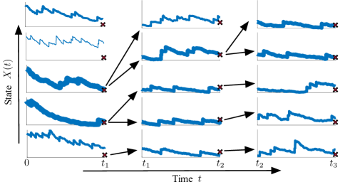
Figure 1: Illustration of the bootstrap filter for a jump-diffusion approximation of a reaction network. The figure shows $M=5$ state particles $\{X_{[t_{n-1},t_{n}]}^{(i)}\}$ for $K=3$ observations, where $i=1,\dots,M$ and $n=1,\dots,K$. The counters $U(t)$ and $V(t)$ are converted into the state variable via Eq. 4. The rows of the figure correspond to the particle index $i$, while the columns are the observation indices $n$. The observations are given as red crosses at the time points $t_{1}<t_{2}<t_{3}$. The line width denotes the particle weight as in Eq. 21. Arrows denote the particle selection phase after resampling. Therefore, particles with a high weight (high line width) are replicated, while others are eliminated, for more details see Section D.1.

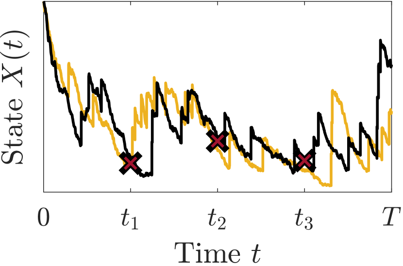
(a)

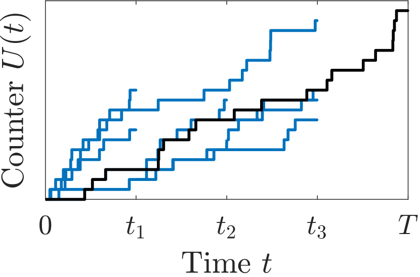
(b)

(c)

Figure 2: Illustration of the backward smoothing procedure. The ground truth latent state trajectory $X(t)$ (yellow line) together with the observations (red crosses) and a smoothing trajectory (black line) are depicted in (2(a)). A smoothing trajectory (black line) of a discrete reaction counter $U(t)$ and a continuous reaction counter $V(t)$ are shown in (2(b)) and (2(c)), respectively. The particles of the bootstrap filter (blue line) represent an empirical distribution for the conditional path measure, see Eq. 22.

In Fig. 1 we show for a small number of particles for the state $X(t)$ and the observations $Y_{1:K}$ an illustration of the bootstrap filter. The corresponding true latent state trajectory is depicted in Fig. 2(a). Figure 2 provides an intuition for the smoothing procedure, where we show in Figs. 2(b) and 2(c) the filter particles of two reaction counters $U(t)\in\mathbb{N}$ and $V(t)\in\mathbb{R}$ together with one backward smoothing trajectory. The backward trajectory is selected according to the empirical distribution in Eq. 22. The corresponding smoothing trajectory sample for the state is depicted in Fig. 2(a).

3.2 Parameter Inference

Having presented a solution to sampling from the full conditional of the state variables as in Eq. 17, we present next a method to sample from the full conditionals as in Eqs. 18 and 20. Therefore, we sample from the conditionals $\operatorname{\mathrm{p}}(\{\phi_{i}\}_{i\in\mathcal{D}}\mid u_{[0,T]},v_{[0,T]},\{\phi_{j}\}_{j\in\mathcal{C}},y_{1:K})$ and $\operatorname{\mathrm{p}}(\{\phi_{j}\}_{j\in\mathcal{C}}\mid u_{[0,T]},w_{[0,T]},\{\phi_{i}\}_{i\in\mathcal{D}},y_{1:K})$ of the slow and fast rate parameters, respectively.

Since computing these conditionals requires in general computing intractable integrals over the parameter space, we next present expressions for the respective unnormalized conditionals. These unnormalized density expressions can be used by mcmc MCMC method like, e.g., the Metropolis-Hastings algorithm or HMC, to yield a Metropolis-within-Gibbs sampling type scheme.

3.2.1 Estimating the Slow Reaction Rate Parameters

First, we want to estimate the reaction rates of the slow reactions, i.e., $\{\Phi_{i}\}_{i\in\mathcal{D}}$. We can find an unnormalized expression for the full conditional $\operatorname{\mathrm{p}}(\{\phi_{i}\}_{i\in\mathcal{D}}\mid u_{[0,T]},v_{[0,T]},\{\phi_{j}\}_{j\in\mathcal{C}},y_{1:K})$ of the slow reactions. For this, we exploit an expression proportional to the path-likelihood $\operatorname{\mathrm{P}}_{U\mid V,\Phi}(\mathrm{d}u_{[0,T]})\coloneqq\operatorname{\mathrm{P}}(\mathrm{d}u_{[0,T]}\mid v_{[0,T]},\{\phi_{i}\}_{i\in\mathcal{D}}),$ for which we use the path measure of the discrete counting process whose details are given in Section 2.1. This yields the following relation

$$\operatorname{\mathrm{p}}(\{\phi_{i}\}_{i\in\mathcal{D}}\mid u_{[0,T]},v_{[0,T]},\{\phi_{j}\}_{j\in\mathcal{C}},y_{1:K})$$

$$\quad\propto\frac{\operatorname{\mathrm{P}}(\mathrm{d}u_{[0,T]}\mid v_{[0,T]},\{\phi_{i}\}_{i\in\mathcal{D}})}{\operatorname{\mathrm{P}}_{\zeta}(\mathrm{d}u_{[0,T]})}\operatorname{\mathrm{p}}(\phi)$$

$$\qquad=\frac{\operatorname{\mathrm{P}}_{U\mid V,\Phi}(\mathrm{d}u_{[0,T]})}{\operatorname{\mathrm{P}}_{\zeta}(\mathrm{d}u_{[0,T]})}\operatorname{\mathrm{p}}(\phi)=D(u_{[0,T]})\operatorname{\mathrm{p}}(\phi),$$

where $\operatorname{\mathrm{P}}_{\zeta}(\mathrm{d}u_{[0,T]})\coloneqq\operatorname{\mathrm{P}}(\zeta_{[0,T]}\in\mathrm{d}u_{[0,T]})$ is the path measure of the multivariate standard-Poisson process $\zeta$ and $D(u_{[0,T]})\coloneqq\frac{\mathrm{d}\operatorname{\mathrm{P}}_{U\mid V,\Phi}}{\mathrm{d}\operatorname{\mathrm{P}}_{\zeta}}(u_{[0,T]})\equiv\frac{\operatorname{\mathrm{P}}_{U\mid V,\Phi}(du_{[0,T]})}{\operatorname{\mathrm{P}}_{\zeta}(\mathrm{d}u_{[0,T]})}$ denotes the Radon-Nikodym derivative between the path-likelihood $\operatorname{\mathrm{P}}_{U\mid V,\Phi}(\mathrm{d}u_{[0,T]})$ and the path measure $\operatorname{\mathrm{P}}_{\zeta}(\mathrm{d}u_{[0,T]})$, see Eq. 9. Hence, using the expression for $D(u_{[0,T]})$ in Eq. 9, we can generate a sample $\{\Phi_{j}\}_{j\in\mathcal{C}}$ of the full conditional in Eq. 20 using the unnormalized density as

$$\operatorname{\mathrm{p}}(\{\phi_{i}\}_{i\in\mathcal{D}}\mid u_{[0,T]},v_{[0,T]},\{\phi_{j}\}_{j\in\mathcal{C}},y_{1:K})$$ (23)

$$\qquad\propto\exp\left(-\int_{0}^{T}\sum_{i\in\mathcal{D}}\kappa_{i}(u(s),v(s))\,\mathrm{d}s\right)$$

$$\qquad\quad\cdot\left(\prod_{i\in\mathcal{D}}\prod_{j=1}^{u_{i}(T)}\kappa_{i}(u(\tau_{i,j}^{-}),v(\tau_{i,j}^{-}))\right)p(\phi).$$

Even though computing the normalization constant in Eq. 23 involves in general an intractable integral over the parameters, we can computationally efficiently sample from the expression using the Metropolis-Hastings algorithm, HMC or extensions like NUTS.

3.2.2 Estimating the Fast Reaction Rate Parameters

Second, we estimate the reaction rates of the fast reactions, i.e., $\{\Phi_{j}\}_{j\in\mathcal{C}}$. Using the model structure, we have the following expression for the unnormalized conditional distribution

$$\operatorname{\mathrm{p}}(\{\phi_{j}\}_{j\in\mathcal{C}}\mid u_{[0,T]},w_{[0,T]},\{\phi_{i}\}_{i\in\mathcal{D}},y_{1:K})$$

$$\propto\operatorname{\mathrm{p}}(y_{1:K}\mid u_{[0,T]},w_{[0,T]},\phi)\operatorname{\mathrm{p}}(\phi).$$

The likelihood can be computed as

$$\operatorname{\mathrm{p}}(y_{1:K}\mid u_{[0,T]},w_{[0,T]},\phi)=\prod_{n=1}^{K}\operatorname{\mathrm{p}}(y_{n}\mid x_{n}),$$

where we compute the state $x_{n}$ using

$$x_{n}=x_{0}+\sum_{i\in\mathcal{D}}u_{i}(t_{n})\mu_{i}+\sum_{j\in\mathcal{C}}v_{j}(t_{n})\mu_{j},$$

with

$$\mathrm{d}v_{j}(t)=$$ (24)

$$\quad\kappa_{j}(u(t),v(t))\,\mathrm{d}t+\sqrt{\kappa_{j}(u(t),v(t))}\,\mathrm{d}w_{j}(t).$$

Hence, we can sample from the full conditional of $\{\Phi_{j}\}_{j\in\mathcal{C}}$ in Eq. 20 using the unnormalized density

$$\operatorname{\mathrm{p}}(\{\phi_{j}\}_{j\in\mathcal{C}}\mid u_{[0,T]},w_{[0,T]},\{\phi_{i}\}_{i\in\mathcal{D}},y_{1:K})$$ (25)

$$\propto\left(\prod_{n=1}^{K}\operatorname{\mathrm{p}}(y_{n}\mid x_{n})\right)\operatorname{\mathrm{p}}(\phi).$$

This concludes the presentation of the proposed blocked Gibbs particle smoother. A pseudo-code summarizing the sampler is given by Section 3.2.2.

[htbp]    input : $Y_{1:K}$: Observation data; $\Phi^{(0)}$: Initial rate parameters; $L$: number of Gibbs samples output : Posterior samples $\{U_{[0,T]}^{(m)},V_{[0,T]}^{(m)},\Phi^{(m)}\}_{m=1}^{L}$ for $m=1$ to $L$ do

2      Sample a smoothing path as in Eq. 22, by SIR particle smoothing, see Section 3.1, i.e., sample

$$U_{[0,T]}^{(m)},V_{[0,T]}^{(m)}\mid\Phi^{(m-1)},Y_{1:K}\sim\operatorname{\mathrm{P}}(\mathrm{d}u_{[0,T]},\mathrm{d}v_{[0,T]}\mid y_{1:K},\phi).$$

Sample the slow reaction rate parameters by drawing from Eq. 23, see Section 3.2.1, i.e., sample

$$\{\Phi_{i}^{(m)}\}_{i\in\mathcal{D}}\mid U_{[0,T]}^{(m)},V_{[0,T]}^{(m)},\{\Phi_{j}^{(m-1)}\}_{j\in\mathcal{C}},Y_{1:K}\sim\operatorname{\mathrm{p}}(\{\phi_{i}\}_{i\in\mathcal{D}}\mid u_{[0,T]},v_{[0,T]},\{\phi_{j}\}_{j\in\mathcal{C}},y_{1:K}).$$

3      Compute the conditional Brownian motions as

$$\mathrm{d}W_{j}^{(m)}(t)=\frac{\mathrm{d}V_{j}^{(m)}(t)-\kappa_{j}(U^{(m)}(t),V^{(m)}(t))\,\mathrm{d}t}{\sqrt{\kappa_{j}(U^{(m)}(t),V^{(m)}(t))}}, \forall j\in\mathcal{C}.$$

4      Sample the fast reaction rate parameters by drawing from Eq. 25, see Section 3.2.2, i.e., sample

$$\{\Phi_{j}^{(m)}\}_{j\in\mathcal{C}}\mid U_{[0,T]}^{(m)},W_{[0,T]}^{(m)},\{\Phi_{i}^{(m)}\}_{i\in\mathcal{D}},Y_{1:K}\sim\operatorname{\mathrm{p}}(\{\phi_{j}\}_{j\in\mathcal{C}}\mid u_{[0,T]},w_{[0,T]},\{\phi_{i}\}_{i\in\mathcal{D}},y_{1:K}).$$

5     

6      end for

Blocked Gibbs Particle Smoothing  

4 A Multi-Scale Birth-Death Process Experiment

In the following, we apply our algorithm to an illustrative example. We consider a birth-death reaction system with two reactions of the form.

$$R_{1}:\rho S\stackrel{{\scriptstyle\phi_{1}}}{{\longrightarrow}}\emptyset,\quad R_{2}:\emptyset\stackrel{{\scriptstyle\phi_{2}}}{{\longrightarrow}}\eta S,$$ (26)

with stoichiometries $\rho\in\mathbb{N}$ and $\eta\in\mathbb{N}$. In this example, $R_{1}$ is considered to be a fast reaction and is therefore modeled by a diffusion approximation, while a discrete state Markov chain updating scheme is kept for the slow reaction $R_{2}$. Hence, the sets of fast and slow reactions, the stoichiometries, and the respective change vectors are given by

$$\begin{gathered}\begin{aligned} &\mathcal{C}=\{1\},&&\mathcal{D}&=\{2\},\end{aligned}\\ \begin{aligned} &\underline{\mu}_{1}=\rho,&&\bar{\mu}_{1}=0\,\unit{},&&&\mu_{1}=-\rho,\\ &\underline{\mu}_{2}=0\,\unit{},&&\bar{\mu}_{2}=\eta,&&&\mu_{2}=\eta,\end{aligned}\end{gathered}$$

where we assume a substrate stoichiometry of $\rho=1\,\unit{}$ and product stoicheometry of $\eta=10\,\unit{}$. The system’s state vector at time $t\geq 0$ is represented by $X(t)\in\mathbb{R}$. We divide the reaction counters of the system into two groups, i.e., $N(t)=(U(t),V(t))^{\top}$, with $U(t)\in\mathbb{Z}_{\geq 0}$ and $V(t)\in\mathbb{R}$ representing the firing number of slow and fast reactions until time $t>0$, respectively. This yields the state vector of the system as

$$X(t)=X(0)+\eta U(t)-\rho V(t),$$ (27)

Where we assume that the state of the system is deterministically initialized as $X(0)=60\,\unit{}$. The corresponding reaction counters of the system obey the following equations.

$$\begin{aligned} V(t)=&\int_{0}^{t}\kappa_{1}(U(s),V(s))\,\mathrm{d}s\\ &{}+W\left(\int_{0}^{t}\kappa_{1}(U(s),V(s))\,\mathrm{d}s\right),\end{aligned}$$ (28)

$$\begin{aligned} U(t)=\zeta\left(\int_{0}^{t}\kappa_{2}(U(s),V(s))\,\mathrm{d}s\right),\end{aligned}$$ (29)

and by definition we have $U(0)=V(0)=0$. The propensity functions above to follow the law of mass action kinetics as

$$\begin{multlined}\kappa_{1}(u,v)=\gamma_{1}(X(0)+\eta u-\rho v)\\ =\phi_{1}\frac{X(0)+\eta u-\rho v}{\rho},\end{multlined}\kappa_{1}(u,v)=\gamma_{1}(X(0)+\eta u-\rho v)\\ =\phi_{1}\frac{X(0)+\eta u-\rho v}{\rho},$$ (30)

$$\begin{multlined}\kappa_{2}(u,v)=\gamma_{2}(X(0)+\eta u-\rho v)=\phi_{2},\end{multlined}\kappa_{2}(u,v)=\gamma_{2}(X(0)+\eta u-\rho v)=\phi_{2},$$

and the latent rates are set to $\phi_{1}=2\,\unit{\per}$ and $\phi_{2}=4\,\unit{\per}$, hence $\phi=(2\,\unit{\per},4\,\unit{\per})^{\top}$. Therefore, the HME in Eq. 7 computes to

$$\begin{multlined}\partial_{t}\operatorname{\mathrm{p}}(u,v,t\mid\mathcal{H})=\phi_{1}\frac{X(0)+\eta u-\rho v}{\rho}\\ \cdot\left(\frac{1}{2}\partial_{v}^{2}\operatorname{\mathrm{p}}(u,v,t\mid\mathcal{H})-\partial_{v}\operatorname{\mathrm{p}}(u,v,t\mid\mathcal{H})\right)\\ -\phi_{1}(\partial_{v}\operatorname{\mathrm{p}}(u,v,t\mid\mathcal{H})-\operatorname{\mathrm{p}}(u,v,t\mid\mathcal{H}))\\ +\phi_{2}(\operatorname{\mathrm{p}}(u-1,v,t\mid\mathcal{H})-\operatorname{\mathrm{p}}(u,v,t\mid\mathcal{H})),\end{multlined}\partial_{t}\operatorname{\mathrm{p}}(u,v,t\mid\mathcal{H})=\phi_{1}\frac{X(0)+\eta u-\rho v}{\rho}\\ \cdot\left(\frac{1}{2}\partial_{v}^{2}\operatorname{\mathrm{p}}(u,v,t\mid\mathcal{H})-\partial_{v}\operatorname{\mathrm{p}}(u,v,t\mid\mathcal{H})\right)\\ -\phi_{1}(\partial_{v}\operatorname{\mathrm{p}}(u,v,t\mid\mathcal{H})-\operatorname{\mathrm{p}}(u,v,t\mid\mathcal{H}))\\ +\phi_{2}(\operatorname{\mathrm{p}}(u-1,v,t\mid\mathcal{H})-\operatorname{\mathrm{p}}(u,v,t\mid\mathcal{H})),$$

see Appendix E. Further, we assume a Gaussian observation model for the state as

$$Y_{n}\mid X_{n}\sim\operatorname{\mathcal{N}}(y_{n}\mid x_{n},\sigma^{2}),$$ (31)

where we set the standard deviation to $\sigma=4\,\unit{}$. The state $X(t)$ is observed at $K=50$ time points $\{t_{n}\}_{n=1}^{K}$, which are uniformly distributed in the time interval $[0,T]$, with $T=10\,\unit{}$. The resulting latent ground-truth trajectories and the observations are depicted in Fig. 3. For the numerical simulation of the diffusion process $V(t)$, we use throughout this paper, if not stated otherwise, a stochastic Runge-Kutta method [Rößler, 2010], where we set the integration step to $10^{-2}\,\unit{}$, utilizing torchsde [Li et al., 2020] within the PyTorch framework [Paszke et al., 2019]. For the Markov jump process (MJP) $U(t)$, we utilize the Doob-Gillespie algorithm [Doob, 1945], see, e.g., Wilkinson [2006].

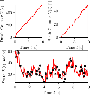
Figure 3: Illustration of the ground-truth realization. The trajectories correspond to a static partitioning into slow and fast reaction channels. Upper Left Panel: Realization of the reaction counter $U$, modeled as ctmc CTMC, which corresponds to the dynamics of the reaction counter of the slow reaction $R_{2}$ given in Eq. 29. Upper Right Panel: Realization of the reaction counter $V$, modeled using a diffusion approximation, which corresponds to the dynamics of the reaction counter of the fast reaction $R_{1}$ given in Eq. 28. Lower Panel: The corresponding realization of the state $X$ as given in Eq. 27 and the discrete-time observations $Y_{1:K}$ as in Eq. 31 depicted as crosses.

Posterior Inference

We sample from the posterior

$$X_{[0,T]},\Phi\mid Y_{1:K}\sim\operatorname{\mathrm{P}}(\mathrm{d}x_{[0,T]},\mathrm{d}\phi\mid y_{1:K}),$$

by using the proposed blocked Gibbs particle smoother, as in Section 3.2.2. We perform $1300$ iterations, where we discard the first $300$ samples to adjust for burn-in of the sampler, yielding $L=1000$ posterior samples. In each step of the sampler, we run the SIR particle smoothing step with $M=5000$ particles. To adjust for particle degeneracy, we use systematic resampling inside the particle filtering step and use a minimum effective particle ratio of $\alpha=0.5$ for the resampling threshold, for details see Section D.1. We choose an independent prior distribution for the rate parameters $\{\Phi_{i}\}_{i=1}^{2}$, which is parameterized as

$$\operatorname{\mathrm{p}}(\phi_{1},\phi_{2})=\prod_{i=1}^{2}\operatorname{\mathrm{Gam}}(\phi_{i}\mid a,b).$$

We choose a vague prior distribution by specifying a small shape and rate hyper-parameter, i.e., we use $a=10^{-6}$ and $b=10^{-6}\,\unit{}$, respectively. This yields a vague scale prior that is approximately a flat improper prior distribution, as the gamma distribution with small shape and rate parameters is roughly the reciprocal distribution (or log-uniform distribution) on the positive reals, i.e.,

$$\prod_{i=1}^{2}\operatorname{\mathrm{Gam}}(\phi_{i}\mid 10^{-6},10^{-6})$$

$$\approx\prod_{i=1}^{2}\operatorname{\mathrm{LogUniform}}(\phi_{i}){\propto}(\phi_{1}\phi_{2})^{-1}.$$

Therefore, we have a sensible prior that is an improper uniform prior on the real numbers in the log-domain, i.e.,

$$\operatorname{\mathrm{p}}(\log\phi_{i})\approx\operatorname{\mathrm{Uniform}}(\log\phi_{i})\propto 1 i=1,2.$$

For sampling from the unnormalized full-conditionals of the parameters in Eqs. 23 and 25, we use the No-U-Turn Sampler (NUTS) of Hoffman et al. [2014], by implementing our system in the probabilistic programming language Pyro [Bingham et al., 2019]. The hyper-parameters are set to the default values in Pyro. In each Gibbs step over the parameters, we perform $100$ warmup steps within NUTS for burn-in. In the model for the unnormalized full-conditional of the fast reaction, see Eq. 25, we compute the reparameterization in Eq. 19 using the step-size of $10^{-2}\,\unit{}$, that is consistent to the particle simulation step size of the stochastic Runge-Kutta integrator. Subsequently, using the Euler-Maruyama method with the same step size, we integrate the resulting reparameterization in Eq. 24.

4.1 Results

The results for the inference of the partially observed multi-scale birth death reaction network using the posterior samples $\{X^{(m)}_{[0,T]},\Phi^{(m)}\}_{m=1}^{L}$ are depicted in Figs. 4, 5 and 6.

In Fig. 4, we show the ground-truth latent state trajectory, together with the observations. The posterior distribution is summarized in the graphic by the posterior mean estimate

$$\hat{X}(t)=\operatorname{\mathsf{E}}\left[X(t)\nonscript\;\middle|\nonscript\;Y_{1:K}\right]\approx\frac{1}{L}\sum_{m=1}^{L}X^{(m)}(t)$$

and the time-point-wise posterior state marginals

$$\operatorname{\mathrm{p}}(x,t\mid y_{1:K})\approx\frac{1}{L}\sum_{m=1}^{L}\delta(X^{(m)}(t)-x).$$

We visualize these in Fig. 4 by the $5\%\backslash 95\%-$ and $25\%\backslash 75\%-$quantile regions and by a kernel density approximation $\hat{\operatorname{\mathrm{p}}}(x,t)\approx\operatorname{\mathrm{p}}(x,t\mid y_{1:K})$, i.e.,

$$\hat{\operatorname{\mathrm{p}}}(x,t)=\frac{1}{L}\sum_{m=1}^{L}\mathcal{K}(X^{(m)}(t)-x),$$

using a scaled Gaussian kernel $\mathcal{K}(x)=\operatorname{\mathcal{N}}(x\mid 0,h^{2})$, with bandwidth $h$.

In both plots, we observe that the state posterior tracks the ground truth, while the posterior uncertainty increases between observation time points. Note that due to the observation variance $\sigma^{2}$, the posterior variance never shrinks exactly to zero.

In Fig. 5, we visualize the results for the parameter estimation by the marginal posterior.

$$\operatorname{\mathrm{p}}(\phi_{1},\phi_{2}\mid y_{1:K})\approx\frac{1}{L}\sum_{m=1}^{L}\delta(\Phi_{1}^{(m)}-\phi_{1})\delta(\Phi_{2}^{(m)}-\phi_{2}).$$

We show the ground-truth parameters together with the posterior samples $\{\Phi^{(m)}\}_{m=1}^{L}$. The marginal parameter posterior is visualized by a kernel density estimate $\hat{\operatorname{\mathrm{p}}}(\phi_{1},\phi_{2})\approx\operatorname{\mathrm{p}}(\phi_{1},\phi_{2}\mid y_{1:K})$, i.e.,

$$\hat{\operatorname{\mathrm{p}}}(\phi_{1},\phi_{2})=\hat{\operatorname{\mathrm{p}}}(\phi)=\frac{1}{L}\sum_{m=1}^{L}\mathcal{K}(\Phi^{(m)}-\phi).$$

Additionally, we show high-density regions for both the prior $\operatorname{\mathrm{p}}(\phi_{1},\phi_{2})$ and marginal parameter posterior distribution $\operatorname{\mathrm{p}}(\phi_{1},\phi_{2}\mid y_{1:K})$, depicted using the isolines of the $5\%-$, $25\%-$ $75\%-$ and $95\%-$quantiles.

We see that the posterior concentrates around the ground-truth value. Consequently, the isolines are shifting from the prior to the posterior density. However, the parameters cannot be identified due to the limited number of observations $K$ and the observation variance $\sigma^{2}$. As such, the parameter posterior samples lie on an ellipse, visualized by the kernel density estimate. This is a known effect in the context of parameter inference in chemical reaction networks, see, e.g., Wilkinson [2006].

Finally, Fig. 6 shows the observations $Y_{1:K}$ and the posterior predictive distribution

$$\operatorname{\mathrm{p}}(y^{\ast},t\mid y_{1:K}) =\int\operatorname{\mathrm{p}}(y^{\ast}\mid x)\operatorname{\mathrm{p}}(x,t\mid y_{1:K})\,\mathrm{d}x$$

$$=\operatorname{\mathsf{E}}\left[\operatorname{\mathrm{p}}(y^{\ast}\mid X(t))\nonscript\;\middle|\nonscript\;Y_{1:K}\right]$$

$$\approx\frac{1}{L}\sum_{m=1}^{L}\operatorname{\mathrm{p}}(y^{\ast}\mid X^{(m)}(t))$$

$$\quad=\frac{1}{L}\sum_{m=1}^{L}\operatorname{\mathcal{N}}(y^{\ast}\mid X^{(m)}(t),\sigma^{2}).$$

From Fig. 6 we assert that the posterior predictive distribution

$$Y^{\ast}(t)\mid Y_{1:K}\sim\operatorname{\mathrm{p}}(y^{\ast},t\mid y_{1:K})$$

over hypothetical observations $Y^{\ast}(t)$ can explain the given observations $Y_{1:K}$.

Figure 4: Posterior state inference for the multi-scale birth-death process. The plots visualize the ground truth state trajectory, the observations (white crosses), the posterior mean, and the marginal state posterior $\operatorname{\mathrm{p}}(x,t\mid y_{1:K})$. The figure background color indicates a kernel density estimate for the marginal state posterior and the $5\%\backslash 95\%$ (solid line) and $25\%\backslash 75\%$ (dashed line) posterior quantiles.

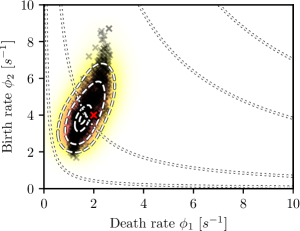
Figure 5: Parameter inference for the multi-scale birth-death process, with only $K=50$ observation points. The graphic shows the ground-truth parameter and the marginal parameter posterior $\operatorname{\mathrm{p}}(\phi_{1},\phi_{2}\mid y_{1:K})$. The marginal parameter posterior is visualized by the posterior parameter samples, and a kernel density estimate is shown in the background. The isolines visualize high-density regions for the parameter prior distribution $\operatorname{\mathrm{p}}(\phi_{1},\phi_{2})\propto(\phi_{1}\phi_{2})^{-1}$ (dotted white line) and the marginal parameter posterior (dashed white line).

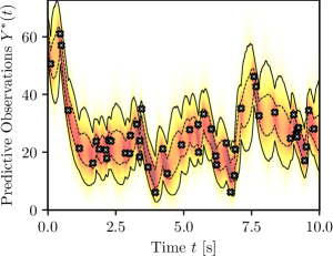
Figure 6: Posterior predictive distribution for the multi-scale birth-death process. The background shows the posterior predictive distribution $\operatorname{\mathrm{p}}(y^{\ast},t\mid y_{1:K})$ obtained using the posterior samples of the Gibbs sampling procedure. The lines indicate the $5\%\backslash 95\%$ (solid line) and $25\%\backslash 75\%$ (dashed line) posterior quantiles. The given observations $Y_{1:K}$ are shown as white crosses.

Additionally, to the presented setting, we provide a comparison for different number of observations $K$ and different observation noise parameters $\sigma$ in Tables 1, 2 and 3.

In Table 1, we give the means of the posterior samples $\{\Phi^{(m)}\}_{m=1}^{L}$ together with the posterior standard deviations for the ground-truth setting with parameters $(\phi_{1},\phi_{2})=(2,4)^{\top}$ in terms of the different number of observations $K$ and the different observation noise standard deviation $\sigma$. The results show that the performance of the algorithm increases proportionally with the increase of the number of observations $K$ and the decrease of the observation noise standard deviation $\sigma$. For fixed values of $\sigma$, the increase in the number of observations $K$ gives better results. It must also be noted that for a fixed number of observations $K$, the increase in the observation noise standard deviation $\sigma$ leads to wider ranges for the posterior mean that brings along uncertainty. However, for very large noise and a low number of observations, the parameters get more and more unidentifiable.

	Posterior parameter mean $\pm$ standard deviation ($\unit{\per}$)
	$K=100$	$K=50$	$K=10$
$\sigma=1\,\unit{}$	$(1.90,4.44)\pm(0.10,0.72)$	$(1.70,4.27)\pm(0.12,0.77)$	$(0.59,1.39)\pm(0.13,0.55)$
$\sigma=2\,\unit{}$	$(2.16,4.02)\pm(0.30,0.85)$	$(2.78,5.66)\pm(0.36,1.13)$	$(2.08,3.72)\pm(0.50,1.26)$
$\sigma=4\,\unit{}$	$(1.06,2.77)\pm(0.11,0.66)$	$(1.55,2.24)\pm(0.37,0.78)$	$(2.69,5.78)\pm(0.84,2.20)$
$\sigma=8\,\unit{}$	$(2.12,3.93)\pm(0.52,1.22)$	$(1.63,4.45)\pm(0.45,1.52)$	$(0.20,0.05)\pm(0.06,0.16)$

Table 1: Posterior means and ($\pm$) standard deviations for the parameters $(\phi_{1},\phi_{2})=(2,4)^{\top}$, depending on the number of observations $K$ and the observation noise standard deviation $\sigma$.

In Table 2, we compare the mean of the effective number of particles $\bar{M}_{\text{EPS}}$ and the mean of the unique number of particles $\bar{M}_{\text{unique}}$ after resampling with $M=5000$ particles for different number of observations $K$ and for different observation noise standard deviations $\sigma$. The outcomes validate that enough particles always survive after resampling. It is visible that $\bar{M}_{\text{EPS}}$ decreases with the increase of the observation noise standard deviation $\sigma$ and the increase in the number of observation $K$. This is caused by the increase in variance of the system dynamics. Another result that can be seen from the table is that for a fixed number of observations $K$, the mean of the unique particles $\bar{M}_{\text{unique}}$ increase parallel with the increase in the observation noise standard deviation $\sigma$. While for a fixed observation noise standard deviation $\sigma$, the mean of the unique particles $\bar{M}_{\text{unique}}$ increase with the number of observations $K$.

	$K=100$			$K=50$			$K=10$
	$\bar{M}_{\text{EPS}}$	$\bar{M}_{\text{unique}}$		$\bar{M}_{\text{EPS}}$	$\bar{M}_{\text{unique}}$		$\bar{M}_{\text{EPS}}$	$\bar{M}_{\text{unique}}$
$\sigma=1\,\unit{}$	$4644$	$2138$		$4806$	$1662$		$4988$	$1542$
$\sigma=2\,\unit{}$	$4389$	$2960$		$4704$	$2224$		$4934$	$1887$
$\sigma=4\,\unit{}$	$4199$	$3612$		$4251$	$3494$		$4744$	$2524$
$\sigma=8\,\unit{}$	$4057$	$4164$		$4072$	$3918$		$4087$	$4569$

Table 2: The Mean of the effective number of particles $\bar{M}_{\text{EPS}}$ and the mean of the unique number of particles $\bar{M}_{\text{unique}}$ after resampling used for the particle filtering with $M=5000$ particles, depending on the number of observations $K$ and the observation noise standard deviation $\sigma$.

Finally, in Table 3, we compare the root mean square error $\text{RMSE}=\sqrt{\frac{1}{T}\int_{0}^{T}(\hat{X}(t)-X(t))^{2}\,\mathrm{d}t}$ of the state estimate $\hat{X}(t)$ for different number of observations $K$ and for different observation noise standard deviations $\sigma$. It is discernible that for fixed values of the observation noise standard deviation $\sigma$, RMSE decreases with the increase in the number of observation $K$. Also, the decrease in the observation noise standard deviation $\sigma$ for a fixed number of observations $K$ results in a decrease in the RMSE. Note, that the presented RMSE value, is only given for one experiment.

	RMSE ($\unit{}$)
	$K=100$	$K=50$	$K=10$
$\sigma=1\,\unit{}$	$3.84$	$4.91$	$9.69$
$\sigma=2\,\unit{}$	$3.77$	$4.59$	$5.87$
$\sigma=4\,\unit{}$	$5.55$	$4.12$	$10.58$
$\sigma=8\,\unit{}$	$5.47$	$6.62$	$9.06$

Table 3: Root mean square error $\text{RMSE}=\sqrt{\frac{1}{T}\int_{0}^{T}(\hat{X}(t)-X(t))^{2}\,\mathrm{d}t}$ of the posterior mean state estimate $\hat{X}(t)$, depending on the number of observations $K$ and the observation noise standard deviation $\sigma$.

5 Conclusion

By exploiting a hybrid modeling approach to BRNs we presented a coherent framework for fast and tractable Bayesian inference for partially observed reaction networks exhibiting a multi-scale behavior. The proposed blocked Gibbs particle smoothing algorithm overcomes the obstacles posed by the derived intractable equations of exact posterior inference. This is achieved by performing separate blocked Gibbs steps for state and parameter inference in the BRNs modeled by a jump-diffusion approximation. Efficient inference is accomplished by utilizing a particle-based forward-filtering backward-smoothing algorithm and mcmc MCMC-based sampler for state and parameter inference, respectively. The presented numerical case study exemplifies the algorithm by showing its applicability to an illustrative setup of a birth-death process, which exhibits a multi-scale behavior.

As a possible future work, we think that our algorithm can be the base for new inference algorithms exploiting the jump-diffusion approximation for BRN models. For example, it is known that a naive application of a particle-based posterior approximation suffers as the state dimension increases. Therefore, in order take to make the proposed algorithm more applicable in such settings, a possible future work includes the improvement of the state inference procedure, e.g., by finding an improved proposal distribution for the underlying particle approximation. Additionally, we think that the ideas presented in this work might be of use in other contexts for state and parameter inference, where the underlying model exhibits a multi-scale behavior, well beyond BRNs.

Acknowledgments Derya Altıntan acknowledges support from the German Academic Exchange Service DAAD, Program no: 57552334 Grant no. 91527068. Additionally, this work has been funded by the German Research Foundation (DFG) as part of the project B4 within the Collaborative Research Center (CRC) 1053 – MAKI.

Appendix A Notation

In this section, we present some basic notation used throughout this paper.

All random variables and their realizations are represented by upper-case symbols, e.g., $Z$, and lower-case symbols, e.g., $z$, respectively.

We denote by $e_{j}$ and $\bar{e}_{j}$ the $l$-dimensional and the $(r-l)$-dimensional unit vectors with $1$ in the $j$th component and $0$ in all other components, respectively.

Any sequence $z_{a:b}$, with $a\in\mathbb{N}$, $b\in\mathbb{N}$ and $a<b$ represents the vector

$$z_{a:b}\coloneqq(z_{a},z_{a+1},\dots,z_{b-1},z_{b})^{\top}.$$

For a stochastic process $Z$, we write $Z_{[a,b]}$ representing the path

$$Z_{[a,b]}\coloneqq\{Z(t):\,t\in[a,b]\}.$$

We denote by

$$Z_{i}=Z(t_{i}),$$

with $i\in\mathbb{N}$ a random variable $Z_{i}$ at an observation point $t_{i}$ of a stochastic process $Z$, with the observation times $t_{1}<t_{2}<t_{3}<\dots$ and we define $t_{0}\coloneqq 0$.

For the probability measure of a random variable $Z$, we use the shorthand

$$\operatorname{\mathrm{P}}(\mathrm{d}z)\coloneqq\operatorname{\mathrm{P}}(Z\in\mathrm{d}z)$$

that is for a set $\mathcal{A}$ we have $\operatorname{\mathrm{P}}(Z\in\mathcal{A})=\int_{\mathcal{A}}\operatorname{\mathrm{P}}(\mathrm{d}z)$. For the probability mass function of a time-dependent discrete-valued variable $U(t)$ at time $t$ we write

$$\operatorname{\mathrm{p}}(u,t)\coloneqq\operatorname{\mathrm{P}}(U(t)=u).$$

For the probability density function of a time-dependent continuous-valued random variable $V(t)$ at time $t$, we use

$$\operatorname{\mathrm{p}}(v,t)\coloneqq\partial_{v}\operatorname{\mathrm{P}}(V(t)\leq v).$$

where ?$\leq$? and ?$\partial_{v}$? denote element-wise operation. For the joint probability density function with a discrete random variable $U(t)$ and a continuous random variable $V(t)$ at time $t$, we use

$$\operatorname{\mathrm{p}}(u,v,t)\coloneqq\partial_{v}\operatorname{\mathrm{P}}(V(t)\leq v,U(t)=u).$$

with $p:\mathbb{N}^{l}\times\mathbb{R}^{(A-l)}_{\geq 0}\longrightarrow\mathbb{R}_{\geq 0}$. For the joint distribution, we have

$$\operatorname{\mathrm{p}}(u,v,t)=\operatorname{\mathrm{p}}(v\mid u,t)\operatorname{\mathrm{p}}(u,t),$$

where the conditional density is given as

$$\operatorname{\mathrm{p}}(v\mid u,t)\coloneqq\partial_{v}\operatorname{\mathrm{P}}(V(t)\leq v\mid U(t)=u).$$

For the conditional density at two different time points, we use

$$\operatorname{\mathrm{p}}(u,v,t\mid u^{\prime},v^{\prime},t^{\prime})\coloneqq$$

$$\partial_{v}\operatorname{\mathrm{P}}(V(t)\leq v,U(t)=u\mid V(t^{\prime})=v^{\prime},U(t^{\prime})=u^{\prime}).$$

Appendix B Reaction Network Model

B.1 Proof of Theorem 1

Proof: Following Altıntan and Koeppl [2020] and Pawula [1967], we write

$$\partial_{t}\operatorname{\mathrm{p}}(u,v,t\mid\mathcal{H})$$

$$=\sum_{u^{\prime}\in\mathcal{U}}\lim_{h\rightarrow 0}\frac{1}{h}[\operatorname{\mathrm{p}}(u,t+h\mid u^{\prime},v,t,\mathcal{H})-\delta_{uu^{\prime}}]$$

$$\;\cdot\operatorname{\mathrm{p}}(u^{\prime},v,t\mid\mathcal{H})+\sum_{a_{1},a_{2},\dots,a_{r-l}=1}^{\infty}\left(\prod_{i=1}^{r-l}\frac{(-1)^{a_{i}}\frac{\partial^{a_{i}}}{\partial v_{i}^{a_{i}}}}{a_{i}!}\right)$$

$$\quad\begin{multlined}\cdot\lim_{h\rightarrow 0}\frac{1}{h}\operatorname{\mathsf{E}}\left[\prod_{i=1}^{r-l}\{V_{i}(t+h)-V_{i}(t)\}^{a_{i}}\nonscript\;\middle|\nonscript\;U(t)=u,\right.\\ \left.V(t)\leq v,U(t+h)=u,\mathcal{H}\right],\end{multlined}\cdot\lim_{h\rightarrow 0}\frac{1}{h}\operatorname{\mathsf{E}}\left[\prod_{i=1}^{r-l}\{V_{i}(t+h)-V_{i}(t)\}^{a_{i}}\nonscript\;\middle|\nonscript\;U(t)=u,\right.\\ \left.V(t)\leq v,U(t+h)=u,\mathcal{H}\right],$$

with $\operatorname{\mathsf{E}}\left[V(t)\nonscript\;\middle|\nonscript\;u\right]={\int_{\mathbb{R}_{\geq 0}^{r-l}}}v\>\operatorname{\mathrm{p}}(v\mid u,t,\mathcal{H})\,\mathrm{d}v$.

It is proven in Pawula [1967], that for $\sum_{i=1}^{r-l}a_{i}\geq 3$ we have

$$\begin{multlined}\lim_{h\rightarrow 0}\frac{1}{h}\operatorname{\mathsf{E}}\left[\prod_{i=1}^{r-l}\{V_{i}(t+h)-V_{i}(t)\}^{a_{i}}\nonscript\;\middle|\nonscript\;U(t)=u,\right.\\ \left.V(t)\leq v,U(t+h)=u,\mathcal{H}\right]=0.\end{multlined}\lim_{h\rightarrow 0}\frac{1}{h}\operatorname{\mathsf{E}}\left[\prod_{i=1}^{r-l}\{V_{i}(t+h)-V_{i}(t)\}^{a_{i}}\nonscript\;\middle|\nonscript\;U(t)=u,\right.\\ \left.V(t)\leq v,U(t+h)=u,\mathcal{H}\right]=0.$$

This result gives us

$$\partial_{t}\operatorname{\mathrm{p}}(u,v,t\mid\mathcal{H})$$

$${}=\sum_{u^{\prime}\in\mathcal{U}}\lim_{h\rightarrow 0}\frac{1}{h}[\operatorname{\mathrm{p}}(u,t+h\mid u^{\prime},v,t,\mathcal{H})-\delta_{uu^{\prime}}]$$

$$\quad\cdot\operatorname{\mathrm{p}}(u^{\prime},v,t\mid\mathcal{H})-\sum_{j=1}^{r-l}\partial_{v_{j}}[\Lambda_{j}\operatorname{\mathrm{p}}(u,v,t\mid\mathcal{H})]$$

$$\quad+\frac{1}{2}\sum_{i,j=1}^{r-l}\partial_{v_{i}}\partial_{v_{j}}[\Lambda_{ij}\operatorname{\mathrm{p}}(u,v,t\mid\mathcal{H})],$$

where

$$\begin{multlined}\Lambda_{j}=\lim_{h\rightarrow 0}\frac{1}{h}\operatorname{\mathsf{E}}\left[(V_{j}(t+h)-V_{j}(t))\nonscript\;\middle|\nonscript\;U(t)=u,\right.\\ \left.V(t)\leq v,U(t+h)=u,\mathcal{H}\right]\end{multlined}\Lambda_{j}=\lim_{h\rightarrow 0}\frac{1}{h}\operatorname{\mathsf{E}}\left[(V_{j}(t+h)-V_{j}(t))\nonscript\;\middle|\nonscript\;U(t)=u,\right.\\ \left.V(t)\leq v,U(t+h)=u,\mathcal{H}\right]$$

$$\begin{multlined}\Lambda_{ij}=\lim_{h\rightarrow 0}\frac{1}{h}\operatorname{\mathsf{E}}\left[\{V_{i}(t+h)-V_{i}(t)\}\{V_{j}(t+h)\right.\\ \left.-V_{j}(t)\}\nonscript\;\middle|\nonscript\;U(t)=u,V(t)\leq v,U(t+h)=u,\mathcal{H}\right].\end{multlined}\Lambda_{ij}=\lim_{h\rightarrow 0}\frac{1}{h}\operatorname{\mathsf{E}}\left[\{V_{i}(t+h)-V_{i}(t)\}\{V_{j}(t+h)\right.\\ \left.-V_{j}(t)\}\nonscript\;\middle|\nonscript\;U(t)=u,V(t)\leq v,U(t+h)=u,\mathcal{H}\right].$$

In the presented jump-diffusion approximation, fast reactions always fire. This means that between two successive firing times $\tau_{1}$ and $\tau_{2}$ of slow reactions, the reaction counter of a fast reaction satisfies the following diffusion process

$$V(t) =V(\tau_{1})+\sum_{j\in\mathcal{C}}\left(\int_{\tau_{1}}^{t}\kappa_{j}(U(s),V(s))\,\mathrm{d}s\right)\bar{e}_{j}$$ (32)

$$+\sum_{j\in\mathcal{C}}W_{j}\left(\int_{\tau_{1}}^{t}\kappa_{j}(U(s),V(s))\,\mathrm{d}s\right)\bar{e}_{j}.$$

Based on these results, we obtain $\Lambda_{j}$, $\Lambda_{ij}$ as follows [Gillespie, 1980, Kampen, 1982]

$$\Lambda_{j}=\sum_{k\in\mathcal{C}}\bar{e}_{jk}\kappa_{k}(u,v),\quad\Lambda_{ij}=\sum_{k\in\mathcal{C}}\bar{e}_{ik}\bar{e}_{jk}\kappa_{k}(u,v),$$

which in turn gives

$$\partial_{t}\operatorname{\mathrm{p}}(u,v,t\mid\mathcal{H})$$ (33)

$$=\sum_{u^{\prime}\in\mathcal{U}}\lim_{h\rightarrow 0}\frac{1}{h}[\operatorname{\mathrm{p}}(u,t+h\mid u^{\prime},v,t,\mathcal{H})-\delta_{uu^{\prime}}]$$

$${}\quad\cdot\operatorname{\mathrm{p}}(u^{\prime},v,t\mid\mathcal{H})-\sum_{j\in\mathcal{C}}\partial_{v_{j}}(\kappa_{j}(u,v)\operatorname{\mathrm{p}}(u,v,t\mid\mathcal{H}))$$

$$\quad+\frac{1}{2}\sum_{j\in\mathcal{C}}\partial_{v_{j}}^{2}(\kappa_{j}(u,v)\operatorname{\mathrm{p}}(u,v,t\mid\mathcal{H})).$$

Now, let us focus on the first summation on the right-hand side of the Eq. 33. Using $\delta_{uu}=1$, gives the following equality

$$\sum_{u^{\prime}\in\mathcal{U}}\lim_{h\rightarrow 0}\frac{1}{h}[\operatorname{\mathrm{p}}(u,t+h\mid u^{\prime},v,t,\mathcal{H})-\delta_{uu^{\prime}}]$$

$$=\sum_{\begin{subarray}{c}u\neq u^{\prime}\\ u^{\prime}\in\mathcal{U}\end{subarray}}\lim_{h\rightarrow 0}\frac{1}{h}[\operatorname{\mathrm{p}}(u,t+h\mid u^{\prime},v,t,\mathcal{H})]$$

$$+\lim_{h\rightarrow 0}\frac{1}{h}[\operatorname{\mathrm{p}}(u,t+h\mid u,v,t,\mathcal{H})-1].$$

Further, by exploiting the complement rule we write

$$\lim_{h\rightarrow 0}\frac{1}{h}[\operatorname{\mathrm{p}}(u,t+h\mid u,v,t,\mathcal{H})-1]$$

$$=\lim_{h\rightarrow 0}\frac{1}{h}[-\sum_{\begin{subarray}{c}u\neq u^{\prime}\\ u^{\prime}\in\mathcal{U}\end{subarray}}\operatorname{\mathrm{p}}(u^{\prime},t+h\mid u,v,t,\mathcal{H})].$$

Then, we get

$$\sum_{u^{\prime}\in\mathcal{U}}\lim_{h\rightarrow 0}\frac{1}{h}[\operatorname{\mathrm{p}}(u,t+h\mid u^{\prime},v,t,\mathcal{H})-\delta_{uu^{\prime}}]$$

$$=\sum_{\begin{subarray}{c}u\neq u^{\prime}\\ u^{\prime}\in\mathcal{U}\end{subarray}}\Big{(}\lim_{h\rightarrow 0}\frac{1}{h}[\operatorname{\mathrm{p}}(u,t+h\mid u^{\prime},v,t,\mathcal{H})]$$

$$-\lim_{h\rightarrow 0}\frac{1}{h}[\operatorname{\mathrm{p}}(u^{\prime},t+h,\mid u,v,t,\mathcal{H})]\Big{)}.$$

If $U(t)=u$, then one firing of reaction $R_{i}$, $i\in\mathcal{D}$, will jump to the state $u^{\prime}=u+e_{i}$ which gives

$$\lim_{h\rightarrow 0}\frac{1}{h}[\operatorname{\mathrm{p}}(u^{\prime},t+h,\mid u,v,t,\mathcal{H})]=\kappa_{i}(u,v),$$

and similarly for $u^{\prime}=u-e_{i}$

$$\lim_{h\rightarrow 0}\frac{1}{h}[\operatorname{\mathrm{p}}(u,t+h,\mid u^{\prime},v,t,\mathcal{H})]=\kappa_{i}(u-e_{i},v).$$

Substitution these results into Eq. 33 give us

$$\partial_{t}\operatorname{\mathrm{p}}(u,v,t\mid\mathcal{H})=\mathscr{A}\operatorname{\mathrm{p}}(u,v,t\mid\mathcal{H}),$$

where $\mathscr{A}(\cdot)=\mathscr{D}(\cdot)+\mathscr{C}(\cdot)$ defined as

$$\mathscr{D}\operatorname{\mathrm{p}}(u,v,t\mid\mathcal{H}) =\sum_{i\in\mathcal{D}}\left(\kappa_{i}(u-e_{i},v)\operatorname{\mathrm{p}}(u-e_{i},v,t\mid\mathcal{H})\right.$$

$$\left.-\kappa_{i}(u,v)\operatorname{\mathrm{p}}(u,v,t\mid\mathcal{H})\right)$$

$$\mathscr{C}\operatorname{\mathrm{p}}(u,v,t\mid\mathcal{H}) =-\sum_{j\in\mathcal{C}}\partial_{v_{j}}(\kappa_{j}(u,v)\operatorname{\mathrm{p}}(u,v,t\mid\mathcal{H}))$$

$$+\frac{1}{2}\sum_{j\in\mathcal{C}}\partial_{v_{j}}^{2}(\kappa_{j}(u,v)\operatorname{\mathrm{p}}(u,v,t\mid\mathcal{H}))$$

which completes the proof.

B.2 Computing the Radon-Nikodym Derivative $D(u_{[0,T]})$

Here, we present the derivation of the Radon-Nikodym derivative

$$D(u_{[0,T]})=\frac{\mathrm{d}\operatorname{\mathrm{P}}_{U\mid V,\Phi}}{\mathrm{d}\operatorname{\mathrm{P}}_{\zeta}},$$

between the path measures $\operatorname{\mathrm{P}}_{U\mid V,\Phi}$ and $\operatorname{\mathrm{P}}_{\zeta}$, of the counting process $U\mid V,\Phi$ and the unit Poisson process $\zeta$, respectively. For this, we divide the interval $[0,T]$ into sub-intervals $[t_{k},t_{k+1}]$, with $t_{k}=k\Delta t$, $k=0,1,\dots,a$. Next, we obtain a discrete-time approximation for $D(u_{[0,T]})$ as

$$D_{\Delta t}(u_{0:a})=\frac{{\operatorname{\mathrm{p}}}_{U\mid V,\Phi}(u_{0:a})}{{\operatorname{\mathrm{p}}}_{\zeta}(u_{0:a})},$$

for which taking the continuous-time limit yields the thought after density expression, i.e.,

$$\lim_{\Delta t\rightarrow 0}D_{\Delta t}(u_{0:a})=D(u_{[0,T]}).$$

In the following, we use the notation $Z_{k}=Z(t_{k})$ with components $Z_{k,i}=Z_{i}(t_{k})$, $i=1,2,\dots,\ell$, and $\{Z_{j}\}_{j=0}^{a}=\{Z_{1},Z_{2},\dots,Z_{a}\}$ for any process $Z$. Finally, for the conditional probability of any discrete process $Z$, we use the shorthand

$$\begin{multlined}\operatorname{\mathrm{P}}(Z_{k}-Z_{k-1}=\Delta z\mid z_{k-1})\end{multlined}\operatorname{\mathrm{P}}(Z_{k}-Z_{k-1}=\Delta z\mid z_{k-1})$$

$$\begin{multlined}\coloneqq\operatorname{\mathrm{P}}(Z_{k}-Z_{k-1}=\Delta z\mid\{V_{j}=v_{j}\}_{j=0}^{k},\\ Z_{k-1}=z_{k-1})\end{multlined}\coloneqq\operatorname{\mathrm{P}}(Z_{k}-Z_{k-1}=\Delta z\mid\{V_{j}=v_{j}\}_{j=0}^{k},\\ Z_{k-1}=z_{k-1})$$

where $\Delta z$ is an $l$-dimensional vector.

Based on Anderson and Kurtz [2011], we obtain the following results for the reaction counting processes in a small time interval $[t,t+\Delta t)$. For the process $U$, we have the following expressions

$$\begin{aligned} &\begin{multlined}\operatorname{\mathrm{P}}(U_{k}-U_{k-1}=e_{i}\mid u_{k-1})\approx\kappa_{i}(u_{k-1},v_{k-1})\Delta t\end{multlined}\operatorname{\mathrm{P}}(U_{k}-U_{k-1}=e_{i}\mid u_{k-1})\approx\kappa_{i}(u_{k-1},v_{k-1})\Delta t\\ &\begin{multlined}\operatorname{\mathrm{P}}(U_{k}-U_{k-1}=0\mid u_{k-1})\\ \approx\exp(-\sum_{i\in\mathcal{D}}\kappa_{i}(u_{k-1},v_{k-1})\Delta t).\end{multlined}\operatorname{\mathrm{P}}(U_{k}-U_{k-1}=0\mid u_{k-1})\\ \approx\exp(-\sum_{i\in\mathcal{D}}\kappa_{i}(u_{k-1},v_{k-1})\Delta t).\end{aligned}$$

Similarly, we obtain for the stochastic process $\zeta$

$$\begin{aligned} &\operatorname{\mathrm{P}}(\zeta_{k}-\zeta_{k-1}=e_{i}\mid u_{k-1})\approx\Delta t\\ &\operatorname{\mathrm{P}}(\zeta_{k}-\zeta_{k-1}=0\mid u_{k-1})\approx\exp(-\sum_{i\in\mathcal{D}}\Delta t).\end{aligned}$$

This gives us the probability distribution for $\{U_{k}\}_{k=0}^{a}$ over the grid as

$${\operatorname{\mathrm{p}}}_{{U\mid V,\Phi}}(u_{0:a})=\operatorname{\mathrm{p}}_{U\mid V,\Phi}(u_{0},u_{1},\dots,u_{a}\mid\{v_{j}\}_{j=0}^{a})$$

$$=\operatorname{\mathrm{p}}_{U\mid V,\Phi}(u_{0})\prod_{k=1}^{a}\operatorname{\mathrm{p}}_{U\mid V,\Phi}(u_{k}\mid u_{k-1},\{v_{j}\}_{j=0}^{a})$$

$$\approx\delta_{u_{0,0}}\prod_{k=1}^{a}\left\{\delta_{u_{k-1},u_{k}}\operatorname{\mathrm{P}}(U_{k}-U_{k-1}=0\mid u_{k-1})\right.$$

$$+\left.\sum_{i\in\mathcal{D}}\delta_{u_{k-1}+e_{i},u_{k}}\operatorname{\mathrm{P}}(U_{k}-U_{k-1}=e_{i}\mid u_{k-1})\right\}$$

$$\approx\delta_{u_{0,0}}\prod_{k=1}^{a}\left\{\delta_{u_{k-1},u_{k}}\exp(-\sum_{i\in\mathcal{D}}\kappa_{i}(u_{k-1},v_{k-1})\right.$$

$$\left.\cdot\Delta t)+\sum_{i\in\mathcal{D}}\delta_{u_{k-1}+e_{i},u_{k}}\kappa_{i}(u_{k-1},v_{k-1})\Delta t\right\}$$

where $\delta_{u_{i},u_{j}}$ is the Kronecker delta function and $u_{0}=0$. Similarly, we get the following equation for the distribution of $\{\zeta_{k}\}_{k=0}^{a}$ over the grid

$${\operatorname{\mathrm{p}}}_{\zeta}(u_{0:a})=\operatorname{\mathrm{p}}_{\zeta}(u_{0},u_{1},\dots,u_{a}\mid\{v_{j}\}_{j=0}^{a})$$

$$=\operatorname{\mathrm{p}}_{\zeta}(u_{0})\prod_{k=1}^{a}\operatorname{\mathrm{p}}_{\zeta}(u_{k}\mid u_{k-1},\{v_{j}\}_{j=0}^{a})$$

$$\approx\delta_{u_{0,0}}\prod_{k=1}^{a}\left\{\delta_{u_{k-1},u_{k}}\operatorname{\mathrm{P}}(\zeta_{k}-\zeta_{k-1}=0\mid u_{k-1})\right.$$

$$+\left.\sum_{i\in\mathcal{D}}\delta_{u_{k-1}+e_{i},u_{k}}\operatorname{\mathrm{P}}(\zeta_{k}-\zeta_{k-1}=e_{i}\mid u_{k-1})\right\}$$

$$\begin{multlined}\approx\delta_{u_{0,0}}\prod_{k=1}^{a}\left\{\delta_{u_{k-1},u_{k}}\exp(-\sum_{i\in\mathcal{D}}\Delta t)\right.\\ \left.+\sum_{i\in\mathcal{D}}\delta_{u_{k-1}+e_{i},u_{k}}\Delta t\right\}\end{multlined}\approx\delta_{u_{0,0}}\prod_{k=1}^{a}\left\{\delta_{u_{k-1},u_{k}}\exp(-\sum_{i\in\mathcal{D}}\Delta t)\right.\\ \left.+\sum_{i\in\mathcal{D}}\delta_{u_{k-1}+e_{i},u_{k}}\Delta t\right\}$$

Now, we obtain the following discrete-time approximation for the Radon-Nikodym derivative

$$D_{\Delta t}(u_{0:a})=\frac{{\operatorname{\mathrm{p}}}_{U\mid V,\Phi}(u_{0:a})}{{\operatorname{\mathrm{p}}}_{\zeta}(u_{0:a})}$$

$$\approx\left(\delta_{u_{0,0}}\prod_{k=1}^{a}\left\{\delta_{u_{k-1},u_{k}}\exp\Big{(}-\sum_{i\in\mathcal{D}}\kappa_{i}(u_{k-1},\right.\right.$$

$$v_{k-1})\Delta t\Big{)}+\left.\left.\sum_{i\in\mathcal{D}}\delta_{u_{k-1}+e_{i},u_{k}}\kappa_{i}(u_{k-1},v_{k-1})\Delta t\right\}\right)$$

$$\cdot\left(\delta_{u_{0,0}}\prod_{k=1}^{a}\left\{\delta_{u_{k-1},u_{k}}\exp\left(-\sum_{i\in\mathcal{D}}\Delta t\right)\right.\right.$$

$$+\left.\left.\sum_{i\in\mathcal{D}}\delta_{u_{k-1}+e_{i},u_{k}}\Delta t\right\}\right)^{-1}$$

By using the fact that if $\delta_{u_{k-1},u_{k}}=0$, then $\delta_{u_{k-1}+e_{i},u_{k}}=1$ or if $\delta_{u_{k-1},u_{k}}=1$, then $\delta_{u_{k-1}+e_{i},u_{k}}=0$, we write

$$D_{\Delta t}(u_{0:a})=\frac{{\operatorname{\mathrm{p}}}_{U\mid V,\Phi}(u_{0:a})}{{\operatorname{\mathrm{p}}}_{\zeta}(u_{0:a})}$$

$$\approx\prod_{k=1}^{a}\left\{\delta_{u_{k-1},u_{k}}\frac{\exp\left(-\sum_{i\in\mathcal{D}}\kappa_{i}(u_{k-1},v_{k-1})\Delta t\right)}{\exp(-\sum_{i\in\mathcal{D}}\Delta t)}\right.$$

$$+\left.\sum_{i\in\mathcal{D}}\delta_{u_{k-1}+e_{i},u_{k}}\frac{\kappa_{i}(u_{k-1},v_{k-1})\Delta t}{\Delta t}\right\}$$

$$\approx\prod_{k=1}^{a}\left\{\delta_{u_{k-1},u_{k}}\exp(\sum_{i\in\mathcal{D}}[1-\kappa_{i}(u_{k-1},v_{k-1})]\Delta t)\right.$$

$$\left.+\sum_{i\in\mathcal{D}}\delta_{u_{k-1}+e_{i},u_{k}}\kappa_{i}(u_{k-1},v_{k-1})\right\}$$

$$\approx\prod_{k=1}^{a}\left\{\exp(\sum_{i\in\mathcal{D}}[1-\kappa_{i}(u_{k-1},v_{k-1})]\Delta t)^{\delta_{u_{k-1},u_{k}}}\right.$$

$$\quad\left.\prod_{i\in\mathcal{D}}\kappa_{i}(u_{k-1},v_{k-1})^{\delta_{u_{k-1}+e_{i},u_{k}}}\right\}$$

$$\approx\exp\left(\sum_{k=1}^{a}{\delta_{u_{k-1},u_{k}}}\sum_{i\in\mathcal{D}}[1-\kappa_{i}(u_{k-1},v_{k-1})]\Delta t\right)$$

$$\cdot\prod_{k=1}^{a}\prod_{i\in\mathcal{D}}\kappa_{i}(u_{k-1},v_{k-1})^{\delta_{u_{k-1}+e_{i},u_{k}}}.$$

By taking the continuous-time limit we obtain a Riemann integral as

$$\exp\left(\sum_{k=1}^{a}{\delta_{u_{k-1},u_{k}}}\sum_{i\in\mathcal{D}}[1-\kappa_{i}(u_{k-1},v_{k-1})]\Delta t\right)$$

$$\stackrel{{\scriptstyle\Delta t\rightarrow 0}}{{\longrightarrow}}\exp\left(\int_{0}^{T}\sum_{i\in\mathcal{D}}[1-\kappa_{i}(u(s),v(s))]\,\mathrm{d}s\right).$$

Note that $u_{i}(T)\|_{1}$ represent the firing number of the $i$th slow reaction in the time interval $[0,T]$, therefore, we write

$$\prod_{k=1}^{a}\prod_{i\in\mathcal{D}}\kappa_{i}(u_{k-1},v_{k-1})^{\delta_{u_{k-1}+e_{i},u_{k}}}$$

$$\stackrel{{\scriptstyle\Delta t\rightarrow 0}}{{\longrightarrow}}\prod_{i\in\mathcal{D}}\prod_{j=1}^{u_{i}(T)}\kappa_{i}(u(\tau_{i,j}^{-}),v(\tau_{i,j}^{-})),$$

where $\tau_{i,j}^{-}$ represents the time right before $\tau_{i,j}$, which is the $j$th firing time of the $i$th slow reaction $R_{i}$, $i\in\mathcal{D}$. Hence, for the $j$th firing time $\tau_{i,j}$ of reaction $i$ we have

$$u(\tau_{i,j})-u(\tau_{i,j}^{-})=e_{i}, v(\tau_{i,j})=v(\tau_{i,j}^{-}).$$

Finally, we get

$$\begin{aligned} &D(u_{[0,T]})=\frac{\mathrm{d}\operatorname{\mathrm{P}}_{U\mid V,\Phi}}{\mathrm{d}\operatorname{\mathrm{P}}_{\zeta}}(u_{[0,T]})\\ &=\exp\left(\int_{0}^{T}\sum_{i\in\mathcal{D}}[1-\kappa_{i}(u(s),v(s))]\,\mathrm{d}s\right)\\ &\cdot\prod_{i\in\mathcal{D}}\prod_{j=1}^{u_{i}(T)}\kappa_{i}(u(\tau_{i,j}^{-}),v(\tau_{i,j}^{-})).\end{aligned}$$

Appendix C Posterior Inference

C.1 Calculation of the Filtering Distribution

We define the filtering distribution as

$$\pi(u,v,t)\coloneqq\operatorname{\mathrm{p}}(u,v,t\mid\phi,y_{1:n}),$$

with the density

$$\begin{multlined}\operatorname{\mathrm{p}}(u,v,t\mid\phi,y_{1:n})\coloneqq\partial_{v_{1}}\partial_{v_{2}}\dots\partial_{v_{r-l}}\operatorname{\mathrm{P}}(V(t)\leq v,\\ U(t)=u\mid\Phi=\phi,Y_{1:n}=y_{1:n}),\end{multlined}\operatorname{\mathrm{p}}(u,v,t\mid\phi,y_{1:n})\coloneqq\partial_{v_{1}}\partial_{v_{2}}\dots\partial_{v_{r-l}}\operatorname{\mathrm{P}}(V(t)\leq v,\\ U(t)=u\mid\Phi=\phi,Y_{1:n}=y_{1:n}),$$

where $n=\max\{n^{\prime}\in\mathbb{N}\mid t_{n^{\prime}}\leq t\}$. Computation of the filtering distribution can be divided into two steps which are the prediction step and the update step. The prediction step considers the filtering distribution between the observation time points and the update step at the observation time points.

C.1.1 The Filtering Distribution Between Observation Points

In this section, we aim to obtain the filtering distribution in the time interval $[t,t+h]$, $h>0$, without any observation. We have

$$\begin{multlined}\pi(u,v,t+h)\end{multlined}\pi(u,v,t+h)$$

$$\begin{multlined}=\operatorname{\mathrm{p}}(u,v,t+h\mid\phi,y_{1:n})\end{multlined}=\operatorname{\mathrm{p}}(u,v,t+h\mid\phi,y_{1:n})$$

$$\begin{multlined}=\sum_{u^{\prime}\in\mathcal{U}}\int\operatorname{\mathrm{p}}(u,v,t+h,u^{\prime},v^{\prime},t\mid\phi,y_{1:n})\,\mathrm{d}v^{\prime}\end{multlined}=\sum_{u^{\prime}\in\mathcal{U}}\int\operatorname{\mathrm{p}}(u,v,t+h,u^{\prime},v^{\prime},t\mid\phi,y_{1:n})\,\mathrm{d}v^{\prime}$$

$$\begin{multlined}=\sum_{u^{\prime}\in\mathcal{U}}\int\operatorname{\mathrm{p}}(u,v,t+h\mid u^{\prime},v^{\prime},t,\phi,y_{1:n})\\ \cdot\operatorname{\mathrm{p}}(u^{\prime},v^{\prime},t\mid\phi,y_{1:n})\,\mathrm{d}v^{\prime}.\end{multlined}=\sum_{u^{\prime}\in\mathcal{U}}\int\operatorname{\mathrm{p}}(u,v,t+h\mid u^{\prime},v^{\prime},t,\phi,y_{1:n})\\ \cdot\operatorname{\mathrm{p}}(u^{\prime},v^{\prime},t\mid\phi,y_{1:n})\,\mathrm{d}v^{\prime}.$$

Since we do not have any observations in the interval under consideration, we write

$$\begin{multlined}\pi(u,v,t+h)=\sum_{u^{\prime}\in\mathcal{U}}\int\operatorname{\mathrm{p}}(u,v,t+h\mid u^{\prime},v^{\prime},t,\phi)\\ \pi(u^{\prime},v^{\prime},t)\,\mathrm{d}v^{\prime}.\end{multlined}\pi(u,v,t+h)=\sum_{u^{\prime}\in\mathcal{U}}\int\operatorname{\mathrm{p}}(u,v,t+h\mid u^{\prime},v^{\prime},t,\phi)\\ \pi(u^{\prime},v^{\prime},t)\,\mathrm{d}v^{\prime}.$$ (34)

This is the Chapman-Kolmogorov equation, see, e.g., Köhs et al. [2021], for the probability distribution $\operatorname{\mathrm{p}}(u,v,t+h\mid u^{\prime},v^{\prime},t,\phi)$. This means that the filtering distribution $\pi(u,v,t)$ between observation points satisfies the HME

$$\partial_{t}\pi(u,v,t)=\mathscr{A}\pi(u,v,t).$$

Note that we can specify $t$ and $h$ in Eq. 34 such that we obtain the prediction step

$$\begin{multlined}\lim_{t\nearrow t_{n}}\pi(u,v,t)\coloneqq\pi(u,v,t_{n}^{-})\end{multlined}\lim_{t\nearrow t_{n}}\pi(u,v,t)\coloneqq\pi(u,v,t_{n}^{-})$$ (35)

$$\begin{multlined}=\operatorname{\mathrm{p}}(u,v,t_{n}\mid\phi,y_{1:n-1})\end{multlined}=\operatorname{\mathrm{p}}(u,v,t_{n}\mid\phi,y_{1:n-1})$$

$$\begin{multlined}=\sum_{u^{\prime}\in\mathcal{U}}\int_{\mathcal{V}}\operatorname{\mathrm{p}}(u,v,t_{n}\mid u^{\prime},v^{\prime},t_{n-1})\\ \cdot\pi(u^{\prime},v^{\prime},t_{n-1})\,\mathrm{d}{v^{\prime}}.\end{multlined}=\sum_{u^{\prime}\in\mathcal{U}}\int_{\mathcal{V}}\operatorname{\mathrm{p}}(u,v,t_{n}\mid u^{\prime},v^{\prime},t_{n-1})\\ \cdot\pi(u^{\prime},v^{\prime},t_{n-1})\,\mathrm{d}{v^{\prime}}.$$

C.1.2 The Filtering Distribution at Observation Points

In this section, without loss of generality, we compute the filtering distribution at an observation time point $t_{n}$ as

$$\pi(u,v,t_{n})$$ (36)

$$=\frac{\operatorname{\mathrm{p}}(u,v,t_{n},\phi,y_{1:n})}{\operatorname{\mathrm{p}}(\phi,y_{1:n})}$$

$$=\frac{\operatorname{\mathrm{p}}(y_{n}\mid u,v,t_{n},\phi,y_{1:n-1})\operatorname{\mathrm{p}}(u,v,t_{n},\phi,y_{1:n-1})}{\operatorname{\mathrm{p}}(y_{n}\mid\phi,y_{1:n-1})\operatorname{\mathrm{p}}(\phi,y_{1:n-1})}$$

$$=Z_{n}^{-1}\operatorname{\mathrm{p}}(y_{n}\mid u,v)\pi(u,v,t_{n}^{-}),$$

where $\pi(u,v,t_{n}^{-})=\operatorname{\mathrm{p}}(u,v,t_{n}\mid\phi,y_{1:n-1})$ is the filtering distribution at time $t_{n}$ before observation $y_{n}$ is added and

$$Z_{n} =\operatorname{\mathrm{p}}(y_{n}\mid\phi,y_{1:n-1})$$

$$=\sum_{u\in\mathcal{U}}\int\operatorname{\mathrm{p}}(y_{n}\mid u,v)\pi(u,v,t_{n}^{-})\,\mathrm{d}v.$$

Note that, Eq. 36 is known as the update step of the filtering distribution.

C.2 Calculation of the Backward Distribution

We define the backward distribution as

$$\beta(u,v,t)\coloneqq\operatorname{\mathrm{p}}(y_{n+1:K}\mid u,v,t,\phi),$$

with probability measure

$$\begin{multlined}\operatorname{\mathrm{p}}(y_{n+1:K}\mid u,v,t,\phi)\,\mathrm{d}y_{n+1:K}\end{multlined}\operatorname{\mathrm{p}}(y_{n+1:K}\mid u,v,t,\phi)\,\mathrm{d}y_{n+1:K}$$

$$\begin{multlined}=\operatorname{\mathrm{P}}(Y_{n+1:K}\in\mathrm{d}y_{n+1:K}\mid U(t)=u,\\ V(t)\leq v,\Phi=\phi),\end{multlined}=\operatorname{\mathrm{P}}(Y_{n+1:K}\in\mathrm{d}y_{n+1:K}\mid U(t)=u,\\ V(t)\leq v,\Phi=\phi),$$

where $n=\max\{n^{\prime}\in\mathbb{N}\mid t_{n^{\prime}}\leq t\}$. The calculation of the backward distribution can be split into two cases 1 between observation time points and 2 at observation time points.

C.2.1 The Backward Distribution Between Observation Points

In this section, we compute the backward distribution in the time interval $[t-h,t]$ in which there is no observation

$$\begin{multlined}\beta(u,v,t-h)\end{multlined}\beta(u,v,t-h)$$

$$\begin{multlined}=\operatorname{\mathrm{p}}(y_{n+1:K}\mid u,v,t-h,\phi)\end{multlined}=\operatorname{\mathrm{p}}(y_{n+1:K}\mid u,v,t-h,\phi)$$

$$\begin{multlined}=\sum_{u^{\prime}\in\mathcal{U}}\int\operatorname{\mathrm{p}}(y_{n+1:K}\mid u^{\prime},v^{\prime},t,u,v,t-h,\phi)\\ \cdot\operatorname{\mathrm{p}}(u^{\prime},v^{\prime},t\mid u,v,t-h,\phi)\,\mathrm{d}v^{\prime}.\end{multlined}=\sum_{u^{\prime}\in\mathcal{U}}\int\operatorname{\mathrm{p}}(y_{n+1:K}\mid u^{\prime},v^{\prime},t,u,v,t-h,\phi)\\ \cdot\operatorname{\mathrm{p}}(u^{\prime},v^{\prime},t\mid u,v,t-h,\phi)\,\mathrm{d}v^{\prime}.$$

Since the observations $Y_{n+1:K}$ given $U(t)$ and $V(t)$ are conditionally independent of $U(t-h)$ and $V(t-h)$, i.e.,

$$\operatorname{\mathrm{p}}(y_{n+1:K}\mid u^{\prime},v^{\prime},t,u,v,t-h,\phi)$$

$${}=\operatorname{\mathrm{p}}(y_{n+1:K}\mid u^{\prime},v^{\prime},t,\phi)$$

we write

$$\beta(u,v,t-h)$$

$$=\sum_{u^{\prime}\in\mathcal{U}}\int\beta(u^{\prime},v^{\prime},t)\operatorname{\mathrm{p}}(u^{\prime},v^{\prime},t\mid u,v,t-h,\phi)\,\mathrm{d}v^{\prime}.$$

This is the backward Chapman-Kolmogorov equation, see, e.g., Köhs et al. [2021], for the probability distribution $\operatorname{\mathrm{p}}(y_{n+1:K}\mid u,v,t,\phi)$. Therefore, the backward distribution satisfies

$$\partial_{t}\beta(u,v,t)=-\mathscr{A}^{\dagger}\beta(u,v,t),$$

where the operator $\mathscr{A}^{\dagger}(\cdot)=\mathscr{D}^{\dagger}(\cdot)+\mathscr{C}^{\dagger}(\cdot)$ is given by

$$\begin{multlined}\mathscr{D}^{\dagger}\beta(u,v,t)=\sum_{i\in\mathcal{D}}\kappa_{i}(u,v)(\beta(u+e_{i},v,t)\\ -\beta(u,v,t))\end{multlined}\mathscr{D}^{\dagger}\beta(u,v,t)=\sum_{i\in\mathcal{D}}\kappa_{i}(u,v)(\beta(u+e_{i},v,t)\\ -\beta(u,v,t))$$

$$\begin{multlined}\mathscr{C}^{\dagger}\beta(u,v,t)=\sum_{j\in\mathcal{C}}\kappa_{j}(u,v)\partial_{v_{j}}\beta(u,v,t)\\ +\frac{1}{2}\sum_{j\in\mathcal{C}}\kappa_{j}(u,v)\partial_{v_{j}}^{2}\beta(u,v,t).\end{multlined}\mathscr{C}^{\dagger}\beta(u,v,t)=\sum_{j\in\mathcal{C}}\kappa_{j}(u,v)\partial_{v_{j}}\beta(u,v,t)\\ +\frac{1}{2}\sum_{j\in\mathcal{C}}\kappa_{j}(u,v)\partial_{v_{j}}^{2}\beta(u,v,t).$$

C.2.2 The Backward Distribution at Observation Points

In this section, we calculate the backward distribution $\beta(u,v,t_{n+1}^{-})$ right before a observation point $t_{n+1}$ as follows

$$\beta(u,v,t_{n+1}-h)$$

$$=\operatorname{\mathrm{p}}(y_{n+1:K}\mid u,v,t_{n+1}-h,\phi,y_{1:n})$$

$$=\frac{\operatorname{\mathrm{p}}(y_{n+1:K},u,v,t_{n+1}-h,\phi,y_{1:n})}{\operatorname{\mathrm{p}}(u,v,t_{n+1}-h,\phi,y_{1:n})}$$

$$=\frac{\operatorname{\mathrm{p}}(y_{n+1},y_{n+2:K},u,v,t_{n+1}-h,\phi,y_{1:n})}{\operatorname{\mathrm{p}}(u,v,t_{n+1}-h,\phi,y_{1:n})}$$

$$=\operatorname{\mathrm{p}}(y_{n+1}\mid y_{n+2:K},u,v,t_{n+1}-h,\phi,y_{1:n})$$

$$\quad\cdot\frac{\operatorname{\mathrm{p}}(y_{n+2:K},u,v,t_{n+1}-h,\phi,y_{1:n})}{\operatorname{\mathrm{p}}(u,v,t_{n+1}-h,\phi,y_{1:n})}$$

$$=\operatorname{\mathrm{p}}(y_{n+1}\mid y_{n+2:K},u,v,t_{n+1}-h,\phi,y_{1:n})$$

$$\quad\cdot\operatorname{\mathrm{p}}(y_{n+2:K}\mid u,v,t_{n+1}-h,\phi,y_{1:n})$$

Letting $h\rightarrow 0$, we get

$$\beta(u,v,t_{n+1}^{-})$$

$$=\lim_{h\rightarrow 0}\beta(u,v,t_{n+1}-h)$$

$$=\beta(u,v,t_{n+1})\operatorname{\mathrm{p}}(y_{n+1}\mid u,v,t_{n+1},\phi).$$

C.3 Calculation of the Smoothing Distribution

Assume we have all observations $y_{1:K}$ and we want to obtain the smoothing density $\tilde{\pi}(u,v,t)\coloneqq\operatorname{\mathrm{p}}(u,v,t\mid\phi,y_{1:K})$, that can be expressed as

$$\tilde{\pi}(u,v,t)$$

$$=\frac{\operatorname{\mathrm{p}}(u,v,t,y_{1:n},y_{n+1:K},\phi)}{\operatorname{\mathrm{p}}(y_{1:n},y_{n+1:K},\phi)}$$

$$=\frac{\operatorname{\mathrm{p}}(y_{n+1:K}\mid u,v,t,\phi,y_{1:n})}{\operatorname{\mathrm{p}}(y_{n+1:K}\mid\phi,y_{1:n})}\operatorname{\mathrm{p}}(u,v,t\mid\phi,y_{1:n})$$

$$=\frac{\operatorname{\mathrm{p}}(y_{n+1:K}\mid u,v,t,\phi)}{\operatorname{\mathrm{p}}(y_{n+1:K}\mid\phi,y_{1:n})}\operatorname{\mathrm{p}}(u,v,t\mid\phi,y_{1:n})$$

$$=\tilde{Z}_{n}^{-1}\beta(u,v,t)\pi(u,v,t).$$

Note that the normalization constant

$$\tilde{Z}_{n} \coloneqq\operatorname{\mathrm{p}}(y_{n+1:K}\mid\phi,y_{1:n})$$

$$=\sum_{u\in\mathcal{U}}\int\beta(u,v,t)\pi(u,v,t)\,\mathrm{d}v,$$

is almost surely constant [Pardoux, 1981]. Next, we obtain the time derivative of the smoothing distribution. We write

$$\partial_{t}\tilde{\pi}(u,v,t)$$

$$=\tilde{Z}_{n}^{-1}\partial_{t}\pi(u,v,t)\beta(u,v,t)$$

$$+\tilde{Z}_{n}^{-1}\pi(u,v,t)\partial_{t}\beta(u,v,t)$$

$$=\tilde{Z}_{n}^{-1}\left[\sum_{i\in\mathcal{D}}\left(\kappa_{i}(u-e_{i},v)\pi(u-e_{i},v,t)\right.\right.$$

$$\left.\left.-\kappa_{i}(u,v)\pi(u,v,t)\right)\beta(u,v,t)\right]$$

$$-\tilde{Z}_{n}^{-1}\sum_{j\in\mathcal{C}}\partial_{v_{j}}(\kappa_{j}(u,v)\pi(u,v,t))\beta(u,v,t)$$

$$+\tilde{Z}_{n}^{-1}\frac{1}{2}\sum_{j\in\mathcal{C}}\partial_{v_{j}}^{2}(\kappa_{j}(u,v)\pi(u,v,t))\beta(u,v,t)$$

$$+\tilde{Z}_{n}^{-1}\sum_{i\in\mathcal{D}}\left[\kappa_{i}(u,v)\left(\beta(u,v,t)\right.\right.$$

$$\left.\left.-\beta(u+e_{i},v,t)\right)\pi(u,v,t)\right]$$

$$-\tilde{Z}_{n}^{-1}\sum_{j\in\mathcal{C}}\kappa_{j}(u,v)\partial_{v_{j}}(\beta(u,v,t))\pi(u,v,t)$$

$$-\tilde{Z}_{n}^{-1}\frac{1}{2}\sum_{j\in\mathcal{C}}\kappa_{j}(u,v)\partial^{2}_{v_{j}}(\beta(u,v,t))\pi(u,v,t)$$

$$=\tilde{Z}_{n}^{-1}\sum_{i\in\mathcal{D}}\kappa_{i}(u-e_{i},v)\pi(u-e_{i},v,t)\beta(u,v,t)$$

$$-\tilde{Z}_{n}^{-1}\sum_{j\in\mathcal{C}}\partial_{v_{j}}(\kappa_{j}(u,v)\pi(u,v,t))\beta(u,v,t)$$

$$+\tilde{Z}_{n}^{-1}\frac{1}{2}\sum_{j\in\mathcal{C}}\partial_{v_{j}}^{2}(\kappa_{j}(u,v)\pi(u,v,t))\beta(u,v,t)$$

$$-\tilde{Z}_{n}^{-1}\sum_{i\in\mathcal{D}}\kappa_{i}(u,v)\beta(u+e_{i},v,t)\pi(u,v,t)$$

$$-\tilde{Z}_{n}^{-1}\sum_{j\in\mathcal{C}}\kappa_{j}(u,v)\partial_{v_{j}}(\beta(u,v,t))\pi(u,v,t)$$

$$-\tilde{Z}_{n}^{-1}\frac{1}{2}\sum_{j\in\mathcal{C}}\kappa_{j}(u,v)\partial^{2}_{v_{j}}(\beta(u,v,t))\pi(u,v,t).$$

By using

$$\tilde{Z}_{n}^{-1}\pi(u,v,t)=\frac{\tilde{\pi}(u,v,t)}{\beta(u,v,t)}$$

we obtain

$$\partial_{t}\tilde{\pi}(u,v,t)$$

$$=\tilde{Z}_{n}^{-1}\sum_{i\in\mathcal{D}}\kappa_{i}(u-e_{i},v)\pi(u-e_{i},v,t)\beta(u,v,t)$$

$$-\tilde{Z}_{n}^{-1}\sum_{j\in\mathcal{C}}\partial_{v_{j}}(\kappa_{j}(u,v)\pi(u,v,t))\beta(u,v,t)$$

$$+\tilde{Z}_{n}^{-1}\frac{1}{2}\sum_{j\in\mathcal{C}}\partial_{v_{j}}^{2}(\kappa_{j}(u,v)\pi(u,v,t))\beta(u,v,t)$$

$$-\sum_{i\in\mathcal{D}}\kappa_{i}(u,v)\frac{\beta(u+e_{i},v,t)}{\beta(u,v,t)}\tilde{\pi}(u,v,t)$$

$$-\sum_{j\in\mathcal{C}}\kappa_{j}(u,v)\partial_{v_{j}}(\beta(u,v,t))\frac{\tilde{\pi}(u,v,t)}{\beta(u,v,t)}$$

$$-\frac{1}{2}\sum_{j\in\mathcal{C}}\kappa_{j}(u,v)\partial^{2}_{v_{j}}(\beta(u,v,t))\frac{\tilde{\pi}(u,v,t)}{\beta(u,v,t)}$$

$$=\sum_{i\in\mathcal{D}}\kappa_{i}(u-e_{i},v)\tilde{\pi}(u-e_{i},v,t)\frac{\beta(u,v,t)}{\beta(u-e_{i},v,t)}.$$

$$-\sum_{i\in\mathcal{D}}\kappa_{i}(u,v)\tilde{\pi}(u,v,t)\frac{\beta(u+e_{i},v,t)}{\beta(u,v,t)}$$

$$-\sum_{j\in\mathcal{C}}\partial_{v_{j}}(\kappa_{j}(u,v)\frac{\tilde{\pi}(u,v,t)}{\beta(u,v,t)})\beta(u,v,t)$$

$$+\frac{1}{2}\sum_{j\in\mathcal{C}}\partial_{v_{j}}^{2}(\kappa_{j}(u,v)\frac{\tilde{\pi}(u,v,t)}{\beta(u,v,t)})\beta(u,v,t)$$

$$-\sum_{j\in\mathcal{C}}\kappa_{j}(u,v)\partial_{v_{j}}(\beta(u,v,t))\frac{\tilde{\pi}(u,v,t)}{\beta(u,v,t)}$$

$$-\frac{1}{2}\sum_{j\in\mathcal{C}}\kappa_{j}(u,v)\partial^{2}_{v_{j}}(\beta(u,v,t))\frac{\tilde{\pi}(u,v,t)}{\beta(u,v,t)}.$$

Now, we expand the derivatives as follows

$$\partial_{v_{j}}\left(\kappa_{j}(u,v)\frac{\tilde{\pi}(u,v,t)}{\beta(u,v,t)}\right)$$

$$=\beta^{-1}(u,v,t)\partial_{v_{j}}(\kappa_{j}(u,v))\tilde{\pi}(u,v,t)$$

$$+\beta^{-1}(u,v,t)\kappa_{j}(u,v)\partial_{v_{j}}(\tilde{\pi}(u,v,t))$$

$$-\beta^{-2}(u,v,t)\kappa_{j}(u,v)\tilde{\pi}(u,v,t)\partial_{v_{j}}(\beta(u,v,t))$$

$$\partial_{v_{j}}^{2}\left(\kappa_{j}(u,v)\frac{\tilde{\pi}(u,v,t)}{\beta(u,v,t)}\right)$$

$$=\partial_{v_{j}}(\partial_{v_{j}}(\kappa_{j}(u,v)\frac{\tilde{\pi}(u,v,t)}{\beta(u,v,t)}))$$

$$=\partial_{v_{j}}\left[\partial_{v_{j}}(\kappa_{j}(u,v))\tilde{\pi}(u,v,t)\beta^{-1}(u,v,t)\right]$$

$$+\partial_{v_{j}}\left[\partial_{v_{j}}(\tilde{\pi}(u,v,t))\kappa_{j}(u,v)\beta^{-1}(u,v,t)\right]$$

$$-\partial_{v_{j}}\left[\partial_{v_{j}}(\beta(u,v,t))\kappa_{j}(u,v)\tilde{\pi}(u,v,t)\beta^{-2}(u,v,t)\right]$$

$$=\partial^{2}_{v_{j}}(\kappa_{j}(u,v))\frac{\tilde{\pi}(u,v,t)}{\beta(u,v,t)}$$

$$+\partial_{v_{j}}(\tilde{\pi}(u,v,t))\partial_{v_{j}}(\kappa_{j}(u,v))\beta^{-1}(u,v,t)$$

$$+\partial^{2}_{v_{j}}(\tilde{\pi}(u,v,t))\kappa_{j}(u,v)\beta^{-1}(u,v,t)$$

$$+\partial_{v_{j}}(\tilde{\pi}(u,v,t))\partial_{v_{j}}(\kappa_{j}(u,v))\beta^{-1}(u,v,t)$$

$$-\beta^{-2}(u,v,t)$$

$$\cdot\left[\partial_{v_{j}}(\beta(u,v,t))\partial_{v_{j}}(\tilde{\pi}(u,v,t))\kappa_{j}(u,v)\right.$$

$$+\partial_{v_{j}}(\beta(u,v,t))\partial_{v_{j}}(\kappa_{j}(u,v))\tilde{\pi}(u,v,t)$$

$$+\partial_{v_{j}}^{2}(\beta(u,v,t))\kappa_{j}(u,v)\tilde{\pi}(u,v,t)$$

$$+\partial_{v_{j}}(\beta(u,v,t))\partial_{v_{j}}(\kappa_{j}(u,v))\tilde{\pi}(u,v,t)$$

$$+\left.\partial_{v_{j}}(\beta(u,v,t))\kappa_{j}(u,v)\partial_{v_{j}}(\tilde{\pi}(u,v,t))\right]$$

$$+2\beta^{-3}(u,v,t)\left(\partial_{v_{j}}(\beta(u,v,t))\partial_{v_{j}}(\beta(u,v,t))\right.$$

$$\left.\kappa_{j}(u,v)\tilde{\pi}(u,v,t)\right).$$

Then, we get

$$\partial_{t}(\tilde{\pi}(u,v,t))$$

$$=\sum_{i\in\mathcal{D}}\kappa_{i}(u-e_{i},v)\tilde{\pi}(u-e_{i},v,t)\frac{\beta(u,v,t)}{\beta(u-e_{i},v,t)}$$

$$-\sum_{i\in\mathcal{D}}\kappa_{i}(u,v)\tilde{\pi}(u,v,t)\frac{\beta(u+e_{i},v,t)}{\beta(u,v,t)}$$

$$-\sum_{j\in\mathcal{C}}\partial_{v_{j}}(\kappa_{j}(u,v))\tilde{\pi}(u,v,t)+\kappa_{j}(u,v)$$

$$\qquad\cdot\partial_{v_{j}}(\tilde{\pi}(u,v,t))$$

$$+\sum_{j\in\mathcal{C}}\kappa_{j}(u,v)\tilde{\pi}(u,v,t)\partial_{v_{j}}(\beta(u,v,t))$$

$$\qquad\cdot\beta^{-1}(u,v,t)$$

$$+\frac{1}{2}\sum_{j\in\mathcal{C}}\left[\partial^{2}_{v_{j}}(\kappa_{j}(u,v))\tilde{\pi}(u,v,t)\right.$$

$$+\partial_{v_{j}}(\tilde{\pi}(u,v,t))\partial_{v_{j}}(\kappa_{j}(u,v))+\partial^{2}_{v_{j}}(\tilde{\pi}(u,v,t))$$

$$\qquad\cdot\kappa_{j}(u,v)$$

$$+\left.\partial_{v_{j}}(\tilde{\pi}(u,v,t))\partial_{v_{j}}(\kappa_{j}(u,v))\right]$$

$$-\frac{\beta^{-1}(u,v,t)}{2}\sum_{j\in\mathcal{C}}\left[\partial_{v_{j}}(\beta(u,v,t))\right.$$

$$\qquad\cdot\partial_{v_{j}}(\tilde{\pi}(u,v,t))\kappa_{j}(u,v)$$

$$+\partial_{v_{j}}(\beta(u,v,t))\partial_{v_{j}}(\kappa_{j}(u,v))\tilde{\pi}(u,v,t)$$

$$+\partial_{v_{j}}^{2}(\beta(u,v,t))\kappa_{j}(u,v)\tilde{\pi}(u,v,t)$$

$$+\partial_{v_{j}}(\beta(u,v,t))\partial_{v_{j}}(\kappa_{j}(u,v))\tilde{\pi}(u,v,t)$$

$$+\left.\partial_{v_{j}}(\beta(u,v,t))\kappa_{j}(u,v)\partial_{v_{j}}(\tilde{\pi}(u,v,t))\right]$$

$$+\beta^{-2}(u,v,t)\sum_{j\in\mathcal{C}}\left[\partial_{v_{j}}(\beta(u,v,t))\partial_{v_{j}}(\beta(u,v,t))\right.$$

$$\quad\left.\kappa_{j}(u,v)\tilde{\pi}(u,v,t)\right]$$

$$-\sum_{j\in\mathcal{C}}\kappa_{j}(u,v)\partial_{v_{j}}(\beta(u,v,t))\frac{\tilde{\pi}(u,v,t)}{\beta(u,v,t)}$$

$$-\frac{1}{2}\sum_{j\in\mathcal{C}}\kappa_{j}(u,v)\partial^{2}_{v_{j}}(\beta(u,v,t))\frac{\tilde{\pi}(u,v,t)}{\beta(u,v,t)}$$

$$=-\sum_{j\in\mathcal{C}}\partial_{v_{j}}(\kappa_{j}(u,v)\tilde{\pi}(u,v,t))$$

$$+\sum_{j\in\mathcal{C}}\partial_{v_{j}}^{2}(\kappa_{j}(u,v)\tilde{\pi}(u,v,t))$$

$$-\frac{\beta^{-1}(u,v,t)}{2}\sum_{j\in\mathcal{C}}\left[2\partial_{v_{j}}(\beta(u,v,t))\right.$$

$$\cdot\partial_{v_{j}}(\tilde{\pi}(u,v,t))\kappa_{j}(u,v)$$

$$+2\partial_{v_{j}}(\beta(u,v,t))\partial_{v_{j}}(\kappa_{j}(u,v))\tilde{\pi}(u,v,t)$$

$$+\left.2\partial_{v_{j}}^{2}(\beta(u,v,t))\kappa_{j}(u,v)\tilde{\pi}(u,v,t)\right]$$

$$+\beta^{-2}(u,v,t)\sum_{j\in\mathcal{C}}\partial_{v_{j}}^{2}(\beta(u,v,t))\tilde{\pi}(u,v,t)\kappa_{j}(u,v)$$

$$+\sum_{i\in\mathcal{D}}\kappa_{i}(u-e_{i},v)\tilde{\pi}(u-e_{i},v,t)\frac{\beta(u,v,t)}{\beta(u-e_{i},v,t)}$$

$$-\sum_{i\in\mathcal{D}}\kappa_{i}(u,v)\tilde{\pi}(u,v,t)\frac{\beta(u+e_{i},v,t)}{\beta(u,v,t)}.$$

By using the product rule, we write

$$\partial_{v_{j}}(\frac{\partial_{v_{j}}(\beta(u,v,t))\tilde{\pi}(u,v,t)\kappa_{j}(u,v)}{\beta(u,v,t)})$$

$$=\left(\partial^{2}_{v_{j}}(\beta(u,v,t))\tilde{\pi}(u,v,t)\kappa_{j}(u,v)\right.$$

$$+\partial_{v_{j}}(\beta(u,v,t))\partial_{v_{j}}(\tilde{\pi}(u,v,t))\kappa_{j}(u,v)$$

$$+\left.\partial_{v_{j}}(\beta(u,v,t))\partial_{v_{j}}(\kappa_{j}(u,v))\tilde{\pi}(u,v,t)\right)$$

$$\qquad\cdot\beta^{-1}(u,v,t)$$

$$-(\partial_{v_{j}}(\beta(u,v,t)))^{2}\tilde{\pi}(u,v,t)\kappa_{j}(u,v)\beta^{-2}(u,v,t).$$

This gives us

$$\partial_{t}(\tilde{\pi}(u,v,t))$$

$$=-\sum_{j\in\mathcal{C}}\partial_{v_{j}}(\kappa_{j}(u,v)\tilde{\pi}(u,v,t))$$

$$+\sum_{j\in\mathcal{C}}\partial_{v_{j}}^{2}(\kappa_{j}(u,v)\tilde{\pi}(u,v,t))$$

$$-\sum_{j\in\mathcal{C}}\partial_{v_{j}}(\frac{\partial_{v_{j}}(\beta(u,v,t))\tilde{\pi}(u,v,t)\kappa_{j}(u,v)}{\beta(u,v,t)})$$

$$+\sum_{i\in\mathcal{D}}\kappa_{i}(u-e_{i},v)\tilde{\pi}(u-e_{i},v,t)\frac{\beta(u,v,t)}{\beta(u-e_{i},v,t)}$$

$$-\sum_{i\in\mathcal{D}}\kappa_{i}(u,v)\tilde{\pi}(u,v,t)\frac{\beta(u+e_{i},v,t)}{\beta(u,v,t)}$$

$$=-\sum_{j\in\mathcal{C}}\partial_{v_{j}}\left(\kappa_{j}(u,v)\tilde{\pi}(u,v,t)\right.$$

$$+\left.\frac{\partial_{v_{j}}(\beta(u,v,t))\tilde{\pi}(u,v,t)\kappa_{j}(u,v)}{\beta(u,v,t)}\right)$$

$$+\sum_{j\in\mathcal{C}}\partial_{v_{j}}^{2}(\kappa_{j}(u,v)\tilde{\pi}(u,v,t))$$

$$+\sum_{i\in\mathcal{D}}\kappa_{i}(u-e_{i},v)\tilde{\pi}(u-e_{i},v,t)\frac{\beta(u,v,t)}{\beta(u-e_{i},v,t)}$$

$$-\sum_{i\in\mathcal{D}}\kappa_{i}(u,v)\tilde{\pi}(u,v,t)\frac{\beta(u+e_{i},v,t)}{\beta(u,v,t)}$$

$$=-\sum_{j\in\mathcal{C}}\partial_{v_{j}}\left(\{\kappa_{j}(u,v)+\partial_{v_{j}}\log(\beta(u,v,t))\right.$$

$$\left.\quad\quad\quad\cdot\kappa_{j}(u,v)\}\tilde{\pi}(u,v,t)\right)$$

$$+\sum_{j\in\mathcal{C}}\partial_{v_{j}}^{2}(\kappa_{j}(u,v)\tilde{\pi}(u,v,t))$$

$$+\sum_{i\in\mathcal{D}}\kappa_{i}(u-e_{i},v)\tilde{\pi}(u-e_{i},v,t)\frac{\beta(u,v,t)}{\beta(u-e_{i},v,t)}$$

$$-\sum_{i\in\mathcal{D}}\kappa_{i}(u,v)\tilde{\pi}(u,v,t)\frac{\beta(u+e_{i},v,t)}{\beta(u,v,t)}.$$

Appendix D State Inference

D.1 Forward-Filtering and the Bootstrap Filter

Consider that we want to sample from the following posterior distribution

$$\begin{multlined}U_{[0,t_{n}]},V_{[0,t_{n}]}\mid Y_{1:n},\Phi\\ \sim\operatorname{\mathrm{P}}(\mathrm{d}u_{[0,t_{n}]},\mathrm{d}v_{[0,t_{n}]}\mid y_{1:n},\phi).\end{multlined}U_{[0,t_{n}]},V_{[0,t_{n}]}\mid Y_{1:n},\Phi\\ \sim\operatorname{\mathrm{P}}(\mathrm{d}u_{[0,t_{n}]},\mathrm{d}v_{[0,t_{n}]}\mid y_{1:n},\phi).$$ (37)

By exploiting the model structure from Section 2 this posterior distribution can be expressed as

$$\operatorname{\mathrm{P}}(\mathrm{d}u_{[0,t_{n}]},\mathrm{d}v_{[0,t_{n}]}\mid y_{1:n},\phi)$$

$$\propto\operatorname{\mathrm{p}}(y_{n}\mid u_{[0,t_{n}]},v_{[0,t_{n}]},y_{n-1})$$

$$\cdot\operatorname{\mathrm{P}}(\mathrm{d}u_{[0,t_{n}]},\mathrm{d}v_{[0,t_{n}]}\mid y_{1:n-1},\phi)$$

$${}=\operatorname{\mathrm{p}}(y_{n}\mid u_{n},v_{n})$$

$$\cdot\operatorname{\mathrm{P}}(\mathrm{d}u_{[t_{n-1},t_{n}]},\mathrm{d}v_{[t_{n-1},t_{n}]}\mid u_{n-1},v_{n-1},\phi)$$

$$\cdot\operatorname{\mathrm{P}}(\mathrm{d}u_{[0,t_{n-1}]},\mathrm{d}v_{[0,t_{n-1}]}\mid y_{1:n-1},\phi).$$

Next, we want to sample from this distribution using importance sampling. By using a proposal distribution $\mathrm{Q}(\mathrm{d}u_{[0,t_{n}]},\mathrm{d}v_{[0,t_{n}]}\mid y_{1:n},\phi)$ we produce $M$ particles

$$\begin{multlined}U_{[0,t_{n}]}^{(i)},V_{[0,t_{n}]}^{(i)}\mid Y_{1:n},\Phi\\ \sim\mathrm{Q}(\mathrm{d}u_{[0,t_{n}]}^{(i)},\mathrm{d}v_{[0,t_{n}]}^{(i)}\mid y_{1:n},\phi),\end{multlined}U_{[0,t_{n}]}^{(i)},V_{[0,t_{n}]}^{(i)}\mid Y_{1:n},\Phi\\ \sim\mathrm{Q}(\mathrm{d}u_{[0,t_{n}]}^{(i)},\mathrm{d}v_{[0,t_{n}]}^{(i)}\mid y_{1:n},\phi),$$

with $i=1,2,\dots,M.$

The corresponding weight $\Gamma_{n}^{(i)}$ of the $i$th particle is then given by

$$\Gamma_{n}^{(i)} \propto\operatorname{\mathrm{p}}(y_{n}\mid u_{n}^{(i)},v_{n}^{(i)})$$ (38)

$$\frac{\operatorname{\mathrm{P}}(\mathrm{d}u_{[t_{n-1},t_{n}]}^{(i)},\mathrm{d}v_{[t_{n-1},t_{n}]}^{(i)}\mid u_{n-1}^{(i)},v_{n-1}^{(i)},\phi)}{\mathrm{Q}(\mathrm{d}u_{[0,t_{n}]}^{(i)},\mathrm{d}v_{[0,t_{n}]}^{(i)}\mid y_{1:n},\phi)}$$

$$\cdot\operatorname{\mathrm{P}}(\mathrm{d}u_{[0,t_{n-1}]}^{(i)},\mathrm{d}v_{[0,t_{n-1}]}^{(i)}\mid y_{1:n-1},\phi)$$

For a proposal factorizing as

$$\begin{split}&\mathrm{Q}(\mathrm{d}u_{[0,t_{n}]}^{(i)},\mathrm{d}v_{[0,t_{n}]}^{(i)}\mid y_{1:n},\phi)\\ &{}=\mathrm{Q}(\mathrm{d}u_{[t_{n-1},t_{n}]}^{(i)},\mathrm{d}v_{[t_{n-1},t_{n}]}^{(i)}\mid u_{n-1}^{(i)},v_{n-1}^{(i)},y_{1:n},\phi)\\ &\quad\cdot\mathrm{Q}(\mathrm{d}u_{[0,t_{n-1}]}^{(i)},\mathrm{d}v_{[0,t_{n-1}]}^{(i)}\mid y_{1:n-1},\phi),\end{split}$$

Eq. 38 can be written recursively as

$${\Gamma}_{n}^{(i)}\propto\operatorname{\mathrm{p}}(y_{n}\mid u_{n}^{(i)},v_{n}^{(i)})$$

$$\cdot\frac{\operatorname{\mathrm{P}}(\mathrm{d}u_{[t_{n-1},t_{n}]}^{(i)},\mathrm{d}v_{[t_{n-1},t_{n}]}^{(i)}\mid u_{n-1}^{(i)},v_{n-1}^{(i)},\phi)}{\mathrm{Q}(\mathrm{d}u_{[t_{n-1},t_{n}]}^{(i)},\mathrm{d}v_{[t_{n-1},t_{n}]}^{(i)}\mid u_{n-1}^{(i)},v_{n-1}^{(i)},y_{1:n},\phi)}$$

$$\cdot{\Gamma}_{n-1}^{(i)}$$

If we now choose the proposal distribution to be the dynamics of the prior evolution, i.e.,

$$\mathrm{Q}(\mathrm{d}u_{[t_{n-1},t_{n}]}^{(i)},\mathrm{d}v_{[t_{n-1},t_{n}]}^{(i)}\mid u_{n-1}^{(i)},v_{n-1}^{(i)},y_{1:n},\phi)$$

$${}=\operatorname{\mathrm{P}}(\mathrm{d}u_{[t_{n-1},t_{n}]}^{(i)},\mathrm{d}v_{[t_{n-1},t_{n}]}^{(i)}\mid u_{n-1}^{(i)},v_{n-1}^{(i)},\phi),$$

we end up with the bootstrap filter [Doucet et al., 2001, Gordon et al., 1993], for which the weights can be easily computed as

$$\Gamma_{n}^{(i)}\propto\operatorname{\mathrm{p}}(y_{n}\mid u_{n}^{(i)},v_{n}^{(i)})\Gamma_{n-1}^{(i)}.$$

Given this particle description, the filtering distribution at time point $t_{n}$ is hence approximated as

$$\operatorname{\mathrm{p}}(u,v,t_{n}\mid y_{1:n})\approx\sum_{i=1}^{M}\Gamma_{n}^{(i)}\delta(U^{(i)}_{n}-u)\delta(V^{(i)}_{n}-v).$$

The bootstrap filter computes the weights recursively, by sampling from the particle distribution. It uses the prior distribution as the proposal distribution and it replaces particles having low-importance weights with other particles having high-importance weights. This method is practical, as it can be easily implemented for many complex systems. The method is based on three steps which are initialization, importance resampling, and selection. In the rest of this section, we explain the details of these steps.

First Step: Initialization.

In the presented model, at iteration step $n=0$, the process $(U,V)$ starts at $t=t_{0}=0$, with the particles $U_{0}^{(i)}=V_{0}^{(i)}=0$, and equal weights ${\Gamma}_{0}^{(i)}=M^{-1}$, for all particles $i=1,2,\dots,M$. This yields a particle-based version of the initial condition using the empirical measure as

$$\operatorname{\mathrm{p}}(u,v,t_{0})=\sum_{i=1}^{M}{\Gamma}_{0}^{(i)}\delta(U^{(i)}_{0}-u)\delta(V^{(i)}_{0}-v),$$

with particles $\{(U_{0}^{(i)},V_{0}^{(i)})\}_{i=1,\dots,M}$ and weights ${\Gamma}_{0}=({\Gamma}_{0}^{(1)},{\Gamma}_{0}^{(2)},\dots,{\Gamma}_{0}^{(M)})^{T}$.

Next, for the iteration steps $n=1,2,\dots,K$ we perform the importance sampling step and the selection step.

Second Step: Importance Sampling.

For all particles $i=1,2,\dots,M$, we sample from the prior dynamics, i.e.,

$$(U_{[t_{n-1},t_{n}]}^{(i)},V_{[t_{n-1},t_{n}]}^{(i)})$$

$$\sim\operatorname{\mathrm{P}}(\mathrm{d}u_{[t_{n-1},t_{n}]}^{(i)},\mathrm{d}v_{[t_{n-1},t_{n}]}^{(i)}\mid u_{n-1}^{(i)},v_{n-1}^{(i)},\phi)$$

Using this set of particles an approximation to the distribution $\operatorname{\mathrm{p}}(u,v,t_{n}\mid y_{1:n-1},\phi)$ can be build as

$$\operatorname{\mathrm{p}}(u,v,t_{n}\mid y_{1:n-1},\phi)$$

$${}\approx\sum_{i=1}^{M}\frac{1}{M}\delta(U^{(i)}_{n}-u)\delta(V^{(i)}_{n}-v),$$

similar to the prediction step in Eq. 35.

Next, we compute the to unity normalized weights ${\Gamma}_{n}=({\Gamma}_{n}^{(1)},{\Gamma}_{n}^{(2)},\dots,{\Gamma}_{n}^{(M)})$ as

$${\Gamma}_{n}^{(i)}\propto\operatorname{\mathrm{p}}(y_{n}\mid{u}_{n}^{(i)},{v}_{n}^{(i)}).$$

These weights give an approximation for the posterior distribution $\operatorname{\mathrm{p}}(u,v,t_{n}\mid y_{1:n},\phi)$ as

$$\operatorname{\mathrm{p}}(u,v,t_{n}\mid y_{1:n})\approx\sum_{i=1}^{M}\Gamma_{n}^{(i)}\delta(U^{(i)}_{n}-u)\delta(V^{(i)}_{n}-v),$$

similar to the update step in Eq. 36.

Third Step: Selection.

To avoid degeneracy which can be seen very often in filtering algorithms, we compute the effective sample size

$$\mathrm{ESS}=\left(\sum_{i=1}^{M}({\Gamma}_{n}^{(i)})^{2}\right)^{-1}.$$ (39)

If $\mathrm{ESS}\leq\alpha M$ where $0<\alpha\leq 1$ is a user-defined constant specifying the minimum effective particle ratio, see, e.g., Mihaylova et al. [2014], Doucet and Johansen [2011], Liu [2008], and Speekenbrink [2016], we resample the filtered particles $\{U_{[t_{n-1},t_{n}]}^{(i)},V_{[t_{n-1},t_{n}]}^{(i)}\}_{i=1}^{M}$. In this resampling phase, based on an appropriate resampling algorithm, we replicate the particles with a high weight ${\Gamma}_{n}^{(i)}$, while particles with lower weights are eliminated. This gives a particle-based approximation for the posterior distribution $\operatorname{\mathrm{p}}(u,v,t_{n}\mid y_{1:n},\phi)$, with equal weights $\Gamma_{n}^{(i)}=M^{-1}$. There are three widely used resampling algorithms, which are systematic resampling, residual resampling, and multinomial resampling. In this work, we use systematic resampling.

As a summary of the forward-filtering step, we update the given particles recursively in the forward direction by using the system equation. Then, we resample the particles using weights proportional to the observation likelihood to generate filtered particles. In the following section, we explain the details of how to obtain the smoothed particles by using the filtered particles in this step.

D.2 Backward Smoothing

Next, consider that we want to generate samples from the posterior distribution

$$\begin{multlined}U_{[0,T]},V_{[0,T]}\mid Y_{1:K},\Phi\\ \sim\operatorname{\mathrm{P}}(\mathrm{d}u_{[0,T]},\mathrm{d}v_{[0,T]}\mid y_{1:K},\phi)\end{multlined}U_{[0,T]},V_{[0,T]}\mid Y_{1:K},\Phi\\ \sim\operatorname{\mathrm{P}}(\mathrm{d}u_{[0,T]},\mathrm{d}v_{[0,T]}\mid y_{1:K},\phi)$$

by using the particle trajectories $\{U_{[0,T]}^{(i)},V_{[0,T]}^{(i)}\}_{i=1}^{M}$ obtained from the bootstrap filter. The particles are importance samples distributed according to the posterior path measures in Eq. 37. The weights of the particles at the last time step can be hence calculated similarly to Eq. 38 as

$$\tilde{\Gamma}^{(i)}\propto\operatorname{\mathrm{P}}(\mathrm{d}u_{[t_{K},T]}^{(i)},\mathrm{d}v_{[t_{K},T]}^{(i)}\mid u_{K}^{(i)},v_{K}^{(i)},\phi)$$

$$\cdot\operatorname{\mathrm{p}}(y_{K}\mid u_{K}^{(i)},v_{K}^{(i)})$$

$$\cdot\frac{\operatorname{\mathrm{P}}(\mathrm{d}u_{[t_{K-1},t_{K}]}^{(i)},\mathrm{d}v_{[t_{K-1},t_{K}]}^{(i)}\mid u_{K-1}^{(i)},v_{K-1}^{(i)},\phi)}{\mathrm{Q}(\mathrm{d}u_{[0,T]}^{(i)},\mathrm{d}v_{[0,T]}^{(i)}\mid y_{1:K},\phi)}$$

$$\quad\cdot\operatorname{\mathrm{P}}(\mathrm{d}u_{[0,t_{K-1}]}^{(i)},\mathrm{d}v_{[0,t_{K-1}]}^{(i)}\mid y_{1:K-1},\phi)$$

$$=\frac{\operatorname{\mathrm{P}}(\mathrm{d}u_{[t_{K},T]}^{(i)},\mathrm{d}v_{[t_{K},T]}^{(i)}\mid u_{K}^{(i)},v_{K}^{(i)},\phi)}{\mathrm{Q}(\mathrm{d}u_{[t_{K},T]}^{(i)},\mathrm{d}v_{[t_{K},T]}^{(i)}\mid u_{K}^{(i)},v_{K}^{(i)},y_{1:K},\phi)}$$

$$\cdot\operatorname{\mathrm{p}}(y_{K}\mid u_{K}^{(i)},v_{K}^{(i)})$$

$$\cdot\frac{\operatorname{\mathrm{P}}(\mathrm{d}u_{[t_{K-1},t_{K}]}^{(i)},\mathrm{d}v_{[t_{K-1},t_{K}]}^{(i)}\mid u_{K-1}^{(i)},v_{K-1}^{(i)},\phi)}{\mathrm{Q}(\mathrm{d}u_{[t_{K-1},t_{K}]}^{(i)},\mathrm{d}v_{[t_{K-1},t_{K}]}^{(i)}\mid u_{K-1}^{(i)},v_{K-1}^{(i)},y_{1:K},\phi)}$$

$$\cdot\Gamma_{K-1}^{(i)}$$

As we choose the importance distribution as

$${\mathrm{Q}(\mathrm{d}u_{[t_{K},T]}^{(i)},\mathrm{d}v_{[t_{K},T]}^{(i)}\mid u_{K}^{(i)},v_{K}^{(i)},y_{1:K},\phi)}$$

$$={\operatorname{\mathrm{P}}(\mathrm{d}u_{[t_{K},T]}^{(i)},\mathrm{d}v_{[t_{K},T]}^{(i)}\mid u_{{K-1}}^{(i)},v_{{K-1}}^{(i)},\phi)}$$

$$\mathrm{Q}(\mathrm{d}u_{[t_{K-1},t_{K}]}^{(i)},\mathrm{d}v_{[t_{K-1},t_{K}]}^{(i)}\mid u_{K-1}^{(i)},v_{K-1}^{(i)},y_{1:K},\phi)$$

$$=\operatorname{\mathrm{P}}(\mathrm{d}u_{[t_{K-1},t_{K}]}^{(i)},\mathrm{d}v_{[t_{K-1},t_{K}]}^{(i)}\mid u_{K}^{(i)},v_{K}^{(i)},\phi),$$

we have that the smoothing weight can be computed as

$$\tilde{\Gamma}^{(i)}\propto\operatorname{\mathrm{p}}(y_{K}\mid u_{K}^{(i)},u_{K}^{(i)})\Gamma_{K-1}^{(i)}\propto{\Gamma}^{(i)}_{K}.$$ (40)

Hence, a sample of the desired posterior distribution can be evaluated by sampling from the particle approximation

$$\operatorname{\mathrm{P}}(\mathrm{d}u_{[0,T]},\mathrm{d}v_{[0,T]}\mid\phi,y_{1:K})$$

$$\approx\sum_{i=1}^{M}{\Gamma}^{(i)}_{K}\delta_{U_{[0,T]}^{(i)}}(\mathrm{d}u_{[0,T]})\delta_{V_{[0,T]}^{(i)}}(\mathrm{d}v_{[0,T]}),$$

with weights $\Gamma_{K}=({\Gamma}^{(1)}_{K},{\Gamma}^{(2)}_{K},\dots,{\Gamma}^{(M)}_{K})^{\top}$, i.e.,

$$\begin{split}&U_{[0,T]},V_{[0,T]}\mid\Phi,Y_{1:K}\\ &\sim\sum_{i=1}^{M}{\Gamma}^{(i)}_{K}\delta_{U_{[0,T]}^{(i)}}(\mathrm{d}u_{[0,T]})\delta_{V_{[0,T]}^{(i)}}(\mathrm{d}v_{[0,T]}).\end{split}$$

This strategy is known as SIR particle smoothing [Kitagawa, 1996, Särkkä, 2013].

Appendix E Experiments

The joint density function $\operatorname{\mathrm{p}}(u,v,t\mid\mathcal{H})$ representing the time-point wise marginal distribution of Eq. 28 satisfies the following HME

$$\partial_{t}\operatorname{\mathrm{p}}(u,v,t\mid\mathcal{H})$$

$${}=-\partial_{v}(\kappa_{1}(u,v)\operatorname{\mathrm{p}}(u,v,t\mid\mathcal{H}))$$

$$\quad+\frac{1}{2}\partial_{v}^{2}(\kappa_{1}(u,v)\operatorname{\mathrm{p}}(u,v,t\mid\mathcal{H}))$$

$$\quad+\kappa_{2}(u-1,v)\operatorname{\mathrm{p}}(u-1,v,t\mid\mathcal{H})$$

$$\quad-\kappa_{2}(u,v)\operatorname{\mathrm{p}}(u,v,t\mid\mathcal{H})$$

$${}=-\partial_{v}(\kappa_{1}(u,v))\operatorname{\mathrm{p}}(u,v,t\mid\mathcal{H})$$

$$\quad-\kappa_{1}(u,v)\partial_{v}(\operatorname{\mathrm{p}}(u,v,t\mid\mathcal{H}))$$

$$\quad+\partial_{v}(\operatorname{\mathrm{p}}(u,v,t\mid\mathcal{H}))\partial_{v}(\kappa_{1}(u,v))$$

$$\quad+\frac{1}{2}\partial_{v}^{2}(\kappa_{1}(u,v))\operatorname{\mathrm{p}}(u,v,t\mid\mathcal{H})$$

$$\quad+\frac{1}{2}\partial_{v}^{2}(\operatorname{\mathrm{p}}(u,v,t\mid\mathcal{H}))\kappa_{1}(u,v)$$

$$\quad+\kappa_{2}(u-1,v)\operatorname{\mathrm{p}}(u-1,v,t\mid\mathcal{H})$$

$$\quad-\kappa_{2}(u,v)\operatorname{\mathrm{p}}(u,v,t\mid\mathcal{H})$$

$${}=\kappa_{1}(u,v)(\frac{1}{2}\partial_{v}^{2}(\operatorname{\mathrm{p}}(u,v,t\mid\mathcal{H}))-\partial_{v}\operatorname{\mathrm{p}}(u,v,t\mid\mathcal{H}))$$

$$\quad+\partial_{v}(\kappa_{1}(u,v))(\partial_{v}\operatorname{\mathrm{p}}(u,v,t\mid\mathcal{H})-\operatorname{\mathrm{p}}(u,v,t\mid\mathcal{H}))$$

$$\quad+\frac{1}{2}\partial_{v}^{2}(\kappa_{1}(u,v))\operatorname{\mathrm{p}}(u,v,t\mid\mathcal{H})$$

$$\quad+\kappa_{2}(u-1,v)\operatorname{\mathrm{p}}(u-1,v,t\mid\mathcal{H})$$

$$\quad-\kappa_{2}(u,v)\operatorname{\mathrm{p}}(u,v,t\mid\mathcal{H}).$$

References

- Afshari et al. [2017] H. H. Afshari, S. A. Gadsden, and S. Habibi. Gaussian filters for parameter and state estimation: A general review of theory and recent trends. Signal Processing, 135:218–238, 2017.
- Altıntan and Koeppl [2020] D. Altıntan and H. Koeppl. Hybrid master equation for jump-diffusion approximation of biomolecular reaction networks. BIT Numerical Mathematics, 60(2):261–294, 2020.
- Anderson and Rhodes [1983] B. D. Anderson and I. B. Rhodes. Smoothing algorithms for nonlinear finite-dimensional systems. Stochastics: An International Journal of Probability and Stochastic Processes, 9(1-2):139–165, 1983.
- Anderson and Kurtz [2011] D. F. Anderson and T. G. Kurtz. Continuous time Markov chain models for chemical reaction networks. In Design and Analysis of Biomolecular Circuits. Springer-Verlag, 2011.
- Anderson and Kurtz [2015] D. F. Anderson and T. G. Kurtz. Stochastic analysis of biochemical systems, volume 674. Springer, 2015.
- Andrieu et al. [2010] C. Andrieu, A. Doucet, and R. Holenstein. Particle Markov chain Monte Carlo methods. Journal of the Royal Statistical Society: Series B (Statistical Methodology), 72(3):269–342, 2010.
- Bingham et al. [2019] E. Bingham, J. P. Chen, M. Jankowiak, F. Obermeyer, N. Pradhan, T. Karaletsos, R. Singh, P. Szerlip, P. Horsfall, and N. D. Goodman. Pyro: Deep universal probabilistic programming. The Journal of Machine Learning Research, 20(1):973–978, 2019.
- Bronstein and Koeppl [2016] L. Bronstein and H. Koeppl. Scalable inference using PMCMC and parallel tempering for high-throughput measurements of biomolecular reaction networks. In 2016 IEEE 55th Conference on Decision and Control (CDC), pages 770–775, 2016.
- Brooks et al. [2011] S. Brooks, A. Gelman, G. Jones, and X.-L. Meng. Handbook of Markov Chain Monte Carlo. CRC press, 2011.
- Cappé et al. [2007] O. Cappé, S. J. Godsill, and E. Moulines. An overview of existing methods and recent advances in sequential Monte Carlo. Proceedings of the IEEE, 95(5):899–924, 2007.
- Catanach et al. [2020] T. A. Catanach, H. D. Vo, and B. Munsky. Bayesian inference of stochastic reaction networks using multifidelity sequential tempered Markov chain Monte Carlo. International journal for uncertainty quantification, 10(6):515–542, 2020.
- Cheridito et al. [2005] P. Cheridito, D. Filipović, and M. Yor. Equivalent and absolutely continuous measure changes for jump-diffusion processes. Annals of applied probability, pages 1713–1732, 2005.
- Chevallier and Engblom [2018] A. Chevallier and S. Engblom. Pathwise error bounds in multiscale variable splitting methods for spatial stochastic kinetics. SIAM Journal on Numerical Analysis, 56(1):469–498, 2018.
- Chib et al. [2006] S. Chib, M. K. Pitt, and N. Shephard. Likelihood based inference for diffusion driven state space models. Por Clasificar, pages 1–33, 2006.
- Chopin and Papaspiliopoulos [2020] N. Chopin and O. Papaspiliopoulos. An Introduction to Sequential Monte Carlo. Springer International Publishing, 2020.
- Cornish-Bowden [2013] A. Cornish-Bowden. Fundamentals of enzyme kinetics. John Wiley & Sons, 2013.
- Cotter and Erban [2016] S. L. Cotter and R. Erban. Error analysis of diffusion approximation methods for multiscale systems in reaction kinetics. SIAM Journal on Scientific Computing, 38(1):B144–B163, 2016.
- Crudu et al. [2009] A. Crudu, A. Debussche, and O. Radulescu. Hybrid stochastic simplifications for multiscale gene networks. BMC systems biology, 3:1–25, 2009.
- Del Moral et al. [2006] P. Del Moral, A. Doucet, and A. Jasra. Sequential Monte Carlo samplers. Journal of the Royal Statistical Society: Series B (Statistical Methodology), 68(3):411–436, 2006.
- Doob [1945] J. L. Doob. Markoff chains–denumerable case. Transactions of the American Mathematical Society, 58(3):455–473, 1945.
- Doucet and Johansen [2011] A. Doucet and A. M. Johansen. A tutorial on particle filtering and smoothing: Fifteen years later. In Nonlinear Filtering Handbook, pages 656–704. Oxford University Press, 2011.
- Doucet et al. [2001] A. Doucet, N. De Freitas, and N. J. Gordon. Sequential Monte Carlo methods in practice. Springer, 2001.
- Duane et al. [1987] S. Duane, A. D. Kennedy, B. J. Pendleton, and D. Roweth. Hybrid Monte Carlo. Physics letters B, 195(2):216–222, 1987.
- Duncan et al. [2016] A. Duncan, R. Erban, and K. Zygalakis. Hybrid framework for the simulation of stochastic chemical kinetics. Journal of Computational Physics, 326, 2016.
- Ethier and Kurtz [2009] S. N. Ethier and T. G. Kurtz. Markov processes: characterization and convergence. John Wiley & Sons, 2009.
- Ganguly et al. [2015] A. Ganguly, D. Altıntan, and H. Koeppl. Jump-diffusion approximation of stochastic reaction dynamics: Error bounds and algorithms. Multiscale Model. Simul., 13(4):1390–1419, 2015.
- Gelman et al. [2004] A. Gelman, J. B. Carlin, H. S. Stern, and D. B. Rubin. Bayesian Data Analysis. Chapman and Hall/CRC, 2004.
- Geman and Geman [1984] S. Geman and D. Geman. Stochastic relaxation, Gibbs distributions, and the Bayesian restoration of images. IEEE Transactions on Pattern Analysis and Machine Intelligence, PAMI-6(6):721–741, 1984.
- Geyer [1991] C. Geyer. Markov chain Monte Carlo maximum likelihood. In Computing science and statistics: Proceedings of 23rd Symposium on the Interface Interface Foundation, pages 156–163, 1991.
- Gillespie [1976] D. T. Gillespie. A general method for numerically simulating the stochastic time evolution of coupled chemical reactions. Journal of computational physics, 22(4):403–434, 1976.
- Gillespie [1980] D. T. Gillespie. Approximating the master equation by Fokker-Planck type equations for single variable chemical systems. The Journal of Chemical Physics, 72(5363), 1980.
- Gillespie [1992] D. T. Gillespie. A rigorous derivation of the chemical master equation. Physica A, 188:404–425, 1992.
- Gillespie [2007] D. T. Gillespie. Stochastic simulation of chemical kinetics. Annual Review of Physical Chemistry, 58:35–55, 2007.
- Godsill et al. [2004] S. Godsill, A. Doucet, and M. West. Monte Carlo smoothing for nonlinear time series. Journal of the American Statistical Association, 99:156–168, 02 2004.
- Golightly and Wilkinson [2005] A. Golightly and D. J. Wilkinson. Bayesian inference for stochastic kinetic models using a diffusion approximation. Biometrics, 61(3):781–788, 2005.
- Golightly and Wilkinson [2006] A. Golightly and D. J. Wilkinson. Bayesian sequential inference for stochastic kinetic biochemical network models. Journal of Computational Biology, 13(3):838–851, 2006.
- Golightly and Wilkinson [2008] A. Golightly and D. J. Wilkinson. Bayesian inference for nonlinear multivariate diffusion models observed with error. Computational Statistics & Data Analysis, 52(3):1674–1693, 2008.
- Golightly and Wilkinson [2011] A. Golightly and D. J. Wilkinson. Bayesian parameter inference for stochastic biochemical network models using particle Markov chain Monte Carlo. Interface Focus, 1(6):807–820, 2011.
- Gordon et al. [1993] N. J. Gordon, D. J. Salmond, and A. F. Smith. Novel approach to nonlinear/non-Gaussian Bayesian state estimation. In IEE proceedings F (radar and signal processing), volume 140, pages 107–113, 1993.
- Hamra et al. [2013] G. Hamra, R. MacLehose, and D. Richardson. Markov chain Monte Carlo: an introduction for epidemiologists. International Journal of Epidemiology, 42(2):627–634, 04 2013.
- Hanson [2007] F. B. Hanson. Applied stochastic processes and control for jump-diffusions: modeling, analysis and computation. SIAM, 2007.
- Haseltine and Rawlings [2002] E. Haseltine and J. Rawlings. Approximate simulation of coupled fast and slow reactions for stochastic chemical kinetics. The Journal of Chemical Physics, 117, 10 2002.
- Hasenauer et al. [2014] J. Hasenauer, V. Wolf, A. Kazeroonian, and F. J. Theis. Method of conditional moments (MCM) for the chemical master equation: A unified framework for the method of moments and hybrid stochastic-deterministic models. Journal of mathematical biology, 69:687–735, 2014.
- Hastings [1970] W. K. Hastings. Monte Carlo sampling methods using Markov chains and their applications. Biometrika, 57(1):97–109, 1970.
- Hepp et al. [2015] B. Hepp, A. Gupta, and M. Khammash. Adaptive hybrid simulations for multiscale stochastic reaction networks. The Journal of Chemical Physics, 142(3):034118, 2015.
- Hoffman et al. [2014] M. D. Hoffman, A. Gelman, et al. The No-U-Turn sampler: adaptively setting path lengths in Hamiltonian Monte Carlo. Journal of Machine Learning Research, 15(1):1593–1623, 2014.
- Hürzeler and Künsch [1998] M. Hürzeler and H. R. Künsch. Monte Carlo approximations for general state-space models. Journal of Computational and Graphical Statistics, 7(2):175–193, 1998.
- Ion et al. [2021] I. G. Ion, C. Wildner, D. Loukrezis, H. Koeppl, and H. De Gersem. Tensor-train approximation of the chemical master equation and its application for parameter inference. The Journal of Chemical Physics, 155(3):034102, 2021.
- Kalman and Bucy [1961] R. E. Kalman and R. S. Bucy. New results in linear filtering and prediction theory. Journal of Basic Engineering, 83(1):95–108, 03 1961.
- Kampen [1982] N. G. v. Kampen. The diffusion approximation for Markov process. In Thermodynamics and Kinetics of Biological Processes, pages 185–195. Walter de Gruyter and Co., 1982.
- Kang and Erban [2019] H. Kang and R. Erban. Multiscale stochastic reaction–diffusion algorithms combining Markov chain models with stochastic partial differential equations. Bulletin of Mathematical Biology, 81(8):3185–3213, 2019.
- Karlebach and Shamir [2008] G. Karlebach and R. Shamir. Modelling and analysis of gene regulatory networks. Nature reviews Molecular cell biology, 9(10):770–780, 2008.
- Khodarahmi and Maihami [2022] M. Khodarahmi and V. Maihami. A review on Kalman filter models. Archives of Computational Methods in Engineering, pages 1–21, 2022.
- Kitagawa [1996] G. Kitagawa. Monte Carlo filter and smoother for non-Gaussian nonlinear state space models. Journal of Computational and Graphical Statistics, 5(1):1–25, 1996.
- Köhs et al. [2021] L. Köhs, B. Alt, and H. Koeppl. Variational inference for continuous-time switching dynamical systems. In Advances in Neural Information Processing Systems, 2021.
- Li et al. [2020] X. Li, T.-K. L. Wong, R. T. Chen, and D. Duvenaud. Scalable gradients for stochastic differential equations. In International Conference on Artificial Intelligence and Statistics, pages 3870–3882. PMLR, 2020.
- Liu [2008] J. Liu. Monte Carlo strategies in scientific computing. Springer Verlag, New York, Berlin, Heidelberg, 2008.
- Liu et al. [2012] Z. Liu, Y. Pu, F. Li, C. A. Shaffer, S. Hoops, J. J. Tyson, and Y. Cao. Hybrid modeling and simulation of stochastic effects on progression through the eukaryotic cell cycle. The Journal of Chemical Physics, 136(3):034105, 2012.
- Menz et al. [2012] S. Menz, J. Latorre, C. Schütte, and W. Huisinga. Hybrid stochastic–deterministic solution of the chemical master equation. Multiscale Modeling and Simulation, 10(4):1232–1262, 2012.
- Metropolis et al. [1953] N. Metropolis, A. W. Rosenbluth, M. N. Rosenbluth, A. H. Teller, and E. Teller. Equation of state calculations by fast computing machines. Journal of Chemical Physics, 21:1087–1092, 1953.
- Mihaylova et al. [2014] L. Mihaylova, A. Y. Carmi, F. Septier, A. Gning, S. K. Pang, and S. Godsill. Overview of Bayesian sequential Monte Carlo methods for group and extended object tracking. Digital Signal Processing, 25:1–16, 2014.
- Neal et al. [2011] R. M. Neal et al. MCMC using Hamiltonian dynamics. Handbook of Markov chain Monte Carlo, 2(11):2, 2011.
- Øksendal and Sulem [2005] B. Øksendal and A. Sulem. Stochastic Control of jump diffusions. Springer, 2005.
- Olsson and Ryden [2011] J. Olsson and T. Ryden. Rao-Blackwellization of particle Markov chain Monte Carlo methods using forward filtering backward sampling. IEEE Transactions on Signal Processing, 59(10):4606–4619, 2011.
- O’Neill [2002] P. D. O’Neill. A tutorial introduction to Bayesian inference for stochastic epidemic models using Markov chain Monte Carlo methods. Mathematical Biosciences, 180(1):103–114, 2002.
- Pahle [2009] J. Pahle. Biochemical simulations: stochastic, approximate stochastic and hybrid approaches. Briefings in Bioinformatics, 10(1):53–64, 01 2009.
- Pardoux [1981] E. Pardoux. Non-linear filtering, prediction and smoothing. In Stochastic systems: the mathematics of filtering and identification and applications, pages 529–557. Springer, 1981.
- Pasquier and Smith [2015] R. Pasquier and I. F. Smith. Robust system identification and model predictions in the presence of systematic uncertainty. Advanced Engineering Informatics, 29(4):1096–1109, 2015.
- Paszke et al. [2019] A. Paszke, S. Gross, F. Massa, A. Lerer, J. Bradbury, G. Chanan, T. Killeen, Z. Lin, N. Gimelshein, L. Antiga, et al. Pytorch: An imperative style, high-performance deep learning library. Advances in neural information processing systems, 32, 2019.
- Pawula [1967] R. F. Pawula. Generalizations and extensions of the Fokker-Planck Kolmogorov equations. IEEE Transactions on Information Theory, 13(1), 1967.
- Risken [1996] H. Risken. The Fokker-Planck Equation: Methods of Solution and Applications. Springer Berlin Heidelberg, 1996.
- Roberts and Sahu [1997] G. O. Roberts and S. K. Sahu. Updating schemes, correlation structure, blocking and parameterization for the Gibbs sampler. Journal of the Royal Statistical Society: Series B (Statistical Methodology), 59(2):291–317, 1997.
- Roberts and Stramer [2001] G. O. Roberts and O. Stramer. On inference for partially observed nonlinear diffusion models using the Metropolis–Hastings algorithm. Biometrika, 88(3):603–621, 2001.
- Rößler [2010] A. Rößler. Runge–Kutta methods for the strong approximation of solutions of stochastic differential equations. SIAM Journal on Numerical Analysis, 48(3):922–952, 2010.
- Salis et al. [2006] H. Salis, V. Sotiropoulos, and Y. Kaznessis. Multiscale Hy3S: Hybrid stochastic simulation for supercomputers. BMC bioinformatics, 7:93, 02 2006.
- Särkkä [2013] S. Särkkä. Bayesian filtering and smoothing. Number 3. Cambridge university press, 2013.
- Schnoerr et al. [2017] D. Schnoerr, G. Sanguinetti, and R. Grima. Approximation and inference methods for stochastic biochemical kinetics—a tutorial review. Journal of Physics A: Mathematical and Theoretical, 50(9):093001, jan 2017.
- Sherlock et al. [2014] C. Sherlock, A. Golightly, and C. Gillespie. Bayesian inference for hybrid discrete-continuous stochastic kinetic models. Inverse Problems, 30(11):114005, 02 2014.
- Singh and Hespanha [2010] A. Singh and J. P. Hespanha. Stochastic hybrid systems for studying biochemical processes. Philosophical Transactions of the Royal Society A: Mathematical, Physical and Engineering Sciences, 368(1930):4995–5011, 2010.
- Speekenbrink [2016] M. Speekenbrink. A tutorial on particle filters. Journal of Mathematical Psychology, 73:140–152, 2016.
- Theorell and Nöh [2019] A. Theorell and K. Nöh. Reversible jump MCMC for multi-model inference in metabolic flux analysis. Bioinformatics, 36(1):232–240, 06 2019.
- Valderrama-Bahamóndez and Fröhlich [2019] G. Valderrama-Bahamóndez and H. Fröhlich. MCMC techniques for parameter estimation of ode based models in systems biology. Frontiers in Applied Mathematics and Statistics, 5, 11 2019.
- Wilkinson [2006] D. Wilkinson. Stochastic modelling for systems biology. Chapman & Hall/CRC mathematical and computational biology series. Boca Raton, FL : Taylor & Francis, 2006.
- Worden and Hensman [2012] K. Worden and J. Hensman. Parameter estimation and model selection for a class of hysteretic systems using Bayesian inference. Mechanical Systems and Signal Processing, 32:153–169, 2012.