Revealing a spatially inhomogeneous broadening effect in artificial quantum structures caused by electron-adsorbate scattering

Abstract

What defines the lifetime of electronic states in artificial quantum structures? We measured the spectral widths of resonant eigenstates in a circular, CO-based quantum corral on a Cu(111) surface and found that the widths are related to the size of the corral and that the line shape is essentially Gaussian. A model linking the energy dependence with the movement of single surface electrons shows that the observed behavior is consistent with lifetime limitations due to interaction with the corral walls.

In a neutral atom, electronically excited states will typically decay within a few nanoseconds [1], which can be observed by a spectral peak that has a line shape described by a Lorentzian with a width less than $1\,\upmu$eV. For various realizations of artificial atoms [2], the energy levels of the trapped quantum states and the linewidths have been investigated and controlled [3, 4, 5, 6]. We return to an artificial atom created by atomic manipulation via a scanning probe microscope [7], in which surface state electrons are confined in a quantum corral. The first quantum corral, built with a scanning tunneling microscope (STM), was created by arranging 48 Fe adatoms in a circular shape on Cu(111) [8]. While this artificial structure showed discrete energy states, a detailed investigation with large voltage variation was difficult because the corral wall was not stable [8]. This can be attributed to the weak bonding of Fe on Cu(111) [9].

A quantum corral confines the quasi-free 2D electron gas present on the surface [10], resulting in a set of resonant eigenstates. Tunneling an electron in or out of a corral state creates an excitation similar to that in a natural atom. Previous experiments on the unstable Fe-based quantum corrals attempted to measure the spectral width of the corrals eigenstates and revealed lifetimes in the femtosecond range [8].

By using a more stable wall than the original quantum corral, we were able to investigate states far away from the Fermi level and to precisely measure their linewidths. Carbon monoxide (CO) binds 6 times stronger to Cu(111) than Fe [9, 11], making it a good candidate for creating stable artificial structures. Spectroscopic STM measurements on CO-based structures therefore show the desired stability and allow for a larger voltage window [12, 13, 14, 15] to perform a detailed line shape analysis of the corral’s energy levels. This enables the investigation of different processes that determine the lifetime of a surface state electron in an artificial atom.

In this Letter we show by means of STS (scanning tunneling spectroscopy) measurements that spectral line shapes of trapped electronic states in a carbon monoxide based artificial structure on Cu(111) are dominated by a Gaussian line shape. We additionally find that this Gaussian component becomes broader when the corral is smaller. We further present a simple model which connects the spectral width of the resonant eigenstates with the average path length of a surface state electron showing that the lifetime can be related to scattering at the corral wall.

Measurements were taken of two differently sized CO corrals: one with a radius of $7.13\,$nm (48 CO molecules) and another one with a radius of $3.57\,$nm (24 CO molecules). STM topography images of these two structures are displayed in FIG. S2A & B.

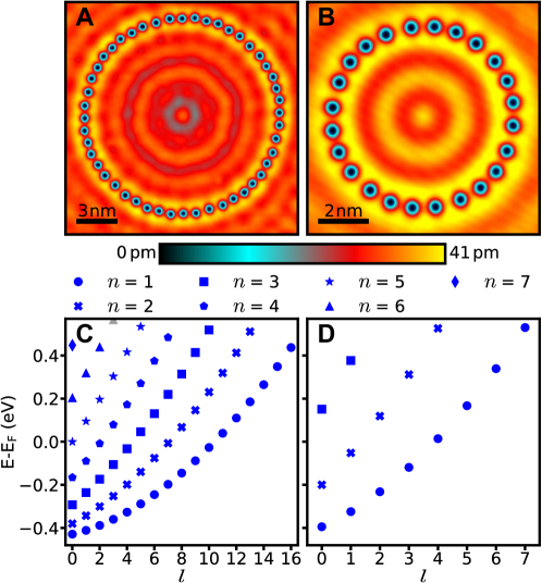
Figure 1: A: Constant current STM image ($10\,$mV/$10\,$pA) of a 48-CO quantum corral. B: STM image ($50\,$mV/$100\,$pA) of a 24-CO quantum corral. C & D: Calculated trapped states of the 48-CO corral and 24-CO corral, defined by the main quantum number $n$ and the angular momentum quantum number $l$ resulting from the hard wall model.

The corrals can be reasonably well described by an infinitely high, cylindrical potential well [8, 16], commonly known as the hard wall model. Solving the Schrödinger equation for this problem yields the solutions $\Psi_{n,l}(r,\phi,z)=\psi_{n,l}(r)\cdot\psi_{l}(\phi)\cdot\psi(z)$, where $n$ is the main quantum number and $l$ the angular momentum quantum number. The radial distance from the center of the corral is denoted with $r$, $\phi$ is the azimuthal angle and $z$ is the direction perpendicular to the surface. Here $\psi_{n,l}(r)$ describes the radial dependent component of the wavefunction including Bessel functions of the first kind and $\psi_{l}(\phi)=1/\sqrt{2\pi}\cdot\mathrm{exp}(il\phi)$ describes the angular dependence. The $z$-component of the Shockley surface state remains unaffected by the cylindrical potential well and above the surface, for $z>0$, $\psi(z)\propto\mathrm{exp}(-\kappa z)$ with the decay constant $\kappa$ [16]. The absolute square of each wavefunction, which can be measured with STM, gives the probability density $|\Psi_{n,l}(r,\phi,z)|^{2}=|\psi_{n,l}(r)|^{2}\cdot|\psi_{l}(\phi)|^{2}\cdot|\psi(z)|^{2}=|\psi_{n,l}(r)|^{2}\cdot 1/2\pi\cdot C_{z}$. Since for both corrals the respective measurements were performed with the same tip-sample distances and $\kappa$ is the same for every corral state [16] the z-component $|\psi(z)|^{2}$ simplifies to a constant factor $C_{z}$. For a more detailed discussion and calculations see the supplemental material of Stilp et al. [16]. In FIG. S2C & D the calculated energy spectra of the two corrals are displayed.

In order to study the corral, we performed scanning tunneling spectroscopy. However, performing stationary d$I$/d$V$ measurements (fixing $\vec{r}_{\mathrm{tip}}$ and sweeping the bias voltage $V_{\mathrm{B}}$) restricts analysis to the $l=0$ states. The reason for this is that one cannot find a suitable position $\vec{r}_{\mathrm{tip}}$ where a particular $l\neq 0$ state is energetically and spatially isolated. An example of this problem is shown in FIG. S2 of the supplemental material [17].

A complete description of the trapped electron states includes their energetic and spatial characteristics. By using d$I$/d$V$ line scans across the whole diameter of the corral (constant height measurements at a fixed sample bias) one can record the spatial behavior of the local density of states (LDOS) at a single energy $eV_{\mathrm{B}}$. We performed line scans over a bias range from $-450\,$mV to $400\,$mV across both corrals with increments of $5\,$mV. Combining these d$I$/d$V$ measurements results in FIG. 2 which represents a spatially (horizontal axis) and energetically (vertical axis) dependent local density of states (color coding) map of the quantum corral.

Each d$I$/d$V$ line scan (each horizontal line in FIG. 2) consists of a combination of several different states that, due to an energetic overlap, contribute at different magnitudes to the local density of states. By comparing the measured LDOS at different bias voltages with the absolute squares of the wave functions $|\psi_{n,l}(r)|^{2}$ obtained by the hard wall model one is able to reconstruct the energetic behavior of the states under study from the spatially resolved measurements.

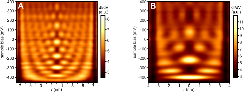
Figure 2: Differential conductance (d$I$/d$V$) as a function of radial distance $r$ from the center and sample bias of the (A) 48-CO corral and (B) 24-CO corral consisting of stacked d$I$/d$V$ line scans across the corrals. In A and B respectively the two outermost vertical, black stripes are originating from the CO molecules (corral walls). The bright appearing features can be assigned to the corral states. A Gaussian filter was used to flatten images A and B.

As Stilp [16] showed, atomic force microscopy images of a corral are proportional to the linear combination of all occupied corral states (states below the Fermi energy $E_{\mathrm{F}}$). From this study as well as from Crommie [8] it can be concluded that at each energy the measured d$I$/d$V$ signal is also a linear combination of states. The comparison between measurement and model was done by fitting every d$I$/d$V$ line scan with the following equation:

$$\frac{\mathrm{d}I}{\mathrm{d}V}(r,eV_{\mathrm{B}})\propto\sum\limits_{n,l}\alpha_{n,l}(eV_{\mathrm{B}})\cdot|\psi_{n,l}(r)|^{2}.$$ (1)

The prefactor $\alpha_{n,l}(eV_{\mathrm{B}})$ describes how much the probability density $|\psi_{n,l}(r)|^{2}$ contributes to the measured LDOS at a specific energy $eV_{\mathrm{B}}$. As an example a line scan obtained with $-170\,$mV across the $7.13\;$nm corral and the corresponding fit from equation (1) is shown in FIG. 3A. The excellent agreement between measurement and equation (1) supports the validity of the hard wall model.

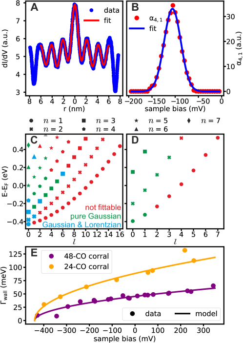
Figure 3: A Blue: Measured d$I$/d$V$ line scan at a sample bias of $V_{\mathrm{B}}=-170\,$meV across the 48-CO corral. Red: Fit of equation (1) to the measured curve. B: Red dots: Reconstructed energy distribution $\alpha_{4,1}$. Blue: Line shape analysis by fitting equation (2) to the energy distribution. C & D: Energy spectra of the 48-CO corral and 24-CO corral. Red markers: Due to an insufficient quality of the energy distribution a detailed line shape analysis was not possible. Green markers: Energy distributions with a pure Gaussian line shape. Cyan markers: Energy distributions with a Gaussian and a Lorentzian component. The mathematical description of the determination of the quality of an energy distribution is given in the supplemental material (SP3) [17]. E: Plot of $\Gamma_{\mathrm{wall}}$ after removing the known (Gaussian shaped) FWHM $\Gamma_{\mathrm{Fermi,RF}}$ from the general Gaussian shaped $\Gamma_{\mathrm{G,gen.}}$. Purple markers: $\Gamma_{\mathrm{wall}}$ for the 48-CO corral. Orange markers: $\Gamma_{\mathrm{wall}}$ for the 24-CO corral. Full lines: Plot of equation (4) with $x_{48}=9.26\,$nm and $x_{24}=4.75\,$nm.

By performing the fitting procedure for different bias voltages, we were able to determine the energetic dependence of several corral states, including $l\neq 0$ states. As an example, the energy distribution $\alpha_{4,1}$ is shown in FIG. 3B. All distributions reconstructed with the fitting method are given in the supplemental material (SP4) [17].

In order to characterize the energetic behavior of the trapped electron states we analyzed the energy distributions $\alpha_{n,l}$ in more detail. During d$I$/d$V$ measurements there will always be three broadening mechanisms which distort the original shape of spectral features. First there is the temperature dependent widening of the Fermi-Dirac distribution [18], which we will call Fermi-broadening. A second source of spectral broadening is radio-frequency-broadening (RF-broadening) [19, 20, 21, 22]. Both of these mechanisms cause a Gaussian shaped smearing of spectral features. Mathematically the combined broadening can be described as a convolution of two Gaussian broadening terms: $G_{\mathrm{Fermi,RF}}=G_{\mathrm{Fermi}}*G_{\mathrm{RF}}$. For the RF-broadening we estimate a FWHM of $\Gamma_{\mathrm{RF}}\approx 9\,$meV [19, 23] and for the Fermi-broadening at $\approx 5.7\,$K we calculate $\Gamma_{\mathrm{Fermi}}\approx 2\,$meV [18]. In total these two mechanism cause a Gaussian shaped smearing of spectroscopic features of $\Gamma_{\mathrm{Fermi,RF}}\approx 9.2\,$meV. The third mechanism of spectral broadening is modulation broadening which causes a smearing with the shape of a semicircle $\chi$ with a diameter of $2eV_{\mathrm{mod}}$ [18, 24].

The spectral feature itself is determined by intrinsic properties of the trapped Shockley surface state and the confinement. Multiple studies on noble metals revealed that there are multiple mechanisms which influence the lifetime of surface state electrons. These processes are electron-phonon scattering, electron-electron scattering and electron-defect scattering [25, 26, 27, 28, 29, 30]. The common property of the first two mechanisms is a temporally constant and spatially homogeneous scattering background for surface state electrons which can be expressed with an exponentially decreasing survival probability [30]. This exponential decay in the time domain results in a Lorentzian peak $L$ in the energy domain whereby the width of this peak is given by the decay constant of the exponential decrease. Furthermore, it is known that phononic and electronic decay channels are less efficient around the Fermi level [26, 27, 28, 31, 32] which results in a narrow width of these Lorentzian peaks in this energy region. Due to the spatial homogeneity of the electronic and phononic decay mechanisms, the width of the Lorentzian peaks stays unaffected by the size of the quantum structure. Electron-defect scattering on randomly distributed adsorbates would also result in a Lorentzian shaped peak component [30]. The electrons trapped in the quantum corral, however, do not interact with randomly distributed adsorbates. The structured arrangement of CO molecules leads to a spatially inhomogeneous scattering of surface state electrons. In contrast to electron-electron and electron-phonon scattering the spatially non-homogeneous electron-defect interaction should be sensitive to the size of the corral [33, 15]. This lifetime-limiting effect appears as a Gaussian peak $G_{\mathrm{wall}}$. Similar to the broadening mechanisms a trapped electron spectral feature is given by a convolution of the spatially homogeneous component and the spatially inhomogeneous part: $L*G_{\mathrm{wall}}$.

By combining $L*G_{\mathrm{wall}}$ with the broadening mechanisms $G_{\mathrm{Fermi,RF}}$ and $\chi$ a measured spectroscopic feature is described by the following equation:

$$\alpha_{n,l}\propto L*G_{\mathrm{wall}}*G_{\mathrm{Fermi,RF}}*\chi.$$ (2)

Fitting equation (2) to the energy distributions $\alpha_{n,l}$ gives an exact description of the line shape including the semicircular broadening $\chi$ with a modulation amplitude of $V_{\mathrm{mod}}=5\,$mV. For fitting, all Gaussian components of equation (2) were combined to a general Gaussian curve ($G_{\mathrm{G,gen.}}=G_{\mathrm{wall}}*G_{\mathrm{Fermi,RF}}$). The resulting fit of equation (2) to the energy distribution $\alpha_{4,1}$ is displayed in FIG. 3B and the following FWHM (full width at half maximum) for the Lorentzian and Gaussian component were obtained: $\Gamma_{\mathrm{L}}=0\,$meV & $\Gamma_{\mathrm{G,gen.}}=(42\pm 1)\,$meV. These fitting parameters directly show that the energy distribution $\alpha_{4,1}$ is purely described by a Gaussian peak shape. A prominent Gaussian behavior can further be found for most of the fittable energy distributions of the $7.13\;$nm and $3.57\;$nm corral. Interestingly some of the curves also have a small Lorentzian component. The presence of this measurable Lorentzian component is presented in FIG. 3C & D. However, even for these partly Lorentzian shaped curves the Gaussian component is bigger than the $9.2\,$meV that one would expect from only Fermi- and RF-broadening [34]. All reconstructed energy distributions and the complementary fits with equation (2) are shown in SP4 [17].

Investigating this dominant Gaussian broadening further, we removed the known widths of the Fermi- and the RF-broadening ($\Gamma_{\mathrm{Fermi,RF}}$) from the fitted FWHM of $G_{\mathrm{G,gen.}}$ to isolate $\Gamma_{\mathrm{wall}}$ [35]. Figure 3E is a plot of $\Gamma_{\mathrm{wall}}$ with respect to the distributions center energy [36]. From this graph it is clearly visible that the Gaussian shaped broadening mechanism shows a strong energy dependence. Furthermore $\Gamma_{\mathrm{wall}}$ monotonically increases with no minimum in the vicinity of $E_{F}$ which confirms that this component does not come from spatially homogeneous electronic and phononic decay. Another remarkable property of $\Gamma_{\mathrm{wall}}$ is that it depends on the size of the corral, meaning $G_{\mathrm{wall}}$ is sensitive to the size of the quantum structure.

To understand $G_{\mathrm{wall}}$ we propose a simple model which mathematically connects the energy dependency of $\Gamma_{\mathrm{wall}}$ with the size of the corral. As discussed above, our hypothesis is that $\Gamma_{\mathrm{wall}}$ is related to the interaction of the surface state electrons with the corral walls, e.g. by tunneling through the potential barrier given by the CO-molecules or inelastic scattering with the COs. In this context we first determine the path length $x$ an electron with a velocity of $v_{\mathrm{e}}$ can travel during its lifetime $T_{\mathrm{life}}$:

$$v_{\mathrm{e}}\cdot T_{\mathrm{life}}=\sqrt{\frac{2E}{m_{\mathrm{e}}^{*}}}\cdot T_{\mathrm{life}}=x.$$ (3)

Here $m_{\mathrm{e}}^{*}$ is given by the effective mass of surface state electrons on a Cu(111) surface which is $0.38$ times the mass of a free electron [37, 38]. Inserting $T_{\mathrm{life}}\approx\hbar/\Gamma$ in equation (3) then relates the spectral width $\Gamma$ with the path length $x$ of surface state electrons:

$$\Gamma=\frac{\hbar\sqrt{\frac{2E}{m_{e}^{*}}}}{x}.$$ (4)

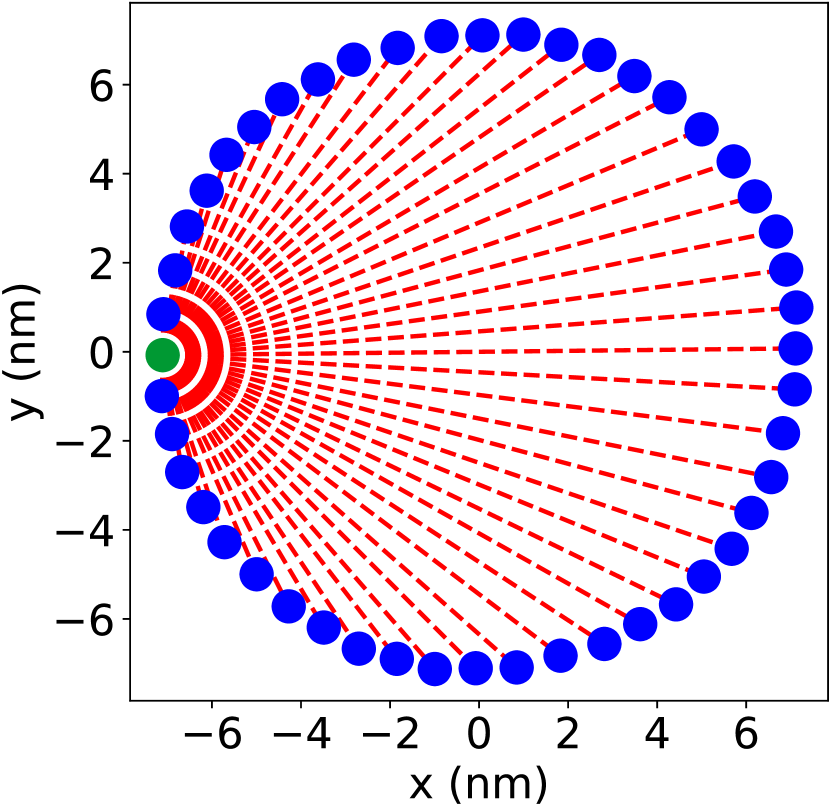
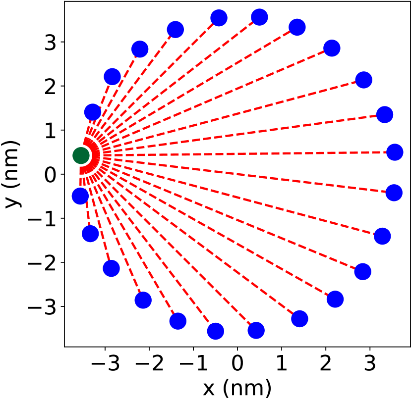
Figure S11: The average distance between a single CO (marked in green) and the remaining molecules (blue) in the corral wall gives a value of $9.26\,$nm for the big (left image) and $4.75\,$nm for the small corral (right image).

The values for $x$ follow from the calculation of the average distance between a single CO and the remaining molecules in the corral wall. For the $7.13\,$nm corral the average path length is $x_{48}=9.26\,$nm and for the $3.57\,$nm corral $x_{24}=4.75\,$nm (see illustration FIG. S11 [17]). The spectral widths derived from (4) with $x_{48}$ and $x_{24}$ respectively can be found in FIG. 3E. The excellent agreement between equation (4) and the measured data in FIG. 3E supports our hypothesis that the broadening $G_{\mathrm{wall}}$, which is the most dominant source of energy broadening, is caused by the confinement of the surface state or the interaction of the surface state electrons with the corral walls. Furthermore, equation (4) indicates that surface state electrons in both corrals have an energy independent average path length of $x_{48}=9.26\,$nm and $x_{24}=4.75\,$nm, receptively.

In summary we built two circular quantum corrals on a Cu(111) surface by positioning individual carbon monoxide molecules. By comparing the measured local density of states with a linear combination of the absolute squares of the wave functions obtained by the established hard wall model we reliably determined the energy distributions of $l\neq 0$ states. Analyzing these distributions revealed a dominant Gaussian shaped broadening of the states. Comparing the Gaussian broadening components for the two corrals yielded a clear correlation between the size of the quantum structure and the spectral width. A model relating the spectral width of resonant eigenstates with the single particle movement of surface state electrons reveals that the Gaussian broadening mechanism is caused by the interaction between the surface state electrons and the corral wall. A model description for the explicit shape of the Gaussian broadening term could be subject of future theoretical investigation.

Supplemental Material

SP1 Experimental setup

Microscope The experiments were performed on a home-built combined atomic force and scanning tunneling microscope with a base temperature of $\approx 5.7\,$K. The system operates with a qPlus sensor [1] which was equipped with an electrochemically etched tungsten tip. The bias voltage is applied to the sample. The Cu(111) sample was prepared with standard sputter and anneal cycles.

Measurement settings The d$I$/d$V$ line scans across the corral diameter have a length of $18\,$nm for the 48-CO corral and a length of $10\,$nm for the 24-CO corral. Every line scan was performed in constant height. Each scan consists of an average over 7 line scans acquired with a scan speed of $2\,$nm/s and 1024 pixels per line. For the 48-CO corral a setpoint of $-170\,$mV/$170\,$pA and for the 24-CO corral a setpoint of $100\,$mV/$100\,$pA was used with the tip positioned at the center of each corral. For the acquisition of the differential conductance we modulated the sample bias by a sinusoidal AC voltage with an amplitude of $V_{\mathrm{mod}}=5\,$mV and a frequency of $600\,$Hz. For the modulation frequency we chose a low noise region in the power spectral density spectrum of the tunneling current (see Figure S1).

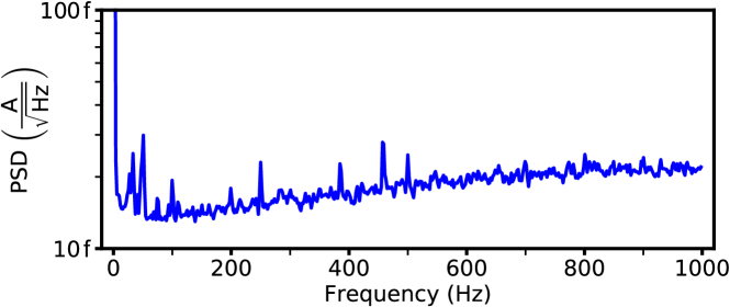
Figure S1: Power spectral density (PSD) as a function of frequency in constant height over the center of the 48-CO corral at a sample bias of $-10\,$mV and a tunneling current of $10\,$pA.

SP2 Stationary dI/dV measurements in the 48 CO corral

As an example two stationary d$I$/d$V$ spectra are displayed in Fig S2. The red curve is a measurement over the center of the $7.13\,$nm corral and is therefore only sensitive to the $l=0$ states. The second curve (green) was measured $900\,$pm off center. A d$I$/d$V$ spectrum at this position is sensitive to $l=0$ and $l=1$ states which results in additional spectral peaks. Because of an overlay of several peaks one can only see the top most part of the states energy distributions. Since a Gaussian and Lorentz distribution are very similar near their maxima, a proper line shape analysis is not possible. Therefore d$I$/d$V$ at single points above the corral for a detailed line shape study of $l\neq 0$ states is not reliable.

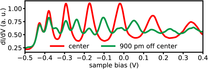
Figure S2: Two d$I$/d$V$ spectra measured inside the 48-CO corral at different positions. Red: center of the corral; Green: $900\,$mV off center.

SP3 Quality of the reconstructed energy distribution

To quantify the quality of the reconstructed energy distributions $\alpha_{n,l}$ we used the relative quadratic deviation between every distribution and the fit with equation (2) of the main text.

$$\mathrm{RQD}=\dfrac{{\sum\limits_{i=0}^{n}}\biggl{[}\alpha_{n,l}\Bigl{(}V_{B}^{(i)}\Bigr{)}-\mathrm{F}\Bigl{(}V_{B}^{(i)}\Bigr{)}\biggr{]}^{2}}{{\sum\limits_{i=0}^{n}}\biggl{[}\mathrm{F}\Bigl{(}V_{B}^{(i)}\Bigr{)}\biggl{]}^{2}}$$ (1)

In this formula $\alpha_{n,l}\Bigl{(}V_{B}^{(i)}\Bigr{)}$ describes the value of the energy distribution at the sample voltage $V_{B}^{(i)}$ and $\mathrm{F}\Bigl{(}V_{B}^{(i)}\Bigr{)}$ is given by the value of the fit of equation (2) in the main text at the same bias voltage. As a final step the quality $\xi$ of the energy distribution can be defined as

$$\xi=1-\mathrm{RQD}$$ (2)

In order to maximize the over all accuracy of the line shape analysis presented in the main text only distributions with a $\xi$-value between $1$ and $0.85$ were analyzed further. Distributions with $\xi\geq 0.85$ are depicted in FIG. 3C (main text) with green and cyan colors whereas low quality energy distributions ($\xi<0.85$) are marked in red.

SP4 Energy distributions and fits for the big and small corral

The fits of the distributions were done with equation (2) of the main text. Afterwards the quality value $\xi$ was determined as described in SP3. In this section all the reconstructed energy distributions with $\xi\geq 0.85$ are presented.

SP4.1 $l=0$ states - big corral

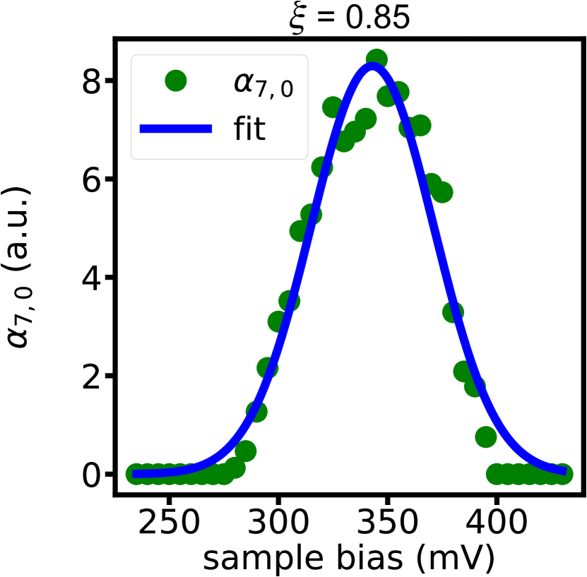
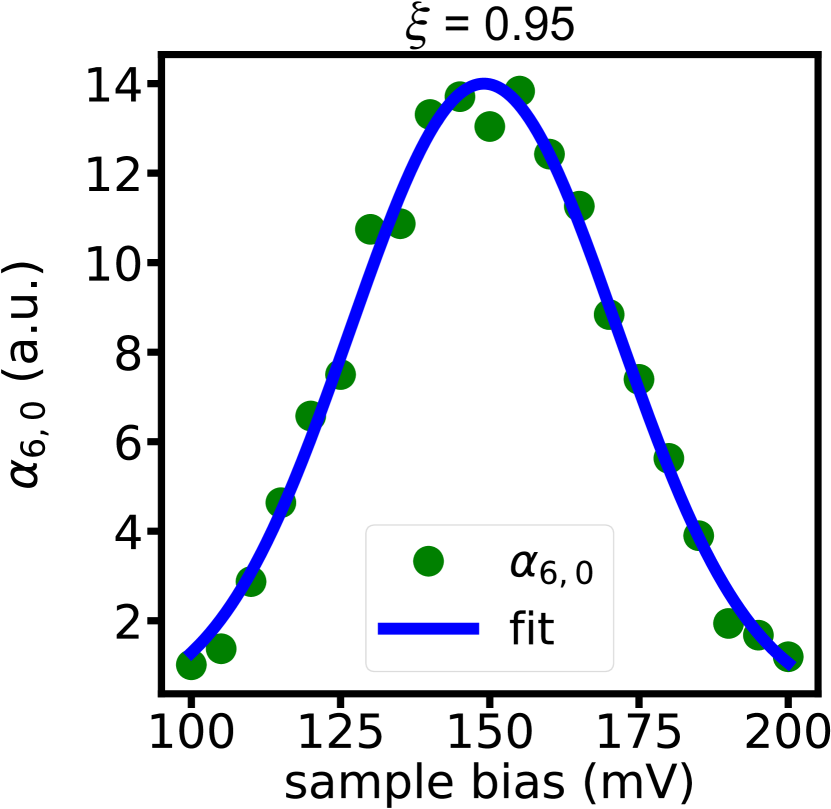
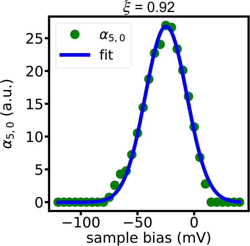
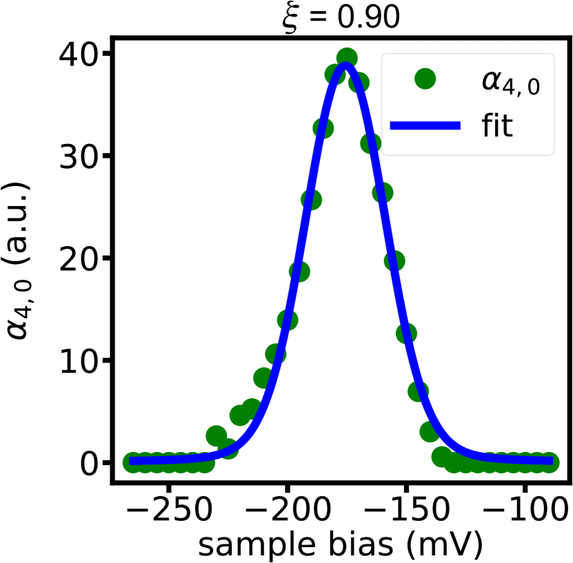
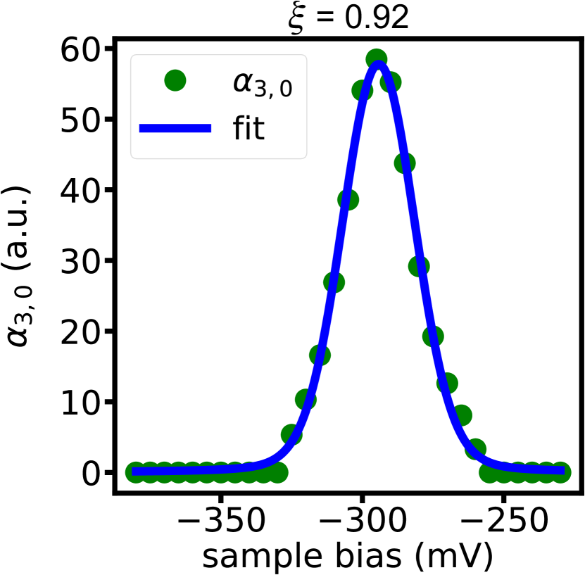
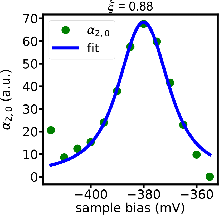
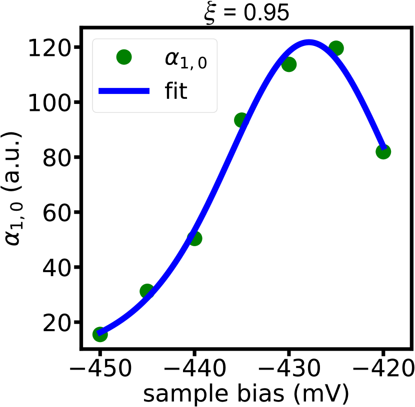
Figure S3: Reconstructed energy distributions for the $l=0$ states (green dots). For the detailed line shape analysis equation (2) (main text) was fitted to the distributions. The fit is depicted with a full, blue line. The quality value $\xi$ can be found above each plot and was calculated as described in SP3.

$n=7,l=0$	fit (meV)
$\Gamma_{\mathrm{G,gen.}}$	$66\pm 7$
$\Gamma_{\mathrm{L}}$	0
$E_{\mathrm{7,0}}$	$-$$343.0\pm 0.9$

$n=6,l=0$	fit (meV)
$\Gamma_{\mathrm{G,gen.}}$	$52\pm 7$
$\Gamma_{\mathrm{L}}$	0
$E_{\mathrm{6,0}}$	$-$$149.0\pm 0.4$

$n=5,l=0$	fit (meV)
$\Gamma_{\mathrm{G,gen.}}$	$43\pm 3$
$\Gamma_{\mathrm{L}}$	0
$E_{\mathrm{5,0}}$	$0$$-24.7\pm 0.4$

$n=4,l=0$	fit (meV)
$\Gamma_{\mathrm{G,gen.}}$	$37\pm 3$
$\Gamma_{\mathrm{L}}$	$4\pm 3$
$E_{\mathrm{4,0}}$	$-175.6\pm 0.4$

$n=3,l=0$	fit (meV)
$\Gamma_{\mathrm{G,gen.}}$	$28\pm 2$
$\Gamma_{\mathrm{L}}$	$4\pm 2$
$E_{\mathrm{3,0}}$	$-294.3\pm 0.2$

$n=2,l=0$	fit (meV)
$\Gamma_{\mathrm{G,gen.}}$	$8\pm 13$
$\Gamma_{\mathrm{L}}$	$18\pm 7$
$E_{\mathrm{2,0}}$	$-380.0\pm 0.8$

$n=1,l=0$	fit (meV)
$\Gamma_{\mathrm{G,gen.}}$	$13\pm 6$
$\Gamma_{\mathrm{L}}$	$12\pm 6$
$E_{\mathrm{1,0}}$	$-427.9\pm 0.4$

Table 3: Results for fitting equation (2) of the main text to the reconstructed $l=0$ energy distributions of the big corral.

SP4.2 $l=1$ states - big corral

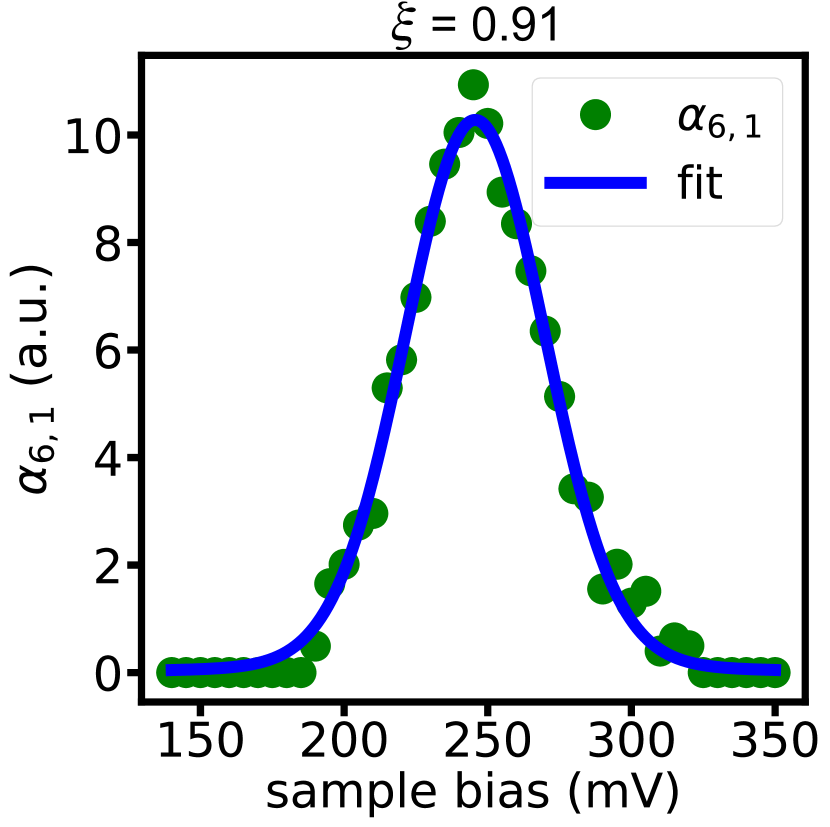
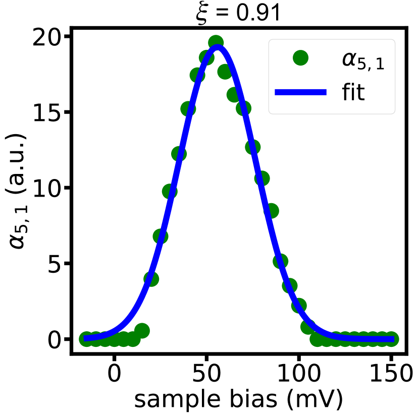
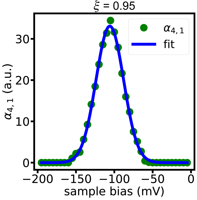
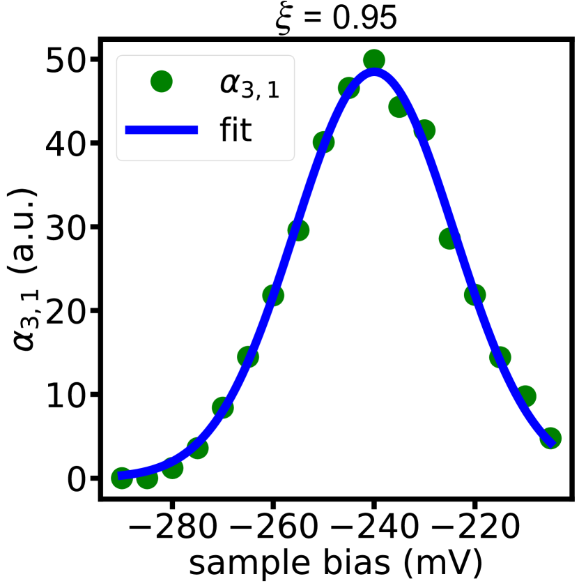
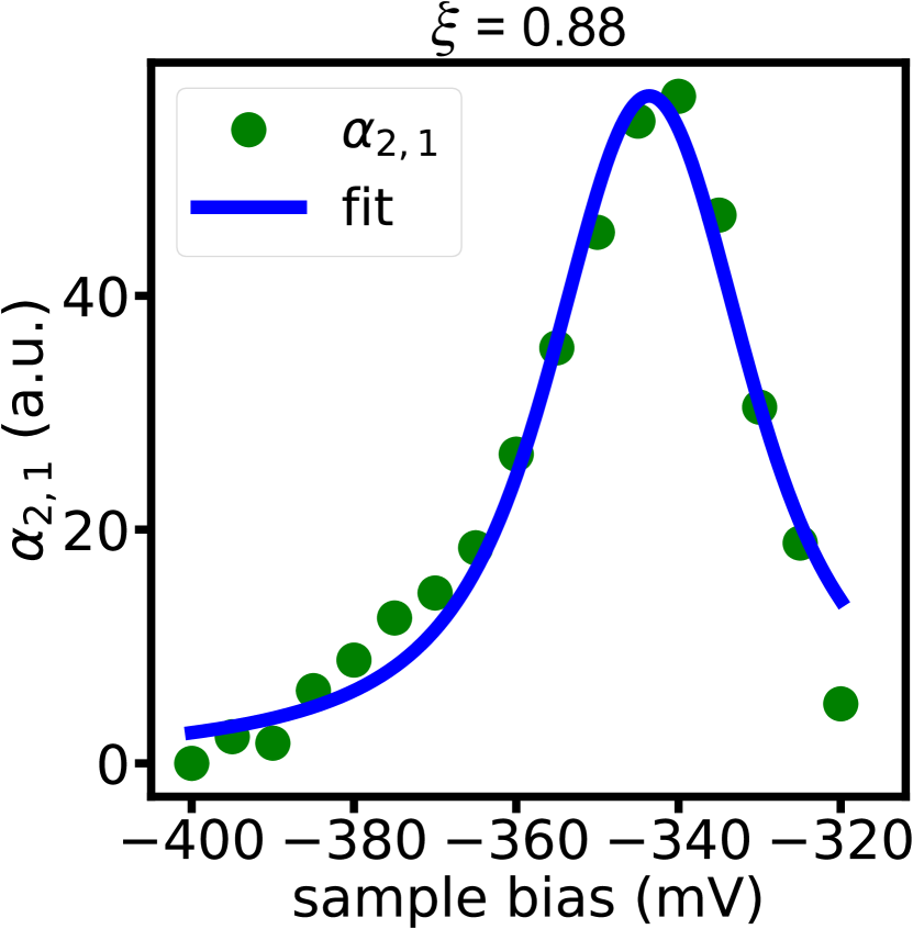
Figure S4: Reconstructed energy distributions for the $l=1$ states (green dots). For the detailed line shape analysis equation (2) (main text) was fitted to the distributions. The fit is depicted with a full, blue line. The quality value $\xi$ can be found above each plot and was calculated as described in SP3.

$n=6,l=1$	fit (meV)
$\Gamma_{\mathrm{G,gen.}}$	$55\pm 3$
$\Gamma_{\mathrm{L}}$	$4\pm 4$
$E_{\mathrm{6,1}}$	$-$$245.6\pm 0.4$

$n=5,l=1$	fit (meV)
$\Gamma_{\mathrm{G,gen.}}$	$49\pm 4$
$\Gamma_{\mathrm{L}}$	0
$E_{\mathrm{5,1}}$	$-$$55.8\pm 0.5$

$n=4,l=1$	fit (meV)
$\Gamma_{\mathrm{G,gen.}}$	$42\pm 1$
$\Gamma_{\mathrm{L}}$	0
$E_{\mathrm{4,1}}$	$-105.9\pm 0.2$

$n=3,l=1$	fit (meV)
$\Gamma_{\mathrm{G,gen.}}$	$37\pm 3$
$\Gamma_{\mathrm{L}}$	$0$
$E_{\mathrm{3,1}}$	$-240.0\pm 0.3$

$n=2,l=1$	fit (meV)
$\Gamma_{\mathrm{G,gen.}}$	$12\pm 9$
$\Gamma_{\mathrm{L}}$	$22\pm 6$
$E_{\mathrm{2,1}}$	$-343.6\pm 0.6$

Table 4: Results for fitting equation (2) of the main text to the reconstructed $l=1$ energy distributions of the big corral.

SP4.3 $l=2$ states - big corral

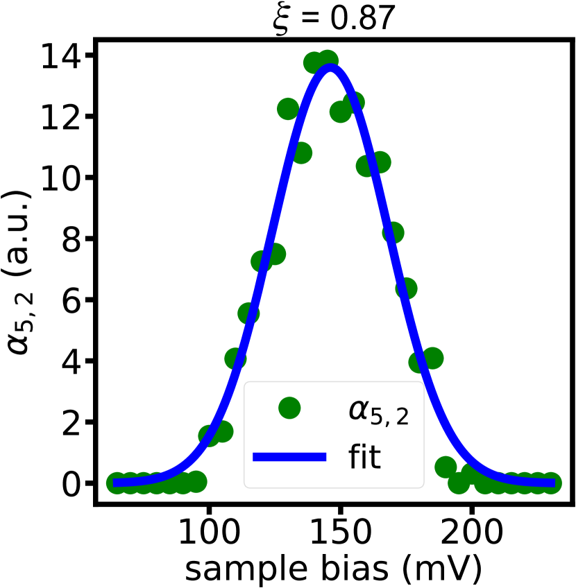
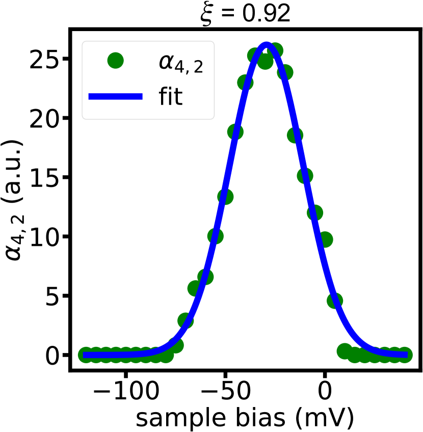
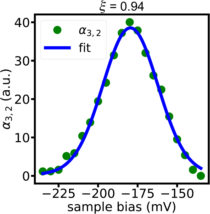
Figure S5: Reconstructed energy distributions for the $l=2$ states (green dots). For the detailed line shape analysis equation (2) (main text) was fitted to the distributions. The fit is depicted with a full, blue line. The quality value $\xi$ can be found above each plot and was calculated as described in SP3.

$n=5,l=2$	fit (meV)
$\Gamma_{\mathrm{G,gen.}}$	$52\pm 5$
$\Gamma_{\mathrm{L}}$	0
$E_{\mathrm{5,2}}$	$-$$146.1\pm 0.7$

$n=4,l=2$	fit (meV)
$\Gamma_{\mathrm{G,gen.}}$	$44\pm 3$
$\Gamma_{\mathrm{L}}$	0
$E_{\mathrm{4,1}}$	$-29.4\pm 0.4$

$n=3,l=2$	fit (meV)
$\Gamma_{\mathrm{G,gen.}}$	$39\pm 4$
$\Gamma_{\mathrm{L}}$	$3\pm 5$
$E_{\mathrm{3,2}}$	$-179.6\pm 0.4$

Table 5: Results for fitting equation (2) of the main text to the reconstructed $l=2$ energy distributions of the big corral.

SP4.4 $l=3$ states - big corral

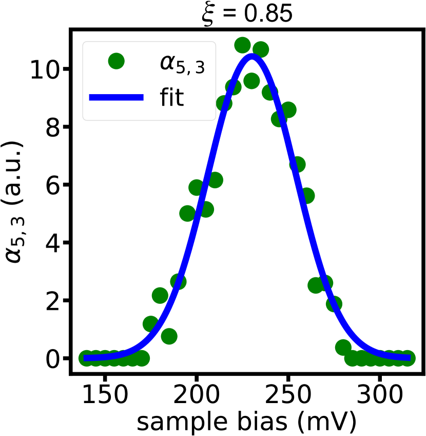
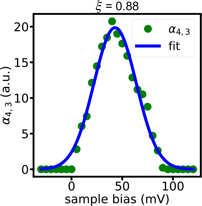
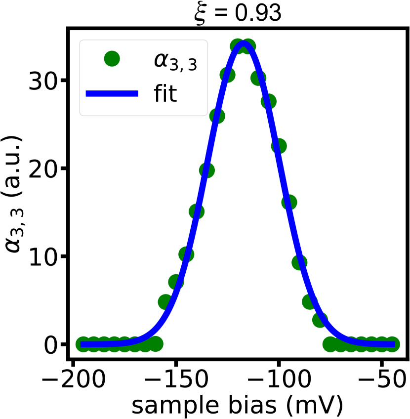
Figure S6: Reconstructed energy distributions for the $l=3$ states (green dots). For the detailed line shape analysis equation (2) (main text) was fitted to the distributions. The fit is depicted with a full, blue line. The quality value $\xi$ can be found above each plot and was calculated as described in SP3.

$n=5,l=3$	fit (meV)
$\Gamma_{\mathrm{G,gen.}}$	$57\pm 6$
$\Gamma_{\mathrm{L}}$	0
$E_{\mathrm{5,3}}$	$-$$230.2\pm 0.8$

$n=4,l=3$	fit (meV)
$\Gamma_{\mathrm{G,gen.}}$	$49\pm 5$
$\Gamma_{\mathrm{L}}$	0
$E_{\mathrm{4,3}}$	$43.0\pm 0.6$

$n=3,l=3$	fit (meV)
$\Gamma_{\mathrm{G,gen.}}$	$41\pm 2$
$\Gamma_{\mathrm{L}}$	$0$
$E_{\mathrm{3,3}}$	$-117.3\pm 0.3$

Table 6: Results for fitting equation (2) of the main text to the reconstructed $l=3$ energy distributions of the big corral.

SP4.5 $l=4$, $l=5$ and $l=6$ states - big corral

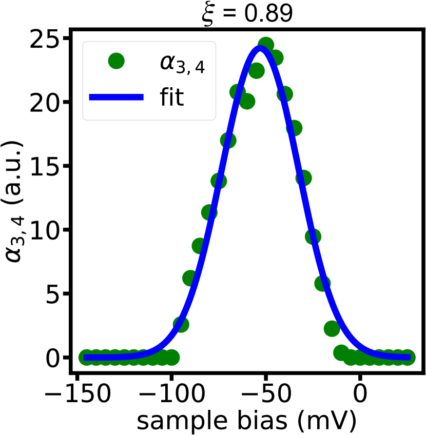
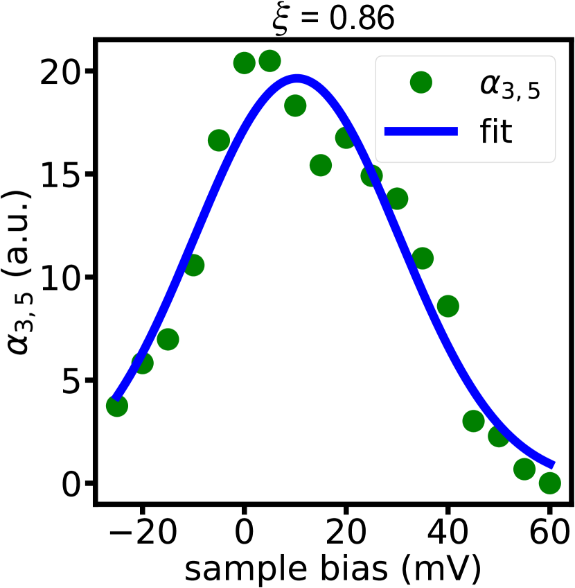
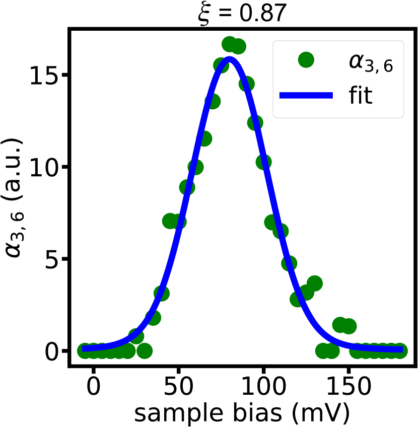
Figure S7: Reconstructed energy distributions for the $l=4$, $l=5$ and $l=6$ states (green dots). For the detailed line shape analysis equation (2) (main text) was fitted to the distributions. The fit is depicted with a full, blue line. The quality value $\xi$ can be found above each plot and was calculated as described in SP3.

$n=3,l=4$	fit (meV)
$\Gamma_{\mathrm{G,gen.}}$	$48\pm 4$
$\Gamma_{\mathrm{L}}$	0
$E_{\mathrm{3,4}}$	$-53.0\pm 5$

$n=3,l=5$	fit (meV)
$\Gamma_{\mathrm{G,gen.}}$	$47\pm 16$
$\Gamma_{\mathrm{L}}$	0
$E_{\mathrm{3,5}}$	$10\pm 1$$0$

$n=3,l=6$	fit (meV)
$\Gamma_{\mathrm{G,gen.}}$	$50\pm 5$
$\Gamma_{\mathrm{L}}$	$5\pm 7$
$E_{\mathrm{3,6}}$	$79.9\pm 0.7$

Table 7: Results for fitting equation (2) of the main text to the reconstructed $l=4$, $l=5$ and $l=6$ energy distributions of the big corral.

SP4.6 $l=0$ states - small corral

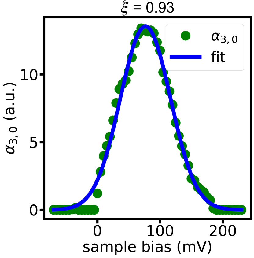
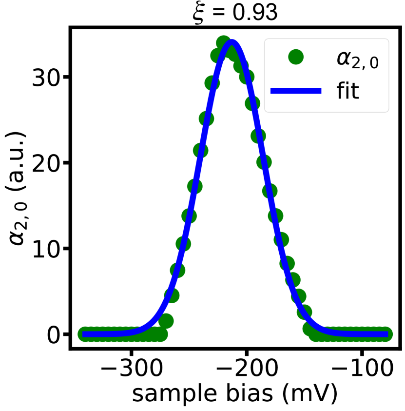
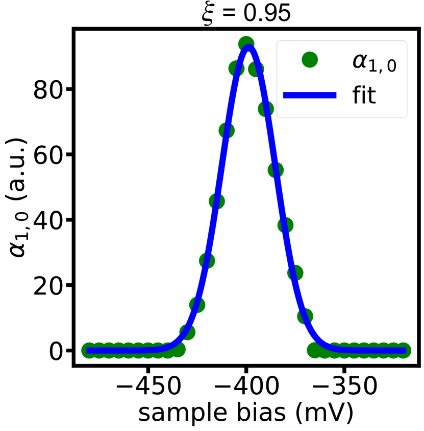
Figure S8: Reconstructed energy distributions for the $l=0$ states (green dots). For the detailed line shape analysis equation (2) (main text) was fitted to the distributions. The fit is depicted with a full, blue line. The quality value $\xi$ can be found above each plot and was calculated as described in SP3.

$n=3,l=0$	fit (meV)
$\Gamma_{\mathrm{G,gen.}}$	$94\pm 5$
$\Gamma_{\mathrm{L}}$	0
$E_{\mathrm{3,0}}$	$0$ $76.6\pm 0.6$ $0$

$n=2,l=0$	fit (meV)
$\Gamma_{\mathrm{G,gen.}}$	$64\pm 3$
$\Gamma_{\mathrm{L}}$	0
$E_{\mathrm{2,0}}$	$-213.0\pm 0.4$

$n=1,l=0$	fit (meV)
$\Gamma_{\mathrm{G,gen.}}$	$32\pm 1$
$\Gamma_{\mathrm{L}}$	$0$
$E_{\mathrm{1,0}}$	$-398.8\pm 0.2$

Table 8: Results for fitting equation (2) of the main text to the reconstructed $l=0$ energy distributions of the small corral.

SP4.7 $l=1$ states - small corral

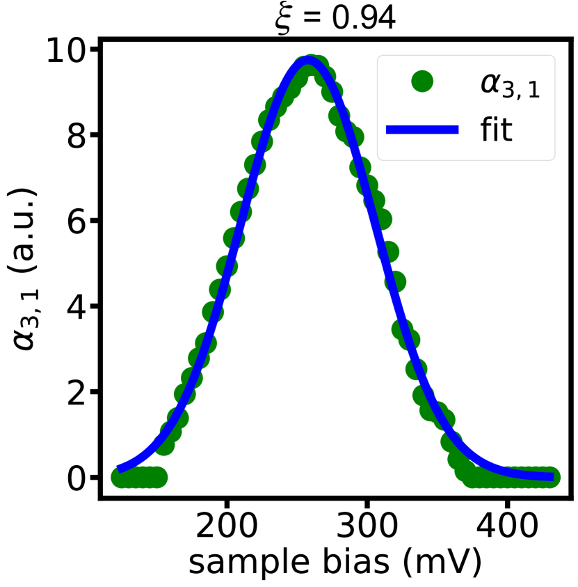
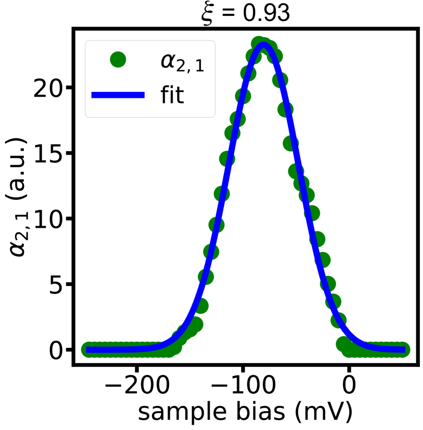
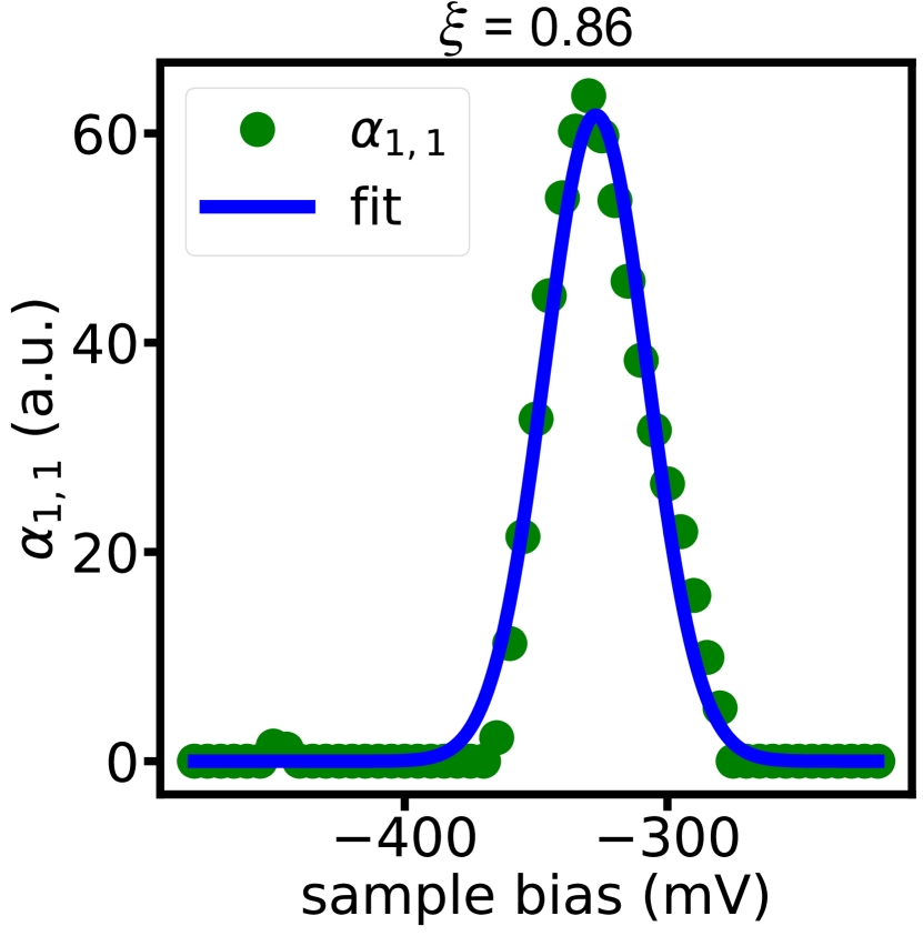
Figure S9: Reconstructed energy distributions for the $l=1$ states (green dots). For the detailed line shape analysis equation (2) (main text) was fitted to the distributions. The fit is depicted with a full, blue line. The quality value $\xi$ can be found above each plot and was calculated as described in SP3.

$n=3,l=1$	fit (meV)
$\Gamma_{\mathrm{G,gen.}}$	$113\pm 5$
$\Gamma_{\mathrm{L}}$	0
$E_{\mathrm{3,1}}$	$257.7\pm 0.5$

$n=2,l=1$	fit (meV)
$\Gamma_{\mathrm{G,gen.}}$	$77\pm 3$
$\Gamma_{\mathrm{L}}$	0
$E_{\mathrm{2,1}}$	$-80.6\pm 0.4$

$n=1,l=1$	fit (meV)
$\Gamma_{\mathrm{G,gen.}}$	$46\pm 3$
$\Gamma_{\mathrm{L}}$	$0$
$E_{\mathrm{1,1}}$	$-327.3\pm 0.5$

Table 9: Results for fitting equation (2) of the main text to the reconstructed $l=1$ energy distributions of the small corral.

SP4.8 $l=2$ and $l=3$ states - small corral

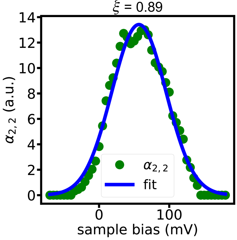
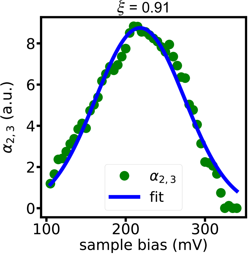
Figure S10: Reconstructed energy distributions for the $l=2$ and $l=3$ states (green dots). For the detailed line shape analysis equation (2) (main text) was fitted to the distributions. The fit is depicted with a full, blue line. The quality value $\xi$ can be found above each plot and was calculated as described in SP3.

$n=2,l=2$	fit (meV)
$\Gamma_{\mathrm{G,gen.}}$	$91\pm 7$
$\Gamma_{\mathrm{L}}$	0
$E_{\mathrm{2,2}}$	$56.8\pm 0.8$

$n=2,l=3$	fit (meV)
$\Gamma_{\mathrm{G,gen.}}$	$132\pm 23$
$\Gamma_{\mathrm{L}}$	0
$E_{\mathrm{2,3}}$	$218\pm 2$

Table 10: Results for fitting equation (2) of the main text to the reconstructed $l=2$ and $l=3$ energy distributions of the big corral.

SP5 Average distance between a single CO and the remaining molecules

References

- Verolainen and Nikolaich [1982] F. J. Giessibl, High-speed force sensor for force microscopy and profilometry utilizing a quartz tuning fork, Applied Physics Letters 73, 3956 (1998).