DNeRV: Modeling Inherent Dynamics via Difference Neural Representation for Videos

Abstract

Existing implicit neural representation (INR) methods do not fully exploit spatiotemporal redundancies in videos. Index-based INRs ignore the content-specific spatial features and hybrid INRs ignore the contextual dependency on adjacent frames, leading to poor modeling capability for scenes with large motion or dynamics. We analyze this limitation from the perspective of function fitting and reveal the importance of frame difference. To use explicit motion information, we propose Difference Neural Representation for Videos (DNeRV), which consists of two streams for content and frame difference. We also introduce a collaborative content unit for effective feature fusion. We test DNeRV for video compression, inpainting, and interpolation. DNeRV achieves competitive results against the state-of-the-art neural compression approaches and outperforms existing implicit methods on downstream inpainting and interpolation for $960\times 1920$ videos.

1 Introduction

In recent years, implicit neural representations (INR) have gained significant attention due to their strong ability in learning a coordinate-wise mapping of different functions. The main principle behind INR is to learn an implicit continuous mapping $f$ using a learnable neural network $g_{\theta}(\cdot):\mathbb{R}^{m}\rightarrow\mathbb{R}^{n}$. The idea was first proposed for the neural radiance fields (NeRF) [28] and since then has been applied to various applications [8, 58, 4].

INR attempts to approximate the continuous $f$ by training $g_{\theta}$ with $m$-dimensional discrete coordinates $\mathbf{x}\in\mathbb{R}^{m}$ and corresponding quantity of interest $\mathbf{y}\in\mathbb{R}^{n}$. Once trained, the desired $f$ can be fully characterized using $g_{\theta}$ or the weights $\theta$, and it would be benefit for the tasks which need to model the intrinsic generalization for given data, such as interpolation or inpainting tasks shown in Fig. 1.

The success of INR can be attributed to the insight that a learnable and powerful operator with a finite set of data samples $\mathcal{S}=\{{x_{i},y_{i}}\}^{N}_{i=0}$, can fit the unknown mapping $f$. The accuracy of the mapping depends on the number of samples $(N)$ and the complexity of the map $f$. INR for videos requires a large $N$, which primarily depends on the size and internal complexity of the video sequence. Furthermore, video representation is complicated due to different sampling or frames-per-second (FPS) rates of videos. Large motion (in terms of direction, speed, rotation, or blur) and transformations of the objects or scene can make adjacent frames quite different. Figure 2 shows examples of such mismatch between consecutive frames, which we attribute to adjacent dynamics.

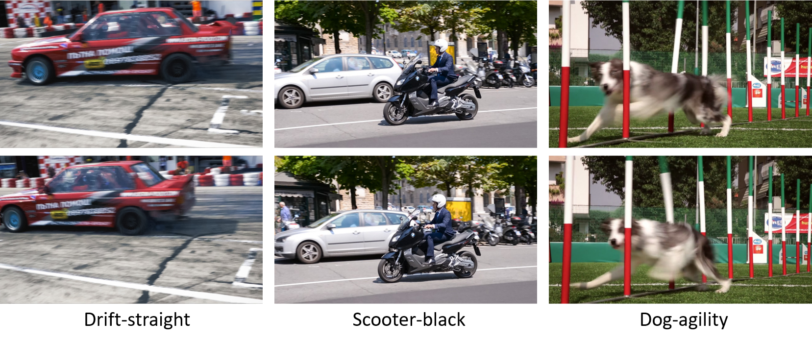
Figure 2: Examples of neighboring frames with large mismatch. Learning continuous INR with such dynamics is challenging.

Adjacent dynamics are the short-term transformations in the spatial structure, which are difficult to represent using existing methods for neural representation of videos (NeRV). Existing NeRV approaches can be broadly divided into two groups: (1) Index-based methods, such as [4] and [21], use positional embedding of the index as input and lack content-specific information for given videos. (2) Hybrid-based methods [1] use frames for index embedding and neglect the temporal correlation between different frames. Therefore, neither index nor frame-based NeRV are effective against adjacent dynamics.

In this work, we propose Difference NeRV (DNeRV) that attempts to approximate a dynamical system by absorbing the difference of adjacent frames, $\mathbf{y}^{D}_{t}=\mathbf{y}_{t}-\mathbf{y}_{t-1}$ and $\mathbf{y}^{D}_{t+1}=\mathbf{y}_{t+1}-\mathbf{y}_{t}$, as a diff stream input. Further analysis for the importance of diff stream is presented in Section 3. An illustration of DNeRV pipeline is presented in Figure 3. Diff encoder captures short-term contextual correlation in the diff stream, which is then merged with the content stream for spatiotemporal feature fusion. In addition, we propose a novel gated mechanism, collaborative content unit (CCU), which integrates spatial features in the content stream and temporal features in the diff stream to obtain accurate reconstruction for those frames with adjacent dynamics.

The main contribution of this paper are as follows.

• Existing NeRV methods cannot model content-specific features and contextual correlations simultaneously. We offer an explanation using adjacent dynamics. Furthermore, we reveal the importance of diff stream through heuristic analysis and experiments.

• We propose the Difference NeRV, which can model the content-specific spatial features with short-term temporal dependence more effectively and help network fit the implicit mapping efficiently. We also propose a collaborative content unit to merge the features from two streams adaptively.

• We present experiments on three datasets (Bunny, UVG, and Davis Dynamic) and various downstream tasks to demonstrate the effectiveness of the proposed method. The superior performance over all other implicit methods shows the efficacy of modeling videos with large motion. As a result, DNeRV can be regarded as a new baseline for INR-based video representation.

2 Related Work

Implicit neural representations (INRs) have been used in various vision tasks in recent years [6, 28]. In 3D vision, [27, 24, 31, 51, 51] aim to use INRs from static and simple to dynamic and complicated visual data. In image analysis, INRs have been used to learn the mapping between 2D spatial coordinates $\mathbf{x}\in\mathbb{R}^{2}$ and corresponding RGB value $\mathbf{y}\in\mathbb{R}^{3}$ via various positional embedding techniques [39, 43, 9, 55] or meta-learning [40]. In video analysis, INRs learn the mapping from frame index $x_{t}\in\mathbb{R}$ to RGB frame $\mathbf{y}\in\mathbb{R}^{3\times w\times h}$ [4, 5, 25]. In other visual tasks, INRs can encode both spatial coordinates and specific feature vectors [36, 53].

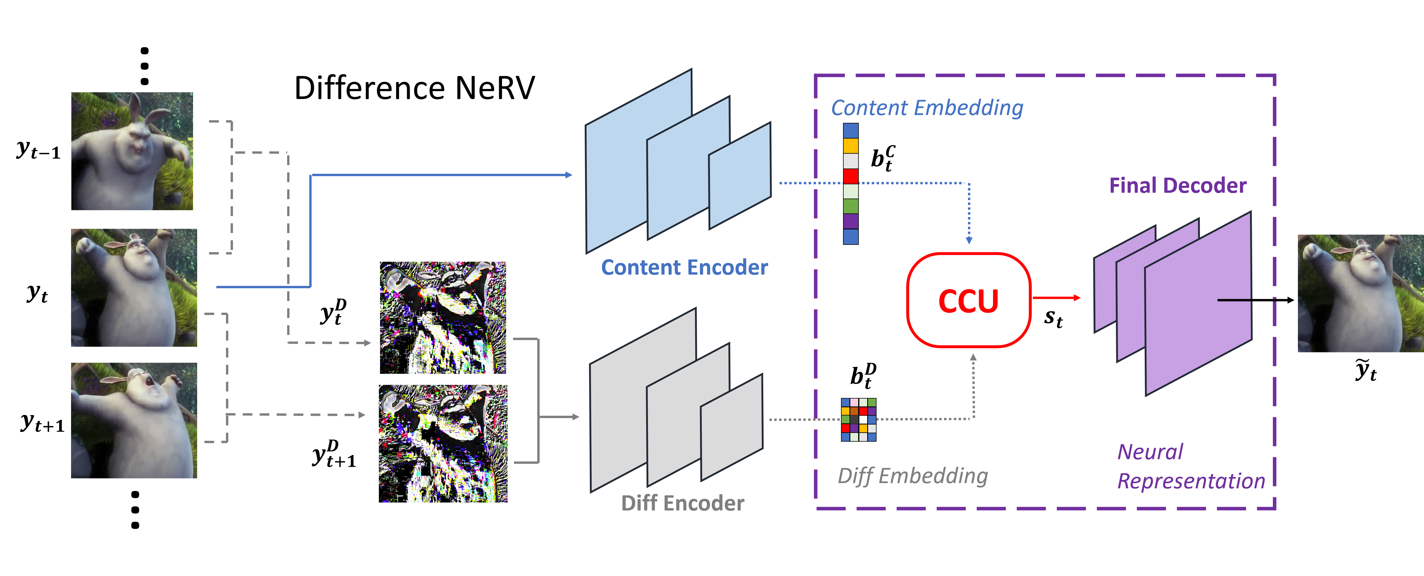
Figure 3: The pipeline of DNeRV. Blue part indicates content stream, grey for diff stream and red for fusion. The purple part is the implicit neural representation for the given video, consisting of embeddings, lightweight CCU, and decoder.

Neural representation for videos (NeRV) methods can be broadly divided into two groups. Index-based NeRV methods use the positional embedding of $t$ as the input [4, 21, 25]. The follow-up work has improved network structure for acceleration or disentangled feature modeling, but those methods could not capture the content-specific information, causing spatial redundancy. Hybrid-based NeRV [1] provides an insightful view by treating the current frame itself as the index embedding. The method shows much better performance over index-based ones via content-adaptive fashion. The main limitation of hybrid NeRV is that they ignore temporal relationship between frames, resulting in poor performance with adjacent dynamics.

Video compression methods based on INR use the traditional pipeline but change some intermediate components into networks [23, 15, 22, 19, 33]. However, their utility is limited by large number of parameters and computational redundancy, causing long coding time and limited generalized ability. One significance of INRs for video is that the video compression can be regarded as a model compression problem, and the existing model compression and acceleration techniques [12, 11] could be used for INR-based network. Neural compression is expected to break through the limitation of traditional pipeline with the help of INRs, resulting in better performance.

Two stream vision and fusion resemble the idea of adopting multi-stream mechanism for disentangling feature learning in video analysis. [35] observe the importance of optical flow, which is widely used in action recognition [38, 10, 3] or other visual tasks [42, 16]. Separating motion and content as two stream is also widely used in video prediction [44] and image-to-video generation [57]. Furthermore, hidden state and time-dependent input in RNN/LSTM could be thought as different stream [14, 7, 46]. More effective fusion module for different stream information is a fundamental task in sequence learning, generating lots of novel gated mechanism [45, 56, 13]. The two-stream fusion aims to reduce the spatiotemporal redundancy caused by the inherent continuity of video, which motivated us to propose DNeRV based on diff stream. Additionally, inspired by the gated mechanism in RNN, we introduce a fusion unit for adaptive feature fusion.

3 Motivation

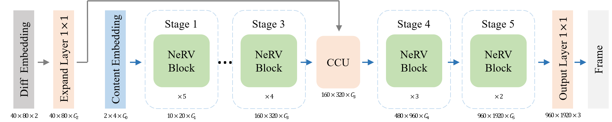
Figure 4: Architecture of decoder with CCU as fusion module for $960\times 1920$.

In this section, we discuss how the frame differences benefit the adjacent dynamics. A video sequence is a collection of images captured over time; therefore, motion of different objects in video is often spatially continuous and smooth. The main objective of INR is to learn an implicit mapping $f(\mathbf{x})\mapsto\mathbf{y}$. Thus, we usually assume that training tuples $(\mathbf{x},\mathbf{y})$ are dense enough so that the continuous $f$ can be approximated. In the case of NeRV, the difference between frames (or the so-called adjacent dynamics) violates the expected smoothness. That is the main reason for the failure of NeRV in the presence of large motion and highly dynamic scenes.

For video INRs, the training data are $\{(t,\mathbf{y}_{t})\}_{t=0}^{N}$, where $\mathbf{y}_{t}$ is the frame at time index $t$. We assume that the implicit (unknown) mapping $f$ is continuous and defined as

$$f:\Phi\rightarrow\mathbb{R}^{3\times H\times W},\quad\Phi=[0,N].$$ (1)

Let us note that although NeRV methods use various positional encoding techniques [43, 39] to map the discrete index into a higher dimension for better performance (we treat the frame itself as an embedding of the index for hybrid-based methods, the network $g_{\theta}$ is actually a mapping from a time index in $\Phi$ to $\mathbb{R}^{3\times H\times W}$. Once trained, we can generate frames as

$$g_{\theta}\left(t\right)=\mathbf{y}_{t},\quad t\in\{1,2,\cdots,N\}.$$ (2)

Since video is usually continuous along spatial and temporal dimensions, $f$ can also be described as a dynamical system:

$$\dot{f}=A(f(t),t),$$

where $A(\cdot,\cdot)$ represents a nonlinear function determined by the system. The goal of INR is to use the neural network $g_{\theta}$ to fit the $f$ with the training tuples $\{(t,f(t))\}_{t=0}^{N}$. However, in general, the training tuple $(t,f(t))$ is not enough for networks to learn a dynamical system. For example, we consider a simple time-invariant system:

$$\dot{f}=A\cdot f(t),\quad f(0)=\mathbf{y}_{0},$$

where $A$ is a constant. The solution of the problem can be written as $f(t)=\exp(At)\mathbf{y}_{0}$. If $g_{\theta}$ is a general feed-forward ReLU network, then we can achieve $\|g_{\theta}(t)-f(t)\|\leq\epsilon$ for all $t$ under some conditions. In particular, we require $O(\log(\epsilon)^{d})$ non-zero hidden units to train $g_{\theta}(t)$ using training tuples $\{(t,f(t))\}$, where $d$ is the dimension of $f(t)$ if $f$ is invertible[34, 49].

Interestingly, if we use $\{(t,\dot{f}(t)),f(t)\}$ as training tuples, then one-layer linear network is sufficient to learn $f(t)$ and

$$\|g_{\theta}(t,\dot{f}(t))-f(t)\|=0,\quad\forall t\in[1,N].$$

This is because the learning problem simplifies to learning the constant $A$ instead of learning a continuous function $f(\cdot)$. Hence, considering the high order differentials $(\dot{f},\ddot{f},\cdots)$ as the network input can significantly benefit in learning a dynamical system.

For hybrid-based INR methods, we introduce the diff stream $\mathbf{y}^{D}_{t}=\mathbf{y}_{t}-\mathbf{y}_{t-1}$ as an auxiliary input with the main content stream $\mathbf{y}_{t}$ (for more details, see the ablation studies). The difference between two adjacent frames could be treated as discrete differential $\nabla f$,

$$\begin{split}\nabla f\bigg{|}_{\tau=t}&=\frac{f(\tau)-f(\tau-\Delta\tau)}{\Delta\tau}\bigg{|}_{\tau=t}\\ &\simeq\frac{f(t)-f(t-1)}{t-(t-1)}=\mathbf{y}_{t}-\mathbf{y}_{t-1}.\end{split}$$ (3)

In addition to more efficiently fitting the implicit function $f$, we believe that diff stream could also help $g_{\theta}$ capture the adjacent dynamic and a more robust video representation.

4 Method

Overview. Our proposed DNeRV method is a hybrid-based approach that uses two input streams. The encoders in DNeRV process two streams separately; the intermediate output embeddings pass through a fusion step before entering the decoders. We follow the hybrid philosophy in [1] that treats the video-specific embeddings and video-specific decoder as the INRs for videos. The model architecture is shown in Fig. 3.

Encoder. The encoder consists of Diff Encoder and Content Encoder. For the content encoder, we use the settings in [1] for a fair comparison, and use input as the current frame $\mathbf{y}_{t}$. Meanwhile, for the given frame $\mathbf{y}_{t}$, DNeRV calculates the frame differences, $\mathbf{y}^{D}_{t}=\mathbf{y}_{t}-\mathbf{y}_{t-1}$ and $\mathbf{y}^{D}_{t+1}=\mathbf{y}_{t+1}-\mathbf{y}_{t}$, and concatenates them before feeding into diff encoder. Both content encoder and diff encoder adopt one ConvNeXT block at one stage, with a scale transformation layer and layer norm adopted at the beginning of each stage. For $1920\times 960$ video, the strides are [5, 4, 4, 3, 2] in content encoder and [4, 3, 2] in diff encoder, providing content embedding $\mathbf{b}^{C}_{t}$ in $16\times 2\times 4$ and diff embedding $\mathbf{b}^{D}_{t}$ in $2\times 40\times 80$. It is worth mentioning that the shape of diff embedding is flexible, smaller diff embedding (e.g., $2\times 10\times 20$) only brings slight performance drops and remain comparable against other NeRV methods. See more details in ablation studies and Tab. 3. The encoder can be described as

$$\begin{split}\mathbf{b}^{C}_{t}&=\mathsf{CONT\_ENC}(\mathbf{y}_{t}),\\ \mathbf{b}^{D}_{t}&=\mathsf{DIFF\_ENC}(\mathsf{concat}[\mathbf{y}^{D}_{t},\mathbf{y}^{D}_{t+1}]).\end{split}$$ (4)

Decoder. We adopt NeRV block as the basic block in each decoding stage. For the embeddings from encoder, they would be fused in same shape. We explored different connections for fusion, and the final architecture is shown in Fig. 4. For the fusion module, it could be sum fusion, conv fusion, or other gated mechanisms. Once the features are merged, they pass through other stages and map into pixel domain via channel reduction.

Fusion. To fuse features from diff stream and content stream, conv fusion $\mathbf{s}_{t}=\mathsf{Conv}(\mathbf{b}^{C}_{t})+\mathbf{b}^{D}_{t}$ or concat fusion $\mathbf{s}_{t}=\mathsf{concat}[\mathbf{b}^{C}_{t},\mathbf{b}^{D}_{t}]$ may not be suitable. This is because the features come from different domains as $\mathbf{b}^{D}$ is the discretization of differential of $f$, while $\mathbf{b}^{C}$ represents the value of $f$. To merge the two streams, inspired by gated mechanism in temporal sequence learning [7, 54, 45], we introduce a collaborative content unit (CCU). Our motivation is that diff stream needs to be fused with content stream collaboratively to obtain the refined content features by adding high-order information. Specifically, the content stream could be treated as hidden state in an RNN-fashion, which contains time-varying features helping reconstruction. CCU can be represented as

$$\begin{split}\mathbf{z}^{D}_{t}&=GELU(\mathsf{PS}(\mathbf{W}^{1\times 1}_{z}\ast(\mathbf{b}^{D}_{t}))),\\ \mathbf{\tilde{b}}^{C}_{t}&=\mathsf{BLOCK}^{(2)}(\mathbf{b}^{C}_{t}),\\ \mathbf{u}_{t}&=tanh(\mathbf{W}_{ub}\ast\mathbf{\tilde{b}}^{C}_{t}+\mathbf{W}_{uz}\ast\mathbf{z}^{D}_{t}),\\ \mathbf{v}_{t}&=Sigmoid(\mathbf{W}_{vb}\ast\mathbf{\tilde{b}}^{C}_{t}+\mathbf{W}_{vz}\ast\mathbf{z}^{D}_{t}),\\ \mathbf{s}_{t}&=\mathbf{u}_{t}\odot\mathbf{v}_{t}+(1-\mathbf{v}_{t})\odot\mathbf{\tilde{b}}^{C}_{t},\end{split}$$ (5)

where $\mathsf{PS}$ is PixelShuffle, $\ast$ is convolution operator and $\odot$ is Hadamard product. $\mathbf{v}_{t}$ could be treated as the update gate in GRU [7], to decide how much information in content feature could be remained. Finally, two streams are merged and the adjacent dynamics collaboratively captured by CCU can help network $g_{\theta}$ learn the implicit mapping. To balance the parameter quantity, we reduce the channels in the last two stages of the decoder. Final output is given as follows

$$\begin{split}\mathbf{s}_{t}&=\mathsf{FUSION}(\mathbf{b}^{C}_{t},\mathbf{b}^{D}_{t}),\\ \mathbf{\tilde{y}}_{t}&=Sigmoid(\mathbf{W}^{1\times 1}_{y}\ast(\mathsf{BLOCK}^{(3)}(\mathbf{s}_{t}))),\end{split}$$ (6)

where $\mathsf{FUSION}$ represents CCU in our implementation.

size	0.35M	0.75M	1.5M	3M
NeRV [4]	26.99	28.46	30.87	33.21
E-NeRV [21]	27.84	30.95	32.09	36.72
H-NeRV [1]	30.15	32.81	35.19	37.43
D-NeRV	30.80	33.30	35.22	38.09

(a) PSNR on Bunny with varying model size.

epochs	300	600	1200	1800	2400	3600
NeRV [4]	28.46	29.15	29.57	29.73	29.77	29.86
E-NeRV [21]	30.95	32.07	32.79	33.10	33.36	33.67
H-NeRV [1]	32.81	33.89	34.51	34.73	34.88	35.03
D-NeRV	33.30	34.28	34.83	35.16	35.25	35.34

(b) PSNR on Bunny with varying epochs.

960$\times$1920	Beaut	Bosph	Honey	Jocke	Ready	Shake	Yacht	avg.
NeRV [4]	33.25	33.22	37.26	31.74	24.84	33.08	28.03	31.63
E-NeRV [21]	33.17	33.69	37.63	31.63	25.24	34.39	28.42	32.02
HNeRV [1]	33.58	34.73	38.96	32.04	25.74	34.57	29.26	32.69
DNeRV (L1+SSIM)	40.19	36.59	43.23	35.75	28.17	38.25	30.73	36.13
DNeRV (L2)	40.00	36.67	41.92	35.75	28.67	36.53	31.10	35.80

(c) PSNR on UVG in 960 $\times$ 1920.

480$\times$960	Beaut	Bosph	Honey	Jocke	Ready	Shake	Yacht	avg.
NeRV [4]	36.27	35.07	40.76	32.58	25.81	35.33	30.11	33.70
E-NeRV [21]	36.26	36.06	43.26	32.70	26.19	35.64	30.38	34.35
HNeRV [1]	36.91	36.95	42.05	33.33	27.07	36.97	30.96	34.89
DNeRV (L1+SSIM)	40.24	37.35	43.98	35.85	28.70	38.84	31.03	36.58
DNeRV (L2)	39.64	37.49	42.45	35.44	29.21	36.83	31.30	36.05

(d) PSNR on UVG in 480 $\times$ 960.

Table 1: Video regression results on Bunny and UVG, where DNeRV uses different loss functions for ablation.

Discussion of optical flow. Although optical flow captures adjacent temporal relationship as well as the difference stream, we could not achieve comparable performance when using optical flow. The main reason is that INR-based video representation task is different from semantic video tasks. In the case of NeRV, pixel-level features that directly help decoder reconstruction are more vital. More details can be found in the supplementary materials.

Comparison with NeRV. Now, we look back to the philosophy of NeRV and compare it with DNeRV. For NeRV, we search for an operator $g_{\theta}$ by solving the following optimization problem:

$$\begin{split}\mathop{\text{argmin}}\limits_{\theta}\|g_{\theta}\left(h(t)\right)-f(t)\|,\\ \end{split}$$ (7)

where $h$ represents the embedding of time index $t$ and $f(t)=\mathbf{y}$ represents the frames in pixel-domain. In the case of hybrid methods [1], we solve the following optimization problem:

$$\begin{split}\mathop{\text{argmin}}\limits_{\theta}\|g_{\theta}\left(f(t)\right)-f(t)\|,\\ \end{split}$$ (8)

where the embedding is the frame itself. The hybrid method attempts to fit a series of invariant point transformations in function space for every training tuple $(t,\mathbf{y})$. This explains why existing methods only work well on fixed background scene with few dynamics, such as “HoneyBee” or “ShakeNDry” in UVG. In other words, they only take effect when $\mathbf{y}_{i}$ is within a small neighborhood of training samples. In other words, $g_{\theta}$ only learns the behavior of $f$ near the mean of whole training samples, where adjacent dynamics would not be apparent. In the case of DNeRV, we solve the following optimization problem:

$$\vspace{-0.05in}\begin{split}\mathop{\text{argmin}}\limits_{\theta}\|g_{\theta}\left(f,\nabla f,...,\nabla^{(i)}f\right)-f\|,\\ \end{split}$$ (9)

where $i=1$ in our realization. DNeRV attempts to learn a dynamical system that represents $f$ in implicit way.

5 Experiments

Settings. We verify DNeRV on Bunny [18], UVG [26] and DAVIS Dynamic. Bunny owns 132 frames for $720\times 1280$. UVG has 7 videos at $1080\times 1920$ with length of 600 or 300. DAVIS Dynamic is a subset of DAVIS16 validation [30] which containing 22 videos in $1080\times 1920$. Most of the selected videos contain dynamic scenes or moving targets, which are quite difficult for existing methods. Following the settings in [1] for fair comparison, we center-crop the videos into $640\times 1280$ or $960\times 1920$ and reshape UVG into $480\times 960$ for additional comparison.

During training, we adopt Adam [17] as the optimizer with learning rate of $5\times 10^{-4}$ and cosine annealing learning rate schedule [47] and the batch size is set to 1. We use PSNR and SSIM to evaluate the video quality. The stride list, kernel size and reduction rate remain to be same as [1], except for the channels in the last two stages of decoder.

We compare DNeRV with others in video regression and three downstream visual tasks consist of video compression, interpolation and inpainting. In video interpolation we train the model on the sequence of even frames and test it on the odd frames sequence from UVG and DAVIS Dynamics. In video inpainting, we directly use the models trained in regression without any fine-tuning and test them using masked videos in disperse mask or central mask from DAVIS Dynamics. All experiments are conducted in Pytorch with GPU RTX2080ti, with 3M size and 300 epochs unless otherwise clarified.

Discussion of Loss functions. We conduct loss objective ablation between L2 and L1+SSIM, shown in Tab. 1(c) and Tab. 1(d). L1+SSIM is the loss objective in NeRV [4], $L(\mathbf{\hat{y}},\mathbf{y})=\alpha\|\mathbf{\hat{y}},\mathbf{y}\|_{1}+(1-\alpha)(1-SSIM(\mathbf{\hat{y}},\mathbf{y})),\alpha=0.7$. Owing to L1 norm is the convex approximation of L0 norm [2], it is better for scenes with complex textures and high-frequency subtle spatial structure but few motion between frames. While during experiments, L2 is set as default loss function as it is better for low-frequency scenes with large motion.

5.1 Video Regression

Bunny. The comparison between different implicit methods trained in 300 epochs on Bunny is shown in Tab. 1(a). DNeRV outperforms others. Also, we compare various implicit methods in same 0.75M but different training epochs reported in Tab. 1(b). DNeRV surpasses other methods relying on the reasonable structure with no additional gradient propagation difficulties.

UVG. The PSNR results on UVG are given in Tab. 1(c) and Tab. 1(d). DNeRV shows large improvements at resolution $960\times 1920$. The excellent results are attributed to the high-resolution diff stream, containing a great deal of content-specific spatial information. The adjacent dynamic hidden among frames could be captured in a more reasonable way, helping the network converge faster.

DAVIS Dynamic. The results of regression on DAVIS Dynamic are shown together with inpainting results in Tab. 2. DNeRV achieves an impressive performance when processing those videos with complicated scene transformation or object movements. Another difficulty of DAVIS Dynamic videos is that the number of frames is quite smaller, e.g., 25 for ”dog-agility” and 43 for ”Scooter-black”. Fewer frames and ubiquitous adjacent dynamics present extreme difficulty for implicit methods to fit the latent mapping, indicating the effectiveness of DNeRV.

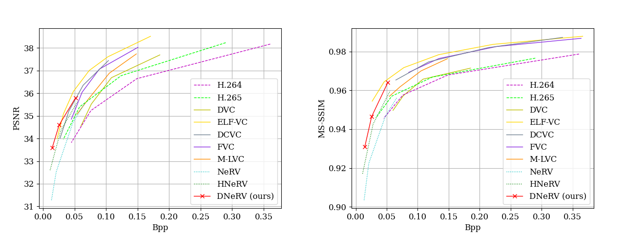
Figure 5: Compression results on 960 $\times$ 1920 UVG. DNeRV outperforms other INR-based methods.

video	regression				Inp-Mask-S		Inp-Mask-C
	NeRV	E-NeRV	HNeRV	DNeRV	HNeRV	DNeRV	HNeRV	DNeRV
Blackswan	28.48/0.812	29.38/0.867	30.35/0.891	30.92/0.913	26.51/0.825	29.01/0.886	24.64/0.783	27.45/0.858
Bmx-bumps	29.42/0.864	28.90/0.851	29.98/0.872	30.59/0.890	23.16/0.728	25.70/0.819	20.39/0.665	22.95/0.767
Bmx-trees	26.24/0.789	27.26/0.876	28.76/0.861	29.63/0.882	22.93/0.720	26.57/0.841	20.26/0.653	21.62/0.752
Breakdance	26.45/0.915	28.33/0.941	30.45/0.961	30.88/0.968	27.63/0.945	29.16/0.961	23.84/0.907	25.18/0.938
Camel	24.81/0.781	25.85/0.844	26.71/0.844	27.38/0.887	20.94/0.661	24.71/0.832	21.85/0.733	23.72/0.815
Car-round	24.68/0.857	26.01/0.912	27.75/0.912	29.35/0.937	23.96/0.752	27.63/0.854	22.06/0.810	24.82/0.886
Car-shadow	26.41/0.871	30.41/0.922	31.32/0.936	31.95/0.944	25.87/0.875	27.90/0.914	28.67/0.908	28.18/0.923
Car-turn	27.45/0.813	29.02/0.888	29.65/0.879	30.25/0.892	23.96/0.752	27.63/0.854	24.43/0.773	25.67/0.821
Cows	22.55/0.702	23.74/0.819	24.11/0.792	24.88/0.827	21.37/0.682	22.91/0.770	20.81/0.668	21.87/0.733
Dance-twril	25.79/0.797	27.07/0.864	28.19/0.845	29.13/0.870	23.05/0.743	26.13/0.830	21.10/0.704	23.00/0.783
Dog	28.17/0.795	30.40/0.882	30.96/0.898	31.32/0.905	25.34/0.739	27.43/0.824	23.09/0.677	24.96/0.763
Dog-ag	29.08/0.821	29.30/0.905	28.75/0.893	29.94/0.923	27.70/0.884	28.28/0.913	25.12/0.856	24.85/0.886
Drift-straight	26.65/0.860	29.10/0.941	30.80/0.932	31.50/0.940	24.79/0.833	27.00/0.892	20.15/0.725	22.61/0.823
Drift-turn	26.70/0.812	27.94/0.875	29.72/0.834	30.37/0.862	22.27/0.677	26.20/0.816	19.95/0.636	22.65/0.749
Goat	23.90/0.746	25.25/0.855	26.62/0.858	27.79/0.887	21.11/0.675	22.65/0.755	20.21/0.639	21.76/0.727
Libby	29.08/0.821	31.43/0.890	32.69/0.917	33.43/0.927	27.59/0.825	29.51/0.875	24.33/0.752	26.07/0.826
Mallard-fly	26.83/0.757	28.84/0.847	29.22/0.848	28.77/0.833	23.81/0.709	25.83/0.774	20.83/0.618	22.77/0.689
Mallard-water	25.20/0.824	27.28/0.896	29.08/0.908	29.69/0.922	23.55/0.803	24.11/0.845	21.18/0.743	21.15/0.796
Parkour	25.14/0.794	25.31/0.845	26.56/0.851	25.75/0.827	21.32/0.685	24.51/0.799	19.97/0.650	21.55/0.754
Rollerblade	29.28/0.898	33.32/0.964	32.19/0.935	32.49/0.940	29.32/0.911	30.41/0.931	27.31/0.901	27.63/0.917
Scooter-black	22.73/0.835	25.79/0.927	27.38/0.923	28.53/0.940	21.05/0.794	24.27/0.897	19.76/0.789	21.00/0.844
Stroller	29.28/0.859	30.37/0.914	31.31 0.894	32.73/0.928	25.90/0.796	28.46/0.876	22.86/0.734	24.52/0.822
Average	26.56/0.819	28.19/0.887	29.21/0.886	29.86/0.902	24.09/0.774	26.53/0.854	22.40/0.742	23.91/0.812

Table 2: Video regression and inpainting results on 960$\times$1920 Davis Dynamic in PSNR/SSIM, larger is better.

size of diff embedding	stage			params	PSNR/SSIM
	2	3	4
N/A				0.311M	29.64/0.908
				0.347M	29.95/0.914
$2\times 40\times 80$	A			0.288M	29.31/0.907
	A	C		0.339M	29.93/0.914
		C		0.339M	30.60/0.924
	A		C	0.348M	29.73/0.909
			C	0.348M	30.38/0.922
		C	C	0.348M	30.33/0.921
	A	C	C	0.348M	26.96/0.835
$2\times 10\times 20$		U		0.343M	29.66/0.907
Final		U		0.349M	30.80/0.930

Table 3: Ablation study for fusion module and diff embedding size, training on Bunny in 300 epochs. A indicates sum fusion, C is conv fusion and U is the CCU. The final version of DNeRV consists of diff embedding in shape of $2\times 40\times 80$, 3rd stage where merging and CCU as the fusion module. The first two rows which are marked as N/A represent HNeRV baseline, where the size of diff embedding is not available.

input of diff stream	conv fusion	CCU
$\Delta f(t)$	30.359/0.920	30.425/0.922
$\Delta f(t+1)$	30.354/0.919	-/-
$(\Delta f(t-1)+\Delta f(t+1))/2$	30.213/0.918	30.278/0.920
$\mathsf{concat}[\Delta f(t),\Delta f(t+1)]$	30.598/0.924	30.804/0.930
$\mathsf{concat}[\Delta f(t),\Delta f(t+1),\nabla f(t)]$	30.310/0.919	30.392/0.921

Table 4: Ablation study of various difference on Bunny in 0.35M and 300 epochs, where $\Delta$ is first order and $\nabla$ is second order difference.

5.2 Video Compression

We show the compression results in PSNR and SSIM on UVG dataset in Fig. 5. Without pruning and only 8 bits quantization with entropy encoding adopted, DNeRV outperforms other NeRV methods especially on PSNR. DNeRV optimizes the network structure under the condition of parameter amount, thus reducing the redundancy in weights. Although it couldn’t maintain performance in 40% pruning like [4, 21], the 10% pruned DNeRV is still competitive compared with other implicit methods. We also report VMAF [32] results on UVG in the appendix.

method	1920	params$\downarrow$	dec time$\downarrow$	FPS$\uparrow$
DCVC [19]	$\times$ 1080	35M	35590ms	0.028
Li 2022 [20]	$\times$ 1080	67M	525ms	1.9
Sheng 2021 [37]	$\times$ 1080	41M	470ms	2.12
HNeRV [1]	$\times$ 960	3.2M	30ms	33.3
DNeRV	$\times$ 960	3.5M	39ms	25.6

Table 5: Complexity comparison.

Compare with state-of-the-arts methods. We compare DNeRV with H.264 [48], H.265 [41], DVC [23], FVC [15], M-LVC [22], DCVC [19] and ELF-VC [33]. Without any specific modification, DNeRV is better than traditional video codecs H.264 or H.265 in both PSNR and SSIM, and it is also competitive with the state-of-the-art deep compression methods. We will explore the potential of DNeRV in video compression in the follow-up studies. The complexity comparison of video decoding with two rapid neural compression methods [20, 37] in model size, decoding time and FPS is shown in Tab 5.

5.3 Video Interpolation

Since the INR-based video representation is over-fitting to the given video, we evaluate the generalization of different methods by video interpolation task. We follow the setting in [1] and demonstrate the quantitative results on UVG in Tab. 6 and qualitative results in Fig. 6. Thanks to the consideration of adjacent dynamics, DNeRV outperforms other implicit methods especially on the videos owning dynamic scene and large motion. More results on DAVIS are reported in appendix.

Case study. Interpolation is quite challenging for the generalization ability of INRs. Shown in Tab.6, DNeRV earns 28.5% and 14.6% improvement against the best results on “Jockey” and “ReadySetGo”, where exist strong dynamics and large motion. Especially for “Jockey” in Fig. 6, we could recognize some numbers or letters from DNeRV’s prediction, but it’s impossible for HNeRV’s.

UVG	Beauty	Bospho	Honey	Jockey	Ready	Shake	Yacht	avg.
NeRV [4]	28.05	30.04	36.99	20.00	17.02	29.15	24.50	26.54
E-NeRV [21]	27.35	28.95	38.24	19.39	16.74	30.23	22.45	26.19
H-NeRV [1]	31.10	34.38	38.83	23.82	20.99	32.61	27.24	29.85
D-NeRV	35.99	35.19	37.43	30.61	24.05	35.34	28.70	32.47

Table 6: Video interpolation results on 960 $\times$ 1920 UVG in PSNR.

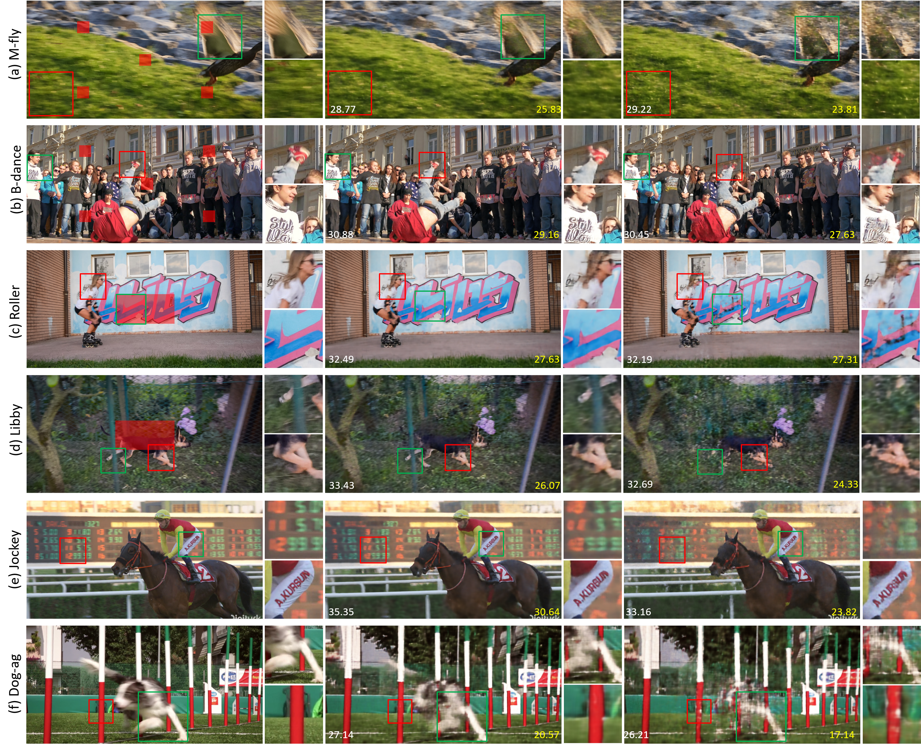
Figure 6: Visualization comparison for inpainting (a, b, c, d) and interpolation (e, f) results on Davis Dynamic. The left is ground truth, DNeRV’s results in mid and HNeRV’s on the right. White number is the best PSNR for each method training on original video, while yellow ones are testing PSNR on masked videos. Zoom in for details.

5.4 Video Inpainting

We conduct video inpainting experiments on DAVIS Dynamic with central mask and disperse mask. The central mask follows the setting in [52, 29] as the rectangular mask with width and height both 1/4 of the original frame. The disperse mask is five square masks in $100\times 100$ average distributed in fixed positions. The quantitative results are listed in Tab. 2 and qualitative performance is shown in Fig. 6. We train the implicit methods on raw videos but test them with masked videos. We only conduct the comparison with HNeRV because it beats other implicit methods on robust inpainting, reported in [1]. Although the diff is also masked before input, DNeRV still obtains impressive and robust results.

Case study. Detailed texture is a major difficulty for DNeRV to encode videos, because difference of neighboring frames is more like than high frequency details close to noise, such as “Mallard-fly” and “Cows”. However, DNeRV outperform other implicit methods in robustness and generalization. Although in “Mallard-fly”, DNeRV’s training PSNR is less than HNeRV, but severe trivial-fitting phenomenon happens. Those similar textures which in the same position among frames, seem as copies in HNeRV’s results, shown as (a, d) in Fig 6.

5.5 Ablation Study

We provide various ablation studies on Bunny with PSNR and MS-SSIM as the metrics, reported in Tab 3 and Tab. 4.

Diff stream. We compare the backward difference, forward difference, central difference and second order difference as input and merge one of them with content stream in 3rd stage. The results are shown in Tab. 4, indicating that higher-order difference may not be helpful for fitting. We concatenate both backward and forward difference as our default diff stream.

Param quantity. To verify the effectiveness of diff stream, we compare the hybrid ones without diff stream in varying model size (by changing the channels in decoder) with DNeRV. More parameters may not attributed to better performance. The params, converge speed and generalization ability should be balanced.

Diff embedding. The smaller shape of diff embedding would reduce both the model size and reconstruction quality. The shape in $2\times 40\times 80$ is adopted as default.

Fusion module. The ablation results reported in Tab 3 and Tab. 4 verify the effectiveness of proposed CCU. Compared with conv fusion or sum fusion, CCU improves PSNR by adaptively merging two-stream features.

Fusion stages. It is vital for DNeRV to select the stage where two streams are merged, we do ablations on every possible connection. Decoder should balance the params and the difficulty of gradient descent. DNeRV adopts merging in 3rd stage without sum fusion. Further we upgrade conv fusion to CCU.

6 Conclusion

In this paper, we propose the difference neural representation for videos (DNeRV) for modeling the inherent dynamics of contextual frames. Relying on the diff stream and collaborative content unit, DNeRV retains its advantages in reconstruction quality for video regression, compression, inpainting and interpolation. Consequently, the experimental results show that the proposed DNeRV could achieve effective and robust representation for videos by achieving a better approximation to the implicit mapping than existing NeRV methods.

Future directions. DNeRV shows its potential on various visual tasks. The improved task-specific approach based on DNeRV is promising to challenge the state-of-the-art methods. Also, rigorous theoretical analysis needs to be improved for INR-based networks $g_{\theta}$ fitting the continuous $f$ on finite training tuple via gradient descent.

Acknowledgements. We thank Xingyu Xie for comments that greatly improved the manuscript. The work was supported in part by National Key Research and Development Project of China (2022YFF0902402).

Appendix

7 Implementation Details

7.1 Architecture of diff encoder

The strides in diff encoder depends on the resolution of input frame and the size of output diff embeddings, shown as Tab. 7.

size of diff embeddings	resolution	strides
2 $\times$ 40 $\times$ 80	640 $\times$ 1280	(2,2,2,2)
	480 $\times$ 960	(3,2,2)
	960 $\times$ 1920	(4,3,2)
2 $\times$ 10 $\times$ 20	960 $\times$ 1920	(4,4,3,2)

Table 7: Architecture of diff encoder.

7.2 Architecture of decoder

The architecture of decoders with CCU in different size is given in Tab. 8. $C_{init}$ is the initial channel width of embeddings before feeding to decoder stages. Once feeding the $w_{0}\times h_{0}\times C_{init}$ embeddings into following stage, for example Stage 1 with stride $s=5$, the size of output feature maps is $5w_{0}\times 5h_{0}\times C_{1}$, where $C_{1}=\lfloor C_{init}/r\rfloor$ is the output channel width of Stage 1, $r=1.2$ is the reduction rate for each stage and $\lfloor x\rfloor$ is the round down operator. $K_{c}$ is the kernel size in CCU. The minimal and maximal kernel size in different decoder stages are 1 and 5, follow the setting in [1].

resolution	size	$C_{0}$	$C_{init}$	$C_{1}$	$C_{5}$	strides	$K_{c}$
640 $\times$ 1280	0.35	16	32	26	11	(5,4,4,2,2)	3
	0.75	16	48	40	18	(5,4,4,2,2)	3
	1.5	16	68	56	25	(5,4,4,2,2)	3
	3	16	95	79	37	(5,4,4,2,2)	3
480 $\times$ 960	3	16	110	91	42	(5,4,3,2,2)	1
960 $\times$ 1920	1.58	16	68	56	25	(5,4,4,3,2)	1
	3	16	92	76	35	(5,4,4,3,2)	1

Table 8: Architecture of decoder and CCU.

7.3 Experimental Details

In video compression, the network structure would be adjusted for different sizes and bpp, 1.58M with diff embedding in $2\times 10\times 20$ for 0.0146 bpp, 3M with diff embedding in $2\times 10\times 20$ for 0.0257 bpp and 3M with diff embedding in $2\times 40\times 80$ for 0.0517 bpp.

8 Additional quantitative results

8.1 Comparison for video interpolation on DAVIS Dynamic

Interpolation results between different methods on DAVIS Dynamic are shown in Tab. 12. We only compare DNeRV with hybrid-based implicit methods [1] because HNeRV is the current best implicit method for video representation.

8.2 The effects of different compression techniques

Ablations for various compression technique on UVG is given in Tab. 11. In future work, more advanced model compression methods would be used on the NeRV methods owing to the fewer redundance in the weights.

8.3 The effects of different compression techniques

For the evaluation of video compression, the results of VMAF [32] are demonstrated in Tab. 9.

Bpp	Beauty	Bospho	Honey	Jockey	Ready	Shake	Yacht	avg.
0.015	77.74	71.43	93.71	68.02	53.55	80.74	57.55	71.82
0.025	83.78	78.18	93.16	75.38	60.97	82.53	63.45	76.78
0.05	85.15	77.45	94.22	84.02	67.47	86.13	60.09	79.22

Table 9: Number of VMAF on 960 $\times$ 1920 UVG in different Bpp.

8.4 Ablation results for optimizer

Results for optimizer ablations on Bunny with 0.35M size and 300 epochs is given in Tab. 10. Adan [50] is much more effective than Adam for larger learning rate.

learning rate	optimizer	50	100	150	200	250	300
5e-4	Adam	24.97/0.769	27.86/0.873	28.99/0.905	30.10/0.920	30.66/0.926	30.80/0.927
	Adan	24.17/0.734	26.42/0.823	27.65/0.862	28.41/0.881	28.80/0.890	28.91/0.893
1e-3	Adam	26.36/0.829	24.67/0.776	27.06/0.841	27.71/0.863	28.46/0.876	28.56/0.878
	Adan	25.53/0.789	28.23/0.879	29.31/0.905	30.03/0.917	30.40/0.922	30.50/0.924
3e-3	Adam	18.39/0.519	18.81/0.548	19.31/0.584	19.18/0.583	19.32/0.591	19.36/0.594
	Adan	27.59/0.865	29.76/0.918	30.59/0.933	31.35/0.941	31.78/0.944	31.89/0.946

Table 10: Optimizer ablations on Bunny in PSNR/SSIM.

UVG	Beauty	Bospho	Honey	Jockey	Ready	Shake	Yacht
N/A	40.00/0.972	36.67/0.965	41.92/0.993	35.75/0.947	28.68/0.917	36.53/0.962	31.10/0.924
8-bit Quant	39.97/0.972	36.64/0.965	41.20/0.993	35.73/0.947	28.66/0.916	36.35/0.961	31.00/0.923
8-bit Quant + Pruning (10%)	39.38/0.971	36.41/0.964	39.95/0.991	35.50/0.946	28.55/0.915	35.42/0.959	30.78/0.921
8-bit Quant + Pruning (20%)	33.72/0.961	34.56/0.957	34.47/0.978	32.25/0.938	27.63/0.905	28.66/0.943	28.84/0.908

Table 11: Compression ablations on UVG in PSNR/SSIM.

Videos	DNeRV		HNeRV
	test	train	test	train
Blackswan	23.89/0.712	28.98/0.874	21.67/0.589	28.76/0.865
Bmx-bumps	22.34/0.696	25.96/0.784	19.24/0.549	30.32/0.883
Camel	21.31/0.656	23.79/0.761	20.69/0.586	26.28/0.855
Breakdance	22.28/0.858	27.26/0.937	20.40/0.841	29.53/0.958
Car-round	20.42/0.725	28.91/0.931	16.92/0.560	28.23/0.919
Bmx-trees	21.68/0.644	28.88/0.867	18.39/0.453	28.99/0.872
Car-shadow	22.47/0.734	29.41/0.913	19.35/0.622	28.64/0.897
Cows	20.89/0.629	25.24/0.837	20.45/0.590	24.71/0.815
Dance-twirl	20.95/0.656	29.19/0.872	18.38/0.517	28.70/0.857
Dog	24.91/0.683	29.55/0.857	21.99/0.457	29.85/0.868
Car-turn	24.29/0.737	28.21/0.838	22.34/0.654	27.80/0.828
Dog-agility	20.57/0.730	27.14/0.852	17.14/0.609	26.21/0.818
Drift-straight	19.11/0.645	29.75/0.921	15.62/0.354	29.72/0.916
Drift-turn	21.22/0.649	29.45/0.849	18.44/0.501	28.43/0.815
Goat	20.46/0.554	28.63/0.908	18.22/0.327	27.69/0.891
Libby	24.24/0.688	32.22/0.906	20.00/0.472	30.75/0.871
Mallard-fly	21.81/0.610	28.25/0.809	19.23/0.397	27.26/0.788
Mallard-water	21.24/0.687	27.55/0.882	17.60/0.429	29.23 0.911
Parkour	22.13/0.680	27.32/0.879	18.82/0.488	26.77/0.863
Rollerblade	24.91/0.850	30.52/0.915	21.56/0.782	29.92/0.907
Scooter-black	17.15/0.633	27.26/0.926	14.37/0.416	26.33/0.901
Stroller	23.32/0.718	32.36/0.923	20.47/0.559	31.68/0.905
Average	21.89/0.690	28.45/0.875	19.15/0.534	28.44/0.873

Table 12: Interpolation results on DAVIS Dynamic.

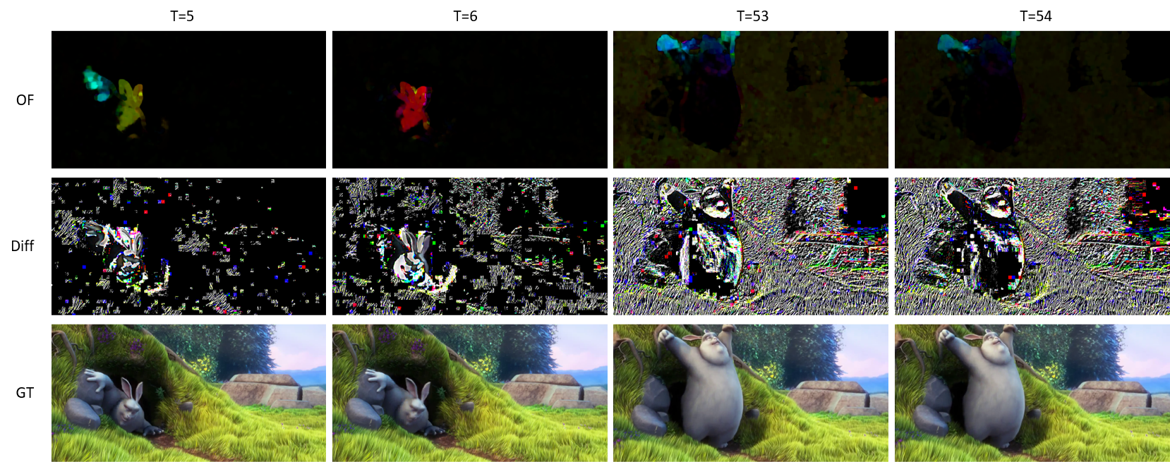
Figure 7: Comparison between optical flow and difference stream.

9 Additional qualitative results

9.1 Visualization of video interpolation on UVG

Additional interpolation comparison on UVG is given in Fig. 8 and Fig. 9.

“Jockey” and “ReadySetGo” are two typical videos with large motion and dynamic scenes from UVG. In Fig. 8 and Fig. 9, we could find that the interpolations generated by DNeRV are obviously better than HNeRV. Some subtle spatial structures in interpolations of DNeRV, such as numbers on the screen or flagpole in the distance, remain nearly constant between adjacent frames.

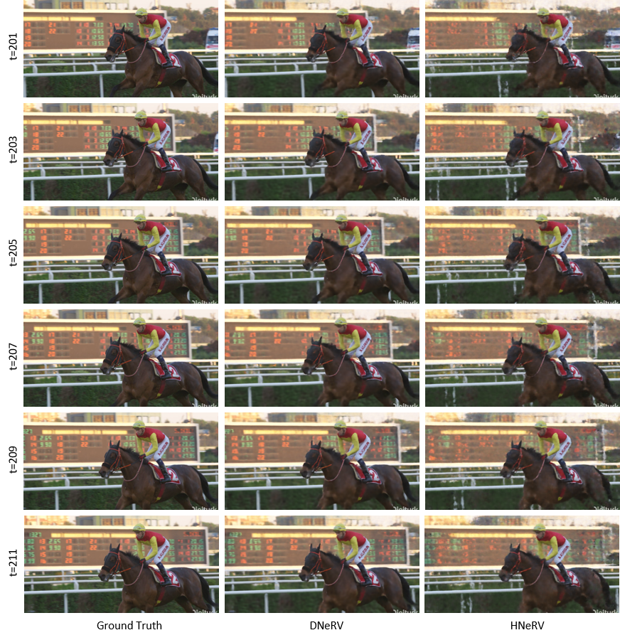
Figure 8: Additional examples for video interpolation on Jockey.

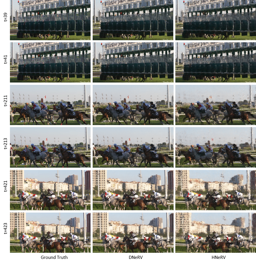
Figure 9: Additional examples for video interpolation on ReadySetGo.

9.2 Visualization of video interpolation on DAVIS Dynamic

Additional interpolation comparison on DAVIS Dynamic is given in Fig. 10, Fig. 11, Fig. 12 and Fig. 13.

DAVIS Dynamic is more difficult than UVG by reason of more dynamic scene changing and fewer frames. Although DNeRV outperforms HNeRV achieving the best results of implicit methods, but there is still much room for improvement. Once increasing the parameter quantity and utilizing task-specific modification, DNeRV could be competitive with state-of-the-art deep interpolation methods.

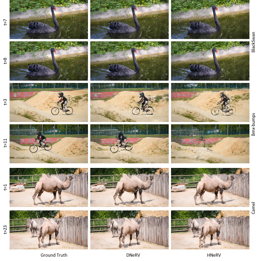
Figure 10: Additional examples for video interpolation on Blackswan, Bmx-bumps and Camel.

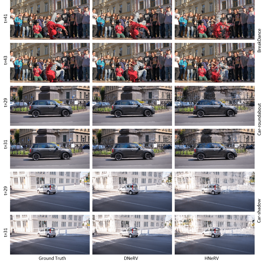
Figure 11: Additional examples for video interpolation on Breakdance, Car-roundabout and Car-shadow.

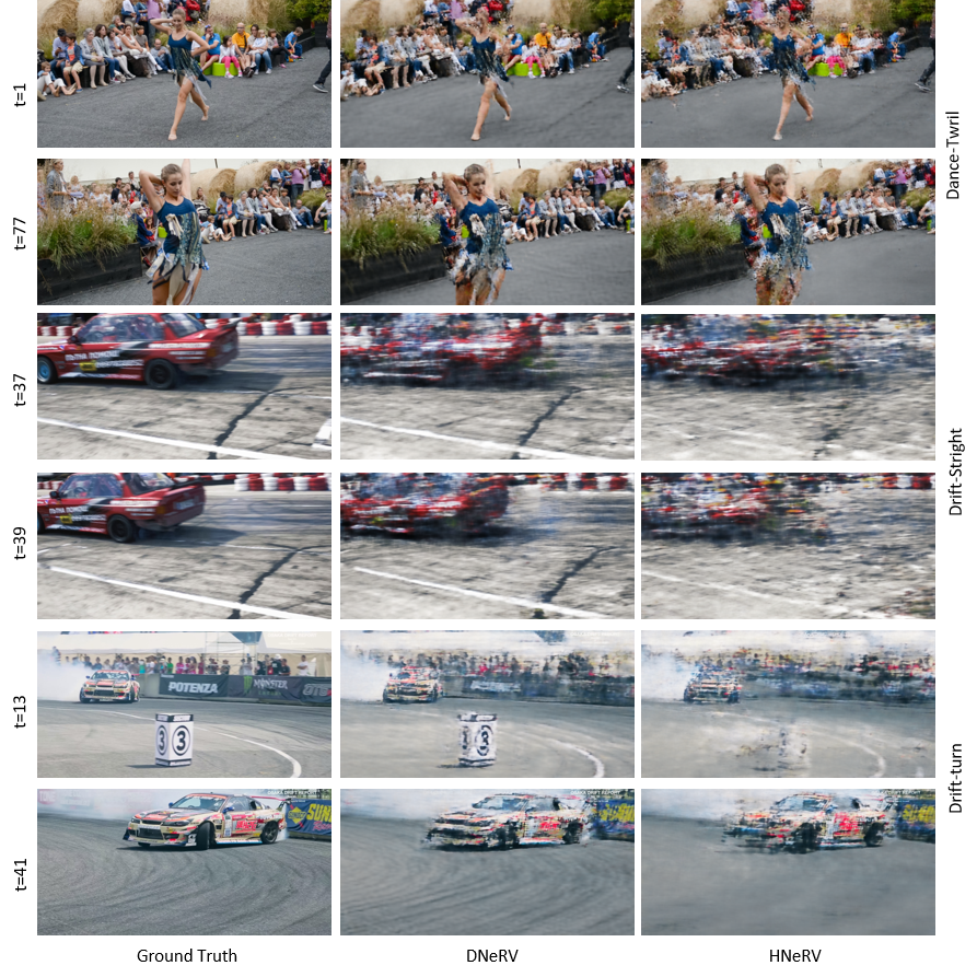
Figure 12: Additional examples for video interpolation on Dance-twril, Drift-straight and Drift-turn.

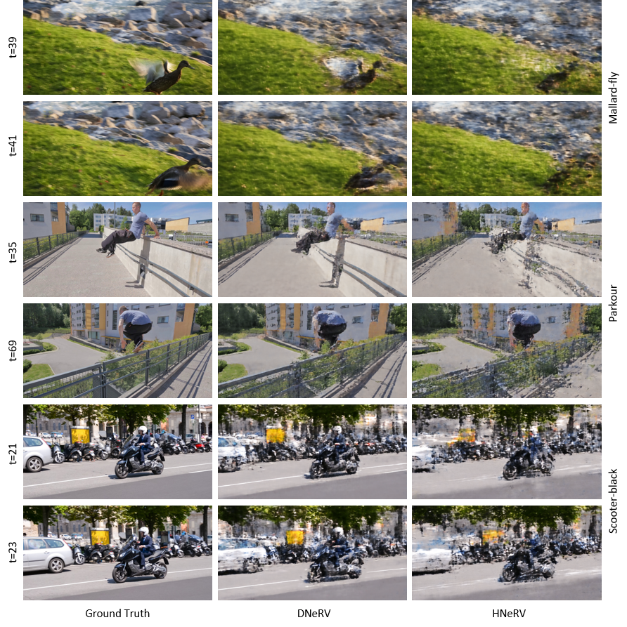
Figure 13: Additional examples for video interpolation on Mallard-fly, Parkour and Scooter-black.

9.3 Visualization of video inpainting on DAVIS Dynamic

Additional inpainting comparison on DAVIS Dynamic is shown in Fig. 14, Fig. 15 and Fig. 16.

Due to diff stream and CCU, DNeRV could model different regions of the frame more robustly, reduce the influence of masked regions. Besides, one limitation of DNeRV is that it couldn’t model the detail texture well, and we will improve it in the future work.

9.4 Visualization of optical flow and difference stream

We conducted additional experiments on Bunny, following the same setting as Tab. 1(a). The PSNR results are 29.13, 29.25, 28.84, and 28.70 in dB for the model sizes of 0.35M, 0.75M, 1.5M, and 3M. The optical flow is computed using Gunner Farneback algorithm by opencv-python 4.5.3 and numpy 1.19.5.

The visualization comparison between optical flow and diff stream is shown in Fig. 7. It can be clearly observed that, although optical flow contains motion information, it loses huge other information in pixel domain. Saliency motion information in optical flow may be key in action recognition or motion prediction, but it cannot bring much help for pixel-level reconstruction tasks. For example, the fluctuation of grass or the change of skin brightness with the light may not help to recognize the rabbit’s movements, but they are essential for reconstruction. Diff stream records all these information in unbiased way.

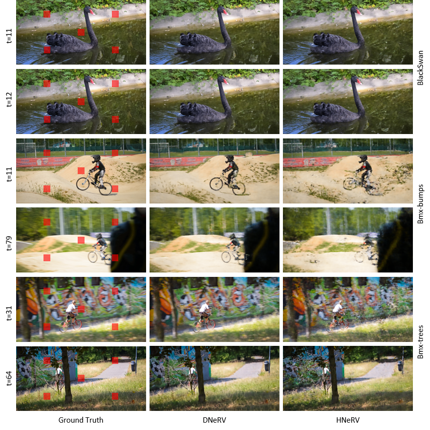
Figure 14: Additional examples for video interpolation on Blackswan, Bmx-bumps and Bmx-trees.

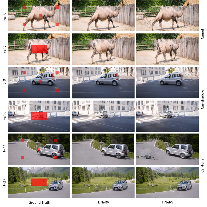
Figure 15: Additional examples for video interpolation on Camel, Car-shadow and Car-turn.

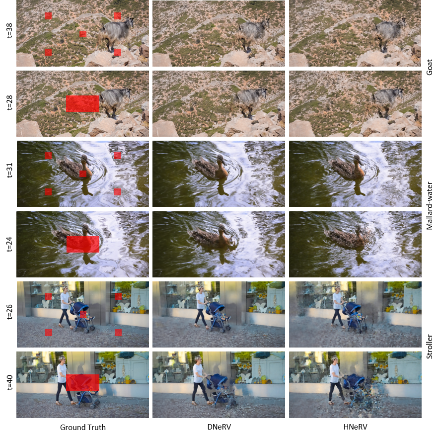
Figure 16: Additional examples for video interpolation on Goat, Mallard-water and Stroller.

References

- [1] Anonymous. Hnerv: A hybrid neural representation for videos. 2022.
- [2] Emmanuel J. Candès and Terence Tao. Decoding by linear programming. IEEE Transactions on Information Theory, 2005.
- [3] João Carreira and Andrew Zisserman. Quo vadis, action recognition? A new model and the kinetics dataset. In 2017 IEEE Conference on Computer Vision and Pattern Recognition, CVPR 2017, 2017.
- [4] Hao Chen, Bo He, Hanyu Wang, Yixuan Ren, Ser-Nam Lim, and Abhinav Shrivastava. Nerv: Neural representations for videos. In NeurIPS, 2021.
- [5] Zeyuan Chen, Yinbo Chen, Jingwen Liu, Xingqian Xu, Vidit Goel, Zhangyang Wang, Humphrey Shi, and Xiaolong Wang. Videoinr: Learning video implicit neural representation for continuous space-time super-resolution. In IEEE/CVF Conference on Computer Vision and Pattern Recognition, CVPR 2022, 2022.
- [6] Zhiqin Chen and Hao Zhang. Learning implicit fields for generative shape modeling. In IEEE Conference on Computer Vision and Pattern Recognition, CVPR 2019, 2019.
- [7] Junyoung Chung, Caglar Gülcehre, Kyunghyun Cho, and Yoshua Bengio. Empirical evaluation of gated recurrent neural networks on sequence modeling. arXiv:1412.3555, 2014.
- [8] Zhiwen Fan, Yifan Jiang, Peihao Wang, Xinyu Gong, Dejia Xu, and Zhangyang Wang. Unified implicit neural stylization. In ECCV 2022, 2022.
- [9] Rizal Fathony, Anit Kumar Sahu, Devin Willmott, and J. Zico Kolter. Multiplicative filter networks. In 9th International Conference on Learning Representations, ICLR 2021, 2021.
- [10] Christoph Feichtenhofer, Axel Pinz, and Andrew Zisserman. Convolutional two-stream network fusion for video action recognition. In 2016 IEEE Conference on Computer Vision and Pattern Recognition, CVPR 2016, 2016.
- [11] Jonathan Frankle and Michael Carbin. The lottery ticket hypothesis: Finding sparse, trainable neural networks. arXiv: Learning, 2019.
- [12] Amir Gholami, K. Kwon, Bichen Wu, Zizheng Tai, Xiangyu Yue, Peter H. Jin, Sicheng Zhao, and Kurt Keutzer. Squeezenext: Hardware-aware neural network design. 2018 IEEE/CVF Conference on Computer Vision and Pattern Recognition Workshops (CVPRW), 2018.
- [13] Albert Gu, Çaglar Gülçehre, Thomas Paine, Matt Hoffman, and Razvan Pascanu. Improving the gating mechanism of recurrent neural networks. In Proceedings of the 37th International Conference on Machine Learning, ICML 2020, pages 3800–3809.
- [14] Sepp Hochreiter and Jürgen Schmidhuber. Long short-term memory. Neural Comput., 1997.
- [15] Zhihao Hu, Guo Lu, and Dong Xu. Fvc: A new framework towards deep video compression in feature space. 2021 IEEE/CVF Conference on Computer Vision and Pattern Recognition (CVPR), 2021.
- [16] Zhewei Huang, Tianyuan Zhang, Wen Heng, Boxin Shi, and Shuchang Zhou. Real-time intermediate flow estimation for video frame interpolation. In Proceedings of the European Conference on Computer Vision (ECCV), 2022.
- [17] Diederik P. Kingma and Jimmy Ba. Adam: A method for stochastic optimization. In 3rd International Conference on Learning Representations, ICLR 2015, 2015.
- [18] Janus B. Kristensen. Big buck bunny. 2010.
- [19] Jiahao Li, Bin Li, and Yan Lu. Deep contextual video compression. 2021.
- [20] Jiahao Li, Bin Li, and Yan Lu. Hybrid spatial-temporal entropy modelling for neural video compression. In MM ’22: The 30th ACM International Conference on Multimedia, 2022.
- [21] Zizhang Li, Mengmeng Wang, Huaijin Pi, Kechun Xu, Jianbiao Mei, and Yong Liu. E-nerv: Expedite neural video representation with disentangled spatial-temporal context. arXiv:2207.08132, 2022.
- [22] Jianping Lin, Dong Liu, Houqiang Li, and Feng Wu. M-lvc: Multiple frames prediction for learned video compression. 2020 IEEE/CVF Conference on Computer Vision and Pattern Recognition (CVPR), 2020.
- [23] Guo Lu, Wanli Ouyang, Dong Xu, Xiaoyun Zhang, Chunlei Cai, and Zhiyong Gao. Dvc: An end-to-end deep video compression framework. 2019.
- [24] Li Ma, Xiaoyu Li, Jing Liao, Qi Zhang, Xuan Wang, Jue Wang, and Pedro V. Sander. Deblur-nerf: Neural radiance fields from blurry images. In IEEE/CVF Conference on Computer Vision and Pattern Recognition, CVPR 2022, 2022.
- [25] Long Mai and Feng Liu. Motion-adjustable neural implicit video representation. In IEEE/CVF Conference on Computer Vision and Pattern Recognition, CVPR 2022, 2022.
- [26] Alexandre Mercat, Marko Viitanen, and Jarno Vanne. UVG dataset: 50/120fps 4k sequences for video codec analysis and development. In Proceedings of the 11th ACM Multimedia Systems Conference, MMSys 2020, 2020.
- [27] Ben Mildenhall, Peter Hedman, Ricardo Martin-Brualla, Pratul P. Srinivasan, and Jonathan T. Barron. Nerf in the dark: High dynamic range view synthesis from noisy raw images. In IEEE/CVF Conference on Computer Vision and Pattern Recognition, CVPR 2022, 2022.
- [28] Ben Mildenhall, Pratul P. Srinivasan, Matthew Tancik, Jonathan T. Barron, Ravi Ramamoorthi, and Ren Ng. Nerf: Representing scenes as neural radiance fields for view synthesis. In Proceedings of the European Conference on Computer Vision (ECCV), 2020.
- [29] Hao Ouyang, Tengfei Wang, and Qifeng Chen. Internal video inpainting by implicit long-range propagation. 2021 IEEE/CVF International Conference on Computer Vision (ICCV), 2021.
- [30] Federico Perazzi, Jordi Pont-Tuset, Brian McWilliams, Luc Van Gool, Markus H. Gross, and Alexander Sorkine-Hornung. A benchmark dataset and evaluation methodology for video object segmentation. In 2016 IEEE Conference on Computer Vision and Pattern Recognition, CVPR 2016, 2016.
- [31] Albert Pumarola, Enric Corona, Gerard Pons-Moll, and Francesc Moreno-Noguer. D-nerf: Neural radiance fields for dynamic scenes. In IEEE Conference on Computer Vision and Pattern Recognition, CVPR 2021, 2021.
- [32] Reza Rassool. Vmaf reproducibility: Validating a perceptual practical video quality metric. 2017 IEEE International Symposium on Broadband Multimedia Systems and Broadcasting (BMSB), 2017.
- [33] Oren Rippel, Alexander G. Anderson, Kedar Tatwawadi, Sanjay Nair, Craig Lytle, and Lubomir D. Bourdev. Elf-vc: Efficient learned flexible-rate video coding. 2021 IEEE/CVF International Conference on Computer Vision (ICCV), 2021.
- [34] Johannes Schmidt-Hieber. Nonparametric regression using deep neural networks with relu activation function. ArXiv, abs/1708.06633, 2020.
- [35] Laura Sevilla-Lara, Yiyi Liao, Fatma Güney, Varun Jampani, Andreas Geiger, and Michael J. Black. On the integration of optical flow and action recognition. In Pattern Recognition - 40th German Conference, GCPR, 2018.
- [36] Wentao Shangguan, Yu Sun, Weijie Gan, and Ulugbek S. Kamilov. Learning cross-video neural representations for high-quality frame interpolation. In Proceedings of the European Conference on Computer Vision (ECCV), 2022.
- [37] Xihua Sheng, Jiahao Liu Li, Bin Li, Li Li, Dong Liu, and Yan Lu. Temporal context mining for learned video compression. arXiv:2111.13850, 2022.
- [38] Karen Simonyan and Andrew Zisserman. Two-stream convolutional networks for action recognition in videos. In NeurIPS, 2014.
- [39] Vincent Sitzmann, Julien N. P. Martel, Alexander W. Bergman, David B. Lindell, and Gordon Wetzstein. Implicit neural representations with periodic activation functions. In NeurIPS, 2020.
- [40] Yannick Strümpler, Janis Postels, Ren Yang, Luc Van Gool, and Federico Tombari. Implicit neural representations for image compression. In ECCV, 2022.
- [41] Gary J. Sullivan, Jens-Rainer Ohm, Woojin Han, and Thomas Wiegand. Overview of the high efficiency video coding (HEVC) standard. IEEE Trans. Circuits Syst. Video Technol., 2012.
- [42] Deqing Sun, Xiaodong Yang, Ming-Yu Liu, and Jan Kautz. Pwc-net: Cnns for optical flow using pyramid, warping, and cost volume. In 2018 IEEE Conference on Computer Vision and Pattern Recognition, CVPR, 2018.
- [43] Matthew Tancik, Pratul P. Srinivasan, Ben Mildenhall, Sara Fridovich-Keil, Nithin Raghavan, Utkarsh Singhal, Ravi Ramamoorthi, Jonathan T. Barron, and Ren Ng. Fourier features let networks learn high frequency functions in low dimensional domains. In NeurIPS, 2020.
- [44] Ruben Villegas, Jimei Yang, Seunghoon Hong, Xunyu Lin, and Honglak Lee. Decomposing motion and content for natural video sequence prediction. In 5th International Conference on Learning Representations, ICLR 2017, 2017.
- [45] Yunbo Wang, Zhifeng Gao, Mingsheng Long, Jianmin Wang, and Philip S. Yu. Predrnn++: Towards A resolution of the deep-in-time dilemma in spatiotemporal predictive learning. In Proceedings of the 35th International Conference on Machine Learning, ICML 2018, 2018.
- [46] Yunbo Wang, Mingsheng Long, Jianmin Wang, Zhifeng Gao, and Philip S. Yu. Predrnn: Recurrent neural networks for predictive learning using spatiotemporal lstms. In NeurIPS, 2017.
- [47] Zhou Wang, Eero P. Simoncelli, and Alan Conrad Bovik. Multiscale structural similarity for image quality assessment. The Thrity-Seventh Asilomar Conference on Signals, Systems & Computers, 2003, 2003.
- [48] Thomas Wiegand, Gary J. Sullivan, Gisle Bjøntegaard, and Ajay Luthra. Overview of the H.264/AVC video coding standard. IEEE Trans. Circuits Syst. Video Technol., 2003.
- [49] Xingyu Xie, Hao Kong, Jianlong Wu, Wayne Zhang, Guangcan Liu, and Zhouchen Lin. Maximum-and-concatenation networks. 2020.
- [50] Xingyu Xie, Pan Zhou, Huan Li, Zhouchen Lin, and Shuicheng Yan. Adan: Adaptive nesterov momentum algorithm for faster optimizing deep models. ArXiv, abs/2208.06677, 2022.
- [51] Qiangeng Xu, Zexiang Xu, Julien Philip, Sai Bi, Zhixin Shu, Kalyan Sunkavalli, and Ulrich Neumann. Point-nerf: Point-based neural radiance fields. In IEEE/CVF Conference on Computer Vision and Pattern Recognition, CVPR 2022, 2022.
- [52] Rui Xu, Xiaoxiao Li, Bolei Zhou, and Chen Change Loy. Deep flow-guided video inpainting. 2019 IEEE/CVF Conference on Computer Vision and Pattern Recognition (CVPR), 2019.
- [53] Sihyun Yu, Jihoon Tack, Sangwoo Mo, Hyunsu Kim, Junho Kim, Jung-Woo Ha, and Jinwoo Shin. Generating videos with dynamics-aware implicit generative adversarial networks. In The Tenth International Conference on Learning Representations, ICLR 2022, 2022.
- [54] Wei Yu, Yichao Lu, Steve Easterbrook, and Sanja Fidler. Efficient and information-preserving future frame prediction and beyond. In 8th International Conference on Learning Representations, ICLR 2020, 2020.
- [55] Gizem Yüce, Guillermo Ortiz-Jiménez, Beril Besbinar, and Pascal Frossard. A structured dictionary perspective on implicit neural representations. In IEEE/CVF Conference on Computer Vision and Pattern Recognition, CVPR 2022, 2022.
- [56] Lu Zhang, Ju Dai, Huchuan Lu, You He, and Gang Wang. A bi-directional message passing model for salient object detection. In 2018 IEEE Conference on Computer Vision and Pattern Recognition, CVPR 2018, 2018.
- [57] Long Zhao, Xi Peng, Yu Tian, Mubbasir Kapadia, and Dimitris N. Metaxas. Learning to forecast and refine residual motion for image-to-video generation. In Proceedings of the European Conference on Computer Vision (ECCV), 2018.
- [58] Shuaifeng Zhi, Tristan Laidlow, Stefan Leutenegger, and Andrew J. Davison. In-place scene labelling and understanding with implicit scene representation. In ICCV, 2021.