Soliton Gas: Theory, Numerics and Experiments

Abstract

The concept of soliton gas was introduced in 1971 by V. Zakharov as an infinite collection of weakly interacting solitons in the framework of Korteweg-de Vries (KdV) equation. In this theoretical construction of a diluted soliton gas, solitons with random parameters are almost non-overlapping. More recently, the concept has been extended to dense gases in which solitons strongly and continuously interact. The notion of soliton gas is inherently associated with integrable wave systems described by nonlinear partial differential equations like the KdV equation or the one-dimensional nonlinear Schrödinger equation that can be solved using the inverse scattering transform. Over the last few years, the field of soliton gases has received a rapidly growing interest from both the theoretical and experimental points of view. In particular, it has been realized that the soliton gas dynamics underlies some fundamental nonlinear wave phenomena such as spontaneous modulation instability and the formation of rogue waves. The recently discovered deep connections of soliton gas theory with generalized hydrodynamics have broadened the field and opened new fundamental questions related to the soliton gas statistics and thermodynamics. We review the main recent theoretical and experimental results in the field of soliton gas. The key conceptual tools of the field, such as the inverse scattering transform, the thermodynamic limit of finite-gap potentials and the Generalized Gibbs Ensembles are introduced and various open questions and future challenges are discussed.

I Introduction

Random nonlinear waves in dispersive media have been the subject of intense research in nonlinear physics for more than half a century, most notably in the contexts of water wave dynamics and nonlinear optics. A significant portion of the work in this area has been centred around wave turbulence—the theory of out of equilibrium random weakly nonlinear dispersive waves in non-integrable systems Zakharov et al. (1992); Nazarenko (2011a). One of the most important results of the wave turbulence theory is the analytical determination in Zakharov (1965) of the power-law Fourier spectra analogous to the Kolmogorov spectra describing energy flux through scales in dissipative hydrodynamic turbulence.

More recently, a new theme in turbulence theory has emerged in connection with the dynamics of strongly nonlinear random waves described by integrable systems such as the Korteweg-de Vries (KdV) and 1D nonlinear Schrödinger (NLS) equations. This kind of random wave motion in nonlinear conservative systems, dubbed integrable turbulence Zakharov (2009), has attracted significant attention from both fundamental and applied perspectives. The interest in integrable turbulence is motivated by the inherent randomness of many real-life systems (due to random initial and boundary conditions or to complex interaction mechanisms) even though the underlying physical models may be amenable to the well-established mathematical techniques of integrable systems theory such as the inverse scattering transform or finite-gap theory Novikov et al. (1984); Osborne (2010).

The integrable turbulence framework is particularly pertinent to the description of modulationally unstable systems which can exhibit highly complex nonlinear behaviours that can be adequately described in terms of the turbulence theory concepts such as probability distribution functions, ensemble averages, Fourier spectra etc. Agafontsev and Zakharov (2015, 2016); Randoux et al. (2016); Kraych et al. (2019); Copie et al. (2020); Suret et al. (2016). We stress that the term ‘turbulence’ in this context is understood as complex spatiotemporal dynamics that require probabilistic description and are not related to the energy cascades through scales, the prime feature of strong hydrodynamic and weak wave turbulence.

Along with the fundamental, conceptual significance, the physical relevance of integrable turbulence is supported by recent laboratory experiments Walczak et al. (2015); Suret et al. (2016); Närhi et al. (2016); Tikan et al. (2018); Redor et al. (2020); Suret et al. (2020); Lebel et al. (2021) and observations of natural wave phenomena, e.g. in ocean waves Costa et al. (2014); Osborne et al. (2019a).

The main tool for the analysis of integrable nonlinear dispersive partial differential equations (PDEs) is the Inverse Scattering Transform (IST) Gardner et al. (1967) which is based on the reformulation of a nonlinear PDE as a compatibility condition of two linear problems (the so-called Lax pair): a stationary spectral (scattering) problem and an evolution problem—for the same auxiliary function. Within the classical IST setting, formulated for the wave fields decaying sufficiently rapidly as $|x|\to\infty$ the scattering spectrum consists of two components: discrete and continuous, corresponding to two contrasting types of the wave motion: solitary waves (solitons) and dispersive radiation respectively. Importantly, integrable evolution preserves the IST spectrum in time.

Localized nonlinear solitary waves, termed solitons in the context of integrable systems, are a ubiquitous and fundamental feature of nonlinear dispersive wave propagation. They exhibit particle-like properties such as elastic, pairwise interactions accompanied by certain phase/position shifts Zabusky and Kruskal (1965) and have been extensively studied both theoretically Ablowitz et al. (1974); Novikov et al. (1984); Newell (1985) and experimentally Remoissenet (2013). The particle-like properties of solitons suggest some natural questions pertaining to the realm of statistical mechanics, e.g. one can consider a soliton gas as an infinite ensemble of interacting solitons characterised by random amplitude and phase distributions. Then, given the properties of the elementary, ‘microscopic’, soliton interactions the next natural step is the determination of the emergent, out of equilibrium macroscopic dynamics (i.e. hydrodynamics or kinetics) of a soliton gas.

Due to the presence of an infinite number of conserved quantities, integrable systems do not reach the thermodynamic equilibrium state characterized by the so-called Rayleigh-Jeans distribution of the modes (equipartition of energy). Consequently, the properties of soliton gases will be very different compared to the properties of classical gases whose particle interactions are non-elastic. Additionally, the particle-wave duality of solitons implies that hydrodynamic description of a soliton gas should be complemented by the characterisation of the associated nonlinear turbulent wave field in terms of the probability density function, power spectrum, correlations etc. It has transpired recently that soliton gas dynamics are instrumental in the understanding of a number of important statistical nonlinear wave phenomena such as spontaneous modulational instability and the rogue wave formation in one-dimensional wave propagation Gelash et al. (2019).

One can distinguish two basic mechanisms of the ‘spontaneous’, uncontrollable generation of a soliton gas. One mechanism involves the process of soliton fission, where statistical soliton ensembles emerge as the asymptotic outcome of long-time evolution of the so-called ‘partially coherent waves’, which can be viewed as collections of randomly distributed broad pulses, see Fig. 1 and Refs. Walczak et al. (2015); Suret et al. (2016); Tikan et al. (2018). Alternatively, soliton ensembles can be initially generated from a non-random (e.g. periodic) signal and then undergo effective randomization due to elastic reflections from the boundaries and subsequent multiple collisions, see Redor et al. (2020) for the example of the soliton gas generation in a shallow-water wave tank. The second mechanism of the soliton gas generation is related to the already mentioned phenomenon of modulational instability, where the basic coherent nonlinear mode of an unstable system—the plane wave—is subjected to a random perturbation (a noise), resulting in the development of large-amplitude small-scale fluctuations of the wave field and the establishment at $t\to\infty$ of a stationary integrable turbulence Agafontsev and Zakharov (2015). It was shown in Gelash et al. (2019) that for the wave systems described by the focusing nonlinear Schrödinger (fNLS) equation such integrable turbulence exhibits the properties of a dense bound-state (non-propagating) soliton gas.

Soliton gas can also be synthesized in a controllable manner directly, e.g. by programming a water tank wavemaker according to the IST-prescribed random multi-soliton solution of the relevant integrable equation, see Suret et al. (2020).

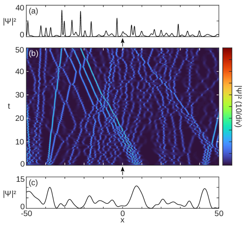
Figure 1: Emergence of soliton gas in the long-time evolution of a partially coherent wave $\psi(x,t)$ in the focusing NLS equation (equation (6) with $\sigma=1$). (a) Intensity $|\psi(x,t=50)|^{2}$ (b) Spatiotemporal dynamics$|\psi(x,t)|^{2}$ (c) Intensity $|\psi(x,t=0)|^{2}$ (initial condition)

The theoretical concept of soliton gas was introduced by V.E. Zakharov in 1971 Zakharov (1971), where an approximate kinetic equation for KdV solitons was constructed by evaluating the effective adjustment to the soliton’s velocity in a rarefied gas due to the infrequent interactions (collisions) between individual solitons, accompanied by the well-defined phase shifts. The central object in the soliton gas theory is the density of states (DOS)— the function describing the distribution of solitons with respect to the spectral parameter and the positions of the soliton’s centres. When soliton gas is uniform (i.e. in an equilibrium state) the DOS is stationary and space-independent. In a non-uniform (non-equilibrium) gas the spatiotemporal evolution of the DOS on a large (Eulerian) scale is described by a continuity equation following from the isospectrality of integrable dynamics.

In a rarefied gas solitons are treated as isolated point-like quasi-particles. In contrast, in a dense soliton gas the solitons exhibit significant overlap and, as a result, are continuously involved in a strong nonlinear interaction with each other. It is clear that, in a dense gas the particle interpretation of individual solitons becomes less transparent and the wave aspect of the collective soliton dynamics comes to the fore. Indeed, a consistent generalization of Zakharov’s kinetic equation for KdV solitons to the case of a dense soliton gas has been achieved in El (2003) in the framework of the nonlinear wave modulation (Whitham) theory Whitham (1999). It was proposed in El (2003) that the KdV soliton gas can be modelled by the thermodynamic type solitonic limit of the multiphase, finite-gap KdV solutions and their modulations Flaschka et al. (1980) (these solutions represent nontrivial generalization of solitons in problems with periodic boundary conditions). The resulting spectral kinetic equation has the form of a nonlinear integro-differential equation consisting of the continuity equation for the DOS (equation (13)) and the linear integral equation of state (16) relating the effective, average velocity of the ‘tracer’ soliton in the gas with its DOS. The structure of the kinetic equation derived in El (2003) has motivated a fundamental conjecture that generally, in a dense gas the net effect of soliton interactions can be formally evaluated using the same phase-shift argument that was used in the original rarefied gas theory Zakharov (1971). This conjecture, termed collision rate ansatz, has enabled an effective phenomenological theory of a dense soliton gas for the focusing fNLS equation El and Kamchatnov (2005) and more recently, for the defocusing NLS and integrable shallow water waves equations supporting bidirectional soliton propagation Congy et al. (2021). The phenomenological soliton gas theory for the fNLS equation proposed in El and Kamchatnov (2005) has been rigorously confirmed and substantially extended in El and Tovbis (2020) within the framework of the thermodynamic limit of spectral finite-gap solutions of the fNLS equation and their modulations. This latter work has revealed a number of new soliton gas phenomena due to a very different structure of the spectral phase space of the fNLS equation compared to the KdV equation. In particular, the generalization of soliton gas, termed breather gas, was introduced by considering a special family of fNLS solitonic solutions on a non-zero unstable background. Another peculiar type of soliton gas termed in El and Tovbis (2020) soliton condensate can be viewed as the densest possible ensemble of solitons constrained by a given spectral domain. Properties of soliton condensates for the KdV equation and their relation to the fundamental coherent structures in dispersive hydrodynamics such as rarefaction and dispersive shock waves were investigated in Congy et al. (2022).

Apart from the above line of research on soliton gases inspired by the Zakharov 1971 work and summarized in the recent review El (2021) there have been many other developments—theoretical, numerical and experimental —exploring various aspects of soliton gas/soliton turbulence dynamics in both integrable and nonintegrable classical wave systems (see e.g. Meiss and Horton Jr (1982); Schwache and Mitschke (1997); Schmidt et al. (2012); Turitsyna et al. (2013); Dutykh and Pelinovsky (2014a); Akhmediev et al. (2016); Giovanangeli et al. (2018); Marcucci et al. (2019)). In particular, recent numerical results Slunyaev and Pelinovsky (2016); Gelash and Agafontsev (2018) suggest that the soliton gas theory could be instrumental for the development of the statistical description of the of rogue wave formation. Additionally, soliton gases have been recently attracting a growing interest from the mathematical community. Various nontrivial mathematical properties of the kinetic equation for soliton gas were studied in El et al. (2011); Bulchandani (2017); Kuijlaars and Tovbis (2021); Ferapontov and Pavlov (2022). Beyond the kinetic, Euler scale, description, recent rigorous studies Girotti et al. (2021, 2022) were devoted to the construction of asymptotic solutions of the KdV and modified KdV equations respectively, describing realizations of a special class soliton gases within the framework of primitive potentials Dyachenko et al. (2016), via the consideration of $N$-soliton solutions in the limit $N\to\infty$,

Finally we mention recent major developments in a closely related area of generalized hydrodynamics (GHD)(see Castro-Alvaredo et al. (2016); Bertini et al. (2016); Doyon (2020) and references therein), where the equations analogous to those arising in the spectral kinetic theory of soliton gas became pivotal for the understanding of large-scale, emergent hydrodynamic properties of integrable quantum and classical many-body systems. The relation between spectral theory of soliton gas and the GHD has been recently established in T et al. (2022) which enabled the formulation of the thermodynamics (free energy, entropy, temperature) of the KdV soliton gas.

The goal of this Perspective article is to present the state of the art in the modern theoretical and experimental soliton gas research, highlighting the connections with other areas of nonlinear physics and mathematics and outlining the avenues for future investigations.

The structure of the article is as follows. In Section II we introduce the concept of soliton gas, from rarefied to dense, and present a straightforward phenomenological approach to the construction of the spectral kinetic equation for integrable systems with known two-soliton interactions. In Section III we proceed with outlining the results of rigorous spectral theory of soliton gas based on the thermodynamic limit of finite-gap potentials and their modulations for the KdV and fNLS equations. In Section IV, we summarize the basic concept of IST and the recent progress allowing the numerical computation of $N$-soliton solutions with $N$ large. In Section V, we review the experimental results on soliton gases. In Section VI, we show how soliton gas theory can be used to understand and predict integrable turbulence phenomena. In Section VII we review the key results of GHD and their links with SG. Finally, in Section VIII, we review fundamental open questions and perspectives of this field of research.

II The concept of soliton gas

II.1 Solitons in integrable systems

We first outline the basic properties of solitons using the KdV equation as a prototypical example. We consider the KdV equation in the form

$$u_{t}\ +\ 6uuu_{x}\ +\ u_{xxx}\ =\ 0\,.$$ (1)

Equation (1) belongs to the class of completely integrable equations and, for a broad class of initial conditions, its integrability is realised via the inverse scattering transform (IST) method Gardner et al. (1967) sometimes called Nonlinear Fourier Transform. The inverse scattering theory associates a single soliton solution of the KdV equation with a point of discrete spectrum $\lambda=\lambda_{1}<0$ of the Schrödinger operator

$$\mathcal{L}=-\partial_{xx}^{2}-u(x,t)\,.$$ (2)

Assuming $u\to 0$ as $x\to\pm\infty$, the KdV soliton solution corresponding to an eigenvalue $\lambda_{1}=-\eta^{2}_{1}$, $\eta_{1}>0$, is given by

$$u_{\rm s}(x,t;\eta_{1},x_{1}^{0})=2\eta_{1}^{2}\hbox{sech}^{2}[\eta_{1}(x-4\eta_{1}^{2}t-x_{1}^{0})],$$ (3)

where $2\eta_{1}^{2}$ is the soliton amplitude, $4\eta_{1}^{2}$ its speed, and $x_{1}^{0}$ its initial position or “phase”. Note that soliton has finite width $\sim 1/\eta_{1}$, which affects the notion of the interaction range, particularly for small-amplitude solitons. In what follows we will be referring to $\eta$ as a spectral parameter with the understanding that $\eta=\sqrt{-\lambda}$. Along with the simplest single-soliton solution (3), the KdV equation supports $N$-soliton solutions $u_{N}(x,t)$ characterised by $N$ discrete spectral parameters $0<\eta_{N}<\eta_{N-1}<\dots<\eta_{1}$ and the set of the so-called norming constants that could be interpreted in terms of the initial positions of solitons — the analogs of $\{x_{i}^{0}|i=1,\dots,N\}$ in (3) (note that the actual position of a soliton within the $N$-soliton solution depends nontrivially on all norming constants). Thus, $N$-soliton solution can be viewed as a nonlinear superposition of $N$ single-soliton solutions, the notion supported by the asymptotic behavior at $t\to\pm\infty$, when $u_{N}(x,t)$ assumes the form of rank-ordered soliton trains, $u_{N}(x,t)\xrightarrow[\footnotesize{t\to\pm\infty}]{}\sum_{i}^{N}u_{\rm s}(x,t;\eta_{i},x_{i}^{\pm})$, with appropriately chosen phases $x_{i}^{\pm}$ depending on the configuration at $t=0$, see Drazin and Johnson (1989); Novikov et al. (1984); Ablowitz et al. (1974).

It should be stressed that general solutions to the KdV equation exhibit, along with solitons, a dispersive radiation component corresponding to the continuous spectrum of the Schrödinger operator (2). However, the soliton gas construction considered here involves only discrete spectrum.

The integrable structure of the KdV equation has profound implications for the dynamics of soliton interactions.

1. The KdV evolution preserves the IST spectrum, $\partial_{t}\eta_{j}=0$, implying that soliton collisions are ‘elastic’ i.e. solitons remain unchainged (retaining the amplitude, speed and the waveform (3)) upon interactions. In other words, the solution exhibiting $N$ solitons at $t\to-\infty$ will exhibit exactly the same $N$ solitons (modulo their positions) at $t\to+\infty$;

2. The collision of two solitons with spectral parameters $\eta_{i}$ and $\eta_{j}$, $i\neq j$ results in the asymptotic shifts of their positions at $t\to+\infty$ relative to the respective free propagation trajectories from $t\to-\infty$. These position shifts correspond to the phase shifts of the discrete spectrum norming constants and are given by

   $$\Delta_{ij}\equiv\Delta(\eta_{i},\eta_{j})=\frac{\mathrm{sgn}(\eta_{i}-\eta_{j})}{\eta_{i}}\log\left|\frac{\eta_{i}+\eta_{j}}{\eta_{i}-\eta_{j}}\right|,$$ (4)

   so that the taller soliton acquires shift forward and the smaller one – shift backwards.

3. Solitons interact pairwise so that the resulting phase shift $\Delta_{i}$ of a given soliton with spectral parameter $\eta_{i}$ after its interaction with $M$ solitons with parameters $\eta_{j}$, $j\neq i$, is equal to the sum of the individual phase shifts,

   $$\Delta_{i}=\sum\limits_{j=1,j\neq i}^{M}\Delta_{ij}.$$ (5)

   Thus the interaction of $N$ solitons can be factorized, with respect to the phase shifts, into superposition of $2$-soliton interactions, i.e. multi-particle effects are absent.

It is important to stress that the collision phase shifts are the far-field effects. Mathematically they are the artefacts of the asymptotic representation of the exact two-soliton solution of the KdV equation as a sum of two individual solitons: $u_{2}(x,t;\eta_{1},\eta_{2})\simeq u_{\rm s}(x+\Delta_{12},t;\eta_{1})+u_{\rm s}(x+\Delta_{21},t;\eta_{2})$, which is only valid if solitons are sufficiently separated (the long-time asymptotics). The interaction of solitons is a complex nonlinear process Lax (1968) and the resulting wave field $u(x,t)$ in the interaction region cannot be represented as a superposition of the phase-shifted one-soliton solutions. We note that the above properties of soliton collisions (the preservation of soliton parameters and pairwise phase/position shifts) are not exclusive to KdV but are generic features of other integrable systems supporting soliton propagation.

For the NLS equation

$$i\psi_{t}+\psi_{xx}+2\sigma|\psi|^{2}\psi=0,\quad\psi\in\mathbb{C},$$ (6)

in the focusing regime, $\sigma=+1$, the single-soliton solution is characterised by a discrete complex eigenvalue $\lambda_{1}=a+ib$ and c.c., of the linear scattering operator called the Zakharov-Shabat operator Zakharov and Shabat (1972), the fNLS analogue of the Schrödinger operator (2). The fNLS soliton is given by

$$\psi_{\rm s}(x,t)=2b\,\frac{e^{-2i[ax+2(a^{2}-b^{2})t]+i\phi_{0}}}{\hbox{cosh}[2b(x+4at-x_{0})]},$$ (7)

where $x_{0}$ is the initial position of the soliton and $\phi_{0}$ is the initial phase. One can see that the fNLS soliton represents a localised wavepacket with the envelope propagating with the group velocity $c_{g}=-4a=-4\hbox{Re}\lambda_{1}$ and the carrier wave having the phase velocity $c_{p}=2(b^{2}-a^{2})/a=-2\hbox{Re}(\lambda_{1}^{2})/\hbox{Re}\lambda_{1}$. In contrast with KdV equation, the amplitude and velocity of the fNLS soliton are two independent parameters.

Similar to other integrable models, the solitons of the fNLS equation interact pairwise and experience both position and (genuine) phase shifts upon the interaction. Unlike the KdV equation the fNLS solitons are bi-directional but the position shifts in the overtaking and head-on soliton collisions are given by the same expression,

$$\Delta(\lambda,\mu)=\frac{\hbox{sgn}[\hbox{Re}(\mu-\lambda)]}{\hbox{Im}\lambda}\ln\left|\frac{\mu-\lambda^{*}}{\mu-\lambda}\right|.$$ (8)

In some other bidirectional integrable systems such as the Kaup-Boussinesq equations describing shallow water waves and the resonant NLS equation having applications in magnetohydrodynamics of cold collisionless plasma the soliton collisions are anisotropic, i.e. the head-on and overtaking position shifts are described by different expressions, see Congy et al. (2021).

II.2 Rarefied soliton gas

Following the historical paper of Zakharov Zakharov (1971) we first introduce soliton gas phenomenologically, as an infinite random ensemble of KdV solitons distributed on $\mathbb{R}$ with some non-zero spatial density $\alpha$. For $\alpha\ll 1$ (rarefied gas) one can approximate such a soliton gas by an infinite superposition of the single-soliton solutions (3),

$$u(x,t)\approx\sum\limits_{i=1}^{\infty}2\eta_{i}^{2}\hbox{sech}^{2}[\eta_{i}(x-4\eta_{i}^{2}t-x_{i}^{0})]$$ (9)

with certain distribution of the solitonic spectral parameters $\eta_{j}\in\Gamma\subset\mathbb{R}^{+}$, and random initial phases $x_{j}^{0}\in\mathbb{R}$ distributed according to Poisson with density parameter $\alpha$. We will be initially assuming that $\Gamma$ is a fixed, simply-connected interval (in which case without loss generality one can set $\Gamma=[0,1]$ but we shall keep general notation in the anticipation of future generalizations).

Due to the small spatial density, most of the individual solitons in a rarefied gas (9) overlap only in the regions of their exponential tails, except for the rare events of soliton collisions and neglecting the effects related to the possible presence of small-amplitude, wide solitons. Thus, each realization of the random process (9) satisfies the KdV equation (1) almost everywhere on $\mathbb{R}$.

Within the above phenomenological construction we introduce the density of states (DOS) $f(\eta;x,t)\geq 0$ such that $f(\eta_{0};x_{0},t_{0})\mathrm{d}\eta\mathrm{d}x$ is the number of solitons found at $t=t_{0}$ in the element $[\eta_{0},\eta_{0}+\mathrm{d}\eta]\times[x_{0},x_{0}+\mathrm{d}x]$ of the spectral phase space $\mathfrak{S}=\Gamma\times\mathbb{R}$. It is assumed that the interval $[x_{0},x_{0}+\mathrm{d}x]$ contains a large number of solitons. For an equilibrium (spatially homogeneous, or uniform) soliton gas the DOS does not depend on space and time, $f(\eta;x,t)\equiv f(\eta)$. The total spatial density of the soliton gas is computed as

$$\alpha=\int_{\Gamma}f(\eta)\mathrm{d}\eta\,.$$ (10)

In a rarefied gas $\alpha\ll 1$ and the total spatial shift of a soliton with spectral parameter $\eta\equiv\eta_{1}$ (we shall call it $\eta_{1}$-soliton) acquired over the time interval $\mathrm{d}t$, due to the interactions with ‘$\mu$-solitons’ having spectral parameters $\mu\in\Gamma$, $\mu\neq\eta$, is approximately evaluated as

$$\Delta_{1}\approx\int_{\Gamma}[\Delta(\eta_{1},\mu)|s_{0}(\eta_{1})-s_{0}(\mu)|f(\mu)\mathrm{d}\mu]\mathrm{d}t,$$ (11)

where $s_{0}(\eta)$ is the speed of an isolated, non-interacting, soliton (it is assumed that in a rarefied gas the collision rate is at leading order defined by the free soliton velocities). For the KdV equation $s_{0}(\eta)=4\eta^{2}$ and $\Delta(\eta,\mu)$ is given by equation (4). This simple argument was used in Zakharov (1971) to derive the expression for the effective (mean) velocity $s(\eta)$ of a ‘trial’ soliton in a spatially uniform (equilibrium) KdV soliton gas:

$$s(\eta)\approx 4\eta^{2}+\frac{1}{\eta}\int_{\Gamma}\log\left|\frac{\eta+\mu}{\eta-\mu}\right|f(\mu)[4\eta^{2}-4\mu^{2}]\mathrm{d}\mu\,.$$ (12)

See Fig. 2 for the numerical simulations illustrating the effect of soliton interactions on the effective velocity of a trial soliton propagating through a soliton gas.

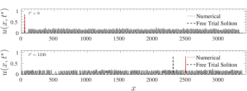
Figure 2: (adapted from Carbone et al. (2016)) Comparison for the propagation of a free soliton with the spectral parameter $\eta=\eta_{1}$ in a void (black dashed line) with the propagation of the trial soliton with the same spectral parameter $\eta_{1}$ (red solid line) through a rarefied soliton gas with the DOS supported on a narrow spectral interval around $\eta_{0}<\eta_{1}$. One can see that the trial soliton propagates faster in the gas due to the interactions with smaller solitons. Reproduced with permission.

For a weakly non-homogeneous (out of equilibrium) gas we have $f(\eta)\rightarrow f(\eta;x,t)$, $s(\eta)\rightarrow s(\eta;x,t)$, where the $(x,t)$-variations of $f$ and $s$ occur on macroscopic, Euler, scales, much larger than the typical scales associated with variations of the wave field $u(x,t)$ in individual solitons.

Now, isospectrality of the KdV evolution within the IST framework implies the continuity equation for the phase space density (the DOS),

$$\partial_{t}f+\partial_{x}(sf)=0,$$ (13)

which, together with (12), provides the spectral hydrodynamic/kinetic description of a rarefied KdV soliton gas.

II.3 Dense soliton gas

If the KdV soliton gas is sufficiently dense, the simple heuristic construction of the previous section based on the assumption of short-range interactions between solitons becomes, strictly speaking, invalid as solitons in such a gas strongly overlap and hence, are involved in a continual nonlinear interaction so that the corresponding KdV solution can nowhere be represented as a linear superposition of individual solitons as in (9), cf. Fig. 3 (b). In particular, the approximation (11) for the total phase shift based on the free soliton velocities ceases to be valid.

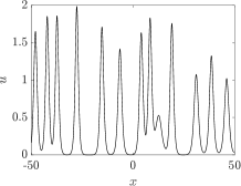
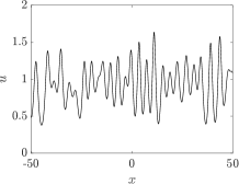
Figure 3: Rarefied (left) vs dense (right) KdV soliton gases with the same spectral density $\phi(\eta)=\eta/{\sqrt{1-\eta^{2}}}$ but different spatial densities: $\alpha\simeq 0.1$ (left) and $\alpha\simeq 0.3$ (right).

A general (dense or rarefied) KdV soliton gas at equilibrium can be defined as a non-decaying random solution of the KdV equation whose realizations can be approximated, on any sufficiently large interval $[x_{0}-L/2,x_{0}+L/2]$, by an appropriate $N$-soliton solution with $N\sim L\gg 1$ so that: (i) the gas has finite spatial density $\alpha$ following the thermodynamic limit ($L,N\to\infty$, $N/L\to\alpha$); (ii) the soliton spectral parameters $\eta_{i}$, $j=1,2,\dots,N$, are distributed on some finite interval $\Gamma\in\mathbb{R}^{+}$ with density $\phi(\eta)>0$ defined for $N\to\infty$ via

$$\eta_{j+1}-\eta_{j}\sim\frac{1}{\phi(\eta_{j})N},\quad\int_{\Gamma}\phi(\eta)\mathrm{d}\eta=1,$$ (14)

so that $\phi(\eta)$ does not depend on the chosen realization of soliton gas and on the reference point $x_{0}$. The set of discrete spectral parameters $\{\eta_{i}\}$ in $N$-soliton solutions is complemented by the associated set of norming constants, whose phases can be interpreted for diluted gases in terms of the spatial locations of individual solitons within the $N$-soliton solution, see Drazin and Johnson (1989); Novikov et al. (1984); Ablowitz et al. (1974). Randomness enters this soliton gas construction in two ways: (i) spectral—via interpreting $\phi(\eta)\mathrm{d}\eta$ as a probability measure on $\Gamma$; (ii) spatial—by assuming that the phases of the norming constants are random values uniformly distributed on some fixed interval. The above definition of soliton gas as the thermodynamic limit of $N$-soliton solutions, while lacking full mathematical rigour, is physically intuitive and sufficient for the majority of practical (numerical or experimental) considerations, where one inevitably deals with finite numbers of solitons. It can also be readily generalized to other integrable equations (see Section IV for the implementation of this construction in the context of the fNLS equation).

II.3.1 Density of states

The phenomenological definition of the DOS $f(\eta)$ introduced in Section II.2 for rarefied soliton gas can be meaningfully interpreted in the context of a dense gas where solitons strongly interact and cannot be identified as individual localized wave structures. Consider a typical realization of a uniform soliton gas at some $t=t^{*}$ for $x\in[x_{0}-L/2,x_{0}+L/2]$, $L\gg 1$. We now impose zero boundary conditions for $x\notin[x_{0}-L/2,x_{0}+L/2]$, and consider $U_{L}(x)=\chi_{{[x_{0}-L/2,x_{0}+L/2]}}u(x,t^{*})$, where $\chi_{[a,b]}$ is the indicator function. Replacing $U_{L}$ by the approximating $N$-soliton solution $u_{N}$ with $N\gg 1$ one determines the density $\phi(\eta)$ of the discrete spectrum points $\eta_{j}\in\Gamma$, $j=1,\dots,N$ (14) and the spatial density of the gas $\alpha\sim N/L$. One simple way to realize this construction practically is to use $U_{L}(x)$ as the initial condition for KdV and evolve it in time, see Fig. 4. One then infers $\phi(\eta)$, $\Gamma$ and $\alpha$ from the analysis of the distribution of soliton amplitudes $a_{i}=2\eta_{i}^{2}$ in the resulting soliton train at sufficiently large $t$.

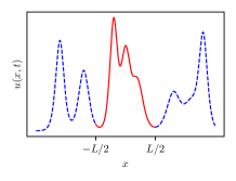
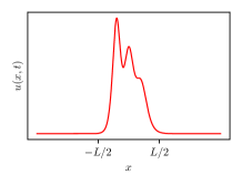
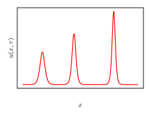
Figure 4: Schematic illustrating the $N$-soliton approximation of the ‘windowed’ portion $U_{L}(x)$ of a KdV soliton gas at some $t=t^{*}$ (upper row) and its evolution into the ordered soliton train at $t=\tau\gg t^{*}$ (lower plot).

We introduce the partial DOS $f_{L}(\eta)=\varkappa\phi(\eta)$, where the coefficient $\varkappa$ is determined from the normalization $\int_{x_{0}-L/2}^{x_{0}+L/2}\int_{\Gamma}f_{L}(\eta)\mathrm{d}\eta\mathrm{d}x=N$, consistent with the DOS definition in Section II.2. Then the limit $\lim\limits_{L\to\infty}f_{L}(\eta)\equiv f_{\rm eff}(\eta)$ can be viewed as the effective DOS of a dense soliton gas. Using (10) and (14) we find the normalization constant $\varkappa=\alpha$ so that

$$f_{\rm eff}(\eta)=\alpha\phi(\eta)\,.$$ (15)

Shown in Fig 3 are realizations of two soliton gases with the same $\phi(\eta)$ and different $\alpha$’s. We note that the criterion $\alpha\ll 1$ for rarefied gas is understood in the formal, asymptotic sense since the actual, numerical, value of $\alpha$ depends on the definition of the (mesoscopic) unit interval of $x$.

As we shall see in Section III, in a more general soliton gas setting based on finite-gap theory one has $\varkappa\equiv\varkappa(\eta)$, which is interpreted as the ‘scaled spectral wavenumber’ responsible for the spatial density of solitons with a given spectral parameter. However, the above phenomenological setting with $\varkappa$ constant is a useful approximation that is particularly relevant to the numerical realization of soliton gases (see Gelash et al. (2019); Congy et al. (2022) and Section IV) and identifying their connection with GHD (see T et al. (2022) and Section VII).

II.3.2 Kinetic equation

For a weakly non-uniform gas we assume scale separation, where the gas is considered to be at local equilibrium over intermediate, mesoscopic, scale involving sufficiently large numbers of solitons, while appreciable $(x,t)$-variations of the DOS occur on a larger, macroscopic, Euler, scale. We note that this scale separation is at heart of GHD, where the mesoscopic scale is associated with the notion of ‘fluid cells’, where the entropy is locally maximized with respect to the infinite number of conserved quantities Castro-Alvaredo et al. (2016); Doyon (2020), see Section VII.

The generalization of Zakharov’s kinetic equation to the case of a dense gas was derived in El (2003) (see Section III.2 below). It involves the same continuity equation (13) for the DOS but the approximate expression (12) for the tracer velocity is replaced by the exact integral equation of state:

$$s(\eta)=4\eta^{2}+\frac{1}{\eta}\int_{\Gamma}\ln\left|\frac{\eta+\mu}{\eta-\mu}\right|f(\mu)[s(\eta)-s(\mu)]\mathrm{d}\mu\,,$$ (16)

where we have dropped for brevity the $(x,t)$-dependence for $f(\eta)$ and $s(\eta)$.

In simple terms (16) represents an extrapolation of the rarefied gas properties to a dense gas, realised by replacing $s_{0}(\eta)\to s(\eta)$ in the collision rate expression (11). This observation has led in El and Kamchatnov (2005) to the phenomenological prescription for the construction of the soliton gas equation of state involving the free soliton velocity $s_{0}(\eta)$ and the phase shift expression $\Delta(\eta,\mu)=\mathrm{sgn}[(s_{0}(\eta)-s_{0}(\mu)]G(\eta,\mu)$, specific to each integrable system:

$$s(\eta)=s_{0}(\eta)+\int_{\Gamma}G(\eta,\mu)f(\mu)[s(\eta)-s(\mu)]\mathrm{d}\mu\,.$$ (17)

In the fNLS case, the solitonic spectrum $\{\lambda_{j}\}$ in the associated linear (Zakharov-Shabat) scattering problem is complex (see Section IV.1 below) so that the DOS $f(\lambda)$ is generally supported on some compact Schwarz symmetric 2D set $\Lambda\subset\mathbb{C}$ so it is sufficient to consider only the upper half plane part $\Lambda^{+}$ (here Schwarz symmetry means that if $\lambda\in\mathbb{C}$ is a point of the spectrum then so is the c.c. point $\lambda^{*}$). Then, using $s_{0}(\lambda)=-4\hbox{Re}\lambda$ for the free-soliton velocity and the expression (8) for the two-soliton scattering shift, the kinetic equation for the fNLS soliton gas assumes the form El and Kamchatnov (2005)

$$\begin{split}&f_{t}+(fs)_{x}=0,\\ &s(\lambda;x,t)=-4\hbox{Re}\lambda+\\ &\frac{1}{\hbox{Im}\lambda}\iint\limits_{\Lambda^{+}}\ln\left|\frac{\mu-\lambda^{*}}{\mu-\lambda}\right|[s(\lambda;x,t)-s(\mu;x,t)]f(\mu;x,t)\mathrm{d}\xi\mathrm{d}\zeta,\end{split}$$ (18)

where $\mu=\xi+i\zeta$ and $\Lambda^{+}\subset\mathbb{C}^{+}\setminus i\mathbb{R}^{+}$.

The special case when all discrete spectrum points are located on the imaginary axis, $\Lambda^{+}\subset i\mathbb{R}^{+}$, corresponds to non-propagating multisoliton solutions called bound states Zakharov and Shabat (1972). This case requires a separate consideration. since for the corresponding bound state soliton gas $\hbox{Re}\lambda=0$ the equation of state in (18) immediately yields $s(\lambda)=0$ resulting in the equilibrium DOS, $f_{t}=0$.

II.3.3 Conserved quantities

One of the fundamental properties of integrable dynamics is the availability of an infinite set of conservation laws

$$\partial_{t}P_{n}+\partial_{x}Q_{n}=0,\quad n=1,2,\dots\;,$$ (19)

where the $P_{n}$ and $Q_{n}$ are functions of the field variable $u$ and its derivatives. For the KdV equation, of particular interest are the first three conserved densities:

$$P_{1}=u,\quad P_{2}=u^{2},\quad P_{3}=\frac{u_{x}^{2}}{2}-u^{3}\,,$$ (20)

typically associated with the “mass”, “momentum” and “energy” conservation. Their counterparts for the fNLS equation (equation (10) with $\sigma=+1$) have the form Zakharov and Shabat (1972)

$$P_{1}={|\psi|^{2}},\ \ P_{2}=\text{Im}(\psi_{x}\psi^{*}),\ \ P_{3}=|\psi|^{4}-|\psi_{x}|^{2}.$$ (21)

For non-equilibrium soliton gas dynamics conservation equations (19) are replaced by their averaged analogs:

$$\partial_{t}\langle P_{n}[u]\rangle+\partial_{x}\langle Q_{n}[u]\rangle=0,\quad n=1,2,\dots,$$ (22)

where $\langle\cdot\rangle$ denotes ensemble averaging, and the $x,t$-variations in (19) occur on much larger scales than in (19).

In contrast with the discrete set of conservation laws (19) for the original equation, kinetic equation (13) possesses a continuum of conserved quantities. Indeed, (13) implies that for any $h(\eta)\neq 0$, $\int_{\Gamma}h(\eta)f(\eta;x,t)\mathrm{d}\eta$ is a density of the conserved quantity with $\int_{\Gamma}h(\eta)f(\eta;x,t)s(\eta;x,t)\mathrm{d}\eta$ being the corresponding flux density. For the KdV equation, the densities of the special “Kruskal” series (22) are given by El (2003, 2016)

$$\langle P_{n}[u]\rangle=C_{n}\int_{\Gamma}\eta^{2n-1}f(\eta)\mathrm{d}\eta,,\ \ n=1,2,\dots,$$ (23)

where the coefficients $C_{n}$ depend on the normalization of the conserved densities. For the physical densities (20) we have

$$C_{1}=4,\quad C_{2}={16}/{3},\quad C_{3}={32}/{5}.$$ (24)

Expressions (23), (24) are readily obtained by considering a large portion of a homogeneous soliton gas: $u_{L}=\chi_{[0,L]}u(x,t)$ with $L\gg\alpha^{-1}$ at some arbitrary $t=t^{*}$. Assuming ergodicity one can replace the ensemble average $\langle P_{n}\rangle$ by the spatial average $L^{-1}\int_{x_{0}}^{x_{0}+L}P_{n}[u_{L}]\mathrm{d}x$ which is a conserved quantity and can be evaluated over the long-time asymptotic solution: $u_{L}\sim\sum_{i}u_{s}(x,t;\eta_{i})$ as $t\to\infty$.

A fundamental restriction imposed on the DOS $f(\eta)$ follows from non-negativity of the variance $\mathcal{A}\ =\ \sqrt{\langle{u^{2}}\rangle\ -\ \langle{u}\rangle^{2}}\ \geqslant\ 0,$ or equivalently, recalling (23), (24)

$$\int_{\Gamma}\eta^{3}f(\eta)\,\mathrm{d}\eta-3\left(\int_{\Gamma}\eta f(\eta)\,\mathrm{d}\eta\right)^{2}\geqslant\ 0\;.$$ (25)

For the fNLS equation the averaged conserved densities can also be expressed in terms of moments of the DOS as Tovbis and Wang (2022)

$$\langle P_{n}[\psi]\rangle=C_{n}\iint\limits_{\Lambda^{+}}{\rm Im}(\lambda^{n})f(\lambda)\mathrm{d}\xi\mathrm{d}\zeta,\quad n=1,2,\dots$$ (26)

where $\lambda=\xi+i\zeta$ and the coefficients $C_{n}$ for the physical conserved quantities (21) are

$$C_{1}=4,\quad C_{2}=-4,\quad C_{3}={16}/{3}.$$ (27)

III Spectral theory of soliton gas

III.1 General framework

The phenomenological kinetic theory of soliton gas described in the previous section is essentially based on the interpretation of solitons as quasi-particles experiencing short-range pairwise interactions accompanied by the well-defined phase/position shifts. As was already stressed, although this theoretical framework is justifiable in the case of rarefied gas, it is less satisfactory for a dense gas where solitons experience significant overlap and continual nonlinear interactions so that they could become indistinguishable as separate entities. This suggests that a more consistent theoretical approach involving the wave aspect of the soliton’s “dual identity” is necessary. In this section we outline a general mathematical framework for the spectral theory of soliton gas based on the thermodynamic limit of nonlinear multiphase solutions of integrable equations. This approach has been first developed in El (2003) for KdV equation and more recently applied to the description of fNLS soliton and breather gases El and Tovbis (2020).

With the KdV equation as the simplest prototypical example in mind we consider the family of multiphase solutions of the form

$$u(x,t)=F_{N}(\theta_{1},\dots,\theta_{N}),\quad\theta_{j}=k_{j}x-\omega_{j}t+\theta_{j}^{0},$$ (28)

where $k_{j}$ and $\omega_{j}$, $j=1,\dots,N$ are the wavenumbers and frequencies (generally incommensurable), and the function $F_{N}$ is $2\pi$-periodic with respect to each phase component $\theta_{j}\in[-\pi,\pi)$, $\theta_{j}^{0}$ being initial phases. (In the context of the NLS equation (6) the representation (28) is valid for $|\psi|$). We stress that the existence of multiphase quasiperiodic solutions (28) to a nonlinear dispersive equation is a unique property of integrable systems. Such solutions are typically expressed in terms of Riemann theta-functions, see e.g. Osborne (2010) but we won’t be using their specific form here.

It has been discovered in 1970-s that multiphase solutions to integrable equations have remarkable spectral properties defined within the (quasi-)periodic analogue of IST called the finite-gap theory, see Novikov et al. (1984); Osborne (2010). The fundamental result of the finite gap theory is that the IST spectrum $\mathcal{S}_{N}$ of the $N$-phase solution (28) lies in the union of $N+1$ disjoint bands $\gamma_{j}=[\lambda_{2j-1},\lambda_{2j}]$, $j=1,\dots,N+1$,

$$\lambda\in\mathcal{S}_{N}\equiv\cup_{i=1}^{N+1}\gamma_{i},\quad\gamma_{i}\cap\gamma_{j}=\emptyset,\ \ i\neq j$$ (29)

separated by $N$ finite gaps $c_{j}=(\lambda_{2j},\lambda_{2j+1})$. The number of spectral gaps $N$ is called the genus.

For the preliminary discussion of this section it is convenient to assume that the spectrum $\mathcal{S}_{N}$ is real-valued. This is the case for the (unidirectional) KdV equation and (bidirectional) defocusing NLS equation (equation (6) with $\sigma=-1$). The case of complex band spectrum, $\mathcal{S}_{N}\subset\mathbb{C}$, arises for the fNLS equation, and this case will be considered separately in Section III.3. We also note that one of the spectral bands could be semi-infinite (as is the case for the KdV equation), then $\gamma_{N+1}=[\lambda_{2N+1},+\infty)$. Thus the spectrum of a finite-gap solution (also called finite-gap potential) is fully parametrised by the state vector ${\bm{\lambda}}={(\lambda_{1},\lambda_{2},\dots,\lambda_{\mathcal{D}})}$, where $\mathcal{D}=2N+1$ or $\mathcal{D}=2N+2$ depending on the presence or absence of the semi-infinite band.

One of the important outcomes of the finite-gap theory are the nonlinear dispersion relations (NDRs) linking the physical parameters of the multiphase solution (28) such as the wavenumbers, the frequencies and the mean with the components of the $\mathcal{D}$-dimensional spectral state vector ${\bm{\lambda}}$. In particular, for the $N$-component wavenumber and frequency vectors ${\bm{k}}=(k_{1},\dots,k_{N})$ and ${\bm{\omega}}=(\omega_{1},\dots,\omega_{N})$ in (28) the NDRs can be represented as

$$k_{j}={K}_{j}({\bm{\lambda}}),\qquad\omega_{j}=\Omega_{j}({\bm{\lambda}}),\quad j=1,\dots,N,$$ (30)

where ${K}_{j}({\bm{\lambda}}),\ \Omega_{j}({\bm{\lambda}})$ are typically expressed in terms of complete hyperelliptic integrals, see e.g. Osborne (2010); Flaschka et al. (1980); El and Tovbis (2020).

By manipulating the endpoints of spectral bands $\lambda_{j}$ one can modify the waveform of the solution (28). In particular, by collapsing all spectral bands into double points, $\lambda_{2j-1},\lambda_{2j}\to\lambda^{j}_{*}$, $j=1,\dots,N$, the $N$-gap solution transforms into $N$-soliton solution with the discrete spectrum eigenvalues $\lambda_{*}^{j}$ Novikov et al. (1984) (for the KdV equation $\lambda_{*}^{j}=-\eta_{j}^{2}$, see Section II.1). This solitonic transition corresponds to the limit $k_{j},\omega_{j}\to 0,(\omega_{j}/k_{j})\to s_{0}(\lambda_{*}^{j})=\mathcal{O}(1)$, where $s_{0}(\lambda)$ is the velocity of a free soliton corresponding to the discrete spectral eigenvalue $\lambda_{*}^{j}$. (We note that any linear combination of wavenumbers with integer coefficients is also a wavenumber, so by $\{k_{j}\}_{j=1}^{N}$ we always assume a particular, “fundamental”, set of the wavenumbers that vanish in the solitonic limit). Thus, finite-gap potentials represent periodic or quasiperiodic generalizations of multisoliton solutions. Importantly, finite-gap potentials, unlike $N$-soliton solutions, are non-decaying functions with nonzero mean, which makes them natural building blocks for the construction of equilibrium, spatially uniform, soliton gases. Another advantage of using finite-gap solutions for the soliton gas construction is the presence of a natural probability measure—the uniform measure on the $N$-dimensional phase torus $\mathbb{T}^{N}$ of (28), i.e. each phase $\theta_{j}^{0}\in[-\pi,\pi)$ is assumed to be a random value uniformly distributed on the period. Assuming incommensurability of the wavenumbers $k_{j}$ and frequencies $\omega_{j}$ this measure gives rise to the ergodic random process with realizations defined by (28).

The dynamics of weakly non-uniform finite-gap potentials are described by the Whitham modulation theory Whitham (1999); Kamchatnov (2000); Flaschka et al. (1980), which prescribes slow evolution of the spectrum, $\lambda_{j}(x,t)$, on the spatiotemporal scales much larger than those associated with ‘rapid’ variations of the wave (28) itself. The modulation system inherently includes wave conservation equations

$$\partial_{t}k_{j}+\partial_{x}\omega_{j}=0,\quad j=1,\dots,N,$$ (31)

where $k_{j}({\bm{\lambda}})$ and $\omega_{j}({\bm{\lambda}})$ are given by the NDRs (30).

We now define equilibrium soliton gas via the thermodynamic limit of finite-gap potentials El and Tovbis (2020). Namely, we consider a sequence of finite-gap potentials (28) such that

$$\quad N\to\infty:\ \ k_{1},\dots,k_{N}\to 0,\ \ \sum\limits_{j=1}^{N}k_{j}\to 2\pi\alpha=\mathcal{O}(1),$$ (32)

with a similar behaviour for the frequency components $\omega_{j}$ so that $\omega_{j}/k_{j}=\mathcal{O}(1)$. The limit (32) suggests the following asymptotic scaling for the fundamental wavenumbers and frequencies as $N\to\infty$:

$$N\to\infty:\quad k_{j}\sim\omega_{j}\sim N^{-1}.$$ (33)

It can be shown quite generally that under the limit (32) the uniform distribution for the initial phases $\theta_{j}^{0}\in[-\pi,\pi)$, $j=1,\dots,N$ transforms to the Poisson distribution with the density parameter $\alpha$ on $\mathbb{R}$ for the ‘position phases’ $l_{j}^{0}\equiv\theta_{j}^{0}/k_{j}$ El (2021). We associate the limiting random process $\lim_{N\to\infty}F_{N}({\bm{\theta}})$ satisfying (32) with soliton gas. By construction this process is ergodic. As we shall see, the above definition is consistent with the phenomenological construction of soliton gas in Section II.3.

As we show in the next section, the thermodynamic limit (32) is achieved by imposing a special band-gap distribution (scaling) for the spectrum $\mathcal{S}_{N}$ for $N\gg 1$. Generally the spectral bands are required to be exponentially narrow compared to the gaps although the super-exponential and sub-exponential scalings are also possible and these corresponds to the noninteracting (ideal) soliton gas and soliton condensate respectively. In all cases we shall call the corresponding limit as $N\to\infty$ of a function $F({\bm{\lambda}})$ defined on $\mathcal{S}_{N}$ the thermodynamic limit of $G$.

The density of states $f(\lambda)$ is then defined via the thermodynamic limit of the partial sum

$$\frac{1}{2\pi}\sum\limits_{j=1}^{M\leq N}k_{j}\to\int\limits_{\lambda_{\min}}^{\lambda}f(\lambda^{\prime})\mathrm{d}\lambda^{\prime},$$ (34)

where $\lambda$ is a continuous spectral variable interpolating the discrete positions $\lambda_{j}^{*}$ of the band centres; as a matter of fact $\int_{\lambda_{\min}}^{\lambda_{\max}}f(\lambda^{\prime})\mathrm{d}\lambda^{\prime}=\alpha$, cf. (10).

Similarly, we have

$$\frac{1}{2\pi}\sum\limits_{j=1}^{M\leq N}\omega_{j}\to\int\limits_{\lambda_{\min}}^{\lambda}v(\lambda^{\prime})\mathrm{d}\lambda^{\prime},$$ (35)

where $v(\lambda)$ is the spectral flux density; then $s(\lambda)=v(\lambda)/f(\lambda)$ has the meaning of the soliton gas transport velocity that can also be interpreted as an average tracer soliton velocity in the gas.

Applying the thermodynamic limit (34), (35) to the NDRs (30) for finite-gap solutions one obtains the NDRs for an equilibrium soliton gas and hence, the equation of state $s(\lambda)=\mathcal{F}[f(\lambda)]$, which typically has the form of a linear integral equation (17). Further, assuming $f\equiv f(\lambda;x,t)$, $s\equiv s(\lambda;x,t)$ and applying the thermodynamic limit to the modulation equations (31), we obtain the continuity equation (13) for DOS in a non-equilibrium gas.

III.2 Korteweg-de Vries equation

We now present the results of the application of the above general spectral construction to the KdV equation (1) following Refs. El (2003, 2021) The key input ingredient of the theory are the discrete NDRs (30) for finite-gap potentials. The specific expressions for the KdV NDRs can be found elsewhere (see e.g. Flaschka et al. (1980); El (2003, 2021)), here we only discuss their thermodynamic limit as $N\to\infty$.

First we recall that the $N$-soliton limit of an $N$-gap solution is achieved by collapsing all the finite bands $\gamma_{j}$ in the spectral set $\mathcal{S}_{N}$ (29) into double points corresponding to the soliton discrete spectral values. It was proposed in El (2003) that the special infinite-soliton limit of the spectral $N$-gap KdV solutions, termed the thermodynamic limit, provides spectral description the KdV soliton gas. The thermodynamic limit is achieved by assuming a special band-gap distribution (scaling) of the spectral set $\mathcal{S}_{N}$ for $N\gg 1$ on the fixed interval $[\lambda_{1},\lambda_{2N+1}]$ (e.g. $[-1,0]$). Specifically, we require the spectral bands $\gamma_{j}$ to be exponentially narrow compared to the gaps $c_{j}$ so that for $N\to\infty$ the spectral set $\mathcal{S}_{N}$ is asymptotically characterized by two continuous positive functions: the density $\phi(\eta)$ of the lattice points $\eta_{j}\in\Gamma\subset\mathbb{R}^{+}$ defining the band centers via $-\eta_{j}^{2}=(\lambda_{2j}+\lambda_{2j-1})/2$, and the logarithmic bandwidth distribution $\tau(\eta)$ defined for $N\to\infty$ by

$$\eta_{j}-\eta_{j+1}\sim\frac{1}{N\phi(\eta_{j})},\quad\tau(\eta_{j})\sim-\frac{1}{N}\ln(\lambda_{2j}-\lambda_{2j-1}).$$ (36)

Additionally, invoking the asymptotic behaviors (33) we introduce the interpolating functions $\kappa(\eta)$, $\nu(\eta)$ for the scaled wavenumbers and frequencies

$$k_{j}\sim\frac{\kappa(\eta_{j})}{N},\quad\omega_{j}\sim\frac{\nu(\eta_{j})}{N}.$$ (37)

Then the definitions (34) and (35) of the DOS and the spectral flux density imply

$$f(\eta)=\frac{1}{2\pi}\kappa(\eta)\phi(\eta),\quad v(\eta)=\frac{1}{2\pi}\nu(\eta)\phi(\eta),$$ (38)

where we have used a more convenient in the KdV context spectral variable $\eta$ instead of $\lambda=-\eta^{2}$. Now, considering the KdV finite-gap NDRs (30) subject to the thermodynamic scaling (36) , (37) and letting $N\to\infty$, yields the integral equations El (2003, 2021):

$$\begin{split}&\int_{\Gamma}\ln\left|\frac{\mu+\eta}{\mu-\eta}\right|f(\mu)\mathrm{d}\mu+f(\eta)\sigma(\eta)=\eta,\\ &\int_{\Gamma}\ln\left|\frac{\mu+\eta}{\mu-\eta}\right|v(\mu)\mathrm{d}\mu+v(\eta)\sigma(\eta)=4\eta^{3}\end{split}$$ (39)

for all $\eta\in\Gamma$ (if $\Gamma$ is a fixed, simply-connected compact interval one can set $\Gamma=[0,1]$ without loss of generality). Here the spectral scaling function $\sigma:\Gamma\to[0,\infty)$ is a continuous non-negative function that encodes the Lax spectrum of the soliton gas via $\sigma(\eta)=\tau(\eta)/\phi(\eta)$. Equations (39) are the KdV soliton gas NDRs.

Eliminating $\sigma(\eta)>0$ from the NDRs (39) yields the equation of state (16) for the KdV soliton gas. Next, for a non-homogeneous soliton gas $f(\eta)\equiv f(\eta;x,t)$, $v(\eta)\equiv v(\eta;x,t)$, and the application of the thermodynamic limit to the modulation equations (31) yields the continuity equation (13) for the DOS. Indeed, (31) imply

$$\left(\frac{1}{2\pi}\sum\limits_{j=1}^{M\leq N}k_{j}\right)_{t}+\left(\frac{1}{2\pi}\sum\limits_{j=1}^{M\leq N}\omega_{j}\right)_{x}=0.$$ (40)

for $M=1,\dots,N$. Applying the thermodynamic limit (34), (35) to (40) we obtain the kinetic equation $f_{t}+(fs)_{x}=0$ as required.

Thus, the spectral kinetic equation (13), (16) for soliton gas represents the thermodynamic limit of the KdV-Whitham modulation system El (2003). We note that condition $\sigma>0$ used in the derivation of the equation of state (16) implies the restriction $\eta^{-1}\int_{\Gamma}\ln\left|\frac{\mu+\eta}{\mu-\eta}\right|f(\mu)\mathrm{d}\mu<1$ on the admissible DOS $f(\eta)$, complementing the earlier formulated restriction (25). The limiting case $\sigma=0$ corresponds to the special soliton gas termed soliton condensate, see Section III.4 below.

III.3 Focusing nonlinear Schrödinger equation

The spectral theory of soliton gas for the fNLS equation was developed in El and Tovbis (2020). It follows the same general framework of the thermodynamic limit of finite-gap potentials outlined in Section III.1 resulting in the kinetic equation (18) for the dense gas of fundamental fNLS solitons. However, due to the fact that the finite-gap spectral set for the fNLS equation lies in the complex plane, $\lambda\in\mathbb{C}$, the spectral theory of fNLS soliton gas admits a much broader range of scenarios than the KdV theory. In particular, it covers the case of breather gases, including infinite random ensembles of interacting Akhmediev, Kuznetsov-Ma and Peregrine breathers Roberti et al. (2021). Another highly nontrivial object is the gas of bound state fNLS solitons (bound states are $N$-soliton solutions with all discrete spectral parameters $\lambda_{j}$, $j=1,\dots,N$ having the same, possibly zero, real part Zakharov and Shabat (1972)). The latter was shown in Gelash et al. (2019) to represent an accurate model for the nonlinear stage of the development of spontaneous (noise induced) modulation instability, see Section VI.2.

The soliton gas theory for the fNLS equation is more technically involved than in the KdV case. Here we only present the NDRs for the fNLS soliton gas, a counterpart of the KdV NDRs (39):

$$\begin{split}&\int_{\Gamma^{+}}\ln\left|\frac{\mu-\bar{\lambda}}{\mu-\lambda}\right|f(\mu)|\mathrm{d}\mu|+\sigma(\lambda)f(\lambda)=\text{Im}\lambda,\\ &\int_{\Gamma^{+}}\ln\left|\frac{\mu-\bar{\lambda}}{\mu-\lambda}\right|v(\mu)|\mathrm{d}\mu|+\sigma(\lambda)v(\lambda)=-4\text{Im}\lambda\,\text{Re}\lambda,\end{split}$$ (41)

where $\Gamma^{+}$ is the upper part of the 1D Schwarz-symmetric curve $\Gamma\subset\mathbb{C}$ — the spectral support of the DOS $f(\lambda)$ (in the general 2D case the integration with respect to arc length of $\Gamma^{+}$ in (41) is replaced by the integration over a 2D compact domain $\Lambda^{+}\subset\mathbb{C}^{+}$: $\int\limits_{\Gamma^{+}}\dots|\mathrm{d}\mu|\to\iint\limits_{\Lambda^{+}}\dots\mathrm{d}\xi\mathrm{d}\zeta\,$, where $\mu=\xi+i\zeta$).

Eliminating the spectral scaling function $\sigma(\lambda)$ from the NDRs (41) we obtain the equation of state in the kinetic equation (18). The continuity equation in (18) is derived via the thermodynamic limit of the modulation equations (31), similar to the KdV case. See Ref. El and Tovbis (2020) for details.

Concluding this Section, we note that the requirement for the spectral support $\Gamma^{+}$ (or $\Lambda^{+}$) to be a compact set is purely technical and can be dropped so that the integrals in the NDRs and the equation of state can be taken over semi-infinite spectral domains: the only important requirement is the sufficiently fast decay of the DOS ensuring the existence of the integrals. The same is true for the KdV SG equations.

III.4 Polychromatic soliton gases and soliton condensates

Integration of the spectral kinetic equation (13), (17) for soliton gas in any generality represents a challenging mathematical problem. One can, however, consider some physically interesting particular cases that admit effective analytical treatment. The most obvious one is the case of spectrally polychromatic gases studied in El et al. (2011). The DOS of a polychromatic soliton gas represents a linear combination of the ‘monochromatic’ components in the form of Dirac delta-functions centered at distinct spectral points $\zeta_{j}\in\Gamma$ (note that $\Gamma$ can be real or complex domain, depending on the original dispersive equation)

$$f(\lambda;x,t)=\sum\limits_{j=1}^{M}w_{j}(x,t)\delta(\lambda-\zeta_{j}),$$ (42)

where $w_{j}(x,t)>0$ are the components’ weights, and $\{\zeta_{j}\}_{j=1}^{M}\subset\Gamma$, $(\zeta_{j}\neq\zeta_{k}\iff j\neq k)$. Substitution of (42) into the kinetic equation (13), (17) reduces it to a system of hyperbolic hydrodynamic conservation laws

$$(w_{i})_{t}+(w_{i}s_{i})_{x}=0,\qquad i=1,\dots,M\,,$$ (43)

where the component densities $w_{i}(x,t)$ and the transport velocities $s_{j}(x,t)\equiv s(\zeta_{j},x,t)$ are related algebraically:

$$s_{j}=s_{0j}+\sum\limits_{m=1,m\neq j}^{M}G_{jm}w_{m}(s_{j}-s_{m}),\quad j=1,2,\dots M.$$ (44)

Here we used the notation $s_{0j}\equiv s_{0}(\zeta_{j}),\quad G_{jm}\equiv G(\zeta_{j},\zeta_{m}),\quad j\neq m$. One should also mention an important restriction $\sum\limits_{m=1,m\neq j}^{M}G_{jm}w_{m}<1$ equivalent to the condition of positivity of the spectral scaling function $\sigma$ in the thermodynamic limit construction.

We note that the delta-function representation (42) is a mathematical idealisation, which has a formal sense in the context of the integral equation of state (17), but cannot be applied to the original dispersion relations where it appears in both the integral and the secular terms (cf. (39) for the KdV equation). In a physically realistic description the delta-functions in (42) should be replaced by some narrow distributions around the spectral points $\zeta_{j}$, i.e. we first take the thermodynamic limit $N\to\infty$ and then allow the distributions to become sharply peaked.

For $M=2$ system (44) can be solved to give explicit expressions for $s_{1,2}(w_{1},w_{2})$:

$$\begin{split}s_{1}=s_{01}+\frac{G_{12}w_{2}(s_{01}-s_{02})}{1-(G_{12}w_{2}+G_{21}w_{1})},\\ s_{2}=s_{02}-\frac{G_{21}w_{1}(s_{01}-s_{02})}{1-(G_{12}w_{2}+G_{21}w_{1})}.\end{split}$$ (45)

As was shown in El and Kamchatnov (2005) (see also Kamchatnov and Shaykin (2022)) the two-component system (43), (45) is equivalent to the so-called Chaplygin gas equations that occur in certain theories of cosmology (see e.g. Bento et al. (2002)), and to the Born-Infeld equations arising in nonlinear electromagnetic field theory Born and Infeld (1934), Whitham (1999).

It was shown in El et al. (2011) that the system (43), (44) for any $M\in\mathbb{N}$ possesses $M$ Riemann invariants and belongs to the special class of linearly degenerate, semi-Hamiltonian systems of hydrodynamic type Ferapontov (1991). Linear degeneracy of (43), (44) implies the absence of the wavebreaking and shock formation for generic initial-value problems with smooth Cauchy data Rozhdestvenskii and Janenko (1983). On the other hand, it implies that the solution to a Riemann (the evolution of an initial discontinuity) problem for polychromatic soliton gas will be given by a combination of differing constant states $w_{i}=const_{j}$, separated by contact discontinuities propagating with classical shock speeds found from the Rankine-Hugoniot conditions for the conservation laws (43),(44). Such weak solutions were constructed in Refs. El and Kamchatnov (2005); Carbone et al. (2016); Congy et al. (2021); El (2021) for various soliton gases. More general solutions are available via the hodograph transform, see El et al. (2011); Kamchatnov and Shaykin (2022).

Another special class of soliton gases is presented by soliton condensates whose properties are dominated by the collective effect of soliton interactions while the individual soliton dynamics are completely suppressed. Soliton condensates were first introduced in El and Tovbis (2020) for the fNLS equation and then thoroughly studied in Congy et al. (2022) for the KdV equation. Spectrally, a soliton condensate is realized by vanishing the spectral scaling function, $\sigma(\eta)\to 0$, in the soliton gas NDRs (equations (39) for KdV or (41) for fNLS). For the KdV case the condensate NDRs are then given by Congy et al. (2022)

$$\int_{\Gamma}\ln\left|\frac{\mu+\eta}{\mu-\eta}\right|f(\mu)d\mu=\eta,\quad\int_{\Gamma}\ln\left|\frac{\mu+\eta}{\mu-\eta}\right|v(\mu)d\mu=4\eta^{3}.$$ (46)

For the simplest case $\Gamma=[0,q]$ these are solved by

$$f(\eta)=\frac{\eta}{\pi\sqrt{q^{2}-\eta^{2}}},\quad v(\eta)=\frac{6\eta(2\eta^{2}-1)}{\pi\sqrt{q^{2}-\eta^{2}}}.$$ (47)

The counterpart fNLS solution of the NDRs (41) with $\lambda\in\Gamma^{+}=[0,iq]$ and $\sigma=0$ is given by El and Tovbis (2020)

$$f(\lambda)=\frac{-i\lambda}{\pi\sqrt{q^{2}+\lambda^{2}}},\quad v(\lambda)=0\,,$$ (48)

—and describes the DOS $f(\lambda)$ in the non-propagating, bound state ($s=v/f=0$) soliton condensate. By choosing a different 1D support $\Gamma^{+}\subset\mathbb{C}^{+}$ one can construct other types of fNLS soliton condensates. E.g. if $\Gamma^{+}=\{\xi+i\eta\;|\;\xi^{2}+\eta^{2}=1,\;\eta>0\}$ (a cemi-circle) then the correposnding condensate DOS $f(\lambda)=\frac{{\rm Im}\lambda}{\pi}$ El and Tovbis (2020). Such a ‘circular’ soliton condensate propagates with the speed $s(\lambda)=-8\text{Re}\lambda$—twice the speed of a free fNLS soliton.

Concluding this section, we mention an important generalization of the spectral theory of KdV soliton condensates developed in Congy et al. (2022) by assuming the spectral support $\Gamma$ in (46) to be a union of $N+1$ finite disjoint intervals, termed ‘s-bands’, $\Gamma=[0,\beta_{1}]\cup[\beta_{2},\beta_{3}]\cup[\beta_{2j},\beta_{2j+1}],\ j=0,\dots N$, with $\beta_{j}=\beta_{j}(x,t)$. It was shown in Congy et al. (2022) that the kinetic equation (13), (16) then implies that the endpoints $\beta_{j}$ of the s-bands vary according to the genus $N$ KdV-Whitham equations Flaschka et al. (1980), providing the connection of non-equilibrium soliton gas with the fundamental objects of dispersive hydrodynamics such as rarefaction and dispersive shock waves El and Hoefer (2016). The fNLS counterpart of the KdV theory of generalized soliton condensates is in progress.

IV IST approaches to synthesis and analysis of soliton gas

As shown in the previous Sections, the IST and finite-gap theory lay the foundations for the theory of soliton gas, demonstrating that soliton collisions are elastic and providing exact relations for the shifts in soliton positions, ultimately leading to the kinetic equation. Here, on the example of the fNLS equation, we discuss how the IST method allows one to observe the wave field of soliton gas in practice by generating such fields in numerical simulations or experiments from known soliton parameters. Also, we discuss the numerical techniques to solving the (opposite) direct scattering problem and determining the complete set of soliton parameters – eigenvalues and norming constants – from numerically or experimentally observed wave fields. Combined, the solutions of these two problems form a complete recipe for the IST synthesis and analysis of soliton gas.

For a rarefied soliton gas, the wave field can be constructed as an arithmetic sum of wave fields of single solitons with eigenvalues and positions chosen in accordance with the desired DOS. The dynamical and statistical properties of such gases have been studied using the weak interaction model, two-soliton interaction models and direct numerical simulations Gerdjikov et al. (1996); Uzunov et al. (1996); Pelinovsky et al. (2013a); Dutykh and Pelinovsky (2014b); Shurgalina and Pelinovsky (2016). Dense soliton gas requires full consideration of the interaction of solitons. In this Section, we describe an approach to the construction of soliton gas wave field used in the recent numerical and experimental studies Gelash and Agafontsev (2018); Gelash et al. (2019); Suret et al. (2020); Agafontsev and Gelash (2021), which is based on exact dense $N$-soliton solutions. Although multi-soliton solutions are localized in space, for a large number $N$ of solitons, edge effects can be neglected and the central part of the wave field can be considered as a continuous section of soliton gas. By changing the soliton norming constants, it is possible to influence the distribution of solitons in the physical space, even though the exact mathematical link between the norming constants and the soliton spatial density (or, more generally, the DOS) is still missing.

Note that the explicit formulas for exact multi-soliton solutions have been known for decades, see e.g. Novikov et al. (1984), however, their practical application was impossible due to numerical errors in the form of extreme gradients that appeared already starting from $N\sim 10$ solitons. The main source of these errors is the roundoff during a large number of arithmetic operations with exponentially small and large numbers. A solution to this problem has been found only recently in Gelash and Agafontsev (2018) with a specific implementation of the dressing method combined with high-precision arithmetic computations, making it possible to successfully generate wave fields containing hundreds of solitons.

As for the direct scattering procedure, there are several well established methods for the computation of soliton eigenvalues, see e.g. the Fourier collocation and Boffetta–Osborne methods. In the present paper, we focus on a highly challenging problem of the accurate identification of soliton norming constants, which is hampered by several types of numerical instabilities and has been solved only very recently in Gelash and Mullyadzhanov (2020); Mullyadzhanov and Gelash (2019).

In this Section, we consider the fNLS equation in the form,

$$i\psi_{t}+\frac{1}{2}\psi_{xx}+|\psi|^{2}\psi=0,$$ (49)

following the studies Gelash and Agafontsev (2018); Gelash et al. (2019); Gelash and Mullyadzhanov (2020); Gelash et al. (2021); Agafontsev et al. (2023) on the application of numerical IST and also other literature where the coefficients used in Eq. (49) are conventional.

IV.1 IST method formalism

The IST method is based on the correspondence between an integrable nonlinear PDE and a specific auxiliary system of two linear equations (Lax pair), which consists of a stationary eigenvalue problem and an evolutionary problem for the same auxiliary function. The considered PDE is then obtained from the Lax pair as a compatibility condition. Using this compatibility condition, one can prove the fundamental property of the auxiliary system that its eigenvalue spectrum does not change with the evolution of wave field Novikov et al. (1984).

For the fNLS equation (49), the Lax pair is known as the Zakharov–Shabat system Zakharov and Shabat (1972) for a two-component vector wave function $\mathbf{\Phi}(x,\lambda)=(\phi_{1},\phi_{2})^{\mathrm{T}}$,

$$\mathbf{\Phi}_{x}=\begin{pmatrix}\ -i\lambda&\psi\\ -\psi^{*}&i\lambda\end{pmatrix}\mathbf{\Phi},$$ (50a)

$$\mathbf{\Phi}_{t}=\begin{pmatrix}\ -i\lambda^{2}+\frac{i}{2}|\psi|^{2}&\lambda\psi+\frac{i}{2}\psi_{x}\\ -\lambda\psi^{*}+\frac{i}{2}\psi^{*}_{x}&i\lambda^{2}-\frac{i}{2}|\psi|^{2}\end{pmatrix}\mathbf{\Phi},$$ (50b)

where the superscript $\mathrm{T}$ stands for the matrix transpose and $\lambda=\xi+i\eta$ is a complex-valued spectral parameter. The first equation (50a) is equivalent to the eigenvalue problem for $\lambda$ written via the Lax operator $\widehat{\mathcal{L}}$ as

$$\widehat{\mathcal{L}}\mathbf{\Phi}=\lambda\mathbf{\Phi},\quad\widehat{\mathcal{L}}=i\begin{pmatrix}\ 1&0\\ 0&-1\end{pmatrix}\frac{\partial}{\partial x}-i\begin{pmatrix}\ 0&\psi\\ \psi^{*}&0\end{pmatrix}.$$ (51)

One can check that the fNLS equation, i.e., Eq. (6) with $\sigma=1$, can be obtained in the anti-diagonal elements of the compatibility condition,

$$\mathbf{\Phi}_{xt}=\mathbf{\Phi}_{tx}.$$ (52)

Note that, for the KdV equation (1), the equivalent Lax operator represents the self-adjoint Schrödinger operator (2), for which the spectral theory is well developed in quantum mechanics, see e.g. Landau and Lifshitz (1958). For the fNLS equation, the Lax operator is not self-adjoint, meaning that its eigenvalues can be located in the entire complex plane, though it is sufficient to consider only the upper half of it, $\eta=\mathrm{Im}\,\lambda\geq 0$. The latter follows from the fact that for every solution $\mathbf{\Phi}=(\phi_{1},\phi_{2})^{\mathrm{T}}$ of the Zakharov–Shabat system, which corresponds to an eigenvalue $\lambda$, there exists a counterpart $\tilde{\mathbf{\Phi}}=(-\phi_{2}^{*},\phi_{1}^{*})^{\mathrm{T}}$ corresponding to the complex-conjugate eigenvalue $\lambda^{*}$. Despite these differences, there are many similarities in the spectral theory of the operator (51) and the Schrödinger operator, and we encourage the reader to keep in mind this analogy, according to which the wave field $\psi$ of the fNLS equation is considered as a potential, and the vector function $\mathbf{\Phi}$ as a wave function. In what follows, we will consider only a rapidly decaying potentials $\psi(x)$.

Similarly to quantum mechanics, the scattering problem (50a) for the wave function $\mathbf{\Phi}$ can be introduced with the following asymptotics at infinity (the so-called “right” scattering problem, in contrast to the “left” scattering problem, see e.g. Lamb (1980)),

$$\lim_{x\to-\infty}\biggl{\{}\mathbf{\Phi} - \begin{pmatrix}e^{-i\lambda x}\\ 0\end{pmatrix}\biggr{\}}=0,$$ (53)

$$\lim_{x\to+\infty}\biggl{\{}\mathbf{\Phi} - \begin{pmatrix}a(\lambda)\,e^{-i\lambda x}\\ b(\lambda)\,e^{i\lambda x}\end{pmatrix}\biggr{\}}=0.$$ (54)

These asymptotics represent a two-component generalisation of the “right” scattering problem for the Schrödinger operator. The scattering coefficients $a(\lambda)$ and $b(\lambda)$ have the meaning that a wave $(a\,e^{-i\lambda x},0)^{\mathrm{T}}$ comes from the right side of the potential $\psi(x)$ and then splits into the transmitted wave $(e^{-i\lambda x},0)^{\mathrm{T}}$ at $x\to-\infty$ and the reflected wave $(0,b\,e^{i\lambda x})^{\mathrm{T}}$ at $x\to+\infty$. Hence, the quantity $r=b/a$ represents the so-called reflection coefficient. Note that the alternative choice of the asymptotics corresponding to the “left” scattering problem is also common in the IST constructions, see e.g. Lamb (1980).

The eigenvalue spectrum of the scattering problem consists of the eigenvalues $\lambda$ corresponding to bounded solutions $\mathbf{\Phi}$ of the Zakharov–Shabat system with asymptotics (53)-(54). Such solutions exist for real-valued spectral parameter, $\lambda=\xi\in\mathbb{R}$, and also for complex-valued $\lambda$, $\eta=\mathrm{Im}\,\lambda>0$, if and only if $a(\lambda)=0$. For rapidly decaying potentials $\psi(x)$, the latter part of the eigenvalue spectrum usually consists of a finite number of discrete points $\lambda_{n}$, $a(\lambda_{n})=0$, $n=1,...,N$ (discrete spectrum), and the overall eigenvalue spectrum contains also the real line $\lambda=\xi\in\mathbb{R}$ (continuous spectrum), see Novikov et al. (1984). The full set of the scattering data represents a combination of the discrete $\{\lambda_{n},\rho_{n}\}$ and continuous $\{r\}$ spectra,

$$\bigg{\{}\lambda_{n}\,\,|\,\,a(\lambda_{n})=0,\,\,\mathrm{Im}\,\lambda_{n}>0\bigg{\}},$$

$$\rho_{n}=\frac{b(\lambda_{n})}{a^{\prime}(\lambda_{n})},\quad r(\xi)=\frac{b(\xi)}{a(\xi)},$$ (55)

where $a^{\prime}(\lambda)$ is complex derivative of $a(\lambda)$ with respect to $\lambda$, $\rho_{n}$ are the so-called norming constants associated with the eigenvalues $\lambda_{n}$, and $r(\xi)$ is the reflection coefficient defined at the real line $\xi\in\mathbb{R}$. Most importantly, the time evolution of the scattering data (55) is trivial,

$$\forall n:\lambda_{n}=\mathrm{const},\quad\quad\rho_{n}(t)=\rho_{n}(0)e^{2i\lambda_{n}^{2}t},$$

$$r(\xi,t)=r(\xi,0)e^{2i\xi^{2}t},$$ (56)

and the wave field $\psi(x,t)$ can be recovered from it at any moment of time with the IST by solving the integral Gelfand-Levitan-Marchenko (GLM) equations Novikov et al. (1984). However, in the general case, the latter procedure can only be done numerically, asymptotically at large time, or in the semi-classical approximation Lewis (1985a); Jenkins and McLaughlin (2014).

Note that the function $a(\lambda)$ is analytic in the upper half of the $\lambda$-plane and has simple zeros at the eigenvalue points, $a(\lambda_{n})=0$ (we do not consider the degenerate case when an eigenvalue point represents a multiple zero), see e.g. Novikov et al. (1984); Faddeev and Takhtajan (2007). Meanwhile, the analyticity is not always the case for the function $b(\lambda)$. However, in numerical simulations or experiments, the wave field $\psi(x)$ is always confined to a finite region of space, i.e., it has compact support, and in this case the function $b(\lambda)$ is also analytic in the upper half of the $\lambda$-plane Novikov et al. (1984); Faddeev and Takhtajan (2007). This property of $a(\lambda)$ and $b(\lambda)$ is essential for algorithmic implementations of the direct scattering transform discussed below.

In the physical space, the continuous spectrum with non-zero reflection coefficient $r(\xi)$ corresponds to nonlinear dispersive waves, while the discrete eigenvalues $\lambda_{n}$ together with the norming constants $\rho_{n}$ – to solitons. In particular, the eigenvalues $\lambda_{n}=\xi_{n}+i\eta_{n}$ contain information about the soliton amplitudes, $A_{n}=2\eta_{n}$, and group velocities, $V_{n}=-2\xi_{n}$, while the soliton norming constants – about their positions in space $x_{n}^{\mathrm{IST}}\in\mathbb{R}$ and complex phases $\theta_{n}^{\mathrm{IST}}\in[0,2\pi)$. In a weakly nonlinear case, the discrete spectrum disappears and the function $r(\xi)$ tends to a conventional Fourier spectrum of the wave field $\psi(x)$, so that the IST is often considered as a nonlinear analogue of the Fourier transform.

In the (opposite) reflectionless case $r(\xi)=0$, the dispersive waves are absent and the IST procedure can be performed analytically by solving the GLM equations, leading to an exact $N$-soliton solution ($N$-SS) $\psi_{(N)}(x,t)$. There is also an alternative procedure for the construction of $N$-SS called the dressing method Novikov et al. (1984); Zakharov and Mikhailov (1978), also known as the Darboux transformation Akhmediev and Mitzkevich (1991); Matveev and Salle (1991). The dressing method allows one to add solitons to the resulting solution recursively by one at a time using a special algebraic construction Novikov et al. (1984); Zakharov and Mikhailov (1978); Matveev and Salle (1991). The numerical implementation of this construction turns out to be much more stable and resource-efficient than solving the GLM equations, making it possible to build multi-soliton wave fields containing large number of solitons Gelash and Agafontsev (2018).

The dressing procedure starts from the trivial potential of the fNLS equation, $\psi_{(0)}(x)=0$ for $x\in\mathbb{R}$, and the corresponding matrix solution of the Zakharov–Shabat system (50),

$$\mathbf{\Phi}^{(0)}(x,\lambda)=\begin{pmatrix}\ e^{-i\lambda x}&0\\ 0&e^{i\lambda x}\end{pmatrix};$$ (57)

here we fix time, $t=0$, for definiteness. At the $n$-th step of the recursive method, the $n$-soliton potential $\psi_{(n)}(x)$ is constructed via the $(n-1)$-soliton potential $\psi_{(n-1)}(x)$ and the corresponding matrix solution $\mathbf{\Phi}^{(n-1)}(x,\lambda)$ as

$$\psi_{(n)}(x)=\psi_{(n-1)}(x)+2i(\lambda_{n}-\lambda^{*}_{n})\frac{q^{*}_{n1}q_{n2}}{|\mathbf{q_{n}}|^{2}},$$ (58)

where the vector $\mathbf{q}_{n}=(q_{n1},q_{n2})^{\mathrm{T}}$ is determined by $\mathbf{\Phi}^{(n-1)}(x,\lambda)$ and the scattering data of the $n$-th soliton $\{\lambda_{n},C_{n}\}$,

$$\mathbf{q}_{n}(x)=[\mathbf{\Phi}^{(n-1)}(x,\lambda^{*}_{n})]^{*}\cdot\left(\begin{array}[]{c}1\\ C_{n}\end{array}\right).$$ (61)

Here $C_{n}$, $n=1,...,N$, are the soliton norming constants in the dressing method formalism, see the discussion below. The corresponding matrix solution $\mathbf{\Phi}^{(n)}(x,\lambda)$ of the Zakharov–Shabat system is calculated via the so-called dressing matrix $\bm{\sigma}^{(n)}(x,\lambda)$,

$$\mathbf{\Phi}^{(n)}(x,\lambda) = \bm{\sigma}^{(n)}(x,\lambda)\cdot\mathbf{\Phi}^{(n-1)}(x,\lambda),$$ (62)

$$\sigma^{(n)}_{ml}(x,\lambda) = \delta_{ml}+\frac{\lambda_{n}-\lambda_{n}^{*}}{\lambda-\lambda_{n}}\frac{q_{nm}^{*}q_{nl}}{|\mathbf{q_{n}}|^{2}},$$ (63)

where $m,l=1,2$ and $\delta_{ml}$ is the Kronecker delta. The time dependency is recovered using the time-evolution of the norming constants,

$$C_{n}(t)=C_{n}(0)e^{-2i\lambda^{2}_{n}t},$$ (64)

and repeating the dressing procedure at each time $t$.

The norming constants $C_{n}$ are related to the IST norming constants $\rho_{n}$ as follows Aref (2016); Gelash and Mullyadzhanov (2020) (this equation is valid for pure multi-soliton solutions only),

$$C_{n}(t)=\frac{1}{\rho_{n}(t)}\prod_{k=1}^{N}(\lambda_{n}-\lambda_{k}^{*})\times\prod_{j\neq n}^{N}\frac{1}{\lambda_{n}-\lambda_{j}},$$ (65)

and can be parameterized in terms of soliton positions $x^{\mathrm{DM}}_{n}$ and phases $\theta^{\mathrm{DM}}_{n}$,

$$C_{n}=-\exp[2i\lambda_{n}x^{\mathrm{DM}}_{n}+i\theta^{\mathrm{DM}}_{n}\bigg{]}.$$ (66)

Note that the IST norming constants $\rho_{n}$ have an alternative parameterization via IST positions $x^{\mathrm{IST}}_{n}$ and phases $\theta^{\mathrm{IST}}_{n}$, which coincide with the dressing method positions $x^{\mathrm{DM}}_{n}$ and phases $\theta^{\mathrm{DM}}_{n}$ and also with the observed in the physical space positions and phases only for the one-soliton solution (7). In presence of other solitons or dispersive waves, all three types of positions and phases may differ significantly from each other; see e.g. the discussion in Gelash et al. (2021) and the references wherein.

IV.2 IST synthesis of soliton gas wave field

The discussed method for the numerical construction of soliton gas wave field is based on the computation of $N$-SS for a large number of solitons $N$ using the straightforward algorithmic implementation of the dressing method. The high-precision arithmetics is applied to accurately resolve operations with exponentially small and large numbers coming from the elements of vectors $\mathbf{q}_{n}$ in Eqs. (57)-(63). The required number of digits grows with $N$ non-trivially and depends on specific choice of the soliton eigenvalues and norming constants, but usually stays in the hundreds for $N\simeq 100$ and thousands for $N\simeq 1000$; see Gelash and Agafontsev (2018); Gelash et al. (2019, 2021) for detail. Note that, while this inherent difficulty of the dressing method and other schemes based on the IST theory cannot be entirely avoided, the recently developed optimizations Prins and Wahls (2021) can substantially reduce the necessary number of digits.

For the fNLS equation, soliton gas is characterized by the distribution of soliton eigenvalues (amplitudes and velocities) and soliton norming constants (positions and phases). Soliton eigenvalues are generally problem-specific and cannot be easily changed without modifying the context in which the soliton gas is studied. Soliton phases can usually be chosen as random values uniformly distributed over the interval $[0,2\pi)$; in this case, evolution over time, see Eq. (64), preserves this distribution. In what follows, we focus on the study of dense soliton gases that are in equilibrium and have wave fields that are statistically homogeneous in space. This poses two problems: (i) how to achieve a high spatial density of solitons and (ii) how to construct multi-soliton wave fields, which are statistically homogeneous over a wide region in the physical space for random soliton phases.

As has been observed empirically in Gelash and Agafontsev (2018); Gelash et al. (2019), if soliton positions are distributed within the interval $x^{\mathrm{DM}}_{n}\in[-L_{0}/2,L_{0}/2]$ and $L_{0}$ approaches zero, then the characteristic size of the corresponding $N$-SS in the physical space shrinks to some finite non-zero limit and the soliton spatial density reaches its maximum value. However, for $L_{0}=0$ the $N$-SS becomes symmetric, $\psi(x)=\psi(-x)$. To avoid this artificial symmetry, one can use sufficiently small intervals $L_{0}\simeq 1$, so that the symmetry is not observed and the characteristic size of the $N$-SS remains close to the size in the limiting case $L_{0}=0$.

In Gelash and Agafontsev (2018), a method has been developed for the construction of statistically homogeneous soliton gas wave fields, which starts from the computation of $N$-SS wave fields using rather arbitrary soliton positions from a small interval $x^{\mathrm{DM}}_{n}\in[-L_{0}/2,L_{0}/2]$, $L_{0}\simeq 1$. Then, these wave fields are put into a sufficiently large box $x\in[-L_{p}/2,L_{p}/2]$ where they are small near the edges,

$$|\psi(\pm L_{p})|\lesssim 10^{-16}\max|\psi(x)|,$$

so that one can treat this box as a periodic one and simulate the time evolution of the constructed solutions inside it using the direct numerical simulation of the fNLS equation. If soliton velocities are random, then after some time the wave fields spread over the box $L_{p}$ and the system arrives to a statistically steady state, in which its basic statistical functions no longer depend on time. Then this state is used as a model of statistically homogeneous soliton gas of spatial density $N/L_{p}$ in an infinite space; in Gelash and Agafontsev (2018), it has been confirmed that for large enough number of solitons $N$ and box size $L_{p}$ the results depend on them only in the combination $N/L_{p}$. Note that such “periodization” of solitons requires the periodic box $L_{p}$ to be significantly larger than the characteristic size of the initial $N$-SS, decreasing the maximum soliton density that can be achieved with the described method.

In terms of the finite band theory, the periodic evolution in time replaces $N$-SS by $N$-band periodic solutions having exponentially narrow bands compared to the gaps, as the characteristic soliton width is much smaller than the box size $L_{p}$. This allows one to neglect the difference between the two types of solutions, similarly as it is done in Section III.1, where, vice versa, the soliton gas is considered as a limit of finite-band solutions.

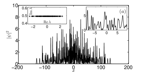
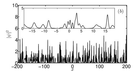
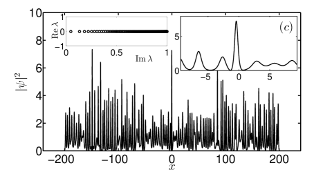
Figure 5: (Adapted from Gelash and Agafontsev (2018) and Gelash et al. (2019)) (a,c) Wave fields of $128$-SS constructed from solitons having uniformly distributed positions $x^{\mathrm{DM}}_{n}\in[-L_{0}/2,L_{0}/2]$, $L_{0}=2$, and phases $\theta^{\mathrm{DM}}_{n}\in[0,2\pi)$: (a) solitons have equal amplitudes $A_{n}=\pi/3.2\approx 1$ and Gaussian-distributed velocities with zero mean and standard deviation $V_{0}=2$, $V_{n}\sim\mathcal{N}(0,V_{0}^{2})$, and (c) solitons have amplitudes distributed according to the Bohr-Sommerfeld quantization rule for a rectangular box, see Eq. (70) below, and zero velocities $V_{n}=0$. (b) The wave field from panel (a) after placing it into the periodic box $x\in[-L_{p}/2,L_{p}/2]$, $L_{p}=128\pi$, and simulating the time evolution within the fNLS equation up to the final time $t=200$. Right insets in panels (a,c) and the inset in panel (b) show zoom of the wave fields. Left insets in panels (a,c) demonstrate soliton eigenvalues (note the swapped notations between the axes).

Figure 5 illustrates the “periodization” method on the example of a single $128$-SS generated from solitons having uniformly distributed positions $x^{\mathrm{DM}}_{n}\in[-L_{0}/2,L_{0}/2]$, $L_{0}=2$, and phases $\theta^{\mathrm{DM}}_{n}\in[0,2\pi)$, equal amplitudes $A_{n}=\pi/3.2\approx 1$ and Gaussian-distributed velocities with zero mean and standard deviation $V_{0}=2$, $V_{n}\sim\mathcal{N}(0,V_{0}^{2})$. The initial $128$-SS has characteristic size in the physical space $\delta X\simeq 280$, and in average the wave field is greater at the center than closer to the edges of the solution, see Fig. 5(a). Then, this solution is placed into the periodic box $x\in[-L_{p}/2,L_{p}/2]$, $L_{p}=128\pi$, and the evolution is simulated until the final time $t=200$, when the wave field in average becomes fairly uniform, see Fig. 5(b). As has been verified in Gelash and Agafontsev (2018), the soliton eigenvalues $\Lambda_{n}$ calculated at the final simulation time with the Fourier collocation method Yang (2010) almost coincide with the eigenvalues $\lambda_{n}$ of the initial $128$-SS with the relative differences between the two $|\lambda_{n}-\Lambda_{n}|/|\lambda_{n}|$ of $10^{-9}$ order.

The described above “periodization” method can be applied only when the soliton velocities are distributed over some finite interval of values. In Gelash et al. (2019), it has been observed that for the special case of bound-state soliton gas, i.e., when all solitons have the same velocity (which one can set to zero for simplicity), a certain distribution of soliton eigenvalues (i.e., amplitudes) leads to a statistically homogeneous multi-soliton wave fields in a wide region of the physical space for sufficiently small soliton positions $|x^{\mathrm{DM}}_{n}|\lesssim 1$ and random soliton phases; see Fig. 5(c). The figure shows $128$-SS constructed from solitons having zero velocity $V_{n}=0$ and uniformly distributed positions and phases over the intervals $x^{\mathrm{DM}}_{n}\in[-L_{0}/2,L_{0}/2]$, $L_{0}=2$, and $\theta^{\mathrm{DM}}_{n}\in[0,2\pi)$. The amplitudes are distributed according to the Bohr-Sommerfeld quantization rule, which is deduced from the solution of the direct scattering problem for the rectangular box potential; see Sec. VI.2 for detail. The resulting wave field turns out to be statistically homogeneous $\langle|\psi(x)|^{2}\rangle\approx 1$ over more than $70$% of its characteristic size in the physical space for random soliton phases Gelash et al. (2019). Cutting out the remaining $30$% at the edges where the wave field is not statistically homogeneous, one can use this $70$% part as a model of statistically homogeneous bound-state soliton gas. As discussed in Sec. VI.2, this soliton gas accurately models the long-time statistically stationary state of the noise-induced modulational instability of the plane wave solution.

We believe that there are other distributions of soliton amplitudes leading to the statistically homogeneous multi-soliton wave fields in a wide region of the physical space for sufficiently small soliton positions $|x^{\mathrm{DM}}_{n}|\lesssim 1$ and random soliton phases. The general question of constructing multi-soliton bound-state wave fields with a given profile $\langle|\psi(x)|^{2}\rangle=P(x)$ in the physical space and a given set of amplitudes $A_{n}$ by using random soliton phases and a specific distribution of soliton positions represents a challenging problem for future studies.

IV.3 Direct scattering transform analysis

In this subsection, we discuss the direct scattering transform (DST) analysis, which allows one to study the nonlinear composition of numerically or experimentally observed wave fields. Focusing only on the discrete spectrum (soliton eigenvalues and norming constants), we assume that the wave field in question is given in a simulation box $x\in[-L/2,L/2]$ and outside this box it equals zero. If the actual boundary conditions are different, then one can assume that the box $L$ is large enough compared to the characteristic sizes of nonlinear structures, so that the difference in the boundary conditions and the resulting edge effects can be neglected. Note that in this formulation the scattering coefficients $a(\lambda)$ and $b(\lambda)$ are analytic functions in the upper half of the $\lambda$-plane, that is essential for the algorithms discussed below.

In what follows, we describe the DST procedure presented in the recent study Agafontsev et al. (2023). This procedure, based on the standard DST methods Boffetta and Osborne (1992); Burtsev et al. (1998); Yang (2010) supplemented by the latest studies Mullyadzhanov and Gelash (2019); Gelash and Mullyadzhanov (2020); Mullyadzhanov and Gelash (2021) for the accurate calculation of the norming constants, contains several steps which are discussed below.

First, if there is a discontinuity of the wave field at $x=\pm L/2$, then it is smoothed using a smoothing window of the same size as the characteristic soliton width. It is assumed that the number of solitons inside the box $L$ is large and that these discontinuities, together with their smoothing, do not introduce significant inaccuracies in the results.

Second, an approximate location of the soliton eigenvalues is found using the standard Fourier collocation method Yang (2010). Being fast and fairly accurate, this method is based on the Fourier decomposition of the wave field, which artificially shifts the continuous spectrum eigenvalues to the upper half of the $\lambda$-plane due to the implied periodization. Also, it does not distinguish between the eigenvalues of discrete and continuous spectra, leading to the problem of identifying low-amplitude solitons.

Third, to cope this this problem, the wave field is considered in two larger boxes $x\in[-3L/4,3L/4]$ and $x\in[-L,L]$ by filling with zeros $\psi=0$ the intervals where the wave field is not defined. Then, the Fourier collocation method is executed in both boxes and only the eigenvalues coinciding in both calculations are selected as belonging to the discrete spectrum. While the latter provides a good approximation of the soliton eigenvalues, i.e., zeros of the coefficient $a(\lambda)$, this approximation is still insufficient for the accurate calculation of the norming constants, which requires knowledge of roots $a(\lambda_{n})=0$ to hundreds of digits Gelash and Mullyadzhanov (2020). That is why the calculated eigenvalues are then used as seeding values for a high-accuracy root-finding procedure.

The fourth and the final step of the described DST procedure consists in application of the standard second-order Boffetta–Osborne method Boffetta and Osborne (1992) on a fine interpolated grid using high-precision arithmetic operations, as suggested in Mullyadzhanov and Gelash (2019); Gelash and Mullyadzhanov (2020). The Boffetta–Osborne method is based on the calculation of the so-called extended $4\times 4$ scattering matrix $\mathbf{S}$, which translates the solution of the Zakharov–Shabat system $\mathbf{\Phi}$ together with its derivative $\mathbf{\Phi}^{\prime}=\partial\mathbf{\Phi}/\partial\lambda$ from $x=-L$ to $x=L$,

$$\begin{pmatrix}\mathbf{\Phi}(L)\\ \mathbf{\Phi}^{\prime}(L)\end{pmatrix}=\underbrace{\begin{pmatrix}\Sigma&0\\ \Sigma^{\prime}&\Sigma\end{pmatrix}}_{\mathbf{S}}\begin{pmatrix}\mathbf{\Phi}(-L)\\ \mathbf{\Phi}^{\prime}(-L)\end{pmatrix}.$$ (67)

Here $\Sigma(\lambda)$ is $2\times 2$ matrix, such that $\mathbf{\Phi}(L)=\Sigma(\lambda)\mathbf{\Phi}(-L)$, and the scattering coefficients are connected with the elements of matrix $\mathbf{S}$ as

$$a(\lambda) = S_{11}e^{2i\lambda L},\quad b(\lambda)=S_{21},$$

$$a^{\prime}(\lambda) = [S_{31}+iL(S_{11}+S_{33})]\,e^{2i\lambda L}.$$ (68)

Note that instead of the standard second-order Boffetta–Osborne method one can use the higher-order methods obtained with the Magnus expansion; see Mullyadzhanov and Gelash (2019, 2021) for detail. A fine spatial grid and the high-precision arithmetic operations are necessary to (i) neglect the round-off errors when calculating the wave function $\mathbf{\Phi}$ of the Zakharov–Shabat system, (ii) avoid the anomalous errors in computation of the norming constants, and (iii) suppress the numerical instability of the wave scattering through a large potential, see Mullyadzhanov and Gelash (2019); Gelash and Mullyadzhanov (2020) for detail. Also note that when avoiding the anomalous errors, one can supplement the DST procedure with the bidirectional algorithm and its improvements, see Prins and Wahls (2019), to decrease the necessary number of digits in the high-precision operations.

The Boffetta–Osborne method allows one to find the scattering coefficients $a(\lambda)$ and $b(\lambda)$ for any value of $\lambda$ by the direct numerical integration of the Zakharov–Shabat system on the interval $[-L/2,L/2]$ with boundary conditions (53). Note that $a(\lambda)$ and $b(\lambda)$ are analytic functions in the upper-half of the $\lambda$-plane, as the potential $\psi(x)$ has a compact support. Then, with the help of the Newton method, one can find roots $a(\lambda_{n})=0$ with the necessary precision by using the eigenvalues obtained by the Fourier collocation method as seeding values. Finally, the norming constants are calculated according to their definition (55) using the extended scattering matrix $\mathbf{S}$, see Eq. (68), to find the derivative $a^{\prime}(\lambda)$.

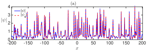
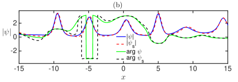
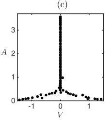
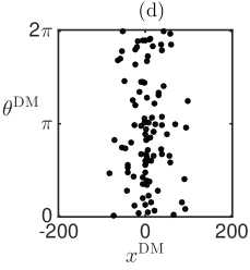
Figure 6: (Adapted from Agafontsev et al. (2023)) Numerical DST analysis of a periodic wave field that was “grown” from small statistically homogeneous in space noise within the fNLS equation, supplemented by a small linear pumping term, until the intensity, averaged over the simulation box, reached unity, $\overline{|\psi|^{2}}=1$; see Agafontsev et al. (2023) for details. Panel (a) shows the absolute values of the “grown up” wave field $|\psi|$ (solid blue) and the multi-soliton solution $|\psi_{s}|$ (dashed red); $\psi_{s}$ is constructed using the soliton parameters obtained in the DST procedure. Panel (b) represents zoom of panel (a), also demonstrating the complex phases of the “grown up” wave field (solid green) and the multi-soliton solution (dashed black). The dots in panels (c) and (d) illustrate soliton amplitudes $A_{n}$, velocities $V_{n}$, positions $x^{\mathrm{DM}}_{n}$ and phases $\theta^{\mathrm{DM}}_{n}$.

Figure 6 illustrates the performance of this DST procedure on the example of a periodic wave field that was “grown” from small statistically homogeneous in space noise within the fNLS equation, supplemented by a small linear pumping term, until the intensity, averaged over the simulation box, reached unity, $\overline{|\psi|^{2}}=1$; see Agafontsev et al. (2023) for details. The solid blue and green lines in Fig. 6(a,b) show the amplitude $|\psi|$ and complex phase $\mathrm{arg}\,\psi$ of the “grown up” wave field, while the dots in Fig. 6(c,d) demonstrate the calculated soliton amplitudes $A_{n}$, velocities $V_{n}$, positions $x^{\mathrm{DM}}_{n}$ and phases $\theta^{\mathrm{DM}}_{n}$. Using these soliton parameters, one can construct the corresponding exact multi-soliton solution as discussed in the previous subsection; it turns out that this solution approximates the original wave field very well, as illustrated by the dashed red and black lines in Fig. 6(a,b).

Note that the average intensity of the multi-soliton solution $\psi_{s}$ in Fig. 6 equals $99$% of that of the original “grown up” wave field $\psi$. Also, most of the solitons of this solution have zero velocities, forming a bound state. In Agafontsev et al. (2023), such a situation is observed if the initial noise amplitude and the pumping coefficient are small enough. If this is not the case, then the “grown up” wave fields with intensity of unity order $\overline{|\psi|^{2}}\sim 1$ also represent solitons-dominated states, which are not bound as these solitons have different velocities. Moreover, as shown in the paper, during the growth stage the solitonic part of the wave field becomes the dominant one very early when the average intensity is still small, $\overline{|\psi|^{2}}\simeq 0.1$, and the dispersion effects are leading in the dynamics. These observations indicate that the soliton gas model can be applicable even to weakly nonlinear cases, so that a soliton gas can be a very common object in nature.

V Experiments

From the experimental point of view, a few attempts to generate and to observe soliton gases have been made in some optical fiber experiments performed at the end of the 1990’s Schwache and Mitschke (1997); Steinmeyer et al. (1995); Mitschke et al. (1996). The soliton gas was generated by the synchronous injection of laser pulses inside a passive ring cavity. No direct observation but only averaged measurements of the Fourier power spectrum and of the second-order autocorrelation function characterizing the optical soliton gas have been reported in these pioneering experiments. Moreover, the dynamics of the ring resonator was so complex that many features ranging from purely temporal chaos to spatio-temporal chaos or turbulence were observed in this fiber system Mitschke et al. (1996).

Analysing ocean waves recordings, Costa et al. have reported the observation of random wavepackets in shallow water waves in 2014 Costa et al. (2014). The wavepackets have been analyzed using numerical tools of nonlinear spectral analysis Osborne et al. (2019b) and interpreted as being composed of random solitons that might be associated with KdV soliton gas. One year later, large ensembles of interacting and colliding solitons have been observed in a laboratory environment Perrard et al. (2015). The experimental system was a water cylinder deposited on a heated channel and levitating on its own generated vapor film owing to the Leidenfrost effect. Multiple soliton propagation was observed at the surface of the water cylinder and the Fourier analysis that was made in an attempt to characterize the multiple coherent structures revealed a “soliton turbulence-like spectrum”. Note also that a striking transition between weak turbulence and solitonic regimes has been evidenced in the hydrodynamic experiments reported in ref. Hassaini and Mordant (2017). In these experiments, water waves have been generated by exciting horizontally a water container by using an oscillating table. The weak turbulence regime observed at low forcing and/or large depth was shown to abruptly evolve into a solitonic regime at larger forcing and/or small depth. Remarkably, these results establish a possible link between the field of integrable turbulence and the field of wave turbulence.

In the recent laboratory experiments reported in ref. Redor et al. (2019), Redor et al. have taken advantage of the process of fission of a sinusoidal wave train to generate a bidirectional shallow water soliton gas in a 34-m long flume. The space-time observations have revealed complex dynamics where large numbers of colliding solitons retained their profile adiabatically, though their amplitude was slowly decaying because of some unavoidable damping. The Fourier analysis of the observed nonlinear wave field has clearly revealed the interplay between multiple solitons and dispersive radiation. Further analysis making use of the periodic scattering transform have been implemented in ref. Redor et al. (2021) to discriminate linear wave motion states from integrable turbulence and soliton gas. Moreover the statistical properties of the soliton gas have been given in terms of probability density distribution, skewness, and kurtosis Redor et al. (2021).

The experiments reported in ref. Redor et al. (2019, 2020, 2021) have been made in the presence of an unavoidable slow damping but it has been shown that a stationary state typified by the interplay among random bidirectional solitons can be achieved because of the continuous energy input by the wavemaker. In these shallow water experiments, a route to integrable turbulence has been discovered through the disorganization of wave motion that is induced by the wave maker Redor et al. (2021). This route has been shown to depend on the nonlinearity of the waves but also on the amplitude amplification and reduction due to the wavemaker feedback on the wave field Redor et al. (2021).

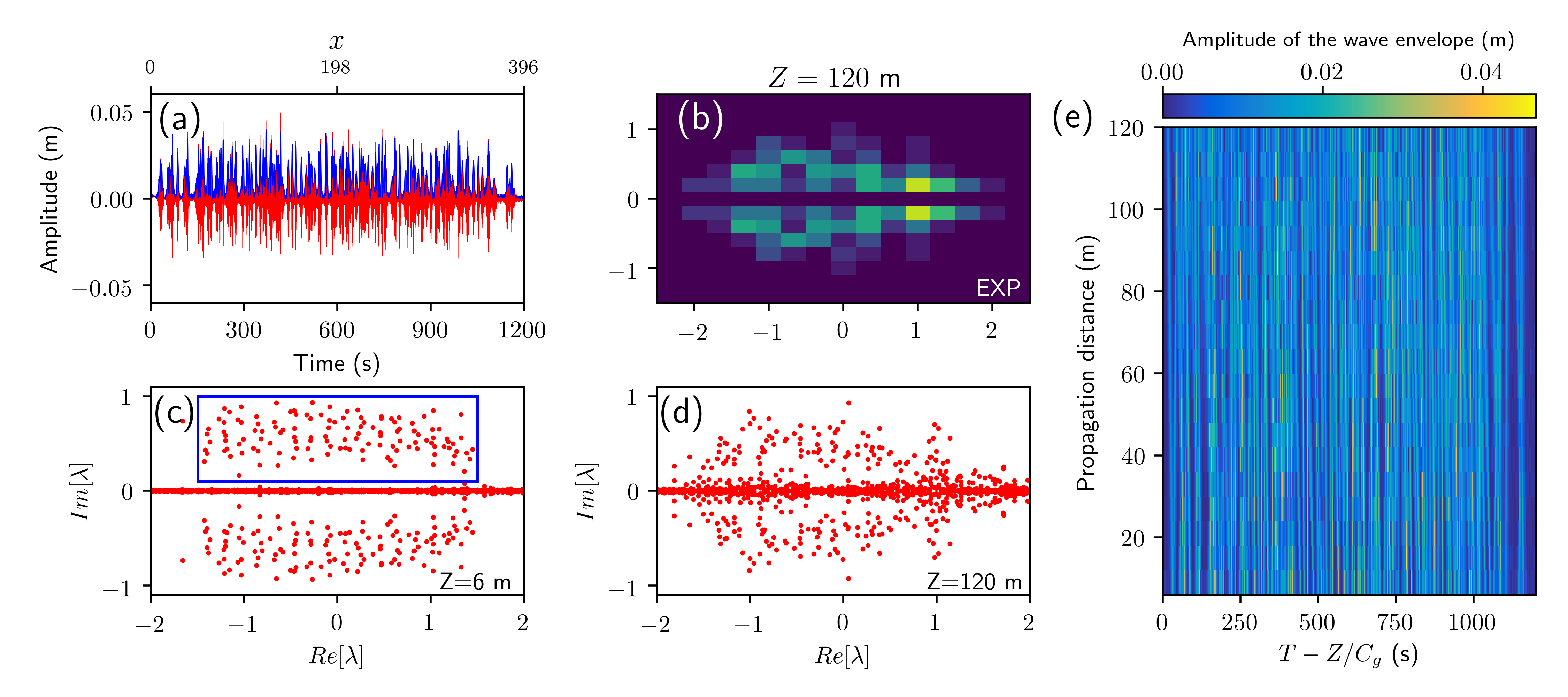
Figure 7: Gas of 128 solitons propagating in a 140-m long 1D water tank Suret et al. (2020). (a) Water elevation (red line) and modulus of the wave envelope measured at Z=6 m, close to the wave maker. (b) DOS of the soliton gas measured at Z=120 m. (c) Discrete IST spectrum measured at Z = 6 m. (d) Discrete IST spectrum measured at Z=120 m. (e) Space-time evolution of modulus of the wave envelope recorded by the 20 gauges regularly spaced along the tank. Reproduced with permissions from Suret et al. (2020)

Using an approach fully based on the IST method while also relying on the concept of DOS, a soliton gas has been generated in hydrodynamic experiments performed in the deep-water regime where wave propagation is described at leading order by the 1D fNLS equation Suret et al. (2020). The experiment has been performed in a wave flume being 148 m long, 5 m wide, and 3 m deep. Unidirectional waves have been generated at one end of the tank with a computer assisted flap-type wave maker and the flume is equipped with an absorbing device strongly reducing wave reflection at the opposite end. In these experiments the space-time evolution of the generated wave packet is measured with 20 gauges uniformly distributed along the tank.

The experiment reported in ref. Suret et al. (2020) starts from the numerical generation or synthesis of a soliton gas by using the methodology described in Sec. IV. An ensemble of $128$ solitons having spectral parameters being distributed in a rectangular region of the spectral IST plane has been numerically generated. The solitons have the modulus of their norming constants being equal to unity while their phases are randomly distributed between $-\pi$ and $+\pi$. In the experiment, the generated soliton gas has the form of a random wave field spreading over $\sim 1200$ s, see Fig. 7. It represents a dense soliton gas in where solitons are not isolated and not well separated like in a rarefied gas.

In the experiments reported in ref. Suret et al. (2020), a large number of discrete eigenvalues were distributed with some density within a limited region of the complex plane. This justifies the introduction of a statistical description of the spectral (IST) data. This represents a key point for the analysis of the observed wave field in the framework of the SG theory. In ref. Suret et al. (2020), the DOS of a homogeneous soliton gas has been measured for the first time in experiments, which provides an essential first step towards experimental verification of the kinetic theory of nonequilibrium SGs. Nonlinear spectral analysis of the generated hydrodynamic soliton gas reveals that the density of states slowly changes under the influence of perturbative higher-order effects that break the integrability of the wave dynamics.

VI Applications of soliton gases

Since the first paper of Zakharov Zakharov (1971), a peculiar interest has been ascribed to SG as a fundamental mathematical and physical concept. Importantly, it has been recently shown that SG theory can provide a powerful framework to describe theoretically the complex statistics underlying some well-known and fundamental nonlinear dispersive waves phenomena. It is indeed natural to expect that SG theory can be used to describe some specific regimes of integrable systems (integrable turbulence, see Sec. VI.1) Agafontsev and Zakharov (2015); Walczak et al. (2015); Soto-Crespo et al. (2016); Akhmediev et al. (2016); Suret et al. (2016); Michel et al. (2020); Tikan et al. (2018). In particular, by using numerical simulations, it has been shown in 2019 that the long-term statistical properties of the so-called spontaneous modulation instability coincides with those of a specifically-designed SG(see Sec.VI.2) Gelash et al. (2019). Very recently, the general relationship between the DOS of a SG and the kurtosis (second-order moment) of the waves has been derived (see Sec.VIII.2). This approach provides the first theoretical description of the long-term evolution of the noise-induced modulation instability and paves the way of the description of integrable turbulence by using SG theory.

VI.1 Integrable turbulence

Wave turbulence can be generally defined as the ensemble of all the complex phenomena emerging in random nonlinear waves systems. The phrase wave turbulence theory is often used in a more restrictive sense and is then defined as the statistical mechanics of weakly nonlinear and dispersive waves Nazarenko (2011b); Zakharov et al. (1992). The standard wave turbulence theory applies to non integrable waves systems in which the Physics at long-time is dominated by resonant interactions Picozzi et al. (2014). A general feature of wave turbulence is the exchange of energy among all the scales induced by the nonlinearity. If there is a source of energy for some given spatial scales (for example the large scales) and if other scales (for example small scales) are damped by dissipation, wave turbulence theory predicts the possible existence of the so-called Kolmogorov-Zakharov cascade. This corresponds to an out-of-equilibirum phenomenon characterized by a constant flux of energy between large and small scales Nazarenko (2011b); Zakharov et al. (1992); Picozzi et al. (2014). On the other hand, in the absence of energy source and of losses, if the wave system is Hamiltonian, nonlinear random waves may reach a thermodynamical equilibrium state (characterized by the equipartition of energy and the Rayleigh-Jeans distribution) Nazarenko (2011b); Zakharov et al. (1992); Picozzi et al. (2014); Pourbeyram et al. (2022); Suret (2022). Note that, in common wave systems, both the Kolmogorov-Zakharov and the Rayleigh-Jeans are characterized by power-lawed spectra.

The Physics of integrable waves systems is of profoundly different nature because of the infinite number of constants of motion and of the absence of resonances. In particular, nonlinear random integrable waves cannot reach the thermodynamical Rayleigh-Jeans equilibrium Picozzi et al. (2014); Suret et al. (2011). For this reason, Zakharov has introduced a new field of research, the integrable turbulence (IT), that is defined as the statistical description of integrable systems Zakharov (2009). Since this seminal paper in 2009, integrable turbulence has received a growing interest both from the theoreticalZakharov (2009); Zakharov and Gelash (2013); Pelinovsky et al. (2013b); Agafontsev and Zakharov (2015, 2016); Randoux et al. (2016); Zakharov et al. (2016); Dyachenko et al. (2016); Akhmediev et al. (2016); Soto-Crespo et al. (2016); Suret et al. (2017); Gelash et al. (2019); Didenkulova (2019); Xie et al. (2020); Agafontsev and Zakharov (2020) and experimental Walczak et al. (2015); Suret et al. (2016); El Koussaifi et al. (2018); Suret et al. (2017); Tikan et al. (2018); Kraych et al. (2019); Michel et al. (2020) points of view.

In practice, integrable turbulence corresponds to the propagation of random waves in systems described by integrable equations such as the 1D NLS, the KdV or the Sine-Gordon equations. In this Sec. VI, we focus on recent results on the 1DNLS integrable turbulence. The one dimensional focusing NLS equation provides a bridge between nonlinear optics and hydrodynamicsChabchoub et al. (2015); El Koussaifi et al. (2018). The 1D focusing NLS equation describes at leading order deep-water wave trains or optical fiber in anomalous dispersion regime and it plays a central role in the study of rogue waves Onorato et al. (2001, 2013); Akhmediev et al. (2013); Dudley et al. (2014, 2019). The relevent of approach to study nonlinear random waves is a statistical description, including probability density functions (PDF) of wave amplitude $\psi$ or of intensity $|\psi|^{2}$ and moments such as the kurtosis $\kappa_{4}=\langle|\psi|^{4}\rangle/\langle|\psi|^{2}\rangle^{2}$. The last years, the statistical properties of integrable turbulence has been widely studied by using numerical simulation of the NLS equations. Preserving integrability in long-term simulations is a delicate and challenging task, but to the best of the knowledge, integrable turbulence is characterized by stationary statistical properties of the field for long time $t$. This existence of a stationary statistical states in the long-time evolution of the waves system is the most fundamental known feature of integrable turbulence.

Integrable turbulence phenomena can be classified by considering the statistical properties of the initial conditions. Two classes of initial conditions have been extensively investigated : (i) the plane wave perturbed by a small random noise and, (ii) partially coherent waves.

The homogeneous solution of the 1D focusing NLS equation (the plane wave or condensate) is unstable in the presence of long wave perturbation. When the perturbation is a random process, this dynamical mechanism, known as the “noise-induced” or spontaneous modulation instability (MI) Agafontsev and Zakharov (2015); Toenger et al. (2015); Kraych et al. (2019), represents a prominent example of the integrable turbulence phenomena. Surprisingly, the long-term statistical state is characterized by a Gaussian local statistics of the field $\psi$ i.e. by a kurtosis $\kappa_{4}=2$ Agafontsev and Zakharov (2015) while the other statistical properties such as the Fourier spectra or two-points correlations are not trivial Kraych et al. (2019). These statistical quantities have been quantitatively measured in experiments but up to very recent studies, no theoretical description was available. In the Sec. VI.2, we show that the soliton gas concept provides a powerful theoretical tool to predict quantitatively the statistical properties of the long term evolution of the spontanesous modulation instability.

Partially coherent waves are random waves characterized by a finite typical spatial scale (or identically a finite typical spectral width). Partially coherent waves made of numerous statistically independent modes represent the standard ansatz for initial conditions in the wave turbulence theory Nazarenko (2011b); Picozzi et al. (2014) and exhibit Gaussian statistics. Such initial conditions have been extensively investigated in numerical simulations of defocusing and of focusing NLS equation and in experiments Randoux et al. (2014); Walczak et al. (2015); Suret et al. (2016); Randoux et al. (2016); El Koussaifi et al. (2018); Michel et al. (2020); Tikan et al. (2018). Starting with partially coherent waves initial conditions, the statistics deviates from Gaussian statistics as the time evolves and eventually reaches a heavy or a low tailed PDF in the focusing and defocusing regime respectively Randoux et al. (2016). The deviation from Gaussianity in the stationary statistical state increases together with the strength of the nonlinearity and, importantly, in the focusing regime, the strongest deviation is characterized by a kurtosis $k_{4}=4$ Agafontsev et al. (2021). Note that the higher is the kurtosis, the higher is the rate of emergence of extreme events (rogue waves).

The evolution of partially coherent waves in (non integrable) weakly nonlinear dispersive systems corresponds to the fundamental question of wave thermalization that has been widely investigated in wave turbulence theory. The evolution of the statistical properties of partially coherent waves in the framework of 1D NLS integrable turbulence can be described by using a non conventional wave turbulence theory approach Janssen (2003); Suret et al. (2011). This theoretical approach predicts the deviation from Gaussianity for a weak nonlinearity but is not valid in the high nonlinearity regime. In particular, up to now, the maximum value of the kurtosis $k_{4}=4$ was not understood. In Sec VIII.2, we summarize an extremely recent theoretical study which provides a demonstration of the maximum value of the kurtosis in the strongly nonlinear regime by using soliton gas theory.

It is important to note that soliton gas is a peculiar case of integrable turbulence. Indeed, in the framework of IST with zero boundary conditions, integrable turbulence can always be described by the combination of the discrete and of the continuous spectra. Our conjecture is that the high nonlinearity limit of integrable turbulence can always be described by purely solitonic solutions (soliton gas). We show in the Sec. VI.2 and important example illustrating this conjecture.

VI.2 Spontaneous Modulation Instability

The MI appears in many physical systems, such as deep water waves Osborne (2010), Bose-Einsteine condensates Strecker et al. (2002) or nonlinear optical waves Agrawal (2013). If the plane wave is perturbed by an initially small sinusoidal perturbation, the nonlinear stage of MI is described by homoclinic solutions of the 1D focusing NLS equation – the Akhmediev Breathers Akhmediev et al. (1985); Akhmediev and Korneev (1986); Akhmediev et al. (2009); Grinevich and Santini (2018). As reminded above, in the case of random initial perturbation, single-point statistics evolves toward a stationary Gaussian distribution (and $\kappa_{4}=\langle|\psi|^{4}\rangle/\langle|\psi|^{2}\rangle^{2}=2$.) despite the presence of highly nonlinear breather-like structures  Agafontsev and Zakharov (2015); Soto-Crespo et al. (2016); Akhmediev et al. (2016). The long-time (stationary) statistics is also typified by a quasi-periodic structure of the autocorrelation function $g^{(2)}$ of the wave field intensity Kraych et al. (2019).

In this section, we review numerical simulations that proves that the nonlinear stage of the spontaneous MI in the focusing regime of the Eq. 6 ($\sigma=+1$) can be quantitatively described by a specifically-designed soliton gas Gelash et al. (2019).

Without loss of generality, we consider the plane wave solution of Eq.6 – the condensate – of unit amplitude $\psi_{c}(t,x)=\exp{it}$. In the classical formulation of the spontaneous MI problem, the initial condition reads Zakharov and Ostrovsky (2009); Agafontsev and Zakharov (2015):

$$\psi(t=0,x)=1+\eta(x)\,,$$ (69)

where $\eta$ is a small noise, $\langle|\eta|^{2}\rangle\ll 1$, with zero average, $\langle\eta\rangle=0$. The destabilization of the condensate with respect to long-wave perturbations was widely investigated, both numerically by using periodic boundary conditions in a box of large size  Dudley et al. (2014); Toenger et al. (2015); Agafontsev and Zakharov (2015); Kraych et al. (2019), and experimentally Närhi et al. (2016); Kraych et al. (2019); Lebel et al. (2021). The typical spatio-temporal dynamics of the spontaneous MI can be seen in Fig. 8.a.

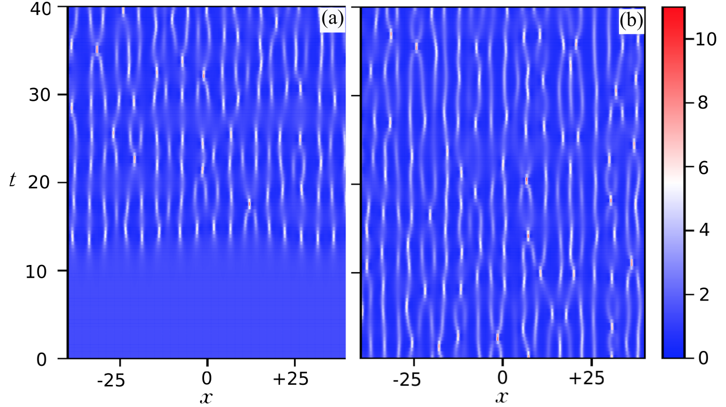
Figure 8: Numerical simulations of the one dimensional focusing NLS equation : Space-Time diagrams of $|\psi(x,t)|^{2}$ (a) Noise-induced Modulational Instability of a plane wave (periodic boundary conditions). (b) Dynamics of the random phase bound $N$-SS (only the central part of the $N$-SS having a total width $L_{0}\simeq 400$ is plotted).
Reproduced with permission from Gelash et al. (2019)

In order to demonstrate that the statistical properties of the spontaneous MI coincide at long-time with the ones of SG, the first step used in Gelash et al. (2019) is to modify the boundary conditions. The idea is that if one fixes the time at which the nonlinear stage of MI is characterized (typically $t>30$ in Fig. 8.a), the plane wave with periodic boundary condition can be replaced by a box with ZBC. The width of the box has to be sufficiently large to avoid any influence of the edges in the central part of the box at the considered time $t$.

By using the same idea, one expects that any homogeneous SG can be locally modeled by a N-SS (with zero boundary conditions). Moreover, in order to model the long-time dynamics of a stochastic field, it is natural to assume random norming constants phases because the phase rotations $-2i\lambda_{n}^{2}t$ for large $t$ introduce an effective randomization. Note that somehow, this random phases of the norming constant are similar to the so-called “random phase approximation” (i.e. random phases of the Fourier components) in wave turbulence theory Zakharov et al. (1992); Nazarenko (2011b).

Finally, the last step is to determine the DOS. of the SG underlying the dynamics of the field. Here, the answer is rather simple because the discrete spectrum of a real-valued rectangular box of unit amplitude and width $L_{0}$ is known. In the limit $L_{0}\gg 1$, the discrete spectrum of the semi-classical Zakharov-Shabat scattering problem is given by the Bohr-Sommerfeld quantization rule, see e.g. Zakharov and Shabat (1972); Novikov et al. (1984) and also Lewis (1985b):

$$\lambda_{n}=i\,\beta_{n}=i\,\sqrt{1-\left[\frac{\pi(n-\frac{1}{2})}{L_{0}}\right]^{2}},\quad n=1,2,\dots,N,$$ (70)

where $N=\hbox{int}[L_{0}/\pi]$ (the density of the gas, i.e. the number of solitons per unit length is thus $1/\pi$). The continuus limit of Eq. (70) with $N\to\infty$, $\beta_{n}\to\beta$ gives the normalized distribution $\varphi(\beta)$ of the IST eigenvalues:

$$\varphi(\beta)=\frac{1}{N}\frac{dn}{d\beta}=\frac{\beta}{\sqrt{1-\beta^{2}}}$$ (71)

which appears to be the so-called Weyl distribution. Finally, here, the DOS is simply:

$$f(\beta)=\frac{1}{L_{0}}\frac{dn}{d\beta}=\frac{1}{\pi}\varphi(\beta).$$ (72)

This is nothing but the 1D focusing NLS bound state soliton gas DOS (48) obtained in Section III.4 as the solution of the NDRs (41) in the limit $\sigma\to 0$ assuming the spectral support $\Gamma^{+}=[0,i]$. In Gelash et al. (2019) a large number of realizations of N-SSs that fulfil the required eigenvalues distribution given by the Eq. 71 have been computed with random phase for the norming constants by using the procedure described in Sec.IV.2. This realizations ensemble models a bound SG in the limit $N$ large ($N=128$ in  Gelash et al. (2019)). As the N-SS are bound states (Re $\lambda_{n}=0$), the expected dynamics of the wave field is identical to the dynamics observed in the nonlinear stage of the spontaneous MI. Indeed, the zero-velocity of the solitons prevent any dilution of the gas during the evolution.

The Fig. 8 displays the comparison between two NLS equation simulations made with different initial conditions: Fig. 8.a corresponds to the dynamics of the plane wave (initially pertubed with noise) while Fig. 8.b corresponds to the dynamics of one realization of the $N$-SS. The features characterizing the spatio-temporal dynamics of the long-time evolution of the plane wave (typically for time $t>20$) seams very similar to the one of the $N$-SS. As expected, the specifically-designed $N$-SS apparently is a very good model of the nonlinear stage of the spontaneous MI.

More importantly, the statistical properties of SG coincide in a quantitative manner with those of the asymptotic stage of MI. For example, the long-term evolution of the noise-induced MI is characterized by stationary values the potential $H_{nl}$ and kinetic $H_{l}$ energy Agafontsev and Zakharov (2015), $\langle H_{l}\rangle=0.5$ and $\langle H_{nl}\rangle=-1$ where the total energy (Hamiltonian) $H$, which is one of the infinite constants of motion of the 1D-fNLS equation Novikov et al. (1984) reads

$$H=H_{l}+H_{nl},\quad H_{l}=\frac{1}{2}\frac{1}{L}\int_{-L/2}^{L/2}|\psi_{x}|^{2}\,dx,$$

$$H_{nl}=-\frac{1}{2}\frac{1}{L}\int_{-L/2}^{L/2}|\psi|^{4}\,dx.$$ (73)

The Fig. 9 shows the comparison between three other statistical of both the long-time evolution of the spontaneous MI and of the ensemble of $N$-SS. The Fig. 9.a displays the wave-action spectrum,

$$S_{k}\propto\langle|\psi_{k}|^{2}\rangle,\quad\psi_{k}=\frac{1}{L}\int_{-L/2}^{L/2}\psi\,e^{-ikx}\,dx.$$ (74)

The Fig. 9.b displays the probability density function (PDF) $\mathcal{P}(I)$ of the field intensity $I=|\psi|^{2}$ which is known to follow the exponential distribution in the asymptotic statistics of the unstable condensate Agafontsev and Zakharov (2015); Kraych et al. (2019). Finally, the Fig. 9.c displays the autocorrelation of the intensity $g^{(2)}(x)$ :

$$g^{(2)}(x)=\frac{\bigl{\langle}I(y,t)I(y-x,t)\bigr{\rangle}}{\bigl{\langle}I(y,t)\bigr{\rangle}^{2}}$$ (75)

which represents the second-order degree of coherence.

Remarkably, all these statistical quantities computed in the asymptotic state of the MI coincide with excellent accuracy with those of the considered SG. In addition, further studies revealed that extreme amplitude waves emerging in the asymptotic state of the MI and the soliton gas have identical dynamical and statistical characteristics Agafontsev and Gelash (2021). Note that this agreement is weakly depend on the exact eigenvalues chosen for the $N$-SS because the key ingredient are the statistical distribution of the eigenvalues and the use of random phases for the norming constants (in other words, similar statistical results have been obtained in the case of soliton eigenvalues randomly distributed according to the probability function (71) Gelash et al. (2019).

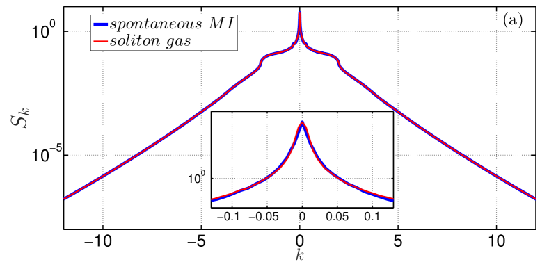
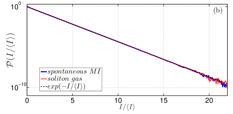
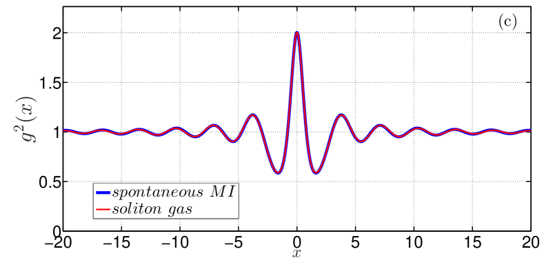
Figure 9: Comparison of ensemble averaged statistical characteristics of the asymptotic state of the MI development and of random phase $128$-SSs. (a) Wave action spectrum $S_{k}$. (b) The PDF $\mathcal{P}(I)$. (c) Autocorrelation function of intensity (second order degree of coherence) $g^{(2)}(x)$. Reproduced with permission from Gelash et al. (2019).

What are the main conclusions of this numerical study? First, the asymptotic state of the spontaneous MI can be modeled as a specific SG – the bound state soliton condensate. This SG can be constructed with exact $N$-SSs of the one dimensional focusing NLS equation by using large values of $N$ and the Weyl’s distribution of IST eigenvalues coinciding with the one predicted for the box potential in the semi-classical limit Zakharov and Shabat (1972). Moreover, the long-term statistical state of MI corresponds to a full stochastization of the phases of the norming constants i.e. the solitons’ phases. Finally, note that for other distributions of eigenvalues tried by the authors, the statistical properties of the SG do not coincide with the ones of the MI and/or are strongly non homogeneous in space Gelash et al. (2019).

These results open a promising direction in the theory of integrable turbulence by establishing a link between the MI and SGs dynamics. It is important to note that this quantitative link is possible in the case of MI because for a “semi-classical” box, the contribution of the “non-soliton” part of the field, i.e. of the continuous IST spectrum, decays exponentially with $L_{0}$ and so can be neglected Novikov et al. (1984). As a consequence, this modeling of integrable turbulence by using SG can be a priori generalized to a broad class of IT problems when the (random) wave field is strongly nonlinear, so that the impact of the non-solitonic content can be neglected in the asymptotic state ($t\to\infty$). For such a case, the general strategy to study the asymptotic state should be to build $N$-soliton solutions with the distribution $\varphi(\lambda)$ of IST eigenvalues characterizing the field and random phases of the norming constants (see Sec.VIII.2). We review in Section VIII.2 new results showing that this approach provides a a framework allowing to compute theoretically the observed value of $\kappa=2$ for the long term evolution in the spontaneous MI phenomenon Kraych et al. (2019) and $\kappa=4$ for the semiclassical limit of partially coherent waves Agafontsev et al. (2021).

VII Generalized hydrodynamics

VII.1 The perspective of emergent hydrodynamics

As mentioned, it is very natural to understand the theory of soliton gases within a kinetic perspective, as the fundamental objects – the soliton DOS or phase-space density $f(\eta;x,t)$ introduced in Section II, its the kinetic equation, Section II.3.2, and the equation of state for the effective velocity $s(\eta;x,t)$, Eq. (17) – have a clear kinetic interpretation in terms of soliton propagation and scattering. This interpretation is mathematically accurate at low densities, but at high densities, although compelling, it remains nebulous. The kinetic viewpoint is in fact an a-posteriori interpretation: as reviewed in Section III, the soliton gas theory may be derived from an appropriate thermodynamic limit of finite-gap (quasi-periodic) solutions and its Whitham modulations.

Independently from the soliton gas theory, a framework for the emergent large-scale behaviours of quantum many-body integrable systems out of equilibrium was more recently developed, dubbed “generalised hydrodynamics” (GHD) Castro-Alvaredo et al. (2016); Bertini et al. (2016). In this context, the problem is to determine the dynamics of quantum systems, such as the Lieb-Liniger gas Lieb and Liniger (1963) and Heisenberg quantum spin chain Faddeev (1996), out of equilibrium. One seeks, for instance, the full space-time profile of expectation values of local observables, from an initial state that present variations on large scales; or the full space-time profile of their correlation functions. As it was realised Doyon et al. (2018a), it turns out that the main objects of GHD – the phase-space densities denoted in this context $\rho_{\rm p}(\eta;x,t)$, the kinetic equation reffered to as the “GHD equation”, and the equation of state for the effective velocity denoted $v^{\rm eff}(\eta;x,t)$ – have exactly the same structure as in soliton gases. The spectral parameter $\eta$ is identified with the quasi momentum of the thermodynamic Bethe ansatz (TBA), and quite surprisingly the two-body scattering shift is simply identified with the semiclassical shift of quantum wavepackets, or the “kernel” of the TBA equations. The TBA Lieb and Liniger (1963); Yang and Yang (1969); Zamolodchikov (1990); Takahashi (1999); Mossel and Caux (2012) is a framework first developed at the beginning of the 1960’s to construct the thermodynamics of Bethe-ansatz integrable systems.

However, by contrast to the theory of soliton gases, in GHD a different viewpoint is emphasised. Certainly, a kinetic perspective can be taken, as was done in one of the co-founding papers of GHD Bertini et al. (2016): “Bethe quasiparticles” are the kinetic objects, and the effective velocity $v^{\rm eff}(\eta)$ had in fact been proposed earlier Bonnes et al. (2014) as their emergent propagation velocity within finite-density states. However, in the quantum context it is more difficult to establish the validity of this perspective, even at low densities. Further, a quantum modulation theory has not yet been developed. Instead, the currently prevalent viewpoint, emphasised in the other co-found paper of GHD Castro-Alvaredo et al. (2016), is that of the emergence of hydrodynamics at large spacetime scales. This physical idea implies that the structure of GHD is in fact that of Euler equations, instead of a kinetic theory, only generalised to infinitely-many conservation laws.

Euler hydrodynamics is the idea that locally, within each “mesoscopic” region of space and time (sometimes referred to as “fluid cell”), the system’s state looks as if it had relaxed. A mesoscopic spacetime region covers a length that is large as compared to the microscopic scales (the inter-particle scales and interaction distances) but small as compared to macroscopic scales (the length scales at which averages of local observables show variations); and a time that is likewise large compared to microscopic, and small compared to macroscopic, times. According to conventional physical wisdom, a state that has “relaxed” is spacetime stationary and takes the Gibbs form. Thus, in Euler hydrodynamics, one assumes that at every point in space-time, the state looks like it is in Gibbs form. The Gibbs form arises from an entropy maximisation principle, so these are “maximal entropy states”, and we may therefore talk about “local entropy maximisation”. The local maximal entropy states depends on space-time, and upon imposing all the available local conservation laws, this gives the Euler equations for the system.

It has been worked out in the past 20 years (see the reviews Essler and Fagotti (2016); Vidmar and Rigol (2016)) that the so-called Generalised Gibbs Ensembles (GGE), with density matrix

$$\mbox{GGE:}\quad\rho\propto e^{-\sum_{i}\beta_{i}Q_{i}}$$ (76)

where $Q_{i}=\int dx\,q_{i}(x,t)$, with $\frac{dQ_{i}}{dt}=0$, are extensive conserved quantities, correctly describe relaxation in many-body integrable models. In the infinite-volume limit, infinitely many conserved quantities $Q_{i}$ must be considered (under some convergence condition). The emergent hydrodynamic perspective then simply states that the local MES are GGEs, so the local relaxation process is

$$\langle o(x,t)\rangle_{\text{initial state}}\to\langle o\rangle_{{\rm GGE}(x,t)}$$ (77)

for “any” local observable $o(x,t)$. Here GGE$(x,t)$ is described by “Lagrange parameters” $\beta_{i}(x,t)$ which depend on space-time. In the hydrodynamic approximation, the GGEs only depend slowly on space and time, and one then imposes the local conservation laws $\partial_{t}q_{i}(x,t)+\partial_{x}j_{i}(x,t)=0$ for GGE-average local densities $q_{i}(x,t)$ and their currents $j_{i}(x,t)$, in order to obtain the long-wavelength, slow dynamics,

$$\frac{\partial}{\partial t}\langle q_{i}\rangle_{{\rm GGE}(x,t)}+\frac{\partial}{\partial x}\langle j_{i}\rangle_{{\rm GGE}(x,t)}=0.$$ (78)

In principle, barring subtleties associated to hyperbolic systems of equations (see for instance Bressan (2013)), these are enough equations to have a well-posed initial value problem. The crucial ingredient in (78) is the “thermodynamic equations of state”: the way the average currents $\langle j_{i}\rangle_{\rm GGE}$ are related to the average densities $\langle q_{i}\rangle_{\rm GGE}$. Once this is known explicitly, the hydrodynamic equation (78) is written explicitly.

Thus, the usual ideas of hydrodynamics are simply extended to the principle of “generalised thermalisation” for many-body integrability; this is the hydrodynamic basis for GHD, justifying its name.

VII.2 The thermodynamic Bethe ansatz

In the hydrodynamic perspective, no kinetic theory is invoked. This perspective emphasises not the kinetic interpretation of the equations, but rather their thermodynamic and hydrodynamic interpretations. But how does one deal with infinitely-many conservation laws, and a large space of maximal entropy states? And how does a formulation that looks like a kinetic theory emerge?

This is thanks to the structure of the TBA. In order to describe it, take the integrable model of Bose particles interacting with a delta-function potential, the repulsive Lieb-Liniger gas Lieb and Liniger (1963) (see the review Bouchoule and Dubail (2022) where its GHD is explained),

$$H=-\sum_{n=1}^{N}\frac{1}{2}\frac{\partial^{2}}{\partial x_{n}^{2}}+\sum_{n<m=1}^{N}c\delta(x_{n}-x_{m}),\quad c>0.$$ (79)

The fully symmetric $N$-particle Bethe ansatz eigenfunctions, parametrised by Bethe roots $\eta_{n}$’s, take the form

$$\Psi(\{x\})\propto\sum_{\mathcal{P}:\text{permutations}}\ \prod_{n<m}{\rm sgn}\,(x_{{\mathcal{P}}(n)}-x_{{\mathcal{P}}(m)})\,\exp[\\ {\rm i}\sum_{n}\eta_{n}x_{\mathcal{P}(n)}+\frac{\rm i}{4}\sum_{n\neq m}\phi(\eta_{n}-\eta_{m})\,{\rm sgn}\,(x_{\mathcal{P}(n)}-x_{\mathcal{P}(m)})\Big{]}.$$ (80)

The quantity $\phi(\eta_{n}-\eta_{m})=2\,{\rm Arctan}\,\frac{\eta_{n}-\eta_{m}}{c}$ is the two-body quantum scattering phase shift occurring when a particle of Bethe root $\eta_{n}$ scatters with one of Bethe root $\eta_{m}$. Conserved quantities (including the Hamiltonian) take a simple form on these eigenfunctions:

$$Q_{i}\Psi(\{x\})=\sum_{n=1}^{N}h_{i}(\eta_{n})\Psi(\{x\})$$ (81)

where the functions $h_{i}(\eta)$ are the “one-particle eigenvalue”. These include the total number of particle $Q_{0}$ (with $q_{0}(x)=\sum_{n}\delta(x-x_{n})$ and $h_{0}(\eta)=1$), the momentum $Q_{1}$ (with $q_{1}(x)=\frac{1}{2}\sum_{n}-{\rm i}\{\partial_{x_{n}},\delta(x-x_{n})\}$ and $h_{1}(\eta)=\eta$), and the energy $Q_{2}=H$ (with $h_{2}(\eta)=\eta^{2}/2$). In fact, local conserved charges – those admitting a local density $q_{i}(x,t)$ – have $h_{i}(\eta)\propto\eta^{i}$ for all $i\in\mathbb{N}$. In a system of finite length $L$, the values of $\eta_{n}$’s are quantised as is usual in quantum mechanics; however the quantisation condition is nontrivial: these are the Bethe ansatz equations, involving $\phi(\eta)$ (see for instance Bouchoule and Dubail (2022)).

The TBA is based on the basic statistical mechanics principle of the equivalence of the microcanonical and macrocanonical ensembles, but generalised to all conserved charges, or equivalently all Bethe roots. Thus, the sum over eigenstates involved in a GGE concentrates on a fixed distribution of Bethe roots $\rho_{\rm p}(\eta)$, and one evaluates GGE averages of conserved densities by using this distribution, $\langle q_{i}\rangle_{{\rm GGE}}=\int d\eta\,\rho_{\rm p}(\eta)h_{i}(\eta)$, as follows from (81). The TBA gives an explicit map from $\beta_{i}$’s to $\rho_{\rm p}(\eta)$. This map is obtained by minimising a free energy functional that encodes the constraints on quasi-momenta arising from the Bethe ansatz equations. The result may be written in the suggestive form

$$\varepsilon(\eta)=\sum_{i}\beta_{i}h_{i}(\eta)-\int\frac{d\eta^{\prime}}{2\pi}\,\varphi(\eta-\eta^{\prime})\log(1+e^{-\varepsilon(\eta^{\prime})}),\\ \quad\rho_{\rm p}(\eta)=-2\pi\frac{\partial}{\partial\beta_{0}}\log(1+e^{-\varepsilon(\eta)})$$ (82)

involving the pseudoenergy $\varepsilon(\eta)$, defined as the solution of the above non-linear integral equation, and the differential scattering phase, defined by

$$\varphi(\eta)=\frac{d\phi(\eta)}{d\eta}=\frac{2c}{\eta^{2}+c^{2}}.$$ (83)

In this sense, the phase-space density $\rho_{\rm p}(\eta;x,t)$ does not arise as a density for particle-like dynamical objects forming a gas, but rather as a way of characterising all averages of local conserved densities in the $x,t$-dependent GGE that arises from the Euler hydrodynamic principle,

$$\langle q_{i}\rangle_{{\rm GGE}(x,t)}=\int d\eta\,\rho_{\rm p}(\eta;x,t)h_{i}(\eta).$$ (84)

Many-body integrable systems admit an infinite-dimensional space of conserved quantities $Q_{i}$, and the spectral parameter is just seen as a continuous parametrisation of this space (interpreted as a particular choice of a “scattering basis”, see e.g. the discussion in Nardis et al. (2022)).

As mentioned above, the crucial ingredient is the relation between GGE averages of currents and densities. Historically, this was in fact the main stumbling block in developing the hydrodynamics of integrable systems.

Average currents in GGE were first evaluatedCastro-Alvaredo et al. (2016) using the TBA and crossing symmetry of relativistic quantum field theory; they were later derived directly from the Bethe ansatz and other quantum integrability techniques Vu and Yoshimura (2019); Pozsgay (2020), and then from “self-conserved” currents Spohn (2020); Yoshimura and Spohn (2020), using the symmetry of current-charge correlations Castro-Alvaredo et al. (2016); Nardis et al. (2019); Karevski and Schütz (2019); see the reviews Borsi et al. (2021); Cubero et al. (2021). The result is striking: it takes the form

$$\langle j_{i}\rangle_{{\rm GGE}(x,t)}=\int d\eta\,v^{\rm eff}(\eta;x,t)\rho_{\rm p}(\eta;x,t)h_{i}(\theta)$$ (85)

where the effective velocity, here obtained, we recall, via Bethe ansatz calculations, satisfies the classical-looking collision rate ansatz (17), with $G(\eta,\eta^{\prime})=-\varphi(\eta-\eta^{\prime})$ and $s_{0}(\eta)=\eta$

$$v^{\rm eff}(\eta)=\eta+\int d\mu\,\varphi(\eta-\mu)\rho_{\rm p}(\mu)(v^{\rm eff}(\mu)-v^{\rm eff}(\eta)).$$ (86)

Its $x,t$ dependence $v^{\rm eff}(\eta)\to v^{\rm eff}(\eta;x,t)$ comes from the $(x,t)$-dependent GGE $\rho_{\rm p}(\eta)\to\rho_{\rm p}(\eta;x,t)$. Note how the differential scattering phase $\varphi(\eta-\eta^{\prime})$, Eq. (83), arises: this is exactly the semiclassical scattering shift of Bethe ansatz wave packets. One then obtains, from (78) and assuming some completeness of the space of functions $h_{i}(\theta)$, the GHD equation

$$\frac{\partial}{\partial t}\rho_{\rm p}(\eta;x,t)+\frac{\partial}{\partial x}\big{(}v^{\rm eff}(\eta;,x,t)\rho_{\rm p}(\eta;x,t)\big{)}=0.$$ (87)

This is, in this perspective, a Euler hydrodynamic equation, even though it looks like a kinetic equation.

We finally note that each value of the spectral parameter $\eta$ corresponds to a hydrodynamic normal mode – a “sound mode” or the like – for the emergent Euler-scale equation, and $v^{\rm eff}(\eta;x,t)$ are the associated hydrodynamic velocities tangent to their characteristics. Riemann invariants can be explicitly constructed; indeed $\varepsilon(\eta;x,t)$, or any function of it, satisfies the diagonalised Euler-scale equation, $\partial_{t}\varepsilon(\eta;x,t)+v^{\rm eff}(\eta;x,t)\partial_{x}\varepsilon(\eta;x,t)=0$, and so does the “cumulative density” or height field $\int_{-\infty}^{x}dx^{\prime}\,\rho_{\rm p}(\eta;x^{\prime},t)$; likewise, for linear perturbations on top of a homogeneous stationary background, $\rho_{\rm p}(\eta)+\delta\rho_{\rm p}(\eta;x,t)$, we have $\partial_{t}\delta\rho_{\rm p}(\eta;x,t)+v^{\rm eff}(\eta)\partial_{x}\delta\rho_{\rm p}(\eta;x,t)=0$.

VII.3 Universality of Euler hydrodynamics

Note that, curiously, one obtains, using the above description, a re-interpretation of the Liouville equation of phase-space conservation in classical mechanics. Traditionally it is understood in kinetic theory as a “collisionless” Boltzmann equation. Now take, for instance, the Tonks-Girardeau limit $c\to\infty$, where the Lieb-Liniger model becomes a model of non-integracting fermions, with $\varphi(\eta)=0$. The resulting GHD equation is the Liouville equation. But here, it is seen as a hydrodynamic equation, for a continuum of sound modes emerging at large scales in this system of non-interacting particles! The same hold for any system of non-interacting particles, quantum or classical.

This latter observation leads us to emphasise an important concept: the hydrodynamic perspective has the advantage that it is indifferent to the precise nature of the underlying many-body system. It has a large amount of universality.

This universality arises at two levels. First, the general structure of hydrodynamics at the Euler scale is always the same, no matter the underlying many-body system, under fairly general conditions (local interactions, and perhaps microscopic reversibility). The important point in establishing the Euler-scale hydrodynamic theory of a given many-body system is to characterise its full manifold of maximal entropy states. One expects that the “extensive conserved quantities”, widely studied in quantum many-body systems Ilievski et al. (2016), span the tangent spaces to this manifold, and according to Euler hydrodynamics, their densities are the emergent dynamical degrees of freedom onto which the microscopic dynamics projects at large scales; at the linearised level, this phenomenon has been rigorously established in quantum spin chains Doyon (2022) and lattices D. and Doyon (2022). Once the space of extensive conserved quantities is understood, the hydrodynamic principles – local relaxation and the conservation laws – are completely general, and do not require any strong dynamical assumptions such as chaos, or any particular structures for the underlying microscopic theory.

Second, within the family of many-body integrable models, the description of Section VII.2 is also completely universal. The microscopic system may be quantum or classical, composed of continuous fields, particles, solitons, spins, etc. – the same structure emerges for its Euler-scale hydrodynamics. The model-dependent aspects are the phase space $\mathcal{S}$ of possible values of the spectral parameter $\eta$ (it is $\mathbb{R}_{>0}$ in the KdV soliton gas, $\mathbb{R}$ in the repulsive LL model, $\mathbb{C}$ in the soliton gas of focusing NLS, etc.), and the basic dynamical quantities, including the two-body shift $G(\eta,\mu)$ (it is $-\frac{2c}{(\eta-\mu)^{2}+c^{2}}$ in the repulsive LL model, $\frac{1}{\eta}\log|\frac{\eta+\mu}{\eta-\mu}\big{|}$ in the KdV soliton gas, etc.), as well as a “bare” velocity $s_{0}(\eta)$ entering as the source term in the equations of state, Eqs. (17), (16), (86) ($\eta$ in the LL model, $4\eta^{2}$ in the KdV soliton gas, etc.). Thus, in fact GHD is not only a theory for many-body quantum integrable systems, but also for classical systems, including soliton gases. The full equivalence between TBA quantities and those of soliton gases is given in T et al. (2022).

This universality of the hydrodynamic description of integrable models has its source in an important aspect of many-body integrability, that of factorised, elastic scattering. Factorised scattering for solitons was reviewed in Section II.1, see Eq. (5). It is also made apparent in the LL Bethe ansatz wave function (80): the structure in the exponential implies that the phase of a full many-particle scattering is the sum of two-body scattering phases. If we put the LL model in a finite segment and let the particles expand in the vacuum, then $\eta_{n}$’s are the values of asymptotic momenta that will be seen at long times in this time-of-flight “gedenkenexperiment”. In general, for both quantum and classical models, the spectral space is nothing else than the set of possible objects that emerge at long times (solitons, particles, bound states, waves, etc.), and a basic dynamical analysis will give the bare velocities and two-body scattering shifts for such objects. It turns out that TBA form of the thermodynamics then emerges quite generally solely from this scattering picture; in classical systems this was first observed Doyon (2019) in the Toda model – thus the TBA does not require the Bethe ansatz! In a fluid, a mesoscopic cell can be “observed” by taking it out of the fluid and making a time-of-flight experiment on it, in order to determine the distribution of spectral parameters that characterise it. The manifold of GGEs is a manifold of distributions on the spectral space. In particular, the soliton gas is simply the case where we restrict the manifold of GGEs to be distributions of solitons only; and this restriction is stable under the Euler hydrodynamic evolution. This explains the general structure of GHD.

In fact, the scattering picture has far-reaching ramifications. One of them is the geometric viewpoint on GHD, whereby the GHD equations are seen as arising from a change of coordinates – or a change of metric – from the free-particle Liouville equations Doyon et al. (2018b); Doyon (2020). The change of metric is state-dependent (much like in Einstein’s gravity!), and represents the map to the freely-propagating asymptotic coordinates. This leads to an integral-equation solution Doyon et al. (2018b), a “solution by characteristics” akin to the hodograph transform.

VIII Open questions

Over the last few years, various fundamental questions inspired by the exciting theoretical and experimental challenges have emerged in the growing fields of SGs and of GHD. We summarize here some of the most important of these open questions.

VIII.1 Spectral theory and rigorous asymptotics

The spectral theory of soliton gas outlined in Secton III is based on the thermodynamic limit of finite-gap potentials and their Whitham modulation equations. At the core of this theory is the special distribution (scaling) of finite-gap spectra ensuring appropriate balance of terms in the nonlinear dispersion relations. Can this thermodynamic spectral scaling be obtained as a long-time asymptotics in some class of initial-value problems for integrable equations? One possible scenario to be explored was proposed in El et al. (2016) where one considers a chain of topological bifurcations of local invariant tori parametrized by slowly evolving finite-gap spectra that emerge in the zero-dispersion (semi-classical) limit of the fNLS equation. This scenario resembles the classical Landau-Hopf transition to turbulence (see e.g. Landau and Lifshitz (1987)) realized in the framework of an integrable dispersive system.

A related major open question is a rigorous mathematical justification of the spectral kinetic theory. The derivation of the kinetic equation via the thermodynamic limit of finite-gap modulation theory is formal in the sense that the question of the asymptotic validity of the kinetic equation in the framework of the original nonlinear dispersive PDE remains open. It would be highly desirable to have a rigorous asymptotic derivation of the kinetic equation for KdV, NLS and other integrable models. An important step in this direction has been recently made in ref. Girotti et al. (2022) where it was shown that kinetic equation for soliton gas describes the leading order asymptotic behaviour of a special class of “deterministic” soliton gases for the modified KdV equation constructed as an infinite-soliton limit of $N$-soliton solutions by invoking the theory of the so-called primitive potentials Dyachenko et al. (2016) (see also Girotti et al. (2021)). At the spectral level, the characterization of the gases studied in Girotti et al. (2022) coincides with that of soliton condensates Congy et al. (2022) so the extension of the rigorous asymptotic theory to more general classes of inherently random soliton gases remains an outstanding problem.

Finally we mention that the spectral theory of soliton gas can be applied to any integrable dispersive PDE supporting finite-gap solutions associated with hyperelliptic Riemann surfaces. One can expect new interesting behaviours in integrable models qualitatively different from the already considered examples of the KdV and fNLS equations. These include the sine-Gordon equation (kink gas), the Camassa-Holm equation (peakon gas) and others. The theory of two-dimensional soliton gases (e.g. for the Kadomtsev-Petviashvili or Davey-Stewartson equations) is another completely uncharted territory yet to be explored.

VIII.2 Thermodynamics and Statistics

The statistical description of random waves in integrable systems represents a fundamental application of the SG theory. We have reviewed several important recent steps achieved in this challenging direction of research. Generalized Hydrodynamics provides a framework to establish a thermodynamic description of soliton gases. However, up to now, there is no existing comparison between SGs experiments and GHD theoretical results. On the other hand, the possible correspondence between SGs and natural phenomena stimulates the study of statistical properties of SGs (for example numerical simulations show that the so-called spontaneous modulation instability is with high accuracy by a specifically-designed SG, see Sec. VI.2).

Very recently, some of the authors of this paper and their collaborators have derived a general formula for the kurtosis for an homogeneous SG. Derived in the framework of SG theory, the kurtosis is then expressed as a function of the DOS:

$$\kappa=\frac{\left\langle|\psi|^{4}\right\rangle}{\left\langle|\psi|^{2}\right\rangle^{2}}=\frac{{\rm Im}(\overline{\lambda^{2}s(\lambda)}-\frac{4}{3}\overline{\lambda^{3}})}{2\,{\rm Im}(\overline{\lambda})^{2}},$$ (88)

where the averaging procedure is $\overline{h(\lambda)}=\int h(\lambda)f(\lambda)\mathrm{d}\lambda$ and $f(\lambda)$ is the DOS of the homogeneous SG ($f$ dos not depends on $x$ and $t$). Applying the Eq. 88 to the Weyl’s bound state SG corresponding to the long-term evolution of the spontaneous MI (see Sec.VI.2), it is easy to show that $k_{4}=2$. This corresponds to the value of $k_{4}$ for the exponential distribution of $|\psi|^{2}$ empirically found in numerical simulations and experiments devoted to the spontaneous MI Agafontsev and Zakharov (2015); Walczak et al. (2015); Kraych et al. (2019). Note that this result is consistent with the virial theorem ($H_{nl}=2H_{l}$) known in the context of zero boundary conditions in NLS Zakharov and Kuznetsov (1986). Beyond the MI problem, it is possible to compute the DOS of any soliton gas generated by the propagation of a semiclassical field (if $H_{nl}\gg H_{l}$ initially). Using this approach, one can also show that the corresponding value of the kurtosis is $k_{4}=4$ in the case of partially coherent waves. Remarkably, this corresponds to the largest value found recently in numerical simulation in the case of the strongly nonlinear regime of partially coherent waves Agafontsev et al. (2021).

These recent results pave the way to a general statistical description of nonlinear random waves naturally found in various physical systems. However, it is important to note that the evaluation of the kurtosis is only the first step toward a general statistical theory. Among the various open questions, one finds the formal evaluation of the probability density functions (of the field or its amplitude for example) and of correlation functions (such as the $g^{(2)}$, see Eq. 75).

The spectral power density (Fourier spectrum) $\langle|\widetilde{\psi}(k,t)\rangle|^{2}$ is a key measurable variable of turbulence, allowing for example to characterize Kolmogorov cascade. Moreover the spectrum can be easily and directly measured in optical experiments devoted to the observation of SG. The analysis and the understanding of Fourier spectra of SGs thus represents an important direction of research. The natural framework of the the soliton gas theory is the IST and the relationship between the IST spectrum and the Fourier spectrum is highly nontrivial from the mathematical point of view.

It is important to emphasize again that, the SG theory provides a promising framework to describe and understand the statistics of wave systems close to integrability. The spontaneous modulation instability in the focusing regime of the one dimensional focusing NLS equation is the first example of physical phenomenon quantitatively described by a SG (see Sec.VI.2) and  Gelash et al. (2019)). One natural question is the possible link between natural phenomena and breather gases. In particular, as Akhmediev breather is the exact solution associated with the sinusoidal perturbation of a plane wave, one might expect that the spontaneous modulation instability can also be described by a breather gas.

The general description of integrable turbulence (random waves in integrable systems) is still an open question. Any random waves in integrable systems can be decomposed into radiative waves and solitons, the former being associated to the continuous spectrum and the latter being associated to the discrete spectrum in the framework of IST (see Sec. II.1). SGs thus correspond to the peculiar case of integrable turbulence having no continuous spectrum. The study of nonlinear random waves phenomena by using a SG description is based on the conjecture that continuous spectrum can be neglected in the strongly nonlinear regime. One can naturally ask : what happens for example with partially coherent wave for weaker nonlinearity ?

The general description of integrable turbulence thus requires the development of a statistical theory involving both discrete and continuous spectrum. In principle, the general case can be described in the framework of the finite gap theory (see Sec. III). On the other hand, by taking into account the non resonant interactions, a non standard wave kinetic theory (developed in the basis of Fourier components) describes the statistical behavior and the Fourier spectrum of integrable turbulence  Janssen (2003); Suret et al. (2011); Picozzi et al. (2014). One of the fundamental and interesting open question is the IST formulation in the weakly nonlinear regime when the wave system is dominated by radiation components (continuous spectrum). Investigations of this question may build a bridge between finite gap theory and wave turbulence theory.

VIII.3 Experimental challenges

Experiments devoted to the study of SGs can be classified by waves generation techniques and by data analysis types. While solitons can simply be generated one by one in diluted SGs, the experimental realization of dense SG is highly non trivial. One possible approach is the use of dynamical phenomenon such as the soliton fission Redor et al. (2019) in which the DOS is not controlled. Another strategy has been recently demonstrated in order to achieve a controlled generation of dense SG Suret et al. (2020): by using the numerical procedure described in IV.2, N-solitons solution with random parameters are computed and then used to build the experimental SG.

It is important to note that, up to now, the procedure based on the N-solitons allows the generation of homogeneous dense SG having an arbitrary DOS $f(\lambda)$. The generation of a non-homogeneous dense SG with a space-dependant DOS $f(\lambda,x)$ is an open problem. In the context of the focusing NLSE, this extremely challenging task will require a deep theoretical understanding of the link between the positions of the solitons and the amplitude of the norming constants in the N-soliton solution with $N\gg 1$. Solving this problem would be a fundamental milestone in the study of SG. Indeed, the most intriguing and complex phenomena are expected to emerge in the context of non-homogeneous SG whose non-equilibrium, macroscopic dynamics are described by the non trivial continuity equation (18). The experimental test of this continuity equation requires first the generation of non-trivial DOS $f(x,\lambda)$.

On the other hand, the study of non-homogeneous SG will also require the development of new tools for the data analysis. The measurement of a space-dependant DOS is not trivial; one will have first to define the local DOS of a measurable field. One of the difficulties is the scale separation: in the theory, the DOS evolves spatially very slowly and the number of solitons in one fluid cell $dx$ tends to infinity. In experiments, the number of solitons is limited and thus, the measurement of the local DOS is a complex and challenging task.

The experimental test of the GHD is another open exciting challenge. This includes for example the measurement of space-time correlation in soliton gases, the measurement of GGEs, …

VIII.4 Breakdown of integrability

In the “real-world” experiments, integrable equations such as the 1DNLS or KdV, only describe the systems at leading order; This means that in any experiments, at long time (or long propagation distance), high order effects break integrability and play a role in the dynamics and in the statistics of the wave field. Integrability can be broken by linear effects (losses or high order dispersion for example) or non linear (stimulated Raman scattering in optical fiber for example). These effects induce non elastic collisions of solitons (for example, two interacting solitons do not recover their initial amplitudes and velocities over large time). The study of the influence of high order effects on SG is of fundamental and practical importance. This includes also the influence of external forces on solitons (induced for example by some potential).

In various systems, the high order effects can be considered as small perturbations of the integrable system. As a consequence, IST spectra can be seen as slow varying quantities that evolve adiabatically. The IST perturbation theory of nearly integrable systems is well elaborated for simple wave field patterns, such as single and two-soliton pulses Kivshar and Malomed (1989); meanwhile, the collective multi-soliton dynamics under the influence of weak external forces now is treated only with numerical simulations Slunyaev et al. (2015); Agafontsev et al. (2023). Building a theory of SG including perturbative effects is an open and fundamental problem. GHD is a promising framework to investigate perturbative effects (see Sec. VIII.5).

VIII.5 Lessons from GHD: correlations, external forces, diffusion, integrability breaking

Communities working on soliton gases, and on quantum and classical many-body systems and statistical mechanics, have been mostly disconnected until recently. Certainly, making a better connection between the ideas that have arisen in both communities would be fruitful.

For instance, the metric transform from the Liouville equation to the GHD equation Doyon et al. (2018b) is nothing else but a generalisation of the transformation from free particles to hard rods, used extensively in addressing the hard rod gas Boldrighini et al. (1983); Doyon and Spohn (2017a). In this transformation, each quasiparticle is given a precise location, and occupies a certain momentum-dependent space that, if taken away, reduces the quasiparticles’ dynamics to that of free particles. A similar transformation exists in the box-ball system (a certain cellular automaton) Croydon and Sasada (2021), where it allows one to identify the precise position of each soliton within a dense soliton gas. Can something like this be achieved in KdV or NLS soliton gases?

Further, the hydrodynamic viewpoint on GHD has been extremely powerful. It has allowed for the extension of known structures of hydrodynamics to the realm of integrability. Taking and developing the full hydrodynamic perspective in soliton gases should lead to interesting new result, and this is still at its infancy. Here we briefly mention four directions: correlation functions, the inclusion of external forcing, the diffusive and higher-order corrections, and the inclusion of small integrability-breaking effects via Boltzmann-like equations.

Correlation functions in space-time are natural objects to be studied by hydrodynamics. The basic idea is that the propagation of hydrodynamic modes gives the leading large-scale correlations between local observables. Technically, one studies the linearised Euler equation for small variations $\delta\langle q_{i}\rangle$ on top of a homogeneous, stationary state. This gives the following form for the Fourier transform of connected correlation functions $S_{ij}(k,t)=\int dx\,e^{{\rm i}kx}\langle q_{i}(x,t)q_{j}(0,0)\rangle^{\rm c}$ in that state:

$$S_{ij}(k,t)\sim\Big{(}\exp[{\rm i}kt\mathsf{A}\Big{]}\mathsf{C}\Big{)}_{ij},\quad\mathsf{A}_{ij}=\frac{\partial\langle j_{i}\rangle}{\partial\langle q_{j}\rangle},\\ \quad\mathsf{C}_{ij}=-\frac{\partial\langle q_{i}\rangle}{\partial\beta_{j}}\quad(k\to 0,\,t\to\infty,\,kt\ \mbox{fixed}).$$ (89)

The flux Jacobian $\mathsf{A}$ and static covariance $\mathsf{C}$ can be written in terms of TBA quantities, giving rather explicitly Doyon and Spohn (2017b); Doyon (2018)

$$S_{ij}(k,t)\sim\int d\eta\,\rho_{\rm p}(\eta)f_{\rm stat}(\varepsilon(\eta))\,\frac{\partial\varepsilon(\eta)}{\partial\beta_{i}}\frac{\partial\varepsilon(\eta)}{\partial\beta_{j}}e^{{\rm i}ktv^{\rm eff}(\eta)}$$ (90)

where $f_{\rm stat}(\varepsilon)$ encodes the statistics of the fundamental particles (the asymptotic objects), e.g. $f_{\rm stat}(\varepsilon)=\frac{1}{1+e^{-\varepsilon}}$ in the LL model, and $f_{\rm stat}(\varepsilon)=1$ in the KdV soliton gas T et al. (2022). This formula was verified numerically in various integrable models; see the review Nardis et al. (2022) and more recent results in the KdV soliton gas T et al. (2022) and the Toda model Mazzuca et al. (2023). In soliton gases, the formula would still need to be understood from the IST perspective.

One can go much further and obtain two-point correlation functions not just of conserved densities, but also of currents, and in fact of arbitrary observables, by the use of hydrodynamic projections Doyon (2018, 2022); as well as, quite surprisingly, two-point correlation functions in non-stationary backgrounds Doyon (2018); Møller et al. (2020). Going beyond, based on similar ideas, the Euler-scale large-deviation theory of integrated currents and other extensive quantities Myers et al. (2020); Doyon and Myers (2020), and non-linear response functions Fava et al. (2021), have been obtained. More generally, the ballistic macroscopic fluctuation theory Doyon et al. (2022a), which has in particular been applied to GHD, gives a complete framework where many-point correlation functions and Euler-scale large-deviation theory can be evaluated, predicting novel long-range spatial correlations in moving fluids Doyon et al. (2022b). All these results apply, in principle, to soliton gases as well – but, in this context, numerical verifications and a full theoretical underpinning are still lacking.

Generalised external forces may be written as external fields coupled to conserved densities. These change the Hamiltonian to $H+V$ where $V=\sum_{i}\int dx\,V_{i}(x)q_{i}(x)$. Although generically $V$ breaks the integrability of $H$, with $V_{i}(x)$ slowly varying in space, Euler hydrodynamic equations with generalised force terms remain valid for all original conservation laws – indeed, for conventional gases, Euler equations can be written within external force fields, even when such fields break momentum conservation. Within GHD, the corresponding force terms have been obtained Doyon and Yoshimura (2017), with (87) modified to

$$\frac{\partial}{\partial t}\rho_{\rm p}(\eta;x,t)+\frac{\partial}{\partial x}\big{(}v^{\rm eff}(\eta;,x,t)\rho_{\rm p}(\eta;x,t)\big{)}\\ +\frac{\partial}{\partial\eta}\big{(}a^{\rm eff}(\eta;,x,t)\rho_{\rm p}(\eta;x,t)\big{)}=0.$$ (91)

Quite surprisingly, the effective acceleration $a^{\rm eff}(\eta;,x,t)$ satisfies a “collision rate ansatz” as (86) but with the bare velocity $\eta$ replaced by the bare acceleration $a(\eta;x)=-\sum_{i}V_{i}^{\prime}(x)h_{i}(\eta)$. It is this GHD equation, for the LL model and with a simple external force field, was verified experimentally in cold atomic gases restrained to one dimension of space Schemmer et al. (2019); Malvania et al. (2021); Møller et al. (2021), see the review Bouchoule and Dubail (2022). This is the simplest situation of externally changing parameters: the more general situation was worked out Bastianello et al. (2019), including time dependence, and varying the coupling strength $c\to c(x,t)$ in (79), something which is crucial for comparison with some experiments. External force fields and slowly-varying couplings also naturally occur in many situations where soliton gases emerge. The theory from GHD is in principle fully applicable to soliton gases; however, again up to now, the application to soliton gases and the IST perspective on such GHD results are still completely missing.

Hydrodynamics is a derivative expansion, and as such, one may wonder about the higher-derivative corrections. At second derivative, this is the diffusive correction, such as the viscosity term in Navier-Stokes equations. Again, an exact expression of the diffusive matrix – or diffusive operator on spectral space – has been evaluated in GHD De Nardis et al. (2018); Gopalakrishnan et al. (2018); Nardis et al. (2019), with convincing comparisons against numerical results, see the review Nardis et al. (2022). The form obtained is

$$\frac{\partial}{\partial t}\rho_{\rm p}(\eta;x,t)+\frac{\partial}{\partial x}\big{(}v^{\rm eff}(\eta;,x,t)\rho_{\rm p}(\eta;x,t)\big{)}\\ =\frac{1}{2}\frac{\partial}{\partial x}\Big{(}\int d\eta^{\prime}\,\mathcal{D}_{\eta,\eta^{\prime}}[\rho_{\rm p}(\cdot;x,t)]\frac{\partial}{\partial x}\rho_{\rm p}(\eta^{\prime};x,t)\Big{)}.$$ (92)

The diffusion kernel $\mathcal{D}_{\eta,\eta^{\prime}}[\rho_{\rm p}]$ is evaluated from the Kubo formula involving space-time integrated current two-point functions, using form factor methods of quantum integrability Nardis et al. (2019); Cubero et al. (2021). The general formula, applicable to quantum and classical models alike, is conjectured by comparison with the diffusion kernel obtained in the 1980’s for the classical hard rod gas Boldrighini and Suhov (1997). Again, the general formula involves the statistical factor $f(\varepsilon)$. The combination of diffusion with external forces has also been evaluated Durnin et al. (2021a). The third-order, dispersive correction was proposed recently Nardis and Doyon (2022), although much work is still needed to fully establish it.

Is there diffusion in soliton gases? If so, is it correctly described by the GHD formula? Further, can we evaluate the exact 3rd-order, dispersion term? A natural conjecture concerns the condensate limit; in the GHD of quantum integrable models, the condensate limit had been studied earlier, and is known as zero-entropy GHD Doyon et al. (2017). The connection between soliton-gas condensate limit and zero-entropy GHD was partially made in Congy et al. (2022). Do dispersive terms of GHD / soliton gases reproduce, in the zero-entropy / condensate limit, dispersive terms of the fundamental dynamical equations (e.g. the KdV equation)?

Finally, the effects of small perturbations that break integrability has been studied. The development is still in its infancy, with various approaches and different physical situations proposed, see the review Bastianello et al. (2021). The perspective taken in GHD is different from that taken in soliton gases, and it would be fruitful to make a better connection. One important point that has been emphasisedDurnin et al. (2021b) generalises the viewpoint discussed above, whereby the Liouville equation – the kinetic equation for free particles – is seen as a Euler-scale hydrodynamic equation. It is possible to modify the Euler-scale hydrodynamic equation to account for terms that break the conservation laws on which it is based. There are general Kubo-like formulas this modification, and when applied to GHD, these give terms that can be written, at least in quantum models, in a form-factor expansion. Specialised to the GHD of free particles, these terms are nothing else but Botlzmann collision terms from the Boltzmann equation; form factors of interacting integrable models generalise Boltzmann collision terms. Is there a parallel notion of form factors that can be used to evaluate Boltzmann collision terms in soliton gases? Thus, again, we obtain a different viewpoint: the Boltzmann equation, a kinetic equation, is re-interpreted as a hydrodynamic equation, with terms that break the infinitely-many conservation laws admitted by free particles. This re-interpretation has, potentially, far-reaching consequences, which still need to be addressed.

References

- Zakharov et al. (1992) V.E. Zakharov, V.S. L’vov, and G. Falkovich, Kolmogorov Spectra of Turbulence I, Berlin (Springer, 1992).
- Nazarenko (2011a) S. Nazarenko, Wave Turbulence, 1st ed., Lecture Notes in Physics (Springer-Verlag Berlin Heidelberg, 2011).
- Zakharov (1965) V Zakharov, “Weak turbulence in media with decay spectrum,” J. Appl. Mech. Tech. Phys. 4, 22–24 (1965).
- Zakharov (2009) Vladimir E Zakharov, “Turbulence in integrable systems,” Stud. Appl. Math. 122, 219–234 (2009).
- Novikov et al. (1984) S Novikov, SV Manakov, LP Pitaevskii, and Vladimir E Zakharov, Theory of solitons: the inverse scattering method (Springer Science & Business Media, 1984).
- Osborne (2010) A. Osborne, Nonlinear ocean waves (Academic Press, 2010).
- Agafontsev and Zakharov (2015) DS Agafontsev and Vladimir E Zakharov, “Integrable turbulence and formation of rogue waves,” Nonlinearity 28, 2791 (2015).
- Agafontsev and Zakharov (2016) D S Agafontsev and V E Zakharov, “Integrable turbulence generated from modulational instability of cnoidal waves,” Nonlinearity 29, 3551 (2016).
- Randoux et al. (2016) Stéphane Randoux, Pierre Walczak, M. Onorato, and Pierre Suret, “Nonlinear random optical waves: Integrable turbulence, rogue waves and intermittency,” Physica D 333, 323–335 (2016).
- Kraych et al. (2019) Adrien E. Kraych, Dmitry Agafontsev, Stéphane Randoux, and Pierre Suret, “Statistical properties of the nonlinear stage of modulation instability in fiber optics,” Phys. Rev. Lett. 123, 093902 (2019).
- Copie et al. (2020) François Copie, Stéphane Randoux, and Pierre Suret, “The physics of the one-dimensional nonlinear schrödinger equation in fiber optics: rogue waves, modulation instability and self-focusing phenomena,” Reviews in Physics , 100037 (2020).
- Suret et al. (2016) Pierre Suret, Rebecca El Koussaifi, Alexey Tikan, Clément Evain, Stéphane Randoux, Christophe Szwaj, and Serge Bielawski, “Single-shot observation of optical rogue waves in integrable turbulence using time microscopy.” Nat. Commun. 7, 13136 (2016).
- Walczak et al. (2015) Pierre Walczak, Stéphane Randoux, and Pierre Suret, “Optical rogue waves in integrable turbulence,” Phys. Rev. Lett. 114, 143903 (2015).
- Närhi et al. (2016) Mikko Närhi, Benjamin Wetzel, Cyril Billet, Shanti Toenger, Thibaut Sylvestre, Jean-Marc Merolla, Roberto Morandotti, Frederic Dias, Goëry Genty, and John M Dudley, “Real-time measurements of spontaneous breathers and rogue wave events in optical fibre modulation instability,” Nat. Commun. 7 (2016).
- Tikan et al. (2018) Alexey Tikan, Serge Bielawski, Christophe Szwaj, Stéphane Randoux, and Pierre Suret, “Single-shot measurement of phase and amplitude by using a heterodyne time-lens system and ultrafast digital time-holography,” Nat. Photonics 12, 228–234 (2018).
- Redor et al. (2020) Ivan Redor, Eric Barthélemy, Nicolas Mordant, and Hervé Michallet, “Analysis of soliton gas with large-scale video-based wave measurements,” Experiments in Fluids 61, 216 (2020).
- Suret et al. (2020) Pierre Suret, Alexey Tikan, Félicien Bonnefoy, Fran çois Copie, Guillaume Ducrozet, Andrey Gelash, Gaurav Prabhudesai, Guillaume Michel, Annette Cazaubiel, Eric Falcon, Gennady El, and Stéphane Randoux, “Nonlinear spectral synthesis of soliton gas in deep-water surface gravity waves,” Phys. Rev. Lett. 125, 264101 (2020).
- Lebel et al. (2021) Alexandre Lebel, Alexey Tikan, Stephane Randoux, Pierre Suret, and Francois Copie, “Single-shot observation of breathers from noise-induced modulation instability using heterodyne temporal imaging,” Optics Letters 46, 298–301 (2021).
- Costa et al. (2014) Andrea Costa, Alfred R. Osborne, Donald T. Resio, Silvia Alessio, Elisabetta Chrivì, Enrica Saggese, Katinka Bellomo, and Chuck E. Long, “Soliton turbulence in shallow water ocean surface waves,” Phys. Rev. Lett. 113, 108501 (2014).
- Osborne et al. (2019a) Alfred R. Osborne, Donald T. Resio, Andrea Costa, Sonia Ponce de Leòn, and Elisabetta Chirivì, “Highly nonlinear wind waves in Currituck Sound: dense breather turbulence in random ocean waves,” Ocean Dynamics 69, 187–219 (2019a).
- Gardner et al. (1967) Clifford S. Gardner, John M. Greene, Martin D. Kruskal, and Robert M. Miura, “Method for Solving the Korteweg de Vries Equation,” Phys. Rev. Lett. 19, 1095–1097 (1967).
- Zabusky and Kruskal (1965) N. J. Zabusky and M. D. Kruskal, “Interaction of ”Solitons” in a Collisionless Plasma and the Recurrence of Initial States,” Phys. Rev. Lett. 15, 240 (1965).
- Ablowitz et al. (1974) M. J. Ablowitz, D. J. Kaup, A. C. Newell, and H. Segur, “The inverse scattering transform-Fourier analysis for nonlinear problems,” Stud. Appl. Math. 53, 249–315 (1974).
- Newell (1985) A. Newell, Solitons in Mathematics and Physics, CBMS-NSF Regional Conference Series in Applied Mathematics (Society for Industrial and Applied Mathematics, 1985).
- Remoissenet (2013) M. Remoissenet, Waves Called Solitons. Concepts and Experiments, 4th ed. (Springer, 2013).
- Gelash et al. (2019) Andrey Gelash, Dmitry Agafontsev, Vladimir Zakharov, Gennady El, Stéphane Randoux, and Pierre Suret, “Bound state soliton gas dynamics underlying the spontaneous modulational instability,” Physical review letters 123, 234102 (2019).
- Zakharov (1971) VE Zakharov, “Kinetic equation for solitons,” Sov. Phys. JETP 33, 538–540 (1971).
- El (2003) G.A. El, “The thermodynamic limit of the Whitham equations,” Physics Letters A 311, 374–383 (2003).
- Whitham (1999) G. B. Whitham, Linear and Nonlinear Waves (John Wiley & Sons, Inc., 1999).
- Flaschka et al. (1980) H. Flaschka, M. G. Forest, and D. W. McLaughlin, “Multiphase averaging and the inverse spectral solution of the Korteweg-de Vries equation,” Comm. Pure Appl. Math. 33, 739–784 (1980).
- El and Kamchatnov (2005) G. A. El and A. M. Kamchatnov, Phys. Rev. Lett. 95, 204101 (2005).
- Congy et al. (2021) Thibault Congy, Gennady El, and Giacomo Roberti, “Soliton gas in bidirectional dispersive hydrodynamics,” Physical Review E 103, 042201 (2021).
- El and Tovbis (2020) Gennady El and Alexander Tovbis, “Spectral theory of soliton and breather gases for the focusing nonlinear Schrödinger equation,” Physical Review E 101, 052207 (2020).
- Congy et al. (2022) T. Congy, G. A. El, G. Roberti, and A. Tovbis, “Dispersive hydrodynamics of soliton condensates for the Korteweg-de Vries equation,” (2022), arXiv:2208.04472 [nlin].
- El (2021) Gennady A El, “Soliton gas in integrable dispersive hydrodynamics,” Journal of Statistical Mechanics: Theory and Experiment 2021, 114001 (2021).
- Meiss and Horton Jr (1982) J. D. Meiss and W. Horton Jr, “Drift-wave turbulence from a soliton gas,” Physical Review Letters 48, 1362 (1982).
- Schwache and Mitschke (1997) A. Schwache and F. Mitschke, “Properties of an optical soliton gas,” Phys. Rev. E 55, 7720–7725 (1997).
- Schmidt et al. (2012) Maximilian Schmidt, Sebastian Erne, Boris Nowak, Dénes Sexty, and Thomas Gasenzer, “Non-thermal fixed points and solitons in a one-dimensional Bose gas,” New Journal of Physics 14, 075005 (2012).
- Turitsyna et al. (2013) E. G. Turitsyna, S. V. Smirnov, S. Sugavanam, N. Tarasov, X. Shu, S. A. Babin, E. V. Podivilov, D. V. Churkin, G. Falkovich, and S. K. Turitsyn, “The laminar-turbulent transition in a fibre laser,” Nature Photonics 7, 783–786 (2013).
- Dutykh and Pelinovsky (2014a) Denys Dutykh and Efim Pelinovsky, “Numerical simulation of a solitonic gas in KdV and KdV BBM equations,” Physics Letters A 378, 3102–3110 (2014a).
- Akhmediev et al. (2016) N N Akhmediev, J. M. Soto-Crespo, and N. Devine, “Breather turbulence versus soliton turbulence: Rogue waves, probability density functions, and spectral features,” Phys. Rev. E 94, 022212 (2016).
- Giovanangeli et al. (2018) J.-P. Giovanangeli, C. Kharif, and Y.A. Stepanyants, “Soliton spectra of random water waves in shallow basins,” Mathematical Modelling of Natural Phenomena 13, 40 (2018).
- Marcucci et al. (2019) Giulia Marcucci, Davide Pierangeli, Aharon J. Agranat, Ray-Kuang Lee, Eugenio DelRe, and Claudio Conti, “Topological control of extreme waves,” Nature Communications 10 (2019), 10.1038/s41467-019-12815-0.
- Slunyaev and Pelinovsky (2016) A. V. Slunyaev and E. N. Pelinovsky, “Role of multiple soliton interactions in the generation of rogue waves: the modified Korteweg–de Vries framework,” Physical Review Letters 117, 214501 (2016).
- Gelash and Agafontsev (2018) A. A. Gelash and D. S. Agafontsev, “Strongly interacting soliton gas and formation of rogue waves,” Phys. Rev. E 98, 042210 (2018).
- El et al. (2011) G. A. El, A. M. Kamchatnov, M. V. Pavlov, and S. A. Zykov, “Kinetic Equation for a Soliton Gas and Its Hydrodynamic Reductions,” Journal of Nonlinear Science 21, 151–191 (2011).
- Bulchandani (2017) Vir B Bulchandani, “On classical integrability of the hydrodynamics of quantum integrable systems,” Journal of Physics A: Mathematical and Theoretical 50, 435203 (2017).
- Kuijlaars and Tovbis (2021) Arno Kuijlaars and Alexander Tovbis, “On minimal energy solutions to certain classes of integral equations related to soliton gases for integrable systems,” Nonlinearity 34, 7227–7254 (2021).
- Ferapontov and Pavlov (2022) E.V. Ferapontov and M. V. Pavlov, “Kinetic Equation for Soliton Gas: Integrable Reductions,” Journal of Nonlinear Science 32, 26 (2022).
- Girotti et al. (2021) Manuela Girotti, Tamara Grava, and Ken D. T.-R. McLaughlin, “Rigorous asymptotics of a KdV soliton gas,” Comm. Math. Phys. 384, 733–784 (2021).
- Girotti et al. (2022) Manuela Girotti, Tamara Grava, Robert Jenkins, Ken D. T.-R McLaughlin, and Alexander Minakov, “Soliton versus the gas: Fredholm determinants, analysis, and the rapid oscillations behind the kinetic equation,” arXiv:2205.02601 (2022).
- Dyachenko et al. (2016) S Dyachenko, D Zakharov, and V Zakharov, “Primitive potentials and bounded solutions of the kdv equation,” Physica D: Nonlinear Phenomena 333, 148–156 (2016).
- Castro-Alvaredo et al. (2016) Olalla A. Castro-Alvaredo, Benjamin Doyon, and Takato Yoshimura, “Emergent Hydrodynamics in Integrable Quantum Systems Out of Equilibrium,” Physical Review X 6, 041065 (2016).
- Bertini et al. (2016) B. Bertini, M. Collura, J. De Nardis, and M. Fagotti, “Transport in out-of-equilibrium XXZ chains: exact profiles of charges and currents,” Physical Review Letters 117, 207201 (2016).
- Doyon (2020) Benjamin Doyon, “Lecture notes on Generalised Hydrodynamics,” SciPost Physics Lecture Notes , 18 (2020).
- T et al. (2022) Bonnemain T, Doyon B, and El G., “Generalized hydrodynamics of kdv soliton gas,” J. Phys. A: Theor. Math 55, 374004 (2022).
- Drazin and Johnson (1989) P. G. Drazin and R. S. Johnson, Solitons: An Introduction (Cambridge University Press, Cambridge, UK, 1989).
- Lax (1968) P.D. Lax, “Integrals of nonlinear equations of evolution and solitary waves,” Comm. Pur. Appl. Math. 21, 467–490 (1968).
- Zakharov and Shabat (1972) V. E. Zakharov and A. B. Shabat, “Exact theory of two-dimensional self-focusing and one- dimensional self-modulation of waves in nonlinear media,” Sov. Phys. JETP 34, 62–69 (1972).
- Carbone et al. (2016) F. Carbone, D. Dutykh, and G. A. El, “Macroscopic dynamics of incoherent soliton ensembles: Soliton gas kinetics and direct numerical modelling,” EPL (Europhysics Letters) 113, 30003 (2016).
- Note (1) To avoid boundary effects one can assume that the transition to zero at the edges of the ‘window’ is smooth but sufficiently rapid (e.g. exponential) so that such a ‘windowed’ portion of a soliton gas can be more faithfully approximated by the -soliton solution for some , i.e. the continuous spectrum can be neglected.
- El (2016) G. A. El, “Critical density of a soliton gas,” Chaos: An Interdisciplinary Journal of Nonlinear Science 26, 023105 (2016).
- Tovbis and Wang (2022) Alexander Tovbis and Fudong Wang, “Recent developments in spectral theory of the focusing nls soliton and breather gases: the thermodynamic limit of average densities, fluxes and certain meromorphic differentials; periodic gases,” Journal of Physics A: Mathematical and Theoretical (2022).
- Kamchatnov (2000) A. M. Kamchatnov, Nonlinear Periodic Waves and Their Modulations (World Scientific Publishing Company, 2000) iSBN 13: 9789810244071.
- Roberti et al. (2021) G. Roberti, G. El, A. Tovbis, F. Copie, P. Suret, and S. Randoux, “Numerical spectral synthesis of breather gas for the focusing nonlinear Schrödinger equation,” Physical Review E 103, 042205 (2021).
- Kamchatnov and Shaykin (2022) AM Kamchatnov and DV Shaykin, “Dynamics of interaction between two soliton clouds,” Journal of Experimental and Theoretical Physics 135, 768–776 (2022).
- Bento et al. (2002) M. C. Bento, O. Bertolami, and A. A. Sen, “Generalized Chaplygin gas, accelerated expansion, and dark-energy-matter unification,” Physical Review D 66 (2002), 10.1103/PhysRevD.66.043507.
- Born and Infeld (1934) M. Born and L. Infeld, “Foundations of a new field theory,” Proc. Roy. Soc. A 144, 425–451 (1934).
- Ferapontov (1991) E V Ferapontov, “Integration of weakly nonlinear hydrodynamic systems in Riemann invariants,” Physics Letters A 158, 7 (1991).
- Rozhdestvenskii and Janenko (1983) B.L. Rozhdestvenskii and N.N. Janenko, Systems of quasilinear equations and their applications to gas dynamics (RI: American Mathematical Society, Providence, 1983).
- El and Hoefer (2016) G. El and M. A. Hoefer, “Dispersive shock waves and modulation theory,” Physica D 333, 11–65 (2016).
- Gerdjikov et al. (1996) VS Gerdjikov, DJ Kaup, IM Uzunov, and EG Evstatiev, “Asymptotic behavior of n-soliton trains of the nonlinear schrödinger equation,” Physical review letters 77, 3943 (1996).
- Uzunov et al. (1996) IM Uzunov, VS Gerdjikov, M Gölles, and F Lederer, “On the description of n-soliton interaction in optical fibers,” Optics Communications 125, 237–242 (1996).
- Pelinovsky et al. (2013a) E. N. Pelinovsky, E. G. Shurgalina, A. V. Sergeeva, T. G. Talipova, G. A. El, and R. H. J. Grimshaw, “Two-soliton interaction as an elementary act of soliton turbulence in integrable systems,” Physics Letters A 377, 272–275 (2013a).
- Dutykh and Pelinovsky (2014b) D. Dutykh and E. Pelinovsky, “Numerical simulation of a solitonic gas in KdV and KdV–BBM equations,” Physics Letters A 378, 3102–3110 (2014b).
- Shurgalina and Pelinovsky (2016) E. G. Shurgalina and E. N. Pelinovsky, “Nonlinear dynamics of a soliton gas: Modified Korteweg–de Vries equation framework,” Physics Letters A 380, 2049–2053 (2016).
- Agafontsev and Gelash (2021) D.S. Agafontsev and A.A. Gelash, “Rogue Waves With Rational Profiles in Unstable Condensate and Its Solitonic Model,” Front. Phys. 9, 610896 (2021).
- Gelash and Mullyadzhanov (2020) Andrey Gelash and Rustam Mullyadzhanov, “Anomalous errors of direct scattering transform,” Phys. Rev. E 101, 052206 (2020).
- Mullyadzhanov and Gelash (2019) R. Mullyadzhanov and A. Gelash, “Direct scattering transform of large wave packets,” Opt. Lett. 44, 5298–5301 (2019).
- Gelash et al. (2021) Andrey Gelash, Dmitry Agafontsev, Pierre Suret, and Stéphane Randoux, “Solitonic model of the condensate,” Phys. Rev. E 104, 044213 (2021).
- Agafontsev et al. (2023) Dmitry S Agafontsev, Andrey A Gelash, Rustam I Mullyadzhanov, and Vladimir E Zakharov, “Bound-state soliton gas as a limit of adiabatically growing integrable turbulence,” Chaos, Solitons & Fractals 166, 112951 (2023).
- Landau and Lifshitz (1958) L. D. Landau and E. M. Lifshitz, Quantum Mechanics: Non-relativistic Theory. V. 3 of Course of Theoretical Physics (Pergamon Press, 1958).
- Lamb (1980) G. L. Lamb, Elements of soliton theory (New York, Wiley-Interscience, 1980).
- Lewis (1985a) ZV Lewis, “Semiclassical solutions of the Zaharov-Shabat scattering problem for phase modulated potentials,” Phys. Lett. A 112, 99–103 (1985a).
- Jenkins and McLaughlin (2014) Robert Jenkins and Ken D T-R McLaughlin, “Semiclassical limit of focusing NLS for a family of square barrier initial data,” Commun. Pure Appl. Math. 67, 246–320 (2014).
- Faddeev and Takhtajan (2007) L. D. Faddeev and L. A. Takhtajan, Hamiltonian methods in the theory of solitons (Springer Science & Business Media, Berlin, 2007).
- Zakharov and Mikhailov (1978) V. E. Zakharov and A. V. Mikhailov, “Relativistically invariant two-dimensional models of field theory which are integrable by means of the inverse scattering problem method,” Sov. Phys. JETP 47 (1978).
- Akhmediev and Mitzkevich (1991) N. N. Akhmediev and N. V. Mitzkevich, “Extremely high degree of N-soliton pulse compression in an optical fiber,” IEEE J. Quantum Electron. 27, 849–857 (1991).
- Matveev and Salle (1991) V. B. Matveev and M. A. Salle, Darboux transformations and solitons (Springer-Verlag, Berlin, 1991).
- Aref (2016) Vahid Aref, “Control and detection of discrete spectral amplitudes in nonlinear Fourier spectrum,” arXiv preprint arXiv:1605.06328 (2016).
- Prins and Wahls (2021) P. J. Prins and S. Wahls, “An accurate O(N2) floating point algorithm for the Crum transform of the KdV equation,” Commun. Nonlinear Sci. Numer. Simul. 102, 105782 (2021).
- Yang (2010) J. Yang, Nonlinear waves in integrable and nonintegrable systems (SIAM, 2010).
- Boffetta and Osborne (1992) G Boffetta and A R Osborne, “Computation of the direct scattering transform for the nonlinear Schrödinger equation,” J. Comput. Phys. 102, 252–264 (1992).
- Burtsev et al. (1998) S Burtsev, R Camassa, and I Timofeyev, “Numerical algorithms for the direct spectral transform with applications to nonlinear Schrödinger type systems,” J. Comput. Phys. 147, 166–186 (1998).
- Mullyadzhanov and Gelash (2021) R. I. Mullyadzhanov and A. A. Gelash, “Magnus Expansion for the Direct Scattering Transform: High-Order Schemes,” Radiophys. Quantum Electron. 63, 786–803 (2021).
- Prins and Wahls (2019) Peter J Prins and Sander Wahls, “Soliton phase shift calculation for the korteweg–de vries equation,” IEEE Access 7, 122914–122930 (2019).
- Steinmeyer et al. (1995) G. Steinmeyer, A. Buchholz, M. Hänsel, M. Heuer, A. Schwache, and F. Mitschke, “Dynamical pulse shaping in a nonlinear resonator,” Phys. Rev. A 52, 830–838 (1995).
- Mitschke et al. (1996) F Mitschke, G Steinmeyer, and A Schwache, “Generation of one-dimensional optical turbulence,” Physica D: Nonlinear Phenomena 96, 251–258 (1996), measures of Spatio-Temporal Dynamics.
- Osborne et al. (2019b) Alfred R. Osborne, Donald T. Resio, Andrea Costa, Sonia Ponce de León, and Elisabetta Chrivì, “Highly nonlinear wind waves in currituck sound: dense breather turbulence in random ocean waves,” Ocean Dynamics 69, 187–219 (2019b).
- Perrard et al. (2015) S. Perrard, L. Deike, C. Duchêne, and C.-T. Pham, “Capillary solitons on a levitated medium,” Phys. Rev. E 92, 011002 (2015).
- Hassaini and Mordant (2017) Roumaissa Hassaini and Nicolas Mordant, “Transition from weak wave turbulence to soliton gas,” Phys. Rev. Fluids 2, 094803 (2017).
- Redor et al. (2019) Ivan Redor, Eric Barthélemy, Hervé Michallet, Miguel Onorato, and Nicolas Mordant, “Experimental evidence of a hydrodynamic soliton gas,” Phys. Rev. Lett. 122, 214502 (2019).
- Redor et al. (2021) Ivan Redor, Hervé Michallet, Nicolas Mordant, and Eric Barthélemy, “Experimental study of integrable turbulence in shallow water,” Phys. Rev. Fluids 6, 124801 (2021).
- Soto-Crespo et al. (2016) Jose M Soto-Crespo, Natasha Devine, and Nail Akhmediev, “Integrable turbulence and rogue waves: breathers or solitons?” Physical Review Letters 116, 103901 (2016).
- Michel et al. (2020) Guillaume Michel, Félicien Bonnefoy, Guillaume Ducrozet, Gaurav Prabhudesai, Annette Cazaubiel, Francois Copie, Alexey Tikan, Pierre Suret, Stéphane Randoux, and Eric Falcon, “Emergence of peregrine solitons in integrable turbulence of deep water gravity waves,” Phys. Rev. Fluids 5, 082801 (2020).
- Nazarenko (2011b) Sergey. Nazarenko, Wave Turbulence. 10.1007/978-3-642-15942-8, Lecture Notes in Physics (Springer Berlin Heidelberg, Berlin, Heidelberg, 2011).
- Picozzi et al. (2014) A. Picozzi, J. Garnier, T. Hansson, P. Suret, S. Randoux, G. Millot, and D.N. Christodoulides, “Optical wave turbulence: Towards a unified nonequilibrium thermodynamic formulation of statistical nonlinear optics,” Phys. Rep. 542, 1 – 132 (2014).
- Pourbeyram et al. (2022) Hamed Pourbeyram, Pavel Sidorenko, Fan O Wu, Nicholas Bender, Logan Wright, Demetrios N Christodoulides, and Frank Wise, “Direct observations of thermalization to a rayleigh–jeans distribution in multimode optical fibres,” Nature Physics , 1–6 (2022).
- Suret (2022) Pierre Suret, “Thermodynamic equilibrium of optical waves,” Nature Physics , 1–2 (2022).
- Suret et al. (2011) Pierre Suret, Antonio Picozzi, and Stéphane Randoux, “Wave turbulence in integrable systems: nonlinear propagation of incoherent optical waves in single-mode fibers,” Optics express 19, 17852–17863 (2011).
- Zakharov and Gelash (2013) V. E. Zakharov and A. A. Gelash, “Nonlinear stage of modulation instability,” Phys. Rev. Lett. 111, 054101 (2013).
- Pelinovsky et al. (2013b) Efim N Pelinovsky, EG Shurgalina, AV Sergeeva, Tatiana G Talipova, GA El, and RHJ Grimshaw, “Two-soliton interaction as an elementary act of soliton turbulence in integrable systems,” Physics Letters A 377, 272–275 (2013b).
- Zakharov et al. (2016) Dmitry V Zakharov, Vladimir E Zakharov, and Sergey A Dyachenko, “Non-periodic one-dimensional ideal conductors and integrable turbulence,” Physics Letters A 380, 3881–3885 (2016).
- Suret et al. (2017) P. Suret, G. El, M. Onorato, and S. Randoux, “Rogue waves in integrable turbulence: semi-classical theory and fast measurements,” in Nonlinear Guided Wave Optics, 2053-2563 (IOP Publishing, 2017) pp. 12–1 to 12–32.
- Didenkulova (2019) EG Didenkulova, “Numerical modeling of soliton turbulence within the focusing gardner equation: Rogue wave emergence,” Physica D: Nonlinear Phenomena 399, 35–41 (2019).
- Xie et al. (2020) Xi-Yang Xie, Sheng-Kun Yang, Chun-Hui Ai, and Ling-Cai Kong, “Integrable turbulence for a coupled nonlinear schrödinger system,” Physics Letters A 384, 126119 (2020).
- Agafontsev and Zakharov (2020) DS Agafontsev and VE Zakharov, “Growing of integrable turbulence,” Low Temperature Physics 46, 786–791 (2020).
- El Koussaifi et al. (2018) Rebecca El Koussaifi, Alexey Tikan, Alessandro Toffoli, Stéphane Randoux, Pierre Suret, and M. Onorato, “Spontaneous emergence of rogue waves in partially coherent waves: a quantitative experimental comparison between hydrodynamics and optics,” Phys. Rev. E 97, 012208 (2018).
- Chabchoub et al. (2015) A. Chabchoub, B. Kibler, C. Finot, G. Millot, M. Onorato, J.M. Dudley, and A.V. Babanin, “The nonlinear schrodinger equation and the propagation of weakly nonlinear waves in optical fibers and on the water surface,” Annals of Physics 361, 490 – 500 (2015).
- Onorato et al. (2001) Miguel Onorato, Alfred R. Osborne, Marina Serio, and Serena Bertone, “Freak waves in random oceanic sea states,” Phys. Rev. Lett. 86, 5831–5834 (2001).
- Onorato et al. (2013) M. Onorato, S. Residori, U. Bortolozzo, A. Montina, and F.T. Arecchi, “Rogue waves and their generating mechanisms in different physical contexts,” Phys. Rep. 528, 47 – 89 (2013).
- Akhmediev et al. (2013) N Akhmediev, J M Dudley, D R Solli, and S K Turitsyn, “Recent progress in investigating optical rogue waves,” Journal of Optics 15, 060201 (2013).
- Dudley et al. (2014) John M. Dudley, Frederic Dias, Miro Erkintalo, and Goery Genty, “Instabilities, breathers and rogue waves in optics,” Nat. Photon. 8, 755 (2014).
- Dudley et al. (2019) John M Dudley, Goëry Genty, Arnaud Mussot, Amin Chabchoub, and Frédéric Dias, “Rogue waves and analogies in optics and oceanography,” Nature Reviews Physics 1, 675–689 (2019).
- Toenger et al. (2015) Shanti Toenger, Thomas Godin, Cyril Billet, Frédéric Dias, Miro Erkintalo, Goëry Genty, and John M. Dudley, “Emergent rogue wave structures and statistics in spontaneous modulation instability,” Sci. Rep. 5 (2015).
- Randoux et al. (2014) Stéphane Randoux, Pierre Walczak, Miguel Onorato, and Pierre Suret, “Intermittency in integrable turbulence,” Phys. Rev. Lett. 113, 113902 (2014).
- Agafontsev et al. (2021) DS Agafontsev, S Randoux, and P Suret, “Extreme rogue wave generation from narrowband partially coherent waves,” Physical Review E 103, 032209 (2021).
- Janssen (2003) Peter A. E. M. Janssen, “Nonlinear four-wave interactions and freak waves,” J. Phys. Oceanogr. 33, 863 (2003).
- Strecker et al. (2002) Kevin E Strecker, Guthrie B Partridge, Andrew G Truscott, and Randall G Hulet, “Formation and propagation of matter-wave soliton trains,” Nature 417, 150 (2002).
- Agrawal (2013) G. P. Agrawal, Nonlinear Fiber Optics (Academic Press, Oxford, England, 2013).
- Akhmediev et al. (1985) NN Akhmediev, VM Eleonskii, and NE Kulagin, “Generation of periodic trains of picosecond pulses in an optical fiber: exact solutions,” Sov. Phys. JETP 62, 894–899 (1985).
- Akhmediev and Korneev (1986) N. N. Akhmediev and V. I. Korneev, “Modulation instability and periodic solutions of the nonlinear schrödinger equation,” Theor. Math. Phys. 69, 1089–1093 (1986).
- Akhmediev et al. (2009) N N Akhmediev, Adrian Ankiewicz, and M. Taki, “Waves that appear from nowhere and disappear without a trace,” Phys. Lett. A 373, 675–678 (2009).
- Grinevich and Santini (2018) PG Grinevich and PM Santini, “The finite gap method and the analytic description of the exact rogue wave recurrence in the periodic nls cauchy problem. 1,” Nonlinearity 31, 5258 (2018).
- Zakharov and Ostrovsky (2009) VE Zakharov and LA Ostrovsky, “Modulation instability: the beginning,” Physica D: Nonlinear Phenomena 238, 540–548 (2009).
- Lewis (1985b) ZV Lewis, “Semiclassical solutions of the zaharov-shabat scattering problem for phase modulated potentials,” Physics Letters A 112, 99–103 (1985b).
- Lieb and Liniger (1963) Elliott H. Lieb and Werner Liniger, “Exact Analysis of an Interacting Bose Gas. I. The General Solution and the Ground State,” Phys. Rev. 130, 1605–1616 (1963).
- Faddeev (1996) L. D. Faddeev, “How algebraic Bethe ansatz works for integrable model,” (1996), arXiv:hep-th/9605187 .
- Doyon et al. (2018a) Benjamin Doyon, Takato Yoshimura, and Jean-Sébastien Caux, “Soliton gases and generalized hydrodynamics,” Phys. Rev. Lett. 120, 045301 (2018a).
- Yang and Yang (1969) C. N. Yang and C. P. Yang, “Thermodynamics of a one-dimensional system of bosons with repulsive delta-function interaction,” Journal of Mathematical Physics 10, 1115–1122 (1969).
- Zamolodchikov (1990) Al.B. Zamolodchikov, “Thermodynamic bethe ansatz in relativistic models: Scaling 3-state potts and lee-yang models,” Nuclear Physics B 342, 695–720 (1990).
- Takahashi (1999) Minoru Takahashi, Thermodynamics of One-Dimensional Solvable Models (Cambridge University Press, 1999).
- Mossel and Caux (2012) Jorn Mossel and Jean-Sébastien Caux, “Generalized tba and generalized gibbs,” Journal of Physics A: Mathematical and Theoretical 45, 255001 (2012).
- Bonnes et al. (2014) Lars Bonnes, Fabian H. L. Essler, and Andreas M. Läuchli, ““light-cone” dynamics after quantum quenches in spin chains,” Phys. Rev. Lett. 113, 187203 (2014).
- Essler and Fagotti (2016) Fabian H L Essler and Maurizio Fagotti, “Quench dynamics and relaxation in isolated integrable quantum spin chains,” J. Stat. Mech. Theory Exp 2016, 064002 (2016).
- Vidmar and Rigol (2016) Lev Vidmar and Marcos Rigol, “Generalized Gibbs ensemble in integrable lattice models,” J. Stat. Mech. Theor. Exp. 2016, 064007 (2016).
- Bressan (2013) Alberto Bressan, “Hyperbolic conservation laws: An illustrated tutorial,” in Modelling and Optimisation of Flows on Networks: Cetraro, Italy 2009, Editors: Benedetto Piccoli, Michel Rascle (Springer Berlin Heidelberg, Berlin, Heidelberg, 2013) pp. 157–245.
- Bouchoule and Dubail (2022) Isabelle Bouchoule and Jérôme Dubail, “Generalized hydrodynamics in the one-dimensional bose gas: theory and experiments,” Journal of Statistical Mechanics: Theory and Experiment 2022, 014003 (2022).
- Nardis et al. (2022) Jacopo De Nardis, Benjamin Doyon, Marko Medenjak, and Milosz Panfil, “Correlation functions and transport coefficients in generalised hydrodynamics,” Journal of Statistical Mechanics: Theory and Experiment 2022, 014002 (2022).
- Vu and Yoshimura (2019) Dinh-Long Vu and Takato Yoshimura, “Equations of state in generalized hydrodynamics,” SciPost Phys. 6, 023 (2019).
- Pozsgay (2020) Balázs Pozsgay, “Algebraic construction of current operators in integrable spin chains,” Phys. Rev. Lett. 125, 070602 (2020).
- Spohn (2020) Herbert Spohn, “Collision rate ansatz for the classical toda lattice,” Phys. Rev. E 101, 060103 (2020).
- Yoshimura and Spohn (2020) Takato Yoshimura and Herbert Spohn, “Collision rate ansatz for quantum integrable systems,” SciPost Phys. 9, 040 (2020).
- Nardis et al. (2019) Jacopo De Nardis, Denis Bernard, and Benjamin Doyon, “Diffusion in generalized hydrodynamics and quasiparticle scattering,” SciPost Phys. 6, 049 (2019).
- Karevski and Schütz (2019) Dragi Karevski and Gunter M. Schütz, “Charge-current correlation equalities for quantum systems far from equilibrium,” SciPost Phys. 6, 068 (2019).
- Borsi et al. (2021) Márton Borsi, Balázs Pozsgay, and Levente Pristyák, “Current operators in integrable models: a review,” Journal of Statistical Mechanics: Theory and Experiment 2021, 094001 (2021).
- Cubero et al. (2021) Axel Cortés Cubero, Takato Yoshimura, and Herbert Spohn, “Form factors and generalized hydrodynamics for integrable systems,” Journal of Statistical Mechanics: Theory and Experiment 2021, 114002 (2021).
- Ilievski et al. (2016) Enej Ilievski, Marko Medenjak, Tomaž Prosen, and Lenart Zadnik, “Quasilocal charges in integrable lattice systems,” Journal of Statistical Mechanics: Theory and Experiment 2016, 064008 (2016).
- Doyon (2022) Benjamin Doyon, “Hydrodynamic projections and the emergence of linearised euler equations in one-dimensional isolated systems,” Communications in Mathematical Physics 391, 293–356 (2022).
- D. and Doyon (2022) Ampelogiannis D. and B. Doyon, “Long-time dynamics in quantum spin lattices: ergodicity and hydrodynamic projections at all frequencies and wavelengths,” (2022), arXiv:2112.12747.
- Doyon (2019) Benjamin Doyon, “Generalized hydrodynamics of the classical toda system,” Journal of Mathematical Physics 60, 073302 (2019), https://doi.org/10.1063/1.5096892 .
- Doyon et al. (2018b) Benjamin Doyon, Herbert Spohn, and Takato Yoshimura, “A geometric viewpoint on generalized hydrodynamics,” Nuclear Physics B 926, 570–583 (2018b).
- El et al. (2016) Gennady A El, Eduardo G Khamis, and Alexander Tovbis, “Dam break problem for the focusing nonlinear schrödinger equation and the generation of rogue waves,” Nonlinearity 29, 2798 (2016).
- Landau and Lifshitz (1987) L. D. Landau and E. M. Lifshitz, Fluid Mechanics, 2nd ed., Course of Theoretical Physics, Vol. 6 (Butterworth-Heinemann, 1987).
- Zakharov and Kuznetsov (1986) VE Zakharov and EA Kuznetsov, “Quasi-classical theory of threedimensional wave collapse,” Zh. Eksp. Teor. Fiz 91, 1310 (1986).
- Kivshar and Malomed (1989) Yuri S. Kivshar and Boris A. Malomed, “Dynamics of solitons in nearly integrable systems,” Rev. Mod. Phys. 61, 763–915 (1989).
- Slunyaev et al. (2015) Alexey Slunyaev, Anna Sergeeva, and Efim Pelinovsky, “Wave amplification in the framework of forced nonlinear Schrödinger equation: the rogue wave context,” Physica D: Nonlinear Phenomena 303, 18–27 (2015).
- Boldrighini et al. (1983) C. Boldrighini, R. L. Dobrushin, and Yu. M. Sukhov, “One-dimensional hard rod caricature of hydrodynamics,” Journal of Statistical Physics 31, 577–616 (1983).
- Doyon and Spohn (2017a) Benjamin Doyon and Herbert Spohn, “Dynamics of hard rods with initial domain wall state,” Journal of Statistical Mechanics: Theory and Experiment 2017, 073210 (2017a).
- Croydon and Sasada (2021) David A. Croydon and Makiko Sasada, “Generalized hydrodynamic limit for the box–ball system,” Communications in Mathematical Physics 383, 427–463 (2021).
- Doyon and Spohn (2017b) Benjamin Doyon and Herbert Spohn, “Drude Weight for the Lieb-Liniger Bose Gas,” SciPost Phys. 3, 039 (2017b).
- Doyon (2018) Benjamin Doyon, “Exact large-scale correlations in integrable systems out of equilibrium,” SciPost Phys. 5, 054 (2018).
- Mazzuca et al. (2023) Guido Mazzuca, Tamara Grava, Thomas Kriecherbauer, Kenneth T-R McLaughlin, Christian B. Mendl, and Herbert Spohn, “Equilibrium spacetime correlations of the toda lattice on the hydrodynamic scale,” (2023), arXiv:2301.02431.
- Møller et al. (2020) Frederik S. Møller, Gabriele Perfetto, Benjamin Doyon, and Jörg Schmiedmayer, “Euler-scale dynamical correlations in integrable systems with fluid motion,” SciPost Phys. Core 3, 016 (2020).
- Myers et al. (2020) Jason Myers, M. J. Bhaseen, Rosemary J. Harris, and Benjamin Doyon, “Transport fluctuations in integrable models out of equilibrium,” SciPost Phys. 8, 007 (2020).
- Doyon and Myers (2020) Benjamin Doyon and Jason Myers, “Fluctuations in ballistic transport from euler hydrodynamics,” Annales Henri Poincaré 21, 255–302 (2020).
- Fava et al. (2021) Michele Fava, Sounak Biswas, Sarang Gopalakrishnan, Romain Vasseur, and S. A. Parameswaran, “Hydrodynamic nonlinear response of interacting integrable systems,” Proceedings of the National Academy of Sciences 118, e2106945118 (2021), https://www.pnas.org/doi/pdf/10.1073/pnas.2106945118 .
- Doyon et al. (2022a) Benjamin Doyon, Gabriele Perfetto, Tomohiro Sasamoto, and Takato Yoshimura, “Ballistic macroscopic fluctuation theory,” (2022a), arXiv:2206.14167.
- Doyon et al. (2022b) Benjamin Doyon, Gabriele Perfetto, Tomohiro Sasamoto, and Takato Yoshimura, “Emergence of hydrodynamic spatial long-range correlations in nonequilibrium many-body systems,” (2022b), arXiv:2210.10009.
- Doyon and Yoshimura (2017) Benjamin Doyon and Takato Yoshimura, “A note on generalized hydrodynamics: inhomogeneous fields and other concepts,” SciPost Phys. 2, 014 (2017).
- Schemmer et al. (2019) M. Schemmer, I. Bouchoule, B. Doyon, and J. Dubail, “Generalized hydrodynamics on an atom chip,” Phys. Rev. Lett. 122, 090601 (2019).
- Malvania et al. (2021) Neel Malvania, Yicheng Zhang, Yuan Le, Jerome Dubail, Marcos Rigol, and David S. Weiss, “Generalized hydrodynamics in strongly interacting 1d bose gases,” Science 373, 1129–1133 (2021), https://www.science.org/doi/pdf/10.1126/science.abf0147 .
- Møller et al. (2021) Frederik Møller, Chen Li, Igor Mazets, Hans-Peter Stimming, Tianwei Zhou, Zijie Zhu, Xuzong Chen, and Jörg Schmiedmayer, “Extension of the generalized hydrodynamics to the dimensional crossover regime,” Phys. Rev. Lett. 126, 090602 (2021).
- Bastianello et al. (2019) Alvise Bastianello, Vincenzo Alba, and Jean-Sébastien Caux, “Generalized hydrodynamics with space-time inhomogeneous interactions,” Phys. Rev. Lett. 123, 130602 (2019).
- De Nardis et al. (2018) Jacopo De Nardis, Denis Bernard, and Benjamin Doyon, “Hydrodynamic diffusion in integrable systems,” Phys. Rev. Lett. 121, 160603 (2018).
- Gopalakrishnan et al. (2018) Sarang Gopalakrishnan, David A. Huse, Vedika Khemani, and Romain Vasseur, “Hydrodynamics of operator spreading and quasiparticle diffusion in interacting integrable systems,” Phys. Rev. B 98, 220303(R) (2018).
- Boldrighini and Suhov (1997) C. Boldrighini and Y. M. Suhov, “One-dimensional hard-rod caricature of hydrodynamics: “navier–stokes correction”for local equilibrium initial states,” Communications in Mathematical Physics 189, 577–590 (1997).
- Durnin et al. (2021a) Joseph Durnin, Andrea De Luca, Jacopo De Nardis, and Benjamin Doyon, “Diffusive hydrodynamics of inhomogenous hamiltonians,” Journal of Physics A: Mathematical and Theoretical 54, 494001 (2021a).
- Nardis and Doyon (2022) Jacopo De Nardis and Benjamin Doyon, “Hydrodynamic gauge fixing and higher order hydrodynamic expansion,” (2022), arXiv:2211.16555.
- Doyon et al. (2017) Benjamin Doyon, Jérôme Dubail, Robert Konik, and Takato Yoshimura, “Large-Scale Description of Interacting One-Dimensional Bose Gases: Generalized Hydrodynamics Supersedes Conventional Hydrodynamics,” Phys. Rev. Lett. 119, 195301 (2017).
- Bastianello et al. (2021) Alvise Bastianello, Andrea De Luca, and Romain Vasseur, “Hydrodynamics of weak integrability breaking,” Journal of Statistical Mechanics: Theory and Experiment 2021, 114003 (2021).
- Durnin et al. (2021b) Joseph Durnin, M. J. Bhaseen, and Benjamin Doyon, “Nonequilibrium dynamics and weakly broken integrability,” Phys. Rev. Lett. 127, 130601 (2021b).