Signal identification without signal formulation

Abstract

When there are signals and noises, physicists try to identify signals by modeling them, whereas statisticians oppositely try to model noise to identify signals. In this study, we applied the statisticians’ concept of signal detection of physics data and developed a method of extracting signal variables efficiently from data of small-size samples with high dimensions without modeling the signals. It is assumed that most of the data in nature, whether noises or signals, are generated by dynamical systems; thus, there is essentially no distinction between the processes of generating noises and signals. We propose that the correlation length of a dynamical system and the number of samples are crucial for the practical definition of noise variables among the signal variables generated by such a system. Since variables with short-term correlations reach normal distributions faster as the number of samples decreases, they are regarded to be “noise-like” variables, whereas variables with opposite properties are assumed to be “signal-like” variables. Although normality tests can usually show whether a variable has a normal distribution or not, they are not effective for data of small-size samples with high dimensions. Therefore, we modeled noises on the basis of the property of a noise variable, that is, the uniformity of the histogram of the probability that a variable is a noise. However, we devised a method of detecting signal variables from the structural change of the histogram according to the decrease in the number of samples. We applied our method to the data generated by the model called the globally coupled map (GCM), which can produce time series data with different correlation lengths, and we confirmed that it can detect signal variables with high accuracy. We also applied our method to gene expression data, which are typical static data of small-size samples with high dimensions, and we successfully detected signal variables consistent with previous studies. Moreover, we verified the assumption that the gene expression data also potentially have a dynamical system as their generation model, and we found that the assumption is compatible with the results of signal extraction. Because the effectiveness of the proposed method is shown for not only time series data but also for static data, the proposed method should have the potential for detecting signal variables from high-dimensional and small-sample data, which are common in various fields in nature.

I Introduction

The question, “What are signals ?” is not easy to answer. In physics, signals are the main modeling target, and the noise component is formulated separately from the signal model. For example, let us consider $x_{j}\in\mathbb{R}^{M}$, which might represent the time sequence of a signal. What is the best way to judge whether it is a signal or a noise? One may propose to consider information entropy to measure the information embedded within $x_{i}$. However, we are not sure if it is useful to consider the entropy of the information to judge whether $x_{j}$ is a signal or a noise. Information entropy does not guarantee to reflect the amount of information within $x_{i}$. For example, we employ $P(x_{i})$, which is the appearance probability to measure information entropy. Information entropy $I$ might be defined as

$$I=-\sum_{j}P(x_{j})\log P(x_{j}).$$ (1)

However, since $P(x_{j})=1/M$ (because $x_{j}$ is a real number), $I$ is always equal to $\log M$, which does not clearly make sense. Alternatively, when $x_{j}$ is not a sequence but a sequence of characters, e.g., a sentence composed of alphabet letters, $I$ is not always equal to $\log M$; thus, $I$ apparently makes sense. On the other hand, the above definition does not alter with the change in the order of $x_{j}$; it is unlikely to be useful since shuffling the order of alphabet letters definitely destroys the meaning of sentences [1]. Thus, in physics, modeling the signals are sometimes very difficult.

In contrast, in statistical modeling, which has driven recent developments in machine learning, noises are the main modeling target. For example, in regression, a stochastic model represents the noise of a system [2]. Alternatively, another prominent example is the diffusion model[3], which has shown rapid development in recent years as a method of image generation, in which the inverse diffusion equation is modeled to link the image with the probabilistic value, such that the noise component is removed by the inverse diffusion process. Thus, statistical modeling has promoted great progress in the machine learning field to achieve a high performance of prediction or estimation of complex data by noise modeling. This perspective of modeling noises is useful in the analysis of complex data, and it is hoped that by introducing this idea into the modeling of physics data, it will be possible to detect signals that take on ordered states that could not previously be quantified.

Then, what are noises in physics? It is assumed that most of the data in nature, whether noises or signals, are generated by dynamical systems. For example, the manifold hypothesis [4, 5, 6, 7, 8], which is often assumed in the development of algorithms in the machine learning field, states that data sets such as handwritten digits or natural images such as dogs or cats, which are high-dimensional data, have different low-dimensional submanifolds for each category. The simplest explanation for the process of generating such manifold structures is the existence of a dynamical system such as the rotation of the viewpoint of an object in the image [6, 7]. Alternatively, one can assume the existence of pattern formation dynamics behind pattern structures such as the swarming structure of living organisms [9, 10] or the pattern formation of the microphase-separated structure on a block copolymer [11]. More fundamentally, one can consider the existence of larger-scale dynamical systems, such as evolutionary dynamics, behind the image data of, for example, living organisms such as dogs or cats. We would not normally refer to the data generated by the dynamical system as noises. In general, it is also reasonable to assume that most data in this world are a signal, since a nonquantum system behaves deterministically. Thus, there is essentially no distinction between the processes of generating noises and signals.

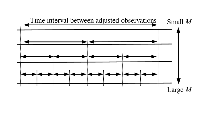
Figure 1: Relationship between $M$ (the number of samples = the number of observations) and time interval. A smaller $M$ results in a longer time interval between adjusted observations.

An important aspect of defining noises from the data generated by a dynamical system is the relationship of number of data with the apparent independence between sample data. This also can be interpreted from the point of correlation time (Fig. 1). Suppose that $x_{ij}$s are generated by some dynamical systems and only $N_{1}$ variables have a sufficiently long correlation time compared with the observation time length. In this case, $j$ is regarded as the time point. How long should the correlation time be to be detected as signals? A smaller $M$ means that the time interval between individual observations is long if we can assume that the observations are performed randomly and uniformly in time at distinct time points. Thus, if the $i$ variables are regarded as signals in the limit of $M=0$, they must have an infinitely long correlation time. This suggests that the deviation rate from the normal distribution as the number of samples decreases varies with the correlation length of the background dynamical system. Since variables with short-term correlations show normal distributions faster as the number of samples decreases, they are regarded to be “noise-like” variables, whereas variables with opposite properties are assumed to be “signal-like” variables.

Thus, our definition of signals is, in some sense, coincident with the order parameter in physics. Thus, in the following, we do not intentionally distinguish a small $M$ from long intervals between observations.

The noise formulation mechanism to distinguish between noises and signals based on the size dependence was successfully applied to various analyses of omics data sets. For example, the method developed by Taguchi and Turky [12] successfully discriminates deferentially expressed genes (signals) from nondifferentially expressed genes (noises) better than several state-of-the-art methods. It was also successfully applied to the identification of differentially methylated cytosine (signals) [13].

The discussion above gives a completely different perspective on the extraction of signals from physics data. To extract signal variables from a variable set, we only need to extract variables whose independence among samples does “not” behave as noise-like as the number of samples decreases. In other words, the extraction of signals does not require the definition of signals. In this paper, we propose a very distinct definition of a signal, that is, a signal is not a noise. To do this, we first define the noise in the next section. In addition to this, we also assume that the signal is always together with a fairly large number of noises and that it can be distinguishable from noises. In this sense, we need noises to define a signal is. Our definition is not useful when only a signal exists. In this paper, $x_{ij}\in\mathbb{R}^{N\times M}$ represents the $j$th measurement of the $i$th variable. $j$ is also regarded to be a time point since each observation must take place at a distinct time point.

In the next section, we define the noise as mentioned above.

II Noise

A noise is defined according to its relationship with other samples. If $x_{ij}$ is independent of all $x_{ij^{\prime}}$ with $j^{\prime}\neq j$, then we define it as a noise, which is definitely an empirical definition. $x_{ij}$ can be a signal even if $x_{ij}$ is independent of all $x_{ij^{\prime}}$ with $j^{\prime}\neq j$. For example, if $x_{ij}$ is only a signal and all $x_{ij^{\prime}}$ with $j^{\prime}\neq j$ are random numbers, $x_{ij}$ is independent of all $x_{ij^{\prime}}$ with $j^{\prime}\neq j$, but it is still a signal. However, if $x_{ij}$ is a noise, it is definitely independent of all $x_{ij^{\prime}}$ with $j^{\prime}\neq j$. Therefore, it is only a sufficient condition for noises. However, we start from here and see what is going on.

Next, we define how to decide which variables are independent of others. We can use the correlation coefficients $\rho_{ii^{\prime}}$ between variables as

$$\rho_{ii^{\prime}} = \frac{\sum_{j}\left(x_{ij}-\langle x_{ij}\rangle\right)\left(x_{i^{\prime}j}-\langle x_{i^{\prime}j}\rangle\right)}{\sqrt{\sum_{j}\left(x_{ij}-\langle x_{ij}\rangle\right)^{2}}\sqrt{\sum_{j}\left(x_{i^{\prime}j}-\langle x_{i^{\prime}j}\rangle\right)^{2}}}$$ (2)

$$\langle x_{ij}\rangle = \frac{1}{M}\sum_{j}x_{ij}$$ (3)

$$\langle x_{i^{\prime}j}\rangle = \frac{1}{M}\sum_{j}x_{i^{\prime}j}.$$ (4)

However, they are unlikely to be useful since we cannot determine the boundary between noise and signal from the value of $\rho_{ii^{\prime}}$.

Alternatively, we can use the joint probability

$$P(x_{ij},x_{i^{\prime}j})=P(x_{ij})P(x_{i^{\prime}j})$$ (5)

as a condition of independence between $i$ and $i^{\prime}$ [14]. It is an acceptable idea, but it has some limitations; we need a large $M$ to accurately estimate $P$. As can be seen below, we need to consider the cases with a small $M$. Actually, we will make use of the smallness of $M$ to define what a signal is. Thus, these ideas are also useless to us.

Instead of these conventional approaches, we will do the following: First, we apply the singular value decomposition (SVD) [2] to $x_{ij}$ as

$$x_{ij}=\sum_{\ell}\lambda_{\ell}u_{\ell i}v_{\ell j},$$ (6)

and we attribute $P$ values to $u_{\ell i}$ assuming the null hypothesis that $u_{\ell i}$ obeys a Gaussian distribution:

$$P_{i}=P_{\chi^{2}}\left[>\left(\frac{u_{\ell i}}{\sigma_{\ell}}\right)^{2}\right],$$ (7)

where $P_{\chi^{2}}[>x]$ is the cumulative $\chi^{2}$ distribution where the argument is larger than $x$ (Appendix D) and $\sigma_{\ell}$ is the optimal standard deviation chosen so that $u_{\ell i}$ obeys a Gaussian distribution as much as possible [12] (see Appendix A and above). We empirically assume that $\sum_{i}x_{ij}=0$ in the above. If not, it should be so during preprocessing. If $P_{i}$ is not sufficiently small (i.e., not significant) after the multiple correlation correction (see below), we consider that the variable $i$ is a noise. In which sense is the $i$th variable a noise? This can be understood if one can see the corresponding $v_{\ell j}$ that represents the signal.

The underlying assumption of the above is as follows. If all $x_{ij}$ are random, all $u_{\ell i}$ obey a Gaussian distribution. Thus, no matter what $v_{\ell j}$s are, all $i$ variables are noises. However, if some $i$s (without loosing generality, we assume that there are $N_{1}$ variables supposed to be signals and they are re-ordered so as to be top $i\leq N_{1}$) are signals in the sense that $v_{\ell j}$s are signals, the corresponding $u_{\ell i}$s should be outliers under the Gaussian distribution, since the summation of $N_{1}$ signals increases with the order of $N_{1}$, whereas the amplification by the summation of other noises is at most $\sqrt{N-N_{1}}$. In addition to this, a larger $M$ enables us to detect “signality”, which represents how more likely variables are regarded as signals, more easily, since even if they are marginally to be signals, noises hardly correlate with one another at larger $M$ values. In contrast, if $i$th variables can be detected as signals for smaller $M$ values, this suggests that variables $i$s are more likely signals. In this sense, we define the signals as those identified to be signals even if $M$ becomes zero ($M=0$ limit).

III Empirical procedures for detecting signals

Although the above idea might be reasonable, we have to be more quantitative in order to detect signals in real situations. To realize this, we carry out the following. First, we need to find which $v_{\ell j}$ can be regarded as signals. In this sense, our definition of signals is subjective. However, one should remember that $v_{\ell j}$s are generated in a fully data-driven manner. If one cannot find any $v_{\ell j}$ that are likely to be signals, one can consider that there are only noises. This is empirically not a problem, since the number of distinct $v_{\ell j}$ is limited by $M$ and we consider the case of $M=0$ limit; therefore, the number of $v_{\ell j}$ that we have to investigate should be very limited.

Next, we need to estimate the standard deviation (SD) used for the inference of the Gaussian distribution (or the attribution of $P$ values to $i$’s). The estimation is not straightforward since we have to exclude $i$s that can be regarded to be signals; otherwise, SD is overestimated, which results in larger (thus less significant) $P$-values. If we successfully exclude $i$s to be signals and can estimate the SD coincident with the Gaussian distribution that noises obey, the histogram of $P_{i}$, i.e., $h_{n}$ representing the number of $i$s that belong to the $n$th bin should be flat. Thus, if we draw $h_{n}$ (for conventional reasons, $1-P_{i}$ is often considered not $P_{i}$), it is flat (Appendix E) excluding the sharp peak at $1-P_{i}\sim 1$ (i.e., $P_{i}\sim 0$, see Fig. 2).

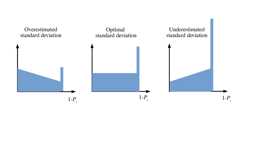
Figure 2: The shape of the histogram of $1-P_{i}$ can vary with the estimated SD.

If SD is overestimated, $h_{n}$ for a smaller $1-P_{i}$ is increased. If SD is underestimated, $h_{n}$ for a larger $1-P_{i}$ is increased (Fig. 2). Thus, to have an optimal SD, we can minimize the SD of $h_{n}$ for $n<n_{0}$, where $n_{0}$ is the smallest bin that includes outliers. As can be seen below, this empirical definition of SD practically works well.

After addressing $P_{i}$s to $i$s, $P_{i}$s are corrected by multiple comparison corrections (e.g., the Benjamini-Hochberg (BH) criterion) and $i$s associated with adjusted $P_{i}$ less than the threshold value, $P_{0}$ ($P_{0}$ is typically taken to be 0.05 or 0.01) are selected. This is the proposed method of distinguishing signals from noises. We examine which variables $i$s are selected as signals with $M$ changed by the random sampling of $M_{\mbox{res}}(\leq M)$ $j$s, and we define signals when $M_{\mbox{res}}$ is selected to be very small (taking $M_{\mbox{res}}=0$ limit might be unrealistic in the real situations). This was implemented as two of the Bioconductor Packages [15, 16] and is freely available.

IV Real Examples

We consider two types of data set to demonstrate the effectiveness of our framework, i.e., datasets generated from the globally coupled map [17] (GCM) and those generated in genomic science.

IV.1 GCM

To generate variables that are a mixture of ordered and random states, we introduce GCM with random parameters as

$$x_{ij+1} = g_{ii}f(x_{ij},a_{i})+\frac{1}{N}\sum_{i^{\prime}=1}^{N}g_{ii^{\prime}}f(x_{i^{\prime}j},a_{i^{\prime}})$$ (8)

$$g_{ii^{\prime}} = (1-c)\delta_{ii^{\prime}}+c\epsilon_{ii^{\prime}}$$ (9)

$$a_{i} = a+(1-a)\epsilon_{i}$$ (10)

$$f(x,a) = 1-ax^{2}$$ (11)

where $\epsilon_{ii^{\prime}}$ and $\epsilon_{i}$ are uniform random numbers as $\epsilon_{i},\epsilon_{ii^{\prime}}\sim[0,1]$. $a=1.75,c=0.04,$ and $N=10^{4}$ in this study such that a single $f[x,a]$ falls in the chaotic region ($a>1.48$). $c$, which expresses the strength of the pairwise interaction between individual maps, is taken to be sufficiently small not to suppress the chaotic nature completely because of synchronization among individual maps, $f(x,a)$ to have the mixture of ordered and random states. $j$s are taken to be $1\leq j\leq 10^{2}$. Thus, the generated dataset is $x_{ij}\in\mathbb{R}^{10^{4}\times 10^{2}}$. Initial values ($x_{i0}$) are drawn from the same uniform distribution, $[0,1]$.

IV.2 Genomics data

Since this framework was originally proposed for processing genomic data [18], we demonstrated the effectiveness of this framework using genomic data sets, retrieved from The Cancer Genome Atlas (TCGA).

IV.2.1 Methylation profiles

The data of the methylation profile recovered from TCGA are $x_{ij}\in\mathbb{R}^{48557\times 895}$ (for more details, see Breast data from TCGA [13]). They are associated with the labels shown in Table 1.

Labels	none	3rd	4th	5th	6th	7th
Frequency	102	3	18	72	277	422

Table 1: Frequency of labels associated with methylation data.

IV.2.2 Gene expression profiles

The data of gene expression profile recovered from TCGA are $x_{ij}\in\mathbb{R}^{20532\times 1020}$. They are KIPAN.rnaseq in RTCGA.rnaseq, and “patient.stage_event.pathologic_stage” from RTCGA.clinical is used as the classification label (for more details, see [19]).

IV.3 Evaluation of features

To determine if individual features remain non-Gaussian as the sample number decreases, we re-sample $M_{\mbox{res}}$ samples from $M$ samples and attribute $P$-values to individual features, $i$. $P$-values are corrected on the basis of the BH criterion [18], and $i$s associated with the adjusted $P$-values less than the threshold values are selected. Re-sampling is repeated one hundred times (one thousand times for regression analysis leading to eq. (23) shown later), and we count the frequency of individual $i$s selected as non-Gaussian (i.e., those associated with the adjusted $P$-values less than the threshold values). $h_{\max}$ is the number of features selected as signals by more than 9950 (for gene expression) times among one thousand trials where the threshold $P$-value is taken to be 0.01. For GCM, $\langle n_{i}\rangle_{300}$, whose defintion is described in the text, is used instead of $h_{\mbox{max}}$.

V Results

V.1 GCM

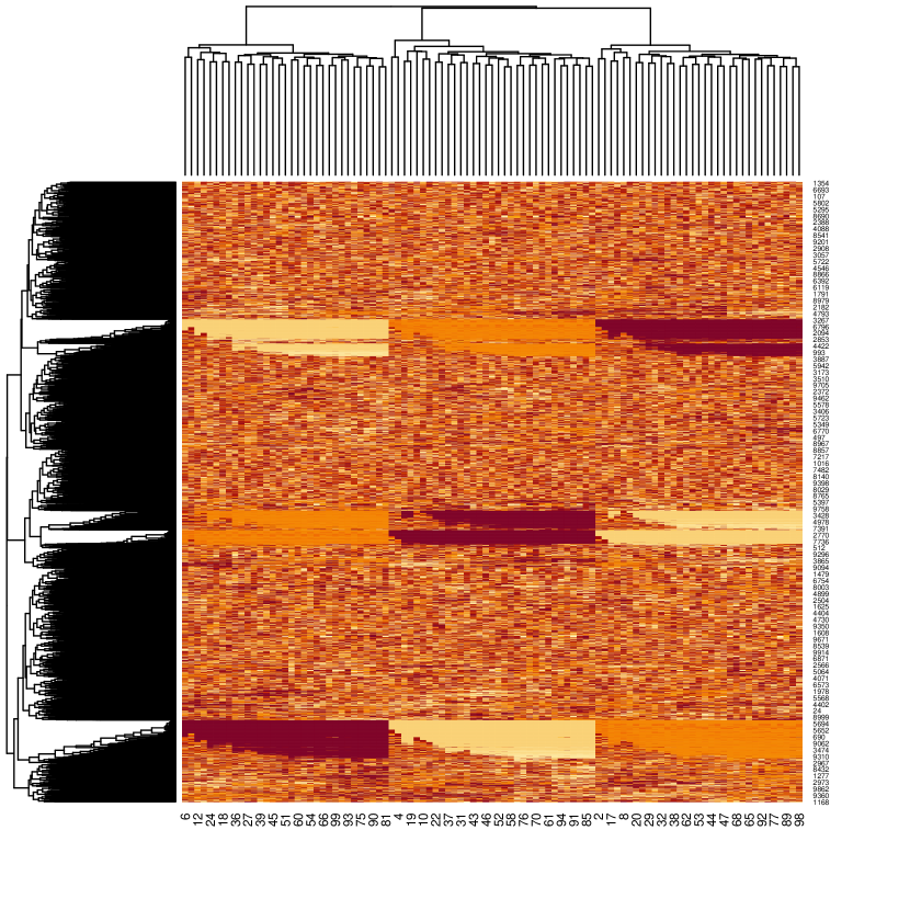
Figure 3: Heatmap of $x_{ij}\in\mathbb{R}^{10^{4}\times 10^{2}}$ generated using GCM.

Figure 3 shows the heatmap of $x_{ij}\in\mathbb{R}^{10^{4}\times 10^{2}}$ generated using GCM. It is obvious that the obtained states using GCM are a mixture of a large number of random variables and a small number of synchronized three-state variables that have a long correlation time and are supposed to be regarded as signals. The purpose of the analysis is to identify the three state variables as signals. From GCM data, we do not select $v_{\ell j}$ coincident with classification labels every time we re-sample, but we always employ the first one, $v_{1j}$, and the corresponding $u_{1j}$ for feature selection. SD was not optimized either and $\sigma_{1}$ is fixed to be $1\times 10^{-3}$.

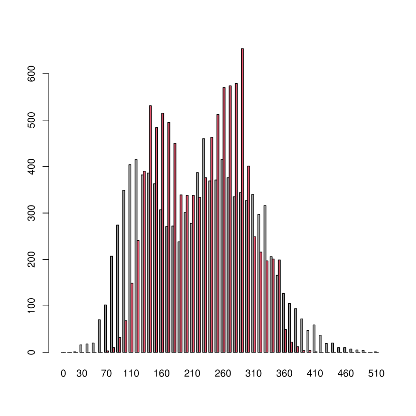
Figure 4: Histogram of the frequency to be regarded as non-Gaussian of individual features (GCM), $i$. Red, $M_{\mbox{res}}=8$; Grey, $M_{\mbox{res}}=14$. The threshold $P$-value is 0.05 and the number of trials (re-sampling) is one thousand.

After all trials (one hundred times or one thousand times) finished, the frequency of being selected were computed for all $N$ features. Figure 4 shows the histogram (vertical axis) of the frequency (horizontal axis) to be considered as non-Gaussian of individual features (GCM), i.e., $i$ for $M_{\mbox{res}}=8$ and $14$ (see Appendix C for more deailed procedure). As one can see, the number of features regarded as non-Gaussian decreases as the number of samples, $M_{\mbox{res}}$, decreases.

V.2 Genomic data

V.2.1 DNA methylation

Figure 5 shows the typical $v_{\ell j}$ associated with the class labels (Table 1). This is the “signal” defined in this study since it is coincident with the class labels, and is obtained in a fully data-driven manner (see Appendix C for more detailed procedures to obtain this plot)

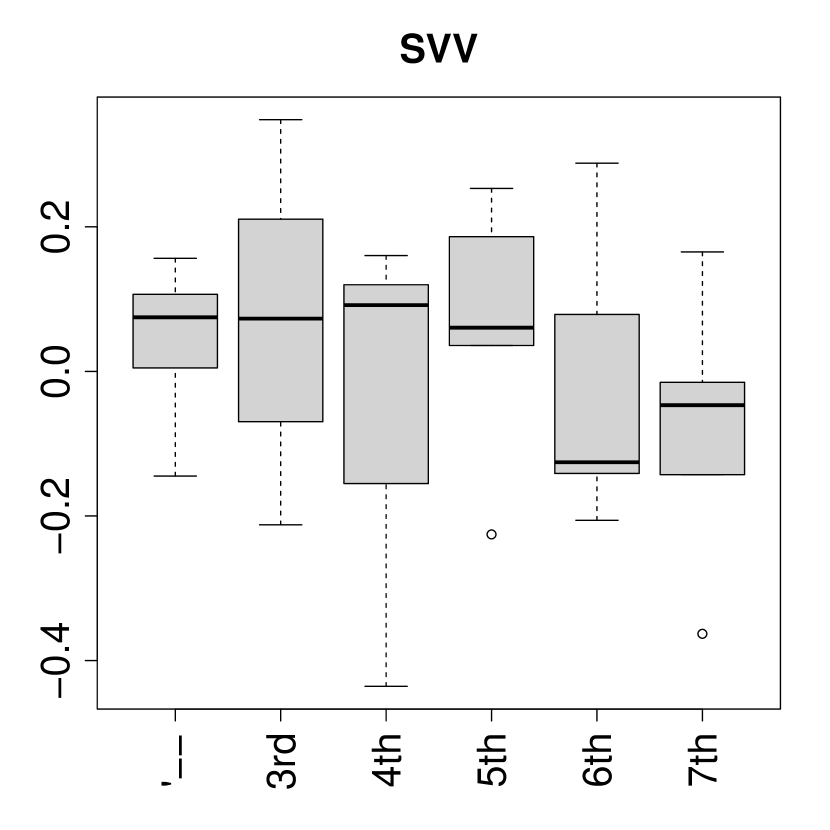
Figure 5: Typical example of boxplot of $v_{\ell j}$ associated with the smallest $P$-value ($P=0.03$) for methylation data set when $M_{\mbox{res}}=28$.

This is only the fifteenth SVV; thus, it is associated with a very small amount of contribution. $P$-values are attributed to the $i$th features obtained using eq. (7) with the optimized $\sigma_{\ell}$ so that the corresponding $u_{\ell i}$ obeys the Gaussian distribution as much as possible (see Appendix 15 for the optimization of $\sigma_{\ell}$).

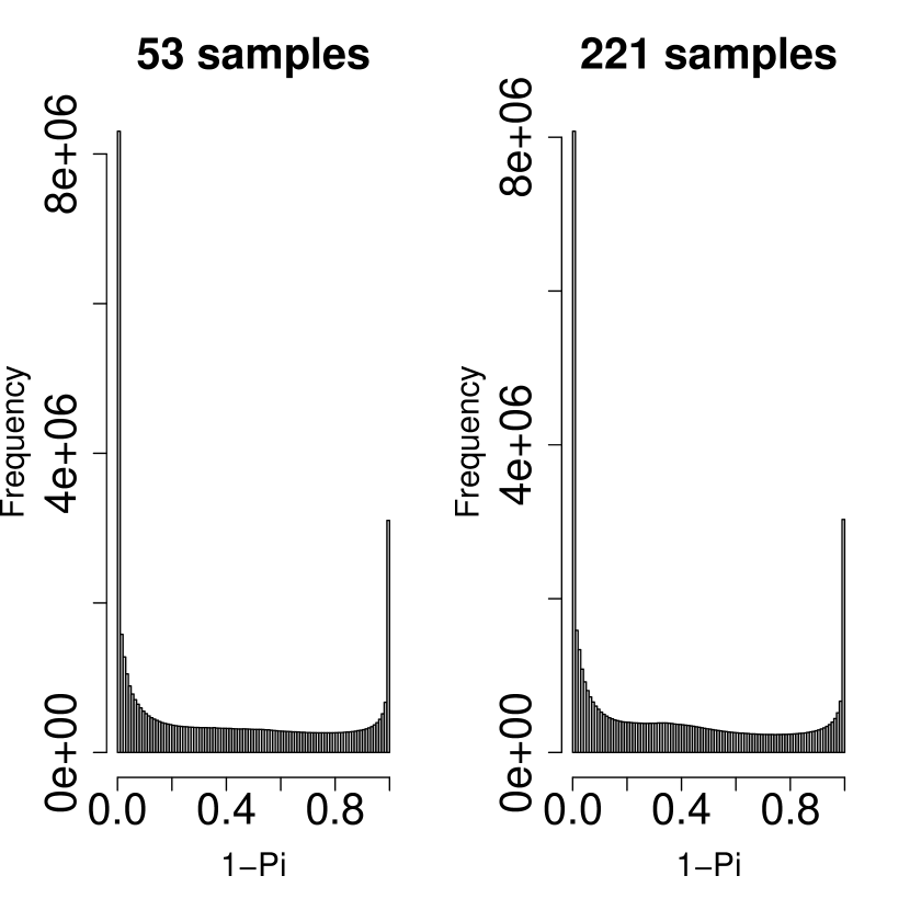
Figure 6: Histogram of $1-P_{i}$ after re-sampling in one hundred trials. Left, $M_{\mbox{res}}=53$; right, $M_{\mbox{res}}=221$.

Figure 6 shows the histogram of $1-P_{i}$. As expected, the histogram is almost flat excluding the sharp peak at $1-P_{i}\simeq 1$ (i.e., $P_{i}\simeq 0$). On the other hand, the peak at $P_{i}\simeq 1$ corresponds to sites without methylation at all regardless of the class labels; thus, there are no reasons for features to be coincident with class labels and can be ignored.

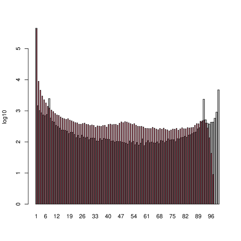
Figure 7: Logarithmic histogram of the frequency to be regarded non-Gaussian of individual features (methylation sites), $i$. Red, $M_{\mbox{res}}=53$; Grey, $M_{\mbox{res}}=221$. The threshold $P$-value is 0.01 and the number of trials (re-sampling) is one hundred.

From Fig. 6, we counted the frequency of association of features, $i$s, with adjusted $P$-values less than the threshold value of 0.01 (see subsection IV.3 for more detailed procedures), which means that the features obey non-Gaussian, i.e., they are signal variables. Figure 7 shows the histogram (vertical axis) of the frequency (horizontal axis) to be considered non-Gaussian of individual features (methylation sites), $i$ for $M_{\mbox{res}}=53$ and $221$. As one can see, there are no features selected as non-Gaussian with 100% probability for $M_{\mbox{res}}=53$, whereas there are some features selected for $M_{\mbox{res}}=221$. This suggests that our framework indicates that the number of features regarded as non-Gaussian will decrease as the number of samples, $M_{\mbox{res}}$, decreases. On the other hand, since there are no features regarded as non-Gaussian for $M_{\mbox{res}}=53$, one might wonder if there are any signal features when $M_{\mbox{res}}=0$ limit. Although the expectation that the number of features regarded as signals will decrease as $M_{\mbox{res}}$ decreases is fulfilled, it is unlikely that some features remain as signals in the limit of $M_{\mbox{res}}=0$.

V.2.2 Gene expression

Since DNA methylation has no signal variables in the limit of $M_{\mbox{res}}=0$, we consider yet another feature, the gene expression profile. Since the processes until we obtain the histogram of frequency to be selected as signals among one hundred trials do not change markedly, we decided to skip these processes since they are not essential.

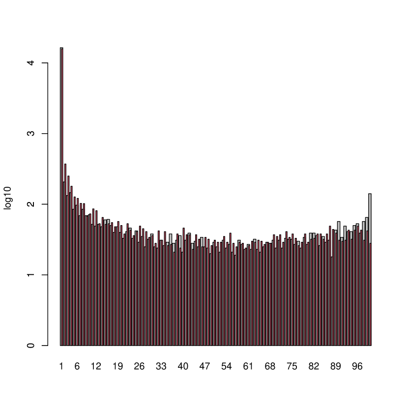
Figure 8: Logarithmic histogram of the frequency to be regarded non-Gaussian of individual features (gene expression), $i$. Red, $M_{\mbox{res}}=20$; Grey, $M_{\mbox{res}}=40$. The threshold $P$-value is 0.01 and the number of trials (re-sampling) is one hundred.

Figure 8 shows the histogram (vertical axis) of the frequency (horizontal axis) to be considered non-Gaussian of individual features (gene expression), $i$ for $M_{\mbox{res}}=20$ and $40$, respectively. As one can see, there are some features selected as non-Gaussian with 100% probability even for $M_{\mbox{res}}=20$ in contrast to the methylation case, although the number of features regarded as non-Gaussian will decrease as the number of samples, $M_{\mbox{res}}$, decreases (see Discussion on this point). Thus, our framework seems to be applicable to not only numerical models such as GCM but also genomic data.

VI Discussion

As for the equivalence between correlation time and sample size, we can be more quantitative since we have discussed equivalence in some specific examples. In GCM, the situation is a mixture of random and ordered stats. Suppose the random state has the finite correlation time $\tau$, the probability that two time points are separated by the time interval $T$ will decrease as

$$P\sim\exp\left(-\frac{t}{\tau}\right)$$ (12)

and, as discussed in the above $t\sim\frac{1}{M}$ (Fig. 1),

$$P\sim\exp\left(-\frac{1}{M\tau}\right).$$ (13)

Thus, an ordered state can be detected if two time points maintain the same number of values compared with the probability $P$. Since $M=0$ limit, i.e., $P=1$, only true (perfect) ordered state can have probability larger than $P$ defined above. In genomic data, random (uncorrelated) genes are assumed to obey Gaussian and the probability that they have finite values is

$$P\sim\exp\left(-\frac{x^{2}}{2\sigma^{2}}\right)$$ (14)

and $\sigma\sim\sqrt{M}$; then,

$$P\sim\exp\left(-\frac{x^{2}}{M}\right).$$ (15)

Genes associated with $x$ values with a sufficiently small $P$ defined above are considered highly expressed. In this sense, in the current data sets, namely, genomic data and GCM, the number of features selected as those associated with a sufficiently small $P$ is expected to have the same dependence on $M$ and can be treated in the same framework proposed here.

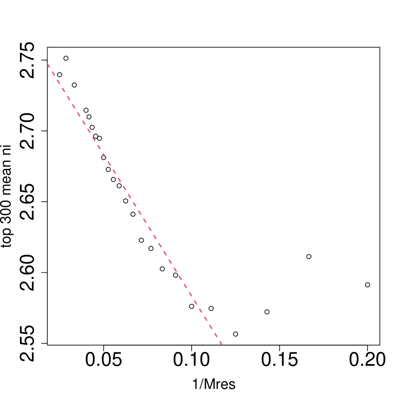
Figure 9: Scatter plots of top 300 mean $n_{i}$, $\langle n_{i}\rangle_{300}$, vs $M_{\mbox{res}}$ for GCM ($M_{\mbox{res}}=5,\cdots,25,30,35,40$). Vertical, $\log(\langle n_{i}\rangle_{300})$; horizontal, $\frac{1}{M_{\mbox{res}}}$. The red broken line is the regression line for $8\leq M_{\mbox{res}}\leq 30$.

There are some possibilities to evaluate $P$ in the above equations. For GCM, we performed the following; Suppose that $n_{i}$ is the occurrence of association of features with the adjusted $P$-values less than the threshold values in one hundred or one thousand trials. Then, we averaged $n_{i}$ for the top 300 features ranked and denoted it as $\langle n_{i}\rangle_{300}$. As the possibility $P$ in the above equations decreases, $\langle n_{i}\rangle_{300}$ is also expected to decrease. Figure 9 shows the dependence of $\langle n_{i}\rangle_{300}$ on $M_{\mbox{res}}$ in one thousand trials in Fig. 4. As expected,

$$\log\langle n_{i}\rangle_{300}=a-\frac{b}{M_{\mbox{res}}},$$ (16)

where $a$ and $b$ are the regression coefficients optimized by linear regression [20].

For gene expression, we evaluate $P$ in a different manner, since some features remain associated with the adjusted $P$-values less than the threshold values with 100% probability in $M_{\mbox{res}}=0$ limit (Fig. 8). For the evaluation of $P$, we employ $h_{\max}$ in the histogram of $1-P_{i}$ in the highest $1-P_{i}$ bin (i.e., the height of the rightmost bin in Fig. 8). Then, we expect

$$\log h_{\max}=a-\frac{b}{M_{\mbox{res}}},$$ (17)

where $a$ and $b$ are the regression coefficients optimized by linear regression [20].

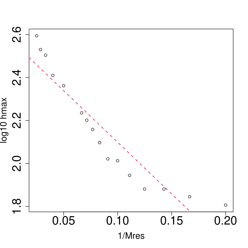
Figure 10: Scatter plots of histogram in the highest bin, $h_{\max}$, vs $M_{\mbox{res}}$ for gene expression ($M_{\mbox{res}}=5,6,\cdots,15,20,25,30,35,40$). Vertical, $\log(h_{\max})$; horizontal, $\frac{1}{M_{\mbox{res}}}$. The red broken line is the regression line.

Figure 10 shows the dependence of $h_{\max}$, on $M_{\mbox{res}}$. As expected, since $\log h_{\max}$ decreases roughly proportionally to $\frac{1}{M_{\mbox{res}}}$, our postulate, “Signals can be defined as features that remain non-Gaussian even when the sample size is equal to the zero limit,” seems to be correct.

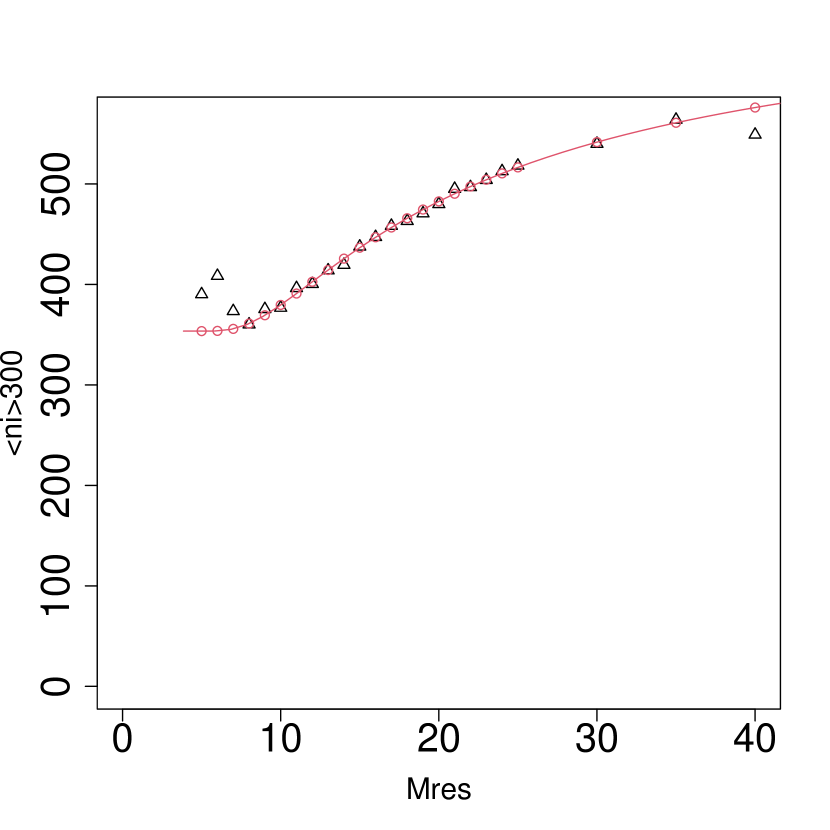
Figure 11: Fitting result of data shown in Fig. 9 (black open triangles) with eq. (18) (red curve and open red circles only for $8\leq M_{\mbox{res}}\leq 30$; the actual regression equation is not eq. (18) but eq. (20)). $n_{0}=353.57,\alpha=5.84,\beta=15.8,$ and $M_{\mbox{lim}}=3.85$.

In a more advanced fitting for GCM,

$$\langle n_{i}\rangle_{300}=n_{0}+\alpha\exp\left(-\frac{\beta}{M_{\mbox{res}}-M_{\mbox{lim}}}\right),$$ (18)

which is equivalent to

$$\log\left(\langle n_{i}\rangle_{300}-n_{0}\right) = \log\alpha-\frac{\beta}{M_{\mbox{res}}-M_{\mbox{lim}}}$$ (19)

$$M_{\mbox{res}} = M_{\mbox{lim}}-\frac{\beta}{\log\left(\langle n_{i}\rangle_{300}-n_{0}\right)-\log\alpha}.$$ (20)

$n_{0}$ is the mean occurrence of the top 300 features when $M_{\mbox{res}}\rightarrow M_{\mbox{lim}}$ (as denoted above, $M_{\mbox{res}}=0$ is unrealistic in a real data set). Nonlinear regression [21] is performed for eq. 20. Since the fitting is relatively good (Fig. 11), our postulate seems to be correct.

Empirically, the same discussion is expected to be also effective for gene expression, since the dependence of how to select features on $M$ is common between eqs. (14) and (15). Then we propose

$$h_{\max}=h_{0}+\alpha\exp\left(-\frac{\beta}{M_{\mbox{res}}-M_{\mbox{lim}}}\right)$$ (21)

which is equivalent to

$$\log\left(h_{\max}-h_{0}\right) = \log\alpha-\frac{\beta}{M_{\mbox{res}}-M_{\mbox{lim}}}$$ (22)

$$M_{\mbox{res}} = M_{\mbox{lim}}-\frac{\beta}{\log\left(h_{\max}-h_{0}\right)-\log\alpha}$$ (23)

In actual situations, $\log h_{\max}$ also decreases roughly proportionally to $\frac{1}{M_{\mbox{res}}}$ (Fig.10). As can be seen in Fig. 12, the nonlinear fitting [21] for eq. (21) is relatively good for gene expression data as well. Thus, our postulate, “Signals can be defined as features that remain non-Gaussian even when the sample size is equal to the zero limit,” seems to be effective for not only numerical models (GCM) but also real data sets (gene expression).

To date, we have not known why our framework, PCA or TD-based unsupervised FE, works very well especially when there are a small number of samples associated with many variables. In this study, smaller-size samples have advantages in the identification of ordered state variables with a long correlation time. Although there is no explicitly defined time progression in gene expression profiles, they also should be generated by a certain dynamical system (possibly, the so-called gene regulatory network). If so, it is not surprising at all that our framework has advantages in the detection of signals (ordered state) particularly when there are only a small number of samples, since a small-size sample limit might correspond to a long-time limit (Fig. 1) where only the truly ordered state with an infinitely long correlation time can survive. In this sense, gene expression profiles coincident with some classification labels correspond to the ordered state generated by underlying dynamical systems.

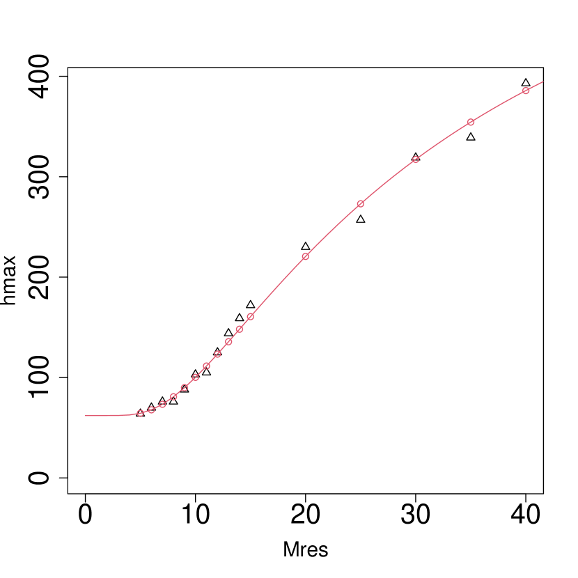
Figure 12: Fitting result of the data shown in Fig. 10 (black open triangles) with eq. (21) (red curve and open red circles represent the regression curve and estimated values at corresponding data points, and the actual regression equation is not eq. (21) but eq. (23)) . $h_{0}=62.2,\alpha=6.49,\beta=28.6$, and $M_{\mbox{lim}}=0$.

Finally, we investigated how our framework can capture signal features in more detail for GCM.

Figure 13: $v_{1j}$ used as a template of “signal” in this study.

As described above, what we have done is to find features coincident with $v_{\ell j}$, where $\ell=1$ was employed for GCM in this study. On the other hand, the purpose of this analysis is to select three state variables shown in Fig. 3. Figure 13 shows $v_{1j}$, which does not appear smilar to the three states at all.

Figure 14: Heatmap of $x_{ij}$ associated with top 1200 $n_{i}$ averaged over one thousand trials.

Despite this, the features associated with the top 1200 $n_{i}$s (the threshold $P$-values are set to be 0.01) averaged over one thousand trials for $M_{\mbox{res}}=8$ are enriched with three state variables (Fig. 14). This definitely demonstrates the effectiveness of our framework. No subjective criterion can likely identify $v_{1j}$ as signals. Nevertheless, the features associated with $v_{1j}$ are also well associated with three state variables (Fig. 14). In this sense, our new framework for identifying “signals” as those distinct from “noises” defines “signals” as those that do not obey Gaussian; this definition is distinct from the usual definition of “signals”, but effective.

Appendix A Optimization of SD

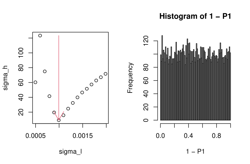
Figure 15: Demonstration of optimization of $\sigma_{h}$ for pure Gaussian. Left: dependence of $\sigma_{h}$ on $\sigma_{\ell}$. Right: histogram of $1-P_{i}$ with optimized $\sigma_{\ell}$.

1. Set the initial $\sigma_{\ell}$.

2. Compute $P_{i}$ with eq. (7).

3. Compute histogram $h_{n}$ of $1-P_{i}$, where $h_{n}$ is the number of $i$s that satisfy $\frac{n-1}{N_{h}}<1-P_{i}\leq\frac{n}{N_{h}}$. $N_{h}$ is the number of bins. Typically, $N_{h}=100$.

4. Compute the adjusted $P_{i}$ considering multiple comparison corrections (e.g., BH criterion).

5. Exclude the count of $i$ with the adjusted $P_{i}$ less than the threshold value $P_{0}$ (typically, $P_{0}=0.01$ or $0.05$).

6. Compute the SD of $h_{n}$, $\sigma_{h}$, as

   $$\sigma_{h} = \sqrt{\frac{1}{N_{h}}\sum_{n}\left(h_{n}-\langle h_{n}\rangle\right)^{2}}$$ (24)

   $$\langle h_{n}\rangle = \frac{1}{N_{h}}\sum_{n}h_{n}.$$ (25)

7. Find $\sigma_{\ell}$ with the smallest $\sigma_{h}$.

Figure 15 shows the demonstration of the above procedure applied to ten thousand random features that obey Gaussian with zero mean and SD ($\sigma_{\ell}$) of $1\times 10^{-3}$. As expected, $\sigma_{\ell}=1\times 10^{-3}$ is associated with the minimum $\sigma_{h}$.

Appendix B Regression analysis

Regression analysis for eq. (23) was performed using the nls function in R in the form

$$M_{\mbox{res}}\sim M_{\mbox{lim}}-\frac{\beta}{\log\left(h_{\max}-h_{0}\right)-\log\alpha},$$ (26)

i.e., $M_{\mbox{res}}$ is regarded as the dependent variable and $h_{\max}$ the independent variable, whereas $M_{\mbox{lim}},\alpha,\beta$, and $h_{0}$ are regarded as regression coefficients. Lower bounds for $M_{\mbox{lim}}$ and $h_{0}$ are set to be equal to zero and the upper bound of $h_{0}$ is set to be $\min(h_{\max})$ to avoid the argument of $\log\left(h_{\max}-h_{0}\right)$ becoming negative. In addition to this, the algorithm=“port” option is used to make the upper and lower bounds effective.

For GCM (i.e., eq. (20)), the above is performed with replacing $h_{\max}$ and $h_{0}$ with $\langle n_{i}\rangle_{300}$ and $n_{0}$, respectively.

Appendix C Detailed procedure of re-sampling

After re-sampling, we have $x_{ij}\in\mathbb{R}^{N\times M_{\mbox{res}}}$ to which SVD was applied. Categorical regression is applied to obtain $v_{\ell j}$ as

$$v_{\ell j}=a_{\ell}+\sum_{s}b_{\ell s}\delta_{sj},$$ (27)

where $\delta_{sj}$ takes 1 when the $j$th sample belongs to the $s$th category, otherwise 0. The above categorical regression was performed with the lm function implemented in R. $\ell$ associated with the smallest $P$-value was selected and $\sigma_{\ell}$ was optimized toward $u_{\ell i}$ as described in Appendix 15. $P$-values were attributed to $i$th as in eq. (7) and corrected with the BH criterion, and the features associated with the adjusted $P$-values less than the threshold values (0.01 or 0.05) were selected. After all the trials (one hundred or one thousand times) were completed, the frequency of a feature being selected was computed for all $N$ features. Then, $h_{\max}$ was determined as described in §IV.3.

Appendix D Explanation of eq. (7)

Since the majority of physicists who consist of majority reading this journal might not be very familiar with eq. (7), we briefly outline the reasoning for eq. (7). $P_{\chi^{2}}$ is generally equivalent to the probability of the occurrence of events in which random workers who start at the origin go beyond some distance far from the origin. Suppose that $u_{\ell}$ is the one-step distance for the $\ell$th step and $u_{\ell}$ is supposed to obey the Gaussian distance of zero mean and the standard deviation of $\sigma_{\ell}$. Then, the squares of the distance of the worker at the $L$th step from the origin obey the probability

$$P_{\chi^{2}}\left[>\sum_{\ell=1}^{L}\left(\frac{u_{\ell}}{\sigma_{\ell}}\right)^{2}\right].$$ (28)

When the squares of the distance of the worker are too large to occur under the Gaussian distribution, we can regard the null hypothesis that $u_{\ell}$ obeys the Gaussian as presumably wrong. Usually, the $\chi^{2}$ test obeying the above $P$ distribution is used for the evaluation of independence between $u_{\ell}$s, and we used this test inversely; i.e., if $u_{\ell}$s could not pass this test, we regarded them as non-Gaussian, i.e., signal variables under the context of this study.

Appendix E Explanation of flatness of the histogram of $P$-values [22]

Here is a brief explanation of why the histogram of the $P$-values computed using eq. (7) must be flat, as can be seen in Fig. 15, if the null hypothesis that $u_{\ell i}$ obeys Gaussian is correct. Actually, it is not a field-specific truth, but a consequence of the fact when events occur probabilistically.

Suppose that some random variable $x$ obeys the distribution of $P(x)$, but we do not know $P(x)$ and wrongly assume that $x$ obeys $Q(x)\neq P(x)$. Then, we attribute $P$-values to $x$ using $Q(x)$. Because of the identity

$$\int dP=P,$$ (29)

the histogram of $P$ should then always be flat (Fig. 16). However, if we wrongly compute the left-hand side by counting the number of $P$-values computed using $Q$, this generally does not stand, i.e.,

$$\int dQ\neq Q.$$ (30)

Thus, by determining if the histogram of $P$-values is flat, we can evaluate if $Q=P$ (i.e., the correctness of $Q$) or not.

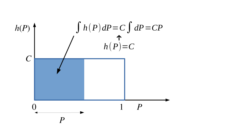
Figure 16: Shaded area is equal to $\int h(P)dP$. When $h(P)$ takes a constant value, $C$, $\int h(P)dP=CP$. Since $\int dP=P$ is identity, $h(P)$ must be constant if $P$ is correctly attributed, e.g., by using the distribution function that generates random variables.

References

- Vitányi [2011] P. M. B. Vitányi, On empirical entropy, CoRR abs/1103.5985 (2011), 1103.5985 .
- Hastie et al. [2009] T. Hastie, R. Tibshirani, and J. Friedman, The elements of statistical learning: data mining, inference and prediction, 2nd ed. (Springer, 2009).
- Ho et al. [2020] J. Ho, A. Jain, and P. Abbeel, Denoising diffusion probabilistic models, in Advances in Neural Information Processing Systems, Vol. 33, edited by H. Larochelle, M. Ranzato, R. Hadsell, M. Balcan, and H. Lin (Curran Associates, Inc., 2020) pp. 6840–6851.
- Cayton [2005] L. Cayton, Algorithms for manifold learning, Univ. of California at San Diego Tech. Rep 12, 1 (2005).
- Narayanan and Mitter [2010] H. Narayanan and S. Mitter, Sample complexity of testing the manifold hypothesis, Advances in neural information processing systems 23 (2010).
- Rifai et al. [2011] S. Rifai, Y. N. Dauphin, P. Vincent, Y. Bengio, and X. Muller, The manifold tangent classifier, Advances in neural information processing systems 24 (2011).
- Bengio et al. [2013] Y. Bengio, A. Courville, and P. Vincent, Representation learning: A review and new perspectives, IEEE transactions on pattern analysis and machine intelligence 35, 1798 (2013).
- Mototake and Ikegami [2015] Y. Mototake and T. Ikegami, The dynamics of deep neural networks, in Proceedings of the Twentieth International Symposium on Artificial Life and Robotics, Vol. 20 (2015).
- Vicsek and Zafeiris [2012] T. Vicsek and A. Zafeiris, Collective motion, Physics reports 517, 71 (2012).
- Ikegami et al. [2017] T. Ikegami, Y.-i. Mototake, S. Kobori, M. Oka, and Y. Hashimoto, Life as an emergent phenomenon: studies from a large-scale boid simulation and web data, Philosophical transactions of the royal society a: Mathematical, physical and engineering sciences 375, 20160351 (2017).
- Kawakatsu [2004] T. Kawakatsu, Statistical physics of polymers: an introduction (Springer Science & Business Media, 2004).
- Taguchi and Turki [2022] Y.-h. Taguchi and T. Turki, A tensor decomposition-based integrated analysis applicable to multiple gene expression profiles without sample matching, Scientific Reports 12, 21242 (2022).
- Taguchi and Turki [2023a] Y.-H. Taguchi and T. Turki, Principal component analysis- and tensor decomposition-based unsupervised feature extraction to select more suitable differentially methylated cytosines: Optimization of standard deviation versus state-of-the-art methods, Genomics 115, 110577 (2023a).
- Linton [2017] O. Linton, Probability, Statistics and Econometrics (Academic Press, San Diego, CA, 2017).
- Y-h. Taguchi [2023a] Y-h. Taguchi , TDbasedUFE, https://doi.org/10.18129/B9.bioc.TDbasedUFE (2023a).
- Y-h. Taguchi [2023b] Y-h. Taguchi , TDbasedUFEadv, https://doi.org/10.18129/B9.bioc.TDbasedUFEadv (2023b).
- Kaneko [1990] K. Kaneko, Globally coupled chaos violates the law of large numbers but not the central-limit theorem, Phys. Rev. Lett. 65, 1391 (1990).
- Taguchi [2020] Y.-H. Taguchi, Unsupervised Feature Extraction Applied to Bioinformatics (Springer International Publishing, 2020).
- Taguchi and Turki [2023b] Y.-h. Taguchi and T. Turki, Advanced tensor decomposition-based integrated analysis of protein-protein interaction with cancer gene expression can improve coincidence with clinical labels, bioRxiv 10.1101/2023.02.26.530076 (2023b), https://www.biorxiv.org/content/early/2023/02/27/2023.02.26.530076.full.pdf .
- Chambers and Hastie [1992] J. Chambers and T. Hastie, Statistical models in S, Wadsworth & Brooks/Cole computer science series (Wadsworth & Brooks/Cole Advanced Books & Software, 1992).
- Bates and Watts [1988] D. Bates and D. Watts, Nonlinear Regression Analysis and Its Applications, Wiley Series in Probability and Statistics (Wiley, 1988).
- Storey and Tibshirani [2003] J. D. Storey and R. Tibshirani, Statistical significance for genomewide studies, Proceedings of the National Academy of Sciences 100, 9440 (2003), https://www.pnas.org/doi/pdf/10.1073/pnas.1530509100 .