Abstract
Focusing on a continuous-time quantum walk on ℤ = { 0 , ± 1 , ± 2 , … } ℤ 0 plus-or-minus 1 plus-or-minus 2 … \mathbb{Z}=\left\{0,\pm 1,\pm 2,\ldots\right\}
1 Introduction
Quantum walks are considered as quantum analogues of random walks.
Motivated by quantum computation, continuous-time quantum walks were introduced in 2002 ChildsFarhiGutmann2002 Venegas-Andraca2012 Konno2005b ; Gottlieb2005 ℤ = { 0 , ± 1 , ± 2 , … } ℤ 0 plus-or-minus 1 plus-or-minus 2 … \mathbb{Z}=\left\{0,\pm 1,\pm 2,\ldots\right\} 1 / π 1 − x 2 1 𝜋 1 superscript 𝑥 2 1/\pi\sqrt{1-x^{2}} Konno2006 x 2 / π 4 − x 2 superscript 𝑥 2 𝜋 4 superscript 𝑥 2 x^{2}/\pi\sqrt{4-x^{2}} Monvel2022 Z d superscript 𝑍 𝑑 Z^{d} ℤ ℤ \mathbb{Z}
The rest of this paper has five sections.
We start off with the definition of a continuous-time quantum walk in Sect. 2 3 4 5
2 Definition of a continuous-time quantum walk
The system of continuous-time quantum walk at time t ( ≥ 0 ) annotated 𝑡 absent 0 t\,(\,\geq 0) { ψ t ( x ) ∈ ℂ : x ∈ ℤ } conditional-set subscript 𝜓 𝑡 𝑥 ℂ 𝑥 ℤ \left\{\psi_{t}(x)\in\mathbb{C}:x\in\mathbb{Z}\right\} ℂ ℂ \mathbb{C}
ψ 0 ( x ) = { 1 ( x = 0 ) 0 ( x ≠ 0 ) . subscript 𝜓 0 𝑥 cases 1 𝑥 0 0 𝑥 0 \psi_{0}(x)=\left\{\begin{array}[]{ll}1&(x=0)\\
0&(x\neq 0)\end{array}\right.. (1)
With two real numbers γ 0 subscript 𝛾 0 \gamma_{0} γ 1 subscript 𝛾 1 \gamma_{1} t 𝑡 t
i d d t ψ t ( 2 n ) = 𝑖 𝑑 𝑑 𝑡 subscript 𝜓 𝑡 2 𝑛 absent \displaystyle i\,\frac{d}{dt}\psi_{t}(2n)= γ 1 ψ t ( 2 n − 1 ) + γ 0 ψ t ( 2 n + 1 ) , subscript 𝛾 1 subscript 𝜓 𝑡 2 𝑛 1 subscript 𝛾 0 subscript 𝜓 𝑡 2 𝑛 1 \displaystyle\gamma_{1}\,\psi_{t}(2n-1)+\gamma_{0}\,\psi_{t}(2n+1), (2)
i d d t ψ t ( 2 n + 1 ) = 𝑖 𝑑 𝑑 𝑡 subscript 𝜓 𝑡 2 𝑛 1 absent \displaystyle i\,\frac{d}{dt}\psi_{t}(2n+1)= γ 0 ψ t ( 2 n ) + γ 1 ψ t ( 2 n + 2 ) , subscript 𝛾 0 subscript 𝜓 𝑡 2 𝑛 subscript 𝛾 1 subscript 𝜓 𝑡 2 𝑛 2 \displaystyle\gamma_{0}\,\psi_{t}(2n)+\gamma_{1}\,\psi_{t}(2n+2), (3)
where n ∈ ℤ 𝑛 ℤ n\in\mathbb{Z} i 𝑖 i
i d d t
[ \@arstrut \\ ⋮ \\ ψ t ( - 3 ) \\ ψ t ( - 2 ) \\ ψ t ( - 1 ) \\ ψ t ( 0 ) \\ ψ t ( 1 ) \\ ψ t ( 2 ) \\ ψ t ( 3 ) \\ ⋮ ] =
[ \@arstrut ⋯ - 3 - 2 - 1 0 1 2 3 ⋯ \\ ⋮ ⋱ ⋅ ⋅ ⋅ ⋅ ⋅ ⋅ ⋅ … \\ - 3 ⋯ 0 γ 1 0 0 0 0 0 ⋯ \\ - 2 ⋯ γ 1 0 γ 0 0 0 0 0 ⋯ \\ - 1 ⋯ 0 γ 0 0 γ 1 0 0 0 ⋯ \\ 0 ⋯ 0 0 γ 1 0 γ 0 0 0 ⋯ \\ 1 ⋯ 0 0 0 γ 0 0 γ 1 0 ⋯ \\ 2 ⋯ 0 0 0 0 γ 1 0 γ 0 ⋯ \\ 3 ⋯ 0 0 0 0 0 γ 0 0 ⋯ \\ ⋮ ⋯ ⋅ ⋅ ⋅ ⋅ ⋅ ⋅ ⋅ ⋱ ]
[ \@arstrut \\ ⋮ \\ ψ t ( - 3 ) \\ ψ t ( - 2 ) \\ ψ t ( - 1 ) \\ ψ t ( 0 ) \\ ψ t ( 1 ) \\ ψ t ( 2 ) \\ ψ t ( 3 ) \\ ⋮ ] . 𝑖 𝑑 𝑑 𝑡
[ \@arstrut \\ ⋮ \\ ψ t ( - 3 ) \\ ψ t ( - 2 ) \\ ψ t ( - 1 ) \\ ψ t ( 0 ) \\ ψ t ( 1 ) \\ ψ t ( 2 ) \\ ψ t ( 3 ) \\ ⋮ ]
[ \@arstrut ⋯ - 3 - 2 - 1 0 1 2 3 ⋯ \\ ⋮ ⋱ ⋅ ⋅ ⋅ ⋅ ⋅ ⋅ ⋅ … \\ - 3 ⋯ 0 γ 1 0 0 0 0 0 ⋯ \\ - 2 ⋯ γ 1 0 γ 0 0 0 0 0 ⋯ \\ - 1 ⋯ 0 γ 0 0 γ 1 0 0 0 ⋯ \\ 0 ⋯ 0 0 γ 1 0 γ 0 0 0 ⋯ \\ 1 ⋯ 0 0 0 γ 0 0 γ 1 0 ⋯ \\ 2 ⋯ 0 0 0 0 γ 1 0 γ 0 ⋯ \\ 3 ⋯ 0 0 0 0 0 γ 0 0 ⋯ \\ ⋮ ⋯ ⋅ ⋅ ⋅ ⋅ ⋅ ⋅ ⋅ ⋱ ]
[ \@arstrut \\ ⋮ \\ ψ t ( - 3 ) \\ ψ t ( - 2 ) \\ ψ t ( - 1 ) \\ ψ t ( 0 ) \\ ψ t ( 1 ) \\ ψ t ( 2 ) \\ ψ t ( 3 ) \\ ⋮ ] i\,\frac{d}{dt}\hbox{}\vbox{\kern 0.86108pt\hbox{$\kern 0.0pt\kern 2.5pt\kern-5.0pt\left[\kern 0.0pt\kern-2.5pt\kern-5.55557pt\vbox{\kern-0.86108pt\vbox{\vbox{
\halign{\kern\arraycolsep\hfil\@arstrut$\kbcolstyle#$\hfil\kern\arraycolsep&
\kern\arraycolsep\hfil$\@kbrowstyle#$\ifkbalignright\relax\else\hfil\fi\kern\arraycolsep&&
\kern\arraycolsep\hfil$\@kbrowstyle#$\ifkbalignright\relax\else\hfil\fi\kern\arraycolsep\cr 5.0pt\hfil\@arstrut$\scriptstyle$\hfil\kern 5.0pt&5.0pt\hfil$\scriptstyle\\$\hfil\kern 5.0pt&5.0pt\hfil$\scriptstyle\vdots\\$\hfil\kern 5.0pt&5.0pt\hfil$\scriptstyle\psi_{t}(-3)\\$\hfil\kern 5.0pt&5.0pt\hfil$\scriptstyle\psi_{t}(-2)\\$\hfil\kern 5.0pt&5.0pt\hfil$\scriptstyle\psi_{t}(-1)\\$\hfil\kern 5.0pt&5.0pt\hfil$\scriptstyle\psi_{t}(0)\\$\hfil\kern 5.0pt&5.0pt\hfil$\scriptstyle\psi_{t}(1)\\$\hfil\kern 5.0pt&5.0pt\hfil$\scriptstyle\psi_{t}(2)\\$\hfil\kern 5.0pt&5.0pt\hfil$\scriptstyle\psi_{t}(3)\\$\hfil\kern 5.0pt&5.0pt\hfil$\scriptstyle\vdots$\hfil\kern 5.0pt\crcr}}}}\right]$}}=\hbox{}\vbox{\kern 0.86108pt\hbox{$\kern 0.0pt\kern 2.5pt\kern-5.0pt\left[\kern 0.0pt\kern-2.5pt\kern-5.55557pt\vbox{\kern-0.86108pt\vbox{\vbox{
\halign{\kern\arraycolsep\hfil\@arstrut$\kbcolstyle#$\hfil\kern\arraycolsep&
\kern\arraycolsep\hfil$\@kbrowstyle#$\ifkbalignright\relax\else\hfil\fi\kern\arraycolsep&&
\kern\arraycolsep\hfil$\@kbrowstyle#$\ifkbalignright\relax\else\hfil\fi\kern\arraycolsep\cr 5.0pt\hfil\@arstrut$\scriptstyle$\hfil\kern 5.0pt&5.0pt\hfil$\scriptstyle\cdots$\hfil\kern 5.0pt&5.0pt\hfil$\scriptstyle-3$\hfil\kern 5.0pt&5.0pt\hfil$\scriptstyle-2$\hfil\kern 5.0pt&5.0pt\hfil$\scriptstyle-1$\hfil\kern 5.0pt&5.0pt\hfil$\scriptstyle~{}0$\hfil\kern 5.0pt&5.0pt\hfil$\scriptstyle~{}1$\hfil\kern 5.0pt&5.0pt\hfil$\scriptstyle~{}2$\hfil\kern 5.0pt&5.0pt\hfil$\scriptstyle~{}3$\hfil\kern 5.0pt&5.0pt\hfil$\scriptstyle\cdots\\\vdots$\hfil\kern 5.0pt&5.0pt\hfil$\scriptstyle\ddots$\hfil\kern 5.0pt&5.0pt\hfil$\scriptstyle\cdot$\hfil\kern 5.0pt&5.0pt\hfil$\scriptstyle\cdot$\hfil\kern 5.0pt&5.0pt\hfil$\scriptstyle\cdot$\hfil\kern 5.0pt&5.0pt\hfil$\scriptstyle\cdot$\hfil\kern 5.0pt&5.0pt\hfil$\scriptstyle\cdot$\hfil\kern 5.0pt&5.0pt\hfil$\scriptstyle\cdot$\hfil\kern 5.0pt&5.0pt\hfil$\scriptstyle\cdot$\hfil\kern 5.0pt&5.0pt\hfil$\scriptstyle\ldots\\-3$\hfil\kern 5.0pt&5.0pt\hfil$\scriptstyle\cdots$\hfil\kern 5.0pt&5.0pt\hfil$\scriptstyle 0$\hfil\kern 5.0pt&5.0pt\hfil$\scriptstyle\gamma_{1}$\hfil\kern 5.0pt&5.0pt\hfil$\scriptstyle 0$\hfil\kern 5.0pt&5.0pt\hfil$\scriptstyle 0$\hfil\kern 5.0pt&5.0pt\hfil$\scriptstyle 0$\hfil\kern 5.0pt&5.0pt\hfil$\scriptstyle 0$\hfil\kern 5.0pt&5.0pt\hfil$\scriptstyle 0$\hfil\kern 5.0pt&5.0pt\hfil$\scriptstyle\cdots\\-2$\hfil\kern 5.0pt&5.0pt\hfil$\scriptstyle\cdots$\hfil\kern 5.0pt&5.0pt\hfil$\scriptstyle\gamma_{1}$\hfil\kern 5.0pt&5.0pt\hfil$\scriptstyle 0$\hfil\kern 5.0pt&5.0pt\hfil$\scriptstyle\gamma_{0}$\hfil\kern 5.0pt&5.0pt\hfil$\scriptstyle 0$\hfil\kern 5.0pt&5.0pt\hfil$\scriptstyle 0$\hfil\kern 5.0pt&5.0pt\hfil$\scriptstyle 0$\hfil\kern 5.0pt&5.0pt\hfil$\scriptstyle 0$\hfil\kern 5.0pt&5.0pt\hfil$\scriptstyle\cdots\\-1$\hfil\kern 5.0pt&5.0pt\hfil$\scriptstyle\cdots$\hfil\kern 5.0pt&5.0pt\hfil$\scriptstyle 0$\hfil\kern 5.0pt&5.0pt\hfil$\scriptstyle\gamma_{0}$\hfil\kern 5.0pt&5.0pt\hfil$\scriptstyle 0$\hfil\kern 5.0pt&5.0pt\hfil$\scriptstyle\gamma_{1}$\hfil\kern 5.0pt&5.0pt\hfil$\scriptstyle 0$\hfil\kern 5.0pt&5.0pt\hfil$\scriptstyle 0$\hfil\kern 5.0pt&5.0pt\hfil$\scriptstyle 0$\hfil\kern 5.0pt&5.0pt\hfil$\scriptstyle\cdots\\~{}0$\hfil\kern 5.0pt&5.0pt\hfil$\scriptstyle\cdots$\hfil\kern 5.0pt&5.0pt\hfil$\scriptstyle 0$\hfil\kern 5.0pt&5.0pt\hfil$\scriptstyle 0$\hfil\kern 5.0pt&5.0pt\hfil$\scriptstyle\gamma_{1}$\hfil\kern 5.0pt&5.0pt\hfil$\scriptstyle 0$\hfil\kern 5.0pt&5.0pt\hfil$\scriptstyle\gamma_{0}$\hfil\kern 5.0pt&5.0pt\hfil$\scriptstyle 0$\hfil\kern 5.0pt&5.0pt\hfil$\scriptstyle 0$\hfil\kern 5.0pt&5.0pt\hfil$\scriptstyle\cdots\\~{}1$\hfil\kern 5.0pt&5.0pt\hfil$\scriptstyle\cdots$\hfil\kern 5.0pt&5.0pt\hfil$\scriptstyle 0$\hfil\kern 5.0pt&5.0pt\hfil$\scriptstyle 0$\hfil\kern 5.0pt&5.0pt\hfil$\scriptstyle 0$\hfil\kern 5.0pt&5.0pt\hfil$\scriptstyle\gamma_{0}$\hfil\kern 5.0pt&5.0pt\hfil$\scriptstyle 0$\hfil\kern 5.0pt&5.0pt\hfil$\scriptstyle\gamma_{1}$\hfil\kern 5.0pt&5.0pt\hfil$\scriptstyle 0$\hfil\kern 5.0pt&5.0pt\hfil$\scriptstyle\cdots\\~{}2$\hfil\kern 5.0pt&5.0pt\hfil$\scriptstyle\cdots$\hfil\kern 5.0pt&5.0pt\hfil$\scriptstyle 0$\hfil\kern 5.0pt&5.0pt\hfil$\scriptstyle 0$\hfil\kern 5.0pt&5.0pt\hfil$\scriptstyle 0$\hfil\kern 5.0pt&5.0pt\hfil$\scriptstyle 0$\hfil\kern 5.0pt&5.0pt\hfil$\scriptstyle\gamma_{1}$\hfil\kern 5.0pt&5.0pt\hfil$\scriptstyle 0$\hfil\kern 5.0pt&5.0pt\hfil$\scriptstyle\gamma_{0}$\hfil\kern 5.0pt&5.0pt\hfil$\scriptstyle\cdots\\~{}3$\hfil\kern 5.0pt&5.0pt\hfil$\scriptstyle\cdots$\hfil\kern 5.0pt&5.0pt\hfil$\scriptstyle 0$\hfil\kern 5.0pt&5.0pt\hfil$\scriptstyle 0$\hfil\kern 5.0pt&5.0pt\hfil$\scriptstyle 0$\hfil\kern 5.0pt&5.0pt\hfil$\scriptstyle 0$\hfil\kern 5.0pt&5.0pt\hfil$\scriptstyle 0$\hfil\kern 5.0pt&5.0pt\hfil$\scriptstyle\gamma_{0}$\hfil\kern 5.0pt&5.0pt\hfil$\scriptstyle 0$\hfil\kern 5.0pt&5.0pt\hfil$\scriptstyle\cdots\\\vdots$\hfil\kern 5.0pt&5.0pt\hfil$\scriptstyle\cdots$\hfil\kern 5.0pt&5.0pt\hfil$\scriptstyle\cdot$\hfil\kern 5.0pt&5.0pt\hfil$\scriptstyle\cdot$\hfil\kern 5.0pt&5.0pt\hfil$\scriptstyle\cdot$\hfil\kern 5.0pt&5.0pt\hfil$\scriptstyle\cdot$\hfil\kern 5.0pt&5.0pt\hfil$\scriptstyle\cdot$\hfil\kern 5.0pt&5.0pt\hfil$\scriptstyle\cdot$\hfil\kern 5.0pt&5.0pt\hfil$\scriptstyle\cdot$\hfil\kern 5.0pt&5.0pt\hfil$\scriptstyle\ddots$\hfil\kern 5.0pt\crcr}}}}\right]$}}\hbox{}\vbox{\kern 0.86108pt\hbox{$\kern 0.0pt\kern 2.5pt\kern-5.0pt\left[\kern 0.0pt\kern-2.5pt\kern-5.55557pt\vbox{\kern-0.86108pt\vbox{\vbox{
\halign{\kern\arraycolsep\hfil\@arstrut$\kbcolstyle#$\hfil\kern\arraycolsep&
\kern\arraycolsep\hfil$\@kbrowstyle#$\ifkbalignright\relax\else\hfil\fi\kern\arraycolsep&&
\kern\arraycolsep\hfil$\@kbrowstyle#$\ifkbalignright\relax\else\hfil\fi\kern\arraycolsep\cr 5.0pt\hfil\@arstrut$\scriptstyle$\hfil\kern 5.0pt&5.0pt\hfil$\scriptstyle\\$\hfil\kern 5.0pt&5.0pt\hfil$\scriptstyle\vdots\\$\hfil\kern 5.0pt&5.0pt\hfil$\scriptstyle\psi_{t}(-3)\\$\hfil\kern 5.0pt&5.0pt\hfil$\scriptstyle\psi_{t}(-2)\\$\hfil\kern 5.0pt&5.0pt\hfil$\scriptstyle\psi_{t}(-1)\\$\hfil\kern 5.0pt&5.0pt\hfil$\scriptstyle\psi_{t}(0)\\$\hfil\kern 5.0pt&5.0pt\hfil$\scriptstyle\psi_{t}(1)\\$\hfil\kern 5.0pt&5.0pt\hfil$\scriptstyle\psi_{t}(2)\\$\hfil\kern 5.0pt&5.0pt\hfil$\scriptstyle\psi_{t}(3)\\$\hfil\kern 5.0pt&5.0pt\hfil$\scriptstyle\vdots$\hfil\kern 5.0pt\crcr}}}}\right]$}}. (4)
The Hamiltonian
[ \@arstrut ⋯ - 3 - 2 - 1 0 1 2 3 ⋯ \\ ⋮ ⋱ ⋅ ⋅ ⋅ ⋅ ⋅ ⋅ ⋅ … \\ - 3 ⋯ 0 γ 1 0 0 0 0 0 ⋯ \\ - 2 ⋯ γ 1 0 γ 0 0 0 0 0 ⋯ \\ - 1 ⋯ 0 γ 0 0 γ 1 0 0 0 ⋯ \\ 0 ⋯ 0 0 γ 1 0 γ 0 0 0 ⋯ \\ 1 ⋯ 0 0 0 γ 0 0 γ 1 0 ⋯ \\ 2 ⋯ 0 0 0 0 γ 1 0 γ 0 ⋯ \\ 3 ⋯ 0 0 0 0 0 γ 0 0 ⋯ \\ ⋮ ⋯ ⋅ ⋅ ⋅ ⋅ ⋅ ⋅ ⋅ ⋱ ] ,
[ \@arstrut ⋯ - 3 - 2 - 1 0 1 2 3 ⋯ \\ ⋮ ⋱ ⋅ ⋅ ⋅ ⋅ ⋅ ⋅ ⋅ … \\ - 3 ⋯ 0 γ 1 0 0 0 0 0 ⋯ \\ - 2 ⋯ γ 1 0 γ 0 0 0 0 0 ⋯ \\ - 1 ⋯ 0 γ 0 0 γ 1 0 0 0 ⋯ \\ 0 ⋯ 0 0 γ 1 0 γ 0 0 0 ⋯ \\ 1 ⋯ 0 0 0 γ 0 0 γ 1 0 ⋯ \\ 2 ⋯ 0 0 0 0 γ 1 0 γ 0 ⋯ \\ 3 ⋯ 0 0 0 0 0 γ 0 0 ⋯ \\ ⋮ ⋯ ⋅ ⋅ ⋅ ⋅ ⋅ ⋅ ⋅ ⋱ ] \hbox{}\vbox{\kern 0.86108pt\hbox{$\kern 0.0pt\kern 2.5pt\kern-5.0pt\left[\kern 0.0pt\kern-2.5pt\kern-5.55557pt\vbox{\kern-0.86108pt\vbox{\vbox{
\halign{\kern\arraycolsep\hfil\@arstrut$\kbcolstyle#$\hfil\kern\arraycolsep&
\kern\arraycolsep\hfil$\@kbrowstyle#$\ifkbalignright\relax\else\hfil\fi\kern\arraycolsep&&
\kern\arraycolsep\hfil$\@kbrowstyle#$\ifkbalignright\relax\else\hfil\fi\kern\arraycolsep\cr 5.0pt\hfil\@arstrut$\scriptstyle$\hfil\kern 5.0pt&5.0pt\hfil$\scriptstyle\cdots$\hfil\kern 5.0pt&5.0pt\hfil$\scriptstyle-3$\hfil\kern 5.0pt&5.0pt\hfil$\scriptstyle-2$\hfil\kern 5.0pt&5.0pt\hfil$\scriptstyle-1$\hfil\kern 5.0pt&5.0pt\hfil$\scriptstyle~{}0$\hfil\kern 5.0pt&5.0pt\hfil$\scriptstyle~{}1$\hfil\kern 5.0pt&5.0pt\hfil$\scriptstyle~{}2$\hfil\kern 5.0pt&5.0pt\hfil$\scriptstyle~{}3$\hfil\kern 5.0pt&5.0pt\hfil$\scriptstyle\cdots\\\vdots$\hfil\kern 5.0pt&5.0pt\hfil$\scriptstyle\ddots$\hfil\kern 5.0pt&5.0pt\hfil$\scriptstyle\cdot$\hfil\kern 5.0pt&5.0pt\hfil$\scriptstyle\cdot$\hfil\kern 5.0pt&5.0pt\hfil$\scriptstyle\cdot$\hfil\kern 5.0pt&5.0pt\hfil$\scriptstyle\cdot$\hfil\kern 5.0pt&5.0pt\hfil$\scriptstyle\cdot$\hfil\kern 5.0pt&5.0pt\hfil$\scriptstyle\cdot$\hfil\kern 5.0pt&5.0pt\hfil$\scriptstyle\cdot$\hfil\kern 5.0pt&5.0pt\hfil$\scriptstyle\ldots\\-3$\hfil\kern 5.0pt&5.0pt\hfil$\scriptstyle\cdots$\hfil\kern 5.0pt&5.0pt\hfil$\scriptstyle 0$\hfil\kern 5.0pt&5.0pt\hfil$\scriptstyle\gamma_{1}$\hfil\kern 5.0pt&5.0pt\hfil$\scriptstyle 0$\hfil\kern 5.0pt&5.0pt\hfil$\scriptstyle 0$\hfil\kern 5.0pt&5.0pt\hfil$\scriptstyle 0$\hfil\kern 5.0pt&5.0pt\hfil$\scriptstyle 0$\hfil\kern 5.0pt&5.0pt\hfil$\scriptstyle 0$\hfil\kern 5.0pt&5.0pt\hfil$\scriptstyle\cdots\\-2$\hfil\kern 5.0pt&5.0pt\hfil$\scriptstyle\cdots$\hfil\kern 5.0pt&5.0pt\hfil$\scriptstyle\gamma_{1}$\hfil\kern 5.0pt&5.0pt\hfil$\scriptstyle 0$\hfil\kern 5.0pt&5.0pt\hfil$\scriptstyle\gamma_{0}$\hfil\kern 5.0pt&5.0pt\hfil$\scriptstyle 0$\hfil\kern 5.0pt&5.0pt\hfil$\scriptstyle 0$\hfil\kern 5.0pt&5.0pt\hfil$\scriptstyle 0$\hfil\kern 5.0pt&5.0pt\hfil$\scriptstyle 0$\hfil\kern 5.0pt&5.0pt\hfil$\scriptstyle\cdots\\-1$\hfil\kern 5.0pt&5.0pt\hfil$\scriptstyle\cdots$\hfil\kern 5.0pt&5.0pt\hfil$\scriptstyle 0$\hfil\kern 5.0pt&5.0pt\hfil$\scriptstyle\gamma_{0}$\hfil\kern 5.0pt&5.0pt\hfil$\scriptstyle 0$\hfil\kern 5.0pt&5.0pt\hfil$\scriptstyle\gamma_{1}$\hfil\kern 5.0pt&5.0pt\hfil$\scriptstyle 0$\hfil\kern 5.0pt&5.0pt\hfil$\scriptstyle 0$\hfil\kern 5.0pt&5.0pt\hfil$\scriptstyle 0$\hfil\kern 5.0pt&5.0pt\hfil$\scriptstyle\cdots\\~{}0$\hfil\kern 5.0pt&5.0pt\hfil$\scriptstyle\cdots$\hfil\kern 5.0pt&5.0pt\hfil$\scriptstyle 0$\hfil\kern 5.0pt&5.0pt\hfil$\scriptstyle 0$\hfil\kern 5.0pt&5.0pt\hfil$\scriptstyle\gamma_{1}$\hfil\kern 5.0pt&5.0pt\hfil$\scriptstyle 0$\hfil\kern 5.0pt&5.0pt\hfil$\scriptstyle\gamma_{0}$\hfil\kern 5.0pt&5.0pt\hfil$\scriptstyle 0$\hfil\kern 5.0pt&5.0pt\hfil$\scriptstyle 0$\hfil\kern 5.0pt&5.0pt\hfil$\scriptstyle\cdots\\~{}1$\hfil\kern 5.0pt&5.0pt\hfil$\scriptstyle\cdots$\hfil\kern 5.0pt&5.0pt\hfil$\scriptstyle 0$\hfil\kern 5.0pt&5.0pt\hfil$\scriptstyle 0$\hfil\kern 5.0pt&5.0pt\hfil$\scriptstyle 0$\hfil\kern 5.0pt&5.0pt\hfil$\scriptstyle\gamma_{0}$\hfil\kern 5.0pt&5.0pt\hfil$\scriptstyle 0$\hfil\kern 5.0pt&5.0pt\hfil$\scriptstyle\gamma_{1}$\hfil\kern 5.0pt&5.0pt\hfil$\scriptstyle 0$\hfil\kern 5.0pt&5.0pt\hfil$\scriptstyle\cdots\\~{}2$\hfil\kern 5.0pt&5.0pt\hfil$\scriptstyle\cdots$\hfil\kern 5.0pt&5.0pt\hfil$\scriptstyle 0$\hfil\kern 5.0pt&5.0pt\hfil$\scriptstyle 0$\hfil\kern 5.0pt&5.0pt\hfil$\scriptstyle 0$\hfil\kern 5.0pt&5.0pt\hfil$\scriptstyle 0$\hfil\kern 5.0pt&5.0pt\hfil$\scriptstyle\gamma_{1}$\hfil\kern 5.0pt&5.0pt\hfil$\scriptstyle 0$\hfil\kern 5.0pt&5.0pt\hfil$\scriptstyle\gamma_{0}$\hfil\kern 5.0pt&5.0pt\hfil$\scriptstyle\cdots\\~{}3$\hfil\kern 5.0pt&5.0pt\hfil$\scriptstyle\cdots$\hfil\kern 5.0pt&5.0pt\hfil$\scriptstyle 0$\hfil\kern 5.0pt&5.0pt\hfil$\scriptstyle 0$\hfil\kern 5.0pt&5.0pt\hfil$\scriptstyle 0$\hfil\kern 5.0pt&5.0pt\hfil$\scriptstyle 0$\hfil\kern 5.0pt&5.0pt\hfil$\scriptstyle 0$\hfil\kern 5.0pt&5.0pt\hfil$\scriptstyle\gamma_{0}$\hfil\kern 5.0pt&5.0pt\hfil$\scriptstyle 0$\hfil\kern 5.0pt&5.0pt\hfil$\scriptstyle\cdots\\\vdots$\hfil\kern 5.0pt&5.0pt\hfil$\scriptstyle\cdots$\hfil\kern 5.0pt&5.0pt\hfil$\scriptstyle\cdot$\hfil\kern 5.0pt&5.0pt\hfil$\scriptstyle\cdot$\hfil\kern 5.0pt&5.0pt\hfil$\scriptstyle\cdot$\hfil\kern 5.0pt&5.0pt\hfil$\scriptstyle\cdot$\hfil\kern 5.0pt&5.0pt\hfil$\scriptstyle\cdot$\hfil\kern 5.0pt&5.0pt\hfil$\scriptstyle\cdot$\hfil\kern 5.0pt&5.0pt\hfil$\scriptstyle\cdot$\hfil\kern 5.0pt&5.0pt\hfil$\scriptstyle\ddots$\hfil\kern 5.0pt\crcr}}}}\right]$}}, (5)
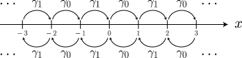
is, therefore, spatially 2-periodic, as shown in Fig. 1
Figure 1: The Hamiltonian given by Eqs. (2 3
We assume that the values of parameters γ 0 subscript 𝛾 0 \gamma_{0} γ 1 subscript 𝛾 1 \gamma_{1} γ 0 , γ 1 ≠ 0 subscript 𝛾 0 subscript 𝛾 1
0 \gamma_{0},\gamma_{1}\neq 0 | γ 0 | ≠ | γ 1 | subscript 𝛾 0 subscript 𝛾 1 |\gamma_{0}|\neq|\gamma_{1}| | γ 0 | = | γ 1 | subscript 𝛾 0 subscript 𝛾 1 |\gamma_{0}|=|\gamma_{1}| X t subscript 𝑋 𝑡 X_{t} t 𝑡 t x 𝑥 x t 𝑡 t
ℙ ( X t = x ) = | ψ t ( x ) | 2 . ℙ subscript 𝑋 𝑡 𝑥 superscript subscript 𝜓 𝑡 𝑥 2 \mathbb{P}(X_{t}=x)=\bigl{|}\psi_{t}(x)\bigr{|}^{2}. (6)
Let us introduce the Fourier transforms of the amplitude, represented by ψ ^ 0 , t ( k ) subscript ^ 𝜓 0 𝑡
𝑘 \hat{\psi}_{0,t}(k) ψ ^ 1 , t ( k ) ( k ∈ [ − π , π ) ) subscript ^ 𝜓 1 𝑡
𝑘 𝑘 𝜋 𝜋 \hat{\psi}_{1,t}(k)\,(k\in[-\pi,\pi))
ψ ^ 0 , t ( k ) = subscript ^ 𝜓 0 𝑡
𝑘 absent \displaystyle\hat{\psi}_{0,t}(k)= ∑ n ∈ ℤ e − i k ⋅ 2 n ψ t ( 2 n ) , subscript 𝑛 ℤ superscript 𝑒 ⋅ 𝑖 𝑘 2 𝑛 subscript 𝜓 𝑡 2 𝑛 \displaystyle\sum_{n\in\mathbb{Z}}e^{-ik\cdot 2n}\psi_{t}(2n), (7)
ψ ^ 1 , t ( k ) = subscript ^ 𝜓 1 𝑡
𝑘 absent \displaystyle\hat{\psi}_{1,t}(k)= ∑ n ∈ ℤ e − i k ⋅ ( 2 n + 1 ) ψ t ( 2 n + 1 ) . subscript 𝑛 ℤ superscript 𝑒 ⋅ 𝑖 𝑘 2 𝑛 1 subscript 𝜓 𝑡 2 𝑛 1 \displaystyle\sum_{n\in\mathbb{Z}}e^{-ik\cdot(2n+1)}\psi_{t}(2n+1). (8)
By the inverse Fourier transform, the Fourier transforms get back to the amplitude,
ψ t ( 2 n ) = subscript 𝜓 𝑡 2 𝑛 absent \displaystyle\psi_{t}(2n)= ∫ − π π e i k ⋅ 2 n ψ ^ 0 , t ( k ) d k 2 π , superscript subscript 𝜋 𝜋 superscript 𝑒 ⋅ 𝑖 𝑘 2 𝑛 subscript ^ 𝜓 0 𝑡
𝑘 𝑑 𝑘 2 𝜋 \displaystyle\int_{-\pi}^{\pi}e^{ik\cdot 2n}\hat{\psi}_{0,t}(k)\,\frac{dk}{2\pi}, (9)
ψ t ( 2 n + 1 ) = subscript 𝜓 𝑡 2 𝑛 1 absent \displaystyle\psi_{t}(2n+1)= ∫ − π π e i k ⋅ ( 2 n + 1 ) ψ ^ 1 , t ( k ) d k 2 π . superscript subscript 𝜋 𝜋 superscript 𝑒 ⋅ 𝑖 𝑘 2 𝑛 1 subscript ^ 𝜓 1 𝑡
𝑘 𝑑 𝑘 2 𝜋 \displaystyle\int_{-\pi}^{\pi}e^{ik\cdot(2n+1)}\hat{\psi}_{1,t}(k)\,\frac{dk}{2\pi}. (10)
Equations (2 3
i d d t ψ ^ 0 , t ( k ) = 𝑖 𝑑 𝑑 𝑡 subscript ^ 𝜓 0 𝑡
𝑘 absent \displaystyle i\,\frac{d}{dt}\hat{\psi}_{0,t}(k)= ( γ 1 e − i k + γ 0 e i k ) ψ ^ 1 , t ( k ) , subscript 𝛾 1 superscript 𝑒 𝑖 𝑘 subscript 𝛾 0 superscript 𝑒 𝑖 𝑘 subscript ^ 𝜓 1 𝑡
𝑘 \displaystyle(\gamma_{1}e^{-ik}+\gamma_{0}e^{ik})\hat{\psi}_{1,t}(k), (11)
i d d t ψ ^ 1 , t ( k ) = 𝑖 𝑑 𝑑 𝑡 subscript ^ 𝜓 1 𝑡
𝑘 absent \displaystyle i\,\frac{d}{dt}\hat{\psi}_{1,t}(k)= ( γ 0 e − i k + γ 1 e i k ) ψ ^ 0 , t ( k ) , subscript 𝛾 0 superscript 𝑒 𝑖 𝑘 subscript 𝛾 1 superscript 𝑒 𝑖 𝑘 subscript ^ 𝜓 0 𝑡
𝑘 \displaystyle(\gamma_{0}e^{-ik}+\gamma_{1}e^{ik})\hat{\psi}_{0,t}(k), (12)
and Eq. (1 ψ ^ 0 , 0 ( k ) = 1 subscript ^ 𝜓 0 0
𝑘 1 \hat{\psi}_{0,0}(k)=1 ψ ^ 1 , 0 ( k ) = 0 subscript ^ 𝜓 1 0
𝑘 0 \hat{\psi}_{1,0}(k)=0
4 Limit distribution
As many limit distributions have been derived for a scaled position by time t 𝑡 t
Theorem 1
Let ξ ∈ { 0 , 1 } 𝜉 0 1 \xi\in\left\{0,1\right\} | γ ξ | = min { | γ 0 | , | γ 1 | } subscript 𝛾 𝜉 subscript 𝛾 0 subscript 𝛾 1 |\gamma_{\xi}|=\min\left\{\,|\gamma_{0}|,|\gamma_{1}|\,\right\} x = 0 𝑥 0 x=0 t = 0 𝑡 0 t=0 ψ 0 ( 0 ) = 1 subscript 𝜓 0 0 1 \psi_{0}(0)=1 ψ 0 ( x ) = 0 ( x ≠ 0 ) subscript 𝜓 0 𝑥 0 𝑥 0 \psi_{0}(x)=0\,(x\neq 0) x 𝑥 x
lim t → ∞ ℙ ( X t t ≤ x ) = ∫ − ∞ x 1 π 4 γ ξ 2 − y 2 I ( − 2 | γ ξ | , 2 | γ ξ | ) ( y ) 𝑑 y , subscript → 𝑡 ℙ subscript 𝑋 𝑡 𝑡 𝑥 superscript subscript 𝑥 1 𝜋 4 superscript subscript 𝛾 𝜉 2 superscript 𝑦 2 subscript 𝐼 2 subscript 𝛾 𝜉 2 subscript 𝛾 𝜉 𝑦 differential-d 𝑦 \lim_{t\to\infty}\mathbb{P}\left(\frac{X_{t}}{t}\leq x\right)=\int_{-\infty}^{x}\frac{1}{\pi\sqrt{4\gamma_{\xi}^{2}-y^{2}}}I_{(\,-2|\gamma_{\xi}|,2|\gamma_{\xi}|\,)}(y)\,dy, (19)
where
I ( − 2 | γ ξ | , 2 | γ ξ | ) ( x ) = { 1 ( − 2 | γ ξ | < x < 2 | γ ξ | ) 0 ( otherwise ) . subscript 𝐼 2 subscript 𝛾 𝜉 2 subscript 𝛾 𝜉 𝑥 cases 1 2 subscript 𝛾 𝜉 bra 𝑥 bra 2 subscript 𝛾 𝜉 0 otherwise I_{(\,-2\,|\gamma_{\xi}|,2\,|\gamma_{\xi}|\,)}(x)=\left\{\begin{array}[]{cl}1&(\,-2\,|\gamma_{\xi}|<x<2\,|\gamma_{\xi}|\,)\\
0&(\mbox{otherwise})\end{array}\right.. (20)
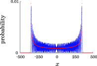
The limit theorem gives us an approximation of the probability as time t 𝑡 t
ℙ ( X t = x ) ∼ 1 π 4 γ ξ 2 t 2 − x 2 I ( − 2 | γ ξ | t , 2 | γ ξ | t ) ( x ) ( t → ∞ ) . similar-to ℙ subscript 𝑋 𝑡 𝑥 1 𝜋 4 superscript subscript 𝛾 𝜉 2 superscript 𝑡 2 superscript 𝑥 2 subscript 𝐼 2 subscript 𝛾 𝜉 𝑡 2 subscript 𝛾 𝜉 𝑡 𝑥 → 𝑡
\mathbb{P}(X_{t}=x)\sim\frac{1}{\pi\sqrt{4\gamma_{\xi}^{2}t^{2}-x^{2}}}I_{(-2|\gamma_{\xi}|t,2|\gamma_{\xi}|t)}(x)\quad(t\to\infty). (21)
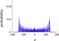
Figure 2 21 ℙ ( X t = x ) ℙ subscript 𝑋 𝑡 𝑥 \mathbb{P}(X_{t}=x) x = 0 𝑥 0 x=0
Figure 2: (Color figure online) The blue lines represent the probability distribution ℙ ( X t = x ) ℙ subscript 𝑋 𝑡 𝑥 \mathbb{P}(X_{t}=x) t = 500 𝑡 500 t=500 21 t = 500 𝑡 500 t=500 t 𝑡 t
The proof of Theorem 20 GrimmettJansonScudo2004
| ψ ^ t ( k ) ⟩ = ket subscript ^ 𝜓 𝑡 𝑘 absent \displaystyle\ket{\hat{\psi}_{t}(k)}= [ ψ ^ 0 , t ( k ) ψ ^ 1 , t ( k ) ] matrix subscript ^ 𝜓 0 𝑡
𝑘 subscript ^ 𝜓 1 𝑡
𝑘 \displaystyle\begin{bmatrix}\hat{\psi}_{0,t}(k)\\
\hat{\psi}_{1,t}(k)\end{bmatrix}
= \displaystyle= 1 2 I ( k ) e i g ( k ) ⋅ t [ I ( k ) − | I ( k ) | ] + 1 2 I ( k ) e − i g ( k ) ⋅ t [ I ( k ) | I ( k ) | ] , 1 2 𝐼 𝑘 superscript 𝑒 ⋅ 𝑖 𝑔 𝑘 𝑡 matrix 𝐼 𝑘 𝐼 𝑘 1 2 𝐼 𝑘 superscript 𝑒 ⋅ 𝑖 𝑔 𝑘 𝑡 matrix 𝐼 𝑘 𝐼 𝑘 \displaystyle\,\frac{1}{2I(k)}\,e^{i\sqrt{g(k)}\cdot t}\begin{bmatrix}I(k)\\
-|I(k)|\end{bmatrix}+\frac{1}{2I(k)}\,e^{-i\sqrt{g(k)}\cdot t}\begin{bmatrix}I(k)\\
|I(k)|\end{bmatrix}, (22)
we organize the r 𝑟 r 𝔼 [ X t r ] ( r = 0 , 1 , 2 , … ) 𝔼 delimited-[] superscript subscript 𝑋 𝑡 𝑟 𝑟 0 1 2 …
\mathbb{E}[X_{t}^{r}]\,(r=0,1,2,\ldots) t 𝑡 t D = i ⋅ d / d k 𝐷 ⋅ 𝑖 𝑑 𝑑 𝑘 D=i\cdot d/dk
D r | ψ ^ t ( k ) ⟩ = superscript 𝐷 𝑟 ket subscript ^ 𝜓 𝑡 𝑘 absent \displaystyle D^{r}\ket{\hat{\psi}_{t}(k)}= t r ⋅ e i g ( k ) ⋅ t ( − d d k g ( k ) ) r 1 2 I ( k ) [ I ( k ) − | I ( k ) | ] ⋅ superscript 𝑡 𝑟 superscript 𝑒 ⋅ 𝑖 𝑔 𝑘 𝑡 superscript 𝑑 𝑑 𝑘 𝑔 𝑘 𝑟 1 2 𝐼 𝑘 matrix 𝐼 𝑘 𝐼 𝑘 \displaystyle\,t^{r}\cdot e^{i\sqrt{g(k)}\cdot t}\left(-\frac{d}{dk}\sqrt{g(k)}\right)^{r}\,\frac{1}{2I(k)}\begin{bmatrix}I(k)\\
-|I(k)|\end{bmatrix}
+ t r ⋅ e − i g ( k ) ⋅ t ( d d k g ( k ) ) r 1 2 I ( k ) [ I ( k ) | I ( k ) | ] + O ( t r − 1 ) , ⋅ superscript 𝑡 𝑟 superscript 𝑒 ⋅ 𝑖 𝑔 𝑘 𝑡 superscript 𝑑 𝑑 𝑘 𝑔 𝑘 𝑟 1 2 𝐼 𝑘 matrix 𝐼 𝑘 𝐼 𝑘 𝑂 superscript 𝑡 𝑟 1 \displaystyle+\,t^{r}\cdot e^{-i\sqrt{g(k)}\cdot t}\left(\frac{d}{dk}\sqrt{g(k)}\right)^{r}\,\frac{1}{2I(k)}\begin{bmatrix}I(k)\\
|I(k)|\end{bmatrix}+O(t^{r-1}), (23)
the r 𝑟 r
𝔼 [ X t r ] = 𝔼 delimited-[] superscript subscript 𝑋 𝑡 𝑟 absent \displaystyle\mathbb{E}[X_{t}^{r}]= ∑ n ∈ ℤ ( 2 n ) r ℙ ( X t = 2 n ) + ∑ n ∈ ℤ ( 2 n + 1 ) r ℙ ( X t = 2 n + 1 ) subscript 𝑛 ℤ superscript 2 𝑛 𝑟 ℙ subscript 𝑋 𝑡 2 𝑛 subscript 𝑛 ℤ superscript 2 𝑛 1 𝑟 ℙ subscript 𝑋 𝑡 2 𝑛 1 \displaystyle\sum_{n\in\mathbb{Z}}\,(2n)^{r}\,\mathbb{P}(X_{t}=2n)+\sum_{n\in\mathbb{Z}}\,(2n+1)^{r}\,\mathbb{P}(X_{t}=2n+1)
= \displaystyle= ∫ − π π ψ ^ 0 , t ( k ) ¯ ( D r ψ ^ 0 , t ( k ) ) d k 2 π + ∫ − π π ψ ^ 1 , t ( k ) ¯ ( D r ψ ^ 1 , t ( k ) ) d k 2 π superscript subscript 𝜋 𝜋 ¯ subscript ^ 𝜓 0 𝑡
𝑘 superscript 𝐷 𝑟 subscript ^ 𝜓 0 𝑡
𝑘 𝑑 𝑘 2 𝜋 superscript subscript 𝜋 𝜋 ¯ subscript ^ 𝜓 1 𝑡
𝑘 superscript 𝐷 𝑟 subscript ^ 𝜓 1 𝑡
𝑘 𝑑 𝑘 2 𝜋 \displaystyle\int_{-\pi}^{\pi}\overline{\hat{\psi}_{0,t}(k)}\Bigl{(}D^{r}\hat{\psi}_{0,t}(k)\Bigr{)}\,\frac{dk}{2\pi}\,+\,\int_{-\pi}^{\pi}\overline{\hat{\psi}_{1,t}(k)}\Bigl{(}D^{r}\hat{\psi}_{1,t}(k)\Bigr{)}\,\frac{dk}{2\pi}
= \displaystyle= ∫ − π π ⟨ ψ ^ t ( k ) | ( D r | ψ ^ t ( k ) ⟩ ) d k 2 π superscript subscript 𝜋 𝜋 bra subscript ^ 𝜓 𝑡 𝑘 superscript 𝐷 𝑟 ket subscript ^ 𝜓 𝑡 𝑘 𝑑 𝑘 2 𝜋 \displaystyle\int_{-\pi}^{\pi}\bra{\hat{\psi}_{t}(k)}\Bigl{(}D^{r}\ket{\hat{\psi}_{t}(k)}\Bigr{)}\,\frac{dk}{2\pi}
= \displaystyle= t r { ∫ − π π ( d d k g ( k ) ) r d k 4 π + ∫ − π π ( − d d k g ( k ) ) r d k 4 π } + O ( t r − 1 ) . superscript 𝑡 𝑟 superscript subscript 𝜋 𝜋 superscript 𝑑 𝑑 𝑘 𝑔 𝑘 𝑟 𝑑 𝑘 4 𝜋 superscript subscript 𝜋 𝜋 superscript 𝑑 𝑑 𝑘 𝑔 𝑘 𝑟 𝑑 𝑘 4 𝜋 𝑂 superscript 𝑡 𝑟 1 \displaystyle\,t^{r}\,\left\{\int_{-\pi}^{\pi}\left(\frac{d}{dk}\sqrt{g(k)}\right)^{r}\,\frac{dk}{4\pi}+\int_{-\pi}^{\pi}\left(-\frac{d}{dk}\sqrt{g(k)}\right)^{r}\,\frac{dk}{4\pi}\right\}+O(t^{r-1}). (24)
One can derive the limits of the r 𝑟 r 𝔼 [ ( X t / t ) r ] 𝔼 delimited-[] superscript subscript 𝑋 𝑡 𝑡 𝑟 \mathbb{E}[(X_{t}/t)^{r}] t → ∞ → 𝑡 t\to\infty
lim t → ∞ 𝔼 [ ( X t t ) r ] = ∫ − π π ( − d d k g ( k ) ) r d k 4 π + ∫ − π π ( d d k g ( k ) ) r d k 4 π , subscript → 𝑡 𝔼 delimited-[] superscript subscript 𝑋 𝑡 𝑡 𝑟 superscript subscript 𝜋 𝜋 superscript 𝑑 𝑑 𝑘 𝑔 𝑘 𝑟 𝑑 𝑘 4 𝜋 superscript subscript 𝜋 𝜋 superscript 𝑑 𝑑 𝑘 𝑔 𝑘 𝑟 𝑑 𝑘 4 𝜋 \lim_{t\to\infty}\mathbb{E}\left[\left(\frac{X_{t}}{t}\right)^{r}\right]=\int_{-\pi}^{\pi}\left(-\frac{d}{dk}\sqrt{g(k)}\right)^{r}\,\frac{dk}{4\pi}+\int_{-\pi}^{\pi}\left(\frac{d}{dk}\sqrt{g(k)}\right)^{r}\,\frac{dk}{4\pi}, (25)
where
d d k g ( k ) = − 2 γ 0 γ 1 sin 2 k γ 0 2 + γ 1 2 + 2 γ 0 γ 1 cos 2 k . 𝑑 𝑑 𝑘 𝑔 𝑘 2 subscript 𝛾 0 subscript 𝛾 1 2 𝑘 superscript subscript 𝛾 0 2 superscript subscript 𝛾 1 2 2 subscript 𝛾 0 subscript 𝛾 1 2 𝑘 \frac{d}{dk}\sqrt{g(k)}=-\frac{2\gamma_{0}\gamma_{1}\sin 2k}{\sqrt{\gamma_{0}^{2}+\gamma_{1}^{2}+2\gamma_{0}\gamma_{1}\cos 2k}}. (26)
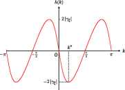
With h ( k ) = − d d k g ( k ) ℎ 𝑘 𝑑 𝑑 𝑘 𝑔 𝑘 h(k)=-\frac{d}{dk}\sqrt{g(k)}
∫ − π π ( ± h ( k ) ) r 𝑑 k = superscript subscript 𝜋 𝜋 superscript plus-or-minus ℎ 𝑘 𝑟 differential-d 𝑘 absent \displaystyle\int_{-\pi}^{\pi}\bigl{(}\pm h(k)\bigr{)}^{r}\,dk= ∫ − π 0 ( ± h ( k ) ) r 𝑑 k + ∫ 0 π ( ± h ( k ) ) r 𝑑 k superscript subscript 𝜋 0 superscript plus-or-minus ℎ 𝑘 𝑟 differential-d 𝑘 superscript subscript 0 𝜋 superscript plus-or-minus ℎ 𝑘 𝑟 differential-d 𝑘 \displaystyle\int_{-\pi}^{0}\bigl{(}\pm h(k)\bigr{)}^{r}\,dk+\int_{0}^{\pi}\bigl{(}\pm h(k)\bigr{)}^{r}\,dk
= \displaystyle= ∫ π 0 ( ± h ( − k ) ) r d ( − k ) + ∫ 0 π ( ± h ( k ) ) r 𝑑 k superscript subscript 𝜋 0 superscript plus-or-minus ℎ 𝑘 𝑟 𝑑 𝑘 superscript subscript 0 𝜋 superscript plus-or-minus ℎ 𝑘 𝑟 differential-d 𝑘 \displaystyle\int_{\pi}^{0}\bigl{(}\pm h(-k)\bigr{)}^{r}\,d(-k)+\int_{0}^{\pi}\bigl{(}\pm h(k)\bigr{)}^{r}\,dk
= \displaystyle= ∫ 0 π ( ∓ h ( k ) ) r 𝑑 k + ∫ 0 π ( ± h ( k ) ) r 𝑑 k , superscript subscript 0 𝜋 superscript minus-or-plus ℎ 𝑘 𝑟 differential-d 𝑘 superscript subscript 0 𝜋 superscript plus-or-minus ℎ 𝑘 𝑟 differential-d 𝑘 \displaystyle\int_{0}^{\pi}\bigl{(}\mp h(k)\bigr{)}^{r}\,dk+\int_{0}^{\pi}\bigl{(}\pm h(k)\bigr{)}^{r}\,dk, (27)
∫ 0 π ( ± h ( k ) ) r 𝑑 k = superscript subscript 0 𝜋 superscript plus-or-minus ℎ 𝑘 𝑟 differential-d 𝑘 absent \displaystyle\int_{0}^{\pi}\bigl{(}\pm h(k)\bigr{)}^{r}\,dk= ∫ 0 π 2 ( ± h ( k ) ) r 𝑑 k + ∫ π 2 π ( ± h ( k ) ) r 𝑑 k superscript subscript 0 𝜋 2 superscript plus-or-minus ℎ 𝑘 𝑟 differential-d 𝑘 superscript subscript 𝜋 2 𝜋 superscript plus-or-minus ℎ 𝑘 𝑟 differential-d 𝑘 \displaystyle\int_{0}^{\frac{\pi}{2}}\bigl{(}\pm h(k)\bigr{)}^{r}\,dk+\int_{\frac{\pi}{2}}^{\pi}\bigl{(}\pm h(k)\bigr{)}^{r}\,dk
= \displaystyle= ∫ 0 π 2 ( ± h ( k ) ) r 𝑑 k + ∫ π 2 0 ( ± h ( π − k ) ) r d ( π − k ) superscript subscript 0 𝜋 2 superscript plus-or-minus ℎ 𝑘 𝑟 differential-d 𝑘 superscript subscript 𝜋 2 0 superscript plus-or-minus ℎ 𝜋 𝑘 𝑟 𝑑 𝜋 𝑘 \displaystyle\int_{0}^{\frac{\pi}{2}}\bigl{(}\pm h(k)\bigr{)}^{r}\,dk+\int_{\frac{\pi}{2}}^{0}\bigl{(}\pm h(\pi-k)\bigr{)}^{r}\,d(\pi-k)
= \displaystyle= ∫ 0 π 2 ( ± h ( k ) ) r 𝑑 k + ∫ 0 π 2 ( ∓ h ( k ) ) r 𝑑 k , superscript subscript 0 𝜋 2 superscript plus-or-minus ℎ 𝑘 𝑟 differential-d 𝑘 superscript subscript 0 𝜋 2 superscript minus-or-plus ℎ 𝑘 𝑟 differential-d 𝑘 \displaystyle\int_{0}^{\frac{\pi}{2}}\bigl{(}\pm h(k)\bigr{)}^{r}\,dk+\int_{0}^{\frac{\pi}{2}}\bigl{(}\mp h(k)\bigr{)}^{r}\,dk, (28)
resulting in
∫ − π π ( ± h ( k ) ) r 𝑑 k = 2 { ∫ 0 π 2 ( ± h ( k ) ) r 𝑑 k + ∫ 0 π 2 ( ∓ h ( k ) ) r 𝑑 k } . superscript subscript 𝜋 𝜋 superscript plus-or-minus ℎ 𝑘 𝑟 differential-d 𝑘 2 superscript subscript 0 𝜋 2 superscript plus-or-minus ℎ 𝑘 𝑟 differential-d 𝑘 superscript subscript 0 𝜋 2 superscript minus-or-plus ℎ 𝑘 𝑟 differential-d 𝑘 \int_{-\pi}^{\pi}\bigl{(}\pm h(k)\bigr{)}^{r}\,dk=2\left\{\int_{0}^{\frac{\pi}{2}}\bigl{(}\pm h(k)\bigr{)}^{r}\,dk+\int_{0}^{\frac{\pi}{2}}\bigl{(}\mp h(k)\bigr{)}^{r}\,dk\right\}. (29)
Again, the r 𝑟 r
lim t → ∞ 𝔼 [ ( X t t ) r ] = 1 π { ∫ 0 π 2 h ( k ) r 𝑑 k + ∫ 0 π 2 ( − h ( k ) ) r 𝑑 k } , subscript → 𝑡 𝔼 delimited-[] superscript subscript 𝑋 𝑡 𝑡 𝑟 1 𝜋 superscript subscript 0 𝜋 2 ℎ superscript 𝑘 𝑟 differential-d 𝑘 superscript subscript 0 𝜋 2 superscript ℎ 𝑘 𝑟 differential-d 𝑘 \lim_{t\to\infty}\mathbb{E}\left[\left(\frac{X_{t}}{t}\right)^{r}\right]=\frac{1}{\pi}\left\{\int_{0}^{\frac{\pi}{2}}h(k)^{r}\,dk+\int_{0}^{\frac{\pi}{2}}\bigl{(}-h(k)\bigr{)}^{r}\,dk\right\}, (30)
where
h ( k ) = 2 γ 0 γ 1 sin 2 k γ 0 2 + γ 1 2 + 2 γ 0 γ 1 cos 2 k . ℎ 𝑘 2 subscript 𝛾 0 subscript 𝛾 1 2 𝑘 superscript subscript 𝛾 0 2 superscript subscript 𝛾 1 2 2 subscript 𝛾 0 subscript 𝛾 1 2 𝑘 h(k)=\frac{2\gamma_{0}\gamma_{1}\sin 2k}{\sqrt{\gamma_{0}^{2}+\gamma_{1}^{2}+2\gamma_{0}\gamma_{1}\cos 2k}}. (31)
Finding the derivative of h ( k ) ℎ 𝑘 h(k)
h ′ ( k ) = d d k h ( k ) = 4 γ 0 2 γ 1 2 g ( k ) g ( k ) ( cos 2 k + γ 1 γ 0 ) ( cos 2 k + γ 0 γ 1 ) , superscript ℎ ′ 𝑘 𝑑 𝑑 𝑘 ℎ 𝑘 4 superscript subscript 𝛾 0 2 superscript subscript 𝛾 1 2 𝑔 𝑘 𝑔 𝑘 2 𝑘 subscript 𝛾 1 subscript 𝛾 0 2 𝑘 subscript 𝛾 0 subscript 𝛾 1 h^{\prime}(k)=\frac{d}{dk}h(k)=\frac{4\gamma_{0}^{2}\gamma_{1}^{2}}{g(k)\sqrt{g(k)}}\left(\cos 2k+\frac{\gamma_{1}}{\gamma_{0}}\right)\left(\cos 2k+\frac{\gamma_{0}}{\gamma_{1}}\right), (32)
we realize that the function h ( k ) ℎ 𝑘 h(k) [ 0 , π / 2 ] 0 𝜋 2 [0,\pi/2] k = k ∗ ( ∈ [ 0 , π / 2 ] ) 𝑘 annotated superscript 𝑘 ∗ absent 0 𝜋 2 k=k^{\ast}\,(\in[0,\pi/2])
k ∗ = { 1 2 arccos ( − γ 1 γ 0 ) ( | γ 0 | > | γ 1 | ) 1 2 arccos ( − γ 0 γ 1 ) ( | γ 0 | < | γ 1 | ) , superscript 𝑘 ∗ cases 1 2 subscript 𝛾 1 subscript 𝛾 0 subscript 𝛾 0 subscript 𝛾 1 1 2 subscript 𝛾 0 subscript 𝛾 1 subscript 𝛾 0 subscript 𝛾 1 k^{\ast}=\left\{\begin{array}[]{ll}\displaystyle\frac{1}{2}\arccos\left(-\frac{\gamma_{1}}{\gamma_{0}}\right)&(\,|\gamma_{0}|>|\gamma_{1}|\,)\\[14.22636pt]
\displaystyle\frac{1}{2}\arccos\left(-\frac{\gamma_{0}}{\gamma_{1}}\right)&(\,|\gamma_{0}|<|\gamma_{1}|\,)\end{array}\right., (33)
h ( k ∗ ) = ℎ superscript 𝑘 ∗ absent \displaystyle h(k^{\ast})= { 2 | γ 1 | ⋅ γ 0 γ 1 | γ 0 γ 1 | ( | γ 0 | > | γ 1 | ) 2 | γ 0 | ⋅ γ 0 γ 1 | γ 0 γ 1 | ( | γ 0 | < | γ 1 | ) cases ⋅ 2 subscript 𝛾 1 subscript 𝛾 0 subscript 𝛾 1 subscript 𝛾 0 subscript 𝛾 1 subscript 𝛾 0 subscript 𝛾 1 ⋅ 2 subscript 𝛾 0 subscript 𝛾 0 subscript 𝛾 1 subscript 𝛾 0 subscript 𝛾 1 subscript 𝛾 0 subscript 𝛾 1 \displaystyle\left\{\begin{array}[]{ll}\displaystyle 2\,|\gamma_{1}|\cdot\frac{\gamma_{0}\gamma_{1}}{\,|\gamma_{0}\gamma_{1}|\,}&(\,|\gamma_{0}|>|\gamma_{1}|\,)\\[14.22636pt]
\displaystyle 2\,|\gamma_{0}|\cdot\frac{\gamma_{0}\gamma_{1}}{\,|\gamma_{0}\gamma_{1}|\,}&(\,|\gamma_{0}|<|\gamma_{1}|\,)\end{array}\right. (36)
= \displaystyle= 2 | γ ξ | ⋅ γ 0 γ 1 | γ 0 γ 1 | ⋅ 2 subscript 𝛾 𝜉 subscript 𝛾 0 subscript 𝛾 1 subscript 𝛾 0 subscript 𝛾 1 \displaystyle 2\,|\gamma_{\xi}|\cdot\frac{\gamma_{0}\gamma_{1}}{\,|\gamma_{0}\gamma_{1}|\,}
= \displaystyle= { 2 | γ ξ | ( γ 0 γ 1 > 0 ) − 2 | γ ξ | ( γ 0 γ 1 < 0 ) , cases 2 subscript 𝛾 𝜉 subscript 𝛾 0 subscript 𝛾 1 0 2 subscript 𝛾 𝜉 subscript 𝛾 0 subscript 𝛾 1 0 \displaystyle\left\{\begin{array}[]{rl}2\,|\gamma_{\xi}|&\quad(\gamma_{0}\gamma_{1}>0)\\
-2\,|\gamma_{\xi}|&\quad(\gamma_{0}\gamma_{1}<0)\end{array}\right., (39)
where ξ ∈ { 0 , 1 } 𝜉 0 1 \xi\in\left\{0,1\right\} | γ ξ | = min { | γ 0 | , | γ 1 | } subscript 𝛾 𝜉 subscript 𝛾 0 subscript 𝛾 1 |\gamma_{\xi}|=\min\left\{\,|\gamma_{0}|,|\gamma_{1}|\,\right\}
{ h ′ ( k ) > 0 ( k ∈ [ 0 , k ∗ ) ) h ′ ( k ) < 0 ( k ∈ ( k ∗ , π / 2 ] ) ( γ 0 γ 1 > 0 ) , cases superscript ℎ ′ 𝑘 0 𝑘 0 superscript 𝑘 ∗ missing-subexpression superscript ℎ ′ 𝑘 0 𝑘 superscript 𝑘 ∗ 𝜋 2 missing-subexpression subscript 𝛾 0 subscript 𝛾 1 0
\displaystyle\left\{\begin{array}[]{lll}h^{\prime}(k)>0&(k\in[0,k^{\ast}))\\
h^{\prime}(k)<0&(k\in(k^{\ast},\pi/2])\\
\end{array}\right.\quad(\gamma_{0}\gamma_{1}>0), (42)
{ h ′ ( k ) < 0 ( k ∈ [ 0 , k ∗ ) ) h ′ ( k ) > 0 ( k ∈ ( k ∗ , π / 2 ] ) ( γ 0 γ 1 < 0 ) . cases superscript ℎ ′ 𝑘 0 𝑘 0 superscript 𝑘 ∗ missing-subexpression superscript ℎ ′ 𝑘 0 𝑘 superscript 𝑘 ∗ 𝜋 2 missing-subexpression subscript 𝛾 0 subscript 𝛾 1 0
\displaystyle\left\{\begin{array}[]{lll}h^{\prime}(k)<0&(k\in[0,k^{\ast}))\\
h^{\prime}(k)>0&(k\in(k^{\ast},\pi/2])\\
\end{array}\right.\quad(\gamma_{0}\gamma_{1}<0). (45)
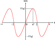
The function h ( k ) ℎ 𝑘 h(k) π 𝜋 \pi h ( π − k ) = − h ( k ) ℎ 𝜋 𝑘 ℎ 𝑘 h(\pi-k)=-h(k) h ( k ∗ ) ℎ superscript 𝑘 ∗ h(k^{\ast}) h ( k ) ℎ 𝑘 h(k) γ 0 γ 1 subscript 𝛾 0 subscript 𝛾 1 \gamma_{0}\gamma_{1} 3 h ( k ) ℎ 𝑘 h(k) [ − π , π ] 𝜋 𝜋 [-\pi,\pi]
Figure 3: (Color figure online) The function h ( k ) ℎ 𝑘 h(k) π 𝜋 \pi γ 0 subscript 𝛾 0 \gamma_{0} γ 1 subscript 𝛾 1 \gamma_{1} [ − 2 | γ ξ | , 2 | γ ξ | ] 2 subscript 𝛾 𝜉 2 subscript 𝛾 𝜉 \bigl{[}-2\,|\gamma_{\xi}|\,,2\,|\gamma_{\xi}|\,\bigr{]}
Substituting h ( k ) = x ℎ 𝑘 𝑥 h(k)=x
∫ 0 π 2 ( ± h ( k ) ) r 𝑑 k = superscript subscript 0 𝜋 2 superscript plus-or-minus ℎ 𝑘 𝑟 differential-d 𝑘 absent \displaystyle\int_{0}^{\frac{\pi}{2}}\Bigl{(}\pm h(k)\Bigr{)}^{r}\,dk= ∫ 0 k ∗ ( ± h ( k ) ) r 𝑑 k + ∫ k ∗ π 2 ( ± h ( k ) ) r 𝑑 k superscript subscript 0 superscript 𝑘 ∗ superscript plus-or-minus ℎ 𝑘 𝑟 differential-d 𝑘 superscript subscript superscript 𝑘 ∗ 𝜋 2 superscript plus-or-minus ℎ 𝑘 𝑟 differential-d 𝑘 \displaystyle\int_{0}^{k^{\ast}}\Bigl{(}\pm h(k)\Bigr{)}^{r}\,dk+\int_{k^{\ast}}^{\frac{\pi}{2}}\Bigl{(}\pm h(k)\Bigr{)}^{r}\,dk
= \displaystyle= ∫ 0 h ( k ∗ ) ( ± x ) r d k + ( x ) d x 𝑑 x + ∫ h ( k ∗ ) 0 ( ± x ) r d k − ( x ) d x 𝑑 x superscript subscript 0 ℎ superscript 𝑘 ∗ superscript plus-or-minus 𝑥 𝑟 𝑑 subscript 𝑘 𝑥 𝑑 𝑥 differential-d 𝑥 superscript subscript ℎ superscript 𝑘 ∗ 0 superscript plus-or-minus 𝑥 𝑟 𝑑 subscript 𝑘 𝑥 𝑑 𝑥 differential-d 𝑥 \displaystyle\int_{0}^{h(k^{\ast})}(\pm x)^{r}\frac{dk_{+}(x)}{dx}\,dx+\int_{h(k^{\ast})}^{0}(\pm x)^{r}\frac{dk_{-}(x)}{dx}\,dx
= \displaystyle= ∫ 0 h ( k ∗ ) ( ± x ) r ( d k + ( x ) d x − d k − ( x ) d x ) 𝑑 x , superscript subscript 0 ℎ superscript 𝑘 ∗ superscript plus-or-minus 𝑥 𝑟 𝑑 subscript 𝑘 𝑥 𝑑 𝑥 𝑑 subscript 𝑘 𝑥 𝑑 𝑥 differential-d 𝑥 \displaystyle\int_{0}^{h(k^{\ast})}(\pm x)^{r}\biggl{(}\frac{dk_{+}(x)}{dx}-\frac{dk_{-}(x)}{dx}\biggr{)}\,dx, (46)
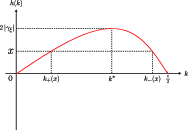
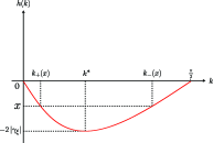
where the functions k ± ( x ) ( ∈ [ 0 , π / 2 ] ) annotated subscript 𝑘 plus-or-minus 𝑥 absent 0 𝜋 2 k_{\pm}(x)\,(\in[0,\pi/2]\,) h ( k ± ( x ) ) = x ℎ subscript 𝑘 plus-or-minus 𝑥 𝑥 h(k_{\pm}(x))=x 4
k ± ( x ) = { 1 2 arccos ( − x 2 ± 4 γ 0 2 − x 2 4 γ 1 2 − x 2 4 γ 0 γ 1 ) ( γ 0 γ 1 > 0 ) 1 2 arccos ( − x 2 ∓ 4 γ 0 2 − x 2 4 γ 1 2 − x 2 4 γ 0 γ 1 ) ( γ 0 γ 1 < 0 ) , subscript 𝑘 plus-or-minus 𝑥 cases 1 2 plus-or-minus superscript 𝑥 2 4 superscript subscript 𝛾 0 2 superscript 𝑥 2 4 superscript subscript 𝛾 1 2 superscript 𝑥 2 4 subscript 𝛾 0 subscript 𝛾 1 subscript 𝛾 0 subscript 𝛾 1 0 1 2 minus-or-plus superscript 𝑥 2 4 superscript subscript 𝛾 0 2 superscript 𝑥 2 4 superscript subscript 𝛾 1 2 superscript 𝑥 2 4 subscript 𝛾 0 subscript 𝛾 1 subscript 𝛾 0 subscript 𝛾 1 0 k_{\pm}(x)=\left\{\begin{array}[]{ll}\displaystyle\frac{1}{2}\arccos\left(\frac{-x^{2}\pm\sqrt{4\gamma_{0}^{2}-x^{2}}\sqrt{4\gamma_{1}^{2}-x^{2}}}{4\gamma_{0}\gamma_{1}}\right)&(\gamma_{0}\gamma_{1}>0)\\[14.22636pt]
\displaystyle\frac{1}{2}\arccos\left(\frac{-x^{2}\mp\sqrt{4\gamma_{0}^{2}-x^{2}}\sqrt{4\gamma_{1}^{2}-x^{2}}}{4\gamma_{0}\gamma_{1}}\right)&(\gamma_{0}\gamma_{1}<0)\end{array}\right., (47)
whose derivatives are computed and organized,
d d x ( 1 2 arccos ( − x 2 ± 4 γ 0 2 − x 2 4 γ 1 2 − x 2 4 γ 0 γ 1 ) ) 𝑑 𝑑 𝑥 1 2 plus-or-minus superscript 𝑥 2 4 superscript subscript 𝛾 0 2 superscript 𝑥 2 4 superscript subscript 𝛾 1 2 superscript 𝑥 2 4 subscript 𝛾 0 subscript 𝛾 1 \displaystyle\frac{d}{dx}\left(\frac{1}{2}\arccos\left(\frac{-x^{2}\pm\sqrt{4\gamma_{0}^{2}-x^{2}}\sqrt{4\gamma_{1}^{2}-x^{2}}}{4\gamma_{0}\gamma_{1}}\right)\right)
= \displaystyle= ± 1 2 ⋅ x | x | ⋅ | γ 0 γ 1 | γ 0 γ 1 ⋅ | 4 γ 0 2 − x 2 ± 4 γ 1 2 − x 2 | 4 γ 0 2 − x 2 4 γ 1 2 − x 2 plus-or-minus ⋅ 1 2 𝑥 𝑥 subscript 𝛾 0 subscript 𝛾 1 subscript 𝛾 0 subscript 𝛾 1 plus-or-minus 4 superscript subscript 𝛾 0 2 superscript 𝑥 2 4 superscript subscript 𝛾 1 2 superscript 𝑥 2 4 superscript subscript 𝛾 0 2 superscript 𝑥 2 4 superscript subscript 𝛾 1 2 superscript 𝑥 2 \displaystyle\pm\frac{1}{2}\cdot\frac{x}{\,|x|\,}\cdot\frac{\,|\gamma_{0}\gamma_{1}|\,}{\gamma_{0}\gamma_{1}}\cdot\frac{\,\Bigl{|}\,\sqrt{4\gamma_{0}^{2}-x^{2}}\pm\sqrt{4\gamma_{1}^{2}-x^{2}}\,\Bigr{|}\,}{\sqrt{4\gamma_{0}^{2}-x^{2}}\sqrt{4\gamma_{1}^{2}-x^{2}}}
= : absent : \displaystyle=: f ± ( x ) . subscript 𝑓 plus-or-minus 𝑥 \displaystyle\,f_{\pm}(x). (48)
Figure 4: (Color figure online) The functions k ± ( x ) ( ∈ [ 0 , π / 2 ] ) annotated subscript 𝑘 plus-or-minus 𝑥 absent 0 𝜋 2 k_{\pm}(x)\,(\in[0,\pi/2]\,) h ( k ± ( x ) ) = x ℎ subscript 𝑘 plus-or-minus 𝑥 𝑥 h(k_{\pm}(x))=x
Note that the equation h ( k ) = x ( k ∈ [ 0 , π / 2 ] ) ℎ 𝑘 𝑥 𝑘 0 𝜋 2 h(k)=x\,(k\in[0,\pi/2]\,) x ∈ [ 0 , 2 | γ ξ | ] ( γ 0 γ 1 > 0 ) 𝑥 0 2 subscript 𝛾 𝜉 subscript 𝛾 0 subscript 𝛾 1 0 x\in[\,0,2\,|\gamma_{\xi}|\,]\,(\gamma_{0}\gamma_{1}>0) x ∈ [ − 2 | γ ξ | , 0 ] ( γ 0 γ 1 < 0 ) 𝑥 2 subscript 𝛾 𝜉 0 subscript 𝛾 0 subscript 𝛾 1 0 x\in[\,-2\,|\gamma_{\xi}|,0\,]\,(\gamma_{0}\gamma_{1}<0) k ± ( x ) subscript 𝑘 plus-or-minus 𝑥 k_{\pm}(x) k + ( x ) ≤ k − ( x ) subscript 𝑘 𝑥 subscript 𝑘 𝑥 k_{+}(x)\leq k_{-}(x)
Let us wrap up the computation,
∫ 0 π 2 h ( k ) r 𝑑 k + ∫ 0 π 2 ( − h ( k ) ) r 𝑑 k superscript subscript 0 𝜋 2 ℎ superscript 𝑘 𝑟 differential-d 𝑘 superscript subscript 0 𝜋 2 superscript ℎ 𝑘 𝑟 differential-d 𝑘 \displaystyle\int_{0}^{\frac{\pi}{2}}h(k)^{r}\,dk+\int_{0}^{\frac{\pi}{2}}\bigl{(}-h(k)\bigr{)}^{r}\,dk
= \displaystyle= { ∫ 0 h ( k ∗ ) x r ( f + ( x ) − f − ( x ) ) 𝑑 x + ∫ h ( k ∗ ) 0 ( − x ) r { − ( f + ( x ) − f − ( x ) ) } 𝑑 x ( γ 0 γ 1 > 0 ) ∫ 0 h ( k ∗ ) x r ( f − ( x ) − f + ( x ) ) 𝑑 x + ∫ h ( k ∗ ) 0 ( − x ) r { − ( f − ( x ) − f + ( x ) ) } 𝑑 x ( γ 0 γ 1 < 0 ) cases superscript subscript 0 ℎ superscript 𝑘 ∗ superscript 𝑥 𝑟 subscript 𝑓 𝑥 subscript 𝑓 𝑥 differential-d 𝑥 superscript subscript ℎ superscript 𝑘 ∗ 0 superscript 𝑥 𝑟 subscript 𝑓 𝑥 subscript 𝑓 𝑥 differential-d 𝑥 subscript 𝛾 0 subscript 𝛾 1 0 superscript subscript 0 ℎ superscript 𝑘 ∗ superscript 𝑥 𝑟 subscript 𝑓 𝑥 subscript 𝑓 𝑥 differential-d 𝑥 superscript subscript ℎ superscript 𝑘 ∗ 0 superscript 𝑥 𝑟 subscript 𝑓 𝑥 subscript 𝑓 𝑥 differential-d 𝑥 subscript 𝛾 0 subscript 𝛾 1 0 \displaystyle\left\{\begin{array}[]{r}\displaystyle\int_{0}^{h(k^{\ast})}x^{r}\,\bigl{(}f_{+}(x)-f_{-}(x)\bigr{)}\,dx+\int_{h(k^{\ast})}^{0}(-x)^{r}\,\Bigl{\{}-\bigl{(}f_{+}(x)-f_{-}(x)\bigr{)}\Bigr{\}}\,dx\\
(\gamma_{0}\gamma_{1}>0)\\[8.53581pt]
\displaystyle\int_{0}^{h(k^{\ast})}x^{r}\,\bigl{(}f_{-}(x)-f_{+}(x)\bigr{)}\,dx+\int_{h(k^{\ast})}^{0}(-x)^{r}\,\Bigl{\{}-\bigl{(}f_{-}(x)-f_{+}(x)\bigr{)}\Bigr{\}}\,dx\\
(\gamma_{0}\gamma_{1}<0)\end{array}\right. (53)
= \displaystyle= { ∫ 0 h ( k ∗ ) x r ( f + ( x ) − f − ( x ) ) 𝑑 x + ∫ − h ( k ∗ ) 0 x r { − ( f + ( − x ) − f − ( − x ) ) } d ( − x ) ( γ 0 γ 1 > 0 ) ∫ 0 h ( k ∗ ) x r ( f − ( x ) − f + ( x ) ) 𝑑 x + ∫ − h ( k ∗ ) 0 x r { − ( f − ( − x ) − f + ( − x ) ) } d ( − x ) ( γ 0 γ 1 < 0 ) cases superscript subscript 0 ℎ superscript 𝑘 ∗ superscript 𝑥 𝑟 subscript 𝑓 𝑥 subscript 𝑓 𝑥 differential-d 𝑥 superscript subscript ℎ superscript 𝑘 ∗ 0 superscript 𝑥 𝑟 subscript 𝑓 𝑥 subscript 𝑓 𝑥 𝑑 𝑥 subscript 𝛾 0 subscript 𝛾 1 0 superscript subscript 0 ℎ superscript 𝑘 ∗ superscript 𝑥 𝑟 subscript 𝑓 𝑥 subscript 𝑓 𝑥 differential-d 𝑥 superscript subscript ℎ superscript 𝑘 ∗ 0 superscript 𝑥 𝑟 subscript 𝑓 𝑥 subscript 𝑓 𝑥 𝑑 𝑥 subscript 𝛾 0 subscript 𝛾 1 0 \displaystyle\left\{\begin{array}[]{r}\displaystyle\int_{0}^{h(k^{\ast})}x^{r}\,\bigl{(}f_{+}(x)-f_{-}(x)\bigr{)}\,dx+\int_{-h(k^{\ast})}^{0}x^{r}\,\Bigl{\{}-\bigl{(}f_{+}(-x)-f_{-}(-x)\bigr{)}\Bigr{\}}\,d(-x)\\
(\gamma_{0}\gamma_{1}>0)\\[8.53581pt]
\displaystyle\int_{0}^{h(k^{\ast})}x^{r}\,\bigl{(}f_{-}(x)-f_{+}(x)\bigr{)}\,dx+\int_{-h(k^{\ast})}^{0}x^{r}\,\Bigl{\{}-\bigl{(}f_{-}(-x)-f_{+}(-x)\bigr{)}\Bigr{\}}\,d(-x)\\
(\gamma_{0}\gamma_{1}<0)\end{array}\right. (58)
= \displaystyle= { ∫ 0 2 | γ ξ | x r 1 4 γ ξ 2 − x 2 𝑑 x + ∫ − 2 | γ ξ | 0 x r 1 4 γ ξ 2 − x 2 𝑑 x ( γ 0 γ 1 > 0 ) ∫ 0 − 2 | γ ξ | x r ( − 1 4 γ ξ 2 − x 2 ) 𝑑 x + ∫ 2 | γ ξ | 0 x r ( − 1 4 γ ξ 2 − x 2 ) 𝑑 x ( γ 0 γ 1 < 0 ) cases superscript subscript 0 2 subscript 𝛾 𝜉 superscript 𝑥 𝑟 1 4 superscript subscript 𝛾 𝜉 2 superscript 𝑥 2 differential-d 𝑥 superscript subscript 2 subscript 𝛾 𝜉 0 superscript 𝑥 𝑟 1 4 superscript subscript 𝛾 𝜉 2 superscript 𝑥 2 differential-d 𝑥 subscript 𝛾 0 subscript 𝛾 1 0 superscript subscript 0 2 subscript 𝛾 𝜉 superscript 𝑥 𝑟 1 4 superscript subscript 𝛾 𝜉 2 superscript 𝑥 2 differential-d 𝑥 superscript subscript 2 subscript 𝛾 𝜉 0 superscript 𝑥 𝑟 1 4 superscript subscript 𝛾 𝜉 2 superscript 𝑥 2 differential-d 𝑥 subscript 𝛾 0 subscript 𝛾 1 0 \displaystyle\left\{\begin{array}[]{l}\displaystyle\int_{0}^{2\,|\gamma_{\xi}|}x^{r}\,\frac{1}{\sqrt{4\gamma_{\xi}^{2}-x^{2}}}\,dx+\int_{-2\,|\gamma_{\xi}|}^{0}x^{r}\,\frac{1}{\sqrt{4\gamma_{\xi}^{2}-x^{2}}}\,dx\\
(\gamma_{0}\gamma_{1}>0)\\[8.53581pt]
\displaystyle\int_{0}^{-2\,|\gamma_{\xi}|}x^{r}\,\left(-\,\frac{1}{\sqrt{4\gamma_{\xi}^{2}-x^{2}}}\right)\,dx+\int_{2\,|\gamma_{\xi}|}^{0}x^{r}\,\left(-\,\frac{1}{\sqrt{4\gamma_{\xi}^{2}-x^{2}}}\right)\,dx\\
(\gamma_{0}\gamma_{1}<0)\end{array}\right. (63)
= \displaystyle= ∫ − 2 | γ ξ | 2 | γ ξ | x r 1 4 γ ξ 2 − x 2 𝑑 x , superscript subscript 2 subscript 𝛾 𝜉 2 subscript 𝛾 𝜉 superscript 𝑥 𝑟 1 4 superscript subscript 𝛾 𝜉 2 superscript 𝑥 2 differential-d 𝑥 \displaystyle\int_{-2\,|\gamma_{\xi}|}^{2\,|\gamma_{\xi}|}x^{r}\,\frac{1}{\sqrt{4\gamma_{\xi}^{2}-x^{2}}}\,dx, (64)
in which we have used
f + ( x ) − f − ( x ) subscript 𝑓 𝑥 subscript 𝑓 𝑥 \displaystyle f_{+}(x)-f_{-}(x)
= \displaystyle= 1 2 ⋅ x | x | ⋅ | γ 0 γ 1 | γ 0 γ 1 ⋅ | 4 γ 0 2 − x 2 + 4 γ 1 2 − x 2 | + | 4 γ 0 2 − x 2 − 4 γ 1 2 − x 2 | 4 γ 0 2 − x 2 4 γ 1 2 − x 2 \displaystyle\,\frac{1}{2}\cdot\frac{x}{\,|x|\,}\cdot\frac{\,|\gamma_{0}\gamma_{1}|\,}{\gamma_{0}\gamma_{1}}\cdot\frac{\,\Bigl{|}\,\sqrt{4\gamma_{0}^{2}-x^{2}}+\sqrt{4\gamma_{1}^{2}-x^{2}}\,\Bigr{|}\,+\,\Bigl{|}\sqrt{4\gamma_{0}^{2}-x^{2}}-\sqrt{4\gamma_{1}^{2}-x^{2}}\,\Bigr{|}\,}{\sqrt{4\gamma_{0}^{2}-x^{2}}\sqrt{4\gamma_{1}^{2}-x^{2}}}
= \displaystyle= { x | x | ⋅ | γ 0 γ 1 | γ 0 γ 1 ⋅ 1 4 γ 1 2 − x 2 ( | γ 0 | > | γ 1 | ) x | x | ⋅ | γ 0 γ 1 | γ 0 γ 1 ⋅ 1 4 γ 0 2 − x 2 ( | γ 0 | < | γ 1 | ) cases ⋅ 𝑥 𝑥 subscript 𝛾 0 subscript 𝛾 1 subscript 𝛾 0 subscript 𝛾 1 1 4 superscript subscript 𝛾 1 2 superscript 𝑥 2 subscript 𝛾 0 subscript 𝛾 1 ⋅ 𝑥 𝑥 subscript 𝛾 0 subscript 𝛾 1 subscript 𝛾 0 subscript 𝛾 1 1 4 superscript subscript 𝛾 0 2 superscript 𝑥 2 subscript 𝛾 0 subscript 𝛾 1 \displaystyle\left\{\begin{array}[]{ll}\displaystyle\frac{x}{\,|x|\,}\cdot\frac{\,|\gamma_{0}\gamma_{1}|\,}{\gamma_{0}\gamma_{1}}\cdot\frac{1}{\sqrt{4\gamma_{1}^{2}-x^{2}}}&\quad(\,|\gamma_{0}|>|\gamma_{1}|\,)\\[14.22636pt]
\displaystyle\frac{x}{\,|x|\,}\cdot\frac{\,|\gamma_{0}\gamma_{1}|\,}{\gamma_{0}\gamma_{1}}\cdot\frac{1}{\sqrt{4\gamma_{0}^{2}-x^{2}}}&\quad(\,|\gamma_{0}|<|\gamma_{1}|\,)\end{array}\right. (67)
= \displaystyle= x | x | ⋅ | γ 0 γ 1 | γ 0 γ 1 ⋅ 1 4 γ ξ 2 − x 2 . ⋅ 𝑥 𝑥 subscript 𝛾 0 subscript 𝛾 1 subscript 𝛾 0 subscript 𝛾 1 1 4 superscript subscript 𝛾 𝜉 2 superscript 𝑥 2 \displaystyle\frac{x}{\,|x|\,}\cdot\frac{\,|\gamma_{0}\gamma_{1}|\,}{\gamma_{0}\gamma_{1}}\cdot\frac{1}{\sqrt{4\gamma_{\xi}^{2}-x^{2}}}. (68)
Reminding Eq. (30 r 𝑟 r
lim t → ∞ 𝔼 [ ( X t t ) r ] = subscript → 𝑡 𝔼 delimited-[] superscript subscript 𝑋 𝑡 𝑡 𝑟 absent \displaystyle\lim_{t\to\infty}\mathbb{E}\left[\left(\frac{X_{t}}{t}\right)^{r}\right]= ∫ − 2 | γ ξ | 2 | γ ξ | x r 1 π 4 γ ξ 2 − x 2 𝑑 x superscript subscript 2 subscript 𝛾 𝜉 2 subscript 𝛾 𝜉 superscript 𝑥 𝑟 1 𝜋 4 superscript subscript 𝛾 𝜉 2 superscript 𝑥 2 differential-d 𝑥 \displaystyle\int_{-2\,|\gamma_{\xi}|}^{2\,|\gamma_{\xi}|}x^{r}\,\frac{1}{\pi\sqrt{4\gamma_{\xi}^{2}-x^{2}}}\,dx
= \displaystyle= ∫ − ∞ ∞ x r 1 π 4 γ ξ 2 − x 2 I ( − 2 | γ ξ | , 2 | γ ξ | ) 𝑑 x , superscript subscript superscript 𝑥 𝑟 1 𝜋 4 superscript subscript 𝛾 𝜉 2 superscript 𝑥 2 subscript 𝐼 2 subscript 𝛾 𝜉 2 subscript 𝛾 𝜉 differential-d 𝑥 \displaystyle\int_{-\infty}^{\infty}x^{r}\,\frac{1}{\pi\sqrt{4\gamma_{\xi}^{2}-x^{2}}}\,I_{(\,-2\,|\gamma_{\xi}|,2\,|\gamma_{\xi}|\,)}\,dx, (69)
where
I ( − 2 | γ ξ | , 2 | γ ξ | ) ( x ) = { 1 ( − 2 | γ ξ | < x < 2 | γ ξ | ) 0 ( otherwise ) . subscript 𝐼 2 subscript 𝛾 𝜉 2 subscript 𝛾 𝜉 𝑥 cases 1 2 subscript 𝛾 𝜉 bra 𝑥 bra 2 subscript 𝛾 𝜉 0 otherwise I_{(\,-2\,|\gamma_{\xi}|,2\,|\gamma_{\xi}|\,)}(x)=\left\{\begin{array}[]{cl}1&(\,-2\,|\gamma_{\xi}|<x<2\,|\gamma_{\xi}|\,)\\
0&(\mbox{otherwise})\end{array}\right.. (70)
Equation (69 20
5 Summary
We studied a continuous-time quantum walk on ℤ = { 0 , ± 1 , ± 2 , … } ℤ 0 plus-or-minus 1 plus-or-minus 2 … \mathbb{Z}=\left\{0,\pm 1,\pm 2,\ldots\right\} { ψ t ( x ) : x ∈ ℤ } conditional-set subscript 𝜓 𝑡 𝑥 𝑥 ℤ \left\{\psi_{t}(x):x\in\mathbb{Z}\right\} X t / t subscript 𝑋 𝑡 𝑡 X_{t}/t t → ∞ → 𝑡 t\to\infty ℙ ( X t = x ) ℙ subscript 𝑋 𝑡 𝑥 \mathbb{P}(X_{t}=x) t 𝑡 t γ 0 subscript 𝛾 0 \gamma_{0} γ 1 subscript 𝛾 1 \gamma_{1} γ 0 subscript 𝛾 0 \gamma_{0} γ 1 subscript 𝛾 1 \gamma_{1} γ ξ subscript 𝛾 𝜉 \gamma_{\xi} | γ ξ | = min { | γ 0 | , | γ 1 | } subscript 𝛾 𝜉 subscript 𝛾 0 subscript 𝛾 1 |\gamma_{\xi}|=\min\left\{\,|\gamma_{0}|,\,|\gamma_{1}|\,\right\}
A similar property was also reported for discrete-time quantum walks in the past studies MachidaKonno2010 ; MachidaGrunbaum2018 MachidaKonno2010 ℤ ℤ \mathbb{Z} MachidaGrunbaum2018 ℤ ℤ \mathbb{Z}
Although two parameters operated the continuous-time quantum walk, one parameter did not affect the quantum walker in approximation as time t 𝑡 t
The author is supported by JSPS Grant-in-Aid for Scientific Research (C) (No. 23K03220).
Appendix A | γ 0 | = | γ 1 | subscript 𝛾 0 subscript 𝛾 1 |\gamma_{0}|=|\gamma_{1}|
We briefly see the continuous-time quantum walk in the case of | γ 0 | = | γ 1 | subscript 𝛾 0 subscript 𝛾 1 |\gamma_{0}|=|\gamma_{1}| γ 1 = ± γ 0 subscript 𝛾 1 plus-or-minus subscript 𝛾 0 \gamma_{1}=\pm\gamma_{0} 3 4 | γ 0 | = | γ 1 | subscript 𝛾 0 subscript 𝛾 1 |\gamma_{0}|=|\gamma_{1}|
h ( k ) = 2 γ 0 γ 1 sin 2 k γ 0 2 + γ 1 2 + 2 γ 0 γ 1 cos 2 k ( k ∈ [ − π , π ) ) , ℎ 𝑘 2 subscript 𝛾 0 subscript 𝛾 1 2 𝑘 superscript subscript 𝛾 0 2 superscript subscript 𝛾 1 2 2 subscript 𝛾 0 subscript 𝛾 1 2 𝑘 𝑘 𝜋 𝜋
h(k)=\frac{2\gamma_{0}\gamma_{1}\sin 2k}{\sqrt{\gamma_{0}^{2}+\gamma_{1}^{2}+2\gamma_{0}\gamma_{1}\cos 2k}}\quad(k\in[-\pi,\pi)), (71)
becomes zero at k = ± π / 2 𝑘 plus-or-minus 𝜋 2 k=\pm\pi/2 k = − π , 0 𝑘 𝜋 0
k=-\pi,0 γ 1 = γ 0 subscript 𝛾 1 subscript 𝛾 0 \gamma_{1}=\gamma_{0} γ 1 = − γ 0 subscript 𝛾 1 subscript 𝛾 0 \gamma_{1}=-\gamma_{0} | γ 0 | ≠ | γ 1 | subscript 𝛾 0 subscript 𝛾 1 |\gamma_{0}|\neq|\gamma_{1}|
With some notations
γ = γ 0 , 𝛾 subscript 𝛾 0 \displaystyle\gamma=\gamma_{0}, (72)
n = 0 , 1 , 2 , … , 𝑛 0 1 2 …
\displaystyle n=0,1,2,\ldots, (73)
J n ( x ) : Bessel functions of the first kind , : subscript 𝐽 𝑛 𝑥 Bessel functions of the first kind \displaystyle J_{n}(x):\mbox{Bessel functions of the first kind}, (74)
one can find the probability amplitude and the limit theorem as follows.
1.
Case : γ 1 = γ 0 ( = γ ) subscript 𝛾 1 annotated subscript 𝛾 0 absent 𝛾 \gamma_{1}=\gamma_{0}\,(=\,\gamma)
ψ t ( 2 n ) = subscript 𝜓 𝑡 2 𝑛 absent \displaystyle\psi_{t}(2n)= ∫ 0 π 2 2 π cos ( 2 n k ) cos ( 2 γ t cos k ) 𝑑 k superscript subscript 0 𝜋 2 2 𝜋 2 𝑛 𝑘 2 𝛾 𝑡 𝑘 differential-d 𝑘 \displaystyle\int_{0}^{\frac{\pi}{2}}\frac{2}{\pi}\cos\bigl{(}\,2nk\bigr{)}\cos(2\gamma\,t\cos k)\,dk
= \displaystyle= ∫ 0 π 2 2 π cos ( 2 n k ) cos ( 2 | γ | t cos k ) 𝑑 k superscript subscript 0 𝜋 2 2 𝜋 2 𝑛 𝑘 2 𝛾 𝑡 𝑘 differential-d 𝑘 \displaystyle\int_{0}^{\frac{\pi}{2}}\frac{2}{\pi}\cos\bigl{(}\,2nk\bigr{)}\cos(2\,|\gamma|\,t\cos k)\,dk
= \displaystyle= ( − 1 ) n J 2 n ( 2 | γ | t ) superscript 1 𝑛 subscript 𝐽 2 𝑛 2 𝛾 𝑡 \displaystyle(-1)^{n}J_{2n}(2\,|\gamma|\,t)
= \displaystyle= i 2 n J 2 n ( 2 | γ | t ) , superscript 𝑖 2 𝑛 subscript 𝐽 2 𝑛 2 𝛾 𝑡 \displaystyle\,i^{2n}J_{2n}(2\,|\gamma|\,t), (75)
ψ t ( − 2 n ) = subscript 𝜓 𝑡 2 𝑛 absent \displaystyle\psi_{t}(-2n)= ∫ 0 π 2 2 π cos ( − 2 n k ) cos ( 2 γ t cos k ) 𝑑 k superscript subscript 0 𝜋 2 2 𝜋 2 𝑛 𝑘 2 𝛾 𝑡 𝑘 differential-d 𝑘 \displaystyle\int_{0}^{\frac{\pi}{2}}\frac{2}{\pi}\cos\bigl{(}\,-2nk\bigr{)}\cos(2\gamma\,t\cos k)\,dk
= \displaystyle= ∫ 0 π 2 2 π cos ( 2 n k ) cos ( 2 | γ | t cos k ) 𝑑 k superscript subscript 0 𝜋 2 2 𝜋 2 𝑛 𝑘 2 𝛾 𝑡 𝑘 differential-d 𝑘 \displaystyle\int_{0}^{\frac{\pi}{2}}\frac{2}{\pi}\cos\bigl{(}\,2nk\bigr{)}\cos(2\,|\gamma|\,t\cos k)\,dk
= \displaystyle= ( − 1 ) n J 2 n ( 2 | γ | t ) superscript 1 𝑛 subscript 𝐽 2 𝑛 2 𝛾 𝑡 \displaystyle(-1)^{n}J_{2n}(2\,|\gamma|\,t)
= \displaystyle= i 2 n J 2 n ( 2 | γ | t ) , superscript 𝑖 2 𝑛 subscript 𝐽 2 𝑛 2 𝛾 𝑡 \displaystyle\,i^{2n}J_{2n}(2\,|\gamma|\,t), (76)
ψ t ( 2 n + 1 ) = subscript 𝜓 𝑡 2 𝑛 1 absent \displaystyle\psi_{t}(2n+1)= − i ∫ 0 π 2 2 π cos ( ( 2 n + 1 ) k ) sin ( 2 γ t cos k ) 𝑑 k 𝑖 superscript subscript 0 𝜋 2 2 𝜋 2 𝑛 1 𝑘 2 𝛾 𝑡 𝑘 differential-d 𝑘 \displaystyle-i\,\int_{0}^{\frac{\pi}{2}}\frac{2}{\pi}\cos\bigl{(}\,(2n+1)k\bigr{)}\sin(2\gamma\,t\cos k)\,dk
= \displaystyle= − i γ | γ | ∫ 0 π 2 2 π cos ( ( 2 n + 1 ) k ) sin ( 2 | γ | t cos k ) 𝑑 k 𝑖 𝛾 𝛾 superscript subscript 0 𝜋 2 2 𝜋 2 𝑛 1 𝑘 2 𝛾 𝑡 𝑘 differential-d 𝑘 \displaystyle-i\,\frac{\gamma}{\,|\gamma|\,}\int_{0}^{\frac{\pi}{2}}\frac{2}{\pi}\cos\bigl{(}\,(2n+1)k\bigr{)}\sin(2\,|\gamma|\,t\cos k)\,dk
= \displaystyle= − ( − 1 ) n i γ | γ | J 2 n + 1 ( 2 | γ | t ) superscript 1 𝑛 𝑖 𝛾 𝛾 subscript 𝐽 2 𝑛 1 2 𝛾 𝑡 \displaystyle-(-1)^{n}\,i\,\frac{\gamma}{\,|\gamma|\,}J_{2n+1}(2\,|\gamma|\,t)
= \displaystyle= − i 2 n + 1 γ | γ | J 2 n + 1 ( 2 | γ | t ) , superscript 𝑖 2 𝑛 1 𝛾 𝛾 subscript 𝐽 2 𝑛 1 2 𝛾 𝑡 \displaystyle-i^{2n+1}\,\frac{\gamma}{\,|\gamma|\,}J_{2n+1}(2\,|\gamma|\,t), (77)
ψ t ( − 2 n − 1 ) = subscript 𝜓 𝑡 2 𝑛 1 absent \displaystyle\psi_{t}(-2n-1)= − i ∫ 0 π 2 2 π cos ( ( − 2 n − 1 ) k ) sin ( 2 γ t cos k ) 𝑑 k 𝑖 superscript subscript 0 𝜋 2 2 𝜋 2 𝑛 1 𝑘 2 𝛾 𝑡 𝑘 differential-d 𝑘 \displaystyle-i\,\int_{0}^{\frac{\pi}{2}}\frac{2}{\pi}\cos\bigl{(}\,(-2n-1)k\bigr{)}\sin(2\gamma\,t\cos k)\,dk
= \displaystyle= − i γ | γ | ∫ 0 π 2 2 π cos ( ( 2 n + 1 ) k ) sin ( 2 | γ | t cos k ) 𝑑 k 𝑖 𝛾 𝛾 superscript subscript 0 𝜋 2 2 𝜋 2 𝑛 1 𝑘 2 𝛾 𝑡 𝑘 differential-d 𝑘 \displaystyle-i\,\frac{\gamma}{\,|\gamma|\,}\int_{0}^{\frac{\pi}{2}}\frac{2}{\pi}\cos\bigl{(}\,(2n+1)k\bigr{)}\sin(2\,|\gamma|\,t\cos k)\,dk
= \displaystyle= − ( − 1 ) n i γ | γ | J 2 n + 1 ( 2 | γ | t ) superscript 1 𝑛 𝑖 𝛾 𝛾 subscript 𝐽 2 𝑛 1 2 𝛾 𝑡 \displaystyle-(-1)^{n}\,i\,\frac{\gamma}{\,|\gamma|\,}J_{2n+1}(2\,|\gamma|\,t)
= \displaystyle= − i 2 n + 1 γ | γ | J 2 n + 1 ( 2 | γ | t ) . superscript 𝑖 2 𝑛 1 𝛾 𝛾 subscript 𝐽 2 𝑛 1 2 𝛾 𝑡 \displaystyle-i^{2n+1}\,\frac{\gamma}{\,|\gamma|\,}J_{2n+1}(2\,|\gamma|\,t). (78)
These representations of the amplitude match Corollary 1 in Konno Konno2005b γ = − 1 2 𝛾 1 2 \gamma=-\frac{1}{2}
2.
Case : γ 1 = − γ 0 ( = − γ ) subscript 𝛾 1 annotated subscript 𝛾 0 absent 𝛾 \gamma_{1}=-\gamma_{0}\,(=-\gamma)
ψ t ( 2 n ) = subscript 𝜓 𝑡 2 𝑛 absent \displaystyle\psi_{t}(2n)= ( − 1 ) n ∫ 0 π 2 2 π cos ( 2 n k ) cos ( 2 γ t cos k ) 𝑑 k superscript 1 𝑛 superscript subscript 0 𝜋 2 2 𝜋 2 𝑛 𝑘 2 𝛾 𝑡 𝑘 differential-d 𝑘 \displaystyle(-1)^{n}\int_{0}^{\frac{\pi}{2}}\frac{2}{\pi}\cos\bigl{(}\,2nk\bigr{)}\cos(2\gamma\,t\cos k)\,dk
= \displaystyle= ( − 1 ) n ∫ 0 π 2 2 π cos ( 2 n k ) cos ( 2 | γ | t cos k ) 𝑑 k superscript 1 𝑛 superscript subscript 0 𝜋 2 2 𝜋 2 𝑛 𝑘 2 𝛾 𝑡 𝑘 differential-d 𝑘 \displaystyle(-1)^{n}\int_{0}^{\frac{\pi}{2}}\frac{2}{\pi}\cos\bigl{(}\,2nk\bigr{)}\cos(2\,|\gamma|\,t\cos k)\,dk
= \displaystyle= J 2 n ( 2 | γ | t ) , subscript 𝐽 2 𝑛 2 𝛾 𝑡 \displaystyle J_{2n}(2\,|\gamma|\,t), (79)
ψ t ( − 2 n ) = subscript 𝜓 𝑡 2 𝑛 absent \displaystyle\psi_{t}(-2n)= ( − 1 ) − n ∫ 0 π 2 2 π cos ( − 2 n k ) cos ( 2 γ t cos k ) 𝑑 k superscript 1 𝑛 superscript subscript 0 𝜋 2 2 𝜋 2 𝑛 𝑘 2 𝛾 𝑡 𝑘 differential-d 𝑘 \displaystyle(-1)^{-n}\int_{0}^{\frac{\pi}{2}}\frac{2}{\pi}\cos\bigl{(}\,-2nk\bigr{)}\cos(2\gamma\,t\cos k)\,dk
= \displaystyle= ( − 1 ) n ∫ 0 π 2 2 π cos ( 2 n k ) cos ( 2 | γ | t cos k ) 𝑑 k superscript 1 𝑛 superscript subscript 0 𝜋 2 2 𝜋 2 𝑛 𝑘 2 𝛾 𝑡 𝑘 differential-d 𝑘 \displaystyle(-1)^{n}\int_{0}^{\frac{\pi}{2}}\frac{2}{\pi}\cos\bigl{(}\,2nk\bigr{)}\cos(2\,|\gamma|\,t\cos k)\,dk
= \displaystyle= J 2 n ( 2 | γ | t ) , subscript 𝐽 2 𝑛 2 𝛾 𝑡 \displaystyle J_{2n}(2\,|\gamma|\,t), (80)
ψ t ( 2 n + 1 ) = subscript 𝜓 𝑡 2 𝑛 1 absent \displaystyle\psi_{t}(2n+1)= − ( − 1 ) n i ∫ 0 π 2 2 π cos ( ( 2 n + 1 ) k ) sin ( 2 γ t cos k ) 𝑑 k superscript 1 𝑛 𝑖 superscript subscript 0 𝜋 2 2 𝜋 2 𝑛 1 𝑘 2 𝛾 𝑡 𝑘 differential-d 𝑘 \displaystyle-(-1)^{n}\,i\,\int_{0}^{\frac{\pi}{2}}\frac{2}{\pi}\cos\bigl{(}\,(2n+1)k\bigr{)}\sin(2\gamma\,t\cos k)\,dk
= \displaystyle= − ( − 1 ) n i γ | γ | ∫ 0 π 2 2 π cos ( ( 2 n + 1 ) k ) sin ( 2 | γ | t cos k ) 𝑑 k superscript 1 𝑛 𝑖 𝛾 𝛾 superscript subscript 0 𝜋 2 2 𝜋 2 𝑛 1 𝑘 2 𝛾 𝑡 𝑘 differential-d 𝑘 \displaystyle-(-1)^{n}\,i\,\frac{\gamma}{\,|\gamma|\,}\int_{0}^{\frac{\pi}{2}}\frac{2}{\pi}\cos\bigl{(}\,(2n+1)k\bigr{)}\sin(2\,|\gamma|\,t\cos k)\,dk
= \displaystyle= − i γ | γ | J 2 n + 1 ( 2 | γ | t ) , 𝑖 𝛾 𝛾 subscript 𝐽 2 𝑛 1 2 𝛾 𝑡 \displaystyle-i\,\frac{\gamma}{\,|\gamma|\,}J_{2n+1}(2\,|\gamma|\,t), (81)
ψ t ( − 2 n − 1 ) = subscript 𝜓 𝑡 2 𝑛 1 absent \displaystyle\psi_{t}(-2n-1)= − ( − 1 ) − n − 1 i ∫ 0 π 2 2 π cos ( ( − 2 n − 1 ) k ) sin ( 2 γ t cos k ) 𝑑 k superscript 1 𝑛 1 𝑖 superscript subscript 0 𝜋 2 2 𝜋 2 𝑛 1 𝑘 2 𝛾 𝑡 𝑘 differential-d 𝑘 \displaystyle-(-1)^{-n-1}\,i\,\int_{0}^{\frac{\pi}{2}}\frac{2}{\pi}\cos\bigl{(}\,(-2n-1)k\bigr{)}\sin(2\gamma\,t\cos k)\,dk
= \displaystyle= ( − 1 ) n i γ | γ | ∫ 0 π 2 2 π cos ( ( 2 n + 1 ) k ) sin ( 2 | γ | t cos k ) 𝑑 k superscript 1 𝑛 𝑖 𝛾 𝛾 superscript subscript 0 𝜋 2 2 𝜋 2 𝑛 1 𝑘 2 𝛾 𝑡 𝑘 differential-d 𝑘 \displaystyle(-1)^{n}\,i\,\frac{\gamma}{\,|\gamma|\,}\int_{0}^{\frac{\pi}{2}}\frac{2}{\pi}\cos\bigl{(}\,(2n+1)k\bigr{)}\sin(2\,|\gamma|\,t\cos k)\,dk
= \displaystyle= i γ | γ | J 2 n + 1 ( 2 | γ | t ) . 𝑖 𝛾 𝛾 subscript 𝐽 2 𝑛 1 2 𝛾 𝑡 \displaystyle\,i\,\frac{\gamma}{\,|\gamma|\,}J_{2n+1}(2\,|\gamma|\,t). (82)
We have expressed sin ( 2 γ t cos k ) 2 𝛾 𝑡 𝑘 \sin(2\,\gamma\,t\cos k)
sin ( 2 γ t cos k ) = γ | γ | sin ( 2 | γ | t cos k ) , 2 𝛾 𝑡 𝑘 𝛾 𝛾 2 𝛾 𝑡 𝑘 \sin(2\,\gamma\,t\cos k)=\frac{\gamma}{\,|\gamma|\,}\sin(2\,|\gamma|\,t\cos k), (83)
so that the probability amplitude is described by Bessel functions J 2 n + 1 ( 2 | γ | t ) subscript 𝐽 2 𝑛 1 2 𝛾 𝑡 J_{2n+1}(2\,|\gamma|\,t) 77 78 81 82 | γ 0 | ≠ | γ 1 | subscript 𝛾 0 subscript 𝛾 1 |\gamma_{0}|\neq|\gamma_{1}|
We find the walker at position x ∈ ℤ 𝑥 ℤ x\in\mathbb{Z} t 𝑡 t
ℙ ( X t = x ) = J | x | ( 2 | γ | t ) 2 , ℙ subscript 𝑋 𝑡 𝑥 subscript 𝐽 𝑥 superscript 2 𝛾 𝑡 2 \displaystyle\mathbb{P}(X_{t}=x)=J_{|x|}(2\,|\gamma|\,t)^{2}, (84)
which is equivalent to the probability that the quantum walker, whose position at time t 𝑡 t Y t subscript 𝑌 𝑡 Y_{t} x 𝑥 x 2 | γ | t 2 𝛾 𝑡 2\,|\gamma|\,t γ 0 = γ 1 = − 1 2 subscript 𝛾 0 subscript 𝛾 1 1 2 \gamma_{0}=\gamma_{1}=-\frac{1}{2} Konno2005b x 𝑥 x
lim t → ∞ ℙ ( X t t ≤ x ) = subscript → 𝑡 ℙ subscript 𝑋 𝑡 𝑡 𝑥 absent \displaystyle\lim_{t\to\infty}\mathbb{P}\left(\frac{X_{t}}{t}\leq x\right)= lim t → ∞ ℙ ( Y 2 | γ | t t ≤ x ) subscript → 𝑡 ℙ subscript 𝑌 2 𝛾 𝑡 𝑡 𝑥 \displaystyle\lim_{t\to\infty}\mathbb{P}\left(\frac{Y_{2\,|\gamma|\,t}}{t}\leq x\right)
= \displaystyle= lim t → ∞ ℙ ( Y 2 | γ | t 2 | γ | t ≤ x 2 | γ | ) subscript → 𝑡 ℙ subscript 𝑌 2 𝛾 𝑡 2 𝛾 𝑡 𝑥 2 𝛾 \displaystyle\lim_{t\to\infty}\mathbb{P}\left(\frac{Y_{2\,|\gamma|\,t}}{2\,|\gamma|\,t}\leq\frac{x}{2\,|\gamma|\,}\right)
= \displaystyle= ∫ − ∞ x / 2 | γ | 1 π 1 − y 2 I ( − 1 , 1 ) ( y ) 𝑑 y superscript subscript 𝑥 2 𝛾 1 𝜋 1 superscript 𝑦 2 subscript 𝐼 1 1 𝑦 differential-d 𝑦 \displaystyle\int_{-\infty}^{x/2\,|\gamma|}\frac{1}{\pi\sqrt{1-y^{2}}}\,I_{(\,-1,1\,)}(y)\,dy
= \displaystyle= ∫ − ∞ x 1 π 1 − ( y 2 | γ | ) 2 I ( − 1 , 1 ) ( y 2 | γ | ) d ( y 2 | γ | ) superscript subscript 𝑥 1 𝜋 1 superscript 𝑦 2 𝛾 2 subscript 𝐼 1 1 𝑦 2 𝛾 𝑑 𝑦 2 𝛾 \displaystyle\int_{-\infty}^{x}\frac{1}{\pi\sqrt{1-\left(\frac{y}{2\,|\gamma|\,}\right)^{2}}}\,I_{(\,-1,1\,)}\left(\frac{y}{2\,|\gamma|\,}\right)\,d\left(\frac{y}{2\,|\gamma|\,}\right)
= \displaystyle= ∫ − ∞ x 1 π 4 γ 2 − y 2 I ( − 2 | γ | , 2 | γ | ) ( y ) 𝑑 y , superscript subscript 𝑥 1 𝜋 4 superscript 𝛾 2 superscript 𝑦 2 subscript 𝐼 2 𝛾 2 𝛾 𝑦 differential-d 𝑦 \displaystyle\int_{-\infty}^{x}\frac{1}{\pi\sqrt{4\gamma^{2}-y^{2}}}\,I_{(\,-2\,|\gamma|,2\,|\gamma|\,)}(y)\,dy, (85)
whose representation is allowed to be contained in Theorem 20 t 𝑡 t
ℙ ( X t = x ) ∼ 1 π 4 γ 2 t 2 − x 2 I ( − 2 | γ | t , 2 | γ | t ) ( x ) ( t → ∞ ) , similar-to ℙ subscript 𝑋 𝑡 𝑥 1 𝜋 4 superscript 𝛾 2 superscript 𝑡 2 superscript 𝑥 2 subscript 𝐼 2 𝛾 𝑡 2 𝛾 𝑡 𝑥 → 𝑡
\mathbb{P}(X_{t}=x)\sim\frac{1}{\pi\sqrt{4\gamma^{2}t^{2}-x^{2}}}I_{(-2|\gamma|t,2|\gamma|t)}(x)\quad(t\to\infty), (86)
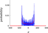
and we confirm the comparison between both sides in Fig. 5 x = 0 𝑥 0 x=0 | γ 0 | = | γ 1 | subscript 𝛾 0 subscript 𝛾 1 |\gamma_{0}|=|\gamma_{1}|
Figure 5: (Color figure online) The blue lines represent the probability distribution ℙ ( X t = x ) ℙ subscript 𝑋 𝑡 𝑥 \mathbb{P}(X_{t}=x) t = 500 𝑡 500 t=500 86 t = 500 𝑡 500 t=500 t 𝑡 t