Multi-Mode Online Knowledge Distillation for Self-Supervised Visual Representation Learning

Abstract

Self-supervised learning (SSL) has made remarkable progress in visual representation learning. Some studies combine SSL with knowledge distillation (SSL-KD) to boost the representation learning performance of small models. In this study, we propose a Multi-mode Online Knowledge Distillation method (MOKD) to boost self-supervised visual representation learning. Different from existing SSL-KD methods that transfer knowledge from a static pre-trained teacher to a student, in MOKD, two different models learn collaboratively in a self-supervised manner. Specifically, MOKD consists of two distillation modes: self-distillation and cross-distillation modes. Among them, self-distillation performs self-supervised learning for each model independently, while cross-distillation realizes knowledge interaction between different models. In cross-distillation, a cross-attention feature search strategy is proposed to enhance the semantic feature alignment between different models. As a result, the two models can absorb knowledge from each other to boost their representation learning performance. Extensive experimental results on different backbones and datasets demonstrate that two heterogeneous models can benefit from MOKD and outperform their independently trained baseline. In addition, MOKD also outperforms existing SSL-KD methods for both the student and teacher models.

1 Introduction

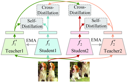
Figure 1: Overview of the proposed Multi-mode Online Knowledge Distillation (MOKD). In MOKD, two different models are trained collaboratively through two types of knowledge distillation modes, i.e., a self-distillation mode and a cross-distillation mode. EMA denotes exponential-moving-average.

Due to the promising performance of unsupervised visual representation learning in many computer vision tasks, self-supervised learning (SSL) has attracted widespread attention from the computer vision community. SSL aims to learn general representations that can be transferred to downstream tasks by utilizing massive unlabeled data.

Among various SSL methods, contrastive learning [21, 8] has shown significant progress in closing the performance gap with supervised methods in recent years. It aims at maximizing the similarity between views from the same instance (positive pairs) while minimizing the similarity among views from different instances (negative pairs). MoCo [21, 10] and SimCLR [8, 9] use both positive and negative pairs for contrast. They significantly improve the performance compared to previous methods [45, 51]. After that, many methods are proposed to solve the limitations in contrastive learning, such as the false negative problem [29, 43, 14, 32, 20], the limitation of large batch size [31, 54], and the problem of hard augmented samples [49, 27]. At the same time, other studies [18, 11, 4, 55, 2, 17, 5] abandon the negative samples during contrastive learning. With relatively large models, such as ResNet50 [23] or larger, these methods achieve comparable performance on different tasks than their supervised counterparts. However, as revealed in previous studies [15, 16], they do not perform well on small models [26, 42] and have a large gap from their supervised counterparts.

To address this challenge in contrastive learning, some studies [44, 9, 1, 37, 15, 58, 16] propose to combine knowledge distillation [24] with contrastive learning (SSL-KD) to improve the performance of small models. These methods first train a larger model in a self-supervised manner and then distill the knowledge of the trained teacher model to a smaller student model. There is a limitation in these SSL-KD methods, i.e., knowledge is distilled to the student model from the static teacher model in a unidirectional way. The teacher model cannot absorb knowledge from the student model to boost its performance.

In this study, we propose a Multi-mode Online Knowledge Distillation method (MOKD), as illustrated in Fig. 1, to boost the representation learning performance of two models simultaneously. Different from existing SSL-KD methods that transfer knowledge from a static pre-trained teacher to a student, in MOKD, two different models learn collaboratively in a self-supervised manner. Specifically, MOKD consists of a self-distillation mode and a cross-distillation mode. Among them, self-distillation performs self-supervised learning for each model independently, while cross-distillation realizes knowledge interaction between different models. In addition, a cross-attention feature search strategy is proposed in cross-distillation to enhance the semantic feature alignment between different models. Extensive experimental results on different backbones and datasets demonstrate that model pairs can both benefit from MOKD and outperform their independently trained baseline. For example, when trained with ResNet [23] and ViT [13], two models can absorb knowledge from each other, and representations of the two models show the characteristics of each other. In addition, MOKD also outperforms existing SSL-KD methods for both the student and teacher models.

The contributions of this study are threefold:

• We propose a novel self-supervised online knowledge distillation method, i.e., MOKD.

• MOKD can boost the performance of two models simultaneously, achieving state-of-the-art contrastive learning performance on different models.

• MOKD achieves state-of-the-art SSL-KD performance.

2 Related Works

2.1 Knowledge Distillation

Knowledge distillation [24] aims to distill knowledge from a larger teacher model to a smaller student model to improve the performance of the student model. Many studies have been proposed in recent years, which can be divided into three groups, i.e., logits-based, feature-based, and relation-based, according to the knowledge types.

Logits-based [24, 36] knowledge distillation utilizes the logits of the teacher model as the knowledge. In the vanilla knowledge distillation [24], the student model mimics the logits of the teacher model by minimizing the KL-divergence of the class distribution. Feature-based methods [40, 39, 7] utilize the output of intermediate layers, i.e., feature maps, as the knowledge to supervise the training of the student model. Relation-based knowledge distillation [38, 59] distills the relation between samples rather than a single instance.

These methods mentioned above perform offline distillation. Some studies [57, 60, 19, 6, 56] are developed to perform online distillation, i.e., the teacher and the student model are trained simultaneously. Deep mutual learning [57] is first proposed to train multiple models collaboratively. After that, studies are proposed to improve deep mutual learning regarding generalization ability [19, 6] and computation efficiency [60]. All these methods are trained in a supervised manner.

2.2 Self-Supervised Knowledge Distillation

Due to significant improvement for small models, knowledge distillation is introduced to self-supervised learning to improve the performance of small models. CRD [44] combines a contrastive loss with knowledge distillation to transfer the structural knowledge of the teacher model. SimCLR-v2 [9] proposes to train a larger model via self-supervised learning first and uses the supervised finetuned large model to distill a smaller model via self-supervised learning. SSKD [52] combines self-supervised learning with supervised learning to transfer richer knowledge. Compress [1] and SEED [15] transfer the knowledge of probability distribution in a self-supervised manner by utilizing the memory bank in MoCo [21]. SimReg [37] directly conducts feature distillation by minimizing the squared Euclidean distance between the features of the teacher and student. While ReKD [58] transfers the relation knowledge to the student. DisCo [16] proposes to transfer the final embeddings of a self-supervised pre-trained teacher. There is a limitation in these SSL-KD methods, i.e., knowledge is distilled to a student model from a static teacher model in a unidirectional way. The teacher model cannot absorb knowledge from the student model. Recently, DoGo [3] and MCL [53] combined MoCo [21] with mutual learning [57] for online SSL-KD. However, they either lack a direct comparison with SSL-KD methods on mainstream backbones and tasks or can’t guarantee the performance of larger models.

3 Methods

In this section, we first introduce the overall architecture of MOKD in Sec. 3.1. Then, the two distillation modes of MOKD, i.e., self-distillation and cross-distillation, are introduced in Sec. 3.2 and Sec. 3.3, respectively. Finally, the training procedure and implementation details are introduced in Sec. 3.4.

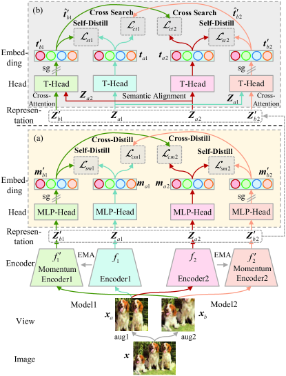
Figure 2: The overall architecture of MOKD. In MOKD, two different models (model1 and model2) are trained collaboratively in a self-supervised manner. There are two types of knowledge distillation modes: self-distillation and cross-distillation modes. And the distillation procedure is performed in two feature spaces projected by two types of projection heads, i.e., (a) MLP-Head and (b) T-Head. “sg" denotes the stop-gradient operation.

3.1 Overall Architecture

The overall architecture of MOKD is shown in Fig. 2. In MOKD, two different models $\mbox{\boldmath$f$}_{i}$ ($i=1,2$) are trained collaboratively in a self-supervised manner. There are two knowledge distillation modes: self-distillation and cross-distillation modes. In each model, a multi-layer-perceptron head (MLP-Head) (Fig. 2(a)) and a Transformer head (T-Head) (Fig. 2(b)) are employed to project the feature representations $Z$ produced by the encoders to the output embeddings $m$ and $t$ for self-distillation and cross-distillation. Here, the T-Head, which consists of several Transformer blocks, is designed to enhance the semantic alignment between the two models. Self-distillation, which is conducted between each model $\mbox{\boldmath$f$}_{i}$ (as a student) and its EMA version model $\mbox{\boldmath$f$}^{\prime}_{i}$ (as a teacher), performs self-supervised learning for each model independently. The self-distillation losses are ${\mathcal{L}_{smi}}$ and ${\mathcal{L}_{sti}}$ for the MLP-Head and T-Head, respectively, which will be introduced in Sec. 3.2. While cross-distillation, which is conducted between the two models, is employed for knowledge interaction between the two models. In cross-distillation, by utilizing the self-attention mechanism of the T-Head, we design a cross-attention feature search strategy to enhance semantic alignment between different models. The cross-distillation losses are ${\mathcal{L}_{cmi}}$ and ${\mathcal{L}_{cti}}$ for the MLP-Head and T-Head, respectively, which will be introduced in Sec. 3.3. Here, the subscript $s$ and $c$ stand for self-distillation and cross-distillation, respectively. And the subscript $m$ and $t$ stand for MLP-Head and T-Head, respectively.

3.2 Self-Distillation

Self-distillation performs the contrastive learning task for each model independently. In this study, we design self-distillation based on the contrastive learning method DINO [5]. Specifically, take the model1 as an example. Given two augmentations ($\mbox{\boldmath$x$}_{a}$ and $\mbox{\boldmath$x$}_{b}$) of an input image $x$, the backbone encoder $f_{1}$ and its EMA version (the momentum encoder $f^{\prime}_{1}$) encode them into the representations: $\mbox{\boldmath$Z$}_{a1}\!=\!f_{1}(\mbox{\boldmath$x$}_{a})$, $\mbox{\boldmath$Z$}^{\prime}_{b1}\!=\!f^{\prime}_{1}(\mbox{\boldmath$x$}_{b})$. The representations are the feature maps (for convolution neural networks (CNN) [23]) or tokens (for vision transformers [13]) before global average pooling. Then, the representations are globally-average-pooled and fed into the corresponding MLP-Head to obtain the final embeddings $\mbox{\boldmath$m$}_{a1}$ and $\mbox{\boldmath$m$}^{\prime}_{b1}$. $\mbox{\boldmath$m$}_{a1}$, $\mbox{\boldmath$m$}^{\prime}_{b1}\in{\mathbb{R}^{K}}$, $K$ is the output dimension. The embeddings are normalized with a softmax function:

$$\mbox{\boldmath$m$}_{a1}^{i}=\frac{{\exp\left({{{\mbox{\boldmath$m$}_{a1}^{i}}\mathord{\left/{\vphantom{{\mbox{\boldmath$m$}_{a1}^{i}}\tau}}\right.\kern-1.2pt}\tau}}\right)}}{{\sum\nolimits_{k=1}^{K}{\exp\left({{{\mbox{\boldmath$m$}_{a1}^{k}}\mathord{\left/{\vphantom{{\mbox{\boldmath$m$}_{a1}^{k}}\tau}}\right.\kern-1.2pt}\tau}}\right)}}}$$ (1)

where $\tau>0$ is a temperature parameter that controls the sharpness of the output distribution. Note that $\mbox{\boldmath$m$}^{\prime}_{b1}$ is also normalized with a similar softmax function with temperature $\tau^{\prime}$. $\mbox{\boldmath$x$}_{a}$ and $\mbox{\boldmath$x$}_{b}$ are fed to the momentum encoder and encoder symmetrically and $\mbox{\boldmath$m$}^{\prime}_{a1}$ and $\mbox{\boldmath$m$}_{b1}$ are obtained respectively. Following DINO [5], the cross-entropy loss is employed as the contrastive loss. This task is a dynamic self-distillation procedure where student (encoder) and teacher (momentum encoder) have the same architecture. Similar self-distillation loss can be calculated for the model2, as follows:

$$\left\{\begin{array}[]{l}{\mathcal{L}_{sm1}}=-\frac{1}{2}\left({\mbox{\boldmath$m$}^{\prime}_{b1}}\log\left({\mbox{\boldmath$m$}_{a1}}\right)+{\mbox{\boldmath$m$}^{\prime}_{a1}}\log\left({\mbox{\boldmath$m$}_{b1}}\right)\right)\\ {\mathcal{L}_{sm2}}=-\frac{1}{2}\left({\mbox{\boldmath$m$}^{\prime}_{b2}}\log\left({\mbox{\boldmath$m$}_{a2}}\right)+{\mbox{\boldmath$m$}^{\prime}_{a2}}\log\left({\mbox{\boldmath$m$}_{b2}}\right)\right)\end{array}\right.$$ (2)

Following DINO [5], we also employ the same whitening strategy to avoid model collapse and multi-crop [4] to enrich augmentations.

As shown in Fig. 2(b), self-distillation is also conducted on the output embeddings $t$ of T-Head to stabilize the training of T-Head. A detailed explanation will be introduced in Sec. 3.3. Specifically, the representations $Z$ are fed into the corresponding T-Head to obtain the final embeddings $t$. $\mbox{\boldmath$t$}\in{\mathbb{R}^{K}}$, $K$ is the output dimension. After the same softmax operation in Eq. 1, the self-distillation loss of T-Head is calculated:

$$\left\{\begin{array}[]{l}{\mathcal{L}_{st1}}=-\frac{1}{2}\left({{{\mbox{\boldmath$t$}^{\prime}}_{b1}}\log\left({{\mbox{\boldmath$t$}_{a1}}}\right)+{{\mbox{\boldmath$t$}^{\prime}}_{a1}}\log\left({{\mbox{\boldmath$t$}_{b1}}}\right)}\right)\\ {\mathcal{L}_{st2}}=-\frac{1}{2}\left({{{\mbox{\boldmath$t$}^{\prime}}_{b2}}\log\left({{\mbox{\boldmath$t$}_{a2}}}\right)+{{\mbox{\boldmath$t$}^{\prime}}_{a2}}\log\left({{\mbox{\boldmath$t$}_{b2}}}\right)}\right)\end{array}\right.$$ (3)

The self-distillation loss for each model is the sum of the self-distillation losses of MLP-Head and T-Head:

$$\left\{\begin{array}[]{l}{\mathcal{L}_{self1}}={\mathcal{L}_{sm1}}+{\mathcal{L}_{st1}}\\ {\mathcal{L}_{self2}}={\mathcal{L}_{sm2}}+{\mathcal{L}_{st2}}\end{array}\right.$$ (4)

3.3 Cross-Distillation

Cross-distillation realizes the interactive learning between two models. We design two interactive learning objectives, i.e., cross-distillation using MLP-Head embedding and cross-distillation using T-Head embedding, to realize the knowledge transfer between two models.

For MLP-Head embedding, it contains rich knowledge of each model. Thus, cross-distillation is conducted between two models to interact knowledge. Specifically, model1 learns knowledge from the momentum version of model2 and vice versa. The cross-distillation can be calculated as follows:

$$\left\{\begin{array}[]{l}{\mathcal{L}_{cm1}}\!=\!-\frac{1}{2}\left({{{\mbox{\boldmath$m$}^{\prime}}_{b2}}\log\left({{\mbox{\boldmath$m$}_{a1}}}\right)\!+\!{{\mbox{\boldmath$m$}^{\prime}}_{a2}}\log\left({{\mbox{\boldmath$m$}_{b1}}}\right)}\right)\\ {\mathcal{L}_{cm2}}\!=\!-\frac{1}{2}\left({{{\mbox{\boldmath$m$}^{\prime}}_{b1}}\log\left({{\mbox{\boldmath$m$}_{a2}}}\right)\!+\!{{\mbox{\boldmath$m$}^{\prime}}_{a1}}\log\left({{\mbox{\boldmath$m$}_{b2}}}\right)}\right)\end{array}\right.$$ (5)

Cross-distillation is conducted between different views and different models (online and another momentum model), which has two advantages. First, cross-distillation between different views can relax the constraint for the same view and is helpful for avoiding the homogenization of two models. Second, cross-distillation between an online model and another momentum model, rather than two online models, provides more stable training since the momentum model is more stable.

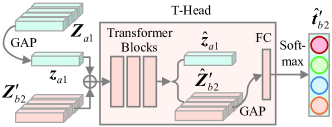
Figure 3: Cross-attention feature search in T-Head. $\oplus$ denotes the concat operation.

During cross-distillation, the knowledge transfer of semantics-relevant features from different views should be enhanced while irrelevant features should be suppressed. To this end, the cross-attention feature search is proposed to search semantics-relevant features from each other for knowledge transfer adaptively. As shown in Fig. 3, the T-Head is designed to apply the self-attention mechanism in Transformer [47] to realize the feature search.

Take the cross-attention feature search between model1 and momentum model2 as an example. We aim to search semantics-relevant features between the feature $\mbox{\boldmath$Z$}_{a1}$ (${\mbox{\boldmath$Z$}_{a1}}\!\in\!{\mathbb{R}^{{N_{1}}\times{C_{1}}}}$, $N_{1}$ denotes the number of local features, which is the product of width and height of feature map for CNN and token number for vision transformer, and $C_{1}$ denotes the dimension of local features) of encoder1 and the feature $\mbox{\boldmath$Z$}^{\prime}_{b2}$ (${\mbox{\boldmath$Z$}^{\prime}_{b2}}\!\in\!{\mathbb{R}^{{N_{2}}\times{C_{2}}}}$, $N_{2}$ and $C_{2}$ denote similar information for encoder2) of momentum encoder2. A global average pooling and a $1\!\times\!1$ convolution operation are conducted on $\mbox{\boldmath$Z$}_{a1}$ to obtain its global feature and unify its dimension with $\mbox{\boldmath$Z$}^{\prime}_{b2}$. Then, the obtained ${\mbox{\boldmath$z$}_{a1}}$ (${z_{a1}}\!\in\!{\mathbb{R}^{{C_{2}}}}$) is concatenated with $\mbox{\boldmath$Z$}^{\prime}_{b2}$ and fed to T-Head:

$$\left[{{{\hat{\mbox{\boldmath$z$}}}_{a1}},{{\hat{\mbox{\boldmath$Z$}}^{\prime}}_{b2}}}\right]={{f^{\prime}}_{t2}}\left({\left[{{\mbox{\boldmath$z$}_{a1}},{{\mbox{\boldmath$Z$}^{\prime}}_{b2}}}\right]}\right)$$ (6)

where ${{f^{\prime}}_{t2}}\left(\cdot\right)$ denotes the function of the transformer blocks in T-Head of momentum model2, and $[\cdot,\cdot]$ refers to the concatenation operation. Through the self-attention mechanism in T-Head, the obtained feature ${\hat{\mbox{\boldmath$Z$}}^{\prime}}_{b2}$ enhances the semantics consistent component while suppressing the irrelevant component with ${\mbox{\boldmath$z$}_{a1}}$. After a global average pooling, an FC layer, and softmax in T-Head, the output embedding ${{{\hat{\mbox{\boldmath$Z$}}^{\prime}}_{b2}}}$ is used for contrast learning with the embedding ${\mbox{\boldmath$t$}_{a1}}$ of ${\mbox{\boldmath$Z$}_{a1}}$. A similar cross-attention feature search procedure is conducted between model2 and momentum model1. The loss for cross-attention feature search can be calculated:

$$\left\{\begin{array}[]{l}{\mathcal{L}_{ct1}}=-\frac{1}{2}({{{\hat{\mbox{\boldmath$t$}}^{\prime}}_{b2}}\log\left({{\mbox{\boldmath$t$}_{a1}}}\right)+{{\hat{\mbox{\boldmath$t$}}^{\prime}}_{a2}}\log\left({{\mbox{\boldmath$t$}_{b1}}}\right)})\\ {\mathcal{L}_{ct2}}=-\frac{1}{2}({{{\hat{\mbox{\boldmath$t$}}^{\prime}}_{b1}}\log\left({{\mbox{\boldmath$t$}_{a2}}}\right)+{{\hat{\mbox{\boldmath$t$}}^{\prime}}_{a1}}\log\left({{\mbox{\boldmath$t$}_{b2}}}\right)})\end{array}\right.$$ (7)

The T-Head of the momentum model cannot be updated if there is only the feature search loss for T-Head. Therefore, self-distillation is also conducted between T-Head embeddings (Eq. 3) to enable the updating of T-Head and provide more stable training. The cross-distillation loss for each model is the sum of the contrastive losses of the MLP-Head and T-Head:

$$\left\{\begin{array}[]{l}{\mathcal{L}_{cross1}}={\mathcal{L}_{cm1}}+{\mathcal{L}_{ct1}}\\ {\mathcal{L}_{cross2}}={\mathcal{L}_{cm2}}+{\mathcal{L}_{ct2}}\end{array}\right.$$ (8)

The overall loss for each model is the weighted sum of self-distillation loss and cross-distillation loss:

$$\left\{\begin{array}[]{l}{\mathcal{L}_{1}}={\mathcal{L}_{self1}}+{\lambda_{1}}{\mathcal{L}_{cross1}}\\ {\mathcal{L}_{2}}={\mathcal{L}_{self2}}+{\lambda_{2}}{\mathcal{L}_{cross2}}\end{array}\right.$$ (9)

where $0\!\leq\!{\lambda_{1}}\!\leq\!1$ and $0\!\leq\!{\lambda_{2}}\!\leq\!1$ are hyper-parameters and denote the weight of the cross-distillation loss of model1 and model2, respectively.

3.4 Implementation Details

Training Procedure. In MOKD, two models are trained cooperatively. Algorithm 1 summarizes the training procedure of MOKD. The SGD and AdamW [35] optimizers are used for CNN and ViT, respectively.

Projection Head. MLP-Head consists of a four-layer MLP with the same architecture as DINO [5]. T-Head consists of 3 transformer blocks with the same architecture as ViT-Small [13] and an FC layer for projection. The output dimension of the two heads is $K\!=\!65536$.

Algorithm 1 PyTorch-Style Pseudocode of MOKD.

⬇

# n1, n1_, n2, n2_: nets and momentum nets

# t1_, t2_: T-Heads of momentum nets

# l: network momentum rates

n1_.params, n2_.params = n1.params, n2.params

for x in loader: # load a minibatch x with n samples

xa, xb = augment(x), augment(x) # random views

# net1 and momentum net1 output

[ma1,ta1,Za1], [mb1,tb1,Zb1] = n1(xa), n1(xb)

[ma1_,ta1_,Za1_], [mb1_,tb1_,Zb1_] = n1_(xa),n1_(xb)

# net2 and momentum net2 output

[ma2,ta2,Za2], [mb2,tb2,Zb2] = n2(xa), n2(xb)

[ma2_,ta2_,Za2_], [mb2_,tb2_,Zb2_] = n2_(xa),n2_(xb)

# cross-attention feature search

tb1_s, ta1_s = t1_(Za2, Zb1_), t1_(Zb2, Za1_)

tb2_s, ta2_s = t2_(Za1, Zb2_), t2_(Zb1, Za2_)

# self-distillation loss

loss_sm1 = H(mb1_,ma1)/2 + H(ma1_,mb1)/2

loss_sm2 = H(mb2_,ma2)/2 + H(ma2_,mb2)/2

loss_st1 = H(tb1_,ta1)/2 + H(ta1_,tb1)/2

loss_st2 = H(tb2_,ta2)/2 + H(ta2_,tb2)/2

# cross-distillation loss

loss_cm1 = H(mb2_,ma1)/2 + H(ma2_,mb1)/2

loss_cm2 = H(mb1_,ma2)/2 + H(ma1_,mb2)/2

loss_it1 = H(tb2_s,ta1)/2 + H(ta2_s,tb1)/2

loss_it2 = H(tb1_s,ta2)/2 + H(ta1_s,tb2)/2

# total loss

loss1 = (loss_sm1 + loss_st1) + lamda1 * (loss_cm1 + loss_ct1)

loss2 = (loss_sm2 + loss_st2) + lamda2 * (loss_cm2 + loss_ct2)

# back-propagate

loss1.backward(), loss2.backward()

# nets update

update(n1), update(n2)

n1_.params = l*n1.params + (1-l)*n1.params

n2_.params = l*n2.params + (1-l)*n2.params

def H(t, s):

return - (t * log(s)).sum(dim=1).mean()

4 Experiments

In this section, we conduct comprehensive experiments to evaluate the effectiveness of MOKD. Different sizes of CNNs and vision transformers are used as encoders. Heterogeneous and homogeneous models are evaluated. For heterogeneous MOKD, a ResNet [23] and a ViT [13] are used. Specifically, ResNet101 (R101)/ResNet50 (R50) is used for CNN, and ViT-Base (ViT-B)/ViT-Small (ViT-S) is used for vision transformer. For homogeneous MOKD, two CNNs or two ViTs are used. For two CNNs, R101/R50 is used for the larger model, ResNet34 (R34)/ResNet18 (R18) is used for the smaller model. For two ViTs, ViT-S and ViT-Tiny (ViT-T) are used. In addition, we also conduct experiments for two models have the same architecture, including R50, R18, and ViT-S. All models are trained on the ImageNet [41] training set. Without a specific statement, the default setting is 256 batch size and 100 epochs. We follow most hyper-parameters settings of DINO [5]. More details for experiments can be found in Supplementary Material.

4.1 Experiments on ImageNet

After pre-training, the $k$-NN and linear probing are employed to evaluate the representation performance. For linear probing, a linear classifier added to the frozen backbone is trained for 100 epochs [21]. The top-1 accuracy on the validation set is adopted as the evaluation metric.

$k$-NN and Linear Probing Accuracy. MOKD is compared with the baseline which two models are trained independently using DINO [5]. The results are shown in Tab. 1. For heterogeneous models (ResNet-ViT), MOKD significantly improves the performance of two models compared with models that are trained independently. For example, with R50-ViT-B, the linear probing accuracy of the two models improves by 3.5% (from 72.1% to 75.6%) and 1.0% (from 77.0% to 78.0%), respectively. With homogeneous models (two ResNets and two ViTs), MOKD improves the performance of the smaller model with a large margin. The experimental results demonstrate that MOKD can effectively transfer knowledge between different models to boost the representation performance.

		$k$-NN				Linear Probing
Backbone		Independent		MOKD		Independent		MOKD
Net1	Net2	Net1	Net2	Net1	Net2	Net1	Net2	Net1	Net2
R50	ViT-S	62.8	69.9	67.1	70.8	72.1	73.8	74.1	74.4
R50	ViT-B	62.8	73.6	70.6	75.2	72.1	77.0	75.6	78.0
R101	ViT-S	66.9	69.9	68.3	70.7	74.6	73.8	75.0	74.7
R101	ViT-B	66.9	73.6	68.5	74.7	74.6	77.0	75.2	77.5
R50	R34	62.8	60.6	62.9	61.2	72.1	66.5	72.3	67.0
R50	R18	62.8	53.2	62.7	57.1	72.1	61.2	72.0	63.4
R101	R34	66.9	60.6	66.9	61.7	74.6	66.5	74.7	67.6
R101	R18	66.9	53.2	66.7	57.4	74.6	61.2	74.5	63.6
R50	R50	62.8	62.8	63.0	63.1	72.1	72.1	72.4	72.4
R18	R18	53.2	53.2	53.4	53.4	61.2	61.2	61.3	61.4
ViT-S	ViT-T	69.9	59.9	70.6	62.1	73.8	63.8	74.2	64.3
ViT-S	ViT-S	69.9	69.9	70.5	70.4	73.8	73.8	74.3	74.2

Table 1: $k$-NN and linear probing accuracy (%) on ImageNet.

Compared with SSL Methods. The performance of MOKD for different models is compared with other outstanding SSL methods. Most contrastive learning methods conduct experiments using R50, and several methods use ViT-S and ViT-B. Thus, we compare the performance of the three models. As shown in Tab. 2, MOKD achieves the best performance for R50, ViT-S, and ViT-B.

Method	Backbone	BS	Epoch	$k$-NN	LP
SimCLR [8]	R50	4096	1000	-	69.3
BYOL [18]	R50	4096	1000	66.9	74.3
SwAV [4]	R50	4096	800	-	75.3
MoCo-v2 [10]	R50	256	200	55.6	67.5
SimSiam [11]	R50	256	200	-	70.0
MSF [29]	R50	256	200	64.9	72.4
NNCLR [14]	R50	4096	200	-	70.7
Triplet [48]	R50	832	200	-	74.1
Barlow Twins [55]	R50	2048	1000	-	73.2
OBoW [17]	R50	256	200	-	73.8
AdCo [27]	R50	256	200	-	73.2
MoCo-v3 [12]	R50	4096	300	-	72.8
UniVIP [32]	R50	4096	200	-	73.1
HCSC [20]	R50	256	200	-	73.3
DINO [5]	R50	4080	800	67.5	75.3
MOKD (R50-ViT-B)	R50	256	100	70.6	75.6
SimCLR [8]	ViT-S	4096	300	-	69.0
BYOL [18]	ViT-S	1024	300	66.6	71.4
SwAV [4]	ViT-S	1024	300	64.7	71.8
MoCo-v3 [12]	ViT-S	4096	300	-	72.5
DINO [5]	ViT-S	256	100	69.9	73.8
DINO [5]	ViT-S	256	200	72.8	75.9
MOKD (R50-ViT-S)	ViT-S	256	100	70.8	74.4
MOKD (R50-ViT-S)	ViT-S	256	200	73.1	76.3
MoCo-v3 [12]	ViT-B	4096	300	-	76.5
DINO [5]	ViT-B	256	100	73.6	77.0
DINO [5]	ViT-B	256	200	75.1	77.7
MOKD (R50-ViT-B)	ViT-B	256	100	75.2	78.0
MOKD (R50-ViT-B)	ViT-B	256	200	76.0	78.4

Table 2: Comparison of MOKD and SSL methods on ImageNet using $k$-NN and linear probing (LP) accuracy. Bold font indicates the best results. BS denotes batch size.

Method	R50	R34	R50	R18	R101	R34	R101	R18
Supervised	76.2	75.0	76.2	72.1	77.0	75.0	77.0	72.1
SEED [15]	67.4	58.5	67.4	57.6	70.3	61.6	70.3	58.9
ReKD [58]	-	-	67.6	59.6	-	-	69.7	59.7
MCL [53]	61.8	55.0	59.5	51.4	62.8	55.6	60.8	51.8
DisCo [16]	67.4	62.5	67.4	60.6	69.1	64.4	69.1	62.3
MOKD	72.3	67.0	72.0	63.4	74.7	67.6	74.5	63.6

Table 3: Comparison of MOKD and SSL-KD methods on ImageNet using the linear probing accuracy.

Compared with SSL-KD Methods. MOKD is also compared with other SSL-KD methods, including SEED[15], ReKD[58], MCL[53], and DisCo[16]. Following SEED and DisCo, R101 and R50 are used as the larger model (or teacher model), and R34 and R18 are employed as the smaller model (or student model). The linear probing accuracy is reported. The results are shown in Tab. 3. MOKD achieves the best performance for all models, outperforming the state-of-the-art method DisCo. For example, with R50-R34, MOKD achieves 67.0% for R34, which outperforms DisCo by a margin of 4.5%.

4.2 Semi-Supervised Learning

In this part, we evaluate the performance of MOKD under the semi-supervised setting. Specifically, we use the 1% and 10% subsets [9] of the ImageNet [41] training set for fine-tuning, which follows the semi-supervised protocol in [8]. Models are fine-tuned with 1024 batch size for 60 epochs and 30 epochs on 1% and 10% subsets, respectively. The top-1 accuracy is employed. The results are reported in Tab. 4. Fine-tuning using 1% and 10% training data, MOKD improves the performance of the two models with a large margin compared with the models pre-trained independently.

		1%				10%
Backbone		Independent		MOKD		Independent		MOKD
Net1	Net2	Net1	Net2	Net1	Net2	Net1	Net2	Net1	Net2
R50	ViT-S	49.5	44.6	53.8	44.9	67.3	67.8	68.7	68.2
R50	ViT-B	49.5	57.1	57.2	58.3	67.3	73.4	70.2	74.3
R101	ViT-S	54.8	44.6	56.9	44.8	70.7	67.8	71.0	68.8
R101	ViT-B	54.8	57.1	57.1	63.9	70.7	73.4	71.0	74.7
R50	R34	49.5	44.5	49.8	46.1	67.3	62.9	67.3	63.5
R50	R18	49.5	35.8	50.0	40.8	67.3	56.0	67.3	56.7
R101	R34	54.8	44.5	54.8	47.0	70.7	62.9	70.8	63.7
R101	R18	54.8	35.8	54.9	41.4	70.7	56.0	70.7	56.8
R50	R50	49.5	49.5	50.1	49.8	67.3	67.3	67.6	67.4
R18	R18	35.8	35.8	36.5	36.4	56.0	56.0	56.3	56.3
ViT-S	ViT-T	44.6	19.2	44.9	20.0	67.8	55.2	68.2	55.8
ViT-S	ViT-S	44.6	44.6	44.8	44.7	67.8	67.8	68.3	68.3

Table 4: Semi-supervised learning on ImageNet subset. The top-1 accuracy is reported.

4.3 Transfer to Cifar10/Cifar100

We further fine-tune the pre-trained models on Cifar10 and Cifar100 [30] datasets to analyze the generalization of representations obtained by MOKD. The models are fine-tuned with 1024 batch size for 100 epochs. The top-1 accuracy is employed. As shown in Tab. 5, MOKD surpasses the independently pre-training baseline with different models on both Cifar10 and Cifar100. This experiment shows the good generalization ability of MOKD.

		Cifar10				Cifar100
Backbone		Independent		MOKD		Independent		MOKD
Net1	Net2	Net1	Net2	Net1	Net2	Net1	Net2	Net1	Net2
R50	ViT-S	97.3	98.6	97.6	98.7	85.3	88.8	86.2	88.9
R50	ViT-B	97.3	98.8	97.6	99.2	85.3	91.0	85.6	91.3
R101	ViT-S	98.2	98.6	98.4	98.8	87.6	88.8	87.8	89.0
R101	ViT-B	98.2	98.8	98.3	99.0	87.6	91.0	87.8	91.4
R50	R34	97.3	97.0	97.5	97.2	85.3	83.3	85.0	83.7
R50	R18	97.3	95.6	97.5	96.1	85.3	80.2	85.2	81.1
R101	R34	98.2	97.0	98.3	97.3	87.6	83.3	87.6	83.9
R101	R18	98.2	95.6	98.1	96.0	87.6	80.2	87.3	80.8
R50	R50	97.3	97.3	97.7	97.6	85.3	85.3	85.6	85.4
R18	R18	95.6	95.6	95.9	95.8	80.2	80.2	80.6	80.6
ViT-S	ViT-T	98.6	97.2	98.7	97.4	88.8	84.1	89.0	84.4
ViT-S	ViT-S	98.6	98.6	98.7	98.7	88.8	88.8	89.0	88.9

Table 5: Tranfer learning on Cifar10 and Cifar100. The top-1 accuracy is reported.

4.4 Transfer to Detection and Segmentation

In this part, we evaluate the representation of MOKD on dense prediction tasks, i.e., object detection and instance segmentation, on MS COCO [33] datasets. We use the train2017 set for training and evaluate on the val2017 set. Following [15], C4-based Mask R-CNN [22] is used for objection detection and instance segmentation on COCO. And R34 is used as backbone, which is initialized by the pre-trained models. Our implementation is based on detectron2 [50]. The experimental results are shown in Tab. 6. It can be seen that MOKD achieves the best performance, which demonstrates that MOKD has good generalization ability on dense prediction tasks.

Method	Net1	Net2	Detection			Segmentation
			$\rm{AP}^{\rm{b}}$	$\rm{AP}_{50}^{\rm{b}}$	$\rm{AP}_{75}^{\rm{b}}$	$\rm{AP}^{\rm{s}}$	$\rm{AP}_{50}^{\rm{s}}$	$\rm{AP}_{75}^{\rm{s}}$
MoCov2 [10]	-	R34	38.1	56.8	40.7	33.0	53.2	35.3
DINO [5]	-	R34	39.6	58.6	42.5	34.2	55.3	36.4
SEED [15]	R50	R34	38.4	57.0	41.0	33.3	53.2	35.3
MCL [53]	R50	R34	39.5	58.4	42.5	34.1	55.3	36.4
DisCo [16]	R50	R34	40.0	59.1	43.4	34.9	56.3	37.1
MOKD	R50	R34	40.3	59.7	43.7	34.9	56.5	37.1
SEED [15]	R101	R34	38.5	57.3	41.4	33.6	54.1	35.6
MCL [53]	R101	R34	39.2	58.2	42.1	33.8	54.9	35.7
DisCo [16]	R101	R34	40.0	59.1	43.2	34.7	55.9	37.4
MOKD	R101	R34	40.3	59.3	43.5	34.8	56.2	36.9

Table 6: Object detection and instance segmentation on COCO with R34 as backbone. C4-based Mask R-CNN [22] is adopted as the detector.

4.5 Ablation Study

In this section, we analyze the influence of each component in MOKD. The ImageNet100 dataset, which contains 100 randomly selected categories from ImageNet, is adopted to speed up the training time. All models are trained on the ImageNet100 training set with 256 batch size and 200 epochs and tested on the validation set. The linear probing top-1 accuracy is employed as the evaluation metric.

Effectiveness of Each Loss Term. There are four loss terms for each model in MOKD, i.e., $\mathcal{L}_{sm}$, $\mathcal{L}_{st}$, $\mathcal{L}_{cm}$, and $\mathcal{L}_{ct}$ in Eq. 2, Eq. 3, Eq. 5, and Eq. 7, respectively. We use R50-ViT-S to analyze the influence of each loss term. The results are shown in Tab. 7. Note that the result with only $\mathcal{L}_{sm}$ is the DINO [5] baseline that trains the two models independently. With the addition of $\mathcal{L}_{cm}$, $\mathcal{L}_{st}$, and $\mathcal{L}_{ct}$, the performance improves gradually, which indicates that self-distillation and cross-distillation of MLP-head and T-Head can benefit the representation performance of MOKD.

$\mathcal{L}_{sm}$	$\mathcal{L}_{cm}$	$\mathcal{L}_{st}$	$\mathcal{L}_{ct}$	R50	ViT-S
$\checkmark$				87.0	80.3
$\checkmark$	$\checkmark$			87.2	82.6
$\checkmark$	$\checkmark$	$\checkmark$		87.7	83.5
$\checkmark$	$\checkmark$	$\checkmark$	$\checkmark$	88.3	84.6

Table 7: Influence of each loss term.

Influence of $\lambda_{1}$ and $\lambda_{2}$. $\lambda_{1}$ and $\lambda_{2}$ in Eq. 9 are the weights of cross-distillation loss of model1 and model2, respectively. Tab. 8 shows the results. As shown in the first row, when $\lambda_{2}\!=\!1$ for ViT-S, the performance of R50 get worse with the increase of $\lambda_{1}$, which indicates that it is better to set a small value for the model with better performance. When $\lambda_{1}\!=\!0$, R50 is trained without cross-distillation and achieves insignificant improvement, which indicates that cross-distillation is essential for the model with better performance. As shown in the third row, when $\lambda_{1}\!=\!0.1$ for R50, the performance of ViT-S improves with the increase of $\lambda_{2}$, which demonstrates that paying more emphasis on cross-distillation is beneficial to the model with inferior performance. In this study, $\lambda_{1}$ and $\lambda_{2}$ are set to 1 and 0.1 for the larger and smaller models, respectively. While for model pairs with the same backbone, $\lambda_{1}$ and $\lambda_{2}$ are both set to 1.

$\lambda_{1}$, $\lambda_{2}$	0, 1	0.1, 1	0.5, 1	1, 1
R50, ViT-S	87.2, 83.1	88.3, 84.6	87.9, 84.5	87.4, 84.1
$\lambda_{1}$, $\lambda_{2}$	0.1, 0	0.1, 0.1	0.1, 0.5	0.1, 1
R50, ViT-S	87.4, 80.4	87.5, 81.3	87.9, 83.1	88.3, 84.6

Table 8: Influence of cross-distillation loss weights.

Methods	Independent	MOKD	Independent
$k$-NN	62.8, 69.9	67.1, 70.8	67.5, 70.8
Consistency	0.871	0.901	0.900

Table 9: Prediction consistency between two models.

4.6 Visualization and Analysis

Does MOKD Make Models More Similar? In this part, we analyze the representations learned by MOKD. First, we analyze if representations of two models trained by MOKD tend to be more similar. To this end, the fraction of samples that two model pairs make the same prediction is calculated. The R50-ViT-S configuration, which is pre-trained on ImageNet, is employed, and $k$-NN is applied on ImageNet100. As shown in Tab. 9, the prediction consistency rate of MOKD increases compared to the result of independent training in the second column. However, this increase is mainly caused by the performance improvement of the two models compared to the consistency rate in the last column, which is obtained by replacing the R50 model trained by MOKD with an R50 model with relative accuracy trained by DINO. The results verify that there is no significant tendency for representations of two models trained by MOKD to become more similar. Fig. 4 visualizes the feature distributions of the two models trained by MOKD. The two models show different feature distributions, which further verifies that MOKD does not make models more similar. More results can be found in Fig. S1 in Supplementary Material.

What Knowledge Is Learned in MOKD? We investigate the characteristic of features on each layer to analyze the difference between models trained independently and trained by MOKD. Specifically, we calculate the mean attention distance (MAD) [13] for ViT models. For CNN models, a similar average distance can also be calculated on the feature map based on its self-attention weights. As shown in Fig. 5(a)(b), we found that the MAD on deep layers (layer 10-12) of the ViT-S model trained by MOKD (with R50) decreased compared to those of the ViT-S model trained independently, which indicates that the ViT-S model trained by MOKD turns to be more “local" on deep layers. The opposite phenomenon can be seen on ResNets. As shown in Fig. 5(c)(d), the MAD on each layer of ResNet models trained by MOKD (with ViTs) increase compared to those of ResNet models trained independently, which indicates that ResNet models trained by MOKD (with ViTs) turn to be more “global". However, this phenomenon is not shown in two ResNet models trained by MOKD. That is, through MOKD, two heterogeneous models absorb knowledge from each other, i.e., ViT model learns more locality while CNN model learns more global information. More results can be found in Fig. S2 in Supplementary Material.

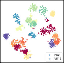
(a) Independent (R50-ViT-S).

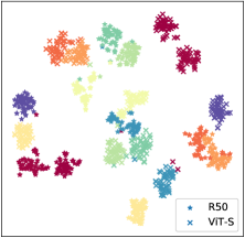
(b) MOKD (R50-ViT-S).

Figure 4: T-SNE [46] visualization of feature distributions on ImageNet100. Ten categories (shown in different colors) are randomly selected for better visualization.

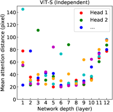
(a) ViT-S trained independently.

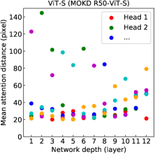
(b) ViT-S trained by MOKD.

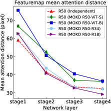
(c) R50 models.

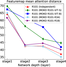
(d) R101 models.

Figure 5: Mean attention distances [13] of different models.

5 Conclusions

In this study, we propose the MOKD method, where two different models learn collaboratively through self-distillation and cross-distillation in a self-supervised manner. Extensive experiments on different backbones and tasks demonstrate that MOKD can boost the feature representation performance of different models. It achieves state-of-the-art performance for self-supervised knowledge distillation. We hope this study could inspire boosting representation learning performance via knowledge interaction between heterogeneous models.

As an online knowledge distillation method, the main limitation of MOKD is that the larger model needs to be repeatedly trained for different smaller models, which requires more computation cost than offline knowledge distillation. How to design an efficient MOKD can be further studied. For example, introducing efficient fine-tuning methods [25, 28] into MOKD may be a possible future study to realize efficient MOKD.

Supplementary Material

The implementation details are introduced first. Then we show more visualization results for the feature distributions shown in Fig. 4 and mean attention distances shown in Fig. 5. Finally, we present more experimental results.

A Implementation Details

A.1 Pre-training on ImageNet

Data Augmentation. The data augmentations consist of random cropping (with a scale of 0.25-1.0), resizing to $224\times 224$, random horizontal flip, gaussian blur, and color jittering. The local augmentations for the multi-crop strategy consist of random cropping (with a scale of 0.05-0.25), resizing to $96\times 96$, random horizontal flip, gaussian blur, and color jittering. Two global views and eight local views are used in all pre-taining experiments.

Training. During the pre-training procedure, we follow the most hyper-parameters setting of DINO [5]. Without a specific statement, the default batch size is 256. The SGD and AdamW [35] optimizers are used for ResNet and ViT, respectively. The learning rate is linearly warmed up to its base value during the first 10 epochs. And the base learning rate is set to $0.1$ and $0.0003$ for ResNet and ViT, respectively. After the warm-up procedure, the learning rate is decayed with a cosine schedule [34]. The weight decay is set to $1e-4$ and $0.04$ for ResNet and ViT, respectively. For the temperatures, $\tau$ is set to $0.1$, and a linear warm-up from $0.04$ to $0.07$ is set to $\tau^{\prime}$ during the first 30 epochs. Following DINO [5], the centering operation is applied to the output of the momentum encoders to avoid collapse. $\lambda_{1}$ and $\lambda_{2}$ in Eq. (9) are set to 1 and 0.1 for the larger and smaller models, respectively. While for model pairs with the same backbone, $\lambda_{1}$ and $\lambda_{2}$ are set to 1.

A.2 $k$-NN and Linear Probing on ImageNet

After pre-training, the $k$-NN and linear probing are employed to evaluate the representation performance. For $k$-NN, it is implemented based on DINO [5]. We report the best result among $k=10,20,100,200$.

For linear probing, a linear classifier added to the frozen backbone is trained [21]. The linear classifier is trained with the SGD optimizer and a batch size of $2048$ for $100$ epochs on the ImageNet training set. The learning rate is linearly warmed up to its base value during the first 10 epochs. And the base learning rate is set to $0.08$ and $0.008$ for ResNet and ViT, respectively. After the warm-up stage, the learning rate is decayed with a cosine schedule [34]. Weight decay is not used. The input resolution is $224\times 224$ during training and testing.

A.3 Semi-Supervised Learning on ImageNet

We use the 1% and 10% subsets of the ImageNet [41] training set for fine-tuning, which follows the semi-supervised protocol in [8]. The same splits of 1% and 10% of ImageNet training set in [9] are used. Models are fine-tuned with 1024 batch size for 60 epochs and 30 epochs on 1% and 10% subsets, respectively. The SGD optimizer is adopted. The learning rate is linearly warmed up to its base value during the first 5 epochs. And the best base learning rate is searched for each model. After the warm-up procedure, the learning rate is decayed with a cosine schedule [34]. The input resolution is $224\times 224$ during training and testing.

A.4 Fine-tuning on Cifar10/Cifar100

Most settings keep the same with the experiments of semi-supervised learning on ImageNet except for the training epochs. On Cifar10/100, the warming-up epoch is set to 10, and the training epoch is set to 100.

A.5 Fine-tuning on COCO

Following [15], The C4-based Mask R-CNN [22] detector is used for objection detection and instance segmentation on COCO. The model is trained for 180k iterations, i.e., the 2$\times$ schedule. The SGD optimizer is adopted. The initial learning rate is set to 0.02. The scale of images for training is set as [600, 800] and 800 at inference. We report $\rm{AP}^{\rm{b}}$, $\rm{AP}_{50}^{\rm{b}}$, and $\rm{AP}_{75}^{\rm{b}}$ for object detection and $\rm{AP}^{\rm{s}}$, $\rm{AP}_{50}^{\rm{s}}$, and $\rm{AP}_{75}^{\rm{s}}$ for instance segmentation.

B More Visualizations

B.1 T-SNE Visualization of Feature Distribution

Following Fig. 4, more model pairs, including two ResNets and two ViTs are visualized. As shown in Fig. S1, the model pairs (R50-R34 and ViT-S-ViT-T) trained by MOKD also show different feature distributions, demonstrating that MOKD does not make models more similar. In addition, we can see that the feature distributions of R34 and ViT-T get better when trained with MOKD.

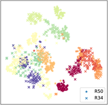
(a) Independent (R50-R34).

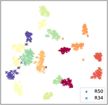
(b) MOKD (R50-R34).

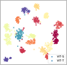
(c) Independent (ViT-S-ViT-T).

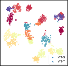
(d) MOKD (ViT-S-ViT-T).

Figure S1: T-SNE [46] visualization of feature distributions on ImageNet100. Ten categories (shown in different colors) are randomly selected for better visualization. Different color denotes different category and different marker denotes different model.

(a) ViT-S (Independent).

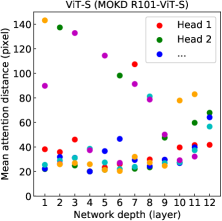
(b) ViT-S (MOKD with R101).

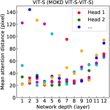
(c) ViT-S (MOKD with ViT-S).

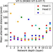
(d) ViT-S (MOKD with ViT-T).

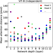
(e) ViT-B (Independent).

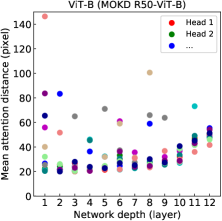
(f) ViT-B (MOKD with R50).

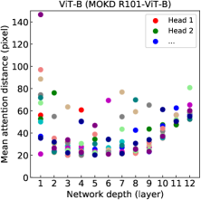
(g) ViT-B (MOKD with R101).

Figure S2: Mean attention distances [13] of different models.

B.2 Mean Attention Distances

In Fig. 5, we show the mean attention distances [13] of ViT-S, R50, and R101 trained independently (by DINO) and trained by MOKD. For ResNets, when trained with ViTs, i.e., R50-ViT-S, R5O-ViT-B, R101-ViT-S, and R101-ViT-B, the ResNet models trained by MOKD turns to be more “global". However, this phenomenon is not shown in two ResNet model pairs trained by MOKD, i.e., R50-R34, R50-R18, R101-R34, and R101-R18. As shown in Fig. S2, we show more mean attention distances of ViTs. Compared with the ViT models trained independently (as shown in Fig. S2(a)(e)), the mean attention distances on deep layers (layer 10-12) of the ViT models trained with ResNet models (as shown in Fig. S2(b)(f)(g)) decrease, which indicates that the ViT-S model trained by MOKD turns to be more “local" on deep layers. This phenomenon is not shown in two ViT models trained by MOKD, as shown in Fig. S2(c)(d). These observations show that two heterogeneous models absorb knowledge from each other: ViT model learns more locality while CNN model learns more global information.

C More Experiments

C.1 Results on Other Convnets

We conduct experiments on EfficientNet-B0 [42] and MobileNet-v3-Large [26]. Following DisCo [16], R50 and R101 are selected as the larger models. We pre-train MOKD with 256 batch size for 100 epochs on ImageNet. As shown in Tab. S1, MOKD brings consistent improvements over different model pairs. It achieves the best performance for EfficientNet-B0 [42] and MobileNet-v3-Large [26].

C.2 Influence of T-Head Depth

T-Head is added for cross-attention feature search in MOKD. As shown in Tab. S2, increasing T-Head depth (number of transformer blocks) improves the performance of MOKD. However, extra computation costs brought by T-Head should be controlled. Thus, T-Head depth should be small and set to 3 in this study.

Method	R50	Eff-b0	R50	Mob-v3	R101	Eff-b0	R101	Mob-v3
SEED [15]	67.4	61.3	67.4	55.2	70.3	63.0	70.3	59.9
ReKD [58]	67.6	63.4	67.6	56.7	69.7	65.0	69.7	59.6
DisCo [16]	67.4	66.5	67.4	64.4	69.1	68.9	69.1	65.7
MOKD	72.5	69.2	72.2	66.0	74.9	70.1	74.7	67.2

Table S1: Results on other convnets.

Depth	1	2	3
R50, ViT-S	87.4, 83.3	88.1, 84.1	88.3, 84.6

Table S2: Influence of T-Head depth.

C.3 Training Time and Memory Requirement

We show the total training time and peak memory per GPU (“mem.”) when training ViT-S model pairs on an 8 V100 GPU machine. We pre-train DINO [5] and MOKD with 256 batch size for 100 epochs on ImageNet. From Tab. S3, we can tell that the total memory requirement and training time of training two models independently via DINO [5] are comparable to those of MOKD.

Method	Backbones	Time (h)	Mem.(G)	LP
DINO [5]	R50/ViT-S	97+94	6.4+6.3	72.1/73.8
MOKD	R50-ViT-S	122	13.5	74.1/74.4

Table S3: Training Time and Memory Requirement.

References

- [1] Soroush Abbasi Koohpayegani, Ajinkya Tejankar, and Hamed Pirsiavash. Compress: Self-supervised learning by compressing representations. NeurIPS, 33:12980–12992, 2020.
- [2] Adrien Bardes, Jean Ponce, and Yann LeCun. Vicreg: Variance-invariance-covariance regularization for self-supervised learning. arXiv preprint arXiv:2105.04906, 2021.
- [3] Prashant Bhat, Elahe Arani, and Bahram Zonooz. Distill on the go: Online knowledge distillation in self-supervised learning. In CVPRW, pages 2678–2687, 2021.
- [4] Mathilde Caron, Ishan Misra, Julien Mairal, Priya Goyal, Piotr Bojanowski, and Armand Joulin. Unsupervised learning of visual features by contrasting cluster assignments. NeurIPS, 33:9912–9924, 2020.
- [5] Mathilde Caron, Hugo Touvron, Ishan Misra, Hervé Jégou, Julien Mairal, Piotr Bojanowski, and Armand Joulin. Emerging properties in self-supervised vision transformers. In ICCV, pages 9650–9660, 2021.
- [6] Defang Chen, Jian-Ping Mei, Can Wang, Yan Feng, and Chun Chen. Online knowledge distillation with diverse peers. In AAAI, volume 34, pages 3430–3437, 2020.
- [7] Defang Chen, Jian-Ping Mei, Yuan Zhang, Can Wang, Zhe Wang, Yan Feng, and Chun Chen. Cross-layer distillation with semantic calibration. In AAAI, volume 35, pages 7028–7036, 2021.
- [8] Ting Chen, Simon Kornblith, Mohammad Norouzi, and Geoffrey Hinton. A simple framework for contrastive learning of visual representations. In International conference on machine learning, pages 1597–1607. PMLR, 2020.
- [9] Ting Chen, Simon Kornblith, Kevin Swersky, Mohammad Norouzi, and Geoffrey E Hinton. Big self-supervised models are strong semi-supervised learners. NeurIPS, 33:22243–22255, 2020.
- [10] Xinlei Chen, Haoqi Fan, Ross Girshick, and Kaiming He. Improved baselines with momentum contrastive learning. arXiv preprint arXiv:2003.04297, 2020.
- [11] Xinlei Chen and Kaiming He. Exploring simple siamese representation learning. In CVPR, pages 15750–15758, 2021.
- [12] Xinlei Chen, Saining Xie, and Kaiming He. An empirical study of training self-supervised vision transformers. In ICCV, pages 9640–9649, 2021.
- [13] Alexey Dosovitskiy, Lucas Beyer, Alexander Kolesnikov, Dirk Weissenborn, Xiaohua Zhai, Thomas Unterthiner, Mostafa Dehghani, Matthias Minderer, Georg Heigold, Sylvain Gelly, et al. An image is worth 16x16 words: Transformers for image recognition at scale. ICLR, 2021.
- [14] Debidatta Dwibedi, Yusuf Aytar, Jonathan Tompson, Pierre Sermanet, and Andrew Zisserman. With a little help from my friends: Nearest-neighbor contrastive learning of visual representations. In ICCV, pages 9588–9597, 2021.
- [15] Zhiyuan Fang, Jianfeng Wang, Lijuan Wang, Lei Zhang, Yezhou Yang, and Zicheng Liu. Seed: Self-supervised distillation for visual representation. ICLR, 2021.
- [16] Yuting Gao, Jia-Xin Zhuang, Ke Li, Hao Cheng, Xiaowei Guo, Feiyue Huang, Rongrong Ji, and Xing Sun. Disco: Remedy self-supervised learning on lightweight models with distilled contrastive learning. ECCV, 2022.
- [17] Spyros Gidaris, Andrei Bursuc, Gilles Puy, Nikos Komodakis, Matthieu Cord, and Patrick Perez. Obow: Online bag-of-visual-words generation for self-supervised learning. In CVPR, pages 6830–6840, 2021.
- [18] Jean-Bastien Grill, Florian Strub, Florent Altché, Corentin Tallec, Pierre Richemond, Elena Buchatskaya, Carl Doersch, Bernardo Avila Pires, Zhaohan Guo, Mohammad Gheshlaghi Azar, et al. Bootstrap your own latent-a new approach to self-supervised learning. NeurIPS, 33:21271–21284, 2020.
- [19] Qiushan Guo, Xinjiang Wang, Yichao Wu, Zhipeng Yu, Ding Liang, Xiaolin Hu, and Ping Luo. Online knowledge distillation via collaborative learning. In CVPR, pages 11020–11029, 2020.
- [20] Yuanfan Guo, Minghao Xu, Jiawen Li, Bingbing Ni, Xuanyu Zhu, Zhenbang Sun, and Yi Xu. Hcsc: Hierarchical contrastive selective coding. In CVPR, pages 9706–9715, 2022.
- [21] Kaiming He, Haoqi Fan, Yuxin Wu, Saining Xie, and Ross Girshick. Momentum contrast for unsupervised visual representation learning. In CVPR, pages 9729–9738, 2020.
- [22] Kaiming He, Georgia Gkioxari, Piotr Dollár, and Ross Girshick. Mask r-cnn. In ICCV, pages 2961–2969, 2017.
- [23] Kaiming He, Xiangyu Zhang, Shaoqing Ren, and Jian Sun. Deep residual learning for image recognition. In CVPR, pages 770–778, 2016.
- [24] Geoffrey Hinton, Oriol Vinyals, Jeff Dean, et al. Distilling the knowledge in a neural network. Advances in Neural Information Processing Systems Workshop, 2(7), 2015.
- [25] Neil Houlsby, Andrei Giurgiu, Stanislaw Jastrzebski, Bruna Morrone, Quentin De Laroussilhe, Andrea Gesmundo, Mona Attariyan, and Sylvain Gelly. Parameter-efficient transfer learning for nlp. In ICML, pages 2790–2799. PMLR, 2019.
- [26] Andrew Howard, Mark Sandler, Grace Chu, Liang-Chieh Chen, Bo Chen, Mingxing Tan, Weijun Wang, Yukun Zhu, Ruoming Pang, Vijay Vasudevan, et al. Searching for mobilenetv3. In ICCV, pages 1314–1324, 2019.
- [27] Qianjiang Hu, Xiao Wang, Wei Hu, and Guo-Jun Qi. Adco: Adversarial contrast for efficient learning of unsupervised representations from self-trained negative adversaries. In CVPR, pages 1074–1083, 2021.
- [28] Menglin Jia, Luming Tang, Bor-Chun Chen, Claire Cardie, Serge Belongie, Bharath Hariharan, and Ser-Nam Lim. Visual prompt tuning. ECCV, 2022.
- [29] Soroush Abbasi Koohpayegani, Ajinkya Tejankar, and Hamed Pirsiavash. Mean shift for self-supervised learning. In ICCV, pages 10326–10335, 2021.
- [30] Alex Krizhevsky, Geoffrey Hinton, et al. Learning multiple layers of features from tiny images. 2009.
- [31] Zeming Li, Songtao Liu, and Jian Sun. Momentum^ 2 teacher: Momentum teacher with momentum statistics for self-supervised learning. arXiv preprint arXiv:2101.07525, 2021.
- [32] Zhaowen Li, Yousong Zhu, Fan Yang, Wei Li, Chaoyang Zhao, Yingying Chen, Zhiyang Chen, Jiahao Xie, Liwei Wu, Rui Zhao, et al. Univip: A unified framework for self-supervised visual pre-training. In CVPR, pages 14627–14636, 2022.
- [33] Tsung-Yi Lin, Michael Maire, Serge Belongie, James Hays, Pietro Perona, Deva Ramanan, Piotr Dollár, and C Lawrence Zitnick. Microsoft coco: Common objects in context. In ECCV, pages 740–755. Springer, 2014.
- [34] Ilya Loshchilov and Frank Hutter. Sgdr: Stochastic gradient descent with warm restarts. arXiv preprint arXiv:1608.03983, 2016.
- [35] Ilya Loshchilov and Frank Hutter. Fixing weight decay regularization in adam. 2018.
- [36] Seyed Iman Mirzadeh, Mehrdad Farajtabar, Ang Li, Nir Levine, Akihiro Matsukawa, and Hassan Ghasemzadeh. Improved knowledge distillation via teacher assistant. In AAAI, volume 34, pages 5191–5198, 2020.
- [37] KL Navaneet, Soroush Abbasi Koohpayegani, Ajinkya Tejankar, and Hamed Pirsiavash. Simreg: Regression as a simple yet effective tool for self-supervised knowledge distillation. BMVC, 2021.
- [38] Wonpyo Park, Dongju Kim, Yan Lu, and Minsu Cho. Relational knowledge distillation. In CVPR, pages 3967–3976, 2019.
- [39] Nikolaos Passalis and Anastasios Tefas. Learning deep representations with probabilistic knowledge transfer. In ECCV, pages 268–284, 2018.
- [40] Adriana Romero, Nicolas Ballas, Samira Ebrahimi Kahou, Antoine Chassang, Carlo Gatta, and Yoshua Bengio. Fitnets: Hints for thin deep nets. ICLR, 2014.
- [41] Olga Russakovsky, Jia Deng, Hao Su, Jonathan Krause, Sanjeev Satheesh, Sean Ma, Zhiheng Huang, Andrej Karpathy, Aditya Khosla, Michael Bernstein, et al. Imagenet large scale visual recognition challenge. IJCV, 115(3):211–252, 2015.
- [42] Mingxing Tan and Quoc Le. Efficientnet: Rethinking model scaling for convolutional neural networks. pages 6105–6114. PMLR, 2019.
- [43] Ajinkya Tejankar, Soroush Abbasi Koohpayegani, Vipin Pillai, Paolo Favaro, and Hamed Pirsiavash. Isd: Self-supervised learning by iterative similarity distillation. In ICCV, pages 9609–9618, 2021.
- [44] Yonglong Tian, Dilip Krishnan, and Phillip Isola. Contrastive representation distillation. ICLR, 2020.
- [45] Aaron Van den Oord, Yazhe Li, and Oriol Vinyals. Representation learning with contrastive predictive coding. arXiv e-prints, pages arXiv–1807, 2018.
- [46] Laurens Van der Maaten and Geoffrey Hinton. Visualizing data using t-sne. Journal of machine learning research, 9(11), 2008.
- [47] Ashish Vaswani, Noam Shazeer, Niki Parmar, Jakob Uszkoreit, Llion Jones, Aidan N Gomez, Łukasz Kaiser, and Illia Polosukhin. Attention is all you need. NeurIPS, 30, 2017.
- [48] Guangrun Wang, Keze Wang, Guangcong Wang, Philip HS Torr, and Liang Lin. Solving inefficiency of self-supervised representation learning. In ICCV, pages 9505–9515, 2021.
- [49] Xiao Wang and Guo-Jun Qi. Contrastive learning with stronger augmentations. IEEE TPAMI, 2022.
- [50] Yuxin Wu, Alexander Kirillov, Francisco Massa, Wan-Yen Lo, and Ross Girshick. Detectron2. https://github.com/facebookresearch/detectron2, 2019.
- [51] Zhirong Wu, Yuanjun Xiong, Stella X Yu, and Dahua Lin. Unsupervised feature learning via non-parametric instance discrimination. In CVPR, pages 3733–3742, 2018.
- [52] Guodong Xu, Ziwei Liu, Xiaoxiao Li, and Chen Change Loy. Knowledge distillation meets self-supervision. In ECCV, pages 588–604. Springer, 2020.
- [53] Chuanguang Yang, Zhulin An, Linhang Cai, and Yongjun Xu. Mutual contrastive learning for visual representation learning. In AAAI, volume 36, pages 3045–3053, 2022.
- [54] Chun-Hsiao Yeh, Cheng-Yao Hong, Yen-Chi Hsu, Tyng-Luh Liu, Yubei Chen, and Yann LeCun. Decoupled contrastive learning. In ECCV, pages 668–684. Springer, 2022.
- [55] Jure Zbontar, Li Jing, Ishan Misra, Yann LeCun, and Stéphane Deny. Barlow twins: Self-supervised learning via redundancy reduction. In International Conference on Machine Learning, pages 12310–12320. PMLR, 2021.
- [56] Haoran Zhang, Zhenzhen Hu, Wei Qin, Mingliang Xu, and Meng Wang. Adversarial co-distillation learning for image recognition. PR, 111:107659, 2021.
- [57] Ying Zhang, Tao Xiang, Timothy M Hospedales, and Huchuan Lu. Deep mutual learning. In CVPR, pages 4320–4328, 2018.
- [58] Kai Zheng, Yuanjiang Wang, and Ye Yuan. Boosting contrastive learning with relation knowledge distillation. In AAAI, volume 36, pages 3508–3516, 2022.
- [59] Jinguo Zhu, Shixiang Tang, Dapeng Chen, Shijie Yu, Yakun Liu, Mingzhe Rong, Aijun Yang, and Xiaohua Wang. Complementary relation contrastive distillation. In CVPR, pages 9260–9269, 2021.
- [60] Xiatian Zhu, Shaogang Gong, et al. Knowledge distillation by on-the-fly native ensemble. NeurIPS, 31, 2018.