A note about convected time derivatives for flows of complex fluids

Abstract

We present a direct derivation of the typical time derivatives used in a continuum description of complex fluid flows, harnessing the principles of the kinematics of line elements. The evolution of the microstructural conformation tensor in a flow and the physical interpretation of different derivatives then follow naturally.

I Introduction

In the study of the flow of viscoelastic or complex fluids it is necessary to utilize constitutive descriptions that capture the local deformations, e.g., reorientations, stretching, compression, that give rise to the stress in a material element following the flow Bird et al. (1987a, b); Larson (1988). Although perhaps simple to state in words, as in the previous sentence, the mathematical description is complex as the stress and material deformation, the latter expressed via the velocity gradients at the position of the fluid element, are second-rank tensorial quantities.

Most presentations of the mathematical descriptions begin by describing the need for material objectivity of a tensorial property when translating, rotating, and deforming with the local flow, then give (messy) details of covariant and contravariant characterizations of vectors and tensors. Thus, different constitutive descriptions, utilizing different time derivatives of tensorial quantities, e.g., known as upper- or lower-convected derivatives, are obtained. These steps lead to the forms of the stress versus rate-of-strain relation known as the Oldroyd-B or Oldroyd-A constitutive description Oldroyd (1950); Bird et al. (1987a); Larson (1988). It is reasonable to assume that most readers do not find such mathematical, Cartesian tensor presentations helpful for forming a physical picture of the underlying dynamics.

Alternatively, a physical picture of a dilute polymer solution can be gained by considering a dumbbell model Kuhn (1934); Bird et al. (1987b); Larson (1988); Morozov and Spagnolie (2015). It is well known that a dumbbell model, written moving with flow, provides a description of the stress versus rate-of-strain relation, expressed in terms of the conformation tensor, that yields the upper-convected time derivative and the Oldroyd-B constitutive description Lumley (1971); Bird et al. (1987b); Hinch and Harlen (2021); Beris (2021); Datta et al. (2022); Edwards and Beris (2023). The dumbbell model also allows various physically plausible modifications Hinch (1974, 1977); de Gennes (1974); Bird et al. (1980); Fuller and Leal (1980, 1981); Phan-Thien et al. (1984); Dunlap and Leal (1987); Chilcott and Rallison (1988); Harrison et al. (1998); Remmelgas et al. (1999).

Here, we provide a direct derivation of the typical time derivatives using the idea of kinematics of line elements. The physical interpretation, and even some of the steps, have overlap with the common derivation of the dumbbell description of the state of stress, but we are not otherwise aware of the style of presentation we provide here (see also (Venerus and  Ottinger, 2018, Sec. 12.4)). We believe that the physical picture associated with this derivation, focusing as it does on the material line kinematics, which should be familiar from a standard graduate mechanics course, is more transparent than existing alternatives as to the origin of terms in the time derivative associated with the material deformation. It is then straightforward to discuss other uses of the time derivatives in the development of constitutive descriptions.

II Kinematics of a line element

II.1 The material derivative of a line element

Consider an Eulerian velocity field $\mathbf{u}\left(\mathbf{x},t\right)$ at position $\mathbf{x}$ and time $t$. Recall the definition of the material derivative,

$$\frac{D}{Dt}=\frac{\partial}{\partial t}+\mathbf{u}\cdot\bm{\nabla}.$$ (1)

It is shown in fluid dynamics textbooks that discuss kinematics (see, e.g., (Batchelor, 2000, pp. 131–132)) that an infinitesimal line element $\bm{\ell}\left(\mathbf{x},t\right)$ moving with the local fluid velocity is reoriented and changed in length according to

$$\frac{D\bm{\ell}}{Dt}=\bm{\ell}\cdot\bm{\nabla}\mathbf{u},$$ (2)

as illustrated in Fig. 1(a). Next, we introduce a time derivative representing the motion of a line element in the flow,

$$\stackrel{{\scriptstyle*}}{{\bm{\ell}}}\stackrel{{\scriptstyle\text{def}}}{{=}}\frac{D\bm{\ell}}{Dt}-\bm{\ell}\cdot\bm{\nabla}\mathbf{u}.$$ (3)

It follows that $\stackrel{{\scriptstyle*}}{{\bm{\ell}}}=\bm{0}$ means that a line element translates with the local fluid velocity, and rotates and stretches (or compresses) according to the local velocity gradient Hinch and Harlen (2021). In Sec. III, we apply this idea to second-rank tensors.

II.2 Lagrangian trajectories of a line element and a theorem of Cauchy on invariance

Before proceeding, we link the above ideas to a Lagrangian description, which makes clear that time derivatives are really expressing invariances associated with following a vectorial or tensorial quantity along the trajectory of a fluid particle. These features have a direct connection to a theorem of Cauchy, which is most simply understood using a Lagrangian description. In this subsection, we discuss the ideas for a vector field, and in subsection III.3 we show how the same ideas apply to the conformation tensor (see also Snoeijer et al. (2020)).

To describe motion, we follow Lagrangian trajectories, $\mathbf{x}=\mathbf{x}(t;\mathbf{X})$, where $\mathbf{x}(0;\mathbf{X})=\mathbf{X}$, with the label $\mathbf{X}$ indicating the initial position. A differential displacement $d\mathbf{X}$ is mapped to a differential displacement $d\mathbf{x}$ according to

$$d\mathbf{x}=d\mathbf{X}\cdot\mathbf{F},$$ (4)

where $\mathbf{F}(t;\mathbf{X})=\nabla_{\mathbf{X}}\mathbf{x}$ is the deformation gradient tensor; in index notation we write, $F_{ij}=\frac{\partial x_{j}}{\partial X_{i}}$. Taking the material time derivative, we write in a Lagrangian description $\frac{D\mathbf{F}}{Dt}=\nabla_{\mathbf{X}}\frac{\partial\mathbf{x}}{\partial t}=\nabla_{\mathbf{X}}\mathbf{u}^{L}$, where the Lagrangian velocity is $\mathbf{u}^{L}(t;\mathbf{X})=\mathbf{u}\left(\mathbf{x},t\right)$. Using the chain rule, we can involve the Eulerian representation as $\nabla_{\mathbf{X}}\mathbf{u}=\mathbf{F}\cdot\bm{\mathbf{\nabla}}\mathbf{u}$. Therefore, the material derivative of $\mathbf{F}$ at fixed $\mathbf{X}$ (as in Eq. (1)) is

$$\left.\frac{\partial\mathbf{F}}{\partial t}\right|_{\mathbf{X}}=\frac{D\mathbf{F}}{Dt}=\mathbf{F}\cdot\bm{\mathbf{\nabla}}\mathbf{u}.$$ (5)

Since by definition $\mathbf{F}^{-1}\cdot\mathbf{F}=\mathbf{I}$, where $\mathbf{I}$ is the identity tensor, then differentiating with respect to time means $\mathbf{F}^{-1}\cdot\frac{\partial\mathbf{F}}{\partial t}=-\frac{\partial\mathbf{F}^{-1}}{\partial t}\cdot\mathbf{F}$, which are two identities (at fixed $\mathbf{X}$) that will prove useful. The reader should note that in some presentations, Eq. (5), because of a notational choice, appears with the transpose (see, e.g., Morozov and Spagnolie (2015)).

Given these geometric preliminaries, for the (infinitesimal) line element transport equation (2) we use the identity tensor in the form $\mathbf{F}^{-1}\cdot\mathbf{F}=\mathbf{I}$ and write ($\bm{\mathbf{\ell}}(\mathbf{x},t)=\bm{\mathbf{\ell}}_{L}(t;\mathbf{X})$),

$$\frac{D\bm{\mathbf{\ell}}}{Dt}=\left.\frac{\partial\bm{\mathbf{\ell}}_{L}}{\partial t}\right|_{\mathbf{X}}=\bm{\mathbf{\ell}}\cdot\mathbf{F}^{-1}\cdot\underbrace{\mathbf{F}\cdot\bm{\mathbf{\nabla}}\mathbf{u}}_{\frac{\partial\mathbf{F}}{\partial t}}=\bm{\mathbf{\ell}}_{L}\cdot\mathbf{F}^{-1}\cdot\frac{\partial\mathbf{F}}{\partial t}=-\bm{\mathbf{\ell}}_{L}\cdot\frac{\partial\mathbf{F}^{-1}}{\partial t}\cdot\mathbf{F}.$$ (6)

Taking the inner product on the right with $\mathbf{F}^{-1}$, we then have for fixed $\mathbf{X}$,

$$\frac{\partial\bm{\mathbf{\ell}}_{L}}{\partial t}\cdot\mathbf{F}^{-1}+\bm{\mathbf{\ell}}_{L}\cdot\frac{\partial\mathbf{F}^{-1}}{\partial t}=\mathbf{0}\quad\hbox{or}\quad\frac{\partial}{\partial t}\left(\bm{\mathbf{\ell}}_{L}\cdot\mathbf{F}^{-1}\right)=\mathbf{0}.$$ (7)

We conclude that $\bm{\mathbf{\ell}}_{L}\cdot\mathbf{F}^{-1}=\hbox{constant}$ following the fluid motion, i.e., it is an invariant. Since initially $\mathbf{F}(0)=\mathbf{I}$, then $\bm{\mathbf{\ell}}_{L}\cdot\mathbf{F}^{-1}=\bm{\mathbf{\ell}}_{L}(0)$, the initial vectorial line element. As $\mathbf{F}$ is a function of time that is in principle known, once a velocity field is determined, we conclude that the line element, as a Lagrangian object, evolves in time according to

$$\bm{\mathbf{\ell}}_{L}(t;\mathbf{X})=\bm{\mathbf{\ell}}_{L}(0)\cdot\mathbf{F}(t;\mathbf{X}).$$ (8)

This result is known as Cauchy’s theorem and yields how any initial line element is changed in magnitude and orientation by the time-dependent deformation tensor $\mathbf{F}$. The short derivation presented here may be helpful to readers to see the origin of this idea. Below we indicate the extension of these ideas to second-rank tensors, such as the conformation tensor and the convected time derivatives.

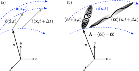
Figure 1: Kinematics of a material line element $\bm{\ell}$ and conformation tensor $\mathbf{A}=\left\langle\bm{\ell}\bm{\ell}\right\rangle$.

III The material derivative of a second-rank tensor

III.1 Conformation tensor

Consider an end-to-end vector $\bm{\mathbf{r}}$, whose magnitude at equilibrium is $r_{\rm eq}$. We define the dimensionless conformation tensor $\mathbf{A}\stackrel{{\scriptstyle\text{def}}}{{=}}\left\langle\bm{\mathbf{r}}\bm{\mathbf{r}}\right\rangle/r_{\rm eq}^{2}\stackrel{{\scriptstyle\text{def}}}{{=}}\left\langle\bm{\ell}\bm{\ell}\right\rangle$, where $\left\langle\cdot\right\rangle$ denotes the ensemble average and the dyadic product $\bm{\ell\ell}$ characterizes the state of deformation of a given microstructure, as sketched in Fig. 1(b); for example, $\mathbf{A}=\mathbf{I}$ represents an undeformed isotropic (equilibrium) state. For simplicity of the notation, we drop $\left\langle\cdot\right\rangle$ in the calculation that follows.

Proceeding formally to take the material derivative, and applying the product rule for differentiation, we obtain

$$\frac{D}{Dt}\mathbf{A}=\frac{D}{Dt}\left(\bm{\ell}\bm{\ell}\right)=\frac{D\bm{\ell}}{Dt}\bm{\ell}+\bm{\ell}\frac{D\bm{\ell}}{Dt}.$$ (9)

Using Eq. (2) and the properties of the dyadic product, we find

$$\frac{D}{Dt}\mathbf{A}=\frac{D}{Dt}\left(\bm{\ell}\bm{\ell}\right)=\bm{\ell}\cdot\left(\bm{\nabla}\mathbf{u}\right)\bm{\ell}+\bm{\ell}\bm{\ell}\cdot\left(\bm{\nabla}\mathbf{u}\right)=\left(\bm{\nabla}\mathbf{u}\right)^{T}\cdot\mathbf{A}+\mathbf{A}\cdot\bm{\nabla}\bm{u}.$$ (10)

This identity is also recognized in Ref. (Venerus and  Ottinger, 2018, Sec. 12.4). Therefore, we introduce a time derivative for the change of the tensor (dyadic product) deforming in a fluid flow:

$$\stackrel{{\scriptstyle\triangledown}}{{\mathbf{A}}}\stackrel{{\scriptstyle\text{def}}}{{=}}\frac{D}{Dt}\mathbf{A}-\left(\bm{\nabla}\mathbf{u}\right)^{T}\cdot\mathbf{A}-\mathbf{A}\cdot\bm{\nabla}\mathbf{u}.$$ (11)

The derivative $\stackrel{{\scriptstyle\triangledown}}{{\mathbf{A}}}$ is known as the upper-convected or contravariant time derivative Bird et al. (1987a). We conclude that $\stackrel{{\scriptstyle\triangledown}}{{\mathbf{A}}}={\bf 0}$ means that the conformation tensor deforms exactly as does the corresponding line elements in a flow. In contrast, $\stackrel{{\scriptstyle\triangledown}}{{\mathbf{A}}}\neq{\bf 0}$ means that $\mathbf{A}$ does not deform comparable to the line elements in the flow.

III.2 Arbitrary dyadic products and second-rank tensors

As a further remark, we note that the kinematic approach here is valid for any dyadic product. Since an arbitrary second-rank tensor, such as the stress tensor, can be written as a linear combination of three dyadic products (Brand, 1947, Secs. 61–63), then it follows that the derivation of the time derivatives discussed above also applies to an arbitrary second-rank tensor. For example, if we define the dyadic product ${\mathbf{B}}={\mathbf{a}}{\mathbf{b}}$, where $\mathbf{a}$ and $\mathbf{b}$ are vectors, then taking the material derivative and treating $\mathbf{a}$ and $\mathbf{b}$ as line elements (see Eq. (2)), we obtain

$$\frac{D}{Dt}\mathbf{B}=\frac{D}{Dt}\left(\mathbf{a}\mathbf{b}\right)=\frac{D\mathbf{a}}{Dt}\mathbf{b}+\mathbf{a}\frac{D\mathbf{b}}{Dt}=\mathbf{a}\cdot\left(\bm{\nabla}\mathbf{u}\right)\mathbf{b}+\mathbf{a}\mathbf{b}\cdot\left(\bm{\nabla}\mathbf{u}\right)=\left(\bm{\nabla}\mathbf{u}\right)^{T}\cdot\mathbf{B}+\mathbf{B}\cdot\bm{\nabla}\mathbf{u},$$ (12)

which is the form of the upper-convected derivative.

III.3 Invariance associated with convected time derivatives of the conformation tensor

Recall Sec. II on the kinematics of line elements, where the (Eulerian) time derivative $\stackrel{{\scriptstyle*}}{{\bm{\ell}}}=\bm{0}$ following the flow (Eq. (3)) implies the invariant solution $\bm{\mathbf{\ell}}_{L}\cdot\mathbf{F}^{-1}=\hbox{constant}$, from which the time variation of $\bm{\mathbf{\ell}}_{L}(t;\mathbf{X})$ can be determined for a given flow or $\mathbf{F}$ (see Eq. (8)). Following similar steps, one can take a Lagrangian view and integrate the equation $\stackrel{{\scriptstyle\triangledown}}{{\mathbf{A}}}=\frac{D\mathbf{A}}{Dt}-\left(\bm{\nabla}\mathbf{u}\right)^{T}\cdot\mathbf{A}-\mathbf{A}\cdot\bm{\nabla}\mathbf{u}=\bm{0}$. These ideas are known in the literature and the notation from Sec. II provides a compact way to proceed (see Supplementary Material). In particular, using a Lagrangian notation with $\mathbf{A}(\mathbf{x},t)=\mathbf{A}_{L}(t;\mathbf{X})$ one can show that $\stackrel{{\scriptstyle\triangledown}}{{\mathbf{A}}}=\bm{0}$ leads to

$$\frac{\partial}{\partial t}\left(\mathbf{F}^{-T}\cdot\mathbf{A}_{L}\cdot\mathbf{F}^{-1}\right)=\bm{0}.$$ (13)

It follows that $\mathbf{F}^{-T}\cdot\mathbf{A}_{L}\cdot\mathbf{F}^{-1}=\hbox{constant}$, following the fluid motion, i.e., it is an invariant. Using the initial data, we obtain $\mathbf{F}^{-T}\cdot\mathbf{A}_{L}\cdot\mathbf{F}^{-1}=\mathbf{A}_{L}(0;\mathbf{X})$ since $\mathbf{F}(0)=\mathbf{I}$, which means $\mathbf{A}_{L}(t;\mathbf{X})=\mathbf{F}^{T}\cdot\mathbf{A}_{L}(0;\mathbf{X})\cdot\mathbf{F}$. In other words, the initial data and $\mathbf{F}$ determine the evolution of the conformation tensor in this case.

IV The Jeffery equation for a particle in a linear flow

IV.1 A line element that lags the flow

A slender extensible filament or rod with orientation and length $\bm{\ell}$, not necessarily infinitesimal, in a flow with vorticity $\bm{\omega}=\bm{\nabla}\wedge\mathbf{u}$ and rate-of-strain tensor $\mathbf{E}=(1/2)(\bm{\nabla}\mathbf{u}+(\bm{\nabla}\mathbf{u})^{T})$ reorients approximately according to (see, e.g., Ericksen (1960); Gordon and E. (1971); Gordon and Schowalter (1972))

$$\frac{D\bm{\ell}}{Dt}=\frac{1}{2}\bm{\omega}\wedge\bm{\ell}+\beta\bm{\ell}\cdot\mathbf{E},$$ (14)

where $\beta$ is a constant. A rigid rod is unable to change length so Eq. (14) is then modified to preserve length by adding an extra term $-\beta\bm{\ell}\cdot\mathbf{E}\cdot\bm{\ell}\bm{\ell}$ to the right-hand side, resulting in the Jeffrey equation Jeffery (1922) (see Sec. V(vii)). Recalling the vorticity tensor $\bm{\Omega}=(1/2)(\bm{\nabla}\mathbf{u}-(\bm{\nabla}\mathbf{u})^{T})$, where $\bm{\nabla}\mathbf{u}=\mathbf{E}+\bm{\Omega}$ and $(1/2)\bm{\omega}\wedge\bm{\ell}=\bm{\ell}\cdot\bm{\Omega}$, Eq. (14) can be written as

$$\frac{D\bm{\ell}}{Dt}=\bm{\ell}\cdot\bm{\nabla}\mathbf{u}+\left(\beta-1\right)\bm{\ell}\cdot\mathbf{E},$$ (15)

where the last term indicates that the straining motion produces non-affine motion of the filament, relative to following the motion and deformation of the fluid. Therefore, a filament behaves like a line element and follows the flow for $\beta=1$, and lags the deformation for $\beta<1$, as arises below.

IV.2 A surface element

In the same way that the divergence of the velocity vector expresses the fractional rate of change of volume ($V)$ of an infinitesimal fluid element in a flow (so is zero for an incompressible flow), and a line element $\bm{\ell}$ changes it length and orientation according to Eq. (2), one can consider an infinitesimal (vectorial) surface element $\mathbf{S}$, i.e., $V=\bm{\ell}\cdot\mathbf{S}$. It is an exercise to show that for an incompressible flow, $\bm{\nabla}\cdot\mathbf{u}=0$, then (see, e.g., (Batchelor, 2000, pp. 131–132) and Stone (2017); Eggers et al. (2023))

$$\frac{D\mathbf{S}}{Dt}=-\left(\nabla\mathbf{u}\right)\cdot\mathbf{S}=\frac{1}{2}\bm{\omega}\wedge\mathbf{S}-\mathbf{S}\cdot\mathbf{E}.$$ (16)

Hence, we see that an infinitesimal surface element satisfies Eq. (14) with $\beta=-1$.

V Non-affine motion of the conformation tensor

The derivation of Eq. (11), and the steps that now follow, are the main contributions of this note focusing on the meaning of time derivatives for the kinematics of fluids with deformable microstructure. Substituting Eq. (15) into Eq. (9), we obtain

$$\frac{D}{Dt}\mathbf{A}=\frac{D}{Dt}\left(\bm{\ell}\bm{\ell}\right)=\left(\bm{\nabla}\mathbf{u}\right)^{T}\cdot\mathbf{A}+\mathbf{A}\cdot\bm{\nabla}\mathbf{u}+\left(\beta-1\right)\left(\mathbf{A}\cdot\mathbf{E}+\mathbf{E}\cdot\mathbf{A}\right),$$ (17)

or, using the definition of $\stackrel{{\scriptstyle\triangledown}}{{\mathbf{A}}}$,

$$\stackrel{{\scriptstyle\triangledown}}{{\mathbf{A}}}=\frac{D}{Dt}\mathbf{A}-\left(\bm{\nabla}\mathbf{u}\right)^{T}\cdot\mathbf{A}-\mathbf{A}\cdot\bm{\nabla}\mathbf{u}=\left(\beta-1\right)\left(\mathbf{A}\cdot\mathbf{E}+\mathbf{E}\cdot\mathbf{A}\right).$$ (18)

The right-hand side of Eq. (18) yields non-affine motion that changes the response from purely following the deformation of the fluid, i.e., we no longer have $\stackrel{{\scriptstyle\triangledown}}{{\mathbf{A}}}={\bf 0}$. We next make several observations.

1. $\beta=1$: We observe that $\beta=1$ gives back the case of a line element following the flow, i.e., the upper-convected derivative vanishes, i.e., $\stackrel{{\scriptstyle\triangledown}}{{\mathbf{A}}}={\bf 0}$.

2. $\beta=0$: Using the relation $\bm{\Omega}=\bm{\nabla}\mathbf{u}-\mathbf{E}$, we obtain

   $$\stackrel{{\scriptstyle\circ}}{{\mathbf{A}}}\stackrel{{\scriptstyle\text{def}}}{{=}}\frac{D}{Dt}\mathbf{A}-\bm{\Omega}^{T}\cdot\mathbf{A}-\mathbf{A}\cdot\bm{\Omega}=\bm{0}.$$ (19)

   $\stackrel{{\scriptstyle\circ}}{{\mathbf{A}}}$ is referred to as the (Jaumann) co-rotational derivative Zaremba (1903); Jaumann (1911), representing the rate of change of a fluid element advected with the flow and rotating with the local vorticity, e.g., see Eq. (14).

3. $\beta=-1$: In this case, using the definition for the rate-of-strain tensor $\mathbf{E}=(1/2)(\bm{\nabla}\mathbf{u}+(\bm{\nabla}\mathbf{u})^{T})$, Eq. (17) becomes

   $$\frac{D}{Dt}\mathbf{A}=\left(\bm{\nabla}\mathbf{u}\right)^{T}\cdot\mathbf{A}+\mathbf{A}\cdot\bm{\nabla}\mathbf{u}-2\left(\mathbf{A}\cdot\mathbf{E}+\mathbf{E}\cdot\mathbf{A}\right)=-\left(\bm{\nabla}\mathbf{u}\right)\cdot\mathbf{A}-\mathbf{A}\cdot\left(\bm{\nabla}\mathbf{u}\right)^{T}.$$ (20)

   Similar to Eq. (11), we can introduce the lower-convected or covariant time derivative (see, e.g., Bird et al. (1987a); Larson (1988); Hinch and Harlen (2021)):

   $$\overset{\vartriangle}{\mathbf{A}}\stackrel{{\scriptstyle\text{def}}}{{=}}\frac{D}{Dt}\mathbf{A}+\left(\bm{\nabla}\mathbf{u}\right)\cdot\mathbf{A}+\mathbf{A}\cdot\left(\bm{\nabla}\mathbf{u}\right)^{T}.$$ (21)

4. $\beta=\mathrm{const}$: For a constant value of $\beta$, using Eq. (17), we can introduce the Gordon$-$Schowalter convected time derivative $\overset{\square}{\mathbf{A}}$ (see, e.g., Gordon and Schowalter (1972); Larson (1988); Hinch and Harlen (2021)),

   $$\stackrel{{\scriptstyle\square}}{{\mathbf{A}}}\stackrel{{\scriptstyle\text{def}}}{{=}}\frac{D}{Dt}\mathbf{A}-\left(\bm{\nabla}\mathbf{u}\right)^{T}\cdot\mathbf{A}-\mathbf{A}\cdot\bm{\nabla}\mathbf{u}-\left(\beta-1\right)\left(\mathbf{A}\cdot\mathbf{E}+\mathbf{E}\cdot\mathbf{A}\right).$$ (22)

5. We note that, in practice, $\beta$, appearing in Eq. (22), can be a function of the conformation tensor $\mathbf{A}$. In fact, for a dumbbell model, Hinch (1977) and Phan-Thien et al. (1984) pointed out that $\beta$ depends on the trace of $\mathbf{A}$ via

   $$\beta=\frac{\mathrm{tr}\mathbf{A}-a}{\mathrm{tr}\mathbf{A}+b},$$ (23)

   where $\mathrm{tr}\mathbf{A}$ represents the square of the dumbbell extension and $a$ and $b$ are constants (see also Rallison and Hinch (1988); Hinch and Harlen (2021)).

6. An interesting property of the conformation tensor $\mathbf{A}$ that satisfies $\stackrel{{\scriptstyle\triangledown}}{{\mathbf{A}}}={\bf 0}$ (upper-convected derivative) is that its inverse $\mathbf{A}^{-1}$ satisfies $\left(\mathbf{A}^{-1}\right)^{\vartriangle}={\bf 0}$ (lower-convected derivative). This result can be readily shown by left and right multiplying $\stackrel{{\scriptstyle\triangledown}}{{\mathbf{A}}}={\bf 0}$ by $\mathbf{A}^{-1}$ and using the identity $\frac{\partial\mathbf{A}^{-1}}{\partial t}=-\mathbf{A}^{-1}\cdot\frac{\partial\mathbf{A}}{\partial t}\cdot\mathbf{A}^{-1}$. Similarly, $\stackrel{{\scriptstyle\circ}}{{\mathbf{A}}}={\bf 0}$ (co-rotational derivative) implies that $\left(\mathbf{A}^{-1}\right)^{\circ}={\bf 0}$. In fact, this symmetric property is more general and can be extended to the Gordon$-$Schowalter convected time derivative $\overset{\square}{\mathbf{A}}$, that if $\overset{\square}{\mathbf{A}}_{\beta}={\bf 0}$ for some $\beta$, then $\left(\mathbf{A}^{-1}\right)_{-\beta}^{\square}={\bf 0}$ with $-\beta$.

7. For a rigid inextensible rod, we modify Eq. (14) to preserve the length of the rod by including an additional term $-\beta\bm{\ell}\cdot\mathbf{E}\cdot\bm{\ell}\bm{\ell}$ on the right-hand side. Thus, we have the Jeffrey equation for the motion of a rigid ellipsoid Jeffery (1922),

   $$\frac{D\bm{\ell}}{Dt}=\frac{1}{2}\bm{\omega}\wedge\bm{\ell}+\beta\left(\bm{\ell}\cdot\mathbf{E}-\bm{\ell}\cdot\mathbf{E}\cdot\bm{\ell}\bm{\ell}\right),$$ (24)

   which also can be written as

   $$\frac{D\bm{\ell}}{Dt}=\bm{\ell}\cdot\bm{\nabla}\mathbf{u}+(\beta-1)\bm{\ell}\cdot\mathbf{E}-\beta\bm{\ell}\cdot\mathbf{E}\cdot\bm{\ell}\bm{\ell}.$$ (25)

   Here, the parameter $\beta$ is $\beta=(r^{2}-1)/(r^{2}+1)$, where $r$ is the length-to-radius aspect ratio of an axisymmetric ellipsoid Jeffery (1922). Substituting Eq. (24) into Eq. (9), we obtain the time-rate-of-change of the corresponding conformation tensor,

   $$\frac{D}{Dt}\mathbf{A}=\frac{D}{Dt}\left(\bm{\ell}\bm{\ell}\right)=\left(\bm{\nabla}\mathbf{u}\right)^{T}\cdot\mathbf{A}+\mathbf{A}\cdot\bm{\nabla}\mathbf{u}+(\beta-1)\left(\mathbf{A}\cdot\mathbf{E}+\mathbf{E}\cdot\mathbf{A}\right)-2\beta\mathbf{A}\cdot\mathbf{E}\cdot\mathbf{A}.$$ (26)

   Using the definition of $\stackrel{{\scriptstyle\triangledown}}{{\mathbf{A}}}$ yields,

   $$\stackrel{{\scriptstyle\triangledown}}{{\mathbf{A}}}=\frac{D}{Dt}\mathbf{A}-\left(\bm{\nabla}\mathbf{u}\right)^{T}\cdot\mathbf{A}-\mathbf{A}\cdot\bm{\nabla}\mathbf{u}=\left(\beta-1\right)\left(\mathbf{A}\cdot\mathbf{E}+\mathbf{E}\cdot\mathbf{A}\right)-2\beta\mathbf{A}\cdot\mathbf{E}\cdot\mathbf{A}.$$ (27)

   Again, we see how $\beta$ causes the conformation tensor to evolve differently than a “passive” structure simply following the fluid flow, $\stackrel{{\scriptstyle\triangledown}}{{\mathbf{A}}}\neq{\bf 0}$. As noted by Hinch and Harlen (2021), fibers, long thin rods, and elongated particles with $r\gg 1$ behave like line elements (of zero thickness) for which $\beta\approx 1$, so that the upper-convected derivative is appropriate. On the other hand, flattened particles with $r\ll 1$ behave like area elements, so that $\beta\approx-1$, and thus, the lower-convected derivative is appropriate.

8. As a particular case of the time derivative in Eq. (27), consider the case with $\beta=1$. We refer to this time derivative as the constrained upper-convected time derivative, given as

   $$\stackrel{{\scriptstyle\triangledown}}{{\mathbf{A}}}+2\mathbf{A}\cdot\mathbf{E}\cdot\mathbf{A}=\frac{D}{Dt}\mathbf{A}-\left(\bm{\nabla}\mathbf{u}\right)^{T}\cdot\mathbf{A}-\mathbf{A}\cdot\bm{\nabla}\mathbf{u}+2\mathbf{A}\cdot\mathbf{E}\cdot\mathbf{A}=\bm{0}.$$ (28)

   This time derivative arises, for example, in the so-called quadratic closure for the Doi-Onsager rod theory as shown in Weady et al. (2022) and in the sharply aligned case of the Doi-Onsager rod theory Gao et al. (2017). It is possible to extend the ideas introduced above (Sections II and III.3) for identifying invariances following the fluid motion to the special case of $\stackrel{{\scriptstyle\triangledown}}{{\mathbf{A}}}\neq{\bf 0}$ when $\stackrel{{\scriptstyle\triangledown}}{{\mathbf{A}}}=-2\mathbf{A}\cdot\mathbf{E}\cdot\mathbf{A}$.

   For example, using a Lagrangian notation with $\mathbf{A}(\mathbf{x},t)=\mathbf{A}_{L}(t;\mathbf{X})$ one can show (see Supplementary Material) that Eq. (28) leads to

   $$\frac{\partial}{\partial t}\left(\mathbf{F}^{-T}\cdot\mathbf{A}_{L}\cdot\mathbf{F}^{-1}\right)=-\left(\mathbf{F}^{-T}\cdot\mathbf{A}_{L}\cdot\mathbf{F}^{-1}\right)\cdot\frac{\partial}{\partial t}\left(\mathbf{F}\cdot\mathbf{F}^{T}\right)\cdot\left(\mathbf{F}^{-T}\cdot\mathbf{A}_{L}\cdot\mathbf{F}^{-1}\right).$$ (29)

   or

   $$\frac{\partial\mathbf{G}_{L}}{\partial t}=-\mathbf{G}_{L}\cdot\frac{\partial}{\partial t}\left(\mathbf{F}\cdot\mathbf{F}^{T}\right)\cdot\mathbf{G}_{L}\qquad\mathrm{with}\qquad\mathbf{G}_{L}=\mathbf{F}^{-T}\cdot\mathbf{A}_{L}\cdot\mathbf{F}^{-1}.$$ (30)

   Under the assumption that $\mathbf{G}_{L}$ (in fact, $\mathbf{A}_{L}$) is invertible and using the identities $\mathbf{G}_{L}^{-1}=\mathbf{F}\cdot\mathbf{A}_{L}^{-1}\cdot\mathbf{F}^{T}$ and $\frac{\partial\mathbf{G}_{L}}{\partial t}=-\mathbf{G}_{L}\cdot\frac{\partial\mathbf{G}_{L}^{-1}}{\partial t}\cdot\mathbf{G}_{L}$, from Eq. (30) it follows that

   $$\frac{\partial\mathbf{G}_{L}^{-1}}{\partial t}=\frac{\partial}{\partial t}\left(\mathbf{F}\cdot\mathbf{F}^{T}\right)\qquad\mathrm{or}\qquad\frac{\partial}{\partial t}\left(\mathbf{G}_{L}^{-1}-\mathbf{F}\cdot\mathbf{F}^{T}\right)=\frac{\partial}{\partial t}\left(\mathbf{F}\cdot\mathbf{A}_{L}^{-1}\cdot\mathbf{F}^{T}-\mathbf{F}\cdot\mathbf{F}^{T}\right)=\bm{0}.$$ (31)

   It follows that $\mathbf{F}\cdot\mathbf{A}_{L}^{-1}\cdot\mathbf{F}^{T}-\mathbf{F}\cdot\mathbf{F}^{T}=\hbox{constant}$, following the fluid motion, i.e., it is an invariant. Using the initial data, we obtain $\mathbf{F}\cdot\mathbf{A}_{L}^{-1}\cdot\mathbf{F}^{T}-\mathbf{F}\cdot\mathbf{F}^{T}=\mathbf{A}_{L}^{-1}(0;\mathbf{X})-\mathbf{I}$ since $\mathbf{F}(0)=\mathbf{I}$, which means $\mathbf{A}_{L}^{-1}(t;\mathbf{X})=\mathbf{I}-\mathbf{F}^{-1}\cdot\mathbf{F}^{-T}+\mathbf{F}^{-1}\cdot\mathbf{A}_{L}^{-1}(0;\mathbf{X})\cdot\mathbf{F}^{-T}$. Note that if $\mathbf{A}_{L}(0;\mathbf{X})=\mathbf{I}$, then $\mathbf{A}_{L}=\mathbf{I}$, which is a steady-state solution of Eq. (28).

   By analogy to Eq. (30) for the constrained upper-convected time derivative, one can show (see Supplementary Material) for the constrained lower-convected time derivative, $\overset{\vartriangle}{\mathbf{A}}=2\mathbf{A}\cdot\mathbf{E}\cdot\mathbf{A}$, that

   $$\frac{\partial}{\partial t}\left(\mathbf{H}_{L}^{-1}-\mathbf{F}^{-T}\cdot\mathbf{F}^{-1}\right)=\frac{\partial}{\partial t}\left(\mathbf{F}^{-T}\cdot\mathbf{A}_{L}^{-1}\cdot\mathbf{F}^{-1}-\mathbf{F}^{-T}\cdot\mathbf{F}^{-1}\right)=\bm{0}\qquad\mathrm{with}\qquad\mathbf{H}_{L}=\mathbf{F}\cdot\mathbf{A}_{L}\cdot\mathbf{F}^{T}.$$ (32)

   Thus, $\mathbf{F}^{-T}\cdot\mathbf{A}_{L}^{-1}\cdot\mathbf{F}^{-1}-\mathbf{F}^{-T}\cdot\mathbf{F}^{-1}$ is an invariant following the motion.

   For the constrained upper-/lower-convected derivatives, we have conserved quantities $\mathbf{G}_{L}=\mathbf{F}^{-T}\cdot\mathbf{A}_{L}\cdot\mathbf{F}^{-1}$ and $\mathbf{H}_{L}=\mathbf{F}\cdot\mathbf{A}_{L}\cdot\mathbf{F}^{T}$, respectively, whose invariant structure is essentially through inverses of each other. The co-rotational derivative arises from adding these two transport derivatives together, thus suggesting that finding an invariance for the co-rotational time derivative is challenging, if possible at all.

VI Connecting conformation and its change to stress

VI.1 The continuity and Cauchy momentum equations with additional microstructural stresses

Although the focus of this note is on the time derivatives, it is natural to now ask about the physical effects that exert forces on suspended filaments, which cause additional changes to these material derivatives and contribute to stress in the fluid. Describing the incompressible hydrodynamics of a complex fluid generally requires incorporating two new equations for the conformation tensor in addition to the continuity and Cauchy momentum equations. The first equation indicates how changes in the conformation give rise to stress in the fluid, whereas the second equation connects the evolution of the conformation to the gradients in the velocity field. As a specific example, consider the case of a viscoelastic dilute polymer solution, whose fluid motion is governed by the continuity equation and Cauchy momentum equations,

$$\bm{\nabla\cdot}\mathbf{u}=0\qquad\hbox{and}\qquad\rho\frac{D\mathbf{u}}{Dt}=\bm{\nabla\cdot}\bm{\sigma},$$ (33)

where $\rho$ is fluid density and $\bm{\sigma}$ is the stress tensor given by

$$\bm{\sigma}=-p\mathbf{I}+2\eta_{s}\mathbf{E}+\bm{\tau}_{p}.$$ (34)

The first term on the right-hand side of Eq. (34) is the pressure contribution, the second term is the viscous stress contribution of Newtonian solvent with a constant viscosity $\eta_{s}$, and the last term, $\bm{\tau}_{p}$, is the polymer contribution to the stress tensor. The latter contribution arises due to the response of polymer chains to fluid flow so that their microstructure deviates from the equilibrium state and deforms, $\mathbf{A}\neq\mathbf{I}$. This deformation results in a polymer contribution to the stress tensor, which, in the simplest Hookean case, can be expressed via $\mathbf{A}$ as (see, e.g., Snoeijer et al. (2020); Hinch and Harlen (2021); Beris (2021); Datta et al. (2022))

$$\bm{\tau}_{p}=G(\mathbf{A})(\mathbf{A}-\mathbf{I}),$$ (35)

where $G(\mathbf{A})$ is the elastic modulus, which may be a function of $\mathbf{A}$. Equations (33)$-$(35) show the coupling between the fluid velocity and deformation of microstructure. Understanding this two-way coupling also requires determining the evolution equation for the conformation changes that describes how polymer chains deform in the flow.

If we treat polymer chains like line elements transported and freely deformed by the flow, it implies $\stackrel{{\scriptstyle\triangledown}}{{\mathbf{A}}}={\bf 0}$, according to Eq. (11). However, polymer chains have elastic features with an inherent restoring mechanism opposing stretching/compression in the flow and causing relaxation to an equilibrium (coiled) state in the absence of flow. In general, this relaxation process may be characterized by several time scales; we denote by $\lambda$ the longest relaxation time of the polymers. Thus, for affine motion ($\beta=1$), accounting for the relaxation to an undeformed state on a time scale $\lambda$, the evolution equation for $\mathbf{A}$ can be written as

$$\stackrel{{\scriptstyle\triangledown}}{{\mathbf{A}}}=-\frac{1}{\lambda(\mathbf{A})}(\mathbf{A}-\mathbf{I}),$$ (36)

which, for a constant $\lambda$, is known as the Oldroyd-B constitutive equation Hinch and Harlen (2021); Beris (2021). We note that $\lambda(\mathbf{A})$ may be a function of $\mathbf{A}$, as was first elucidated by de Gennes (1974) and Hinch (1974).

From Eq. (36), it follows that when the observation time $t_{\rm obs}$ is much shorter than the relaxation time $\lambda$, $t_{\rm obs}\ll\lambda$, $\stackrel{{\scriptstyle\triangledown}}{{\mathbf{A}}}\approx{\bf 0}$ and thus, polymer chains behave like line elements that are transported and deformed by the flow without relaxing. We note that the ratio $\lambda/t_{\rm obs}$ is known as the Deborah number, $De\stackrel{{\scriptstyle\text{def}}}{{=}}\lambda/t_{\rm obs}$ Bird et al. (1987a, b), which follows from Eq. (36). In many cases, the observation time $t_{\rm obs}$ is based on the convective time scale $L_{c}/u_{c}$, where $L_{c}$ is the characteristic length scale and $u_{c}$ is the characteristic velocity, so that the Deborah number is $De=\lambda u_{c}/L_{c}$. Furthermore, as many flows are characterized by a shear rate, $\dot{\gamma}$, Eq. (36) also naturally introduces the Weissenberg number, $Wi=\lambda\dot{\gamma}$. While, for brevity, we have considered only the Oldroyd-B model, the approach illustrated here allows various physically plausible modifications similar to the modeling of dumbbells Hinch and Harlen (2021); Hinch (1974, 1977); de Gennes (1974); Bird et al. (1980); Fuller and Leal (1980, 1981); Phan-Thien et al. (1984); Dunlap and Leal (1987); Chilcott and Rallison (1988); Harrison et al. (1998); Remmelgas et al. (1999). Finally, we refer the reader to the recent work by Eggers et al. (2023) on flat elastic particles in a Newtonian fluid that, by analogy with dumbbell models, were modeled as three beads connected by nonlinear springs. In this work, a lower-convected time derivative naturally arises as part of the constitutive equation.

VI.2 Lagrangian integration of the Oldroyd-B constitutive equation

The ideas introduced above (Sections II and III.3) for identifying invariances following the fluid motion can also be applied to the evolution equation for the conformation tensor when elastic stresses are included. In this case, the conformation tensor evolves according to the deformation tensor $\mathbf{F}$ and the time constant $\lambda_{0}$. Again, the detailed steps can be found in the literature (see, e.g., (Bird et al., 1987a, pp. 431–432)), Hohenegger and Shelley (2011); Snoeijer et al. (2020) and Supplementary Material).

For example, we can consider the Oldroyd-B constitutive equation (Eq. (36)), $\stackrel{{\scriptstyle\triangledown}}{{\mathbf{A}}}=-\lambda_{0}^{-1}(\mathbf{A}-\mathbf{I})$, where $\lambda_{0}$ is a constant relaxation time. Again, we use the notation $\mathbf{A}(\mathbf{x},t)=\mathbf{A}_{L}(t;\mathbf{X})$. The equation for $\stackrel{{\scriptstyle\triangledown}}{{\mathbf{A}}}$ can be rearranged to find an ordinary differential equation for $\mathbf{F}^{-T}\cdot\mathbf{A}_{L}\cdot\mathbf{F}^{-1}$ with a time-dependent forcing,

$$\frac{\partial}{\partial t}\left(\mathbf{F}^{-T}\cdot\mathbf{A}_{L}\cdot\mathbf{F}^{-1}\right)+\frac{1}{\lambda_{0}}\mathbf{F}^{-T}\cdot\mathbf{A}_{L}\cdot\mathbf{F}^{-1}=\frac{1}{\lambda_{0}}\mathbf{F}^{-T}\cdot\mathbf{F}^{-1}.$$ (37)

This equation is solved with initial data (suppressing dependence on $\mathbf{X}$) $\mathbf{F}^{-T}\cdot\mathbf{A}_{L}\cdot\mathbf{F}^{-1}=\mathbf{A}_{L}(0)$ since $\mathbf{F}(0)=\mathbf{I}$. Therefore, integrating, we obtain (see also e.g. Hohenegger and Shelley (2011); Snoeijer et al. (2020)),

$$\mathbf{A}_{L}(t)=\hbox{e}^{-t/\lambda_{0}}\mathbf{F}^{T}(t)\cdot\mathbf{A}_{L}(0)\cdot\mathbf{F}(t)+\frac{1}{\lambda_{0}}\mathbf{F}^{T}(t)\cdot\int_{0}^{t}\mathbf{F}^{-T}\left(t^{\prime}\right)\cdot\mathbf{F}^{-1}\left(t^{\prime}\right)\hbox{e}^{-(t-t^{\prime})/\lambda_{0}}~{}{\rm d}t^{\prime}\cdot\mathbf{F}(t).$$ (38)

Thus, we observe that the flow history matters and the material is always relaxing, relative to the local flow features, according to an exponential in time. The reader is referred to Snoeijer et al. (2020) for more discussion and the connection of these ideas to the theory of elastic solids.

VII Concluding remarks

The approach illustrated here for the derivation of the typical time derivatives of the conformation tensor, Eqs. (11) and (18), commonly used in the study of the flow of complex fluids, is the main contribution of this note. Our derivation utilizes the idea of the kinematics of line elements, and we believe that the physical picture associated with this derivation may be useful in providing insight and developing intuition when using these time derivatives and the corresponding constitutive equations. For completeness, in Sec. VI, we briefly discussed the connection of the flow kinematics to the conformation changes that produce stresses. In several places in the discussion, we highlighted how a Lagrangian view of the kinematics allows one to identify invariances following the flow, or, in the case of elastic stresses, how the conformation tensor relaxes in a time-varying way relative to the stretch expected due to the flow alone.

Conflicts of interest

There are no conflicts to declare.

Supplementary Material for
A note about convected time derivatives for flows of complex fluids

S.1 Invariance associated with convected time derivatives of the conformation tensor

Recall Sec. II in the manuscript on the kinematics of line elements, where the (Eulerian) time derivative $\stackrel{{\scriptstyle*}}{{\bm{\ell}}}=\bm{0}$ following the flow ($\stackrel{{\scriptstyle*}}{{\bm{\ell}}}=\frac{D\bm{\ell}}{Dt}-\bm{\ell}\cdot\bm{\nabla}\mathbf{u}$) implies the invariant solution $\bm{\mathbf{\ell}}_{L}\cdot\mathbf{F}^{-1}=\hbox{constant}$, from which the time variation of $\bm{\mathbf{\ell}}_{L}(t;\mathbf{X})$ can be determined for a given flow or $\mathbf{F}$ (see Eq. (8)). Following similar steps, one can take a Lagrangian view and integrate the equation $\stackrel{{\scriptstyle\triangledown}}{{\mathbf{A}}}=\frac{D\mathbf{A}}{Dt}-\left(\bm{\nabla}\mathbf{u}\right)^{T}\cdot\mathbf{A}-\mathbf{A}\cdot\bm{\nabla}\mathbf{u}=\bm{0}$. We use the identities $\mathbf{F}^{-1}\cdot\mathbf{F}=\mathbf{I}$, $\mathbf{F}^{T}\cdot\mathbf{F}^{-T}=\mathbf{I}$, $\frac{\partial\mathbf{F}^{-T}}{\partial t}=-\mathbf{F}^{-T}\cdot\left(\bm{\nabla}\mathbf{u}\right)^{T}$, $\frac{\partial\mathbf{F}}{\partial t}=\mathbf{F}\cdot\bm{\nabla}\mathbf{u}$, and take a Lagrangian notation with $\mathbf{A}(\mathbf{x},t)=\mathbf{A}_{L}(t;\mathbf{X})$ to write

$$\stackrel{{\scriptstyle\triangledown}}{{\mathbf{A}}} = \frac{\partial\mathbf{A}_{L}}{\partial t}-\mathbf{F}^{T}\cdot\mathbf{F}^{-T}\cdot\left(\bm{\nabla}\mathbf{u}\right)^{T}\cdot\mathbf{A}_{L}-\mathbf{A}_{L}\cdot\mathbf{F}^{-1}\cdot\mathbf{F}\cdot\bm{\nabla}\mathbf{u}$$ (S1)

$$= \frac{\partial\mathbf{A}_{L}}{\partial t}+\mathbf{F}^{T}\cdot\frac{\partial\mathbf{F}^{-T}}{\partial t}\cdot\mathbf{A}_{L}-\mathbf{A}_{L}\cdot\mathbf{F}^{-1}\cdot\frac{\partial\mathbf{F}}{\partial t}=\frac{\partial\mathbf{A}_{L}}{\partial t}+\mathbf{F}^{T}\cdot\frac{\partial\mathbf{F}^{-T}}{\partial t}\cdot\mathbf{A}_{L}+\mathbf{A}_{L}\cdot\frac{\partial\mathbf{F}^{-1}}{\partial t}\cdot\mathbf{F}.$$

Right multiplying by $\mathbf{F}^{-1}$ and left multiplying by $\mathbf{F}^{-T}$ yields

$$\mathbf{F}^{-T}\cdot\stackrel{{\scriptstyle\triangledown}}{{\mathbf{A}}}\cdot\mathbf{F}^{-1}=\mathbf{F}^{-T}\cdot\frac{\partial\mathbf{A}_{L}}{\partial t}\cdot\mathbf{F}^{-1}+\frac{\partial\mathbf{F}^{-T}}{\partial t}\cdot\mathbf{A}_{L}\cdot\mathbf{F}^{-1}+\mathbf{F}^{-T}\cdot\mathbf{A}_{L}\cdot\frac{\partial\mathbf{F}^{-1}}{\partial t}=\frac{\partial}{\partial t}\left(\mathbf{F}^{-T}\cdot\mathbf{A}_{L}\cdot\mathbf{F}^{-1}\right).$$ (S2)

Thus, we conclude that $\stackrel{{\scriptstyle\triangledown}}{{\mathbf{A}}}=\bm{0}$ implies

$$\frac{\partial}{\partial t}\left(\mathbf{F}^{-T}\cdot\mathbf{A}_{L}\cdot\mathbf{F}^{-1}\right)=\bm{0}\quad\hbox{or}\quad\mathbf{F}^{-T}\cdot\mathbf{A}_{L}\cdot\mathbf{F}^{-1}=\hbox{constant},$$ (S3)

following the fluid motion, i.e., it is an invariant. Using the initial data, $\mathbf{F}^{-T}\cdot\mathbf{A}_{L}\cdot\mathbf{F}^{-1}=\mathbf{A}_{L}(0;\mathbf{X})$ since $\mathbf{F}(0)=\mathbf{I}$, which means $\mathbf{A}_{L}=\mathbf{F}^{T}\cdot\mathbf{A}_{L}(0;\mathbf{X})\cdot\mathbf{F}$. For example, if $\mathbf{A}_{L}(0;\mathbf{X})=\mathbf{I}$, i.e., an undeformed isotropic state, then $\mathbf{A}_{L}=\mathbf{F}^{T}\cdot\mathbf{F}$.

Similarly, one can show for the lower-convected time derivative that $\overset{\vartriangle}{\mathbf{A}}=\bm{0}$ implies $\frac{\partial}{\partial t}\left(\mathbf{F}\cdot\mathbf{A}_{L}\cdot\mathbf{F}^{T}\right)=\bm{0}$. Thus, $\mathbf{F}\cdot\mathbf{A}_{L}\cdot\mathbf{F}^{T}$ is an invariant following the motion.

S.2 Invariance associated with the constrained convected time derivative of the conformation tensor

It is possible to extend the ideas introduced above for identifying invariances following the fluid motion when $\stackrel{{\scriptstyle\triangledown}}{{\mathbf{A}}}=\bm{0}$ to the case of $\stackrel{{\scriptstyle\triangledown}}{{\mathbf{A}}}=-2\mathbf{A}\cdot\mathbf{E}\cdot\mathbf{A}$, corresponding to the constrained upper-convected time derivative.

Using a Lagrangian notation with $\mathbf{A}(\mathbf{x},t)=\mathbf{A}_{L}(t;\mathbf{X})$ and Eq. (S1), $\stackrel{{\scriptstyle\triangledown}}{{\mathbf{A}}}=-2\mathbf{A}\cdot\mathbf{E}\cdot\mathbf{A}$ can be expressed as

$$\stackrel{{\scriptstyle\triangledown}}{{\mathbf{A}}}=\frac{\partial\mathbf{A}_{L}}{\partial t}+\mathbf{F}^{T}\cdot\frac{\partial\mathbf{F}^{-T}}{\partial t}\cdot\mathbf{A}_{L}+\mathbf{A}_{L}\cdot\frac{\partial\mathbf{F}^{-1}}{\partial t}\cdot\mathbf{F}=-2\mathbf{A}_{L}\cdot\mathbf{E}\cdot\mathbf{A}_{L}.$$ (S4)

Right multiplying by $\mathbf{F}^{-1}$ and left multiplying by $\mathbf{F}^{-T}$ and using Eq. (S2), $\mathbf{F}^{-1}\cdot\mathbf{F}=\mathbf{I}$, and $\mathbf{F}^{T}\cdot\mathbf{F}^{-T}=\mathbf{I}$, Eq. (S4) yields

$$\frac{\partial}{\partial t}\left(\mathbf{F}^{-T}\cdot\mathbf{A}_{L}\cdot\mathbf{F}^{-1}\right)=-2\left(\mathbf{F}^{-T}\cdot\mathbf{A}_{L}\cdot\mathbf{F}^{-1}\right)\cdot\left(\mathbf{F}\cdot\mathbf{E}\cdot\mathbf{F}^{T}\right)\cdot\left(\mathbf{F}^{-T}\cdot\mathbf{A}_{L}\cdot\mathbf{F}^{-1}\right).$$ (S5)

Using the identities $\frac{\partial\mathbf{F}}{\partial t}=\mathbf{F}\cdot\bm{\nabla}\mathbf{u}$ and $\frac{\partial\mathbf{F}^{T}}{\partial t}=(\bm{\nabla}\mathbf{u})^{T}\cdot\mathbf{F}^{T}$, the term $2(\mathbf{F}\cdot\mathbf{E}\cdot\mathbf{F}^{T})$ in Eq. (S5) can be expressed as

$$2\left(\mathbf{F}\cdot\mathbf{E}\cdot\mathbf{F}^{T}\right)=\mathbf{F}\cdot\left(\bm{\nabla}\mathbf{u}+(\bm{\nabla}\mathbf{u})^{T}\right)\cdot\mathbf{F}^{T}=\frac{\partial\mathbf{F}}{\partial t}\cdot\mathbf{F}^{T}+\mathbf{F}\cdot\frac{\partial\mathbf{F}^{T}}{\partial t}=\frac{\partial}{\partial t}\left(\mathbf{F}\cdot\mathbf{F}^{T}\right),$$ (S6)

so that Eq. (S5) takes the form

$$\frac{\partial}{\partial t}\left(\mathbf{F}^{-T}\cdot\mathbf{A}_{L}\cdot\mathbf{F}^{-1}\right)=-\left(\mathbf{F}^{-T}\cdot\mathbf{A}_{L}\cdot\mathbf{F}^{-1}\right)\cdot\frac{\partial}{\partial t}\left(\mathbf{F}\cdot\mathbf{F}^{T}\right)\cdot\left(\mathbf{F}^{-T}\cdot\mathbf{A}_{L}\cdot\mathbf{F}^{-1}\right).$$ (S7)

or

$$\frac{\partial\mathbf{G}_{L}}{\partial t}=-\mathbf{G}_{L}\cdot\frac{\partial}{\partial t}\left(\mathbf{F}\cdot\mathbf{F}^{T}\right)\cdot\mathbf{G}_{L}\qquad\mathrm{with}\qquad\mathbf{G}_{L}=\mathbf{F}^{-T}\cdot\mathbf{A}_{L}\cdot\mathbf{F}^{-1}.$$ (S8)

Under the assumption that $\mathbf{G}_{L}$ (in fact, $\mathbf{A}_{L}$) is invertible and using the identities $\mathbf{G}_{L}^{-1}=\mathbf{F}\cdot\mathbf{A}_{L}^{-1}\cdot\mathbf{F}^{T}$ and $\frac{\partial\mathbf{G}_{L}}{\partial t}=-\mathbf{G}_{L}\cdot\frac{\partial\mathbf{G}_{L}^{-1}}{\partial t}\cdot\mathbf{G}_{L}$, from Eq. (S8) it follows that

$$\frac{\partial\mathbf{G}_{L}^{-1}}{\partial t}=\frac{\partial}{\partial t}\left(\mathbf{F}\cdot\mathbf{F}^{T}\right)\qquad\mathrm{or}\qquad\frac{\partial}{\partial t}\left(\mathbf{G}_{L}^{-1}-\mathbf{F}\cdot\mathbf{F}^{T}\right)=\frac{\partial}{\partial t}\left(\mathbf{F}\cdot\mathbf{A}_{L}^{-1}\cdot\mathbf{F}^{T}-\mathbf{F}\cdot\mathbf{F}^{T}\right)=\bm{0}.$$ (S9)

It follows that $\mathbf{F}\cdot\mathbf{A}_{L}^{-1}\cdot\mathbf{F}^{T}-\mathbf{F}\cdot\mathbf{F}^{T}=\hbox{constant}$, following the fluid motion, i.e., it is an invariant. Using the initial data, we obtain $\mathbf{F}\cdot\mathbf{A}_{L}^{-1}\cdot\mathbf{F}^{T}-\mathbf{F}\cdot\mathbf{F}^{T}=\mathbf{A}_{L}^{-1}(0;\mathbf{X})-\mathbf{I}$ since $\mathbf{F}(0)=\mathbf{I}$, which means $\mathbf{A}_{L}^{-1}(t;\mathbf{X})=\mathbf{I}-\mathbf{F}^{-1}\cdot\mathbf{F}^{-T}+\mathbf{F}^{-1}\cdot\mathbf{A}_{L}^{-1}(0;\mathbf{X})\cdot\mathbf{F}^{-T}$.

Similarly, one can show for the constrained lower-convected time derivative, $\overset{\vartriangle}{\mathbf{A}}=2\mathbf{A}\cdot\mathbf{E}\cdot\mathbf{A}$, that

$$\frac{\partial}{\partial t}\left(\mathbf{F}\cdot\mathbf{A}_{L}\cdot\mathbf{F}^{T}\right)=2\left(\mathbf{F}\cdot\mathbf{A}_{L}\cdot\mathbf{F}^{T}\right)\cdot\left(\mathbf{F}^{-T}\cdot\mathbf{E}\cdot\mathbf{F}^{-1}\right)\cdot\left(\mathbf{F}\cdot\mathbf{A}_{L}\cdot\mathbf{F}^{T}\right).$$ (S10)

Using the identities $\frac{\partial\mathbf{F}^{-T}}{\partial t}=-\mathbf{F}^{-T}\cdot\left(\bm{\nabla}\mathbf{u}\right)^{T}$ and $\frac{\partial\mathbf{F}^{-1}}{\partial t}=-\bm{\nabla}\mathbf{u}\cdot\mathbf{F}^{-1}$, the term $2(\mathbf{F}^{-T}\cdot\mathbf{E}\cdot\mathbf{F}^{-1})$ in Eq. (S10) can be expressed as

$$2\left(\mathbf{F}^{-T}\cdot\mathbf{E}\cdot\mathbf{F}^{-1}\right)=\mathbf{F}^{-T}\cdot\left(\bm{\nabla}\mathbf{u}+(\bm{\nabla}\mathbf{u})^{T}\right)\cdot\mathbf{F}^{-1}=-\mathbf{F}^{-T}\cdot\frac{\partial\mathbf{F}^{-1}}{\partial t}-\frac{\partial\mathbf{F}^{-T}}{\partial t}\cdot\mathbf{F}^{-1}=-\frac{\partial}{\partial t}\left(\mathbf{F}^{-T}\cdot\mathbf{F}^{-1}\right),$$ (S11)

so that Eq. (S10) takes the form

$$\frac{\partial}{\partial t}\left(\mathbf{F}\cdot\mathbf{A}_{L}\cdot\mathbf{F}^{T}\right)=-\left(\mathbf{F}\cdot\mathbf{A}_{L}\cdot\mathbf{F}^{T}\right)\cdot\frac{\partial}{\partial t}\left(\mathbf{F}^{-T}\cdot\mathbf{F}^{-1}\right)\cdot\left(\mathbf{F}\cdot\mathbf{A}_{L}\cdot\mathbf{F}^{T}\right),$$ (S12)

or

$$\frac{\partial\mathbf{H}_{L}}{\partial t}=-\mathbf{H}_{L}\cdot\frac{\partial}{\partial t}\left(\mathbf{F}^{-T}\cdot\mathbf{F}^{-1}\right)\cdot\mathbf{H}_{L}\qquad\mathrm{with}\qquad\mathbf{H}_{L}=\mathbf{F}\cdot\mathbf{A}_{L}\cdot\mathbf{F}^{T}.$$ (S13)

Again, under the assumption that $\mathbf{H}_{L}$ (in fact, $\mathbf{A}_{L}$) is invertible and using the identities $\mathbf{H}_{L}^{-1}=\mathbf{F}^{-T}\cdot\mathbf{A}_{L}^{-1}\cdot\mathbf{F}^{-1}$ and $\frac{\partial\mathbf{H}_{L}}{\partial t}=-\mathbf{H}_{L}\cdot\frac{\partial\mathbf{H}_{L}^{-1}}{\partial t}\cdot\mathbf{H}_{L}$, from Eq. (S13) it follows that

$$\frac{\partial\mathbf{H}_{L}^{-1}}{\partial t}=\frac{\partial}{\partial t}\left(\mathbf{F}^{-T}\cdot\mathbf{F}^{-1}\right)\qquad\mathrm{or}\qquad\frac{\partial}{\partial t}\left(\mathbf{H}_{L}^{-1}-\mathbf{F}^{-T}\cdot\mathbf{F}^{-1}\right)=\frac{\partial}{\partial t}\left(\mathbf{F}^{-T}\cdot\mathbf{A}_{L}^{-1}\cdot\mathbf{F}^{-1}-\mathbf{F}^{-T}\cdot\mathbf{F}^{-1}\right)=\bm{0}.$$ (S14)

Thus, $\mathbf{F}^{-T}\cdot\mathbf{A}_{L}^{-1}\cdot\mathbf{F}^{-1}-\mathbf{F}^{-T}\cdot\mathbf{F}^{-1}$ is an invariant following the motion.

S.3 Lagrangian integration of the Oldroyd-B constitutive equation

The ideas introduced in Sec. II and III C for identifying invariances following the fluid motion can also be applied to the evolution equation for the conformation tensor when elastic stresses are included. For example, consider the Oldroyd-B constitutive equation (Eq. (36)), $\stackrel{{\scriptstyle\triangledown}}{{\mathbf{A}}}=-\lambda_{0}^{-1}(\mathbf{A}-\mathbf{I})$, where $\lambda_{0}$ is a constant relaxation time. In this case, using Eq. (S1) and a Lagrangian notation with $\mathbf{A}(\mathbf{x},t)=\mathbf{A}_{L}(t;\mathbf{X})$, we have

$$\frac{\partial\mathbf{A}_{L}}{\partial t}+\mathbf{F}^{T}\cdot\frac{\partial\mathbf{F}^{-T}}{\partial t}\cdot\mathbf{A}_{L}+\mathbf{A}_{L}\cdot\frac{\partial\mathbf{F}^{-1}}{\partial t}\cdot\mathbf{F}=-\frac{1}{\lambda_{0}}(\mathbf{A}_{L}-\mathbf{I}).$$ (S15)

Now, recalling the steps just above, right multiplying by $\mathbf{F}^{-1}$ and left multiplying by $\mathbf{F}^{-T}$ yields

$$\frac{\partial}{\partial t}\left(\mathbf{F}^{-T}\cdot\mathbf{A}_{L}\cdot\mathbf{F}^{-1}\right)=-\frac{1}{\lambda_{0}}\mathbf{F}^{-T}\cdot(\mathbf{A}_{L}-\mathbf{I})\cdot\mathbf{F}^{-1}.$$ (S16)

Thus, we find an ordinary differential equation for $\mathbf{F}^{-T}\cdot\mathbf{A}_{L}\cdot\mathbf{F}^{-1}$ with a time-dependent forcing,

$$\frac{\partial}{\partial t}\left(\mathbf{F}^{-T}\cdot\mathbf{A}_{L}\cdot\mathbf{F}^{-1}\right)+\frac{1}{\lambda_{0}}\mathbf{F}^{-T}\cdot\mathbf{A}_{L}\cdot\mathbf{F}^{-1}=\frac{1}{\lambda_{0}}\mathbf{F}^{-T}\cdot\mathbf{F}^{-1}.$$ (S17)

This equation is to be solved with initial data (suppressing dependence on $\mathbf{X}$) $\mathbf{F}^{-T}\cdot\mathbf{A}_{L}\cdot\mathbf{F}^{-1}=\mathbf{A}_{L}(0)$ since $\mathbf{F}(0)=\mathbf{I}$. Therefore, integrating, we obtain (see, e.g. Hohenegger and Shelley (2011); Snoeijer et al. (2020)),

$$\mathbf{F}^{-T}(t)\cdot\mathbf{A}_{L}(t)\cdot\mathbf{F}^{-1}(t)=\hbox{e}^{-t/\lambda_{0}}\mathbf{A}_{L}(0)+\frac{1}{\lambda_{0}}\int_{0}^{t}\mathbf{F}^{-T}\left(t^{\prime}\right)\cdot\mathbf{F}^{-1}\left(t^{\prime}\right)\hbox{e}^{-(t-t^{\prime})/\lambda_{0}}~{}{\rm d}t^{\prime},$$ (S18)

or

$$\mathbf{A}_{L}(t)=\hbox{e}^{-t/\lambda_{0}}\mathbf{F}^{T}(t)\cdot\mathbf{A}_{L}(0)\cdot\mathbf{F}(t)+\frac{1}{\lambda_{0}}\mathbf{F}^{T}(t)\cdot\int_{0}^{t}\mathbf{F}^{-T}\left(t^{\prime}\right)\cdot\mathbf{F}^{-1}\left(t^{\prime}\right)\hbox{e}^{-(t-t^{\prime})/\lambda_{0}}~{}{\rm d}t^{\prime}\cdot\mathbf{F}(t).$$ (S19)

References

• Bird et al. (1987a) R. B. Bird, R. C. Armstrong, and O. Hassager, Dynamics of Polymeric Liquids. Volume 1: Fluid Mechanics, 2nd ed. (John Wiley and Sons, New York, 1987).
• Bird et al. (1987b) R. B. Bird, C. F. Curtiss, R. C. Armstrong, and O. Hassager, Dynamics of Polymeric Liquids. Volume 2: Kinetic theory, 2nd ed. (John Wiley and Sons, New York, 1987).
• Larson (1988) R. G. Larson, Constitutive Equations for Polymer Melts and Solutions (Butterworths, Boston, 1988).
• Oldroyd (1950) J. G. Oldroyd, On the formulation of rheological equations of state, Proc. R. Soc. A 200, 523 (1950).
• Kuhn (1934) W. Kuhn, Über die gestalt fadenförmiger moleküle in lösungen, Kolloid-Z. 68, 2 (1934).
• Morozov and Spagnolie (2015) A. Morozov and S. E. Spagnolie, Introduction to complex fluids, in Complex Fluids in Biological Systems, edited by S. E. Spagnolie (Springer, 2015) pp. 3–52.
• Lumley (1971) J. L. Lumley, Applicability of the Oldroyd constitutive equation to flow of dilute polymer solutions, Phys. Fluids 14, 2282 (1971).
• Hinch and Harlen (2021) J. Hinch and O. Harlen, Oldroyd B, and not A?, J. Non-Newtonian Fluid Mech. 298, 104668 (2021).
• Beris (2021) A. N. Beris, Continuum mechanics modeling of complex fluid systems following Oldroyd’s seminal 1950 work, J. Non-Newtonian Fluid Mech. 298, 104677 (2021).
• Datta et al. (2022) S. S. Datta, A. M. Ardekani, P. E. Arratia, A. N. Beris, I. Bischofberger, G. H. McKinley, J. G. Eggers, J. E. López-Aguilar, S. M. Fielding, A. Frishman, M. D. Graham, J. S. Guasto, S. J. Haward, A. Q. Shen, S. Hormozi, A. Morozov, R. J. Poole, V. Shankar, E. S. G. Shaqfeh, H. Stark, V. Steinberg, G. Subramanian, and H. A. Stone, Perspectives on viscoelastic flow instabilities and elastic turbulence, Phys. Rev. Fluids 7, 080701 (2022).
• Edwards and Beris (2023) B. J. Edwards and A. N. Beris, Oldroyd’s convected derivatives derived via the variational action principle and their corresponding stress tensors, J. Non-Newtonian Fluid Mech. 316, 105035 (2023).
• Hinch (1974) E. J. Hinch, Mechanical models of dilute polymer solutions for strong flows with large polymer deformations, Colloques Internationaux du CNRS 233, 241 (1974).
• Hinch (1977) E. J. Hinch, Mechanical models of dilute polymer solutions in strong flows, Phys. Fluids 20, S22 (1977).
• de Gennes (1974) P. G. de Gennes, Coil-stretch transition of dilute flexible polymers under ultrahigh velocity gradients, J. Chem. Phys. 60, 5030 (1974).
• Bird et al. (1980) R. B. Bird, P. J. Dotson, and N. L. Johnson, Polymer solution rheology based on a finitely extensible bead—spring chain model, J. Non-Newtonian Fluid Mech. 7, 213 (1980).
• Fuller and Leal (1980) G. G. Fuller and L. G. Leal, Flow birefringence of dilute polymer solutions in two-dimensional flows, Rheol. Acta 19, 580 (1980).
• Fuller and Leal (1981) G. G. Fuller and L. G. Leal, The effects of conformation-dependent friction and internal viscosity on the dynamics of the nonlinear dumbbell model for a dilute polymer solution, J. Non-Newtonian Fluid Mech. 8, 271 (1981).
• Phan-Thien et al. (1984) N. Phan-Thien, O. Manero, and L. G. Leal, A study of conformation-dependent friction in a dumbbell model for dilute solutions, Rheol. Acta 23, 151 (1984).
• Dunlap and Leal (1987) P. N. Dunlap and L. G. Leal, Dilute polystyrene solutions in extensional flows: Birefringence and flow modification, J. Non-Newtonian Fluid Mech. 23, 5 (1987).
• Chilcott and Rallison (1988) M. D. Chilcott and J. M. Rallison, Creeping flow of dilute polymer solutions past cylinders and spheres, J. Non-Newtonian Fluid Mech. 29, 381 (1988).
• Harrison et al. (1998) G. M. Harrison, J. Remmelgas, and L. G. Leal, The dynamics of ultradilute polymer solutions in transient flow: Comparison of dumbbell-based theory and experiment, J. Rheol. 42, 1039 (1998).
• Remmelgas et al. (1999) J. Remmelgas, P. Singh, and L. G. Leal, Computational studies of nonlinear elastic dumbbell models of Boger fluids in a cross-slot flow, J. Non-Newtonian Fluid Mech. 88, 31 (1999).
• Venerus and  Ottinger (2018) D. Venerus and H.  Ottinger, A Modern Course in Transport Phenomena (Cambridge University Press, Cambridge, 2018).
• Batchelor (2000) G. K. Batchelor, An Introduction to Fluid Dynamics (Cambridge University Press, 2000).
• Snoeijer et al. (2020) J. H. Snoeijer, A. Pandey, M. A. Herrada, and J. Eggers, The relationship between viscoelasticity and elasticity, Proc. R. Soc. Lond. A 476, 20200419 (2020).
• Brand (1947) L. Brand, Vector and Tensor Analysis (John Wiley & Sons, New York, 1947).
• Ericksen (1960) J. L. Ericksen, Transversely isotropic fluids, Kolloid Z. 173, 117 (1960).
• Gordon and E. (1971) R. J. Gordon and E. A. E., Bead-spring model of dilute polymer solutions: Continuum modifications and an explicit constitutive equation, J. Appl. Polym. Sci. 15, 1903 (1971).
• Gordon and Schowalter (1972) R. J. Gordon and W. R. Schowalter, Anisotropic fluid theory: a different approach to the dumbbell theory of dilute polymer solutions, Trans. Soc. Rheol. 16, 79 (1972).
• Jeffery (1922) G. B. Jeffery, The motion of ellipsoidal particles immersed in a viscous fluid, Proc. R. Soc. A 102, 161 (1922).
• Stone (2017) H. A. Stone, Fundamentals of fluid dynamics with an introduction to the importance of interfaces, in Soft Interfaces, Lecture Notes of the Les Houches Summer School, edited by L. Bocquet, D. Quéré, T. A. Witten, and L. F. Cugliandolo (Oxford University Press, New York, 2017) Chap. 1, pp. 3–76.
• Eggers et al. (2023) J. Eggers, T. B. Liverpool, and A. Mietke, Rheology of suspensions of flat elastic particles, preprint arXiv:2304.02980  (2023).
• Zaremba (1903) S. Zaremba, Remarques sur les travaux de M. Natanson relatifs à la théorie de la viscosité, Bull. Int. Acad. Sci. Crac. , 85 (1903).
• Jaumann (1911) G. Jaumann, Geschlossenes system physicalisher und chemischer differentialgesetze, Sitzber. Akad. Wiss. Wien (IIa) 120, 385 (1911).
• Rallison and Hinch (1988) J. M. Rallison and E. J. Hinch, Do we understand the physics in the constitutive equation?, J. Non-Newtonian Fluid Mech. 29, 37 (1988).
• Weady et al. (2022) S. Weady, D. B. Stein, and M. J. Shelley, Thermodynamically consistent coarse-graining of polar active fluids, Phys. Rev. Fluids 7, 063301 (2022).
• Gao et al. (2017) T. Gao, M. D. Betterton, A.-S. Jhang, and M. J. Shelley, Analytical structure, dynamics, and coarse graining of a kinetic model of an active fluid, Phys. Rev. Fluids 2, 093302 (2017).
• Hohenegger and Shelley (2011) C. Hohenegger and M. J. Shelley, Dynamics of Complex Bio-Fluids (Oxford University Press, Oxford, 2011).