A Nonsmooth Augmented Lagrangian Method and its Application to Poisson Denoising and Sparse Control

Abstract. In this paper, fully nonsmooth optimization problems in Banach spaces with finitely many inequality constraints, an equality constraint within a Hilbert space framework, and an additional abstract constraint are considered. First, we suggest a (safeguarded) augmented Lagrangian method for the numerical solution of such problems and provide a derivative-free global convergence theory which applies in situations where the appearing subproblems can be solved to approximate global minimality. Exemplary, the latter is possible in a fully convex setting. As we do not rely on any tool of generalized differentiation, the results are obtained under minimal continuity assumptions on the data functions. We then consider two prominent and difficult applications from image denoising and sparse optimal control where these findings can be applied in a beneficial way. These two applications are discussed and investigated in some detail. Due to the different nature of the two applications, their numerical solution by the (safeguarded) augmented Lagrangian approach requires problem-tailored techniques to compute approximate minima of the resulting subproblems. The corresponding methods are discussed, and numerical results visualize our theoretical findings.

Keywords. Augmented Lagrangian Method, Nonsmooth Optimization, Poisson Denoising, Semismooth Newton Method, Sparse Control

AMS subject classifications. 49M15, 49M37, 90C30, 90C48, 90C90

1 Introduction

Augmented Lagrangian methods provide a well-established framework for the numerical solution of constrained optimization problems, see e.g. [3, 5]. The method should be viewed as a general framework which allows an adaptation to many different scenarios simply by taking a suitable and problem-dependent subproblem solver. The two standard references mentioned above consider the situation of a general nonlinear program (in finite dimensions), but a suitable (global) convergence theory tailored for appropriate stationary points is also available for a couple of difficult, structured, and/or nonsmooth problems. This includes situations with an abstract geometric constraint (with potentially nonconvex constraint set), cf. [20, 27], programs with a composite objective function, see [12, 14, 15, 21, 31, 37]; specifically, [37] eliminates issues of nonsmoothness by exploiting smoothness properties of the Moreau envelope in a partially convex situation. The fully nonsmooth setting is also discussed in [17, 47], where all functions are smoothed, as well as in [33] in the framework of so-called difference-of-convex programs.

While these references mainly deal with finite-dimensional problems, the augmented Lagrangian approach can also be extended to the infinite-dimensional situation. Here, we distinguish between the “half” and “full” infinite-dimensional setting. Both settings share the property that the optimization variables belong to a Banach space, but the former allows only finitely many inequality constraints (possibly additional equality as well as abstract constraints), whereas the latter allows more general functional constraints living in a Banach space (say, $G(x)\in K$ for a mapping $G\colon X\to Y$ between two Banach spaces $X$ and $Y$ as well as a convex set $K\subset Y$). The convergence theory for the “half” infinite-dimensional setting was already considered in the seminal paper [36] by Rockafellar, see also the monograph [26]. Extensions to the fully infinite-dimensional setting are given in [8, 9, 29].

We should note, however, that there exist different versions for a realization of the augmented Lagrangian approach. In particular, there is the classical method with the standard Hestenes–Powell–Rockafellar update of the Lagrange multipliers, and there is the safeguarded version with a more careful updating of the multiplier estimates, see [5]. The counterexample in [28] shows that there cannot exist a satisfactory global convergence theory for the classical method, at least not in the nonconvex setting, while the existing convergence theory for the safeguarded version is rather complete in the sense that it has all desirable (and realistic) properties. On the other hand, for convex problems, there exists a convergence theory for the classical approach even with a constant penalty parameter. This result was established by Rockafellar [36], even for the “half” infinite-dimensional setting, and is based on the duality of the augmented Lagrangian and the proximal point method, see [37] as well. In particular, this convergence theory is based on the existence of optimal Lagrange multipliers.

In this paper, we also consider the “half” infinite-dimensional setting and investigate the convergence behavior of the safeguarded augmented Lagrangian method. The approach is fully motivated by the two classes of problems that play a central role within this paper, namely the variational Poisson denoising problem and an optimal control problem with a single (hard) sparsity constraint. Both problem classes are nonsmooth and convex, apart from that, however, they are of a completely different nature and therefore require problem-tailored methods for the solution of the resulting subproblems. This also shows the flexibility of the augmented Lagrangian approach since it allows to choose or create suitable techniques depending on the structure of these subproblems.

The first application, variational Poisson denoising, aims to minimize a (smoothness- or sparsity-promoting) function over a set of local similarity measures which, on the one hand, are induced by a Poisson process modeling the chosen discrete observation points of the image and, on the other hand, are evaluated on a huge number of sub-boxes of the underlying image while being inherently nonsmooth as the involved Kullback–Leibler-divergence is a convex function whose domain is not the full space. Within our algorithmic framework, all these constraints are augmented, and the associated subproblem is solved with the aid of a suitable stochastic gradient method.

In our second application, to obtain sparse controls, we suggest to use, as a hard constraint, a single sparsity constraint which bounds the control’s $L^{1}$-norm from above by a given constant. This idea is developed in the exemplary setting of the optimal control of Poisson’s equation. For the numerical solution of the problem, the nonsmooth sparsity constraint is augmented. It is demonstrated that the corresponding subproblems can be tackled by solving the associated (nonsmooth) system of optimality conditions with the aid of a (local) semismooth Newton method.

Though both applications are convex, the purely primal convergence theory for our safeguarded augmented Lagrangian method is discussed in a more general nonconvex setting. We assume, however, that we are able to find an approximate global minimum of the resulting subproblems. This is a realistic scenario in the convex setting, but might also be applicable in some other situations (e.g., think of disjunctive constraint systems composed of finitely many convex branches). We note that we do not apply the classical augmented Lagrangian approach with its nice convergence property for convex problems from [36] since, on the one hand, the convergence theory is written down in the more general nonconvex setting (recall from [28] that the classical augmented Lagrangian technique fails to have suitable convergence properties in this setting), and since the variational Poisson denoising application is at least unlikely to satisfy any constraint qualification (thus violating the assumptions of the convergence theory from [36]).

The paper is organized in the following way. We begin with some notation and preliminary statements in Section 2. The safeguarded augmented Lagrangian method is stated and analyzed in Section 3, where we consider nonsmooth problems with finitely many inequality constraints, a general operator equation (representing, e.g., a partial differential equation), as well as an abstract convex constraint set such that the associated augmented Lagrangian subproblems can be solved up to approximate global optimality. This requirement is particularly reasonable for convex problems. The application of this method to the variational Poisson denoising problem and the sparse control problem, which we view as the main contributions of this paper, are discussed in Sections 4 and 5, respectively. We conclude with some final remarks in Section 6.

2 Notation and Preliminaries

2.1 Basic Notation

Let $\mathbb{R}$ denote the set of real numbers. We make use of $\overline{\mathbb{R}}:=\mathbb{R}\cup\{\infty\}$. Throughout the paper, for a given finite set $D$, $\#D$ is used to denote the cardinality of $D$. Let $n\in\mathbb{N}$ be a positive integer. For vectors $x,y\in\mathbb{R}^{n}$, $\max(x,y)\in\mathbb{R}^{n}$ and $\left|x\right|\in\mathbb{R}^{n}$ denote the componentwise maximum of $x$ and $y$ and the componentwise absolute value of $x$, respectively. For any $p\in[1,\infty]$, the $\ell_{p}$-norm of $x\in\mathbb{R}^{n}$ will be denoted by $\left\|x\right\|_{p}$.

Whenever $X$ is a Banach space, its norm will be denoted by $\left\|\cdot\right\|_{X}\colon X\to[0,\infty)$ if not stated otherwise. Strong and weak convergence of a sequence $\{x^{k}\}\subset X$ to $x\in X$ are represented by $x^{k}\to x$ and $x^{k}\rightharpoonup x$, respectively. If $K\subset\mathbb{N}$ is a set of infinite cardinality, we make use of $x^{k}\to_{K}x$ ($x^{k}\rightharpoonup_{K}x$) in order to express that the subsequence $\{x^{k}\}_{k\in K}$ converges (converges weakly) to $x$ as $k$ tends to $\infty$ in $K$ (which we denote by $k\to_{K}\infty$ for brevity). The (topological) dual space of $X$ will be represented by $X^{*}$, and the associated dual pairing is then denoted by $\left\langle\cdot,\cdot\right\rangle_{X}\colon X^{*}\times X\to\mathbb{R}$. Let $Y$ be another Banach space. If $A\colon X\to Y$ is a continuous linear operator, its norm will be denoted by $\left\|A\right\|$ as the underlying spaces $X$ and $Y$ will be clear from the context. Let $\operatorname{id}_{X}\colon X\to X$ be the identity mapping of $X$. If $h\colon X\to Y$ is Fréchet differentiable at $x\in X$, $h^{\prime}(x)\colon X\to Y$ denotes the derivative of $h$ at $x$. Similarly, if $X_{1}$ and $X_{2}$ are Banach spaces such that $X=X_{1}\times X_{2}$, and if $h$ is Fréchet differentiable at $x:=(x_{1},x_{2})\in X$, $h^{\prime}_{x_{1}}(x)\colon X_{1}\to Y$ denotes the partial derivative with respect to (w.r.t.) $x_{1}$ of $h$ at $x$. The inner product in a Hilbert space $H$ will be represented by $(\cdot,\cdot)_{H}\colon H\times H\to\mathbb{R}$.

For an arbitrary function $\varphi\colon X\to\overline{\mathbb{R}}$ defined on a Banach space $X$, $\operatorname{dom}\varphi:=\{x\in X\,|\,\varphi(x)<\infty\}$ is referred to as the domain of $\varphi$. Whenever $\varphi$ is convex and $\bar{x}\in\operatorname{dom}\varphi$ is chosen arbitrarily, the set

$$\partial\varphi(\bar{x}):=\{\xi\in X^{*}\,|\,\varphi(x)\geq\varphi(\bar{x})+\left\langle\xi,x-\bar{x}\right\rangle_{X}\,\forall x\in\operatorname{dom}\varphi\}$$

is called the subdifferential (in the sense of convex analysis) of $\varphi$ at $\bar{x}$.

For an integer $d\in\mathbb{N}$, a bounded open set $\Omega\subset\mathbb{R}^{d}$, and $p\in[1,\infty)$, $L^{p}(\Omega)$ denotes the Lebesgue space of (equivalence classes of) measurable functions $u\colon\Omega\to\mathbb{R}$ such that $\Omega\ni\omega\mapsto\left|u(\omega)\right|^{p}\in\mathbb{R}$ is integrable, and is equipped with the standard norm which we denote by $\left\|\cdot\right\|_{p}\colon L^{p}(\Omega)\to[0,\infty)$. Note that it will be clear from the context where $\left\|\cdot\right\|_{p}$ is taken in $\mathbb{R}^{n}$ or $L^{p}(\Omega)$. If $u\in L^{p}(\Omega)$ is arbitrary, we use the notation $\{u=0\}:=\{\omega\in\Omega\,|\,u(\omega)=0\}$ for brevity. The sets $\{u<0\}$ and $\{u>0\}$ are defined similarly. Note that $\{u=0\}$, $\{u<0\}$, and $\{u>0\}$ are well defined up to subsets of $\Omega$ possessing measure $0$. Whenever $\Omega^{\prime}\subset\Omega$ is measurable, $\chi_{\Omega^{\prime}}\colon\Omega\to\mathbb{R}$ denotes the characteristic function of $\Omega^{\prime}$ which is $1$ for arguments in $\Omega^{\prime}$ and, otherwise, $0$. Additionally, for any $u\in L^{p}(\Omega)$, we make use of the associated function $\operatorname{sign}(u)\colon\Omega\to\mathbb{R}$ which is given by $\operatorname{sign}(u):=\chi_{\{u>0\}}-\chi_{\{u<0\}}$. Finally, $H^{1}_{0}(\Omega)$ denotes the closure of $C^{\infty}_{c}(\Omega)$, the set of all arbitrarily often continuously differentiable functions with compact support in $\Omega$, w.r.t. the standard $H^{1}$-Sobolev norm. Throughout the paper, $H^{-1}(\Omega):=H^{1}_{0}(\Omega)^{*}$ is used.

2.2 Preliminary Results

In the following lemma, we study conditions which guarantee that the composition of a (weakly sequentially) lower semicontinuous function and a continuous function is (weakly sequentially) lower semicontinuous again.

Lemma 2.1.

For some Banach space $X$, let $\varphi\colon X\to\overline{\mathbb{R}}$ be weakly sequentially lower semicontinuous and let $\psi\colon\mathbb{R}\to\mathbb{R}$ be a continuous and monotonically increasing function. Then $\psi\circ\varphi\colon X\to\overline{\mathbb{R}}$ defined via

$$\forall x\in X\colon\quad(\psi\circ\varphi)(x):=\begin{cases}\psi(\varphi(x))&\text{if }\varphi(x)<\infty,\\ \lim_{t\to\infty}\psi(t)&\text{if }\varphi(x)=\infty\end{cases}$$

is weakly sequentially lower semicontinuous.

Proof: Choose $\{x^{k}\}\subset X$ and $\bar{x}\in X$ with $x^{k}\rightharpoonup\bar{x}$ arbitrarily and pick an infinite set $K\subset\mathbb{N}$ as well as a number $\alpha\in\overline{\mathbb{R}}$ such that

$$\alpha=\liminf_{k\to\infty}(\psi\circ\varphi)(x^{k})=\lim_{k\to_{K}\infty}(\psi\circ\varphi)(x^{k}).$$

In case $\alpha=\infty$, we automatically have $\alpha\geq(\psi\circ\varphi)(\bar{x})$ and, thus, there is nothing to show. Thus, we assume $\alpha\in\mathbb{R}$. By weak sequential lower semicontinuity of $\varphi$, we have $\beta:=\liminf_{k\to_{K}\infty}\varphi(x^{k})\geq\varphi(\bar{x})$. Pick an infinite set $K^{\prime}\subset K$ such that $\lim_{k\to_{K^{\prime}}\infty}\varphi(x^{k})=\beta$. In case where $\beta\in\mathbb{R}$ holds, $\varphi(\bar{x})$ and the tail of the sequence $\{\varphi(x^{k})\}_{k\in K^{\prime}}$ are finite, so we find

$$\alpha=\lim\limits_{k\to_{K^{\prime}}\infty}(\psi\circ\varphi)(x^{k})=\lim\limits_{k\to_{K^{\prime}}\infty}\psi(\varphi(x^{k}))=\psi(\beta)\geq\psi(\varphi(\bar{x}))=(\psi\circ\varphi)(\bar{x})$$

by continuity and monotonicity of $\psi$. Next, suppose that $\beta=\infty$ holds. In case where $\{\varphi(x^{k})\}_{k\in K^{\prime}}$ equals $\infty$ along the tail of the sequence, we find

$$\alpha=\lim\limits_{k\to_{K^{\prime}}\infty}(\psi\circ\varphi)(x^{k})=\lim\limits_{t\to\infty}\psi(t)\geq(\psi\circ\varphi)(\bar{x})$$

by monotonicity of $\psi$. Otherwise, there is an infinite set $K^{\prime\prime}\subset K^{\prime}$ such that $\{\varphi(x^{k})\}_{k\in K^{\prime\prime}}\subset\mathbb{R}$. However, $\beta=\infty$ yields $\lim_{k\to_{K^{\prime\prime}}\infty}\varphi(x^{k})=\infty$. Hence, by definition of the composition, we find

$$\alpha=\lim\limits_{k\to_{K^{\prime\prime}}\infty}(\psi\circ\varphi)(x^{k})=\lim\limits_{k\to_{K^{\prime\prime}}\infty}\psi(\varphi(x^{k}))=\lim\limits_{t\to\infty}\psi(t)\geq(\psi\circ\varphi)(\bar{x})$$

by continuity and monotonicity of $\psi$. This completes the proof. $\Box$

We would like to note that, in general, for a (weakly sequentially) lower semicontinuous function $\varphi\colon X\to\overline{\mathbb{R}}$, the mappings $x\mapsto|\varphi(x)|$ and $x\mapsto\varphi^{2}(x)$ are not (weakly sequentially) lower semicontinuous (exemplary, choose $X:=\mathbb{R}$ and set $\varphi(x):=-1$ for all $x\leq 0$ and $\varphi(x):=0$ for all $x>0$). Observe that the absolute value function and the square are not monotonically increasing, i.e., the assumptions of Lemma 2.1 are not satisfied in this situation.

We comment on a typical setting where Lemma 2.1 applies.

Example 2.2.

For each $\alpha>0$ and $\beta\in\mathbb{R}$, the function $\psi\colon\mathbb{R}\to\mathbb{R}$ given by $\psi(t):={\max}^{2}(0,\alpha t+\beta)$ for each $t\in\mathbb{R}$ is continuous, monotonically increasing, and satisfies $\lim_{t\to\infty}\psi(t)=\infty$. Thus, for each weakly sequentially lower semicontinuous function $\varphi\colon X\to\overline{\mathbb{R}}$, the composition $\psi\circ\varphi\colon X\to\overline{\mathbb{R}}$ given by

$$\forall x\in X\colon\quad(\psi\circ\varphi)(x):=\begin{cases}\psi(\varphi(x))&\text{if }\varphi(x)<\infty,\\ \infty&\text{if }\varphi(x)=\infty\end{cases}$$

is weakly sequentially lower semicontinuous as well by Lemma 2.1.

We also note that this particular function $\psi$ is convex. Thus, keeping the monotonicity of $\psi$ in mind, whenever $\varphi$ is convex, then the composition $\psi\circ\varphi$ is convex as well.

3 An Augmented Lagrangian Method for Nonsmooth Optimization Problems

In this section, we address the algorithmic treatment of the optimization problem

$$\min\ f(x)\quad\text{s.t.}\quad g(x)\leq 0,\ h(x)=0,\ x\in C,$$ (P)

where $f\colon X\to\overline{\mathbb{R}}$, $g\colon X\to\overline{\mathbb{R}}^{m}$, and $h\colon X\to Y$ are given functions and $C\subset X$ is a weakly sequentially closed set. Moreover, $X$ is a reflexive Banach space and $Y$ is a Hilbert space, which we identify with its dual, i.e., $Y\cong Y^{*}$. Throughout this section, we assume that the feasible set $\mathcal{F}\subset X$ of P satisfies $\mathcal{F}\cap\operatorname{dom}f\neq\emptyset$ in order to exclude trivial situations. For later use, we introduce $\operatorname{dom}g:=\bigcap_{i=1}^{m}\operatorname{dom}g_{i}$ and note that $\operatorname{dom}g\neq\emptyset$ since $\mathcal{F}\neq\emptyset$. Here, $g_{1},\ldots,g_{m}$ are the component functions of $g$.

In contrast to the standard setting of nonlinear programming, we abstain from demanding any differentiability properties of the data functions. However, we assume that the functions $f,g_{1},\ldots,g_{m}\colon X\to\overline{\mathbb{R}}$ are weakly sequentially lower semicontinuous, while the function $h$ is weakly-strongly sequentially continuous in the sense that

$$\forall\{x^{k}\}\subset X\colon\quad x^{k}\rightharpoonup\bar{x}\quad\text{in}\;X\quad\Longrightarrow\quad h(x^{k})\to h(\bar{x})\quad\text{in}\;Y.$$

Note that at least continuity of the function $h$ is indispensable in order to guarantee that $\mathcal{F}$ is closed. The assumptions from above already guarantee that $\mathcal{F}$ is weakly sequentially closed. Together with the weak sequential lower semicontinuity of the objective functional $f$, this can be interpreted as a minimal requirement in constrained optimization in order to ensure that the underlying optimization problem P possesses a solution. This would be inherent whenever $\mathcal{F}$ is, additionally, bounded or $f$ is, additionally, coercive as standard arguments show.

3.1 Statement of the Algorithm

For the construction of our solution method, we make use of the classical augmented Lagrangian function $L_{\rho}\colon X\times\mathbb{R}^{m}\times Y\to\overline{\mathbb{R}}$ associated with P which is given by

$$L_{\rho}(x,\lambda,\mu):=f(x) +\frac{1}{2\rho}\sum_{i=1}^{m}\left({\max}^{2}\left(0,\lambda_{i}+\rho g_{i}(x)\right)-\lambda_{i}^{2}\right)$$ (3.1)

$$+(\mu,h(x))_{Y}+\frac{\rho}{2}\left\|h(x)\right\|^{2}_{Y}$$

for all $x\in X$, $\lambda\in\mathbb{R}^{m}$, and $\mu\in Y$, where $\rho>0$ is a given penalty parameter. Within our algorithmic framework, the function $L_{\rho}$ has to be minimized w.r.t. $x$, which means that the term $-\tfrac{1}{2\rho}\left\|\lambda\right\|^{2}_{2}$ could be removed from the definition of $L_{\rho}$. However, for some of the proofs we are going to provide, it will be beneficial to keep this shift. We would like to point the reader’s attention to the fact that the function $L_{\rho}(\cdot,\lambda,\mu)$ is weakly sequentially lower semicontinuous for each $\lambda\in\mathbb{R}^{m}$ and $\mu\in Y$ due to Lemma 2.1, Example 2.2, and the fact that the function $h$ is weakly-strongly sequentially continuous.

Remark 3.1.

Whenever P is a convex optimization problem, i.e., whenever the functions $f,g_{1},\ldots,g_{m}$ are convex while $h$ is affine, then, for each $\lambda\in\mathbb{R}^{m}$ and $\mu\in Y$, $L_{\rho}(\cdot,\lambda,\mu)$ is a convex function as well by monotonicity and convexity of $t\mapsto{\max}^{2}(0,\alpha t+\beta)$ for each $\alpha>0$ and $\beta\in\mathbb{R}$.

For some penalty parameter $\rho>0$, we introduce a function $V_{\rho}\colon X\times\mathbb{R}^{m}\to\overline{\mathbb{R}}$ by means of

$$V_{\rho}(x,\lambda):=\begin{cases}\max\bigl{(}\left\|\max(g(x),-\lambda/\rho)\right\|_{\infty},\left\|h(x)\right\|_{Y}\bigr{)}&\text{if }x\in\operatorname{dom}g,\\ \infty&\text{if }x\notin\operatorname{dom}g\end{cases}$$

for all $x\in X$ and $\lambda\in\mathbb{R}^{m}$. Right from the definition of $V_{\rho}$, we obtain

$$V_{\rho}(x,\lambda)=0\quad\Longleftrightarrow\quad g(x)\leq 0,\,\lambda\geq 0,\,\lambda^{\top}g(x)=0,\,h(x)=0,$$

i.e., $V_{\rho}$ can be used to measure feasibility of $x$ for P w.r.t. the constraints induced by $g$ and $h$ as well as validity of the complementarity-slackness condition w.r.t. the inequality constraints.

In Algorithm 3.2, we state a pseudo-code which describes our method.

Algorithm 3.2 (Safeguarded Augmented Lagrangian Method for P).

1:bounded sets $B_{m}\subset\mathbb{R}^{m}$ and $B_{Y}\subset Y$, starting point $(x^{0},\lambda^{0},\mu^{0})\in C\times\mathbb{R}^{m}_{+}\times Y$, initial penalty parameter $\rho_{0}>0$, parameters $\tau\in(0,1)$, $\gamma>1$

2: Set $k:=0$.

3:while a suitable termination criterion is violated at iteration $k$ do

4:      Choose $v^{k}\in B_{m}$ and $w^{k}\in B_{Y}$.

5:      Compute $x^{k+1}\in C$ as an approximate solution of the optimization problem $$\min_{x}L_{\rho_{k}}(x,v^{k},w^{k})\quad\text{s.t.}\quad x\in C.$$ (3.2)

6:      Set $$\lambda^{k+1}:=\max\bigl{(}0,v^{k}+\rho_{k}g(x^{k+1})\bigr{)},\qquad\mu^{k+1}:=w^{k}+\rho_{k}h(x^{k+1}).$$ (3.3)

7:      If either $k=0$ or the condition $$V_{\rho_{k}}(x^{k+1},v^{k})\leq\tau\,V_{\rho_{k-1}}(x^{k},v^{k-1})$$ (3.4) holds, set $\rho_{k+1}:=\rho_{k}$, otherwise set $\rho_{k+1}:=\gamma\rho_{k}$.

8:      Set $k\leftarrow k+1$.

9:end while

10:return $x^{k}$

In Algorithm 3.2, the quantities $v^{k}$ and $w^{k}$ play the role of Lagrange multiplier estimates. By construction, the sequences $\{v^{k}\}$ and $\{w^{k}\}$ remain bounded throughout a run of the algorithm while this does not necessarily hold true for $\{\lambda^{k}\}$ and $\{\mu^{k}\}$. Note that the classical augmented Lagrangian method could be recovered from Algorithm 3.2 by replacing $v^{k}$ and $w^{k}$ by $\lambda^{k}$ and $\mu^{k}$ everywhere, respectively. However, the so-called safeguarded variant from Algorithm 3.2 has been shown to possess better global convergence properties than the classical method, see, e.g., [28] for details. Typically, $\{v^{k}\}$ and $\{w^{k}\}$ are iteratively constructed during the run of Algorithm 3.2. Exemplary, one can choose $B_{m}$ as the (very large) box $[0,\mathbf{v}]$ for some $\mathbf{v}\in\mathbb{R}^{m}$ satisfying $\mathbf{v}>0$ and define $v^{k}$ as the projection of $\lambda^{k}$ onto this box in 4. Note that this choice already incorporates desirable information about the sign of the correct Lagrange multipliers (in case of existence). A similar procedure is possible for the choice of $w^{k}$. This way, Algorithm 3.2 is likely to parallel the classical augmented Lagrangian method if the sequences $\{\lambda^{k}\}$ and $\{\mu^{k}\}$ remain bounded.

Assuming for a moment that all involved data functions are smooth, the derivative w.r.t. $x$ of $L_{\rho}$ from 3.1 is given by

$$(L_{\rho})^{\prime}_{x}(x,\lambda,\mu)=f^{\prime}(x)+\sum\limits_{i=1}^{m}\max(0,\lambda_{i}+\rho\,g_{i}(x))\,g^{\prime}_{i}(x)+h^{\prime}(x)^{*}[\mu+\rho h(x)].$$

Thus, the updating rule for the multipliers in 3.3 yields

$$(L_{\rho_{k}})^{\prime}_{x}(x^{k+1},v^{k},w^{k})=L^{\prime}_{x}(x^{k+1},\lambda^{k+1},\mu^{k+1}),$$ (3.5)

which is the basic idea behind 6. Here, $L\colon X\times\mathbb{R}^{m}\times Y\to{\overline{\mathbb{R}}}$ denotes the standard Lagrangian function associated with P which is given by

$$L(x,\lambda,\mu):=f(x)+\lambda^{\top}g(x)+(\mu,h(x))_{Y}$$

for $x\in X$, $\lambda\in\mathbb{R}^{m}$, and $\mu\in Y$. Note that a similar formula as 3.5 can be obtained in terms of several well-known concepts of subdifferentiation whenever a suitable chain rule applies.

Finally, let us mention that in 7, the penalty parameter is increased whenever the new iterate $(x^{k+1},v^{k},w^{k})$ is not (sufficiently) better from the viewpoint of feasibility (and complementarity) than the old iterate $(x^{k},v^{k-1},w^{k-1})$. Note that our choice for the infinity norm in the definition of $V_{\rho}$ is a matter of taste since all norms are equivalent in finite-dimensional spaces. However, this particular measure $V_{\rho}$ keeps track of the largest violation of the feasibility and complementarity condition w.r.t. all inequality constraints, which is why we favor it here.

For further information about (safeguarded) augmented Lagrangian methods in nonlinear programming, we refer the interested reader to [5].

3.2 Convergence to Global Minimizers

In this subsection, we provide a convergence analysis for Algorithm 3.2 where we assume that in 5, the subproblem 3.2 is solved to (approximate) global optimality. Exemplary, this is possible whenever P is a convex program, see Remark 3.1, but also in more general situations where P is of special structure, e.g. if the feasible set can be decomposed into a moderate number of convex branches while the objective function is convex. Within the assumption below, which will be standing throughout this section, we quantify the requirements regarding the subproblem solver.

Assumption 3.3.

In each iteration $k\in\mathbb{N}$ of Algorithm 3.2, the approximate solution $x^{k+1}\in C$ of 3.2 satisfies

$$L_{\rho_{k}}(x^{k+1},v^{k},w^{k})-\varepsilon_{k}\leq L_{\rho_{k}}(x,v^{k},w^{k})\qquad\forall x\in C$$ (3.6)

where $\varepsilon_{k}\geq 0$ is some given constant.

Typically, the inexactness parameter $\varepsilon_{k}$ in 3.3 is chosen to be positive. While $\varepsilon_{k}:=0$ corresponds to the situation where the subproblems 3.2 are solved exactly, we will see that the augmented Lagrangian technique generally works fine if only approximate solutions of the subproblems are computed. This also has the advantage that whenever $\inf_{x}\{L_{\rho_{k}}(x,v^{k},w^{k})\,|\,x\in C\}$ is finite, then one can always find points $x^{k+1}$ satisfying 3.6 for arbitrarily small $\varepsilon_{k}>0$ while an exact global minimizer may not exist. Furthermore, we note that, due to $\mathcal{F}\cap\operatorname{dom}f\neq\emptyset$, $L_{\rho_{k}}(x^{k+1},v^{k},w^{k})<\infty$ holds for each $k\in\mathbb{N}$, i.e., $x^{k+1}\in\operatorname{dom}f\cap\operatorname{dom}g\cap C$ holds for each computed iterate. Finally, it is worth mentioning that validity of 3.6 guarantees that $L_{\rho_{k}}(\cdot,v^{k},w^{k})$ is bounded from below on $C$.

Throughout the section, we make use of the following lemma.

Lemma 3.4.

Let $v\in\mathbb{R}^{m}$, $w\in Y$, and $\rho>0$ as well as a feasible point $x\in\mathcal{F}$ of P be arbitrary. Then $L_{\rho}(x,v,w)\leq f(x)$ is valid.

Proof: Due to $h(x)=0$ and by definition of the augmented Lagrangian function $L_{\rho}$ from 3.1, we find

$$L_{\rho}(x,v,w)=f(x)+\frac{1}{2\rho}\sum\limits_{i=1}^{m}\left({\max}^{2}(0,v_{i}+\rho\,g_{i}(x))-v_{i}^{2}\right),$$

i.e., in order to show the claim, it is sufficient to verify ${\max}^{2}(0,v_{i}+\rho\,g_{i}(x))\leq v_{i}^{2}$ for all $i\in\{1,\ldots,m\}$. Thus, fix $i\in\{1,\ldots,m\}$ arbitrarily. In case $v_{i}+\rho\,g_{i}(x)\leq 0$, we find ${\max}^{2}(0,v_{i}+\rho\,g_{i}(x))=0\leq v_{i}^{2}$. Conversely, $v_{i}+\rho\,g_{i}(x)>0$ yields $0\leq v_{i}+\rho\,g_{i}(x)\leq v_{i}$ since $g_{i}(x)\leq 0$ is valid by feasibility of $x$ for P, so by monotonicity of the square on the non-negative real line, ${\max}^{2}(0,v_{i}+\rho\,g_{i}(x))\leq v_{i}^{2}$ follows. $\Box$

Let us now start with the convergence analysis associated with Algorithm 3.2. Therefore, we first study issues related to the feasibility of limit points.

Proposition 3.5.

Assume that Algorithm 3.2 produces a sequence $\{x^{k}\}$ such that 3.3 holds for some bounded sequence $\{\varepsilon_{k}\}$, and let $\{\rho_{k}\}$ and $\{v^{k}\}$ be the associated sequences of penalty parameters and Lagrange multiplier estimates associated with the inequality constraints in P, respectively. Let the subsequence $\{x^{k+1}\}_{k\in K}$ and $\bar{x}\in X$ be chosen such that $x^{k+1}\rightharpoonup_{K}\bar{x}$. Then we have $V_{\rho_{k}}(x^{k+1},v^{k})\to_{K}0$, and $\bar{x}$ is feasible to P.

Proof: We proceed by distinguishing two cases.

Case 1: Suppose that $\{\rho_{k}\}$ remains bounded. Then 7 yields that $\rho_{k}$ remains constant on the tail of the sequence, i.e., there is some $k_{0}\in\mathbb{N}$ such that $\rho_{k}=\rho_{k_{0}}$ is valid for all $k\in\mathbb{N}$ satisfying $k\geq k_{0}$. Particularly, condition 3.4 is satisfied for all $k\geq k_{0}$, which immediately yields $V_{\rho_{k}}(x^{k+1},v^{k})\to 0$ due to $\{x^{k+1}\}\subset\operatorname{dom}g$. On the one hand, we infer $h(x^{k+1})\to 0$ and, by weak-strong sequential continuity of $h$, $h(x^{k+1})\to_{K}h(\bar{x})$ on the other hand. By uniqueness of the limit, $h(\bar{x})=0$ follows. By boundedness of $\{v^{k}\}$, we may also assume w.l.o.g. that $v^{k}\to_{K}\bar{v}$ is valid for some $\bar{v}\in\mathbb{R}^{m}$. The componentwise weak sequential lower semicontinuity of $g$ yields $\max(g(\bar{x}),-\bar{v}/\rho_{k_{0}})\leq 0$ in the light of 3.4, i.e., $g(\bar{x})\leq 0$ follows. Recalling that $C$ is weakly sequentially closed, $\bar{x}$ is feasible to P.

Case 2: Now, assume that $\{\rho_{k}\}$ is not bounded. Then, by construction, we have $\rho_{k}\to\infty$.

We first verify that $\{f(x^{k+1})\}_{k\in K}$ is bounded. Fix an arbitrary point $\tilde{x}\in\mathcal{F}\cap\operatorname{dom}f$. Observe that 3.3 and Lemma 3.4 together with the feasibility of $\tilde{x}$ yield the estimate

$$L_{\rho_{k}}(x^{k+1},v^{k},w^{k})-\varepsilon_{k}\leq L_{\rho_{k}}(\tilde{x},v^{k},w^{k})\leq f(\tilde{x})\qquad\forall k\in\mathbb{N}.$$ (3.7)

Respecting the definition of the augmented Lagrangian function from 3.1 and leaving out some non-negative terms yield

$$f(x^{k+1})+(w^{k},h(x^{k+1}))_{Y}-\tfrac{1}{2\rho_{k}}\|v^{k}\|_{2}^{2}-\varepsilon_{k}\leq f(\tilde{x})\qquad\forall k\in\mathbb{N}.$$

From $x^{k+1}\rightharpoonup_{K}\bar{x}$, we find $h(x^{k+1})\to_{K}h(\bar{x})$ by weak-strong sequential continuity of $h$. Thus, $\{(w^{k},h(x^{k+1}))_{Y}\}_{k\in K}$ remains bounded as $\{w^{k}\}$ is bounded by construction. Since $\{v^{k}\}$ is bounded by construction while $\rho_{k}\to\infty$ holds, and since $\{\varepsilon_{k}\}$ is assumed to be bounded, $\{f(x^{k+1})\}_{k\in K}$ is bounded from above. Noting that $f$ is weakly sequentially lower semicontinuous, this sequence must also be bounded from below.

Next, we combine the definition of the augmented Lagrangian function $L_{\rho_{k}}$ and 3.7 to find

$$f(x^{k+1}) +\frac{1}{2\rho_{k}}\sum_{i=1}^{m}\left({\max}^{2}\left(0,v^{k}_{i}+\rho_{k}g_{i}(x^{k+1})\right)-(v^{k}_{i})^{2}\right)$$

$$+(w^{k},h(x^{k+1}))_{Y}+\frac{\rho_{k}}{2}\|h(x^{k+1})\|^{2}_{Y}-\varepsilon_{k}\leq f(\tilde{x}),$$

and dividing this estimate by $\rho_{k}$ yields, after some simple manipulations,

$$\frac{f(x^{k+1})}{\rho_{k}} +\frac{1}{2}\left\|\max(g(x^{k+1}),-v^{k}/\rho_{k})\right\|^{2}_{2}$$ (3.8)

$$+(w^{k}/\rho_{k},h(x^{k+1}))_{Y}+\frac{1}{2}\|h(x^{k+1})\|^{2}_{Y}-\frac{\varepsilon_{k}}{\rho_{k}}\leq\frac{f(\tilde{x})}{\rho_{k}}.$$

Observing that $\{v^{k}\}$, $\{w^{k}\}$, and $\{\varepsilon_{k}\}$ are bounded, we have $v^{k}/\rho_{k}\to 0$, $w^{k}/\rho_{k}\to 0$, and $\varepsilon_{k}/\rho_{k}\to 0$. Furthermore, $f(x^{k+1})/\rho_{k}\to_{K}0$ and $(w^{k}/\rho_{k},h(x^{k+1}))_{Y}\to_{K}0$ are obtained from the boundedness of $\{f(x^{k+1})\}_{k\in K}$ and $\{(w^{k},h(x^{k+1}))_{Y}\}_{k\in K}$, respectively. Thus, taking into account the weak sequential lower semicontinuity of $f,g_{1},\ldots,g_{m}$ and weak-strong sequential continuity of $h$, after taking the lower limit along $K$, we find

$$\frac{1}{2}\left\|\max(g(\bar{x}),0)\right\|^{2}_{2}+\frac{1}{2}\left\|h(\bar{x})\right\|_{Y}^{2}\leq 0.$$

This gives $g(\bar{x})\leq 0$ and $h(\bar{x})=0$. Hence, weak sequential closedness of $C$ yields feasibility of $\bar{x}$. Observe that 3.8 also gives

$$\limsup\limits_{k\to_{K}\infty} \left(\left\|\max(g(x^{k+1}),-v^{k}/\rho_{k})\right\|^{2}_{2}+\|h(x^{k+1})\|^{2}_{Y}\right)\leq 0.$$

This yields $\|\max(g(x^{k+1}),-v^{k}/\rho_{k})\|_{2}\to_{K}0$ and $\|h(x^{k+1})\|_{Y}\to_{K}0$, and since all norms in finite-dimensional spaces are equivalent, $V_{\rho_{k}}(x^{k+1},v^{k})\to_{K}0$ follows. $\Box$

Next, we want to show that under 3.3, Algorithm 3.2 can be used to compute a global minimizer of P provided there exists one.

Theorem 3.6.

Assume that Algorithm 3.2 produces a sequence $\{x^{k}\}$ such that 3.3 holds for some sequence $\{\varepsilon_{k}\}$ satisfying $\varepsilon_{k}\to 0$. Then, for each subsequence $\{x^{k+1}\}_{k\in K}$ and each point $\bar{x}\in X$ satisfying $x^{k+1}\rightharpoonup_{K}\bar{x}$, we have $f(x^{k+1})\to_{K}f(\bar{x})$ and $\bar{x}$ is a global minimizer of P.

Proof: To start, note that Proposition 3.5 guarantees that $\bar{x}$ is a feasible point of P. Furthermore, for each feasible point $x\in\mathcal{F}\cap\operatorname{dom}f$ of P, 3.3 and Lemma 3.4 yield

$$L_{\rho_{k}}(x^{k+1},v^{k},w^{k})-\varepsilon_{k}\leq L_{\rho_{k}}(x,v^{k},w^{k})\leq f(x)\qquad\forall k\in\mathbb{N}.$$ (3.9)

We note that the same inequality holds trivially for all $x\in\mathcal{F}\setminus\operatorname{dom}f$. We will first prove that $\limsup_{k\to_{K}\infty}f(x^{k+1})\leq f(\bar{x})$ is valid. Again, we proceed by investigating two disjoint cases.

Case 1: Suppose that $\{\rho_{k}\}$ remains bounded. As in the proof of Proposition 3.5, this implies that condition 3.4 holds along the tail of the sequence. Thus, for each $i\in\{1,\ldots,m\}$, we find

$$\left|\max\left(0,v^{k}_{i}/\rho_{k}+g_{i}(x^{k+1})\right)-v^{k}_{i}/\rho_{k}\right|=\left|\max\left(g_{i}(x^{k+1}),-v^{k}_{i}/\rho_{k}\right)\right|\to 0$$

as $k\to\infty$. By boundedness of $\{v^{k}_{i}/\rho_{k}\}$, $\{\max(0,v^{k}_{i}/\rho_{k}+g_{i}(x^{k+1}))\}$ needs to be bounded as well which is why we already find

$$\left|{\max}^{2}\left(0,v^{k}_{i}/\rho_{k}+g_{i}(x^{k+1})\right)-\left(v^{k}_{i}/\rho_{k}\right)^{2}\right|\to 0,$$

and by boundedness of $\{\rho_{k}\}$, this yields

$$\frac{1}{\rho_{k}}\left({\max}^{2}(0,v^{k}_{i}+\rho_{k}\,g_{i}(x^{k+1}))-(v^{k}_{i})^{2}\right)\to 0.$$

Furthermore, we find $(w^{k},h(x^{k+1}))_{Y}\to_{K}0$ and $\tfrac{1}{2\rho_{k}}\|h(x^{k+1})\|_{Y}^{2}\to_{K}0$ from $x^{k+1}\rightharpoonup_{K}\bar{x}$, weak-strong sequential continuity of $h$, $h(\bar{x})=0$, and boundedness of $\{w^{k}\}$. Plugging all this into 3.9 while respecting the definition of the function $L_{\rho_{k}}$ and $\varepsilon_{k}\to 0$, we find $\limsup_{k\to_{K}\infty}f(x^{k+1})\leq f(x)$.

Case 2: Let $\{\rho_{k}\}$ be unbounded. Then we already have $\rho_{k}\to\infty$ by construction of Algorithm 3.2. Furthermore, 3.9 implies validity of the estimate

$$f(x^{k+1})+(w^{k},h(x^{k+1}))_{Y}-\tfrac{1}{2\rho_{k}}\|v^{k}\|_{2}^{2}-\varepsilon_{k}\leq f(x)\qquad\forall k\in\mathbb{N}$$

by leaving out some of the non-negative terms on the left-hand side. As above, we find $(w^{k},h(x^{k+1}))\to_{K}0$ by boundedness of $\{w^{k}\}$, weak-strong sequential continuity of $h$, and $h(\bar{x})=0$. The boundedness of $\{v^{k}\}$ and $\rho_{k}\to\infty$ yield $\tfrac{1}{2\rho_{k}}\|v^{k}\|_{2}^{2}\to 0$ as $k\to\infty$. Thus, taking the upper limit in the above estimate shows $\limsup_{k\to_{K}\infty}f(x^{k+1})\leq f(x)$.

In order to finalize the proof, we observe that the weak sequential lower semicontinuity of $f$ now yields the estimate

$$f(\bar{x})\leq\liminf\limits_{k\to_{K}\infty}f(x^{k+1})\leq\limsup\limits_{k\to_{K}\infty}f(x^{k+1})\leq f(x)$$

for each $x\in\mathcal{F}\cap\operatorname{dom}f$. Thus, $\bar{x}$ is a global minimizer of this problem. Using the above estimate with $x:=\bar{x}$, we additionally find the convergence $f(x^{k+1})\to_{K}f(\bar{x})$. $\Box$

As a consequence of the previous result, we obtain the following stronger version for convex problems with a uniformly convex objective function.

Corollary 3.7.

Assume that Algorithm 3.2 produces a sequence $\{x^{k}\}$ such that 3.3 holds for some sequence $\{\varepsilon_{k}\}$ satisfying $\varepsilon_{k}\to 0$. Furthermore, let $f$ be continuous as well as uniformly convex, $g_{1},\ldots,g_{m}$ be convex, $h$ be affine, and $C$ be convex. Then the entire sequence $\{x^{k}\}$ converges (strongly) to the uniquely determined global minimizer of P.

Proof: Since $f$ is uniformly convex, the (convex) optimization problem P has a unique solution $\bar{x}\in X$, see [48, Theorem 2.5.1, Propositions 2.5.6, 3.5.8]. As $\bar{x}$ is a minimizer of the underlying convex problem P and since $f$ is assumed to be continuous, there exists $\bar{\xi}\in\partial f(\bar{x})$ such that $\left\langle\bar{\xi},x-\bar{x}\right\rangle_{X}\geq 0$ is valid for all $x\in\mathcal{F}$, see [48, Theorem 2.9.1]. By uniform convexity of $f$, there exists a constant $\mu>0$ such that

$$f(x)\geq f(\bar{x})+\langle\bar{\xi},x-\bar{x}\rangle_{X}+\frac{\mu}{2}\|x-\bar{x}\|_{X}^{2}\quad\forall x\in X,$$ (3.10)

see, e.g., the first part of the proof of [48, Proposition 3.5.8]. This implies

$$f(\bar{x}) +\langle\bar{\xi},x^{k+1}-\bar{x}\rangle_{X}+\frac{\mu}{2}\|x^{k+1}-\bar{x}\|_{X}^{2}-\frac{1}{2\rho_{k}}\|v^{k}\|_{2}^{2}+(w^{k},h(x^{k+1}))_{Y}$$

$$\leq f(x^{k+1})-\frac{1}{2\rho_{k}}\|v^{k}\|_{2}^{2}+(w^{k},h(x^{k+1}))_{Y}$$

$$\leq f(x^{k+1})+\frac{1}{2\rho_{k}}\sum_{i=1}^{m}\big{(}{\max}^{2}\big{\{}0,v_{i}^{k}+\rho_{k}g_{i}(x^{k+1})\}-(v_{i}^{k})^{2}\big{)}$$

$$\qquad+(w^{k},h(x^{k+1}))_{Y}+\frac{\rho_{k}}{2}\|h(x^{k+1})\|_{Y}^{2}$$

$$=L_{\rho_{k}}(x^{k+1},v^{k},w^{k})$$

$$\leq L_{\rho_{k}}(\bar{x},v^{k},w^{k})+\varepsilon_{k}$$

$$\leq f(\bar{x})+\varepsilon_{k}$$

for all $k\in\mathbb{N}$, where the first inequality results from 3.10, the second one comes from adding some nonnegative terms, the subsequent equation is simply the definition of the augmented Lagrangian, the penultimate inequality takes into account 3.3, and the final estimate uses Lemma 3.4.

Note that the term on the right-hand side is bounded. On the other hand, since $\{v^{k}\}$ and $\{w^{k}\}$ are bounded sequences and $h$ is affine, the growth behavior of the left-hand side is dominated by the quadratic term. Consequently, the sequence $\{x^{k}\}$ is bounded and, therefore, has a weakly convergent subsequence in the reflexive space $X$. But the weak limit is necessarily a solution of the optimization problem by Theorem 3.6. Since the entire sequence $\{x^{k}\}$ is bounded, we therefore get $x^{k}\rightharpoonup\bar{x}$ and $f(x^{k})\to f(\bar{x})$ from Theorem 3.6.

Let us now test 3.10 with $x:=x^{k+1}$. Then, after some rearrangements, we find

$$f(x^{k+1})-f(\bar{x})-\left\langle\bar{\xi},x^{k+1}-\bar{x}\right\rangle_{X}\geq\frac{\mu}{2}\|x^{k+1}-\bar{x}\|^{2}_{X}\geq 0.$$

From $x^{k+1}\rightharpoonup\bar{x}$ and $f(x^{k+1})\to f(\bar{x})$, the left-hand side in this estimate tends to $0$ as $k\to\infty$. This immediately gives $x^{k+1}\to\bar{x}$, and the proof is complete. $\Box$

We end this section by discussing a suitable termination criterion for Algorithm 3.2.

Remark 3.8.

Observe that Proposition 3.5 indicates that checking $V_{\rho_{k-1}}(x^{k},v^{k-1})\leq\varepsilon^{\textup{alm}}_{\textup{abs}}$ for some $\varepsilon^{\textup{alm}}_{\text{abs}}\geq 0$ in each of the iterations $k\in\mathbb{N}$, $k\geq 1$, is a reasonable termination criterion for Algorithm 3.2. On the one hand, if $V_{\rho_{k-1}}(x^{k},v^{k-1})$ is small, then the underlying point $x^{k}$ is close to be feasible, and the associated Lagrange multiplier estimate $v^{k-1}$ is close to satisfy the associated complementarity-slackness condition w.r.t. the inequality constraints. On the other hand, along weakly convergent subsequences of the iterates produced by Algorithm 3.2, $V_{\rho_{k-1}}(x^{k},v^{k-1})$ indeed becomes small under the assumptions of Proposition 3.5. Furthermore, under the assumptions of Theorem 3.6, weak accumulation points are already global minimizers of P.

4 Variational Poisson Denoising

4.1 Description of the Problem

We consider the problem to estimate an image $u\in L^{2}\left(\Omega\right)$ on the unit square $\Omega:=(0,1)^{2}$ from a random number $N\in\mathbb{N}$ of discrete random observations $\omega_{1},\ldots,\omega_{N}\in\Omega$. We denote

$$Z:=\sum_{i=1}^{N}\delta_{\omega_{i}},$$

with $\delta_{\omega}$ being the Dirac measure centered at $\omega\in\Omega$, such that

$$Z(A)=\#\{i\in\{1,\ldots,N\}\,|\,\omega_{i}\in A\}$$

for any measurable $A\subset\Omega$. In the following, we will assume that $Z$ is a Poisson point process with intensity $u$, i.e., $N\in\mathbb{N}$ is random and

1. for each measurable set $A\subset\Omega$ it holds $\mathbb{E}\left[Z(A)\right]=\int_{A}u\,\mathrm{d}\omega$, and

2. whenever $A_{1},\ldots,A_{\ell}\subset\Omega$ are measurable and pairwise disjoint, then the random variables $Z(A_{1}),\ldots,Z(A_{\ell})$ are stochastically independent.

We refer to [24] for details on Poisson point processes. As the Poisson distribution is a natural model in applications ranging from astronomy to biophysics, see e.g. [46, 2, 1, 24], this problem has received considerable attention over the past decades. We refer to [42, 41] for early references concerned with the noise removal occurring in CCD cameras, to [19, 4] for statistical approaches, and to [7, 6, 18, 32] for methods based on (convex) estimation. Here, we follow the path from [19] and reconstruct $u$ by minimizing a suitable (smoothness or sparsity promoting) functional $f\colon L^{2}\left(\Omega\right)\to\overline{\mathbb{R}}$ over a set generated by local similarity measures.

Therefore, supposing that $\mathcal{B}\subset 2^{\Omega}$ is a (carefully chosen) finite system of measurable regions in $\Omega$ (e.g., a set of square sub-boxes of the image), consider a candidate denoised image $\hat{u}$ as compatible with the data if and only if its mean $\hat{u}_{B}:=|B|^{-1}\int_{B}\hat{u}\,\mathrm{d}\omega$ with the Lebesgue measure $|B|$ of $B$ deviates not too much from the mean $Z_{B}:=|B|^{-1}Z(B)$ of the data $Z$ on $B$ for all $B\in\mathcal{B}$. Given the Poisson distribution of $Z_{B}$, deviation of $\hat{u}_{B}$ from $Z_{B}$ can be made precise by means of statistical hypothesis testing, or as a specific instance by the local likelihood ratio test (LRT for short) statistic

$$T_{B}\left(Z,\hat{u}\right):=\sqrt{2\left|B\right|\left(\hat{u}_{B}-Z_{B}+Z_{B}\ln\left(Z_{B}/\hat{u}_{B}\right)\right)}.$$

Whenever the local LRT statistic $T_{B}\left(Z,\hat{u}\right)$ is too large (which can be made precise when specifying the type 1 error of the LRT), the candidate image $\hat{u}$ is considered incompatible with $Z$ on $B$.

This motivates the consideration of the optimization problem

$$\min\quad f(u)\quad\text{s.t.}\quad\eta\left(Z_{B},u_{B}\right)\leq r(\left|B\right|)\quad\forall B\in\mathcal{B}$$ (4.1)

with a smoothness-promoting function $f\colon L^{2}\left(\Omega\right)\to\overline{\mathbb{R}}$, a function $r\colon[0,1]\to\mathbb{R}$ reflecting that the right-hand side of the constraints should – simlar to the potential number of possible regions – depend on the scale $\left|B\right|$ only, and the so-called Kullback–Leibler-divergence $\eta\colon\mathbb{R}^{2}\to\overline{\mathbb{R}}$ given by

$$\eta\left(a,b\right):=\begin{cases}b-a+a\ln\left(a/b\right)&\text{if }a>0,\,b>0,\\ b&\text{if }a=0,\,b\geq 0,\\ +\infty&\text{otherwise}\end{cases}\qquad\forall(a,b)\in\mathbb{R}^{2}.$$

Note that $\eta$ is a non-negative, convex, and lower semicontinuous function which is continuously differentiable on $\{(a,b)\in\mathbb{R}^{2}\,|\,a,b>0\}$, see e.g. [24, 44]. However, $\eta$ is discontinuous precisely at the points from $\{(a,b)\in\mathbb{R}^{2}\,|\,0\leq a\perp b\geq 0\}$ and, thus, essentially nonsmooth.

If the function $r$ is chosen such that

$$\mathbb{P}\left[\eta\left(Z_{B},u_{B}\right)\leq r(\left|B\right|)\,\forall B\in\mathcal{B}\right]\geq\alpha$$ (4.2)

holds for the true image $u$, i.e., if $0$ is a $(1-\alpha)$-quantile of the random variable $\sup_{B\in\mathcal{B}}\left[\eta\left(Z_{B},u_{B}\right)-r(\left|B\right|)\right]$, see [30], then the reconstruction $\bar{u}$ solving 4.1 satisfies automatically

$$\mathbb{P}\left[f(\bar{u})\leq f(u)\right]\geq\alpha,$$ (4.3)

i.e., with probability at least $\alpha$, the reconstruction is at least as smooth as the true image.

The smoothness-promoting function $f\colon L^{2}\left(\Omega\right)\to\overline{\mathbb{R}}$ can be chosen depending on the application. Famous choices include classical $L^{2}$-norm penalties, sparsity promoting penalties such as $f(u):=\sum_{i=1}^{\infty}|(u,e^{i})_{2}|$ with a complete orthonormal system or frame $\{e^{i}\}_{i\in\mathbb{N}}\subset L^{2}(\Omega)$, or the TV-seminorm given by

$$\operatorname{TV}(u):=\sup\left\{\int_{\Omega}u\operatorname{div}(\varphi)\,\mathrm{d}\omega\,\middle|\,\varphi\in C^{1}_{c}(\Omega;\mathbb{R}^{2}),\|\varphi\|_{\infty}\leq 1\right\},$$

which equals $\operatorname{TV}(u)=\int_{\Omega}\left\|\nabla u\right\|_{1}\mathrm{d}\omega$ for differentiable $u$. Above, $C^{1}_{c}(\Omega;\mathbb{R}^{2})$ represents the space of all continuously differentiable functions mapping from $\Omega$ to $\mathbb{R}^{2}$ with compact support in $\Omega$. In the following, we focus for simplicity on Sobolev-type penalties

$$f(u):=\int_{\mathbb{R}^{2}}\left(1+\|\zeta\|_{2}^{2}\right)^{s}\left|(\mathcal{F}u)(\zeta)\right|^{2}\mathrm{d}\zeta,$$ (4.4)

where $s\geq 0$, and $\mathcal{F}u$ denotes the Fourier transform of $u$ extended by $0$ to all of $\mathbb{R}^{2}$.

4.2 Implementation

For the numerical realization, we discretize $\Omega=(0,1)^{2}$ using $n^{2}$ equally sized pixels and fix $n:=256$. The image $u$ is therefore approximated by an $n\times n$ matrix of pixels with pixel-size $s:=\frac{1}{n^{2}}=256^{-2}$. With this resolution, the family of regions $\mathcal{B}\subset 2^{\Omega}$ is chosen as all sub-squares of the image with side length (scale) between $1$ and $64$ pixels. This results into $3.541.216$ constraints which is roughly $54$ times more than the number of pixels. The size $|B|$ of a region is numerically computed as $|B|:=s\,\#B$.

As there are way more sub-squares with small side length, a penalty term

$$\operatorname{pen}(|B|):=\sqrt{2\left(\log\left(n^{2}/\left|B\right|\right)+1\right)},$$

which only depends on the size of the sub-squares, is introduced. This is necessary to avoid the small sub-squares to dominate the statistical behavior of the overall test statistic

$$T_{n}(Z,u,\mathcal{B}):=\max_{B\in\mathcal{B}}[T_{B}(Z,u)-\operatorname{pen}(|B|)],$$

see [30]. We approximate the $(1-\alpha)$-quantile $q_{1-\alpha}$ of $T_{n}$ by the (empirically sampled) $(1-\alpha)$-quantile $\tilde{q}_{1-\alpha}$ of

$$M_{n}(\mathcal{B}):=\max_{B\in\mathcal{B}}\left[|B|^{-1/2}\left|\sum\nolimits_{i\in B}X_{i}\right|-\operatorname{pen}(|B|)\right]$$

with i.i.d. standard normal random variables $X_{i}$. If the smallest scale in $\mathcal{B}$ was at least of size $\log(n)$, then this approximation was shown to be valid in [30]. However, the chosen penalization $\operatorname{pen}$ effectively over-damps the small scales, cf. [40], which makes this approximation reasonable over all scales considered here. Altogether, this leads to the right-hand side

$$r(|B|):=\frac{\left(\tilde{q}_{1-\alpha}+\operatorname{pen}(|B|)\right)^{2}}{2|B|}$$

in 4.1. In the numerical experiments, the $0.1$-quantile $\tilde{q}_{0.1}:=1.63$ is used, because for bigger values of $\alpha$, the local hypothesis tests are not restrictive enough such that the reconstruction image is oversmoothed. For the same reason, $s:=0.01$ is chosen relatively small in the Sobolev-type penalty 4.4.

In the safeguarded augmented Lagragian method from Algorithm 3.2, we choose $v^{k}$ as the componentwise projection of the Lagrange multiplier $\lambda^{k}$ onto the interval $[0,10^{8}]$. The noisy observation is taken as initial starting image which, together with the parameters $\rho_{0}:=4$, $\tau:=0.9$, and $\gamma:=4$, delivers a stable convergence in the numerical experiments. Note, that $x_{0}=Z$ is only possible in the discretized setting, in case of continuous computations one could e.g. use a kernel density estimator to obtain $x_{0}\in L^{2}(\Omega)$. Furthermore, we make use of the termination criterion from Remark 3.8 with $\varepsilon_{\textup{abs}}^{\textup{alm}}:=10^{-2}$.

4.3 Stochastic Gradient Descent as a Subproblem Solver

Solving the unconstrained associated subproblem 3.2 is computationally expensive, especially as our problem has $\mathcal{O}(n^{3})$ constraints. This obstacle is tackled by using NADAM [16] - a first-order gradient descent method - which outperformed other gradient descent methods in our experiments. It is also utilized that the constraints are redundant to a certain degree and thus a stochastic version of the NADAM method can be used.

For the fixed penalty parameter $\rho_{k}>0$ and a family $v^{k}:=\{v^{k}_{B}\}_{B\in\mathcal{B}}$ of Lagrange multiplier estimates, the augmented Lagrangian subproblem 3.2 takes the particular form

$$\min\limits_{u}\quad f(u)+\frac{1}{2\rho_{k}}\sum\limits_{B\in\mathcal{B}}\left(\max{}^{2}\bigl{(}0,v^{k}_{B}+\rho_{k}(\eta(Z_{B},u_{B})-r(|B|))\bigr{)}-(v_{B}^{k})^{2}\right)$$

in the present situation. Here and in what follows, we approximate the continuous mean $|B|^{-1}\int_{B}u\,\mathrm{d}\omega$ by $u_{B}:=s|B|^{-1}\sum_{i\in B}u_{i}=(\#B)^{-1}\sum_{i\in B}u_{i}$, which corresponds to the discrete mean. For the NADAM method, one needs to calculate the gradient of the augmented Lagrangian function. Therefore, the partial derivative of $u\mapsto\eta(Z_{B},u_{B})$ w.r.t. pixel $u_{i}$ (where it exists) is given by $(\#B)^{-1}(1-Z_{B}/u_{B})$ if $i\in B$ and, otherwise, $0$. Thus, the partial derivative of the associated augmented Lagrangian function w.r.t. the pixel $u_{i}$ (where it exists) is

$$f^{\prime}_{u_{i}}(u)+\sum_{B\in\mathcal{B}(i)}\frac{1}{\#B}\max\left(0,v^{k}_{B}+\rho_{k}(\eta(Z_{B},u_{B})-r(|B|))\right)\left(1-\frac{Z_{B}}{u_{B}}\right),$$

where

$$\mathcal{B}(i):=\{B\in\mathcal{B}\nonscript\;|\nonscript\;i\in B\}.$$

The above formula is valid whenever $u_{B}>0$ for all $B\in\mathcal{B}(i)$. To account for the non-differentiability on the boundary, we set

$$(L_{\rho_{k}})^{\prime}_{u_{i}}(u,v^{k}):=f^{\prime}_{u_{i}}(u)+\sum_{B\in\mathcal{B}(i)}b_{\rho_{k}}(Z,u,B,v^{k})$$

with

$$b_{\rho_{k}}(Z,u,B,v^{k})$$

$$:=\begin{cases}\frac{1}{\#B}\max\left(0,v^{k}_{B}+\rho_{k}(\eta(Z_{B},u_{B})-r(|B|))\right)\left(1-\frac{Z_{B}}{u_{B}}\right)&\text{if }u_{B}>0,\\ c&\text{if }u_{B}=0\text{ and }Z_{B}>0\\ 0&\text{if }u_{B}=Z_{B}=0.\end{cases}$$

In the case $u_{B}=Z_{B}=0$, the constraint is satisfied and thus we can set the corresponding gradient to $0$. The rationale behind the definition for $u_{B}=0$ and $Z_{B}>0$ is to enforce a step into positive direction. Numerically, we use $c:=-10<0$. By definition it always holds $Z_{B}\geq 0$ and thus we do not need to cope with the case $Z_{B}<0$. As the NADAM method may step into the negative domain, we set all pixels to zero which are negative after one NADAM iteration. Thus we also ensure that $u_{B}\geq 0$.

Instead of calculating the summand for every $B\in\mathcal{B}$, we choose a random family $\mathcal{B}_{r}\subset\mathcal{B}$ and approximate the gradient by

$$(L_{\rho_{k}})^{\prime}_{u_{i}}(u,v^{k})\approx f^{\prime}_{u_{i}}(u)+\sum_{B\in\mathcal{B}_{r}\cap\mathcal{B}(i)}b_{\rho_{k}}(Z,u,B,v^{k}).$$

As it is possible to efficiently calculate all summands with same scale $|B|$ with the help of the discrete Fourier transform, we pick only the scales at random and include all sets $B$ of those scales in $\mathcal{B}_{r}$. In practice, it was first tried to use a fixed number of $10$ scales. This yielded fast convergence in the beginning, but convergence slowed down during the runs due to missing accuracy in solving the subproblems. Thus, we decided to increase the number of scales picked during the algorithm although this worsens the running time of a single augmented Lagrangian step. More precisely, in our experiments, we now increase the amount of scales by one after every augmented Lagrangian step. For simplicity, a fixed number of $300$ iterations of the NADAM method is chosen, and the stepsize is picked constant as $\max\left(0.005,0.8^{k}\right)$ in the $k$-th iteration of Algorithm 3.2 to solve the augmented Lagrangian subproblem.

4.4 Numerical Results

In this section, we comment on the numerical behavior of the safeguarded augmented Lagragian method from Algorithm 3.2 for the denoising of the three standard test images “Butterfly”, “Cameraman”, and “Brain”, where the hyper-parameters are chosen as described in the previous sections. Furthermore, we pick $r$ such that 4.2 and, consequently, 4.3 hold true with $\alpha=0.1$.

The reconstructions in Figure 4.1 show that the method yields reasonable results as convergence to a meaningful solution is observed. As mentioned before, using $\alpha=0.1$ ensures the statistical guarantee 4.3, and thus leads by construction to a method tending to oversmoothing. This is clearly visible in the right column of Figure 4.1, but must be seen as a feature of the variational Poisson denoising method under consideration.

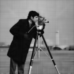
(a) “Cameraman”

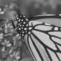
(b) “Butterfly”

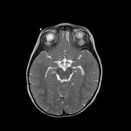
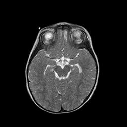
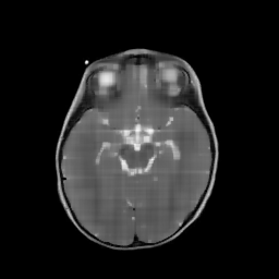
(c) “Brain”

Figure 4.1: Reconstruction of the three test images with $r$ chosen such that 4.2 holds true for $\alpha=0.1$: original image (left panel), noisy image (center), reconstructed image (right panel).

To cope with this, we applied the method with a smaller function $r$ (shifted by a constant) to prevent oversmoothing, see Figure 4.2. This implies that the statistical guarantee 4.3 is lost, but therefore the constraints are more restrictive and prevent oversmoothing. Note that a similar observation was made in [19]. It can be seen from Figure 4.2 that the corresponding reconstruction is less smooth, but seems superior over the one in Figure 1(a).

Figure 4.2: Reconstruction of the cameraman image with decreased $r$ to reduce oversmoothing.

To further analyze the convergence behavior of Algorithm 3.2 in the present setting, we also depict in Figure 4.3 the value of the smoothness promoting functional $f$ from 4.4, the percentage of violated constraints

$$\frac{\#\{B\in\mathcal{B}:\eta(Z_{B},u_{B})\leq r(|B|)\}}{\#\mathcal{B}},$$

and the maximum

$$\max_{B\in\mathcal{B}}\frac{\eta(Z_{B},u_{B})-r(|B|)}{r(|B|)}$$

as well as average

$$\frac{1}{\#\mathcal{B}}\sum_{B\in\mathcal{B}}\frac{\max(0,\eta(Z_{B},u_{B})-r(|B|))}{r(|B|)}$$

of the relative constraint violation over all $B\in\mathcal{B}$, associated with the experiments corresponding to Figure 1(a), respectively. It becomes clear that the function values of $f$ drop rapidly to a plateau. Only after updating the Lagrange multiplier estimate $v^{k}$ in iteration $k=2$, the value jumps up again as in the augmented Lagrangian function, the constraints are weighted higher in comparison to the functional $f$. The noisy behavior in the graph is clearly due to the usage of a stochastic gradient descent method, which, however, does not influence the long time behavior. The immediate decay of $f$, followed by an increase, also agrees with the number of fulfilled constraints. In the beginning, about $80$ percent of the constraints are violated as the Lagrange multiplier estimate is $0$ and, thus, the focus is on minimizing the functional $f$ without constraints. Exactly with updating the estimate $v^{k}$, the graph drops down such that in the end almost all constraints are fulfilled, indicating that the reconstruction is in fact a solution of 4.1.

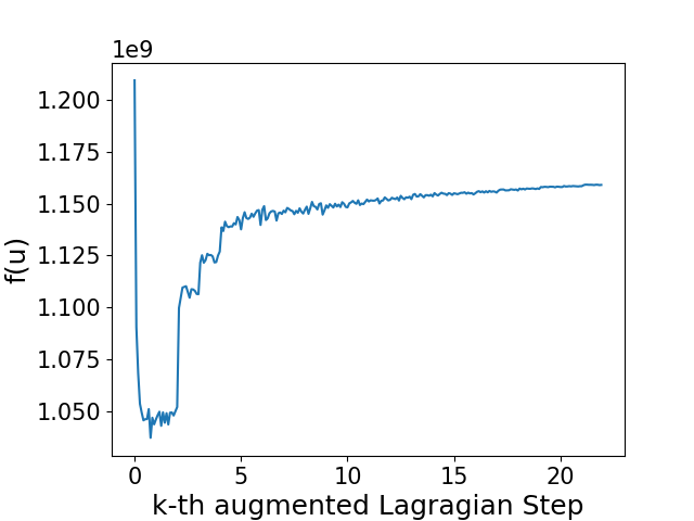
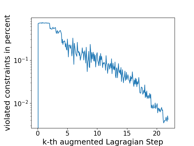
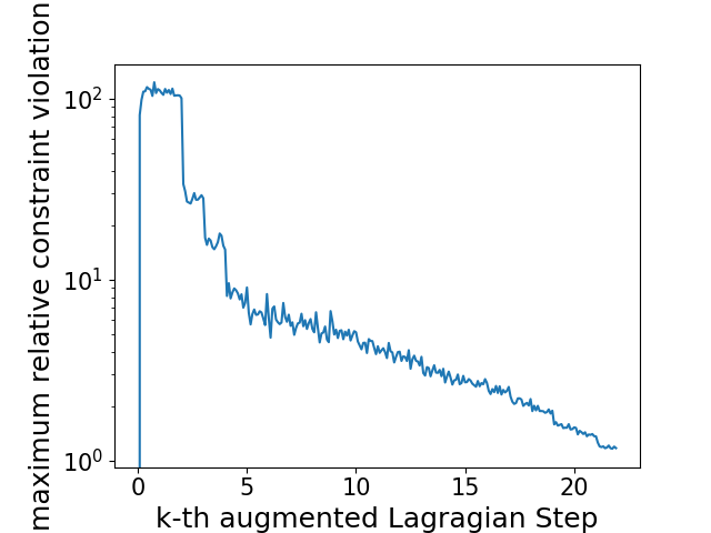
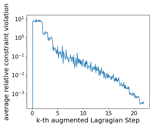
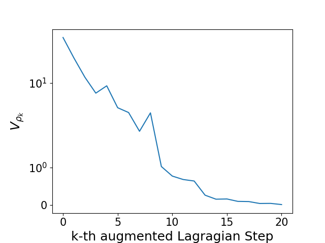
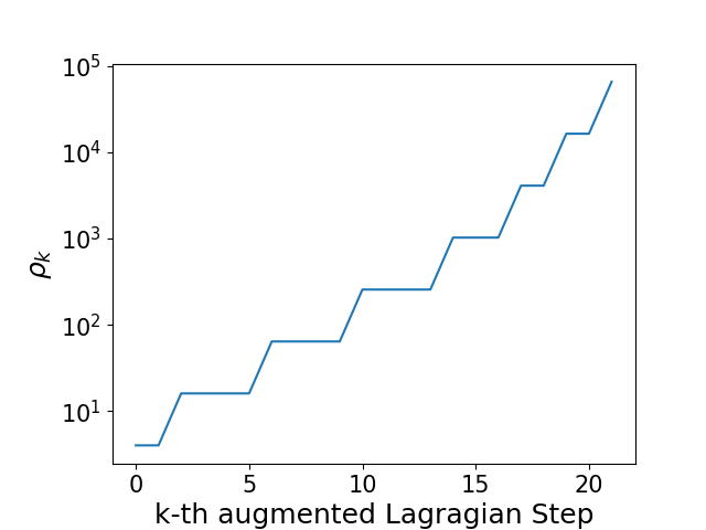
Figure 4.3: Convergence behavior of cameraman image with statistical $r$: number of iterations vs. objective function value (left upper panel), percentage of violated constraints (right upper panel), maximal relative constraint violation (left middle panel), average relative constraint violation (right middle panel), termination criterion from Remark 3.8 (left lower panel), penalty parameter (right lower panel).

5 Sparse Control

5.1 Description of the Problem

Let $\Omega\subset\mathbb{R}^{d}$ be a bounded open set and consider the optimal control problem

$$\min\limits_{y,u} \frac{1}{2}\left\|y-y_{\textup{d}}\right\|_{2}^{2}+\frac{\sigma}{2}\left\|u\right\|_{2}^{2}$$ (OC)

s.t. $$\mathopen{}-\Delta y=u$$

$$\left\|u\right\|_{1}\leq\kappa$$

$$y\in H^{1}_{0}(\Omega),\,u\in L^{2}(\Omega)$$

where $y_{\textup{d}}\in L^{2}(\Omega)$ is a desired state, $\sigma>0$ is a regularization parameter, and $\kappa>0$ is a constant which is used to model the desired level of sparsity of the optimal control function. The appearing elliptic PDE $-\Delta y=u$ has to be understood in the weak sense, i.e.,

$$\int_{\Omega}\nabla y^{\top}\nabla\phi\,\mathrm{d}\omega=\int_{\Omega}u\phi\,\mathrm{d}\omega\quad\forall\phi\in H^{1}_{0}(\Omega).$$

It is folklore that this variational problem possesses a unique solution in $H^{1}_{0}(\Omega)$ for each $u\in L^{2}(\Omega)$. Further, the associated solution operator is linear and continuous. It is well known that incorporating the $L^{1}$-norm of the control function into the objective function of an optimal control problem promotes sparsity of controls, i.e., the optimal control tends to vanish on large parts of the underlying domain. Here, we strike a different path to sparse controls by incorporating a hard sparsity constraint into a standard optimal control problem. A related approach to sparse control (in space) of parabolic equations can be found in the recent papers [10, 11]. It is easily seen that OC is a convex optimization problem which possesses a unique solution, see Remark 3.1 as well. Here, we aim to solve this problem numerically via the augmented Lagrangian method discussed in Section 3. Since the objective function is strongly convex (w.r.t. the control), the convergence result from Corollary 3.7 applies.

Therefore, we will augment the crucial cardinality constraint which we will interpret as a single scalar but nonsmooth inequality (and not as a geometric constraint enforcing that the control is in the $\kappa$-ball around $0$ w.r.t. the $L^{1}$-norm which might also be possible). Respecting this, for a given penalty parameter $\rho>0$ and some Lagrange multiplier estimate $v$, the augmented Lagrangian subproblem 3.2 takes the precise form

$$\min\limits_{y,u} \frac{1}{2}\left\|y-y_{\textup{d}}\right\|_{2}^{2}+\frac{\sigma}{2}\left\|u\right\|_{2}^{2}+\frac{1}{2\rho}\left(\max\nolimits^{2}\bigl{(}0,v+\rho(\left\|u\right\|_{1}-\kappa)\bigr{)}-v^{2}\right)$$ (5.1)

s.t. $$\mathopen{}-\Delta y=u$$

$$y\in H^{1}_{0}(\Omega),\,u\in L^{2}(\Omega),$$

and it is a convex optimization problem as well, see Example 2.2. The feasible set of 5.1 consists of all state-control pairs which satisfy the given PDE constraint. It is a closed subspace of $H^{1}_{0}(\Omega)\times L^{2}(\Omega)$. Particularly, it is weakly sequentially closed.

In the remainder of this section, we will first describe how 5.1 can be solved with the aid of a semismooth Newton method, see e.g. [13, 23, 26, 39, 45], in Section 5.2. Afterwards, we discuss the discretization of the subproblem 5.1 in Section 5.3. In Section 5.4, we comment on the implementation of the superordinate augmented Lagrangian method from Algorithm 3.2 for the actual numerical solution of OC before presenting illustrative results of numerical experiments.

5.2 Semismooth Newton Method as a Subproblem Solver

Let us reinspect the augmented Lagrangian subproblem 5.1 for fixed penalty parameter $\rho>0$ and multiplier estimate $v$. To start, observe that the quadratic regularization term in the objective function of this convex optimization problem guarantees that it possesses a unique minimizer. Next, we are going to characterize this minimizer with the aid of optimality conditions. Proceeding via the standard adjoint approach of optimal control, see e.g. [43], while exploiting a suitable chain rule (from nonsmooth analysis), see e.g. [34, Corollary 3.8], one can easily show that a pair $(\bar{y},\bar{u})\in H^{1}_{0}(\Omega)\times L^{2}(\Omega)$ is the minimizer of 5.1 if and only if there exists an adjoint state $\bar{p}\in H^{1}_{0}(\Omega)$ such that the following conditions are valid:

$$\bar{p}-\sigma\bar{u} \in\max\bigl{(}0,v+\rho(\left\|\bar{u}\right\|_{1}-\kappa)\bigr{)}\partial\left\|\cdot\right\|_{1}(\bar{u}),$$ (5.2)

$$-\Delta\bar{y} =\bar{u},$$

$$-\Delta\bar{p} =y_{\textup{d}}-\bar{y}.$$

The appearing subdifferential $\partial\left\|\cdot\right\|_{1}(\bar{u})$ can be easily computed as

$$\partial\left\|\cdot\right\|_{1}(\bar{u}):=\left\{\xi\in L^{2}(\Omega)\,\middle|\,\begin{aligned} \xi&=-1&&\text{a.e.\ on }\{\bar{u}<0\}\\ \xi&=1&&\text{a.e.\ on }\{\bar{u}>0\}\\ \xi&\in[-1,1]&&\text{a.e.\ on }\{\bar{u}=0\}\end{aligned}\right\},$$

see e.g. [25, Chapter 0.3.2]. We now aim to rewrite 5.2 as a system of nonsmooth equations. Therefore, we make use of the shrinkage operator $\mathcal{S}_{\sigma}\colon\mathbb{R}^{2}\to\mathbb{R}$ given by

$$\mathcal{S}_{\sigma}(a,b):=\max(0,(a-b_{+})/\sigma)+\min(0,(a+b_{+})/\sigma)\qquad\forall(a,b)\in\mathbb{R}^{2}$$

where we use $b_{+}:=\max(0,b)$ for brevity of notation. The precise definition of $\mathcal{S}_{\sigma}$ is not only motivated by our desire to reformulate the conditions from 5.2 in compact form, but it also turns out to be beneficial when invertibility issues in the context of the underlying semismooth Newton method are discussed. With the aid of $\mathcal{S}_{\sigma}$, we can rewrite 5.2 by means of the system

$$-\Delta\bar{p}+\bar{y}-y_{\textup{d}} =0,$$ (5.3)

$$\bar{u}-\mathcal{S}_{\sigma}(\bar{p},\bar{\beta}) =0,$$

$$-\Delta\bar{y}-\bar{u} =0,$$

$$\bar{\beta}-\max\bigl{(}0,v+\rho(\left\|\bar{u}\right\|_{1}-\kappa)\bigr{)} =0$$

in the unknown variables $(\bar{y},\bar{u},\bar{p},\bar{\beta})\in H^{1}_{0}(\Omega)\times L^{2}(\Omega)\times H^{1}_{0}(\Omega)\times\mathbb{R}$. The second equation, in which $\mathcal{S}_{\sigma}$ is evaluated in pointwise fashion, has to hold almost everywhere on $\Omega$.

As an abbreviation, we use $V:=H^{1}_{0}(\Omega)\times L^{2}(\Omega)\times H^{1}_{0}(\Omega)\times\mathbb{R}$, and introduce a residual mapping $F\colon V\to V^{*}$ by means of

$$F(z):=\begin{pmatrix}-\Delta p+y-y_{\textup{d}}\\ u-\mathcal{S}_{\sigma}(p,\beta)\\ -\Delta y-u\\ \beta-\max\bigl{(}0,v+\rho(\left\|u\right\|_{1}-\kappa)\bigr{)}\end{pmatrix}\qquad\forall z=(y,u,p,\beta)\in V.$$

Clearly, $\bar{z}\in V$ solves 5.3 if and only if $F(\bar{z})=0$, i.e., we need to find the roots of $F$. In order to apply the semismooth Newton method for this purpose, we need to clarify that $F$ is actually semismooth, its generalized derivative has to be determined, and, in order to guarantee local fast convergence, local uniform invertibility of the generalized derivative has to be investigated.

Let us start with the discussion of the semismoothness of $F$. This is not an issue for the first and third components as they are induced by continuous affine operators. As $H^{1}_{0}(\Omega)$ is continuously embedded in $L^{2+\delta}(\Omega)$ for some sufficiently small $\delta>0$ (depending on the dimension $d$), we can apply e.g. [23, Proposition 4.1] in order to obtain that the superposition operators associated with $\max(0,\cdot)$ and $\min(0,\cdot)$ are semismooth as mappings from $H^{1}_{0}(\Omega)$ to $L^{2}(\Omega)$. Hence, the second component of $F$ is semismooth as all remaining finite-dimensional operations are semismooth. Finally, observe that the superposition operator associated with $|\cdot|$ is semismooth as a mapping from $L^{2}(\Omega)$ to $L^{1}(\Omega)$, again due to [23, Proposition 4.1]. As integration is a continuous linear operation on $L^{1}(\Omega)$, $\left\|\cdot\right\|_{1}$ is a semismooth function from $L^{2}(\Omega)$ to $\mathbb{R}$. The remaining finite-dimensional operations in the last component of $F$ are semismooth as well.

With the aid of [23, Proposition 4.1] and suitable chain rules for semismooth compositions, see e.g. [45, Section 7], we are in position to characterize a suitable generalized derivative of $F$ which can be used in the semismooth Newton method. These results show that

$$F^{\prime}(z):=\begin{pmatrix}\mathcal{I}^{*}\mathcal{I}&0&-\Delta&0\\ 0&\operatorname{id}_{L^{2}(\Omega)}&-\sigma^{-1}D_{I}\mathcal{I}&\sigma^{-1}\theta_{1}(\chi_{I_{1}}-\chi_{I_{2}})\\ -\Delta&-\mathcal{I}^{*}&0&0\\ 0&-\rho\theta_{2}\operatorname{Sign}_{u}&0&1\end{pmatrix}$$ (5.4)

serves as a generalized derivative of $F$ at $z=(y,u,p,\beta)\in V$. Above, $\mathcal{I}\colon H^{1}_{0}(\Omega)\to L^{2}(\Omega)$ denotes the canonical injection of $H^{1}_{0}(\Omega)$ into $L^{2}(\Omega)$, and its adjoint $\mathcal{I}^{*}\colon L^{2}(\Omega)\to H^{-1}(\Omega)$ is the canonical injection of $L^{2}(\Omega)$ into $H^{-1}(\Omega)$ (note that we identify $L^{2}(\Omega)$ and its dual with each other). We made use of the index sets

$$I_{1}:=\{p-\beta_{+}>0\},\qquad I_{2}:=\{p+\beta_{+}<0\},\qquad I:=I_{1}\cup I_{2}.$$

Furthermore, $D_{I}\colon L^{2}(\Omega)\to L^{2}(\Omega)$ denotes the pointwise multiplication with $\chi_{I}$, and $\operatorname{Sign}_{u}\colon L^{2}(\Omega)\to\mathbb{R}$ is given by

$$\operatorname{Sign}_{u}(\tilde{u}):=(\operatorname{sign}(u),\tilde{u})_{2}\qquad\forall\tilde{u}\in L^{2}(\Omega),$$

where we used $(\cdot,\cdot)_{2}\colon L^{2}(\Omega)\times L^{2}(\Omega)\to\mathbb{R}$ in order to denote the standard inner product in the Hilbert space $L^{2}(\Omega)$ for brevity of notation. Finally, we made use of

$$\theta_{1}:=\begin{cases}0&\text{if }\beta<0,\\ 1&\text{if }\beta\geq 0,\end{cases}\qquad\theta_{2}:=\begin{cases}0&\text{if }v+\rho(\left\|u\right\|_{1}-\kappa)<0,\\ 1&\text{if }v+\rho(\left\|u\right\|_{1}-\kappa)\geq 0.\end{cases}$$

In the subsequent result, we show local uniform invertibility of the derivative from 5.4 under an additional assumption.

Lemma 5.1.

There exists a constant $c>0$, such that for all $z=(y,u,p,\beta)\in V$ with $u>0$ a.e. on $I_{1}$ and $u<0$ a.e. on $I_{2}$, the operator $F^{\prime}(z)$ is invertible with $\left\|F^{\prime}(z)^{-1}\right\|\leq c$.

Proof: Fix $z=(y,u,p,\beta)\in V$ such that $I_{1}\subset\{u>0\}$ and $I_{2}\subset\{u<0\}$. Let a right-hand side $r=(r_{1},r_{2},r_{3},r_{4})\in V^{*}$ be given. We have to find $d=(d_{1},d_{2},d_{3},d_{4})\in V$ with $F^{\prime}(z)d=r$, i.e.,

$$\begin{pmatrix}\mathcal{I}^{*}\mathcal{I}&0&-\Delta&0\\ 0&\operatorname{id}_{L^{2}(\Omega)}&-\sigma^{-1}D_{I}\mathcal{I}&\sigma^{-1}\theta_{1}(\chi_{I_{1}}-\chi_{I_{2}})\\ -\Delta&-\mathcal{I}^{*}&0&0\\ 0&-\rho\theta_{2}\operatorname{Sign}_{u}&0&1\end{pmatrix}\begin{pmatrix}d_{1}\\ d_{2}\\ d_{3}\\ d_{4}\end{pmatrix}=\begin{pmatrix}r_{1}\\ r_{2}\\ r_{3}\\ r_{4}\end{pmatrix}.$$

Now, we multiply the first equation (from the left) by $\sigma^{-1}D_{I}\mathcal{I}(-\Delta)^{-1}$ and the third equation (from the left) by $-\sigma^{-1}D_{I}\mathcal{I}(-\Delta)^{-1}\mathcal{I}^{*}\mathcal{I}(-\Delta)^{-1}$ and add everything to the second equation. By only considering the second and fourth equation, this gives

$$\begin{pmatrix}\operatorname{id}_{L^{2}(\Omega)}+\sigma^{-1}D_{I}\mathcal{Q}\mathcal{Q}&\sigma^{-1}\theta_{1}(\chi_{I_{1}}-\chi_{I_{2}})\\ -\rho\theta_{2}\operatorname{Sign}_{u}&1\end{pmatrix}\begin{pmatrix}d_{2}\\ d_{4}\end{pmatrix}=\begin{pmatrix}r_{5}\\ r_{4}\end{pmatrix}.$$ (5.5)

with the self-adjoint operator $\mathcal{Q}:=\mathcal{I}(-\Delta)^{-1}\mathcal{I}^{*}\colon L^{2}(\Omega)\to L^{2}(\Omega)$ and

$$r_{5}:=r_{2}+\sigma^{-1}D_{I}\mathcal{I}(-\Delta)^{-1}r_{1}-\sigma^{-1}D_{I}\mathcal{I}(-\Delta)^{-1}\mathcal{I}^{*}\mathcal{I}(-\Delta)^{-1}r_{3}.$$

It is well known that the operator $\operatorname{id}_{L^{2}(\Omega)}+\sigma^{-1}D_{I}\mathcal{Q}\mathcal{Q}$ from $L^{2}(\Omega)$ into itself is invertible with

$$\left(\operatorname{id}_{L^{2}(\Omega)}+\sigma^{-1}D_{I}\mathcal{Q}\mathcal{Q}\right)^{-1}=\operatorname{id}_{L^{2}(\Omega)}-\sigma^{-1}D_{I}\mathcal{Q}\left(\operatorname{id}_{L^{2}(\Omega)}+\sigma^{-1}\mathcal{Q}D_{I}\mathcal{Q}\right)^{-1}\mathcal{Q}.$$

Since $\mathcal{Q}$ is self-adjoint, we can use the Lax–Milgram Lemma to show that

$$\left\|(\operatorname{id}_{L^{2}(\Omega)}+\sigma^{-1}\mathcal{Q}D_{I}\mathcal{Q})^{-1}\right\|\leq 1,$$

and together with the fact that the operator norm of $D_{I}$ is bounded from above by $1$, we find the uniform bound

$$\left\|(\operatorname{id}_{L^{2}(\Omega)}+\sigma^{-1}D_{I}\mathcal{Q}\mathcal{Q})^{-1}\right\|\leq 1+\sigma^{-1}\left\|\mathcal{Q}\right\|^{2},$$

see, e.g., [35, Lemma 3.14] or [22] for a different proof. Thus, we can consider a Schur complement in 5.5 and arrive at

$$\left(1+\frac{\rho\theta_{1}\theta_{2}}{\sigma}\operatorname{Sign}_{u}(\operatorname{id}_{L^{2}(\Omega)}+\sigma^{-1}D_{I}\mathcal{Q}\mathcal{Q})^{-1}(\chi_{I_{1}}-\chi_{I_{2}})\right)d_{4}=r_{6}$$ (5.6)

with

$$r_{6}:=r_{4}+\rho\theta_{2}\operatorname{Sign}_{u}(\operatorname{id}_{L^{2}(\Omega)}+\sigma^{-1}D_{I}\mathcal{Q}\mathcal{Q})^{-1}r_{5}.$$ (5.7)

Note that equation 5.6 lives in $\mathbb{R}$. In order to prove its stable solvability, we check that the number

$$\theta_{1}\operatorname{Sign}_{u}(\operatorname{id}_{L^{2}(\Omega)}+\sigma^{-1}D_{I}\mathcal{Q}\mathcal{Q})^{-1} (\chi_{I_{1}}-\chi_{I_{2}})$$

$$=(\operatorname{sign}(u),\theta_{1}(\operatorname{id}_{L^{2}(\Omega)}+\sigma^{-1}D_{I}\mathcal{Q}\mathcal{Q})^{-1}(\chi_{I_{1}}-\chi_{I_{2}}))_{2}$$

is non-negative. As this is trivially satisfied for $\theta_{1}=0$, let us assume that $\theta_{1}=1$, i.e., $\beta\geq 0$. We set

$$\tilde{u}:=(\operatorname{id}_{L^{2}(\Omega)}+\sigma^{-1}D_{I}\mathcal{Q}\mathcal{Q})^{-1}(\chi_{I_{1}}-\chi_{I_{2}}),$$

i.e.,

$$\chi_{I_{1}}-\chi_{I_{2}}=(\operatorname{id}_{L^{2}(\Omega)}+\sigma^{-1}D_{I}\mathcal{Q}\mathcal{Q})\tilde{u}.$$

Since $D_{I}$ is the pointwise multiplication with $\chi_{I}$, this shows that $\tilde{u}$ vanishes outside of $I$. The assumptions on $u$ guarantee $\operatorname{sign}(u)\chi_{I}=\chi_{I_{1}}-\chi_{I_{2}}$. Thus,

$$(\operatorname{sign}(u),\tilde{u})_{2} =(\operatorname{sign}(u)\chi_{I},\tilde{u})_{2}=(\chi_{I_{1}}-\chi_{I_{2}},\tilde{u})_{2}$$

$$=((\operatorname{id}_{L^{2}(\Omega)}+\sigma^{-1}D_{I}\mathcal{Q}\mathcal{Q})\tilde{u},\tilde{u})_{2}$$

$$=((\operatorname{id}_{L^{2}(\Omega)}+\sigma^{-1}D_{I}\mathcal{Q}\mathcal{Q}D_{I})\tilde{u},\tilde{u})_{2}\geq 0.$$

In order to finish the proof, we solve the above systems in reverse order. First, we set

$$d_{4}:=\left(1+\frac{\rho\theta_{1}\theta_{2}}{\sigma}\operatorname{Sign}_{u}(\operatorname{id}_{L^{2}(\Omega)}+\sigma^{-1}D_{I}\mathcal{Q}\mathcal{Q})^{-1}(\chi_{I_{1}}-\chi_{I_{2}})\right)^{-1}r_{6}$$

in order to satisfy 5.6, and we have

$$\left|d_{4}\right|\leq\left|r_{6}\right|\leq\left|r_{4}\right|+c_{1}\left\|r_{5}\right\|_{2}$$

from 5.7 for some constant $c_{1}>0$ which is independent of $z$ as the operator norm of $\operatorname{Sign}_{u}$ is bounded from above by $\sqrt{\left|\Omega\right|}$. Similarly, the definition of $r_{5}$ gives

$$\left\|r_{5}\right\|_{2}\leq c_{2}\left\|r\right\|_{V^{*}}$$

for some constant $c_{2}>0$ independent of $z$. Hence, $\left|d_{4}\right|\leq c_{3}\left\|r\right\|_{V^{*}}$ for some constant $c_{3}>0$ independent of $z$. Next, we set

$$d_{2}:=\left(\operatorname{id}_{L^{2}(\Omega)}+\sigma^{-1}D_{I}\mathcal{Q}\mathcal{Q}\right)^{-1}\left(r_{5}-\sigma^{-1}\theta_{1}d_{4}(\chi_{I_{1}}-\chi_{I_{2}})\right).$$

Again, $\left\|d_{2}\right\|_{2}\leq c_{4}\left\|r\right\|_{V^{*}}$ for some constant $c_{4}>0$ independent of $z$. Finally, we set

$$d_{1}:=(-\Delta)^{-1}(r_{3}+\mathcal{I}^{*}d_{2}),\qquad d_{3}:=(-\Delta)^{-1}(r_{1}-\mathcal{I}^{*}\mathcal{I}d_{1})$$

and we have $F^{\prime}(z)d=r$ by construction. By combining the above estimates, we get $\left\|d\right\|_{V}\leq c\left\|r\right\|_{V^{*}}$ for some constant $c>0$ independent of $z$. $\Box$

In Algorithm 5.2, we now state a semismooth Newton method for the computational solution of 5.1.

Algorithm 5.2 (Local Semismooth Newton Method for 5.1).

1:$(y^{0},p^{0},\beta_{0})\in H^{1}_{0}(\Omega)\times H^{1}_{0}(\Omega)\times\mathbb{R}$, parameter $\varepsilon^{\textup{ssn}}_{\textup{abs}}\geq 0$

2:Set $\ell:=0$.

3:Set $u^{0}:=\mathcal{S}_{\sigma}(p^{0},\beta_{0})$ and $z^{0}:=(y^{0},u^{0},p^{0},\beta_{0})$.

4:while $\|F(z^{\ell})\|_{V^{*}}>\varepsilon^{\textup{ssn}}_{\textup{abs}}$ do

5:     Compute the solution $\delta z^{\ell+1}:=(\delta y^{\ell+1},\delta u^{\ell+1},\delta p^{\ell+1},\delta\beta_{\ell+1})\in V$ of

$$F^{\prime}(z^{\ell})\delta z=-F(z^{\ell}).$$

6:     Set $\tilde{z}^{\ell+1}:=z^{\ell}+\delta z^{\ell}$.

7:     Set $u^{\ell+1}:=\mathcal{S}_{\sigma}(\tilde{p}^{\ell+1},\tilde{\beta}_{\ell+1})$ and $z^{\ell+1}:=(\tilde{y}^{\ell+1},u^{\ell+1},\tilde{p}^{\ell+1},\tilde{\beta}_{\ell+1})$.

8:     Set $\ell\leftarrow\ell+1$.

9:end while

10:return $z^{\ell}$

Let us comment on the rather uncommon 3 and 7 in Algorithm 5.2. Therefore, fix an iteration $\ell\in\mathbb{N}$ as well as an iterate $z^{\ell}=(y^{\ell},u^{\ell},p^{\ell},\beta_{\ell})\in V$ of Algorithm 5.2. The aforementioned additional application of the shrinkage operator gives $u^{\ell}=\mathcal{S}_{\sigma}(p^{\ell},\beta_{\ell})$ almost everywhere on $\Omega$, and this guarantees that $u^{\ell}>0$ almost everywhere on $\{p^{\ell}-(\beta_{\ell})_{+}>0\}$ and $u^{\ell}<0$ almost everywhere on $\{p^{\ell}+(\beta_{\ell})_{+}<0\}$. Now, due to Lemma 5.1, it is clear that the generalized derivative $F^{\prime}(z^{\ell})$ is invertible and, thus, 5 is well defined.

Classical convergence results for semismooth Newton methods in function spaces show that, if the method is initialized in a sufficiently small neighborhood of a solution where the generalized derivative is locally nonsingular and uniformly invertible, then the computed sequence converges superlinearly to this solution, see e.g. [23, Theorem 1.1]. Let us point out that, due to the presence of 3 and 7, Algorithm 5.2 is seemingly not a semismooth Newton method in the narrower sense. However, in our next result, we will demonstrate that Algorithm 5.2 corresponds to a semismooth Newton method applied to a reduced version of the system 5.3, so that we can rely on the aforementioned classical finding.

To this end, set $\widetilde{V}:=H^{1}_{0}(\Omega)\times H^{1}_{0}(\Omega)\times\mathbb{R}$ and consider $\widetilde{F}\colon\widetilde{V}\to\widetilde{V}^{*}$ given by

$$\widetilde{F}(\tilde{z}):=\begin{pmatrix}-\Delta p+y-y_{\textup{d}},\\ -\Delta y-\mathcal{S}_{\sigma}(p,\beta),\\ \beta-\max\bigl{(}0,v+\rho(\|\mathcal{S}_{\sigma}(p,\beta)\|_{1}-\kappa)\bigr{)}\end{pmatrix}\qquad\forall\tilde{z}=(y,p,\beta)\in\widetilde{V}.$$

Using similar arguments as above, we can easily check that $\widetilde{F}$ is semismooth, and that

$$\widetilde{F}^{\prime}(\tilde{z}):=\begin{pmatrix}\mathcal{I}^{*}\mathcal{I}&-\Delta&0\\ -\Delta&-\sigma^{-1}\mathcal{I}^{*}D_{I}\mathcal{I}&\sigma^{-1}\theta_{1}\mathcal{I}^{*}(\chi_{I_{1}}-\chi_{I_{2}})\\ 0&-\rho\sigma^{-1}\tilde{\theta}_{2}\mathcal{J}_{I_{1},I_{2}}&1+\rho\sigma^{-1}\theta_{1}\tilde{\theta}_{2}(|I_{1}|+|I_{2}|)\end{pmatrix}$$ (5.8)

serves as a generalized derivative of $\widetilde{F}$ at $\tilde{z}=(y,p,\beta)\in\widetilde{V}$. Above, we used $\mathcal{J}_{I_{1},I_{2}}\colon H^{1}_{0}(\Omega)\to\mathbb{R}$ given by

$$\forall\tilde{p}\in H^{1}_{0}(\Omega)\colon\quad\mathcal{J}_{I_{1},I_{2}}(\tilde{p}):=(\mathcal{I}\tilde{p},\chi_{I_{1}}-\chi_{I_{2}})_{2},$$

and

$$\tilde{\theta}_{2}:=\begin{cases}0&\text{if }v+\rho(\|\mathcal{S}_{\sigma}(p,\beta)\|_{1}-\kappa)<0,\\ 1&\text{if }v+\rho(\|\mathcal{S}_{\sigma}(p,\beta)\|_{1}-\kappa)\geq 0.\end{cases}$$

Furthermore, let us point out that

$$-\rho\sigma^{-1}\tilde{\theta}_{2}\mathcal{J}_{I_{1},I_{2}} =-\rho\sigma^{-1}\tilde{\theta}_{2}\bigl{(}\operatorname{Sign}_{\mathcal{S}_{\sigma}(p,\beta)}D_{I}\mathcal{I}),$$ (5.9)

$$\rho\sigma^{-1}\theta_{1}\tilde{\theta}_{2}(|I_{1}|+|I_{2}|) =-\rho\tilde{\theta}_{2}\operatorname{Sign}_{\mathcal{S}_{\sigma}(p,\beta)}\bigl{(}\sigma^{-1}\theta_{1}(-\chi_{I_{1}}+\chi_{I_{2}})\bigr{)},$$

see 5.4 as well.

Lemma 5.3.

Fix $z=(y,u,p,\beta)\in V$ such that $u=\mathcal{S}_{\sigma}(p,\beta)$ and set $\tilde{z}:=(y,p,\beta)$.

1. We have $\|F(z)\|_{V^{*}}=\|\widetilde{F}(\tilde{z})\|_{\widetilde{V}^{*}}$.

2. If the quadruple $\delta z=(\delta y,\delta u,\delta p,\delta\beta)\in V$ solves

   $$F^{\prime}(z)\delta z=-F(z),$$ (5.10)

   then the triplet $\widetilde{\delta z}:=(\delta y,\delta p,\delta\beta)\in\widetilde{V}$ solves

   $$\widetilde{F}^{\prime}(\tilde{z})\widetilde{\delta z}=-\widetilde{F}(\tilde{z}).$$ (5.11)

3. If the triplet $\widetilde{\delta z}=(\delta y,\delta p,\delta\beta)\in\widetilde{V}$ solves 5.11, then the quadruple $\delta z:=(\delta y,\delta u,\delta p,\delta\beta)\in V$ with $\delta u:=\sigma^{-1}(D_{I}\mathcal{I})\delta p-\sigma^{-1}\theta_{1}\delta\beta(\chi_{I_{1}}-\chi_{I_{2}})$ solves 5.10.

Proof: The proof of the first assertion is obvious by definition of $F$ and $\widetilde{F}$ due to $u=\mathcal{S}_{\sigma}(p,\beta)$.

For the proof of the second statement, we fix a solution $\delta z:=(\delta y,\delta u,\delta p,\delta\beta)\in V$ of 5.10. The first equation in 5.10 and 5.11 coincide. Note that the second equation of 5.10 gives

$$\delta u=\sigma^{-1}(D_{I}\mathcal{I})\delta p-\sigma^{-1}\theta_{1}\delta\beta(\chi_{I_{1}}-\chi_{I_{2}})$$

as $u-\mathcal{S}_{\sigma}(p,\beta)=0$. Hence, we find

$$-\Delta\delta y-\sigma^{-1}(\mathcal{I}^{*}D_{I}\mathcal{I})\delta p+\sigma\theta_{1}\delta\beta\mathcal{I}^{*}(\chi_{I_{1}}-\chi_{I_{2}})=-\Delta\delta y-\mathcal{I}^{*}\delta u=-\Delta y-u,$$

i.e., the second equation of 5.11 holds. Similarly, respecting 5.9 yields

$$-\rho\sigma^{-1}\tilde{\theta}_{2}\mathcal{J}_{I_{1},I_{2}}\delta p+(1+\rho\sigma^{-1}\theta_{1}\tilde{\theta}_{2}(|I_{1}|+|I_{2}|))\delta\beta$$

$$\qquad=-\rho\theta_{2}\operatorname{Sign}_{u}(\sigma^{-1}(D_{I}\mathcal{I})\delta p)+\bigl{(}1-\rho\theta_{2}\operatorname{Sign}_{u}\bigl{(}\sigma^{-1}\theta_{1}(-\chi_{1}+\chi_{I_{2}})\bigr{)}\bigr{)}\delta\beta$$

$$\qquad=-\rho\theta_{2}\operatorname{Sign}_{u}\bigl{(}\delta u+\sigma^{-1}\theta_{1}\delta\beta(\chi_{I_{1}}-\chi_{I_{2}})\bigr{)}+\bigl{(}1-\rho\theta_{2}\operatorname{Sign}_{u}\bigl{(}\sigma^{-1}\theta_{1}(-\chi_{1}+\chi_{I_{2}})\bigr{)}\bigr{)}\delta\beta$$

$$\qquad=-\rho\theta_{2}\operatorname{Sign}_{u}\delta u+\delta\beta$$

$$\qquad=\beta-\max\bigl{(}0,v+\rho(\left\|u\right\|_{1}-\kappa)\bigr{)}=\beta-\max\bigl{(}0,v+\rho(\|\mathcal{S}_{\sigma}(p,\beta)\|_{1}-\kappa)\bigr{)},$$

i.e., the third equation of 5.11 holds. Hence, $\widetilde{\delta z}$ is a solution of 5.11.

The proof of the final assertion is completely analogous. $\Box$

The above lemma gives rise to the following corollary.

Corollary 5.4.

1. Combining Lemmas 5.1 and 5.3, we find that the linear operators 5.8 are uniformly invertible on $\widetilde{V}$.

2. Algorithm 5.2 precisely corresponds to the application of the standard semismooth Newton method for the solution of $\widetilde{F}(\tilde{z})=0$ based on the generalized derivative given in 5.8 initialized at $(y^{0},p^{0},\beta_{0})$ with termination criterion $\|\widetilde{F}(\tilde{z}^{\ell})\|_{\widetilde{V}^{*}}\leq\varepsilon_{\textup{eps}}$.

Taking into account that the superposition operators associated with $\max(0,\cdot)$ and $\min(0,\cdot)$, mapping from $L^{2}(\Omega)$ to itself, are Lipschitz continuous with Lipschitz modulus one, the superposition operator associated with $\mathcal{S}_{\sigma}$ is Lipschitz continuous as a mapping from $H^{1}_{0}(\Omega)\times\mathbb{R}$ to $L^{2}(\Omega)$ with Lipschitz modulus $\sigma^{-1}$. Furthermore, for each quadruple $z=(y,u,p,\beta)\in V$, $\left\|z\right\|_{V}\geq\|\tilde{z}\|_{\widetilde{V}}$ trivially holds for the triplet $\tilde{z}:=(y,p,\beta)\in\widetilde{V}$. Together with [23, Theorem 1.1] and Corollary 5.4, we obtain the following convergence result.

Theorem 5.5.

Let $(\bar{y},\bar{u})\in H^{1}_{0}(\Omega)\times L^{2}(\Omega)$ be the uniquely determined minimizer of 5.1, let $\bar{p}\in H^{1}_{0}(\Omega)$ be the uniquely determined associated adjoint state according to 5.2, and set $\bar{\beta}:=\max\bigl{(}0,v+\rho(\|\bar{u}\|_{1}-\kappa)\bigr{)}$. Whenever $(y^{0},p^{0},\beta_{0})\in H^{1}_{0}(\Omega)\times H^{1}_{0}(\Omega)\times\mathbb{R}$ is chosen sufficiently close to $(\bar{y},\bar{p},\bar{\beta})$ while Algorithm 5.2 started at $(y^{0},p^{0},\beta_{0})$ does not terminate due to 4, then the computed sequence $\{(y^{k},u^{k},p^{k},\beta_{k})\}\subset V$ converges superlinearly to $(\bar{y},\bar{u},\bar{p},\bar{\beta})$.

5.3 Discretization

The problem OC is discretized by a standard finite element approach. That is, we choose a triangulation of $\Omega$, and the variables $y$ and $u$ as well as the adjoint state $p$ are discretized by piecewise linear and continuous functions. The nodal basis functions are denoted by $\psi_{i}$, $i=1,\ldots,N$. The discretized counterparts of $y$, $u$, and $p$ will be denoted by $y_{h}$, $u_{h}$, and $p_{h}$, respectively. We introduce the stiffness matrix, the mass matrix, and a lumped mass matrix via

$$\mathcal{K}:=\left(\int_{\Omega}\nabla\psi_{i}^{\top}\nabla\psi_{j}\,\mathrm{d}\omega\right)_{i,j=1}^{N},\;\mathcal{M}:=\left(\int_{\Omega}\psi_{i}\psi_{j}\,\mathrm{d}\omega\right)_{i,j=1}^{N},\;\mathcal{M}_{L}:=\operatorname{diag}\left(\int_{\Omega}\psi_{i}\,\mathrm{d}\omega\right)_{i=1}^{N},$$

respectively. Since the functions $\psi_{i}$, $i=1,\ldots,N$, are non-negative, the diagonal of $\mathcal{M}_{L}$ is strictly positive and, thus, $\mathcal{M}_{L}$ is invertible. We discretize problem OC as

$$\min\limits_{y_{h},u_{h}} \frac{1}{2}(y_{h}-y_{\textup{d},h})^{\top}\mathcal{M}(y_{h}-y_{\textup{d},h})+\frac{\sigma}{2}u_{h}^{\top}\mathcal{M}_{L}u_{h}$$ (OC_h)

s.t. $$\mathopen{}\mathcal{K}y_{h}=\mathcal{M}_{L}u_{h}$$

$$e^{\top}\mathcal{M}_{L}\left|u_{h}\right|\leq\kappa$$

$$y_{h},u_{h}\in\mathbb{R}^{N}.$$

Here, $y_{\textup{d},h}$ is the interpolation of the desired state and $e\in\mathbb{R}^{N}$ is the all-ones vector. The use of the lumped mass matrices yields that the part of the optimality system of OC_h corresponding to the control can be interpreted coefficientwise. Consequently, it can again be rewritten by using a shrinkage operator. For the use of mass lumping for higher-order finite elements and for further references, we refer to [38].

In order to solve OC_h, we augment the sparsity constraint in the objective via an additional summand as in 5.1. Noting that $e^{\top}|u_{h}|=\left\|u_{h}\right\|_{1}$ holds for all $u_{h}\in\mathbb{R}^{N}$, the optimality system of this augmented Lagrangian subproblem is given by

$$\bar{p}_{h}-\sigma\bar{u}_{h} \in\max\bigl{(}0,v+\rho(e^{\top}\mathcal{M}_{L}\left|\bar{u}_{h}\right|-\kappa)\bigr{)}\partial\left\|\cdot\right\|_{1}(\bar{u}_{h}),$$ (5.12a)

$$\mathcal{K}\bar{y}_{h} =\mathcal{M}_{L}\bar{u}_{h},$$ (5.12b)

$$\mathcal{K}\bar{p}_{h} =\mathcal{M}(y_{\textup{d},h}-\bar{y}_{h}).$$ (5.12c)

Note that we already have canceled out the matrix $\mathcal{M}_{L}$ in 5.12a. Since 5.12 is a discretized version of 5.2, we can use the same steps as in Section 5.2 to arrive at a semismooth Newton method for its numerical solution.

5.4 Implementation and Numerical Results

We implemented Algorithm 3.2 for the numerical solution of the sparsity-constrained optimization problem OC in MATLAB2022b. The parameters in Algorithm 3.2 are chosen as $\rho_{0}:=10^{-4}$, $\tau:=0.1$, and $\gamma:=2$. Furthermore, we exploit $\lambda^{0}:=0$. The Lagrange multiplier estimate $v^{k}$ is chosen to be the projection of $\lambda^{k}$ onto the interval $[0,10^{8}]$ in 4 of Algorithm 3.2. Additionally, we made use of the termination criterion from Remark 3.8 with $\varepsilon^{\textup{alm}}_{\textup{abs}}:=10^{-6}$. In order to construct the starting point $x^{0}=(y^{0},u^{0})$ of Algorithm 3.2, we chose $y^{0}\equiv 0$. Furthermore, $p^{0}$ is the associated adjoint state, and $\beta_{0}:=10^{-6}$ is used to set $u^{0}:=\mathcal{S}_{\sigma}(p^{0},\beta_{0})$. The triplet $(y^{0},p^{0},\beta_{0})$ is also used to initialize the subproblem solver Algorithm 5.2 in the first iteration of Algorithm 3.2. For termination of Algorithm 5.2, we made use of $\varepsilon_{\textup{abs}}^{\textup{ssn}}:=10^{-6}\,2^{-k}$ in the $k$-th iteration of Algorithm 3.2. Note that, in each iteration $k\geq 1$ of Algorithm 3.2, we exploited the quadruple computed in the prior iteration $k-1$ to initialize Algorithm 5.2 in a canonical way.

The instance of problem OC we are considering for our numerical experiments is given on the unit square $\Omega:=(0,1)^{2}\subset\mathbb{R}^{2}$. The desired state $y_{\textup{d}}\colon\Omega\to\mathbb{R}$ is chosen as

$$y_{\textup{d}}(\omega):=\sin(\pi\omega_{1})\operatorname{exp}(\omega_{2})\qquad\forall\omega=(\omega_{1},\omega_{2})\in\Omega.$$

Note that, as $y\in H^{1}_{0}(\Omega)$ has to be chosen in OC, this desired state is not reachable. Furthermore, $\sigma:=10^{-2}$ is fixed. In order to discretize the problem, $\Omega$ has been triangulated by a uniform mesh of $2^{11}$ triangles. Figure 5.1 illustrates solutions of OC (or, more precisely, of the discretized problem OC_h) obtained for the four different sparsity parameters $\kappa\in\{100,10,2,0.5\}$. Let us note that the sparsity constraint is not active for the solution found for $\kappa=100$, i.e., this setting illustrates how the solution of OC looks like in situations where no sparsity constraint is present. In all four scenarios, the subproblem solver Algorithm 5.2 found a reasonable solution of the associated augmented Lagrangian subproblem 5.1. Thus, the local convergence guarantees from Theorem 5.5 already seemed to be enough for a satisfying behavior of the method, and the incorporation of an additional globalization technique in the semismooth Newton framework became completely superfluous.

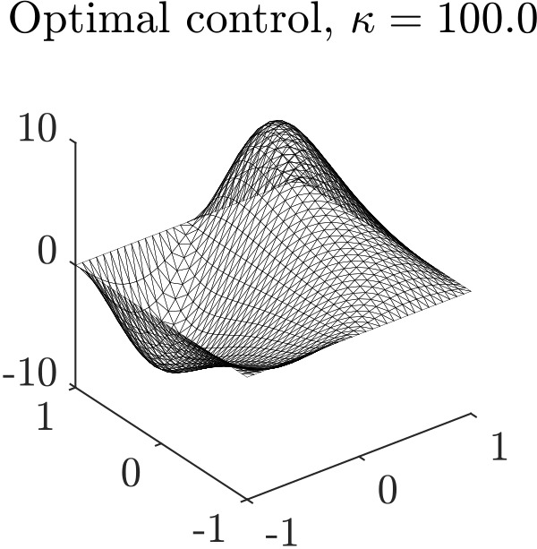
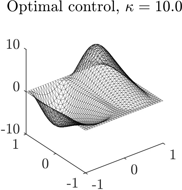
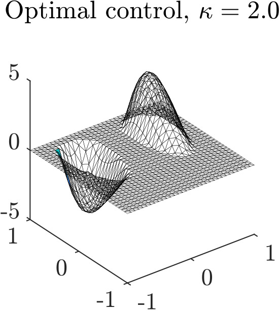
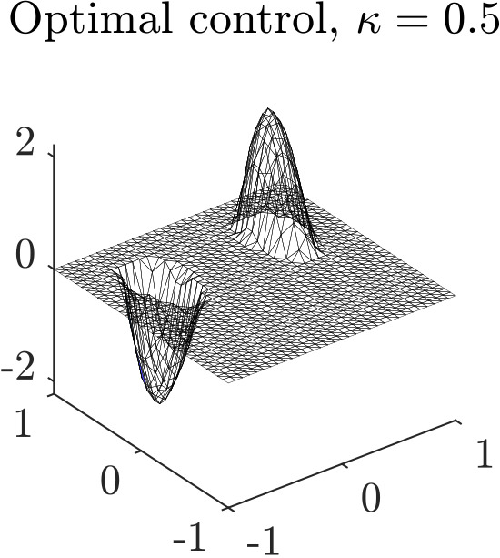
Figure 5.1: Optimal controls for OC for the different values $\kappa=100$, $\kappa=10$, $\kappa=2$, and $\kappa=0.5$ of the sparsity parameter.

In Table 5.1, we monitor some more precise numbers which document the behavior of Algorithm 3.2 for the particular choice $\kappa=0.5$ which is the most challenging setting. We observe that a maximum of $3$ iterations of the semismooth Newton method from Algorithm 5.2 is necessary in order to solve the augmented Lagrangian subproblem in each (outer) iteration of Algorithm 3.2. Throughout the whole run, $V_{\rho_{k}}(x^{k+1},v^{k})$ is monotonically decreasing, and after 16 iterations, falls below the threshold $\varepsilon_{\textup{abs}}^{\textup{alm}}$. The penalty parameter is enlarged 12 times throughout the run, but stays constant (and, still, comparatively small) throughout the last three iterations. We also note that this behavior is caused, on the one hand, since $\rho_{0}$ is comparatively small and, on the other hand, by our rather excessive choice of the parameter $\tau$. Exemplary, for $\rho_{0}:=0.01$ and $\tau:=0.9$, Algorithm 3.2 needs $44$ (outer) iterations to solve OC for $\kappa=0.5$, and the penalty parameter stays constant throughout the whole run.

$k$	$\ell$	$\rho_{k}$	$V_{\rho_{k}}(x^{k+1},v^{k})$
0	2	1.00e-4	1.135259e+1
1	2	1.00e-4	1.106969e+1
2	2	2.00e-4	1.054008e+1
3	2	4.00e-4	9.625707e+0
4	3	8.00e-4	8.220058e+0
5	3	1.60e-3	6.408010e+0
6	3	3.20e-3	4.402918e+0
7	3	6.40e-3	2.589087e+0
8	3	1.28e-2	1.271296e+0
9	3	2.56e-2	4.984998e-1
10	3	5.12e-2	1.453159e-1
11	3	1.02e-1	2.766288e-2
12	2	2.05e-1	3.082315e-3
13	2	4.10e-1	1.828053e-4
14	1	4.10e-1	1.087269e-5
15	1	4.10e-1	6.466741e-7

Table 5.1: Documentation of the numerical performance of Algorithm 3.2 on OC for $\kappa=0.5$: (outer) iteration number $k$ of Algorithm 3.2, number of (inner) semismooth Newton iterations $\ell$ of Algorithm 5.2, value of penalty parameter $\rho_{k}$, and value of constraint-complementarity violation $V_{\rho_{k}}(x^{k+1},v^{k})$.

6 Concluding Remarks

In this paper, we presented a rather general (safeguarded) augmented Lagrangian framework for fully nonsmooth problems in Banach spaces with finitely many inequality constraints, equality constraints within a Hilbert space setting, and additional abstract constraints, where the inequality and equality constraints are augmented. An associated derivative-free global convergence theory has been developed which applies in situations where the appearing subproblems can be solved to approximate global minimality, and the latter is likely to be possible in convex situations. Our results generalize related findings in (partially) smooth settings, see e.g. [29, Section 4] or [31, Theorem 6.15]. For our analysis, we only relied on minimal requirements regarding semicontinuity properties of all involved data functions as (generalized) differentiation played no role, and this makes our results broadly applicable.

The developed algorithm has been used for the numerical solution of two rather different convex optimization problems in abstract spaces which arise in the context of image denoising and sparse optimal control. On the one hand, the main challenge in the context of variational Poisson denoising was the handling of a huge number of inequality constraints, whose nonsmoothness in mainly caused by the fact that the domain of the underlying Kullback–Leibler-divergence is not the full space. For the numerical solution of the augmented Lagrangian subproblems, a suitable stochastic gradient descent method has been used as the computation of the full gradient of the associated augmented Lagrangian function is, due to the presence of a huge number of augmentation terms, very costly. On the other hand, the sparsity-constrained optimal control problem of our interest has been interpreted as an optimization problem with precisely one nonsmooth inequality constraint whose nonsmoothness is encapsulated within the involved $L^{1}$-norm. We verified that the associated augmented Lagrangian subproblem can be solved by tackling the corresponding system of (necessary and sufficient) optimality conditions with the aid of a (local) semismooth Newton method. For both problem classes, results of numerical experiments demonstrated the power and flexibility of our framework.

It remains to be seen whether the obtained global convergence theory can be extended to situations where the subproblems are solved up to approximate stationarity. The latter, on the one hand, is a standard assumption in the context of augmented Lagrangian frameworks. On the other hand, it is not clear which subproblem solvers are in position to reliably produce such points in a fully nonsmooth setting. However, working with (approximately) stationary points instead of (approximate) global minimizers has the advantage to open the method up to applications in non-convex settings but comes along with the challenging issue of choosing a numerically suitable generalized derivative in infinite-dimensional spaces.

Acknowledgments

The research of Christian Kanzow and Gerd Wachsmuth was supported by the German Research Foundation (DFG) within the priority program “Non-smooth and Complementarity-based Distributed Parameter Systems: Simulation and Hierarchical Optimization” (SPP 1962) under grant numbers KA 1296/24-2 and WA 3636/4-2, respectively.

References

- [1] T. Aspelmeier, A. Egner, and A. Munk. Modern statistical challenges in high-resolution fluorescence microscopy. Annu. Rev. Stat. Appl., 2:163–202, 2015. doi:10.1146/annurev-statistics-010814-020343.
- [2] M. Bertero, P. Boccacci, G. Desiderà, and G. Vicidomini. Image deblurring with Poisson data: from cells to galaxies. Inverse Problems, 25(12):123006, 2009. doi:10.1088/0266-5611/25/12/123006.
- [3] D. P. Bertsekas. Constrained Optimization and Lagrange Multiplier Methods. Academic Press, New York, 1982. doi:10.1016/C2013-0-10366-2.
- [4] L. Birgé. Model selection for Poisson processes. In Asymptotics: Particles, Processes and Inverse Problems, volume 55 of IMS Lecture Notes Monogr. Ser., pages 32–64. Inst. Math. Statist., Beachwood, OH, 2007. doi:10.1214/074921707000000265.
- [5] E. G. Birgin and J. M. Martínez. Practical Augmented Lagrangian Methods for Constrained Optimization. SIAM, Philadelphia, 2014. doi:10.1137/1.9781611973365.
- [6] S. Bonettini, A. Benfenati, and V. Ruggiero. Primal-dual first order methods for total variation image restoration in presence of Poisson noise. In 2014 IEEE International Conference on Image Processing (ICIP), pages 4156–4160. IEEE, 2014. doi:10.1109/ICIP.2014.7025844.
- [7] S. Bonettini and V. Ruggiero. An alternating extragradient method for total variation-based image restoration from Poisson data. Inverse Problems, 27(9):095001, 26, 2011. doi:10.1088/0266-5611/27/9/095001.
- [8] E. Börgens, C. Kanzow, P. Mehlitz, and G. Wachsmuth. New constraint qualifications for optimization problems in Banach spaces based on asymptotic KKT conditions. SIAM J. Optim., 30(4):2956–2982, 2020. doi:10.1137/19M1306804.
- [9] E. Börgens, C. Kanzow, and D. Steck. Local and global analysis of multiplier methods for constrained optimization in Banach spaces. SIAM J. Control Optim., 57(6):3694–3722, 2019. doi:10.1137/19M1240186.
- [10] E. Casas and K. Kunisch. Optimal control of semilinear parabolic equations with non-smooth pointwise-integral control constraints in time-space. Appl. Math. Optim., 85:12, 2022. doi:10.1007/s00245-022-09850-7.
- [11] E. Casas, K. Kunisch, and M. Mateos. Error estimates for the numerical approximation of optimal control problems with nonsmooth pointwise-integral control constraints. IMA J. Numer. Anal., 2022. doi:10.1093/imanum/drac027.
- [12] X. Chen, L. Guo, Z. Lu, and J. J. Ye. An augmented Lagrangian method for non-Lipschitz nonconvex programming. SIAM J. Numer. Anal., 55(1):168–193, 2017. doi:10.1137/15M1052834.
- [13] X. Chen, Z. Nashed, and L. Qi. Smoothing methods and semismooth methods for nondifferentiable operator equations. SIAM J. Numer. Anal., 38(4):1200–1216, 2000. doi:10.1137/S0036142999356719.
- [14] A. De Marchi, X. Jia, C. Kanzow, and P. Mehlitz. Constrained composite optimization and augmented Lagrangian methods. Math. Program., 2023. doi:10.1007/s10107-022-01922-4.
- [15] N. K. Dhingra, S. Z. Khong, and M. R. Jovanović. The proximal augmented Lagrangian method for nonsmooth composite optimization. IEEE Trans. Automat. Contr., 64(7):2861–2868, 2019. doi:10.1109/TAC.2018.2867589.
- [16] T. Dozat. Incorporating Nesterov momentum into ADAM. Technical report, International Conference on Learning Representations 2016, 2016. URL https://openreview.net/forum?id=OM0jvwB8jIp57ZJjtNEZ.
- [17] Q. Duan, M. Xu, Y. Lu, and L. Zhang. A smoothing augmented Lagrangian method for nonconvex, nonsmooth constrained programs and its applications to bilevel problems. J. Ind. Manag. Optim., 15(3):1241–1261, 2019. doi:10.3934/jimo.2018094.
- [18] M. A. T. Figueiredo and J. M. Bioucas-Dias. Restoration of Poissonian images using alternating direction optimization. IEEE Trans. Image Process., 19(12):3133–3145, 2010. doi:10.1109/TIP.2010.2053941.
- [19] K. Frick, P. Marnitz, and A. Munk. Statistical multiresolution estimation for variational imaging: with an application in Poisson-biophotonics. J. Math. Imaging Vision, 46(3):370–387, 2013. doi:10.1007/s10851-012-0368-5.
- [20] L. Guo and Z. Deng. A new augmented Lagrangian method for MPCCs - theoretical and numerical comparison with existing augmented Lagrangian methods. Math. Oper. Res., 47(2):1229–1246, 2022. doi:10.1287/moor.2021.1165.
- [21] N. T. V. Hang and M. E. Sarabi. Local convergence analysis of augmented Lagrangian methods for piecewise linear-quadratic composite optimization problems. SIAM J. Optim., 31(4):2665–2694, 2021. doi:10.1137/20M1375188.
- [22] R. Herzog, G. Stadler, and G. Wachsmuth. Erratum: Directional sparsity in optimal control of partial differential equations. SIAM J. Control Optim., 53(4):2722–2723, 2015. doi:10.1137/15m102544x.
- [23] M. Hintermüller, K. Ito, and K. Kunisch. The primal-dual active set strategy as a semismooth Newton method. SIAM J. Optim., 13(3):865–888, 2002. doi:10.1137/s1052623401383558.
- [24] T. Hohage and F. Werner. Inverse problems with Poisson data: statistical regularization theory, applications and algorithms. Inverse Problems, 32(9):093001, 56, 2016. doi:10.1088/0266-5611/32/9/093001.
- [25] A. D. Ioffe and V. M. Tichomirov. Theorie der Extremalaufgaben. VEB Deutscher Verlag der Wissenschaften, Berlin, 1979.
- [26] K. Ito and K. Kunisch. Lagrange Multiplier Approach to Variational Problems and Applications. SIAM, Philadelphia, 2008. doi:10.1137/1.9780898718614.
- [27] X. Jia, C. Kanzow, P. Mehlitz, and G. Wachsmuth. An augmented Lagrangian method for optimization problems with structured geometric constraints. Math. Program., 2022. doi:10.1007/s10107-022-01870-z.
- [28] C. Kanzow and D. Steck. An example comparing the standard and safeguarded augmented Lagrangian methods. Oper. Res. Lett., 45(6):598–603, 2017. doi:10.1016/j.orl.2017.09.005.
- [29] C. Kanzow, D. Steck, and D. Wachsmuth. An augmented Lagrangian method for optimization problems in Banach spaces. SIAM J. Optim., 56(1):272–291, 2018. doi:10.1137/16M1107103.
- [30] C. König, A. Munk, and F. Werner. Multidimensional multiscale scanning in exponential families: limit theory and statistical consequences. Ann. Statist., 48(2):655–678, 2020. doi:10.1214/18-AOS1806.
- [31] A. Y. Kruger and P. Mehlitz. Optimality conditions, approximate stationarity, and applications – a story beyond Lipschitzness. ESAIM Contr. Optim. Ca., 28:42, 2022. doi:10.1051/cocv/2022024.
- [32] J. Li, Z. Shen, R. Yin, and X. Zhang. A reweighted method for image restoration with Poisson and mixed Poisson-Gaussian noise. Inverse Probl. Imaging, 9(3):875–894, 2015. doi:10.3934/ipi.2015.9.875.
- [33] Z. Lu, Z. Sun, and Z. Zhou. Penalty and augmented Lagrangian methods for constrained DC programming. Math. Oper. Res., 47(3):2260–2285, 2022. doi:10.1287/moor.2021.1207.
- [34] B. S. Mordukhovich, N. M. Nam, and N. D. Yen. Fréchet subdifferential calculus and optimality conditions in nondifferentiable programming. Optimization, 55(5-6):685–708, 2006. doi:10.1080/02331930600816395.
- [35] K. Pieper. Finite element discretization and efficient numerical solution of elliptic and parabolic sparse control problems. PhD thesis, Technische Universität München, Germany, 2015. URL https://nbn-resolving.de/urn/resolver.pl?urn:nbn:de:bvb:91-diss-20150420-1241413-1-4.
- [36] R. T. Rockafellar. The multiplier method of Hestenes and Powell applied to convex programming. J. Optim. Theory Appl., 12(6):555–562, 1973. doi:10.1007/BF00934777.
- [37] R. T. Rockafellar. Convergence of augmented Lagrangian methods in extensions beyond nonlinear programming. Math. Program., 2022. doi:10.1007/s10107-022-01832-5.
- [38] A. Rösch and G. Wachsmuth. Mass lumping for the optimal control of elliptic partial differential equations. SIAM J. Numer. Anal., 55(3):1412–1436, 2017. doi:10.1137/16M1074473.
- [39] A. Schiela. A simplified approach to semismooth Newton methods in function space. SIAM J. Optim., 19(3):1417–1432, 2008. doi:10.1137/060674375.
- [40] J. Sharpnack and E. Arias-Castro. Exact asymptotics for the scan statistic and fast alternatives. Electron. J. Stat., 10(2):2641–2684, 2016. doi:10.1214/16-EJS1188.
- [41] D. L. Snyder, C. W. Helstrom, A. D. Lanterman, R. L. White, and M. Faisal. Compensation for readout noise in CCD images. J. Opt. Soc. Am., 12(2):272–283, 1995. doi:10.1364/JOSAA.12.000272.
- [42] D. L. Snyder, R. L. White, and A. M. Hammoud. Image recovery from data acquired with a charge-coupled-device camera. J. Opt. Soc. Am., 10(5):1014–1023, 1993. doi:10.1364/JOSAA.10.001014.
- [43] F. Tröltzsch. Optimale Steuerung partieller Differentialgleichungen. Vieweg, Wiesbaden, 2005. doi:10.1007/978-3-8348-9357-4.
- [44] A. B. Tsybakov. Introduction to Nonparametric Estimation. Springer Series in Statistics. Springer, New York, 2009. doi:10.1007/b13794.
- [45] M. Ulbrich. Semismooth Newton methods for operator equations in function spaces. SIAM J. Optim., 13(3):805–841, 2002. doi:10.1137/S1052623400371569.
- [46] Y. Vardi, L. A. Shepp, and L. Kaufman. A statistical model for positron emission tomography. J. Amer. Statist. Assoc., 80(389):8–37, 1985. doi:10.2307/2288030.
- [47] M. Xu, J. J. Ye, and L. Zhang. Smoothing augmented Lagrangian method for nonsmooth constrained optimization problems. J. Global Optim., 62:675–694, 2015. doi:10.1007/s10898-014-0242-7.
- [48] C. Zălinescu. Convex Analysis in General Vector Spaces. World Scientific, Singapure, 2002. doi:10.1142/5021.