In-Distribution and Out-of-Distribution Self-supervised ECG Representation Learning for Arrhythmia Detection

Abstract

This paper presents a systematic investigation into the effectiveness of Self-Supervised Learning (SSL) methods for Electrocardiogram (ECG) arrhythmia detection. We begin by conducting a novel distribution analysis on three popular ECG-based arrhythmia datasets: PTB-XL, Chapman, and Ribeiro. To the best of our knowledge, our study is the first to quantify these distributions in this area. We then perform a comprehensive set of experiments using different augmentations and parameters to evaluate the effectiveness of various SSL methods, namely SimCRL, BYOL, and SwAV, for ECG representation learning, where we observe the best performance achieved by SwAV. Furthermore, our analysis shows that SSL methods achieve highly competitive results to those achieved by supervised state-of-the-art methods. To further assess the performance of these methods on both In-Distribution (ID) and Out-of-Distribution (OOD) ECG data, we conduct cross-dataset training and testing experiments. Our comprehensive experiments show almost identical results when comparing ID and OOD schemes, indicating that SSL techniques can learn highly effective representations that generalize well across different OOD datasets. This finding can have major implications for ECG-based arrhythmia detection. Lastly, to further analyze our results, we perform detailed per-disease studies on the performance of the SSL methods on the three datasets.

I Introduction

The heart is a vital organ in the human body, and its study is of high importance. ECG is the most commonly used diagnostic technique for detecting and quantifying the heart’s electrical activity [1]. ECG analysis can help identify a range of heart conditions including arrhythmia, heart attacks, and coronary artery disease. Traditional ECG analysis methods rely on the manual interpretation of trained experts, which can be labour-intensive and susceptible to inter-observer variability. In recent years, deep learning has emerged as a promising approach for heart condition diagnosis based on ECG signals and it has shown encouraging results in terms of accuracy and efficiency.

Supervised learning is a popular paradigm in deep learning which relies on learning from input data along with respective output labels. However, the reliance on output labels for training the model can be viewed as a limitation as the model can only learn to recognize classes of data that are included in the training dataset, and it may not be able to extract deeper features that are not directly related to the labels. Moreover, labelling medical datasets is a challenging task as it requires specialized experts with a high level of knowledge in the relevant medical field. This can make the process costly, time-consuming, and prone to errors or inconsistencies.

However, recent advances in SSL have begun to overcome some of these difficulties. SSL uses unlabeled data to train a model, allowing it to learn from the data itself without the need for labels. This can make the training process more efficient and effective, and it can also enable the model to extract deeper representations which could lead to more accurate predictions. Self-supervision has shown great promise in a wide range of applications including computer vision [2], natural language processing [3], and speech recognition [3].

While deep learning models have shown great potential in various fields, they are often trained and tested on similar data which contain similar distributions. This can lead to unexpected behaviour and safety hazards when models are presented with different data that come from different distributions. OOD training and testing is a promising approach to address this issue by explicitly evaluating models on OOD inputs, for instance by evaluating models on datasets that are significantly different from the training data (e.g., recorded in different conditions, using different sensors, etc.). A number of recent studies [4, 5, 6], have explored this notion in depth and made significant contributions to the area.

In this paper, we present a detailed analysis of the effectiveness of SSL techniques for the classification of arrhythmia from ECG signals. We evaluate the performance of several popular self-supervised methods across a variety of datasets and assess their ability to generalize to new data and OOD classification. We find that SSL can achieve high accuracy in arrhythmia classification, and can be a useful tool in improving the performance of ECG-based diagnostic systems. Additionally, we investigate the potential for cross-training these models to improve their generalizability and adaptability to different data distributions. Our results provide insights into the capabilities and limitations of SSL in the context of arrhythmia ECG analysis and suggest promising avenues for further research in this area.

In this research, we first analyze the distribution of samples using three arrhythmia-based ECG signal datasets, namely PTB-XL, Chapman, and Ribeiro. Based on the results of this analysis, we conclude that these datasets are a good choice for our cross-dataset analysis and OOD experiments due to their non-overlapping distributions. Next, we select the PTB-XL and Chapman datasets for pre-training datasets since they have a large number of samples, and we select the PTB-XL, Chapman, and Ribeiro test sets for testing the models. In the next step, we perform a number of pre-processing steps on the datasets to ensure consistency. First, we adjust the frequency of all datasets to 100 Hz. Next, we segment the samples of each dataset into 2.5-second windows.

In the next step, as we aim to analyze the performance of several SSL methods in ID and OOD settings, we select several commonly used augmentations for the ECG signals. Moreover, we choose multiple parameter sets for each augmentation based on prior research in the field. These augmentations are then used to train three popular and effective SSL methods, namely SimCLR, which is a highly popular contrastive learning method, BYOL, which is a strong method that doesn’t use any negative pairs, and SwAV, which utilizes a cluster code book to categorize the features in the datasets. We select these methods for their strong performance yet difference in approach towards SSL.

For the encoder used in the SSL solutions, we adopt the state-of-the-art CNN for ECG-based arrhythmia detection, i.e., xResNet1d50 [7]. Finally, we pre-train each method in ID and OOD settings, followed by finetuning. For the results, we calculate the F1-scores as well as the per-disease class F1-scores. Lastly, we conduct linear evaluation on the methods.

Our extensive experiments and results indicate that SwAV achieves the best overall results for ECG arrhythmia detection across all the datasets that we explore, and the mix of augmentations, followed by time warping and masking augmentations gain the best performance across all the experiments. Furthermore, results of conducting the cross-dataset analysis show that the performance of ID and OOD data is almost the same, indicating that the SSL can enhance the models’ generalization across the OOD data. Moreover, our per-class analysis show that the distribution of the datasets has a massive impact on the classification performance of the models.

Our contributions in this work can be summarized as follows:

• We adapt and implement various SSL techniques and evaluate their effectiveness through a systematic study of various hyper-parameters. To achieve this goal, we adopt and implement the following popular SSL methods: SimCLR, BYOL, and SwAV. By carefully studying multiple augmentations and hyper-parameters, we present the efficacy of these techniques in the context of arrhythmia detection from ECG signals.

• We assess the generalizability of different approaches for handling OOD and ID data. To evaluate the strengths and weaknesses of each approach, we use multiple datasets and experimental setups and evaluate the performance of the aforementioned SSL methods across ID and OOD training-testing schemes.

• We perform a detailed disease-specific investigation on the effects of various SSL methods and associated parameters on different classes of heart disease. We explore the effects of different augmentations and their parameters on various types of arrhythmias.

II Background and Literature Review

SSL has gained significant attention in the machine learning community in recent years. A range of self-supervised approaches has been proposed and successfully evaluated in different application areas, including image classification [2], natural language processing [3], and speech recognition [8]. More recently, SSL has also been applied to the analysis of ECG signals for tasks such as emotion recognition [9, 10, 11], arrhythmia detection [12, 13, 12, 14], and others, with promising results.

The study [15] demonstrated the effectiveness of contrastive loss for SSL of bio-signals by developing augmentation techniques and addressing inter-subject variability through subject-specific distributions. Their results showed that promoting subject-invariance improved classification performance and yielded effective weight initialization, highlighting the importance of subject-awareness in bio-signal representation learning. The paper [12] introduced Intra-Inter Subject SSL, designed to improve the diagnosis of cardiac arrhythmias from unlabeled multivariate cardiac signals. This method captured the temporal dependencies between heartbeats through both intra- and inter-subject procedures.

In [16], a framework called CLOCS was proposed, in which a patient-specific contrastive learning method was able to achieve state-of-the-art results by learning the spatiotemporal representations of ECG signals. The method also benefited from the physiological features of ECG signals, namely temporal and spatial invariance, to produce additional positive pairs from each patient’s signals. The paper [17] presented a novel SSL method for pre-training ECG signals that leveraged both local and global contextual information. Their proposed method included a new augmentation technique called Random Lead Masking, which enhanced the model’s robustness to an arbitrary set of ECG leads, as demonstrated by their results. In another method called 3KG proposed in [18], ECG representations were learned in a contrastive manner using physiological characteristics of ECG signals. 12-lead signals were projected onto a 3D space followed by the application of augmentations in that space. The method was evaluated by fine-tuning on different heart diseases and produced strong results.

In our recent paper [14], the effectiveness of different augmentations and their parameters was systematically investigated, and the optimum ranges of complexities for different augmentations for arrhythmia detection were identified. The results demonstrated that augmentation selection and complexity played an important role in effective training of bio-signals. An approach called CLECG, which was proposed in [19], presented a contrastive SSL framework for ECG signals. The method utilized random cropping and wavelet transformations for contrastive learning augmentations.

In [20], a method was proposed for learning representations of the cardiac state of a patient using a combination of contrastive and supervised learning, called Patient Cardiac Prototype (PCP). The authors showed that these PCPs could be used to identify similar patients across different datasets and that the representations maintained strong generalization performance when used to train a network. An SSL method was proposed in [21], referred to as Segment Origin Prediction, for classifying arrhythmia from ECG. The proposed method utilized a technique of assigning labels to samples based on their origin, without the need for manual annotations.

In [22], a deep learning approach for reducing false arrhythmia alarms in intensive care units using CNNs to automatically learn feature representations of physiological waveforms was presented. The proposed method employed a contrastive learning framework with a Siamese network and a similarity loss from pair-wise comparisons of waveform segments over time. The approach was augmented with learned embeddings from a rule-based method to leverage domain knowledge for each alarm type. The paper [23] presented a comprehensive assessment of self-supervised representation learning for clinical 12-lead ECG data. The authors adapted state-of-the-art self-supervised methods to the ECG domain and evaluated their quality based on linear evaluation performance and downstream classification task performance.

The authors of paper [24] suggested an SSL algorithm that utilized ECG delineation as a method for classifying arrhythmia. They demonstrated the effectiveness of this approach and also the ability of the algorithm to transfer the features learned during pre-training on one dataset to a different dataset, resulting in improved performance. A group of customized masked autoencoders for SSL ECG representation learning called MAE family of ECG was presented in paper [25]. The approach contained three customized masking modes that focused on different temporal and spatial features of ECG, and the encoder was utilized as a classifier in downstream tasks for arrhythmia classification.

III Methodology and Experiment Setup

As discussed earlier, our goal in this paper is to evaluate the effectiveness of various SSL methods in ECG arrhythmia detection. In this section, we provide a comprehensive overview of the SSL methods used for this goal. Specifically, we select the SSL methods to cover a diverse range of approaches. The first method is SimCLR, a popular SSL approach that utilizes contrastive learning. The second method used in this paper is BYOL, which belongs to the SSL category that exclusively operates on positive pairs without the use of negative pairs. Finally, we use Swav, which is known for its ability to use a cluster code book and feature clustering. The following section also offers an in-depth description of the datasets used in our experiments, followed by implementation details and evaluation protocols. We also provide a detailed account of the implemented augmentations. Lastly, we describe the protocol used for calculating the data distribution.

III-A Self-supervised Learning Techniques

In this section, we present the details of the SSL techniques that we use in this study, including, SimCLR, BYOL, and SwAV.

III-A1 SimCLR

The SimCLR method [2] is a popular SSL technique that trains deep neural networks through contrastive learning. Contrastive learning is the notion of training a deep learning model by encouraging it to differentiate between pairs of similar and dissimilar data samples. In contrastive learning, the model learns to map samples from the same class closer together in a high-dimensional feature space, while pushing samples from different classes apart. The ultimate goal is to learn representations that capture meaningful features and patterns from the data, which can then be used for downstream tasks such as classification, segmentation, or clustering. Figure 1 illustrates an overview of the SimCLR method. In this method, sample $x$ from the ECG dataset undergoes augmentations to generate two augmented signals, $\tilde{x_{i}}$ and $\tilde{x_{j}}$, which are two correlated versions of the original signal. The specific augmentations used are described in the following sections of the paper. As these two signals are derived from the same source signal, they are considered positive pairs and are treated as negative pairs with respect to all other samples. This approach allows SimCLR to learn without the use of class labels. Both augmented signals are then input into the encoder model $f(.)$, resulting in the final representations $h_{i}$ and $h_{j}$. These representations are then passed through the projection head $g(.)$ and the contrastive loss is calculated.

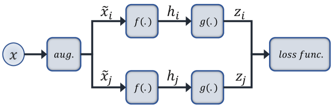
Figure 1: An overview of SimCLR.

The NT-Xent (normalized temperature-scaled cross-entropy) loss function introduced in [26] aims to maximize the similarity between positive pairs while minimizing the similarity between negative pairs. As a result, it has been widely used in the SimCLR setup (which we also use in our study). The loss function is defined as follows:

$$\mathcal{L}_{i,j}=-log(\frac{exp(sim(z_{i},z_{j})/\tau)}{\sum_{k=1}^{2N}\mathbbm{1}_{(k\neq i)}exp(sim(z_{i},z_{k})/\tau)}).$$ (1)

Here, for a batch of $N$ samples, by applying two augmentations per sample, the total data used for loss calculation becomes $2N$. The pairs $(z_{i},z_{j})$ are considered positive pairs, while they are considered negative pairs with respect to the remaining $2N-2$ samples. The temperature parameter $\tau$ serves to adjust the slope of the loss function. Specifically, higher values of $\tau$ result in a smoother loss function, while lower values yield a steeper loss function. The indicator function $\mathbbm{1}$ in the denominator of the equation takes a value of 1 when the samples are negative pairs, and 0 when they are positive pairs. The similarity function $sim$ employed in this analysis is the cosine similarity, defined as follows:

$$sim(z_{i},z_{j})=\frac{z_{i}.z_{j}}{\parallel z_{i}\parallel\parallel z_{j}\parallel}.$$ (2)

Upon training the model using the contrastive learning paradigm, the encoder model, $f(.)$, is used as a pre-trained feature extractor which could be used as frozen or fine-tuned for better domain alignment.

III-A2 BYOL

BYOL [27] (Bootstrap Your Own Latent) is an SSL technique that uses positive pairs to train deep neural networks. A visual representation of this method can be seen in Figure 2. This method involves the use of two networks, referred to as the online and target networks, which learn from each other by comparing the representation of an input sample as it passes through each network. Specifically, the online network is trained to recognize that the sample passing through the target network is the same as the original input sample. This interaction between the two networks allows for effective learning without the need for explicit labels.

In this method, a sample $x$ is first processed through an augmentation block, resulting in two different augmented versions, $\tilde{x_{i}}$ and $\tilde{x_{j}}$, which represent distinct perspectives of the same input sample. The first augmented version, $\tilde{x_{i}}$, is then passed through the online network encoder, denoted as $f_{\theta}(.)$, which produces a deeper representation $h_{i}$ of the sample. This representation is further processed through the online projection head, $g_{\theta}(.)$, to produce $z_{i}$. From the other side of the network, the second augmented version of the sample $x$, $\tilde{x_{j}}$, is passed through the target encoder, $f_{\zeta}(.)$, and projection head, $g_{\zeta}(.)$, to produce the representations $h_{j}$ and $z_{j}$, respectively.

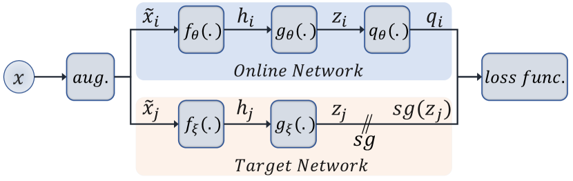
Figure 2: An overview of BYOL.

Since the online and target networks are both trained using different versions of the same sample, they are anticipated to contain similar information. The online network is trained to predict the target network representation, thus eliminating the need for negative pair training. This is achieved through the use of the function $q_{\theta}(.)$, which serves as a prediction mechanism for the online network to match the representations generated by the target network. The final representation of the online network, $z_{i}$, is passed through the predictor function $q_{\theta}(.)$, resulting in $q_{i}$. Meanwhile, a stop gradient (denoted as $sg$) is applied to the final representation of the target function, $z_{j}$, as only the weights of the online network will be updated at this stage. By learning to predict the representations generated by the target network, the online network encodes the underlying features of the input data effectively, leading to robust and highly representative feature extraction.

The loss function is designed to encourage the outputs of the online and target networks, represented by $q_{i}$ and $z_{j}$, to become more similar. This is achieved by calculating the mean squared error between the L2-normalized output of the online network’s predictor, and the final representation of the target network. The resulting loss is expressed in the following:

$$\mathcal{L}_{\theta,\zeta}=\|\bar{q_{i}}-\bar{z_{j}}\|^{2}_{2}=2-2.(\frac{\langle q_{i},z_{j}\rangle}{\|q_{i}\|_{2}.\|z_{j}\|_{2}}),$$ (3)

where $\bar{q_{i}},\bar{z_{j}}$ are the L2-normalized form of $q_{i},z_{j}$, and $\langle q_{i},z_{j}\rangle$ is the dot product of $q_{i},z_{j}$.

To ensure symmetry in the loss calculation, the input $\tilde{x_{i}}$ is fed to the target network, while $\tilde{x_{j}}$ is fed to the online network. The resulting loss, denoted as $\tilde{\mathcal{L}}_{\theta,\zeta}$, is computed. The final loss is given by $\mathcal{L}^{BYOL}_{\theta,\zeta}=\mathcal{L}_{\theta,\zeta}+\tilde{\mathcal{L}}_{\theta,\zeta}$, which combines the loss calculated from both the online and target networks and their flipped versions.

In each iteration of the training process, the target network’s weights are updated by taking a weighted average of the online network’s weights and the target network’s previous weights. The weight applied in this average, known as the exponential moving average decay, is predetermined and serves to gradually incorporate the weights of the online network into the target network, while maintaining some of the target network’s own previous weights to stabilize training.

One of the key benefits of BYOL is its use of SSL without the need for negative pairs. This reduces the difficulties associated with selecting negative pairs, such as the challenge of finding pairs that are appropriately challenging, as well as the problem of curriculum learning. The predictor function, $q_{\theta}(.)$, is specifically designed to learn to identify the semantic segments that are important for ECG signal classification, while ignoring irrelevant information, such as noise or errors in signal acquisition. This results in a model that is more robust to hyper-parameters and able to accurately classify ECG signals.

III-A3 SwAV

SwAV [28] (Swapping Assignment between Views) is an innovative clustering-based SSL approach that eliminates the need for pairwise comparisons, as briefly depicted in Figure 3. Unlike the two previous methods, the SwAV approach slightly changes the way the loss function and augmentation are implemented. This method starts by obtaining representations of the input data after undergoing various transformations. These representations are then assigned to codes using a cluster codebook and the Sinkhorn-Knopp algorithm [29]. The model compares the representations of each path with the codes assigned to the opposite path and attempts to minimize the loss function and bring the representations closer together. In the following paragraphs, we will provide a more in-depth explanation of the SwAV method.

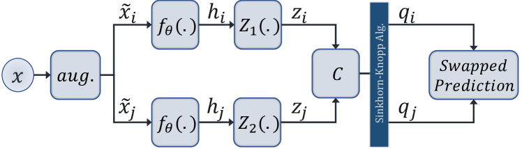
Figure 3: An overview of SwAV.

This method begins by applying augmentations to the ECG signal $x$ to obtain different views of the input signal, denoted as $\tilde{x_{i}}$ and $\tilde{x_{j}}$. These views are then processed through the network $f_{\theta}(.)$, resulting in representations $h_{i}$ and $h_{j}$. These representations are passed through shallow non-linear networks, $Z_{1}(.)$ and $Z_{2}(.)$, to produce $z_{i}$ and $z_{j}$. The next step involves utilizing a cluster codebook, or a set of prototypes, denoted as $C=[c_{1},c_{2},...,c_{K}]$, to assign representations to their corresponding codes. These prototype vectors are trained using the dominant features of the dataset. The prototype vectors can also be thought of as the weights of a single-layer fully connected network, where the dot product between the weights and the representations is calculated. The Sinkhorn-Knopp algorithm [29] is then applied to generate the codes for each sample, $q_{i}$ and $q_{j}$.

The next step in the process involves computing the loss for weight updates using the swapped prediction method. This involves utilizing the codes of sample $q_{i}$ to predict the representation of sample $z_{j}$, and vice versa. The loss is calculated by computing the cross entropy between the codes and the softmax of the dot product of the representations and cluster codes. This calculation enables the optimization of the weights, leading to improved predictions. The loss function for this process is given by the following equations:

$$\mathcal{L}_{z_{i},z_{j}}=l(z_{i},q_{j})+l(z_{j},q_{i}),$$ (4)

$$l(z_{a},q_{b})=-\sum_{k}{q_{b}^{k}\log\frac{exp(\frac{1}{\tau}z_{a}^{T}C_{k})}{\sum_{k^{{}^{\prime}}}{exp(\frac{1}{\tau}z_{a}^{T}{C_{k^{{}^{\prime}}}})}}},$$ (5)

where the temperature parameter, $\tau$, is used to regulate the confidence or uncertainty of the predictions. The higher the temperature value, the softer or more uncertain the output will be, and the lower the temperature value, the harder or more confident the output will be. Upon completion of training, the network $f_{\theta}(.)$ can be detached from the framework and be used as a powerful feature extractor for ECG signals or other types of data.

III-B Datasets

In this study, we aim to evaluate the performance of the aforementioned SSL methods in the context of ID and OOD data. To this end, we use several popular ECG-arrhythmia datasets, namely, PTB-XL [30], Chapman [31], and Ribeiro [32]. Below we provide the characteristics and details of these datasets.

PTB-XL. The PTB-XL [30] dataset is a publicly available resource and one of the largest of its kind for ECG signals. It serves as a widely used benchmark for evaluating the performance of models on 12-lead ECG signals, consisting of $18,885$ patient records, totalling $21,837$ records of $10$-second duration each, collected using Schiller AG devices between 1989 and 1996. The dataset is available at two different sampling frequencies: $100Hz$ and $500Hz$. In this study, we use the $100Hz$ version to limit the required computational resources. The PTB-XL dataset is comprised of three categories: Diagnostic, Form, and Rhythm, amounting to a total of 71 classes. In this study, we focus on the Diagnostic labelling category, which contains $5$ main categories. The dataset is relatively balanced in terms of gender, with $52\%$ male and $48\%$ female patients, and has a wide age range from $0$ to $95$ with a median of $62$ years.

Chapman. The Zhaoxing People’s Hospital and Chapman University have jointly collected and published a dataset in $2020$ that contains 12-lead ECG signals from $10,646$ patients [31]. The dataset includes ECG signals with both arrhythmia and various cardiovascular diseases, including $11$ rhythm conditions. The ECG signals are recorded with a duration of $10$ seconds at a sampling frequency of $500Hz$ and have undergone necessary pre-processing steps to ensure consistency with other datasets. This dataset is chosen for its size, comprehensiveness, and representation of various heart conditions. The age range of the participants in the dataset is from $4$ to $98$ years old, and it is relatively gender balanced with $44\%$ female and $56\%$ male participants. $17\%$ of the dataset consists of samples with a normal heartbeat, while the remaining $83\%$ have been diagnosed with a specific type of heart abnormality.

Ribeiro. The Telehealth Network of Minas Gerais in Brazil has compiled a dataset (Ribeiro [32]) of ECG signals for the purpose of evaluating the performance of algorithms for the diagnosis of cardiovascular abnormalities. The dataset includes $2,322,513$ samples from $1,676,384$ patients diagnosed with one of six specific abnormalities. The dataset is divided into training and test sets, with $98\%$ of the samples in the training set and the remaining $2\%$ in the test set, which amounts to approximately $50,000$ samples. The ages of the patients in the test set range from $16$ to over $81$ years old, and the dataset exhibits a bias towards female patients, with $39.7\%$ of the patients being male and the rest being female. The sampling frequency for this dataset is $400Hz$ which is pre-processed for the sake of consistency with other datasets. All of the conditions in the Ribeiro dataset can fall under the main category of Conduction Disturbance (CD), specifically, 1st-degree AV block (1dAVb), Right Bundle Branch Block (RBBB), Left Bundle Branch Block (LBBB), Sinus Bradycardia (SB), Atrial Fibrillation (AFIB).

III-C Implementation Details and Evaluation Protocol

The PTB-XL dataset is separated into ten subsections recommended by the original authors, based on which we create three primary sets for training, validation, and testing. Specifically, we use $8$ folds for training, $1$ fold for validation, and $1$ fold for testing. For the Chapman and Ribeiro datasets, we randomly select $80\%$ of the subjects for training, $10\%$ for validation, and the remaining $10\%$ for testing. This approach of dividing the datasets into three subsets helps ensure that the model is trained, validated, and tested on independent sets of data, which can provide accurate estimates of model performance with no leakage between the sets. Next, we down-sample the Chapman and Ribeiro datasets from $500Hz$ and $400Hz$ respectively to $100Hz$. The PTB-XL dataset is available in two versions, $100Hz$ and $400Hz$, and we opt for the former. Finally, as common in the area [23], we window the signals into $2.5$-second segments with no overlap, resulting in samples consisting of $250$ data points each.

During the pretraining phase, we optimize the NT-Xent loss which is described in section III-A. In this phase, the best model is selected based on the lowest loss observed on the validation set. In the fine-tuning phase, we use a binary cross-entropy loss and select the best model based on the highest F1-score observed on the validation set.

For training, we implement our method using PyTorch and utilize a pair of NVIDIA GeForce GTX 2080 GPUs. We adopt the Adam optimizer with a learning rate of $5\times 10^{-4}$ and weight decay of $1\times 10^{-3}$ to train the contrastive framework. For fine-tuning, we reduce the learning rate to $5\times 10^{-3}$ to prevent catastrophic forgetting and minimize the chance of overwriting the network weights completely. The contrastive stage is trained for $2000$ epochs with a batch size of $4096$ for SimCLR and BYOL, and a batch size of $1024$ for SwAV due to computational resource constraints. For the fine-tuning phase, we train the model for $50$ epochs.

We utilized the $xResNet1d50$ model as our backbone model for the experiments, as it was shown in [7] to achieve state-of-the-art results. This model is an adaptation of the well-known $ResNet50$ model for 1-dimensional data.

To evaluate performance, we use the macro F1-score instead of the micro F1-score. This is because the micro F1-score assigns equal weight to all observations, while the macro F1-score assigns equal weight to each class. Since most medical datasets, including ECG datasets, are imbalanced across classes, it is more reasonable to use a performance metric that treats all classes equally. Additionally, many medical datasets have more negative samples than positive ones. Therefore, metrics such as accuracy, which treats all samples equally, may not be suitable. By using the macro F1-score, we can accurately evaluate our model’s performance on imbalanced datasets while ensuring that each class is given equal weight.

III-D Augmentation Details

1) Gaussian Noise. We add a noise signal $N(t)$ to ECG signal $x(t)$. $N(t)$ is the same size as the ECG sample and each of its data points is driven from a Gaussian distribution with a mean equal to $0$, and a standard deviation equal to the adjustable parameter. We examined $\sigma_{G}=[0.01,0.1,1]$ in our experiments.

2) Channel Scaling. To obtain this augmentation, we multiply the ECG signal by a scaling factor $S$, which is a set of scaling factors for each of the 12 leads: $S=\{s_{i}\mid i=1,2,\dots,12\}$. Each $s_{i}$ is randomly derived from the range $[a,b]$, where both $a$ and $b$ are selected as augmentation parameters. We tested scaling factors in the range of $S_{ch}=[(0.33,3),(0.33,1),(0.5,2)]$ in our experiments.

3) Negation. The input signal is flipped vertically across the time axis as $\tilde{x}(t)=-x(t)$.

4) Baseline Wander. To simulate this type of noise in an ECG signal, we artificially introduce a low-frequency sinusoidal waveform with the frequency of $f_{w}$ to the original ECG signal. The sinusoidal waveform is generated with the chosen frequency, and the scale for the waveform is selected as $S_{bw}$. In our experiments, we choose the frequency of the sinusoidal $f_{w}=100$ and we test scales $S_{bw}=[0.1,0.7,1]$.

5) Electromyographic (EMG) Noise. To simulate EMG noise, high-frequency white Gaussian noise is used. This is because EMG noise is primarily caused by fast muscle contractions, which have high-frequency components [33]. A Gaussian distribution with a mean of $0$ is used, and the standard deviation of the distribution can be adjusted to achieve the desired level of noise. We use a variance equal to: $\sigma_{EMG}=[0.01,0.5,1]$ in our experiments.

6) Masking. This augmentation technique involves zeroing out specific segments of each lead in the ECG signal. To apply this technique, we first select the higher and lower bound of windows that we want to set to zero. Accordingly, two percentage values $a$ and $b$ are chosen as this augmentation’s parameters. Next, for each ECG signal in the batch, a random value $c$ is chosen from the range $[a,b]$, and using this value, a $c$% segment of that lead is set to zero. In our experiments we examined the following ranges for the masking parameters: $[10\%,20\%],[0\%,50\%],[40\%,50\%]$.

7) Time Warping. For this augmentation, we divide $x(t)$ into $w$ segments $x_{1}(t)$, $\cdots$, $x_{w}(t)$, where $w$ is the number of segments. Next, we use time warping to stretch half of the segments (randomly selected) by $r\%$ as the scaling factor, while simultaneously squeezing the other half by the same factor. The segments are finally concatenated in the same order to obtain $\tilde{x}(t)$ where the final length of $\tilde{x}(t)$ remains unchanged as $L$. We test the following list of parameters for this augmentation: $(w,r)=[(1,10),(3,5),(3,10)]$.

8) Combination of Augmentations. To further analyze the impact of augmentations on our pre-training process, we conduct additional experiments where we apply a combination of four augmentations simultaneously. This allows us to observe how different augmentations interact with each other and how this affects the performance of the models. In each iteration of pre-training, we randomly select four augmentations from our previously described list of augmentations. We select the parameters through experimentation with the goal of maximizing performance. The parameters for the augmentations when combined are as follows: Gaussian noise ($\sigma_{G}=1$), channel scaling ($S_{ch}=(0.33,3)$), baseline wander ($S_{bw}=1$), EMG noise ($\sigma_{EMG}=0.01$), masking ($[40\%,50\%]$), and time warping ($(w,r)=(1,10)$).

III-E Data Distribution

The distributions of data play a crucial role in this work as we aim to study a number of SSL techniques in ID and OOD settings. Therefore we analyze the three different datasets, namely Chapman, PTB-XL, and Ribeiro, in terms of data distributions to understand the relative relationships. To this end, we use a pre-trained model to process every sample $x^{D_{1}}_{i}$ from dataset $D_{1}$ and produce their respective outputs $y^{D_{1}}_{i}$ as illustrated in Figure 4. Similarly, samples $x^{D_{2}}_{i}$ from $D_{2}$ are passed through the same model to produce $y^{D_{2}}_{i}$. Dimensionality reduction is then applied on the resulting outputs ($y^{D_{1}}_{i}$ and $y^{D_{2}}_{i}$) using the UMAP method [34]. If the UMAP distributions of both datasets have overlaps, the samples from $D_{1}$ and $D_{2}$ can be considered ID. Conversely, if some parts of the UMAP distributions are not overlapped, they are considered OOD. As shown in Figure 4, the blue dots from $D_{1}$ are quite far from the orange dots from $D_{2}$, indicating that these two datasets are out-of-distribution with respect to each other.

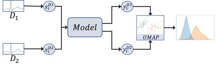
Figure 4: Data distribution analysis framework.

To mathematically measure the difference between the distributions of the two datasets, we use the approach presented in [35]. After obtaining the lower dimensional representations of $D_{1}$ and $D_{2}$ following UMAP ($\hat{y}^{D_{1}}_{i}$ and $\hat{y}^{D_{2}}_{i}$), we estimate their Probability Density Function (PDF)s. To quantify the degree of overlap between the two distributions, we calculate the overlapping index ($\eta$) using the following equation:

$$\eta(D_{1},D_{2})=\int_{-\infty}^{\infty}\min(f_{X}(x),f_{Y}(x))\mathrm{d}x$$ (6)

This formula computes the area under the curve where the PDFs overlap. If $\eta$ is close to one, the datasets are considered to be from similar distributions. However, if $\eta$ is significantly lower than one, it suggests that the datasets are out-of-distribution with respect to each other.

IV Results and Discussions

This section presents the results of our experiments and their implications. We begin by analyzing the distribution of the datasets used in this work, as described in Section III-E. Next, we evaluate the impact of different augmentation techniques on the performance of different SSL methods, as explained in Section III-D. This is followed by a comparison of the performance of the SSL methods themselves in the context of ID and OOD, as outlined in Section III-A. Finally, we examine how different factors influence the model’s ability to classify each disease class in the datasets.

IV-A Data Distribution Analysis

To demonstrate and analyze the distributions of the datasets used in this study, we use the training sets of the two larger datasets, PTB-XL and Chapman, for pre-training, while Ribeiro along with the test sets of PTB-XL and Chapman were used for testing. First, PTB-XL is used to train the xResNet1d50. backbone model, and the embeddings of the PTB-XL dataset (both train and test sets) are obtained. Next, dimensionality reduction is performed using UMAP, as shown in Figure 5 (left). Here we observe that the train and test sets of the PTB-XL dataset expectedly fall within the distributions of one another. In Figure 5 (right) we present the embeddings of the other two datasets (Chapman and Ribeiro) when a model that is pre-trained on PTB-XL (training set) is used to obtain the embeddings. It can be seen that the embeddings of Chapman and Ribeiro are considerably outside the distribution of PTB-XL, making our configuration of data effective for cross-dataset OOD analysis of ECG-based arrhythmia detection.

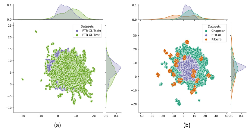
Figure 5: Visual representation of the distribution of the datasets. Part (a) illustrates the distributions of PTB-XL train and test subsets (ID) and part (b) shows the OOD instances (Chapman and Ribeiro) with respect to the PTB-XL dataset.

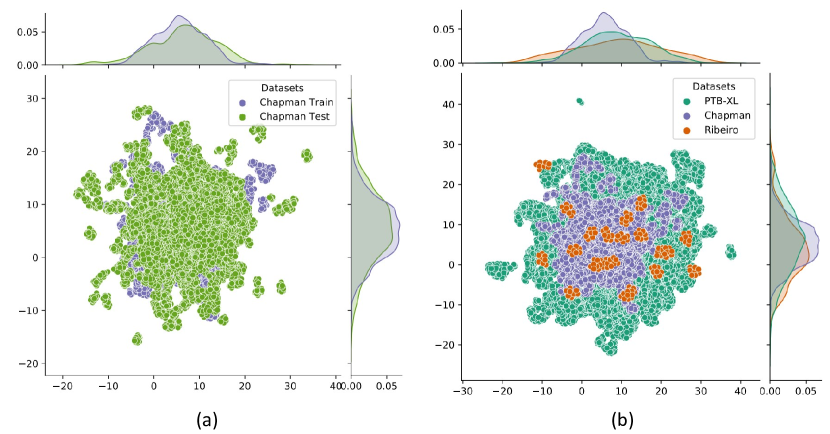
Figure 6: Visual representation of the distributions of the datasets used in our experiments. Part (a) illustrates the ID instances for the Chapman dataset, while part (b) shows the OOD instances (PTB-XL and Ribeiro) with respect to the Chapman dataset.

Here, we aim to quantify the distribution shifts using the procedure outlined in Section III-E. This procedure involves applying a Kernel Density Estimation (KDE) on the UMAP outputs to estimate PDFs for the distributions. The overlap between the train and test sets of the PTB-XL dataset is thus estimated by taking the integral of the overlapping area of the two KDEs. Our results, which are presented in Table I indicate that the overlap between the two distributions (PTB-XL train and test sets) is $83.52\%$. The same procedure is then applied to the Chapman and Ribeiro datasets, to calculate the overlap between the train set of the PTB-XL dataset and the other two datasets. The results show that the overlap between PTB-XL (train) and Chapman is $63.65\%$, and the overlap between PTB-XL (train) and Ribeiro is $46.36\%$. These results are depicted in Figure 7 and Table I. As per the results of this experiment, it can be concluded that the PTB-XL training and test sets are considered ID with each other while being considered OOD with Chapman and Ribeiro datasets.

TABLE I: Quantitative comparison of the distribution overlap between PTB-XL train and test sets (ID) and PTB-XL with Chapman and Ribeiro datasets (OOD).

Datasets	Overlap with PTB-XL Train Set
PTB-XL Test Set	$83.52\%$
Chapman	$63.65\%$
Ribeiro	$46.36\%$

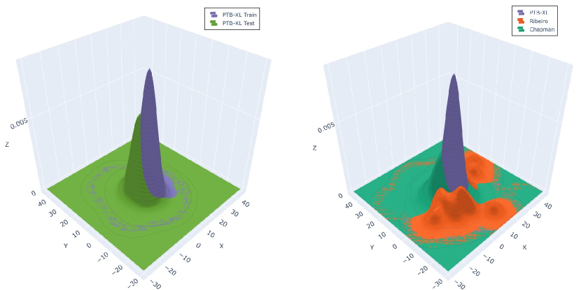
Figure 7: Comparing ID (PTB-XL train and test sets) against OOD (PTB-XL train set, Chapman, and Ribeiro) distribution overlaps through fitted KDE on the representations (left: ID, right: OOD).

Next, we repeat the same procedure using the Chapman dataset train and test set. Our results, which are shown in Table II, show that the overlap between the Chapman train and test sets is estimated as $82.52\%$. We also perform the procedure using the PTB-XL and the Ribeiro datasets to find the overlap with the Chapman train set. The overlap between the train set of the Chapman dataset and the PTB-XL dataset is calculated as $67.73\%$, while the overlap with the Ribeiro dataset is estimated to be $60.29\%$. These results are depicted in Figure 8. These results confirm that the PTB-XL and Ribeiro datasets can be considered OOD with respect to the Chapman train set, since their overlap is significantly lower than that of the Chapman train and test sets.

TABLE II: Quantitative comparison of the distribution overlap between Chapman train and test sets (ID) and Chapman with PTB-XL and Ribeiro datasets (OOD).

Datasets	Overlap with Chapman Train Set
Chapman Test Set	$82.52\%$
PTB-XL	$67.73\%$
Ribeiro	$60.29\%$

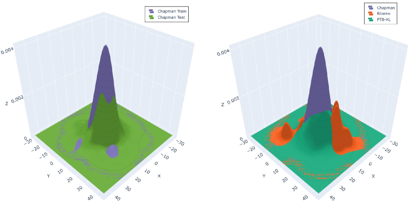
Figure 8: Comparing ID (Chapman train and test sets) against OOD (Chapman train set, PTB-XL, and Ribeiro) distribution overlaps through fitted KDE on the representations (left: ID, right: OOD).

TABLE III: Effect of combination of augmentations on SSL performance. The SSL methods are pre-trained on Chapman and PTB-XL, and tested on Chapman, PTB-XL, and Ribeiro datasets.

Method	Pretrained on	Tested on	F1-score
		PTB-XL	83.80
	PTB-XL	Chapman	67.68
SimCLR		Ribeiro	98.53
		PTB-XL	84.27
	Chapman	Chapman	67.16
		Ribeiro	98.52
		PTB-XL	82.84
	PTB-XL	Chapman	68.03
BYOL		Ribeiro	97.55
		PTB-XL	84.06
	Chapman	Chapman	69.74
		Ribeiro	98.30
		PTB-XL	84.80
	PTB-XL	Chapman	67.34
SwAV		Ribeiro	98.57
		PTB-XL	84.25
	Chapman	Chapman	70.89
		Ribeiro	99.00

IV-B SSL Method Performance

In this section, we conduct an extensive experiment to obtain a comprehensive evaluation on the performance of SSL methods for ECG-based arrhythmia detection. Based on the results from our data distribution analysis (Section IV-A) we use cross-dataset training and testing with Chapman and PTB-XL (train sets) used for training, while PTB-XL, Chapman, and Ribeiro datasets are used for testing. Our findings indicate that each of the SSL methods exhibit unique strengths and weaknesses, providing valuable insights into the performance of these approaches for ECG-based arrhythmia detection in ID and OOD settings.

Table IV presents the results, for the experiments conducted on the PTB-XL, Chapman, and Ribeiro datasets using each SSL method, as well as the results of training the models using a fully supervised model. As evident by the results, across all datasets, the performance of the SSL methods outperform that of fully supervised training. These findings suggest that SSL methods have significant potential for learning ECG representations and can be effectively leveraged for arrhythmia classification after finetuning.

Moreover, we observe that the SwAV method outperforms SimCLR and BYOL. For instance, when the model is pre-trained on Chapman and tested on the same dataset (ID), SwAV achieves an F1-score of $72.19\%$, which is higher than that of SimCLR ($71.95\%$) and BYOL ($70.69\%$) as shown in Table IV. Similarly, when the model is pre-trained on the PTB-XL dataset and tested on the Chapman dataset (OOD), SwAV achieves a higher F1-score ($70.47\%$) than SimCLR ($71.89\%$) and BYOL ($96.54\%$). Furthermore, when pre-trained on PTB-XL and tested on the same dataset (ID), SwAV achieves an F1-score of $85.43\%$, which is higher than SimCLR ($84.65\%$) and BYOL ($85.09\%$). Finally, when pre-trained on the Chapman dataset and tested on the PTB-XL dataset (OOD), SwAV achieves an F1-score of $85.53\%$, while SimCLR and BYOL achieve F1-scores of $84.38\%$ and $84.50\%$, respectively. Additionally, when pre-training the model using the Chapman dataset and testing on the Ribeiro dataset (OOD), the results show that SwAV obtains an F1-score of $99.10\%$, again outperforming SimCLR ($98.54\%$) and BYOL ($98.86\%$). When pre-training the models on the PTB-XL dataset and testing them on Ribeiro (OOD), SwAV obtains an F1-score of $97.97\%$ outperforming the other two methods, SimCLR ($97.93\%$) and BYOL ($97.39\%$). The results above confirm that SwAV is able to learn more effective representations for ECG-based arrhythmia detection, followed by SimCLR and BYOL. Prior work [23] has also shown the superiority of SimCLR over BYOL in the context of ECG learning.

TABLE IV: Comparison of best F1-scores for SimCLR, SwAV, and BYOL in arrhythmia classification from ECG signals on the PTB-XL, Chapman, and Ribeiro Datasets.

	SimCLR		BYOL		SwAV		Supervised
Pre-training	Chapman	PTB-XL	Chapman	PTB-XL	Chapman	PTB-XL
PTB-XL	$84.38\%$	$84.65\%$	$84.50\%$	$85.09\%$	85.53%	$85.43\%$	$80.24\%$
Chapman	$71.95\%$	$71.89\%$	$70.69\%$	$69.54\%$	72.19%	$70.47\%$	$70.96\%$
Ribeiro	$98.54\%$	$97.93\%$	$98.86\%$	$97.39\%$	99.10%	$97.97\%$	$84.84\%$

While Table IV presented the results using the ‘best’ settings, Table V demonstrates the results for the ‘average’ results (over various augmentations and respective parameters). Results again show that the SSL methods outperform the fully supervised model. These results also confirm that SwAV exhibits the best performance in terms of F1-scores among the three SSL methods. We hypothesize that the clustering-based approach in SwAV might have allowed the model to learn more robust and diverse representations that capture the essential and generalizable features of the ECG signals, leading to better performance. Clustering can be especially effective in cases where there are different underlying structures in the data, as it can help to identify this structure and improve the quality of the learned representations [36, 37, 38].

TABLE V: Comparison of average F1-scores for SimCLR, SwAV, and BYOL in arrhythmia classification from ECG signals on the PTB-XL, Chapman, and Ribeiro datasets.

	SimCLR		BYOL		SwAV		Supervised
Pre-training	Chapman	PTB-XL	Chapman	PTB-XL	Chapman	PTB-XL
PTB-XL	$83.44\%$	$83.54\%$	$83.11\%$	$82.91\%$	84.22%	$83.95\%$	$75.22\%$
Chapman	$66.99\%$	$65.69\%$	$67.15\%$	$65.36\%$	67.99%	$66.38\%$	$63.25\%$
Ribeiro	$96.40\%$	$95.13\%$	$96.89\%$	$94.12\%$	97.28%	$94.79\%$	$79.93\%$

TABLE VI: A comparison of the SSL results in comparison to a number of baselines tested on the PTB-XL dataset (on the left), and the Chapman dataset (on the right). The baseline results for the PTB-XL dataset have been reported in [7].

PTB-XL		Chapman
Method	AUC	Method	Ref.	AUC
LSTM	$92.7\%$	CPC	[39]	$84.4\%$
Inception1d	$93.1\%$	SSLECG	[9]	$52.6\%$
LSTM_bidir	$93.2\%$	CLOCS	[16]	$90.6\%$
Resnet1d_wang	$93.6\%$	w/o Inter	[12]	$76.4\%$
FCN_awng	$92.6\%$	w/o Intra	[12]	$92.1\%$
Wavelet+NN	$85.5\%$	ISL	[12]	$96.5\%$
xResnet1d101	$93.7\%$	SimCLR	-	$93.5\%$
Ensemble	$93.9\%$	BYOL	-	$94.9\%$
SimCLR	$93.6\%$	SwAV	-	96.7%
BYOL	$93.6\%$
SwAV	94.0%

In Table VI, we present a comparison between the SSL methods and popular models for the PTB-XL and the Chapman datasets. The models presented for the PTB-XL dataset are reported in [7], and for the Chapman dataset, the models are from the literature. To maintain consistency with other methods and for a fair comparison, we use the 4-class format of the Chapman dataset in this part of our study. For both of the datasets, the SwAV method shows the highest F1 among all the methods presented in the table.

As part of our methodology, we also conduct linear evaluations to assess the performance of the SSL models. This involves freezing the weights of the model after pre-training and adding a new fully connected layer. We then train this layer using labelled data without making any modifications to the pre-existing weights. The results are presented in Table VII. As expected, linear evaluation achieves lower scores than the fine-tuning approach (Table IV). However, linear evaluation still provides valuable insights into the effectiveness of the SSL models in ID and OOD settings. It allows us to measure the extent to which the models have learned useful and generalized representations during pre-training. The results (presented in Table VII) show that the model has performed reasonably well, even though the encoder is kept frozen, and this in turn shows that the model has learned meaningful and effective representations during the self-supervised pre-training.

Discussion. First, by comparing TablesIV and VII, we expectedly notice that fine-tuning the model on the target dataset will boost performance considerably for both ID and OOD schemes. However, we make an interesting and unexpected observation about the nature of ID and OOD ECG-based arrhythmia detection with SSL. By considering the results of Tables IV and VII, and comparing ID to OOD results within each table, we notice that in almost every scenario, the performance of the models are the same between OOD and ID setting. While this observation would be more expected with the fine-tuning setup, we even notice this trend with linear evaluation. This finding indicates that irrespective of dataset, equipment, and population of patients, SSL methods are able to effectively learn representations that can be used to accurately detect different types of arrhythmia. For instance, in the case of training SwAV on the Chapman dataset and testing on PTB-XL, despite the relatively OOD nature of these two datasets, we still witnessed comparable performance levels as when pre-training using the PTB-XL dataset and testing on the same dataset (see Table IV and Table VII for the reported results). This outcome suggests that the representations learned by SSL models can transfer effectively across diverse datasets and domains, regardless of the distribution shifts that may be present in the data, presenting important implications for practical applications.

TABLE VII: Linear evaluation on Chapman, PTB-XL and Ribeiro datasets.

	SimCLR		BYOL		SwAV
Pre-training	Chapman	PTB-XL	Chapman	PTB-XL	Chapman	PTB-XL
PTB-XL	$76.03\%$	$76.57\%$	$75.97\%$	$76.67\%$	79.61%	$79.60\%$
Chapman	$49.79\%$	$48.55\%$	$48.30\%$	$47.53\%$	50.37%	$49.85\%$
Ribeiro	$90.02\%$	$87.89\%$	$86.19\%$	$84.32\%$	93.37%	$86.96\%$

IV-C Per-Disease Analysis

Cardiovascular diseases encompass a wide range of conditions, some of which can be rare and life-threatening. In this section, we aim to evaluate the performance of SSL in the classification of each cardiovascular disease separately. To this end, we first present the per-class F1-scores of the best performing models for the PTB-XL dataset in Table VIII. Overall, the best performance of the models on the Normal class of the PTB-XL dataset is achieved when SwAV is pre-trained using the Chapman dataset, with an F1-score of $88.14\%$. The CD and MI classes also have relatively strong performances, with F1-scores of $80.85\%$ and $79.77\%$, respectively, when pre-trained on the PTB-XL dataset. However, identifying instances from the HYP and STTC classes prove more challenging for the models, with F1-scores of $71.96\%$ and $77.42\%$, respectively. This could indicate that features corresponding to some diseases are slightly more challenging to learn and detect compared to others.

Table VIII demonstrates that the SwAV model pre-trained on PTB-XL outperforms all other models in terms of F1-score for each class of the PTB-XL dataset, with the exception of the normal class, where pre-training on Chapman yields the best result.

TABLE VIII: Per-class results for the PTB-XL dataset.

	SimCLR		BYOL		SwAV
Pre-training	Chapman	PTB-XL	Chapman	PTB-XL	Chapman	PTB-XL
MI	$78.05\%$	$78.15\%$	$77.45\%$	$77.66\%$	$78.96\%$	79.77%
HYP	$67.82\%$	$67.34\%$	$66.08\%$	$64.44\%$	$70.07\%$	71.96%
Normal	$87.81\%$	$87.67\%$	$87.60\%$	$87.10\%$	88.14%	$88.06\%$
STTC	$75.78\%$	$75.22\%$	$74.33\%$	$74.59\%$	$76.62\%$	77.42%
CD	$79.41\%$	$80.15\%$	$79.42\%$	$79.59\%$	$80.84\%$	80.85%

To evaluate the performance of the models on the Chapman dataset, we use the 11-class configuration as described in Section III-B. Although the classes are not evenly distributed, we evaluate each class separately without making any adjustments to the dataset. The resulting per-class F1-scores are presented in Table IX.

TABLE IX: Per-class results for the Chapman dataset.

	SimCLR		BYOL		SwAV
Pre-training	Chapman	PTB-XL	Chapman	PTB-XL	Chapman	PTB-XL
AF	$55.58\%$	$56.59\%$	58.63%	$54.31\%$	$57.26\%$	$57.08\%$
AFIB	$90.37\%$	90.86%	$90.65\%$	$89.81\%$	$89.14\%$	$88.98\%$
AT	$9.09\%$	$8.99\%$	$6.74\%$	$6.90\%$	17.39%	$8.89\%$
AVNRT	$0.00\%$	$0.00\%$	$0.00\%$	$0.00\%$	$0.00\%$	$0.00\%$
AVRT	$0.00\%$	$0.00\%$	$0.00\%$	$0.00\%$	$0.00\%$	$0.00\%$
SI	31.49%	$29.94\%$	$26.87\%$	$30.81\%$	$29.67\%$	$30.32\%$
SAAWR	$0.00\%$	$0.00\%$	$0.00\%$	$0.00\%$	$0.00\%$	$0.00\%$
SB	$96.66\%$	$96.36\%$	96.72%	$96.56\%$	$96.45\%$	$96.35\%$
SR	$86.31\%$	96.09%	$86.34\%$	$95.91\%$	$86.22\%$	$85.67\%$
ST	$94.47\%$	$94.25\%$	$94.42\%$	$94.72\%$	94.92%	$94.51\%$
SVT	$85.68\%$	$84.22\%$	$85.64\%$	$85.29\%$	86.60%	$85.82\%$

The number of samples in each class of the Chapman dataset varies significantly, and there is a correlation between the number of samples and the model’s classification performance, as shown in Figure 9. SB disease is the most populated class, accounting for $36.53\%$ of the total samples, achieving the best result with an F1-score of $96.72\%$. The next most populated class is SR, accounting for $17.15\%$ of the total samples, and achieves an F1-score of $96.09\%$. For AFIB, ST, and SVT, the results are reasonable, but there is a drop in performance for classes with fewer samples. For instance, AF, which accounts for $4.18\%$ of the total samples, shows an F1-score of $58.63\%$, representing a $25\%$ drop from the previous class. SI and AT, which account for $3.75\%$ and $1.14\%$ of the dataset respectively, achieve F1-scores of $31.49\%$ and $17.39\%$. However, for AVNRT, AVRT, and SAAWR, which have less than $1\%$ distribution in the dataset, classification performances are poor.

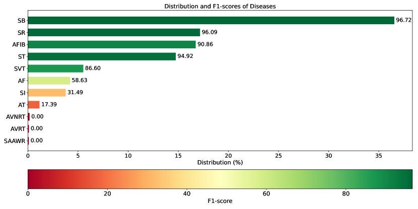
Figure 9: Chapman dataset classes distributions vs. F1-scores for each class.

Based on the analysis of the F1-scores presented in Table IX, it appears that pre-training the models on the Chapman dataset has yielded superior results for the majority of the disease classes compared to pre-training on the PTB-XL dataset, with the exception of AFIB and SR.

Finally, we present the F1-scores achieved for each disease class using the best performing model for the Ribeiro dataset in Table X. The results indicate that the BYOL method pre-trained on the Chapman dataset performs better than the other cases in classifying each disease class of the Ribeiro dataset, with the exception of the AFIB disease, where SimCLR pre-trained on the Chapman dataset achieved the best result. This may be due to the fact that the diseases in the Chapman dataset have more similarities to those in the Ribeiro dataset, as described in Section III-B. Specifically, the main class of all the diseases in the Ribeiro dataset belong to the CD category, which is well-represented in the Chapman dataset, but less so in PTB-XL. Considering the highest F1-scores in Table X, we can see that despite the low number of samples used for fine-tuning, all classes are classified well, except for However, the AFIB, which appears to be classified less accurately than the other classes.

TABLE X: Per-class results for the Ribeiro dataset.

	SimCLR		BYOL		SwAV
Pre-training	Chapman	PTB-XL	Chapman	PTB-XL	Chapman	PTB-XL
1-AVB	$93.33\%$	$81.08\%$	$83.33\%$	$82.35\%$	$93.88\%$	$95.24\%$
RBBB	$100.00\%$	$97.87\%$	$97.96\%$	$100.00\%$	$100.00\%$	$97.67\%$
LBBB	$100.00\%$	$100.00\%$	$100.00\%$	$100.00\%$	$100.00\%$	$100.00\%$
SBRAD	$100.00\%$	$100.00\%$	$100.00\%$	$100.00\%$	$95.24\%$	$100.00\%$
AFIB	$61.54\%$	$66.67\%$	$71.43\%$	$75.00\%$	$87.50\%$	$60.00\%$
STACH	$100.00\%$	$100.00\%$	$100.00\%$	$100.00\%$	$97.96\%$	$100.00\%$

V Conclusion and Future Work

In this paper we analyzed ECG-based arrhythmia detection using SSL methods, in ID and OOD settings. To this end, we studied the distributions of three popular ECG-based arrhythmia datasets to identify and quantify the their relative distributions and to determine whether they can be considered ID or OOD. Next, we implement three popular SSL methods, SimCLR, BYOL, and SwAV for ECG-based arrhythmia detection. In analyzing the augmentation parameters we found that in general, certain augmentation techniques such as mix of augmentations, time warping and masking, improve the learning of ECG representations and result in better generalization, while negation augmentation showed poor performance. In comparing different SSL techniques with state-of-the-art, we observed highly competitive performances in both ID and OOD settings, while among the SSL methods, SwAV outperformed the others. Another interesting finding of our work is that SSL techniques can detect arrhythmia in OOD settings with competitive performance to that of ID settings. Lastly, we conducted a per-class analysis for each dataset to understand the performance of the SSL methods toward detection of different diseases and found that false negative errors are more common than false positives.

A number of future directions can be considered to expand and improve upon the work presented in this paper. One approach in expanding our work could be to explore smaller step sizes and larger ranges of parameters for each augmentation in the search for the optimum augmentation parameters. Moreover, more advanced augmentations, for example those applied in the frequency domain, could be considered. In this study, we explored each augmentation individually, and the mix of all of the augmentations together. Nonetheless, different combinations of augmentations may exhibit various behaviors, which could be explored through forward/backward selection methodologies in the future. In terms of the SSL methods considered, more methods could be explored, and the number and type of architectures and backbone encoders could also be expanded. Lastly, using a combination of different datasets for pre-training the SSL models may result in learning more generalizable ECG representations, which could further improve the performance in OOD settings.

References

- [1] Johns Hopkins Medicine “Electrocardiogram”, Retrieved on January 13, 2023 from https://www.hopkinsmedicine.org/health/treatment-tests-and-therapies/electrocardiogram/, 2021
- [2] Ting Chen, Simon Kornblith, Mohammad Norouzi and Geoffrey Hinton “A simple framework for contrastive learning of visual representations” In International Conference on Machine Learning, 2020
- [3] Zhenzhong Lan et al. “Albert: A lite bert for self-supervised learning of language representations” In arXiv preprint arXiv:1909.11942, 2019
- [4] Jie Ren et al. “Likelihood ratios for out-of-distribution detection” In Advances in Neural Information Processing Systems, 2019
- [5] Weitang Liu, Xiaoyun Wang, John Owens and Yixuan Li “Energy-based out-of-distribution detection” In Advances in Neural Information Processing Systems, 2020
- [6] Kartik Ahuja et al. “Invariance principle meets information bottleneck for out-of-distribution generalization” In Advances in Neural Information Processing Systems, 2021
- [7] Nils Strodthoff, Patrick Wagner, Tobias Schaeffter and Wojciech Samek “Deep learning for ECG analysis: Benchmarks and insights from PTB-XL” In IEEE Journal of Biomedical and Health Informatics, 2020
- [8] Alexei Baevski, Yuhao Zhou, Abdelrahman Mohamed and Michael Auli “wav2vec 2.0: A framework for self-supervised learning of speech representations” In Advances in Neural Information Processing Systems, 2020
- [9] Pritam Sarkar and Ali Etemad “Self-supervised ECG representation learning for emotion recognition” In IEEE Transactions on Affective Computing, 2020
- [10] Pritam Sarkar and Ali Etemad “Self-supervised learning for ecg-based emotion recognition” In IEEE International Conference on Acoustics, Speech and Signal Processing, 2020
- [11] Pritam Sarkar et al. “Detection of maternal and fetal stress from the electrocardiogram with self-supervised representation learning” In Scientific Reports, 2021
- [12] Xiang Lan, Dianwen Ng, Shenda Hong and Mengling Feng “Intra-inter subject self-supervised learning for multivariate cardiac signals” In Proceedings of the AAAI Conference on Artificial Intelligence, 2022
- [13] Dani Kiyasseh, Tingting Zhu and David Clifton “CROCS: Clustering and retrieval of cardiac signals based on patient disease class, sex, and age” In Advances in Neural Information Processing Systems, 2021
- [14] Sahar Soltanieh, Ali Etemad and Javad Hashemi “Analysis of Augmentations for Contrastive ECG Representation Learning” In International Joint Conference on Neural Networks, 2022
- [15] Joseph Y Cheng et al. “Subject-aware contrastive learning for biosignals” In arXiv preprint arXiv:2007.04871, 2020
- [16] Dani Kiyasseh, Tingting Zhu and David A Clifton “Clocs: Contrastive learning of cardiac signals across space, time, and patients” In International Conference on Machine Learning, 2021
- [17] Jungwoo Oh et al. “Lead-agnostic self-supervised learning for local and global representations of electrocardiogram” In Conference on Health, Inference, and Learning, 2022
- [18] Bryan Gopal et al. “3KG: contrastive learning of 12-lead electrocardiograms using physiologically-inspired augmentations” In Machine Learning for Health, 2021
- [19] Hui Chen et al. “CLECG: A novel contrastive learning framework for electrocardiogram arrhythmia classification” In IEEE Signal Processing Letters, 2021
- [20] Dani Kiyasseh, Tingting Zhu and David Clifton “PCPs: Patient Cardiac Prototypes to Probe AI-based Medical Diagnoses, Distill Datasets, and Retrieve Patients” In Transactions on Machine Learning Research, 2023
- [21] Chuankai Luo et al. “Segment Origin Prediction: A Self-supervised Learning Method for Electrocardiogram Arrhythmia Classification” In International Conference of the IEEE Engineering in Medicine & Biology Society, 2021
- [22] Yuerong Zhou et al. “A contrastive learning approach for ICU false arrhythmia alarm reduction” In Scientific Reports, 2022
- [23] Temesgen Mehari and Nils Strodthoff “Self-supervised representation learning from 12-lead ECG data” In Computers in Biology and Medicine, 2022
- [24] Byeong Tak Lee, Seo Taek Kong, Youngjae Song and Yeha Lee “Self-Supervised Learning with Electrocardiogram Delineation for Arrhythmia Detection” In International Conference of the IEEE Engineering in Medicine & Biology Society, 2021
- [25] Huaicheng Zhang et al. “MaeFE: Masked Autoencoders Family of Electrocardiogram for Self-Supervised Pretraining and Transfer Learning” In IEEE Transactions on Instrumentation and Measurement, 2022
- [26] Kihyuk Sohn “Improved deep metric learning with multi-class n-pair loss objective” In Advances in Neural Information Processing Systems, 2016
- [27] Jean-Bastien Grill et al. “Bootstrap your own latent-a new approach to self-supervised learning” In Advances in Neural Information Processing Systems, 2020
- [28] Mathilde Caron et al. “Unsupervised learning of visual features by contrasting cluster assignments” In Advances in Neural Information Processing Systems, 2020
- [29] Marco Cuturi “Sinkhorn distances: Lightspeed computation of optimal transport” In Advances in Neural Information Processing Systems, 2013
- [30] Patrick Wagner et al. “PTB-XL, a large publicly available electrocardiography dataset” In Scientific Data, 2020
- [31] Jianwei Zheng et al. “A 12-lead electrocardiogram database for arrhythmia research covering more than 10,000 patients” In Scientific Data, 2020
- [32] Antônio H Ribeiro et al. “Automatic diagnosis of the 12-lead ECG using a deep neural network” In Nature Communications, 2020
- [33] Rahul Kher “Signal processing techniques for removing noise from ECG signals” In Biomedical Engineering and Research, 2019
- [34] Leland McInnes, John Healy and James Melville “Umap: Uniform manifold approximation and projection for dimension reduction” In arXiv preprint arXiv:1802.03426, 2018
- [35] Massimiliano Pastore and Antonio Calcagni “Measuring distribution similarities between samples: a distribution-free overlapping index” In Frontiers in Psychology, 2019
- [36] Anikó Vágner, László Farkas and István Juhász “Clustering and visualization of ECG signals” In Third International Conference on Software, Services and Semantic Technologies, 2011
- [37] Yun-Chi Yeh, Che Wun Chiou and Hong-Jhih Lin “Analyzing ECG for cardiac arrhythmia using cluster analysis” In Expert Systems with Applications, 2012
- [38] Hong He, Yonghong Tan and Jianfeng Xing “Unsupervised classification of 12-lead ECG signals using wavelet tensor decomposition and two-dimensional Gaussian spectral clustering” In Knowledge-Based Systems, 2019
- [39] William Falcon and Kyunghyun Cho “A framework for contrastive self-supervised learning and designing a new approach” In arXiv preprint arXiv:2009.00104, 2020