Critical transitions for scalar nonautonomous systems with concave nonlinearities: some rigorous estimates

Abstract.

The global dynamics of a nonautonomous Carathéodory scalar ordinary differential equation $x^{\prime}=f(t,x)$, given by a function $f$ which is concave in $x$, is determined by the existence or absence of an attractor-repeller pair of hyperbolic solutions. This property, here extended to a very general setting, is the key point to classify the dynamics of an equation which is a transition between two nonautonomous asypmtotic limiting equations, both with an attractor-repeller pair. The main focus of the paper is to get rigorous criteria guaranteeing tracking (i.e., connection between the attractors of the past and the future) or tipping (absence of connection) for the particular case of equations $x^{\prime}=f(t,x-\Gamma(t))$, where $\Gamma$ is asymptotically constant. Some computer simulations show the accuracy of the obtained estimates, which provide a powerful way to determine the occurrence of critical transitions without relying on a numerical approximation of the (always existing) locally pullback attractor.

1. Introduction

Tipping points, also called critical transitions, are sudden and large changes of a system’s dynamics as a consequence of small changes in its input. Under this headline, we find phenomena like disruption of climate [10, 23, 24], of ecological environments [35, 38], and of financial markets [32, 45], among others. From a mathematical standpoint, the understanding of certain critical transitions is still limited. Namely, when a time-dependent variation of parameters intervenes [21]. This is the case of rate-induced tipping [6, 7, 22, 30, 31, 42], size-induced tipping [30, 15], and phase-induced tipping [2, 3, 15, 30].

The setting of these problems is usually the same: an asymptotically constant time-dependent and known variation of a parameter takes place between a so-called past limit-problem (obtained as $t\to-\infty)$ and a future limit-problem (obtained as $t\to\infty)$; the past and the future limit-problems are also assumed to be known and at least a local attractor exists for each one of them. Depending on the nature of the time-dependent variation of parameters (e.g., its rate, phase and/or size) the “connection” between the attractors of the past and of the future can vary considerably or even break up. Every such qualitative change of dynamics is associated with a tipping point. Their analysis in asymptotically autonomous systems has been carried out with several mathematical techniques including compactification arguments [44, 43], statistical early-warning signals [39, 40], and the tipping probability of physical measures [5]. Numerous are also the instances of real models which have been studied, for example in climate [9], ecology [38, 42], and population dynamics [41].

Recently, an interpretation of these phenomena through nonautonomous bifurcation theory has arisen [30, 31]. In this new formulation, all the terms involved (the past and the future systems and the transition equations between them) are nonautonomous. There are two promising advantages in this new theory: on the one hand, this approach provides a unified framework for both asymptotically autonomous and nonautonomous systems; and, on the other hand, the assumptions required on the time-dependent variation of parameters, as well as the time-dependent forcing, are particularly mild compared to the rest of the literature. In the wake of such theory, this paper deals with the bifurcations occurring in coercive concave scalar nonautonomous ordinary differential equations. Although this class of problems might seem abstract, (globally or locally) concave or convex models are widely used in applied sciences [8, 11, 17, 37]. As an example and a motivation, we start our work in Section 2 by studying the occurrence of rate-induced and size-induced tipping in simple locally concave models from climate science and neural network theory.

The bulk of our results is theoretical, with potential relevance in the kind of problems mentioned above. We investigate families of scalar Carathéodory ordinary differential equations admitting bounded $m$-bounds and $l$-bounds, which allows the compactification of the equations in their hulls using a weak topology in the temporal variation of the vector fields. This type of coefficients and topologies are the natural language to formulate and solve control theory problems; for the same reasons, they are also appropriate for formulating and investigating problems related to critical transitions. In this paper, we show that, if one of these equations is concave, then the only possible bifurcation is the nonautonomous saddle-node bifurcation of a pair of hyperbolic solutions, and that all the tipping points occurring for these equations are in fact bifurcations of such type. This extends the previous conclusions obtained in [30, 31] for quadratic concave differential equations to this more general framework.

From here, we focus on transition equations of the form $x^{\prime}=f(t,x-\Gamma(t))$, where the asymptotic limits $\gamma_{\pm}$ of $\Gamma$ at $\pm\infty$ are well-defined and finite, and give rise to the past and future equations. To understand the geometry of the solutions of the transition equation is fundamental to achieve our main goal of obtaining calculable rigorous criteria which permit to identify some scenarios of tracking (with connection of attractors) and tipping (where the connection is lost). These criteria give a more trustworthy result as opposed to a finite numerical approximation of the locally pullback attractive solutions, which, by its own limited nature, can be wrong or misled. It is important to highlight that the inequalities that our criteria require are uncoupled: they depend on $\Gamma$ and on $x^{\prime}=f(t,x)$, but not on the transition equation itself.

Our criteria are obtained in two steps. In the first one, we deduce a set of inequalities providing tracking or tipping in the case of a piecewise constant transition function $\Gamma$. This kind of transitions have physical relevance and have been studied in some previous references in the literature [3, 19, 25]. For instance, they appear as limits of Carathéodory equations with continuous transitions, when some of the parameters decrease to $0$ or increase to infinity, providing a natural framework to study models with big or small size of physical parameters. Moreover, every continuous transition function $\Gamma$ can be well approximated by a suitable family of piecewise continuous functions. This property combined with the fact that some of the previously obtained inequalities hold uniformly for these piecewise continuous functions approximating $\Gamma$ allows us to obtain rigorous criteria for tracking or tipping also for continuous transition functions, which is the second step.

Let us delve with a bit more details into the main results. After the already mentioned Section 2, we present general results for coercive concave Carathéodory ordinary differential equations $x^{\prime}=f(t,x)$ in Section 3. Theorem 3.1 characterizes the sets of solutions bounded in the past and/or in the future, respectively bounded from above by a certain solution $a$ (defined at least on a negative half-line) and from below by a certain solution $r$ (defined at least on a positive half-line). Theorem 3.4 shows that $a$ and $r$ are globally defined and uniformly separated if and only if they are hyperbolic. This situation is referred to as the existence of an attractor-repeller pair $(a,r)$. The crucial property of persistence of hyperbolic solutions under small perturbations, a well-known property for more regular systems, is proved in Proposition 3.3 for the specific class of Carathéodory differential equations used in our work. Theorem 3.5 describes a nonautonomous global saddle-node bifurcation pattern, which is fundamental for the rest of the paper, and completes this section.

From this point, we consider a transition equation $x’=f(t,x-\Gamma(t))$, where $f$ is a concave and coercive Carathéodory function with smooth variation in the second component, and $\Gamma$ is an essentially bounded function with finite asymptotic limits $\gamma_{\pm}=\lim_{t\to\pm\infty}\Gamma(t)$. Our main hypothesis, also in force for the rest of the paper, is the existence of an attractor repeller pair $(a,r)$ for $x^{\prime}=f(t,x)$, which implies this same property for the past and future equations $x^{\prime}=f(t,x-\gamma_{\pm})$. In Section 4, we prove that the special solutions $a_{\Gamma}$ and $r_{\Gamma}$ provided by Theorem 3.1 have additional properties: $a_{\Gamma}$ is locally pullback attractive and connects with the attractor of the past as time decreases, and $r_{\Gamma}$ is locally pullback repulsive and connects with the repeller of the future as time increases. In addition, we classify in three cases the internal dynamics of the transition equation in terms of the domains and the relative position of both solutions. This classification combined with the previous bifurcation result shows that the collision of the attractor and the repeller is the unique mechanism leading to a critical transition for this type of equations.

For the rest of the paper, $\Gamma$ is also assumed to be continuous. A crucial role in our analysis will be played by some special maps: the concavity of $f$ ensures that, for any $\nu\in(0,1)$, the convex combination $b^{\nu}=\nu a+(1-\nu)r$ of the attractor $a$ and the repeller $r$ is a strict lower solution of $x^{\prime}=f(t,x)$. For each $h>0$, we define $\Gamma^{h}$ as the piecewise constant function which coincides with $\Gamma(t)$ at $t=jh$ for all $j\in\mathbb{Z}$. In Section 5, we analyze the transition equation $x’=f(t,x-\Gamma^{h}(t))$. Let us denote $a_{h}=a_{\Gamma^{h}}$ and $r_{h}=r_{\Gamma^{h}}$. The rigorous tracking and tipping criteria which we obtain in this section are based on the construction of a tracking route for the graph of $a_{h}$: the set $\mathcal{R}:=\bigcup_{m=1,\ldots n}\{(t,x)\,|\;t\in[(j_{0}+m-1)h,(j_{0}+m)h],\,x\geq b^{\nu_{m}}(t)+\Gamma((j_{0}+m)t)\}$. Theorem 5.4 provides suitable indices $j_{0},n\in\mathbb{Z}$, parameters $\nu_{1},\ldots,\nu_{m}\in[0,1]$ and a list of inequalities guaranteeing that the graph of $a_{h}$ remains in $\mathcal{R}$ for $t\in[j_{0}h,(j_{0}+n)h]$, and that $a_{h}((j_{0}+n)h)>r_{h}((j_{0}+n)h)$: this inequality ensures tracking. As pointed out before, the choice of the indices and parameters, and the inequalities to be satisfied, depend on $\Gamma$ and on the dynamics of $x^{\prime}=f(t,x)$, but not on that of $x^{\prime}=f(t,x-\Gamma(t))$. In the case of a nondecreasing $\Gamma$, Theorem 5.10 provides new lists of indices, parameters and inequalities (depending only on $\Gamma$ and on $x^{\prime}=f(t,x)$) which ensure that either $a_{h}$ blows up before $t=(j_{0}+n)h$ or its graph on $[j_{0}h,(j_{0}+n)h]$ is strictly below $\mathcal{R}$, with $a_{h}((j_{0}+n)h)<r_{h}((j_{0}+n)h)$: this inequality ensures tipping. Some easy applications of these results are also included in this section.

Section 6 deals with $x^{\prime}=f(t,x-\Gamma(t))$. Although the theory admits a general version, for the sake of simplicity we reduce the analysis to the quadratic function $f(t,x)=-x^{2}+p(t)$. Equations of this type are analyzed, for instance, in [6, 7, 39]. We point out that this transition equation can be rewritten as $x^{\prime}=-x(x-2\Gamma(t))+q(t)$ for $q=-\Gamma^{2}+p$: logistic nonautonomous models for population dynamics with migration term are included in our analysis. The unique (saddle-node) bifurcation value for $x^{\prime}=-(x-\Gamma(t))^{2}+p(t)+\lambda$ is the key point to provide rigorous conditions of tracking and total tracking on the hull of $p$; and, if $p$ is almost periodic, we describe simple situations with infinite tipping points caused by a phase shift on $p$. These are the main points of Theorem 6.2. Then, coming back to the main objective of the paper, we check that, for adequate choices of indices and parameters, the results obtained in the previous section remain uniformly valid for the piecewise transitions $\Gamma^{h}$ with $h>0$ small, and use this fact combined with the uniform convergence of $\Gamma^{h}$ to $\Gamma$ as $h\downarrow 0$ to provide rigorous criteria of tracking or tipping for the continuous transition. These criteria are given in Theorems 6.7, 6.8 and 6.9. Once more, the inequalities involved in the criteria depend only on $\Gamma$ and on $x^{\prime}=-x^{2}+p(t)$. Section 6 is completed with the particular case of a simple piecewise linear function $\Gamma$. We show that a simple application of the previous criteria allows us to distinguish the dynamical case of the transition equation in many cases, even for all the values of the rate and of the phase of the transition.

Some numerical examples intended to show the scope of our conclusions are included in Sections 5 and 6. In these examples, a big percentage of the cases of tracking or tipping satisfy some of the criteria of our theorems. To some extent, it seems correct to say that our sufficient conditions are a potent tool to determine the type of global dynamics in a high proportion of cases.

The paper ends with an Appendix on the compactification of the mild Carathéodory differential equation by means of the construction of the hull of $f$, and on the description of the main dynamical properties of the local skewproduct flow defined by the solutions of the equations given by the elements of the hull. These properties play an essential role in the development of the theory of this paper.

2. Examples of tipping in nonautonomous concave or convex models

Concave (or respectively convex) dynamics is the main focus of this paper. Although an assumption of concavity might seem strong, models which are at least locally concave (or convex) are greatly important and wide-spread in applications. As an example and a motivation for the subsequent theoretical analysis, we hereby include a short presentation of some locally concave or locally convex models which are susceptible to the tipping phenomena studied in the rest of the paper. The first example deals with three-parametric qualitative models of climate undergoing a rate-induced tipping, phase-induced and size-induced tipping. The second one shows a tipping point in a synchronized Hopfield neural network due to a change in the size of the one-parametric transition.

2.1. Tipping points for Fraedrich’s zero-dimensional climate models

In this section, we present three nonautonomous zero-dimensional models of the global climate obtained from the respective autonomous versions presented by Klaus Fraedrich in 1978 [17]. The underlying physical ground is given by an energy conservation law after integrating over the total mass (per unit area) of the system. Specifically, it is assumed that the average surface temperature $T(t)$ of a spherical planet subjected to radiative heating changes depending on the balance between incoming solar radiation $R\downarrow$ and outgoing emission $R\uparrow$:

$$\tau\,T^{\prime}=R\downarrow-R\uparrow.$$ (2.1)

The temperature is measured in Kelvin degrees and therefore the model is considered for $T>0$ (i.e., above the absolute zero), and the time is measured in seconds. The constant $\tau$ is the thermal inertia of a well-mixed ocean of depth 30 meters, covering 70.8% of the planet (see (2.5) for its value and those of the remaining constants). We model the incoming solar radiation by

$$R\!\downarrow\,=\frac{1}{4}\,\mu(t)\,I_{0}\,(1-\alpha)\,,$$

where $I_{0}$ is the average total solar irradiance at Earth and $\alpha$ is the albedo of the planet, i.e., the fraction of solar radiation which is reflected from the surface of Earth outside the atmosphere (for example due to ice, deserts or clouds). The positive function $\mu(t)$ allows for variations of the total solar irradiance. In contrast to Fraedrich, who takes $\mu=1$ for his first models, we consider a periodic coefficient $\mu(t)$ which simulates the following astronomical phenomena: the 11-year cycle of solar activity (also known as the Schwabe cycle) with amplitude $0.05\%$ of $I_{0}$, and the annual revolution of Earth along its elliptic orbit with amplitude $0.02\%$ of $I_{0}$ (see [20]). In other words, we consider

$$\mu(t)=1+0.0005\,\sin\!\left(\frac{2\pi t}{11\,\kappa}\right)+0.0002\,\sin\left(\frac{2\pi t}{\kappa}\right),$$ (2.2)

where $\kappa:=60{\cdot}60{\cdot}24{\cdot}365.25$ is the average number of seconds per year. Several other time-dependent components on time scales that vary from minutes till tens or hundreds of millennia could be included. We avoid it for at least two reasons: the most relevant time-scale for our subsequent tipping analysis is the one of decades; and our aim is to analyze the different causes for the occurrence of a tipping point in the asymptotically time-dependent case, not to provide a definitive quantitative estimate of the current or future climate on Earth.

The outgoing radiation $R\uparrow$ is modelled via the Stefan-Boltzmann law, i.e., proportional to a blackbody surface emission

$$R\!\uparrow\,=\varepsilon_{sa}\,\sigma\,T^{4}\,,$$

where $\varepsilon_{sa}=\varepsilon_{s}-\varepsilon_{a}$ stands for the effective emissivity obtained as the difference between the surface emissivity and the atmospheric emittance, and $\sigma$ is the Stefan–Boltzmann constant. With the previous definitions, (2.1) reads as the following zero-dimensional model for the planet’s average temperature,

$$T^{\prime}=\frac{1}{\tau}\,\left(-\varepsilon_{sa}\,\sigma\,T^{4}+\frac{1}{4}\,\mu(t)\,I_{0}\,(1-\alpha)\right).$$ (2.3)

A first refinement of this model is given by adding an albedo feedback law. Indeed, the albedo of a planet can be related to the average temperature via the amount of ice on the planet’s surface. Fraedrich [17] employs and motivates the use of a quadratic law $\alpha=a-b\,T^{2}$, which yields

$$T^{\prime}=\frac{1}{\tau}\,\left(-\varepsilon_{sa}\,\sigma\,T^{4}+\frac{1}{4}\,\mu(t)\,I_{0}\,b\,T^{2}+\frac{1}{4}\,\mu(t)\,I_{0}\,(1-a)\right)=:f_{1}(t,T)\,.$$ (2.4)

The equilibria, their hyperbolicity and the bifurcation points of the autonomous model (2.4) (with $\mu(t)\equiv 1$) have been studied in detail by Fraedrich [17], taking

$$\begin{split}&\tau:=10^{8}\,kg\,K^{-1}s^{-2}\,,\quad\varepsilon_{sa}:=0.62\,,\quad\sigma:=5.6704{\cdot}10^{-8}\,Wm^{-2}K^{-4}\,,\\ &I_{0}:=1366\,Wm^{-2}\,,\quad b:=10^{-5}K^{-2}\,,\quad a:=1.2\,.\end{split}$$ (2.5)

For these values, there are always (at least) two hyperbolic equilibria, one stable $T_{s}$ and the other unstable $T_{u}$, which form an attractor-repeller pair for $T>0$.

To simplify the notation in the next paragraphs, we call $I(t):=\mu(t)\,I_{0}$.

In what follows, we adapt an idea used by Ashwin et al. [7] (in the case $\mu(t)\equiv 1)$ to our nonautonomous setting: we substitute the parameters $a$ and $b$ by asymptotically autonomous functions of time, accounting for the anthropogenic emissions (combined greenhouse gasses and industrial aerosols) in the atmosphere; and we let $a$ vary with respect to a new parameter $d$. More precisely, once a function $b(t)>0$ is chosen, we take $a(t)=a_{d}(t):=1+d\,m(t)$ for $m(t):=I_{-}b^{2}(t)/(16\,\varepsilon_{sa}\,\sigma)$, with $I_{-}\leq I(t)$ for all $t\in\mathbb{R}$, and where $d$ varies in a range which we will specify later. Then, for each fixed time $s$, we rewrite (2.4) as the differential equations

$$T^{\prime}=\frac{1}{\tau}\,\left(-\varepsilon_{sa}\,\sigma\,T^{4}+\frac{1}{4}\,I(t)\,b(s)\,T^{2}-\frac{1}{4}\,I(t)\,d\,m(s)\right)=:g_{s}^{d}(t,T)\,.$$ (2.6)

The family $\{T^{\prime}=g_{s}^{d}(t,T)\,|\;s\in\mathbb{R}\}$ plays a fundamental role to analyze $T^{\prime}=g_{t}^{d}(t,T)$ (i.e., (2.6) with $s=t$): this last equation can be understood as a transition between the past and future equations, which are obtained by changing $b(s)$ and $m(s)$ by the values of their limits at $-\infty$ and $+\infty$, and which are nonautonomous due to $I(t)$. Note that analyzing the occurrence of critical transitions for $T^{\prime}=g_{c(t+l)}^{d}(t,T)$ as either $c$, $d$, or $l$ vary, we are analyzing the occurrence of either rate-induced, size-induced, or phase-induced critical points due to the transition $(b,a_{d})$.

A simple quantitative study of (2.6) gives immediate qualitative information on its possible dynamics. Below, we will find a constant $T_{1}$ such that $g_{s}^{d}(t,T)<0$ for all $t,s\in\mathbb{R}$ whenever $T<T_{1}$. Hence, any constant temperature $T<T_{1}$ is an upper solution for (2.6) for any $s\in\mathbb{R}$, which means that any solution starting below such threshold is destined to decrease as time increases. Furthermore, we will find a second constant $T_{2}<T_{1}$ such that, for all $t,s\in\mathbb{R}$, $g_{s}^{d}(t,T)$ is concave for $T>T_{2}$. In other words, in the region of the phase space where the dynamics is not already clear, the problem is concave and therefore can be completely investigated using the theory developed in the rest of the paper.

It is easy to check that, whenever $0<d<1$, the map $T\mapsto g_{s}^{d}(t,T)$ (a fourth-degree polynomial) has two different positive roots for each $(s,t)$, namely

$$T_{s}^{\pm}(t)=\left(\frac{b(s)\sqrt{I(t)}}{8\,\varepsilon_{sa}\,\sigma}\,\left(\sqrt{I(t)}\pm\sqrt{I(t)-d\,I_{-}}\right)\right)^{1/2}\,.$$

The temperatures $T_{1}$ and $T_{2}$ before described can be taken as

$$T_{1}:=\left(\frac{b_{+}I_{+}}{8\,\varepsilon_{sa}\,\sigma}\right)^{1/2}\qquad\text{and}\qquad T_{2}:=\left(\frac{b_{+}I_{+}}{24\,\varepsilon_{sa}\,\sigma}\right)^{1/2}\,,$$

where $I_{+}\geq I(t)$ for all $t\in\mathbb{R}$ and $b_{-}\leq b(s)\leq b_{+}$ for all $s\in\mathbb{R}$: $T_{1}$ satisfies $T_{1}\geq\sup_{t,s\in\mathbb{R}}T_{s}^{+}(t)$, and $\sup_{t,s\in\mathbb{R}}(\partial^{2}/\partial T^{2})\,g_{s}^{d}(t,T)<0$ for $T>T_{2}$.

Note that $\sup_{t\in\mathbb{R}}T_{s}^{-}(t)<\inf_{t\in\mathbb{R}}T_{s}^{+}(t)$ for each $s\in\mathbb{R}$ if $I_{+}-\sqrt{I_{+}\,I_{-}\,(1-d)}<I_{-}+I_{-}\sqrt{1-d}$ for $I_{+}\geq\sup_{t\in\mathbb{R}}I(t)$; i.e., if $0<d<d_{1}:=1-(\sqrt{I_{+}/I_{-}}-1)^{2}$. In this case, a strict lower solution exists for each equation (2.6)_s (including $s=\pm\infty$, i.e., the past and future equations), and it lies in the area of concavity whenever $T_{2}\leq\sup_{s,t\in\mathbb{R}}T_{s}^{-}(t)$, which we assume from now on (and which occurs if $d>5/9$). This existence ensures the occurrence of an attractor-repeller pair of solutions for (2.6)_s: a pair of hyperbolic solutions, attractive the upper one and repulsive the lower one, which determine the global dynamics in $\mathbb{R}\times(T_{2},\infty)$. Similarly, $\sup_{t,s\in\mathbb{R}}T_{s}^{-}(t)<\inf_{t,s\in\mathbb{R}}T_{s}^{+}(t)$ if $b_{+}\big{(}I_{+}-\sqrt{I_{+}\,I_{-}\,(1-d)}\big{)}<b_{-}\big{(}I_{-}+I_{-}\sqrt{1-d}\big{)}$ where $b_{-}\leq b(s)\leq b_{+}$ for all $s\in\mathbb{R}$; i.e., if $0<d<d_{2}:=1-\big{(}b_{+}I_{+}/(b_{-}I_{-})-1\big{)}^{2}\big{(}b_{+}\sqrt{I_{+}}/(b_{-}\sqrt{I_{-}})+1\big{)}^{-2}$ (which satisfies $d_{2}\leq d_{1}$). This property ensures that also the transition equation $T^{\prime}=g_{t}^{d}(t,T)$ has a strict lower solution in the area of concavity, and hence an atractor-repeller pair. In addition, using similar techniques to those of [30, 31], it can be proved that this attractor-repeller pair approaches that of the past equation as time decreases and that of the future equation as time increases, which is the situation usually called tracking. And this is true for all the equations $T^{\prime}=g_{c(t+l)}^{d}(t,T)$ for $c>0$ and $l\in\mathbb{R}$. In other words: there are no critical transitions of rate-induced, size-induced or phase-induced type for $d\in(5/9,d_{2})$.

It can also be proved that, if $d\in(5/9,d_{1})$, the existence of an attractor-repeller pair for $T^{\prime}=g_{s}^{d}(t,T)$ for each $s\in\mathbb{R}$ ensures the absence of critical transitions for a rate $c>0$ small enough. We will now construct an example showing that, for a fixed $d\in(d_{2},d_{1})$, rate-induced tipping may occur as $c$ increases, and that the value of the critical point may change with the initial phase. And will also show that size-induced tipping may occur for a fixed small rate for values of $d$ slightly greater than $d_{1}$. We take the same $b(t)$ as in [7], namely

$$b(t):=1.690{\cdot}10^{-5}(1-\lambda(t/\kappa))+1.835{\cdot}10^{-5}\lambda(t/\kappa)$$

where $\lambda(t)=ke^{t}/(1+ke^{t})$ satisfies $\lambda(0)=10^{-6}$. Recall that $I(t):=\mu(t)\,I_{0}$ for $\mu$ given by (2.2), and that $m(t):=I_{-}b^{2}(t)/(16\,\varepsilon_{sa}\,\sigma)$. We consider the three-parametric family of equations

$$T^{\prime}=\frac{\kappa}{\tau}\,\left(-\varepsilon_{sa}\,\sigma\,T^{4}+\frac{1}{4}\,I(\kappa\,u)\,b(c\kappa(u+l))\,T^{2}-\frac{1}{4}\,I(\kappa\,u)\,d\,m(c\kappa(u+l))\right)$$ (2.7)

where $u$ is time in years, $T(u)$ is the temperature in Kelvin and, for the transition: $c$ is the rate, $d$ determines its size, and $l$ is its initial phase. Taking $\mu_{-}:=0.99993$, $\mu_{+}:=1.00007$, $b_{-}=1.690{\cdot}10^{-5}$ and $b_{+}:=1.835{\cdot}10^{-5}$, we get $d_{1}=0.9999995097$, $d_{2}=0.9982486778$, $T_{1}=298.6397736$ and $T_{2}=172.4197537$. The numerical evidence, depicted in Figure 1, suggests that any tipping point for this model happens through the collision of an attractor and a repeller which do no longer exist after the critical transition. This is in fact the only mechanism leading to a tipping point in “the concave region” of this model, as we shall see in Section 3.

Figure 1. Different critical transitions occur for (2.7) depending on the values of $d$, $l$ and $c$. In the horizontal axes, time in years; in the vertical ones, temperature in Kelvin. The solid red and dashed blue lines are respectively the locally pullback attractive and locally pullback repulsive solutions. Tracking (or tipping) occurs whenever the red curve is above (or below) the blue one at a common value of the time. The first row shows that, for a fixed value of $d\in(d_{1},d_{2})$ and for $l=0$, a tipping rate $c$ occurs between $0.05$ and $0.07$; and a zoom shows the (always present) oscillatory character of the solutions. The first two panels in the second row provide a more accurate approximation for the critical rate, while the third and forth ones show that a different initial phase in the transition ($l=20$) means a different value for the critical rate. The third row shows the occurrence of a size-induced critical transition as $d$ increases for fixed values of $c$ and $l$.

Fraedrich [17] presents two additional models with a greenhouse feedback law (respectively derived from (2.3) and (2.4)). The underlaying motivation is that the temperature and the amount of vapour water in the air depend on each other. An empirical relation between the temperature and the long-wave radiation $L\!\uparrow$ of the atmosphere is the so-called Swinbank’s formula according to which $L\!\uparrow\,\sim T^{6}$. Therefore, it is assumed that $\varepsilon_{a}$ follows a quadratic law, $\varepsilon_{a}=\varepsilon_{c}+k\,T^{2}$, where $\varepsilon_{c}=0.0235\,\textrm{ln}(CO_{2})$ (with $CO_{2}$ in ppm) is the $CO_{2}$ emittance, and $k=3{\cdot}10^{-6}K^{-2}$ [17]. The basic climate model (2.3) with the greenhouse feedback law becomes

$$T^{\prime}=\frac{1}{\tau}\left(k\,\sigma\,T^{6}-\varepsilon_{sc}\,\sigma\,T^{4}+\frac{1}{4}\,\mu(t)\,I_{0}\,(1-\alpha)\right)=:f_{2}(t,T)\,,$$ (2.8)

with $\alpha=0.284$, $\varepsilon_{sc}=\varepsilon_{s}-\varepsilon_{c}=0.87$, and the rest of the constants as in (2.5). Finally, (2.3) with both the ice-albedo feedback and the greenhouse feedback laws becomes

$$T^{\prime}=\frac{1}{\tau}\left(k\,\sigma\,T^{6}-\varepsilon_{sc}\,\sigma\,T^{4}+\frac{1}{4}\,\mu(t)\,I_{0}\,b\,T^{2}+\frac{1}{4}\,\mu(t)\,I_{0}\,(1-a)\right)=:f_{3}(t,T)\,.$$ (2.9)

It is easy to check that $f_{2}(t,T)$ and $f_{3}(t,T)$ are convex in $T$ for all $t$ if $T$ is larger than a certain constant. Numerical simulations show that (2.8) and (2.9) also have an attractor-repeller pair in both their autonomous (with $\mu(t)\equiv 1$) and nonautonomous (with $\mu(t)$ given by (2.2)) versions. Importantly, this implies that a similar mechanism for tipping as the one in (2.4), due to the collision of the attractor and the repeller, is possible also in (2.8) and (2.9). However, the relative position of the attractor and repeller (and hence the whole dynamics) is inverted in the convex case with respect to that in the concave one. Hence, tipping points appearing in (2.8) and (2.9) are opposite in nature with respect to those in (2.4). Specifically, the concave problems passing through a bifurcation point will end up in a deep-frozen state, while the convex ones in an arid-desert state. It is worth noting that such a tipping point for the later models would take place at an earth temperature which is already beyond the survival of life on Earth, as we know it.

2.2. Critical transitions for Hopfield synchronized neural networks

A biological neuron is an electrically charged cell which is able to receive and transmit a signal via a complex electrochemical mechanism. In either case, each neuron has an equilibrium voltage where it tends to spontaneously remain in the absence of inputs. An inhibitory or excitatory signal pulse triggers a resistor-capacitor type exponential response followed by relaxation. Specifically, when the injected current causes the voltage to exceed a certain threshold $\Theta$, a special electrochemical process generates a rapid increase in the potential leading to a single non-weakening and propagating pulse. This phenomenon is called neuron firing. The pulse halts at the synapses where the transmission of the information to the next neurons is taken care of by special neurotransmitter molecules. Depending on the physiological effect that these neurotransmitter induces in the next neuron, the synapse is termed excitatory or inhibitory, whether they facilitate or not the occurrence of a pulse by increasing or lowering the potential of the next neuron.

An artificial neural network mimics the same process either using electrical components or as a software simulation on a digital computer. For this reason, the construction of a differential model of a neural network of $N$ neurons of either type can be carried out analogously. We follow the presentation by Wu [46], to which we point the interested reader for further details. We consider a network of $N>0$ neurons and denote by $x_{i}$, for $i=1,\dots,N$, the potential of the $i$-th neuron in terms of deviation from the equilibrium potential. The variable $x_{i}$ is also called the action potential or short-term memory or STM. The change of neuron potential can be caused by internal and external processes,

$$x_{i}^{\prime}=\left(x_{i}^{\prime}\right)_{\text{internal}}+\left(\left(x_{i}^{\prime}\right)_{\text{excitatory}}+\left(x_{i}^{\prime}\right)_{\text{inhibitory}}+\left(x_{i}^{\prime}\right)_{\text{stimuli}}\right)_{\text{external}}\,.$$

For the internal dynamics, it is assumed that, in absence of external inputs, the neurons’ potential decays exponentially to the equilibrium; i.e., for $i=1,\dots,N$,

$$\left(x_{i}^{\prime}\right)_{\text{internal}}=-a_{i}(t)\,x_{i}\quad\text{for some }a_{i}\colon\mathbb{R}\to(0,\infty)\,.$$

For the sake of simplicity, we assume that the external processes can be only excitatory or external stimuli (i.e., $(x_{i}^{\prime})_{\text{inhibitory}}\equiv 0$), following the laws

$$\left(x_{i}^{\prime}\right)_{\text{excitatory}}=\!\sum_{\begin{subarray}{c}k=1\\ k\neq i\end{subarray}}^{N}Z_{ik}(t)\,\widetilde{f}_{k}(x_{k}-\Theta_{k})\,,\qquad\left(x_{i}^{\prime}\right)_{\text{stim.}}=\widetilde{I}_{i}(t)\,,$$

where $\widetilde{f}_{k}:\mathbb{R}\to[0,\infty)$ is the signal function of the $k$-th neuron, $\Theta_{k}$ is the firing threshold, $Z_{ik}(t)=Z_{ki}(t)>0$ (also called the long-term memory or LTM) represents the synaptic coupling coefficient, and $\widetilde{I}_{i}(t)$ is the input from a contiguous patch of neurons. The signal function $\widetilde{f}_{k}$ is typically a step function, a piecewise linear function, or a sigmoid limiting at $0$ as $y\to-\infty$ and at $1$ as $y\to\infty$. In order to read the model as a classical Hopfield-type neural network (see [46, Chapter 4]), two steps are needed. First, we assume that the signal function $\widetilde{f}_{k}$ is a common increasing sigmoid $\widetilde{f}\colon\mathbb{R}\to[0,1]$ for all the neurons, and define $f(x)=2\,\widetilde{f}(x)-1$, which is strictly increasing and limits at $\pm 1$ as $y\to\pm\infty$. That is, we obtain

$$x_{i}^{\prime}=-a_{i}(t)\,x_{i}+\frac{1}{2}\,\sum_{\begin{subarray}{c}k=1\\ k\neq i\end{subarray}}^{N}Z_{ik}(t)\,f(x_{k}-\Theta_{k})+\widetilde{I}_{i}(t)+\frac{1}{2}\,\sum_{\begin{subarray}{c}k=1\\ k\neq i\end{subarray}}^{N}Z_{ik}(t)\,.$$

Second, we make the changes of variables $y_{i}=x_{i}-\Theta_{i}$, so that $y_{i}$ measures the deviation of the voltage of the $i-th$ neuron from its activation threshold, getting

$$y_{i}^{\prime}=-a_{i}(t)\,y_{i}+\frac{1}{2}\,\sum_{\begin{subarray}{c}k=1\\ k\neq i\end{subarray}}^{N}Z_{ik}(t)\,f(y_{k})+\widetilde{I}_{i}(t)+\frac{1}{2}\,\sum_{\begin{subarray}{c}k=1\\ k\neq i\end{subarray}}^{N}Z_{ik}(t)-\Theta_{i}\,a_{i}(t)\,.$$

Now, in order to get a synchronized neural network, we assume that $Z_{ik}(t)$ synchronize at a certain bounded continuous function $\widetilde{z}\colon\mathbb{R}\to(0,\infty)$ which can be fed into the previous equation as a reference trajectory. And we also assume that $a_{i}=a$, $\Theta_{i}=\Theta$, and $\widetilde{I}_{i}=\widetilde{I}$ for $i=1,\ldots,N$. So, whenever the system is initialized with synchronized (i.e., equal) initial conditions $y_{i}(0)=y_{0}$ for $i=1,\dots,N$, the resulting solutions remain synchronized for all $t>0$. In this case, the previous system reduces to a unique scalar differential equation satisfied by all the neurons,

$$y^{\prime}=-a(t)\,y_{i}+z(t)\,f(y)+I(t)\,,$$ (2.10)

where $z(t):=(N-1)\,\widetilde{z}(t)/2$ and $I(t):=\widetilde{I}(t)+(N-1)\,\widetilde{z}(t)/2-\Theta\,a(t)$. The function $a$ will be important for our tipping analysis, as better explained in what follows.

In our presentation, we will assume that $z(t)$ is positive and bounded, that $f(0)=0$, and that the resulting input $I(t)$ is mildly inhibitory: upper-bounded by a small negative constant $k<0$. Since, for $y>0$, $-a(t)\,y+z(t)\,f(y)+I(t)<f(y)\left\|z\right\|_{\infty}+k$, there is a value $\bar{y}>0$ such that, for all $y\in(0,\bar{y})$, the right-hand side of (2.10) is negative. In other words, every $y\in(0,\bar{y})$ is an upper solution for (2.10), which means that any solution starting below $\bar{y}$ is destined to decrease as time increases while it is positive. Hence, if a bounded and positive solution exists, then it is located above $\bar{y}$.

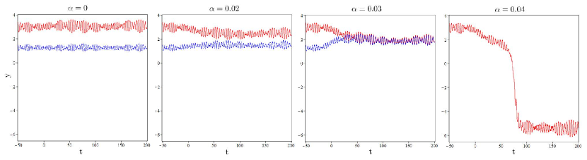
Figure 2. A time-dependent tipping scenario is depicted for the Hopfield-type differential equation (2.10) with $I(t)$ and $z(t)$ given by (2.12), and with $a(t)=a_{\alpha}(t)$ given by (2.11) and hence depending on the parameter $\alpha$ which characterizes the internal decay rate of a neuron: this rate increases with $\alpha$. After tipping (when the dashed blue line is no longer below the solid red one: see Figure 1), the set of synchronized neurons collapses to a (stable) “inactive” state. Indeed, after some time, the potential of each neuron remains uniformly bounded below the activation threshold 0.

For our tipping analysis, we assume that the internal decay rate $a(t)$ has a baseline behaviour $a_{0}(t)$ and an increasing trend with time (for example due to ageing): $a(t)$ becomes

$$\begin{split}a_{\alpha}(t)&:=a_{0}(t)+\alpha\,(1+e^{-t/5})^{-1}\\ &:=0.2\,\left(1+\sin(\pi t)\,\sin\big{(}((1+\sqrt{5})\,t)/2\big{)}\right)+\alpha\,(1+e^{-t/5})^{-1}\,.\end{split}$$ (2.11)

In addition, we take

$$\begin{split}f(y)&:=(1-e^{-y})/(1+e^{-y})\,,\\ I(t)&:=0.2\,\big{(}\sin(2\pi t/\sqrt{5})\,\cos(t/7)-1.5\big{)}\,,\\ z(t)&:=1+0.75\,\sin(t/7)\sin\big{(}(1+\sqrt{5})\,t/2\big{)}\,.\end{split}$$ (2.12)

Note that the function $-a(t)\,y_{i}+z(t)\,f(y)+I(t)$ is concave in $y$ for $y>0$ and convex for $y<0$, since so is $f$ and $z(t)\geq 0.25$.

As shown in Figure 2, there exists a value $\alpha>0$ beyond which the set of synchronized neurons collapses to a (stable) “inactive” state: some time after $t=0$ the state of each neuron remains uniformly bounded below the activation threshold (which is 0 after the change of variables). Observe finally that the critical transition occurs as $\alpha$ increases. Since $\alpha$ determines the size of the transition, we have a size-induced tipping point.

3. General results for concave and coercive Carathéodory ODEs

Throughout the paper, $L^{\infty}=L^{\infty}(\mathbb{R},\mathbb{R})$ is the Banach space of essentially bounded functions $q\colon\mathbb{R}\to\mathbb{R}$ endowed with the norm $\left\|q\right\|_{L^{\infty}}$ given by the inferior of the set of real numbers $k\geq 0$ such that of $l(\{\,t\in\mathbb{R}\>|\;|q(t)|>k\,\})=0$, where $l(\mathcal{I})$ is the Lebesgue measure of $\mathcal{I}\subseteq\mathcal{R}$. We write “ $l$-a.a.” instead of “for Lebesgue almost all $t\in\mathbb{R}$”, “Lebesgue almost always” and “Lebesgue almost all”.

We consider nonautonomous scalar equations of the type

$$x^{\prime}=f(t,x)\,,$$ (3.1)

where $f:\mathbb{R}^{2}\to\mathbb{R}$ is assumed to satisfy (all or part of) the next conditions:

• $f$ is Borel measurable;

• for all $j\in\mathbb{N}$ there exists $m^{f}_{j}\in\mathbb{R}$ such that, $l$-a.a., $\sup_{x\in[-j,j]}|f(t,x)|\leq m^{f}_{j}$.

• for all $j\in\mathbb{N}$ there exists $l^{f}_{j}\in\mathbb{R}$ such that, $l$-a.a., $\sup_{x_{1},\,x_{2}\in[-j,j]}|f(t,x_{2})-f(t,x_{1})|/|x_{2}-x_{1}|\leq l^{f}_{j}$;

• $l$-a.a., the map $x\mapsto f(t,x)$ is $C^{1}$;

• the map $x\mapsto f_{x}(t,x)$ satisfies condition f3, where $f_{x}=\partial f/\partial x$;

• (coercivity) there exists a subset $\mathcal{R}\subseteq\mathbb{R}$ with full Lebesgue measure and $\delta>0$ such that $\limsup_{x\to\pm\infty}f(t,x)/x^{2}<-\delta$ uniformly on $\mathcal{R}$;

• (strict concavity) for all $j\in\mathbb{N}$ there exists a constant $\delta_{j}>0$ such that, $l$-a.a., $\sup_{x_{1},\,x_{2}\in[-j,j],\,x_{1}\neq x_{2}}(f_{x}(t,x_{2})-f_{x}(t,x_{1}))/(x_{2}-x_{1})<-\delta_{j}$.

All these conditions are in force unless otherwise stated. The results establishing the existence, uniqueness and properties of maximal solutions of (3.1) for $f$ satisfying f1, f2 and f3 (less restrictive conditions, in fact) can be found in [13, Chapter 2]. In the usual terminology for Carathéodory and Lipschitz-Carathéodory equations, conditions f2 and f3 mean the existence of $L^{\infty}$ $m$-bounds and $l$-bounds, respectively. It is easy to check that, if $f$ satisfies f1 and f3, then it is strong Carathéodory: the map $x\mapsto f(t,x)$ is continuous on $\mathbb{R}$ for $l$-a.a. $t\in\mathbb{R}$. Conditions f4 and f5 require more regularity on the state variable $x$, and will allow us to discuss hyperbolicity of solutions of (3.1). Note that, if f4 holds, condition f3 ensures f2 for $f_{x}$. Conditions f6 and f7 provide us with a framework where, for instance, the existence of an attractor-repeller pair of hyperbolic solutions can be discussed.

Let $t\mapsto x(t,s,x_{0})$ denote the maximal solution of (3.1) satisfying $x(s,s,x_{0})=x_{0}$, defined on $\mathcal{I}_{s,x_{0}}=(\alpha_{s,x_{0}},\beta_{s,x_{0}})$ with $-\infty\leq\alpha_{s,x_{0}}<s<\beta_{s,x_{0}}\leq\infty$. Recall that, in this setting, a solution is an absolutely continuous function on each compact interval of $\mathcal{I}_{s,x_{0}}$ which satisfies (3.1) at Lebesgue a.a. $t\in\mathcal{I}_{s,x_{0}}$; and that $\mathcal{I}_{s,x_{0}}=\mathbb{R}$ if $x(t,s,x_{0})$ is bounded. The results establishing the existence, uniqueness and properties of this maximal solution for $f$ satisfying f1, f2 and f3 (less restrictive conditions, in fact) can be found in [13, Chapter 2]. Recall also that the real map $x$, which is defined on an open subset of $\mathbb{R}\times\mathbb{R}\times\mathbb{R}$ containing $\{(s,s,x_{0})\,|\;s,x_{0}\in\mathbb{R}\}$, satisfies $x(s,s,x_{0})=x_{0}$ and $x(t,l,x(l,s,x_{0}))=x(t,s,x_{0})$ whenever all the involved terms are defined. In addition, since the countable intersection of subsets of $\mathbb{R}$ with full Lebesgue measure has full Lebesgue measure, property f7 ensures that, for $l$-a.a. $t\in\mathbb{R}$, the map $x\mapsto f_{x}(t,x)$ is strictly decreasing, and hence $f(t,(1-\rho)x_{1}+\rho x_{2})>(1-\rho)f(t,x_{1})+\rho f(t,x_{2})$ for all $x_{1},x_{2}\in\mathbb{R}$ and $\rho\in(0,1)$. In turn, this last property guarantees the strict concavity of $x_{0}\mapsto x(t,s,x_{0})$ for fixed $t>s$: the statements and proof of  [30, Proposition 2.3] are also valid in the more general setting here considered.

3.1. The special solutions $\mathfrak{a}$ and $\mathfrak{r}$

The coercivity property f6 has consequences on the properties of the sets

$$\begin{split}\mathcal{B}^{-}&:=\Big{\{}(s,x_{0})\in\mathbb{R}^{2}\,\Big{|}\;\sup_{t\in(\alpha_{s,x_{0}},s]}x(t,s,x_{0})<\infty\Big{\}}\,,\\ \mathcal{B}^{+}&:=\Big{\{}(s,x_{0})\in\mathbb{R}^{2}\,\Big{|}\;\inf_{t\in[s,\beta_{s,x_{0}})}x(t,s,x_{0})>-\infty\Big{\}}\,,\\ \end{split}$$

which may be empty. We fix any $\varepsilon>0$ and take $m>0$ large enough to satisfy $f(t,x)\leq-\varepsilon$ for all $t\in\mathcal{R}$, and $|x|\geq m$. By rewriting as $x(t)=x(s)+\int_{s}^{t}f(l,x(l))\,dl$, it is easy to check that any solution remains upper bounded as time increases and lower bounded as time decreases, with $\limsup_{t\to(\beta_{s,x_{0}})^{-}}x(t)<m$ and $\liminf_{t\to(\alpha_{s,x_{0}})^{+}}x(t)>-m$. We will often use these properties in the paper without further reference. They imply that $\mathcal{B}^{-}$ (resp. $\mathcal{B}^{+}$) is the set of pairs $(s,x_{0})$ giving rise to solutions which remain bounded in the past (resp. in the future). Note that $\alpha_{s,x_{0}}=-\infty$ for all $(s,x_{0})\in\mathcal{B}^{-}$ and $\beta_{s,x_{0}}=\infty$ for all $(s,x_{0})\in\mathcal{B}^{+}$. The set $\mathcal{B}:=\mathcal{B}^{-}\cap\mathcal{B}^{+}$ is the (possibly empty) set of pairs $(s,x_{0})$ giving rise to (globally defined) bounded solutions of (3.1).

The next result is proved by repeating the arguments leading to [30, Theorem 2.5] (in turn based on [31, Theorem 3.1]). Conditions f4, f5 and f7 are not required.

Theorem 3.1.

Let $\mathcal{B}^{\pm},\mathcal{B}$ and $m$ be the sets and constant above defined.

• If $\mathcal{B}^{-}$ is nonempty, then there exist a set $\mathcal{R}^{-}$ coinciding with $\mathbb{R}$ or with a negative open half-line and a maximal solution $a\colon\mathcal{R}^{-}\to(-\infty,m)$ of (3.1) such that, if $s\in\mathcal{R}^{-}$, then $x(t,s,x_{0})$ remains bounded as $t\to-\infty$ if and only if $x_{0}\leq a(s)$; and if $\sup\mathcal{R}^{-}<\infty$, then $\lim_{t\to(\sup\mathcal{R}^{-})^{-}}a(t)=-\infty$.

• If $\mathcal{B}^{+}$ is nonempty, then there exist a set $\mathcal{R}^{+}$ coinciding with $\mathbb{R}$ or with a positive open half-line and a maximal solution $r\colon\mathcal{R}^{+}\to(-m,\infty)$ of (3.1) such that, if $s\in\mathcal{R}^{+}$, then $x(t,s,x_{0})$ remains bounded as $t\to+\infty$ if and only if $x_{0}\geq r(s)$; and if $\inf\mathcal{R}^{+}>-\infty$, then $\lim_{t\to(\inf\mathcal{R}^{+})^{+}}r(t)=\infty$.

• Let $x$ be a solution defined on a maximal interval $(\alpha,\beta)$. If it satisfies $\liminf_{t\to\beta^{-}}x(t)=-\infty$, then $\beta<\infty$; and if $\limsup_{t\to\alpha^{+}}x(t)=\infty$, then $\alpha>-\infty$. In particular, any globally defined solution is bounded.

• The set $\mathcal{B}$ is nonempty if and only if $\mathcal{R}^{-}=\mathbb{R}$ or $\mathcal{R}^{+}=\mathbb{R}$, in which case both equalities hold, $a$ and $r$ are globally defined and bounded solutions of (3.1), and $\mathcal{B}=\{(s,x_{0})\in\mathbb{R}^{2}\,|\;r(s)\leq x_{0}\leq a(s)\}\subset\mathbb{R}\times[-m,m]$.

• Let the function $b\colon\mathbb{R}\to\mathbb{R}$ be bounded, continuous, of bounded variation and with nonincreasing singular part on every compact interval of $\mathbb{R}$. Assume that $b^{\prime}(t)\leq f\big{(}t,b(t)\big{)}$ for $l$-a.a. $t\in\mathbb{R}$. Then, $\mathcal{B}$ is nonempty, and $r\leq b\leq a$. If, in addition, there exists $t_{0}\in\mathbb{R}$ such that $b^{\prime}(t_{0})<f\big{(}t_{0},b(t_{0})\big{)}$, then $r<a$. And, if $b^{\prime}(t)<f\big{(}t,b(t)\big{)}$ for $l$-a.a. $t\in\mathbb{R}$, then $r<b<a$.

Remark 3.2.

As explained in [30, Remark 2.6], (3.1) has a bounded solution if and only if there exists a time $t_{0}$ such that the solutions $a$ and $r$ defined in Theorem 3.1 are respectively defined at least on $(-\infty,t_{0}]$ and $[t_{0},\infty)$, with $a(t_{0})\geq r(t_{0})$; and the inequality $a(t_{0})>r(t_{0})$ is equivalent to the existence of at least two bounded solutions. If $t_{0}$ with $a(t_{0})<r(t_{0})$ exists, then there are no bounded solutions.

3.2. Hyperbolic solutions, their persistence, and local pullback attractor and repellers

In this subsection, conditions f6 and f7 are not required. A bounded solution $\widetilde{b}\colon\mathbb{R}\to\mathbb{R}$ of (3.1) is said to be hyperbolic if the corresponding variational equation $z^{\prime}=f_{x}(t,\widetilde{b}(t))\,z$ has an exponential dichotomy on $\mathbb{R}$. That is (see [14]), if there exist $k\geq 1$ and $\beta>0$ such that either

$$\exp\int_{s}^{t}f_{x}(l,\widetilde{b}(l))\,dl\leq k\,e^{-\beta(t-s)}\quad\text{whenever $t\geq s$}$$ (3.2)

or

$$\exp\int_{s}^{t}f_{x}(l,\widetilde{b}(l))\,dl\leq k\,e^{\beta(t-s)}\quad\text{whenever $t\leq s$}$$ (3.3)

holds. In the case (3.2), the hyperbolic solution $\widetilde{b}$ is said to be (locally) attractive, and in the case (3.3), $\widetilde{b}$ is (locally) repulsive. In both cases, we call $(k,\beta)$ a (non-unique) dichotomy constant pair for the hyperbolic solution $\widetilde{b}$, or for the linear equation $z^{\prime}=f_{x}(t,\widetilde{b}(t))\,z$.

Condition f5 shows the existence of the Lipschitz coefficient $l^{f_{x}}=l^{f_{x}}(\rho)$ appearing in the statement of the next result.

Proposition 3.3.

Assume the existence of an attractive (resp. repulsive) hyperbolic solution $\widetilde{b}_{f}$ of $x^{\prime}=f(t,x)$ with dichotomy constant pair $(k_{f},\beta_{f})$. Take $\rho>0$ and a constant $l^{f_{x}}\geq\sup_{x_{1},x_{2}\in[-\rho,\rho],x_{1}\neq x_{2}}|f_{x}(t,\widetilde{b}_{f}(t)+x_{1})-f_{x}(t,\widetilde{b}_{f}(t)+x_{2})|/|x_{1}-x_{2}|\,$ $l$-a.a. Then, given $\beta\in(0,\beta_{f})$, there exists $\delta^{*}=\delta^{*}(k_{f},\beta,\rho,l^{f_{x}})>0$ such that, for any $\delta_{*}\in(0,\delta^{*}]$, the equation $x^{\prime}=g(t,x)$ has an attractive (resp. repulsive) hyperbolic solution $\widetilde{b}_{g}$ with $\big{\|}\widetilde{b}_{f}-\widetilde{b}_{g}\big{\|}_{\infty}\leq\delta_{*}$ and dichotomy constant pair $(k_{f},\beta)$ provided that

• $g$ satisfies f1, f2, f3, f4 and f5,

• $\big{|}g(t,\widetilde{b}_{f}(t))-f(t,\widetilde{b}_{f}(t))\big{|}\leq\beta\,\delta_{*}/(2k_{f})$ $l$-a.a.,

• $\sup_{x\in[-\rho,\rho]}|f_{x}(t,\widetilde{b}_{f}(t)+x)-g_{x}(t,\widetilde{b}_{f}(t)+x)|<\beta_{f}-\beta$ $l$-a.a.,

• $\sup_{x_{1},x_{2}\in[-\rho,\rho],x_{1}\neq x_{2}}|g_{x}(t,\widetilde{b}_{f}(t)+x_{2})-g_{x}(t,\widetilde{b}_{f}(t)+x_{1})|/|x_{2}-x_{1}|\leq l^{f_{x}}$ $l$-a.a.

Proof.

The proof, similar to that of [31, Proposition 3.2], is based on [1, Lemma 3.3]. We include the details in this Carathéodory setting for the reader’s convenience.

Let us work in the attractive case. We call $\mathcal{B}_{\nu}:=\{\bar{y}\in C(\mathbb{R},\mathbb{R})\,|\;\left\|\bar{y}\right\|_{\infty}\leq\nu\}$ for $\nu>0$ and, to simplify the notation, $b:=\widetilde{b}_{f}$. We assume that $g$ satisfies conditions 1, 3 and 4, and call $l^{f,g}_{\rho}:=\beta_{f}-\beta-\sup_{|x|\leq\rho}|f_{x}(t,\widetilde{b}_{f}(t)+x)-g_{x}(t,\widetilde{b}_{f}(t)+x)|$. Condition f5 allows us to find $\delta\in(0,\rho]$ such that $|f_{x}(t,b(t)+\bar{y}(t))-f_{x}(t,b(t))|\leq l^{f,g}_{\rho}$ $\,l$-a.a. if $\bar{y}\in\mathcal{B}_{\delta}$, and hence, using hypothesis 3,

$$\begin{split}g_{x}(t,b(t)+\bar{y}(t))&=f_{x}(t,b(t)+\bar{y}(t))+(g_{x}(t,b(t)+\bar{y}(t))-f_{x}(t,b(t)+\bar{y}(t)))\\ &\leq f_{x}(t,b(t))+(\beta_{f}-\beta)\end{split}$$

$l$-a.a. This bound combined with relation (3.2) for $b$ ensures that, if $\bar{y}\in\mathcal{B}_{\delta}$, then

$$\exp\int_{s}^{t}g_{x}(l,b(l)+\bar{y}(l))\,ds\leq k_{f}\,e^{-\beta(t-s)}\quad\text{whenever $t\geq s$}\,.$$ (3.4)

In particular, if $\widetilde{b}_{g}=b+\bar{y}$ is a solution of $x^{\prime}=g(t,x)$, then it is hyperbolic attractive with dichotomy pair $(k_{f},\beta)$ and satisfies $\big{\|}\widetilde{b}_{g}-b\big{\|}_{\infty}=\left\|\bar{y}\right\|_{\infty}\leq\delta$. Our goal is hence to look for such a function $\bar{y}$, which will be obtained as the unique fixed point of a contractive operator $T\colon\mathcal{B}_{\delta_{*}}\to\mathcal{B}_{\delta_{*}}$ if $\delta_{*}\in(0,\delta^{*}]$ for a suitable $\delta^{*}\in(0,\delta]$.

Let us define $T$. The change of variable $y=x-b(t)$ takes $x^{\prime}=g(t,x)$ to

$$y^{\prime}=g_{x}(t,b(t))\,y+h(t,y)\,,$$

where $h(t,y):=g(t,b(t))-f(t,b(t))+r(t,y)$ for $r(t,y):=g(t,b(t)+y)-g(t,b(t))-g_{x}(t,b(t))\,y$. Relation (3.4) for $\bar{y}=0$ ensures that

$$u(t,s):=\exp\int_{s}^{t}g_{x}(l,b(l))\,dl\leq k_{f}e^{-\beta(t-s)}\quad\text{whenever $t\geq s$}\,.$$

Clearly, $t\mapsto u(t,s)$ solves $y^{\prime}=g_{x}(t,b(t))\,y$ with $u(s,s)=0$. It is easy to check (see [14, Section 3]) that, for each $\bar{y}\in\mathcal{B}_{\delta}$,

$$T\bar{y}(t):=\int_{-\infty}^{t}u(t,s)\,h(s,\bar{y}(s))\,ds$$

is the unique bounded solution of $y^{\prime}=g_{x}(t,b(t))\,y+h(t,\bar{y}(t))$, and that

$$\begin{split}\left\|T\bar{y}\right\|_{\infty}&\leq\left\|h(\cdot,\bar{y}(\cdot))\right\|_{L^{\infty}}k_{f}/\beta\,,\\ \left\|T\bar{y}_{1}-T\bar{y}_{2}\right\|_{\infty}&\leq\left\|r(\cdot,\bar{y}_{1}(\cdot))-r(\cdot,\bar{y}_{2}(\cdot))\right\|_{L^{\infty}}k_{f}/\beta\,.\end{split}$$ (3.5)

Let us fix $\delta^{*}\in(0,\delta]$ such that $l^{f_{x}}\delta^{*}<0.9\,\beta/k_{f}$, take any $\delta_{*}\in(0,\delta^{*}]$, and assume that $g$ also satisfies 2. To check that $T\colon\mathcal{B}_{\delta_{*}}\to\mathcal{B}_{\delta_{*}}$ is well-defined, it suffices to check that $|h(t,\bar{y}(t))|\leq\beta\,\delta_{*}/k_{f}$ $l$-a.a. if $\bar{y}\in\mathcal{B}_{\delta_{*}}$, and this bound follows from $\big{|}g(t,b(t))-f(t,b(t))\big{|}\leq\beta\,\delta_{*}/(2k_{f})$ $l$-a.a. (according to hypothesis 2) and $|r(t,\bar{y}(t))|\leq l^{f_{x}}|\bar{y}(t)|^{2}/2\leq l^{f_{x}}(\delta_{*})^{2}/2<\beta\,\delta_{*}/(2k_{f})$ $l$-a.a. (by Taylor’s theorem, hypothesis 4 and the choice of $\delta^{*}$). Similarly, $|r(t,\bar{y}_{1}(t))-r(t,\bar{y}_{2}(t))|\leq l^{f_{x}}|\bar{y}_{1}(t)-\bar{y}_{2}(t)|^{2}/2\leq l^{f_{x}}\delta_{*}|\bar{y}_{1}(t)-\bar{y}_{2}(t)|\leq(0.9\,\beta/k_{f})\,|\bar{y}_{1}(t)-\bar{y}_{2}(t)|$ $l$-a.a. if $\bar{y}_{1},\,\bar{y}_{2}\in\mathcal{B}_{\delta_{*}}$, which combined with the second bound in (3.5) shows that $T\colon\mathcal{B}_{\delta_{*}}\to\mathcal{B}_{\delta_{*}}$ is contractive. We represent its unique fixed point by $\bar{y}_{g}\in\mathcal{B}_{\delta_{*}}$. Then $\widetilde{b}_{g}:=\widetilde{b}_{f}+\bar{y}_{g}$ solves $x^{\prime}=g(t,x)$. As said before, this completes the proof. ∎

Let us define local pullback attractors and repellers, which may appear also in the absence of hyperbolic solutions, and which will play a fundamental role in the dynamical description of the next sections. A solution $\bar{a}\colon(-\infty,\beta)\to\mathbb{R}$ (with $\beta\leq\infty$) of (3.1) is locally pullback attractive if there exist $s_{0}<\beta$ and $\delta>0$ such that, if $s\leq s_{0}$ then the solutions $x(t,s,a(s)\pm\delta)$ are defined on $[s,s_{0}]$ and, in addition,

$$\lim_{s\to-\infty}|\bar{a}(t)-x(t,s,\bar{a}(s)\pm\delta)|=0\quad\text{for all $t\leq s_{0}$}\,.$$

A solution $\bar{r}\colon(\alpha,\infty)\to\mathbb{R}$ (with $\alpha\geq-\infty$) of (3.1) is locally pullback repulsive if the solution $\bar{r}^{*}\colon(-\infty,-\alpha)\to\mathbb{R}$ of $y^{\prime}=-h(-t,y)$ given by $\bar{r}^{*}(t)=\bar{r}(-t)$ is locally pullback attractive. That is, if there exist $s_{0}>\alpha$ and $\delta>0$ such that, if $s\geq s_{0}$, then the solutions $x(t,s,\bar{r}(s)\pm\delta)$ are defined on $[s_{0},s]$ and, in addition,

$$\lim_{s\to\infty}|\bar{r}(t)-x(t,s,\bar{r}(s)\pm\delta)|=0\quad\text{for all $t\geq s_{0}$}\,.$$

3.3. Occurrence of an attractor-repeller pair

The main results in this paper rely on the fact that if the considered equation has a local attractor, such attractor is in fact part of a classical attractor-repeller pair of hyperbolic solutions. Theorem 3.4 (proved in Appendix A) shows that the solutions $a$ and $r$ associated to (3.1) by Theorem 3.1 are globally defined and uniformly separated if and only if they are hyperbolic, in which case they provide the mentioned attractor-repeller pair. The global dynamics in the case of existence of such a pair is jointly described by Theorems 3.1 and 3.4.

Recall that conditions f1-f7 are assumed on $f$, unless otherwise indicated.

Theorem 3.4.

Assume that (3.1) has bounded solutions, and let $a$ and $r$ be the (globally defined) functions provided by Theorem 3.1. Then, the following assertions are equivalent:

• The solutions $a$ and $r$ are uniformly separated: $\inf_{t\in\mathbb{R}}(a(t)-r(t))>0$.

• The solutions $a$ and $r$ are hyperbolic, with $a$ attractive and $r$ repulsive.

• The equation (3.1) has two different hyperbolic solutions.

In this case,

• let $(k_{a},\beta_{a})$ and $(k_{r},\beta_{r})$ be dichotomy constant pairs for the hyperbolic solutions $a$ and $r$, respectively, and let us choose any $\bar{\beta}_{a}\in(0,\beta_{a})$ and any $\bar{\beta}_{r}\in(0,\beta_{r})$. Then, given $\varepsilon>0$, there exist $k_{a,\varepsilon}\geq 1$ and $k_{r,\varepsilon}\geq 1$ (respectively depending also on the choices of $\bar{\beta}_{a}$ and of $\bar{\beta}_{r}$) such that

  $$\begin{split}&\quad\qquad|a(t)-x(t,s,x_{0})|\leq k_{a,\varepsilon}\,e^{-\bar{\beta}_{a}(t-s)}|a(s)-x_{0}|\quad\text{if $x_{0}\geq r(s)+\varepsilon$ and $t\geq s$}\,,\\ &\quad\qquad|r(t)-x(t,s,x_{0})|\leq k_{r,\varepsilon}\,e^{\bar{\beta}_{r}(t-s)}|r(s)-x_{0}|\quad\text{if $x_{0}\leq a(s)-\varepsilon$ and $t\leq s$}\,.\end{split}$$

  In addition,

  $$\begin{split}&\quad\qquad|a(t)-x(t,s,x_{0})|\leq k_{a}\,e^{-\beta_{a}(t-s)}|a(s)-x_{0}|\quad\text{if $x_{0}\geq a(s)$ and $t\geq s$}\,,\\ &\quad\qquad|r(t)-x(t,s,x_{0})|\leq k_{r}\,e^{\beta_{r}(t-s)}|r(s)-x_{0}|\quad\text{if $x_{0}\leq r(s)$ and $t\leq s$}\,.\end{split}$$

• The equation (3.1) has no more hyperbolic solutions, and $a$ and $r$ are the unique bounded solutions of (3.1) which are uniformly separated.

3.4. A nonautonomous saddle-node bifurcation pattern.

Let us take $f$ as in (3.1) (i.e., satisfying f1-f7), and consider the parametric perturbations

$$x^{\prime}=f(t,x)+\lambda\,.$$ (3.6)

Let $\mathcal{B}_{\lambda}$ be the (possibly empty) set of bounded solutions, and $a_{\lambda}$ and $r_{\lambda}$ the upper and lower bounded solutions provided by Theorem 3.1 when $\mathcal{B}_{\lambda}$ is nonempty. Next, we aim to show the existence of a bifurcation value $\lambda^{*}$ for (3.6), which splits the space of parameters in values where there are no bounded solutions and values where two hyperbolic solutions exist. We will talk hence about nonautonomous saddle-node bifurcation. The proof of the next result, which is required for the dynamical classification that we explain in Section 4, is given in Appendix A. The existence of the constants $\rho$ and $m_{\rho}^{f}$ in the statement is ensured by f6 and f2.

Theorem 3.5.

Let $\rho>0$ satisfy $f(t,x)<0$ if $|x|>\rho$ for all $t\in\mathcal{R}$, and let $m_{\rho}^{f}:=\big{\|}\sup_{|x|\leq\rho}f({\cdot},x)\big{\|}_{L^{\infty}}$. There exists a unique $\lambda^{*}=\lambda^{*}(f)\in[-\|m_{\rho}^{f}\|_{L^{\infty}},\left\|f({\cdot},0)\right\|_{L^{\infty}}]$ such that

• $\mathcal{B}_{\lambda}$ is empty if and only if $\lambda<\lambda^{*}$.

• If $\lambda^{*}\leq\lambda_{1}<\lambda_{2}$, then $\mathcal{B}_{\lambda_{1}}\varsubsetneq\mathcal{B}_{\lambda_{2}}$. More precisely,

  $$r_{\lambda_{2}}<r_{\lambda_{1}}\leq a_{\lambda_{1}}<a_{\lambda_{2}}\,.$$

  In addition, $\lim_{\lambda\to\infty}a_{\lambda}(t)=\infty$ and $\lim_{\lambda\to\infty}r_{\lambda}(t)=-\infty$ uniformly on $\mathbb{R}$.

• $\inf_{t\in\mathbb{R}}(a_{\lambda^{*}}(t)-r_{\lambda^{*}}(t))=0$, and (3.6)${}_{\lambda^{*}}$ has no hyperbolic solutions.

• If $\lambda>\lambda^{*}$, then $a_{\lambda}$ and $r_{\lambda}$ are uniformly separated and the unique hyperbolic solutions of (3.6)_λ.

• $\lambda^{*}(f+\lambda)=\lambda^{*}(f)-\lambda$ for any $\lambda\in\mathbb{R}$.

4. More dynamical properties under an additional hypothesis

Let $f\colon\mathbb{R}\to\mathbb{R}$ satisfy the conditions described in Section 3. From now on, we focus on equations of the type

$$x^{\prime}=f(t,x-\Delta(t))\,,$$ (4.1)

where $\Delta\colon\mathbb{R}\to\mathbb{R}$ is an $L^{\infty}$ function with the fundamental property of existence of finite asymptotic limits $\delta_{\pm}:=\lim_{t\to\pm\infty}\Delta(t)$. It is easy to check that the map $f_{\Delta}(t,x):=f(t,x-\Delta(t))$ also satisfies conditions f1-f7. Hence, Theorem 3.5 shows that the dynamics induced by (4.1) fits in one of the next situations:

• Case A: (4.1) has two hyperbolic solutions.

• Case B: (4.1) has at least one bounded solution but no hyperbolic ones.

• Case C: (4.1) has no bounded solutions.

According to Theorem 3.4, Case A is equivalent to the existence of an attractor-repeller pair. As in the quadratic case analyzed in [30], much more can be said in any of the three situations if the next condition (assumed when indicated) holds for the “unperturbed” equation (3.1) (i.e., for $x^{\prime}=f(t,x)$):

Hypothesis 4.1.

The equation $x^{\prime}=f(t,x)$ has an attractor-repeller pair $(\widetilde{a},\widetilde{r})$.

This section is devoted to describe these “extra” properties, which relate the dynamics of (4.1) to those of its “past” and “future” instances,

$$x^{\prime} =f(t,x-\delta_{-})\,,$$ (4.2)

$$x^{\prime} =f(t,x-\delta_{+})\,.$$ (4.3)

By past and future instances we mean that (4.1) is approximated by (4.2) when $-t$ is large enough and by (4.3) when $t$ is large enough. Note that equation (4.1) can be understood as a transition from (4.2) to (4.3) as time increases.

The next technical result, based on Proposition 3.3, plays a fundamental role.

Proposition 4.2.

Assume Hypothesis 4.1, let $(k,\beta_{f})$ be a common dichotomy constant pair for $\widetilde{a}$ and $\widetilde{r}$, and fix $\beta\in(0,\beta_{f})$. Given $\varepsilon>0$ there exists $\delta_{\varepsilon}>0$ such that, if $\Delta$ is an $L^{\infty}$ function with $\left\|\Delta\right\|_{L^{\infty}}<\delta_{\varepsilon}$, then the equation $x^{\prime}=f(t,x-\Delta(t))$ has an attractor-repeler pair $(\widetilde{a}_{\Delta},\widetilde{r}_{\Delta})$ with common dichotomy constant pair $(k,\beta)$, and with $\left\|\widetilde{a}-\widetilde{a}_{\Delta}\right\|_{\infty}\leq\varepsilon$ and $\left\|\widetilde{r}-\widetilde{r}_{\Delta}\right\|_{\infty}\leq\varepsilon$.

Proof.

We denote $g(t,x):=f(t,x-\Delta(t))$, so that $g_{x}(t,x)=f_{x}(t,x-\Delta(t))$. We take $\rho>0$ and look for $m^{f_{x}}>0$ and $l^{f_{x}}>0$ such that $\sup_{x\in[-\rho,\rho]}|f_{x}(t,\widetilde{b}(t)+x)|\leq m^{f_{x}}$ and $\sup_{x_{1},x_{2}\in[-\rho,\rho],\,x_{1}\neq x_{2}}|f_{x}(t,\widetilde{b}(t)+x_{1})-f_{x}(t,\widetilde{b}(t)+x_{1})|/|x_{1}-x_{2}|\leq l^{f_{x}}$ $l$-a.a. for $\widetilde{b}=\widetilde{a}$ and $\widetilde{b}=\widetilde{r}$. Let $\delta^{*}=\delta^{*}(\beta,k_{f},\rho,l^{f_{x}})$ be the constant determined by Proposition 3.3, valid for $\widetilde{b}=\widetilde{a}$ and $\widetilde{b}=\widetilde{r}$. Assume without restriction that $\varepsilon\in(0,\delta^{*}]$. We first impose $\left\|\Delta\right\|_{L^{\infty}}\leq\rho/2$. Then,

$$\begin{split}&\sup_{x_{1},x_{2}\in[-\rho/2,\,\rho/2],\,x_{1}\neq x_{2}}\displaystyle\frac{|g_{x}(t,\widetilde{b}(t)+x_{1})-g_{x}(t,\widetilde{b}(t)+x_{2})|}{|x_{1}-x_{2}|}\\ &\quad\;=\sup_{x_{1},x_{2}\in[-\rho/2,\,\rho/2],\,x_{1}\neq x_{2}}\displaystyle\frac{|f_{x}(t,\widetilde{b}(t)+x_{1}-\Delta(t))-f_{x}(t,\widetilde{b}(t)+x_{2}-\Delta(t))|}{|x_{1}-x_{2}|}\leq l^{f_{x}}\,,\end{split}$$

which shows that condition 4 of Proposition 3.3 holds for $\rho/2$. We also impose $\left\|\Delta\right\|_{L^{\infty}}\leq\beta\varepsilon/(2\,k_{f}\,m^{f_{x}})$, which yields $\big{|}g(t,\widetilde{b}(t))-f(t,\widetilde{b}(t))\big{|}\leq\beta\,\varepsilon/(2k_{f})$ $l$-a.a.: condition 2 holds. Finally, we impose $\left\|\Delta\right\|_{L^{\infty}}<(\beta_{f}-\beta)/(l^{f_{x}})$ to get condition 3 for $\rho/2$, namely $\sup_{x\in[-\rho/2,\rho/2]}|f_{x}(t,\widetilde{b}(t)+x)-g_{x}(t,\widetilde{b}(t)+x)|<(\beta_{f}-\beta)$ $l$-a.a. The minimum of the three constants is $\delta_{\varepsilon}$. ∎

Remark 4.3.

Assume Hypothesis 4.1 for $x^{\prime}=f(t,x)$. It is easy to check that, for any $d\in\mathbb{R}$, the equation $x^{\prime}=f(t,x-d)$ also satisfies Hypothesis 4.1, with attractor-repeller pair $(\widetilde{a}+d,\widetilde{r}+d)$; and that the constant $\delta_{\varepsilon}$ found in Proposition 4.2 is independent of the value of $d$ and hence valid for all these translated equations.

In particular, under Hypothesis 4.1, the equations (4.2) and (4.3) have respective attractor-repeller pairs $(\widetilde{a}+\delta_{-},\widetilde{r}+\delta_{-})$ and $(\widetilde{a}+\delta_{+},\widetilde{r}+\delta_{+})$. The already mentioned connections among the dynamics of (4.1) and those of (4.2) and (4.3) are described in the next result.

Theorem 4.4.

Assume Hypothesis 4.1. Then,

• there exist the functions $\mathfrak{a}_{\Delta}$ and $\mathfrak{r}_{\Delta}$ associated by Theorem 3.1 to (4.1).

Let us represent by $x_{\Delta}(t,s,x_{0})$ the solution with $x_{\Delta}(s,s,x_{0})=x_{0}$. Then,

• $\lim_{t\to-\infty}|\mathfrak{a}_{\Delta}(t)-(\widetilde{a}(t)+\delta_{-})|=0$, $\lim_{t\to-\infty}|x_{\Delta}(t,s,x_{0})-(\widetilde{r}(t)+\delta_{-})|=0$ whenever $\mathfrak{a}_{\Delta}(s)$ exists and $x_{0}<\mathfrak{a}_{\Delta}(s)$, $\lim_{t\to+\infty}|\mathfrak{r}_{\Delta}(t)-(\widetilde{r}(t)+\delta_{+})|=0$, and $\lim_{t\to+\infty}|x_{\Delta}(t,s,x_{0})-(\widetilde{a}(t)+\delta_{+})|=0$ whenever $\mathfrak{r}_{\Delta}(s)$ exists and $x_{0}>\mathfrak{r}_{\Delta}(s)$.

• The solutions $\mathfrak{a}_{\Delta}$ and $\mathfrak{r}_{\Delta}$ are respectively locally pullback attractive and locally pullback repulsive.

• $\mathfrak{a}_{\Delta}$ and $\mathfrak{r}_{\Delta}$ are uniformly separated if and only if they are globally defined and different; i.e., if and only if $(\widetilde{\mathfrak{a}}_{\Delta},\widetilde{\mathfrak{r}}_{\Delta}):=(\mathfrak{a}_{\Delta},\mathfrak{r}_{\Delta})$ is an attractor-repeller pair.

• If the equation (4.1) has no hyperbolic solutions, then it has at most one bounded solution $\mathfrak{a}_{\Delta}=\mathfrak{r}_{\Delta}$.

Proof.

The proof repeats step by step that of [30, Theorem 3.4]. The results used there for the quadratic case have already been stated in this general concave case: Proposition 4.2 and Theorems 3.1 and 3.4. ∎

Let us summarize part of the information provided for (4.1) by Theorem 4.4 combined with Theorems 3.5 and 3.4, under the assumptions f1-f7 and Hypothesis 4.1 on $f$, and for an $L^{\infty}$ function $\Delta$ with finite asymptotic limits $\delta_{\pm}$.

- Case A holds for (4.1) if and only if the equation has an attractor-repeller pair $(\widetilde{\mathfrak{a}}_{\Delta},\widetilde{\mathfrak{r}}_{\Delta})$; or, equivalently, if it has two different bounded solutions. If so, the attractor-repeller pair connects $(\widetilde{a}+\delta_{-},\widetilde{r}+\delta_{-})$ to $(\widetilde{a}+\delta_{+},\widetilde{a}+\delta_{+})$: $\lim_{t\to\pm\infty}|\widetilde{\mathfrak{a}}_{\Delta}(t)-(\widetilde{a}(t)+\delta_{\pm})|=0$ and $\lim_{t\to\pm\infty}|\widetilde{\mathfrak{r}}_{\Delta}(t)-(\widetilde{r}(t)+\delta_{\pm})|=0$. This situation is often called (end-point) tracking. In addition, $\widetilde{\mathfrak{a}}_{\Delta}(t)$ is the unique solution approaching $\widetilde{a}+\delta_{-}$ as time decreases, and $\widetilde{\mathfrak{r}}_{\Delta}(t)$ is the unique solution approaching $\widetilde{r}+\delta_{+}$ as time increases. Note also that Case A holds if and only $\lambda^{*}(f_{\Delta})<0$: see Theorem 3.5, and recall that $f_{\Delta}(t,x):=f(t,x-\Delta(t))$.

- Case B holds if and only if (4.1) has a unique bounded solution $\mathfrak{b}_{\Delta}$. In this case, this solution is locally pullback attractive and repulsive (see Subsection 3.2), and it connects $\widetilde{a}+\delta_{-}$ to $\widetilde{r}+\delta_{+}$: $\lim_{t\to-\infty}|\mathfrak{b}_{\Delta}(t)-(\widetilde{a}(t)+\delta_{-})|=0$ and $\lim_{t\to+\infty}|\mathfrak{b}_{\Delta}(t)-(\widetilde{r}(t)+\delta_{+})|=0$. And no other solution of (4.1) satisfies any of these two properties. Note also that Case B holds if and only $\lambda^{*}(f_{\Delta})=0$.

- Case C holds if and only if the equation has no bounded solutions. In this case, there exists a locally pullback attractive solution $\mathfrak{a}_{\Delta}$ which is the unique solution bounded at $-\infty$ approaching $\widetilde{a}+\delta_{-}$ as time decreases (i.e., with $\lim_{t\to-\infty}|\mathfrak{a}_{\Delta}(t)-(\widetilde{a}(t)+\delta_{-})|=0$); and it exists a locally pullback repulsive solution $\mathfrak{r}_{\Delta}\neq\mathfrak{a}_{\Delta}$ which is the unique solution bounded at $+\infty$ approaching $\widetilde{r}+\delta_{+}$ as time increases (i.e., with $\lim_{t\to+\infty}|\mathfrak{r}_{\Delta}(t)-(\widetilde{r}(t)+\delta_{+})|=0$). Note also that Case C holds if and only $\lambda^{*}(f_{\Delta})>0$. This situation of loss of connection is sometimes called tipping.

Some drawings showing the dynamical behavior in each one of these three cases can be found in [31, Figures 1-6] (with a typo: the graphs of Cases A and C are interchanged).

5. Rigorous estimates of tracking and tipping for piecewise constant transitions

From now, $f$ is assumed to satisfy conditions f1-f7 and $\Gamma\colon\mathbb{R}\to\mathbb{R}$ is a bounded and continuous function such that there exist $\gamma_{\pm}:=\lim_{t\to\pm\infty}\Gamma(t)$ in $\mathbb{R}$. Observe that these hypotheses on $\Gamma$ are stronger than those assumed on $\Delta$ on Section 4. We consider the differential equations

$$x^{\prime}=f(t,x-\Gamma(t))$$ (5.1)

always assuming Hypothesis 4.1 on $x^{\prime}=f(t,x)$. Our global purpose is to determine if the dynamical situation of (5.1) fits in Case A-tracking or C-tipping: see the end of Section 4. Later on, we will be interested also in parametric perturbations of the type $x^{\prime}=f(t,x-d\Gamma(ct))$, where $c>0$ and $d>0$: the parameter $c$ acts as the rate of the transition $\Gamma$, that is, of the change from the past $d\gamma_{-}$ to the future $d\gamma_{+}$, and $d$ determines the size of this change; and we will talk of rate-induced tipping or size-induced tipping when a small change in $c$ or $d$ causes the global dynamics to jump from Case A to Case C. But, for our first results, we work with fixed values of $c$ and $d$; that is, which a generic function $\Gamma$ satisfying the assumed conditions.

Our results for a continuous $\Gamma$ as in (5.1) are, in fact, obtained in Section 6, just for the case in which $f$ is quadratic. The techniques that we use require the discretization with respect to the time of $\Gamma$, as already presented in [30]: the function $\Gamma$ is replaced in (5.1) by a piecewise constant right-continuous function which coincides with $\Gamma$ at infinite equispaced points, which we describe now. Let us define

$$\begin{split}\Gamma^{h}(t)&:=\Gamma(jh)\quad\;\text{if }t\in\,[\,jh\,,(j+1)h\,)\text{ for }j\in\mathbb{Z}\text{ and }h>0\,,\\ \Gamma^{0}(t)&:=\Gamma(t)\qquad\text{for }t\in\mathbb{R}\,,\end{split}$$ (5.2)

and consider the differential equations

$$x^{\prime}=f(t,x-\Gamma^{h}(t))\,.$$ (5.3)

We use (5.3)_h to refer to this equation for $h\geq 0$, and we represent by $x_{h}(t,s,x_{0})$ the maximal solution of (5.3) with value $x_{0}$ at $t=s$. Our objective in this section is to determine the dynamical situation for (5.3)${}_{h_{0}}$ for small $h_{0}>0$.

Remarks 5.1.

1. Let us call $\gamma_{h,j}:=\Gamma(jh)$ for $h>0$ and $j\in\mathbb{Z}$, and consider

$$x^{\prime}=f(t,x-\gamma_{h,j})\,.$$ (5.4)

Recall once more that $x(t,s,x_{0})$ is the maximal solution of the unperturbed equation $x^{\prime}=f(t,x)$ satisfying $x(s)=x_{0}$. Note that the solution of (5.4)_h,j with value $x_{0}$ at $t=s$ is $x(t,s,x_{0}-\gamma_{h,j})+\gamma_{h,j}$. By comparing equations (5.3)_h and (5.4)_h,j we observe that, if $h>0$ and $j\in\mathbb{Z}$, then

$$\begin{split}x_{h}(t,jh,x_{0})=x(t,jh,x_{0}-\gamma_{h,j})+\gamma_{h,j}\end{split}$$ (5.5)

at those points $t$ of $[jh,(j+1)h]$ at which $x_{h}(t,jh,x_{0})$ exists and

$$\begin{split}x_{h}(t,jh,x_{0})=x(t,jh,x_{0}-\gamma_{h,j-1})+\gamma_{h,j-1}\end{split}$$ (5.6)

at those points $t$ of $[(j-1)h,jh]$ at which $x_{h}(t,jh,x_{0})$ exists.

2. Theorem 4.4 ensures the existence of the special solutions $\mathfrak{a}_{h}$ and $\mathfrak{r}_{h}$ of (5.3)_h determined by Theorem 3.1 for $h\geq 0$ under Hypothesis 4.1.

Let $(\widetilde{a},\widetilde{r})$ be the attractor-repeller pair provided by Hypothesis 4.1. In the statements and proofs of many of our results, the convex combinations

$$b^{\nu}:=\nu\,\widetilde{a}+(1-\nu)\,\widetilde{r}$$ (5.7)

for $\nu\in(0,1)$, as well as their properties, play a fundamental role. The strict concavity assumption f7 makes it easy to check that, if $\nu\in(0,1)$, then $(b^{\nu})^{\prime}(t)\leq f(t,b^{\nu}(t))$ for $l$-a.a. $t\in\mathbb{R}$. Adapting the argument of [36, Theorem 2], we get

$$x(t,s,b^{\nu}(s))>b^{\nu}(t)\quad\text{and}\quad x(s,t,b^{\nu}(t))<b^{\nu}(s)\quad\text{whenever $\;t>s$}\,.$$ (5.8)

By adapting the arguments used in [33, Proposition 4.3] (which require to use the compactness of the set $\Omega(f)$ proved in Theorem A.2), we can check that, given $\varepsilon>0$ and $\nu\in(0,1)$, there exists $\delta^{\nu}_{\varepsilon}>0$ such that

$$x(s+\varepsilon,s,b^{\nu}(s))\geq b^{\nu}(s+\varepsilon)+\delta^{\nu}_{\varepsilon}\quad\text{and}\quad x(s-\varepsilon,s,b^{\nu}(s))\leq b^{\nu}(s-\varepsilon)-\delta^{\nu}_{\varepsilon}$$ (5.9)

for all $s\in\mathbb{R}$. Note also that the inequalities (5.8) are equalities for $\nu=0,1$.

More properties of these lower solutions are described in the next two technical lemmas, required for the main results.

Lemma 5.2.

Take $\nu_{1}\leq\nu_{2}$ in $(0,1)$. Then, $h_{\nu_{1},\nu_{2}}:=\inf\{h\geq 0\,|\;x(t,s,b^{\nu_{1}}(s))\geq b^{\nu_{2}}(t)$ if $t-s\geq h$} is well-defined and, in addition, the map $\{(\nu_{1},\nu_{2})\in(0,1)^{2}\,|\;\nu_{1}\leq\nu_{2}\}\to[0,\infty),\;(\nu_{1},\nu_{2})\mapsto h_{\nu_{1},\nu_{2}}$ is continuous, with $h_{\nu,\nu}=0$ for all $\nu\in(0,1)$.

Proof.

Let us check that the conditions “$x(t,s,b^{\nu_{1}}(s))\geq b^{\nu_{2}}(t)$ if $t-s\geq h$” and “$x(s+h,s,b^{\nu_{1}}(s))\geq b^{\nu_{2}}(s+h)$ for $s\in\mathbb{R}$” are equivalent: clearly, the first one implies the second one; and, if the second one holds and $t\geq s+h$, then $x(t,s,b^{\nu_{1}}(s))=x(t,s+h,x(s+h,s,b^{\nu_{1}}(s))\geq x(t,s+h,b^{\nu_{2}}(s+h))\geq b^{\nu_{2}}(t)$, by (5.8).

Theorem 3.4(i) ensures that, for certain $k\geq 1$ and $\beta>0$, $x(s+h,s,b^{\nu_{1}}(s))\geq\widetilde{a}(s+h)-k\,(1-\nu_{1})\,e^{-\beta h}\left\|\widetilde{a}-\widetilde{r}\right\|_{\infty}$ if $h\geq 0$. Let us take a constant $h_{0}>0$ such that $k\,(1-\nu_{1})\,e^{-\beta h_{0}}\left\|\widetilde{a}-\widetilde{r}\right\|_{\infty}=\inf_{t\in\mathbb{R}}(\widetilde{a}(t)-b^{\nu_{2}}(t))\;(=(1-\nu_{2})\inf_{t\in\mathbb{R}}(\widetilde{a}(t)-\widetilde{r}(t)))$. Then, $h_{0}\in\mathcal{I}_{\nu_{1},\nu_{2}}:=\{h\geq 0\,|\;x(s+h,s,b^{\nu_{1}}(s))\geq b^{\nu_{2}}(s+h)$ for $s\in\mathbb{R}\}$: this set is nonempty (and a positive half line, as deduced from the equivalent definition of the statement of the Lemma). In particular, $h_{\nu_{1},\nu_{2}}:=\inf\mathcal{I}_{\nu_{1},\nu_{2}}$ is well-defined. Clearly, $h_{\nu,\nu}=0$ for all $\nu\in(0,1)$. Note also that $h_{\nu_{1},\nu_{2}}\leq h_{\bar{\nu}_{1},\bar{\nu}_{2}}$ if $\bar{\nu}_{1}\leq\nu_{1}\leq\nu_{2}\leq\bar{\nu}_{2}$.

Let us fix $\nu\in(0,1)$, $\varepsilon>0$, and $\delta_{\varepsilon}^{\nu}$ satisfying 5.9. We take $\nu_{1}<\nu$ and $\nu_{2}>\nu$, both in $(0,1)$ and with $\nu-\nu_{1}$ and $\nu_{2}-\nu$ small enough to ensure that $b^{\nu}-\delta^{\nu}_{\varepsilon}\leq b^{\nu_{1}}<b^{\nu}<b^{\nu_{2}}\leq b^{\nu}+\delta^{\nu}_{\varepsilon}$. Then,

$$\begin{split}x(s+2\varepsilon,s,b^{\nu_{1}}(s))&\geq x(s+2\varepsilon,s,b^{\nu}(s)-\delta^{\nu}_{\varepsilon})\geq x(s+2\varepsilon,s,x(s,s+\varepsilon,b^{\nu}(s+\varepsilon)))\\ &=x(s+2\varepsilon,s+\varepsilon,b^{\nu}(s+\varepsilon))\geq b^{\nu}(s+2\varepsilon)+\delta_{\varepsilon}^{\nu}\geq b^{\nu_{2}}(s+2\varepsilon)\end{split}$$

for all $s\in\mathbb{R}$, which shows that $h_{\nu_{1},\nu_{2}}\leq 2\varepsilon$. This ensures the continuity of $(\nu_{1},\nu_{2})\mapsto h_{\nu_{1},\nu_{2}}$ at the points $(\nu,\nu)$.

Let us now take $\nu_{1}<\nu_{2}$ (always in $(0,1)$) and a sequence $((\nu_{1,n},\nu_{2,n}))$ with limit $(\nu_{1},\nu_{2})$. There is no restriction in assuming $\nu_{0}\leq\nu_{1,n}<\nu_{2,n}\leq 1-\nu_{0}$ for all $n\in\mathbb{N}$ for an $\nu_{0}\in(0,1/2]$. Then, $h_{n}:=h_{\nu_{1,n},\nu_{2,n}}\leq h_{\nu_{0},1-\nu_{0}}$. Hence, a given subsequence of $(h_{n})$ has a convergent subsequence, say $(h_{k})$, with limit $h_{*}$. The goal is checking that $h_{*}=h_{\nu_{1},\nu_{2}}$. Taking limit as $k\to\infty$ in the inequality $x(s+h_{k},s,b^{\nu_{1,k}}(s))\geq b^{\nu_{2,k}}(s+h_{k})$ we get $x(s+h_{*},s,b^{\nu_{1}}(s))\geq b^{\nu_{2}}(s+h_{*})$ for all $s\in\mathbb{R}$, which implies $h_{*}\geq h_{\nu_{1},\nu_{2}}$. Now we take $\varepsilon>0$ and associate $\delta^{\nu_{2}}_{\varepsilon}$ to $\varepsilon$ and $\nu_{2}$ as in (5.9). Then,

$$\begin{split}&x(s+h_{\nu_{1},\nu_{2}}+\varepsilon,s,b^{\nu_{1}}(s))=x(s+h_{\nu_{1},\nu_{2}}+\varepsilon,s+h_{\nu_{1},\nu_{2}},x(s+h_{\nu_{1},\nu_{2}},s,b^{\nu_{1}}(s)))\\ &\qquad\qquad\geq x(s+h_{\nu_{1},\nu_{2}}+\varepsilon,s+h_{\nu_{1},\nu_{2}},b^{\nu_{2}}(s))\geq b^{\nu_{2}}(s+h_{\nu_{1},\nu_{2}}+\varepsilon)+\delta_{\varepsilon}^{\nu_{2}}\end{split}$$

for all $s\in\mathbb{R}$. This ensures that, if $k$ is large enough, then $x(s+h_{\nu_{1},\nu_{2}}+\varepsilon,s,b^{\nu_{1,k}}(s))\geq b^{\nu_{2,k}}(s+h_{\nu_{1},\nu_{2}}+\varepsilon)$ for all $s\in\mathbb{R}$, so that $h_{\nu_{1},\nu_{2}}+\varepsilon\geq h_{k}$ and hence $h_{\nu_{1},\nu_{2}}+\varepsilon\geq h_{*}$. Since this is valid for all $\varepsilon>0$, $h_{\nu_{1},\nu_{2}}\geq h_{*}$. The proof is complete. ∎

Lemma 5.3.

Assume Hypothesis 4.1 and fix $\nu_{1},\nu_{2}\in(0,1)$ and $h\geq 0$. Then, there exist $t^{i}_{*}=t_{*}^{i}(\nu_{i},h)\in\mathbb{R}$ for $i=1,2$ such that $\mathfrak{a}_{h}(t)-\Gamma(t)>b^{\nu_{1}}(t)$ if $t\leq t^{1}_{*}$ and $\mathfrak{r}_{h}(t)-\Gamma(t)<b^{\nu_{2}}(t)$ if $t\geq t^{2}_{*}$.

Proof.

We define $\varepsilon_{\nu_{1}}:=(1-\nu_{1})\inf_{t\in\mathbb{R}}(\widetilde{a}(t)-\widetilde{r}(t))$ and $\varepsilon_{\nu_{2}}:=\nu_{2}\inf_{t\in\mathbb{R}}(\widetilde{a}(t)-\widetilde{r}(t))$. Let us write

$$\mathfrak{a}_{h}(t)-\Gamma(t)=(\mathfrak{a}_{h}(t)-(\widetilde{a}(t)+\gamma_{-}))+(\gamma_{-}-\Gamma(t))+(1-\nu_{1})\,(\widetilde{a}(t)-\widetilde{r}(t))+b^{\nu_{1}}(t)\,.$$

Theorem 4.4(ii) and the definition of $\gamma_{-}$ provide $t_{*}^{1}$ such that $\mathfrak{a}_{h}(t)-(\widetilde{a}(t)+\gamma_{-})>-\varepsilon_{\nu_{1}}/2$ and $\gamma_{-}-\Gamma(t)>-\varepsilon_{\nu_{1}}/2$, which shows the first assertion for all $t\leq t_{*}^{1}$. Similarly, we get $t_{*}^{2}\in\mathbb{R}$ such that, if $t\geq t_{*}^{2}$, then

$$\mathfrak{r}_{h}(t)-\Gamma(t)=(\mathfrak{r}_{h}(t)-(\widetilde{r}(t)+\gamma_{+}))+(\gamma_{+}-\Gamma(t))-\nu_{2}(\widetilde{a}(t)-\widetilde{r}(t))+b^{\nu_{2}}(t)<b^{\nu_{2}}(t)\,,$$

which completes the proof. ∎

In what follows, we will develop some criteria guaranteing Cases A or C for certain values of $h$, always under Hypothesis 4.1. The fundamental idea is given by Remark 3.2: to get solutions $\mathfrak{a}_{h}$ and $\mathfrak{r}_{h}$ respectively defined on $(-\infty,t_{0}]$ and $[t_{0},\infty)$, and to compare their values at $t_{0}$. The information provided by Remark 5.1.2, regarding the existence of these solutions under Hypothesis 4.1, will be constantly used, without further reference.

5.1. Criteria for tracking

Theorem 5.4 and Corollaries 5.6 and 5.8 establish criteria for tracking. Lemma 5.3 shows how to accomplish some of the hypotheses that the first two results require: the existence of $j_{0}$ and $n\geq 1$.

Theorem 5.4.

Assume Hypothesis 4.1 and fix $h>0$. Assume the existence of $j_{0}\in\mathbb{Z}$, $n\in\mathbb{N}$ and $\nu_{j_{0}},\nu_{j_{0}+1},\cdots,\nu_{j_{0}+n}$ in $[0,1]$ such that $\mathfrak{a}_{h}(j_{0}h)-\Gamma(j_{0}h)\geq b^{\nu_{j_{0}}}(j_{0}h)$, $\mathfrak{r}_{h}((j_{0}+n)h)-\Gamma((j_{0}+n)h)<b^{\nu_{j_{0}+n}}((j_{0}+n)h)$, and

$$x((j+1)h,jh,b^{\nu_{j}}(jh))-b^{\nu_{j+1}}\!((j+1)h)\geq\Gamma((j+1)h)-\Gamma(jh)$$ (5.10)

for $j\in\{j_{0},\ldots,j_{0}+n-1\}$. Then, (5.3)_h has an attractor-repeller pair.

Proof.

Let us call $\gamma_{j}:=\Gamma(jh)$. By hypothesis,

$$\mathfrak{a}_{h}(jh)-\gamma_{j}\geq b^{\nu_{j}}(jh)$$ (5.11)

for $j=j_{0}$. We will prove the following assertion: if, for a $j\in\{j_{0},\ldots,j_{0}+n-1\}$, the map $\mathfrak{a}_{h}$ exists on $(-\infty,jh]$ and (5.11) holds, then $\mathfrak{a}_{h}$ exists on $(-\infty,(j+1)h]$ and in addition (5.11) holds for $j+1$ instead of $j$.

So, we assume these hypotheses for $j$. As explained in Remark 5.1.1, at those points $t$ of $[jh,(j+1)h]$ at which $\mathfrak{a}_{h}(t)$ exists,

$$\begin{split}&\mathfrak{a}_{h}(t)=x(t,jh,\mathfrak{a}_{h}(jh)-\gamma_{j})+\gamma_{j}\geq x(t,jh,b^{\nu_{j}}(jh))+\gamma_{j}\geq b^{\nu_{j}}(t)+\gamma_{j}\,.\end{split}$$ (5.12)

We have used (5.11) and (5.8) in the last two inequalities. Therefore, $\mathfrak{a}_{h}(t)$ exists on $[jh,(j+1)h]$ (since it is bounded from below), and

$$\mathfrak{a}_{h}((j+1)h)\geq x((j+1)h,jh,b^{\nu_{j}}(jh))+\gamma_{j}\geq b^{\nu_{j+1}}((j+1)h)+\gamma_{j+1}\,.$$

We have used the bound in the statement. Our assertion is proved. In particular, it ensures the existence of $\mathfrak{a}_{h}$ on $(-\infty,(j_{0}+n)h]$, and (5.11) for $j=j_{0}+n$ yields

$$\mathfrak{a}_{h}((j_{0}+n)h)\geq b^{\nu_{j_{0}+n}}((j_{0}+n)h)+\gamma_{j_{0}+n}>\mathfrak{r}_{h}((j_{0}+n)h)\,.$$

This inequality and Theorem 4.4(iv) ensure that $(\mathfrak{a}_{h},\mathfrak{r}_{h})$ is an attractor-repeller pair for (5.3)_h (see Remark 3.2). The proof is complete. ∎

To successfully apply Theorem 5.4 for a particular problem requires an adequate choice of the parameters $\nu_{j_{0}},\nu_{j_{0}+1},\cdots,\nu_{j_{0}+n}\in[0,1]$. The next corollaries show that a quite simple choice suffices to show the existence of attractor-repeller pair in some interesting situations. The first one extends [30, Proposition 3.12(ii)], which was proved with different arguments for a much less general setting. A nonincreasing function $\Gamma$ satisfies $\Gamma(t_{1})\geq\Gamma(t_{2})$ if $t_{1}<t_{2}$.

Corollary 5.5.

Assume Hypothesis 4.1. If $\Gamma$ is nonincreasing, then (5.3)_h has an attractor-repeller pair for all $h>0$.

Proof.

We look for $j_{0}\in\mathbb{Z}$ and $n\in\mathbb{N}$ such that $\mathfrak{a}_{h}(j_{0}h)-\Gamma(j_{0}h)\geq b^{1/2}(j_{0}h)$, $\mathfrak{r}_{h}((j_{0}+n)h)-\Gamma((j_{0}+n)h)<b^{1/2}((j_{0}+n)h)$, take $\nu_{j_{0}}=\nu_{j_{0}+1}=\ldots=\nu_{j_{0}+n}=1/2$, and observe that (5.8) and the nonincreasing character of $\Gamma$ yield (5.10) for $j\in\{j_{0},\ldots,j_{0}+n-1\}$. Theorem 5.4 proves the assertion. ∎

Corollary 5.6.

Assume Hypothesis 4.1, and take $\nu_{1}<\nu_{2}$ in $(0,1)$ and $h\geq h_{\nu_{1},\nu_{2}}$ with $h_{\nu_{1},\nu_{2}}$ provided by Lemma 5.2. Look for $j_{0}\in\mathbb{Z}$ and $n\in\mathbb{N}$ such that $\mathfrak{a}_{h}(j_{0}h)-\Gamma(j_{0}h)\geq b^{\nu_{1}}(j_{0}h)$ and $\mathfrak{r}_{h}((j_{0}+n)h)-\Gamma((j_{0}+n)h)<b^{\nu_{2}}((j_{0}+n)h)$. Assume that

$$(\nu_{2}-\nu_{1})(\widetilde{a}((j+1)h)-\widetilde{r}((j+1)h))\geq\Gamma((j+1)h)-\Gamma(jh)$$ (5.13)

for $j\in\{j_{0},\ldots,j_{0}+n-1\}$. Then, (5.3)_h has an attractor-repeller pair.

In addition, if $n\geq 2$, $\mathfrak{r}_{h}((j_{0}+n)h)-\Gamma((j_{0}+n-1)h)<b^{\nu_{2}}((j_{0}+n)h)$ and (5.13) holds for $j\in\{j_{0},\ldots,j_{0}+n-2\}$, then (5.3)_h has an attractor-repeller pair.

Proof.

We call $\gamma_{j}:=\Gamma(jh)$. Observe that, since $b^{\nu_{2}}-b^{\nu_{1}}=(\nu_{2}-\nu_{1})(\widetilde{a}-\widetilde{r})$, the choice of $h$ (see Lemma 5.2) ensures that

$$x((j+1)h,jh,b^{\nu_{1}}(jh))+\gamma_{j}\geq b^{\nu_{2}}((j+1)h)+\gamma_{j}\geq b^{\nu_{1}}((j+1)h)+\gamma_{j+1}$$

as long as $j$ satisfies (5.13). Hence the first assertion follows from Theorem 5.4, since all its hypotheses are fulfilled if we take $\nu_{j}=\nu_{1}$ for $j\in\{j_{0},\ldots,(j_{0}+n-1)\}$. When (5.13) is satisfied for $j\in\{j_{0},j_{0}+1,\ldots,j_{0}+n-2\}$, we can repeat the proof of Theorem 5.4 applying (5.13) to get $\mathfrak{a}_{h}((j_{0}+n-1)h)\geq b^{\nu_{1}}((j_{0}+n-1)h)+\gamma_{j_{0}+n-1}$. By (5.5), $\mathfrak{a}_{h}((j_{0}+n)h)\geq x((j_{0}+n)h,j_{0}+n,b^{\nu_{1}}((j_{0}+n-1)h))+\gamma_{j_{0}+n-1}\geq b^{\nu_{2}}((j_{0}+n)h)+\gamma_{j_{0}+n-1}$. The last hypothesis yields $\mathfrak{a}_{h}((j_{0}+n)h)>\mathfrak{r}_{h}((j_{0}+n)h)$ which, according to Remark 3.2 and Theorem 4.4(iv), shows the assertion. ∎

Remark 5.7.

We point out that, for the previous result, we do not need all the information provided by Lemma 5.2: we just need $x((j+1)h,jh,b^{\nu_{1}}(jh))\geq b^{\nu_{2}}((j+1)h)$ for $j\in\{j_{0},\ldots,j_{0}+n-1\}$. We will use this fact in Subsection 5.3.

Corollary 5.8.

Assume Hypothesis 4.1 and that $\widetilde{a}(0)-\widetilde{r}(0)>\Gamma(0)-\gamma_{-}$.

• If $\liminf_{t\to\infty}(\widetilde{a}(t)-\widetilde{r}(t))>\gamma_{+}-\Gamma(0)$, then there exists $h_{0}>0$ such that (5.3)_h has an attractor-repeller pair for every $h\geq h_{0}$.

• If $\limsup_{t\to\infty}(\widetilde{a}(t)-\widetilde{r}(t))>\gamma_{+}-\Gamma(0)$, then there exists a sequence $(h_{j})\uparrow\infty$ such that (5.3)${}_{h_{j}}$ has an attractor-repeller pair for every $n\in\mathbb{N}$.

Proof.

Let us check (i). We observe that the hypotheses ensure that there exists $h_{*}>0$ such that, if $h\geq h_{*}$, then

$$(\widetilde{a}(0)-\widetilde{r}(0))/2>\Gamma(0)-\Gamma(-h)\quad\text{and}\quad(\widetilde{a}(h)-\widetilde{r}(h))/2>\Gamma(h)-\Gamma(0)\,.$$ (5.14)

In addition, Lemma 5.3 provides $h^{*}>0$ large enough to ensure that

$$\mathfrak{a}_{h}(-h)-\Gamma(-h)>b^{1/4}(-h)\quad\text{and}\quad\mathfrak{r}_{h}(h)-\Gamma(h)<b^{1/4}(h)$$ (5.15)

if $h\geq h^{*}$. Let $h_{1/4,3/4}$ be provided by Lemma 5.2. Assertion (i) holds for $h_{0}:=\max(h_{1/4,3/4},h_{*},h^{*})$, as ensured by Corollary 5.6 for $\nu_{1}=1/4$, $\nu_{2}=3/4$, $j_{0}=-1$, and $n=2$.

To prove (ii), we observe that, under its hypothesis, there exists a sequence $(h_{j})\uparrow\infty$ with $h_{j}\geq h_{0}$ such that (5.14) and (5.15) hold for all $h=h_{j}$. ∎

5.2. Criteria for tipping

Our next goal is to establish criteria for tipping, similar in their formulations to the previous results, and valid for functions $\Gamma$ which increase with $t$. The next lemma will play a fundamental role. By nondecreasing function $\Gamma$, we mean $\Gamma(t_{1})\leq\Gamma(t_{2})$ if $t_{1}<t_{2}$.

Lemma 5.9.

Assume that Hypothesis 4.1 hold. Fix $h>0$, and assume also that $\Gamma(t)$ is nondecreasing. Then,

• if $\mathfrak{a}_{h}$ is defined on $(-\infty,t]$ and $t\in[jh,(j+1)h)]$ for $j\in\mathbb{Z}$, then

  $$\mathfrak{a}_{h}(t)\leq\widetilde{a}(t)+\Gamma(jh)\,.$$

• If $\mathfrak{r}_{h}$ is defined on $[t,\infty)$ and $t\in[jh,(j+1)h)]$ for $j\in\mathbb{Z}$, then

  $$\mathfrak{r}_{h}(t)\geq\widetilde{r}(t)+\Gamma(jh)\,.$$

Proof.

Let us prove (i). We call $\gamma_{j}:=\Gamma(jh)$ and $\gamma_{\pm}:=\Gamma(\pm\infty)$, and fix $\rho>0$. Since $\inf_{t\in\mathbb{R}}(\widetilde{a}(t)-\widetilde{r}(t))>0$, Theorem 4.4(ii) ensures the existence of $j_{\rho}$ such that $\mathfrak{a}_{h}$ is defined on $(-\infty,j_{\rho}h]$ and satisfies $\mathfrak{a}_{h}(t)-\gamma_{-}\leq(1+\rho)\,\widetilde{a}(t)-\rho\,\widetilde{r}(t)$ for all $t\leq j_{\rho}h$; and hence, since $(\gamma_{j})\downarrow\gamma_{-}$ as $j\to-\infty$, for any $j\leq j_{\rho}-1$,

$$\mathfrak{a}_{h}(t)-\gamma_{j}\leq(1+\rho)\,\widetilde{a}(t)-\rho\,\widetilde{r}(t)\qquad\text{if $\;t\in[jh,(j+1)h]$}\,.$$ (5.16)

Let us assume that (5.16) holds for a certain $j-1\in\mathbb{Z}$ and prove it for $j$, assuming that $\mathfrak{a}_{h}$ is defined on $(-\infty,t]$ for $t\in[jh,(j+1)h]$. Note first that our induction hypothesis and the nondecreasing character of $\Gamma$ yield $\mathfrak{a}_{h}(jh)-\gamma_{j}\leq\mathfrak{a}_{h}(jh)-\gamma_{j-1}\leq(1+\rho)\,\widetilde{a}(jh)-\rho\,\widetilde{r}(jh)$. Hence, (5.5) for $t\in[jh,(j+1)h]$ combined with the concavity of $x_{0}\mapsto x(t,s,x_{0})$ yields

$$\begin{split}\mathfrak{a}_{h}(t)&=x(t,jh,\mathfrak{a}_{h}(jh)-\gamma_{j})+\gamma_{j}\\ &\leq x(t,jh,(1+\rho)\,\widetilde{a}(jh)-\rho\,\widetilde{r}(jh))+\gamma_{j}\leq(1+\rho)\,\widetilde{a}(t)-\rho\,\widetilde{r}(t)+\gamma_{j}\,.\end{split}$$

Hence, (5.16) holds as long as $\mathfrak{a}_{h}$ is defined. Taking limit as $\rho\to 0$ proves (i).

To prove (ii), we substitute (5.16) by

$$\mathfrak{r}_{h}(t)-\gamma_{j}\geq(1+\rho)\,\widetilde{r}(t)-\rho\,\widetilde{a}(t)\,.$$

for $j\geq j_{\rho}$ (for a possibly different $j_{\rho}$) and $t\in[jh,(j+1)h]$. In order to prove it for any $j\in\mathbb{Z}$, we assume that it is true for a certain $j$, and that $\mathfrak{r}_{h}$ is defined on $[t,\infty)$ for a $t\in[(j-1)h,jh]$. Using (5.6), we get

$$\begin{split}\mathfrak{r}_{h}(t)&=x(t,jh,\mathfrak{r}_{h}(jh)-\gamma_{j-1})+\gamma_{j-1}\geq x(t,jh,\mathfrak{r}_{h}(jh)-\gamma_{j})+\gamma_{j-1}\\ &\geq x(t,jh,(1+\rho)\,\widetilde{r}(jh)-\rho\,\widetilde{a}(jh))+\gamma_{j-1}\geq(1+\rho)\,\widetilde{a}(t)-\rho\,\widetilde{r}(t)+\gamma_{j-1}\,.\end{split}$$

So, we can conclude the proof of (ii) as that of (i). ∎

Recall that the functions $b^{\nu}$ of the next statement are defined by (5.7).

Theorem 5.10.

Assume Hypothesis 4.1. Fix $h>0$, and assume also that $\Gamma(t)$ is nondecreasing, and the existence of $j_{0}\in\mathbb{Z}$, $n\in\mathbb{N}$ and $\nu_{j_{0}}=1,\nu_{j_{0}+1},\cdots,\nu_{j_{0}+n}=0$ in $[0,1]$ such that

$$x((j+1)h,jh,b^{\nu_{j}}(jh))-b^{\nu_{j+1}}\!((j+1)h)\leq\Gamma((j+1)h)-\Gamma(jh)$$ (5.17)

for $j\in\{j_{0},\ldots,j_{0}+n-1\}$. Then, (5.3)_h does not have an attractor-repeller pair; and it has no bounded solutions if, in addition, one of the $n$ inequalities (5.17) is strict.

Proof.

Let us denote $\gamma_{j}:=\Gamma(jh)$ for $j\in\mathbb{Z}$. We assume that $\mathfrak{a}_{h}$ is defined on $(-\infty,(j_{0}+n)h]$ and $\mathfrak{r}_{h}$ is defined on $[(j_{0}+n)h,\infty)$: otherwise, there is nothing to prove (see Theorem 4.4(iv)). We will check that

$$\mathfrak{a}_{h}(jh)\leq b^{\nu_{j}}(jh)+\gamma_{j}$$ (5.18)

for $j\in\{j_{0},\ldots,j_{0}+n\}$. Lemma 5.9(i) ensures that $\mathfrak{a}_{h}(j_{0}h)\leq\widetilde{a}(j_{0}h)+\gamma_{j_{0}}=b^{\nu_{j_{0}}}(j_{0}h)+\gamma_{j_{0}}$. This shows (5.18) for $j=j_{0}$. We assume that it is true for a $j\in\{j_{0},\ldots,j_{0}+n-1\}$ and will prove it for $j+1$. According to (5.5) and using (5.18) and (5.17),

$$\begin{split}\mathfrak{a}_{h}((j+1)h)&=x((j+1)h,jh,\mathfrak{a}_{h}(jh)-\gamma_{j})+\gamma_{j}\\ &\leq x((j+1)h,jh,b^{\nu_{j}}(jh))+\gamma_{j}\leq b^{\nu_{j+1}}((j+1)h)+\gamma_{j+1}\,,\end{split}$$

as asserted. In particular, (5.18) for $j=j_{0}+n$ and Lemma 5.9(ii) yield

$$\mathfrak{a}_{h}((j_{0}+n)h)\leq b^{\nu_{j_{0}+n}}((j_{0}+n)h)+\gamma_{j_{0}+n}=\widetilde{r}((j_{0}+n)h)+\gamma_{j_{0}+n}\leq\mathfrak{r}_{h}((j_{0}+n)h)\,.$$

This precludes the existence of attractor-repeller pair (see Remark 3.2).

By reviewing the proof we observe that the strict character of one of the inequalities (5.17) ensures that $\mathfrak{a}_{h}((j_{0}+n)h)<\mathfrak{r}_{h}((j_{0}+n)h)$, and this precludes the existence of bounded solutions (see again Remark 3.2). The proof is complete. ∎

Theorem 5.11.

Assume Hypothesis 4.1. Fix $h>0$, and assume that $\Gamma(t)$ is nondecreasing. Assume also one of the next three conditions:

• (A one-step criterion for tipping.) There is $j_{0}\in\mathbb{Z}$ such that

  $$\widetilde{a}((j_{0}+1)h)-\widetilde{r}((j_{0}+1)h)\leq\Gamma((j_{0}+1)h)-\Gamma(j_{0}h)\,.$$

• (A first two-steps criterion for tipping.) There are $j_{0}\in\mathbb{Z}$ and $\nu\in[0,1]$ such that

  $$\begin{split}(1-\nu)\,\big{(}\widetilde{a}((j_{0}+1)h)-\widetilde{r}((j_{0}+1)h)\big{)}&\leq\Gamma((j_{0}+1)h)-\Gamma(j_{0}h)\,,\quad\text{and}\\ x\big{(}(j_{0}+2)h,(j_{0}+1)h,b^{\nu}((j_{0}+1)h)\big{)}&-\widetilde{r}((j_{0}+2)h)\\ &\leq\Gamma((j_{0}+2)h)-\Gamma((j_{0}+1)h)\,.\end{split}$$

• (A second two-steps criterion for tipping.) There is $j_{0}\in\mathbb{Z}$ such that

  $$\begin{split}&\qquad x\big{(}(j_{0}+2)h,(j_{0}+1)h,\widetilde{a}((j_{0}+1)h)+\Gamma(j_{0}h)-\Gamma((j_{0}+1)h)\big{)}\\ &\qquad\qquad\qquad\qquad\qquad-\widetilde{r}((j_{0}+2)h)\leq\Gamma((j_{0}+2)h)-\Gamma((j_{0}+1)h)\,.\end{split}$$

• (A several-steps criterion for tipping.) There are $j_{0}\in\mathbb{Z}$ and $n\in\mathbb{N}$ such that

  $$\qquad x_{h}((j_{0}+n)h,j_{0}h,\widetilde{a}(j_{0}h)+\Gamma(j_{0}h))\leq\widetilde{r}(j_{0}+n)h+\Gamma((j_{0}+n)h)\,.$$

Then, (5.3)_h does not have an attractor-repeller pair. If, in addition, the inequality in (i), in (iii), in (iv), or one of those in (ii) is strict, then (5.3)_h has no bounded solutions.

Proof.

Let us call $\gamma_{j}=\Gamma(jh)$. Note that there is no restriction in assuming that $\mathfrak{a}_{h}$ is defined on $(-\infty,(j_{0}+2)h]$ and $\mathfrak{r}_{h}$ is defined on $[j_{0}h,\infty)$, since otherwise there is nothing to prove (see Theorem 4.4(iv)). Assertion (i) is a trivial consequence of Theorem 5.10: we have $n=1$, $\nu_{j_{0}}=1$ and $\nu_{j_{0}+1}=0$, and the unique inequality (5.17) is exactly that in (i). Assertion (ii) also follows from Theorem 5.10, with $n=2$, $\nu_{j_{0}}=1$, $\nu_{j_{0}+1}=\nu$ and $\nu_{j_{0}+2}=0$: the two inequalities (5.17) are those of (ii). To prove (iii), we use (5.5) and combine it with Lemma 5.9(i), the assumed inequality and Lemma 5.9(ii) to check that

$$\begin{split}\mathfrak{a}_{h}((j_{0}+2)h)&\leq x\big{(}(j_{0}+2)h,(j_{0}+1)h,\widetilde{a}((j_{0}+1)h)+\gamma_{j_{0}}-\gamma_{j_{0}+1}\big{)}+\gamma_{j_{0}+1}\\ &\leq\widetilde{r}((j_{0}+2)h)+\gamma_{j_{0}+2}\leq\mathfrak{r}_{h}((j_{0}+2)h)\,.\end{split}$$

According to Remark 3.2, this inequality means the existence of at most one bounded solution for (5.3)_h. The same happens under the hypotheses in (iv), which combined with Lemma 5.9 yields $\mathfrak{a}_{h}((j_{0}+n)h)\leq\mathfrak{r}_{h}((j_{0}+n)h)$. The last assertion is checked by reviewing the proof under the additional hypothesis, and using again the information of Remark 3.2. ∎

5.3. Numerical evidence

We close the section by numerically validating some of the criteria for tracking and tipping developed above. Our benchmark will be a concave quadratic problem

$$x^{\prime}=-\big{(}x-\Gamma^{h}(ct)\big{)}^{2}+p(t),\quad x\in\mathbb{R},\;h\in\mathbb{N},\;c>0$$ (5.19)

for $\Gamma^{h}(t)$ defined as in (5.2) from $\Gamma(t):=(2/\pi)\arctan(t)$ and $p(t):=0.962-\sin(t/2)-\sin(\sqrt{5}\,t)$. Fixing a value of $h\geq 0$ and letting $c$ vary, we analyze the possible occurrence of rate-induced tipping. It is proved in [30, Theorem 5.3] that the bifurcation map $\lambda_{*}:[0,\infty]\times[0,\infty)$, $(c,h)\mapsto\lambda_{*}(c,h)$, with $\lambda_{*}(c,h)$ associated to (5.19) by Theorem 3.5, is bounded and continuous. Recall that the sign of $\lambda_{*}(c,h)$ determines the dynamical situation of (5.19). Specifically, we will highlight the pairs $(c,h)$ for which the criteria of Corollary 5.6 and Theorem 5.11 allow us to correctly identify tracking or tipping. The results are appreciable in Figure 3, where the surface given by the numerical approximation of $\lambda_{*}(c,h)$ for $c,h\in[0,6]$ is complemented by chromatic dots corresponding to the pairs $(c,h)$ where our criteria rigorously guarantee tracking (in green), and tipping in one, two or more steps (in magenta, red and orange, respectively).

Figure 3. Visual representation of the effectiveness of the criteria of tracking and tipping of Corollary 5.6 and Theorem 5.11. The four pictures showcase the same surface $\lambda_{*}(c,h)$ (for the quadratic problem (5.19)) numerically approximated using the algorithm presented in [30]: the two rows correspond to different views. As explained in [30], the part of the surface which lies below the red grid ($\lambda_{*}=0)$ of left-hand side correspond to pairs $(c,h)$ providing end-point tracking, while the ones above provide tipping. On the right-hand side the surface is complemented by chromatic dots corresponding to pairs $(c,h)$ where our methods can rigorously guarantee tracking (in green), tipping in one step (in magenta), tipping in two steps (in red), and tipping in more than two steps (in orange).

Let us say a few words on the way the simulations are set up. The $(c,h)$-surface $\lambda_{*}(c,h)$ for the two-parametric problem (5.19) is constructed via the algorithm presented in [30, Appendix B]. A grid of $36\times 36$ values covering $[0,6]^{2}$ is use. For each one of these points we check our criteria of tracking and tipping. For the points of tracking (in green), we verify the criterion of Corollary 5.6 and Remark 5.7. We fix $(c,h)$ with $h>0$ and take $I_{c,h}=[\texttt{floor}(-80/(ch)),\texttt{ceil}(80/ch)]$ as a suitable interval of integration. Then, we look for a value $\nu\in(0,1/2)$ such that: the solutions $x(t+h,s,b^{\nu}(t))$ of $x^{\prime}=-x^{2}+p(t)$ satisfy $x(t+h,t,b^{\nu}(t))>b^{1-\nu}(t+h)$ whenever $t=jh\in I_{c,h}$ for some $j\in\mathbb{Z}$; there exist $j_{0}\in\mathbb{Z}$ and $n\in\mathbb{N}$ such that $[j_{0}h,(j_{0}+n)h]\subseteq I_{c,h}$, and with $\mathfrak{a}_{h}(j_{0}h)-\Gamma(cj_{0}h)>b^{\nu}(j_{0}h)$ and $\mathfrak{r}_{h}((j_{0}+n)h)-\Gamma(c(j_{0}+n)h)<b^{\nu}((j_{0}+n)h)$; and the (strict) inequalities (5.13) hold for all $j=j_{0},\ldots,j_{0}+n-1$ for $\nu_{1}=\nu$ and $\nu_{2}=1-\nu$. If such a value of $\nu$ is found, a green dot is then plotted on $\lambda_{*}(c,h)$.

For the points of tipping, we fix once more a pair $(c,h)$ and take $k:=\texttt{floor}(30/h)$. Then, we check if the one-step criterion for tipping is satisfied, i.e., if the inequality $\widetilde{a}((j_{0}+1)h)-\widetilde{r}((j_{0}+1)h)<\Gamma(c(j_{0}+1)h)-\Gamma(cj_{0}h)$ of Theorem 5.11(i) holds for some $j_{0}\in\{0,\ldots,2k\}$. If so, a magenta point is assigned to $\lambda_{*}(c,h)$. If not, we check a two-steps criterion: if the inequality of Theorem 5.11(iii) (with $\Gamma(ct)$ instead of $\Gamma(t)$) holds for some $j_{0}\in\mathbb{Z}$, we plot a red point on $\lambda_{*}(c,h)$. If none of the previous inequalities is satisfied, we check the several steps criterion of Theorem 5.11(iv): we numerically check the existence of $j\in\{0,\ldots,2k\}$ such that $x_{c,h}((j-k)h,-kh,\widetilde{a}(-kh)+\Gamma(-ckh))<\widetilde{(}r(j-k)h)+\Gamma(c(j-k)h)$, which proves tipping; and, in this case, an orange dot is plot on $\lambda_{*}(c,h)$. Observe finally that the net of green (resp. magenta, red and orange) points practically covers the negative (resp. positive) part of the surface of $\lambda_{*}$; i.e., the part corresponding to pairs $(c,h)$ for which there is tracking (resp. tipping).

We point out that our results allow us to carry out a similar analysis of phase-induced tipping (see Section 6) instead of rate-induced tipping.

6. Rigorous estimates for continuous transitions

In Section 5, we have obtained several results concerning equations (5.1) with $\Gamma$ replaced by the piecewise constant function $\Gamma^{h}$ for $h>0$. The case $h=0$, which we consider in this section, is quite more difficult to deal with. In fact, for simplicity and to formulate statements that are not too abstract, our results for this case are restricted to a particular type of $f$, namely $f(t,x)=-x^{2}+p(t)$ where $p\colon\mathbb{R}\to\mathbb{R}$ is an $L^{\infty}$ function. That is, for a fixed bounded and continuous function $\Gamma\colon\mathbb{R}\to\mathbb{R}$ with $\gamma_{\pm}:=\lim_{t\to\pm\infty}\Gamma(t)\in\mathbb{R}$ and a fixed $L^{\infty}$-map $p\colon\mathbb{R}\to\mathbb{R}$, we deal with the equation

$$x^{\prime}=-\big{(}x-\Gamma(t)\big{)}^{2}+p(t)\,,$$ (6.1)

understood as a perturbation of

$$x^{\prime}=-x^{2}+p(t)$$ (6.2)

as well as a transition from the past equation (4.2) to the future one (4.3). Let us reformulate Hypothesis 4.1 for this setting:

Hypothesis 6.1.

The equation (6.2) has an attractor-repeller pair $(\widetilde{a},\widetilde{r})$,

Our objective is to establish criteria ensuring that the dynamics of the transition equation fits Cases A or C. It is easy to check that $f$ satisfies conditions f1-f7. Note that the information provided by Proposition 4.2, Theorem 4.4 and Remarks 5.1 is valid for this formulation (as well as the rest of the results of Section 5).

Throughout this section, we represent by $\lambda_{*}(\Gamma,p)$ the special value of the parameter associated to (6.1) by Theorem 3.5. In particular, Hypotheses 6.1 is equivalent to $\lambda_{*}(0,p)<0$. We will apply part of the results of [30]: please be advised that our present $\lambda_{*}(\Gamma,p)$ is represented by $\lambda_{*}(2\Gamma,p-\Gamma^{2})$ in that paper. Recall that a negative, zero, or positive $\lambda_{*}(\Gamma,p)$ corresponds to Cases A (tracking), B or C (tipping), respectively: see Theorem 3.5 and Section 4.

6.1. Total and partial tracking on the hull

Notions of total and partial tracking/tipping suitable for our framework where introduced in [30]. Let us recall the idea. The properties which we mention here are proved in Appendix A for a more general setting. Let $\Omega_{p}$ be the hull of $p$, which is a compact metric space defined as the closure of $\{p_{s}\,|\;s\in\mathbb{R}\}$, where $p_{s}(t):=p(s+t)$ and the closure is taken in the set $L^{\infty}(\mathbb{R})$ provided with the topology $\sigma$ defined by the family of seminorms

$$n_{[r_{1},r_{2}]}(q)=\Big{|}\int_{r_{1}}^{r_{2}}q(t)\,dt\,\Big{|}\quad\text{for $r_{1},r_{2}\in\mathbb{Q}\>$ with $\;r_{1}<r_{2}$}\,.$$

Then, the time shift $t\mapsto q_{t}$ defines a continuous global flow on $\Omega_{p}$; and, if $u(t,q,x_{0})$ represents the solution of

$$x^{\prime}=-x^{2}+q(t)$$ (6.3)

for $q\in\Omega_{p}$ with $u(0,q,x_{0})=x_{0}$, then the map $(t,q,x_{0})\mapsto(q_{t},u(t,q,x_{0}))$ is a local continuous skew-product flow on $\Omega_{p}\times\mathbb{R}$, defined of an open subset $\mathcal{U}\subseteq\mathbb{R}\times\Omega_{p}\times\mathbb{R}$.

By reviewing the proof of Theorem 3.4, sketched in Appendix A, we observe that Hypothesis 6.1 ensures the existence two hyperbolic copies of the base $\Omega_{p}$ for this skew-product flow: the graphs of two continuous real maps on $\Omega_{p}$, which are exponentially asymptotically stable sets as time increases (the upper one) or decreases (the lower one). This property ensures that each equation (6.3) has an attractor-repeller pair (given by the corresponding sections of the hyperbolic copies of the base). Since Hypothesis 6.1 ensures the existence of an attractor-repeller pair for $y^{\prime}=-(y-\gamma_{\pm})^{2}+p(t)$, the previous argument shows the same property for $y^{\prime}=-(y-\gamma_{\pm})^{2}+q(t)$ for any $q\in\Omega_{p}$. So, a natural question arises: are all the equations

$$y^{\prime}=-(y-\Gamma(t))^{2}+q(t)$$ (6.4)

for $q\in\Omega_{p}$ in the same dynamical case? The global occurrence of Case A is called total tracking on the hull $\Omega_{p}$ for (6.1), and we talk about partial tracking (or tipping) on the hull when Cases A and C coexist for different functions in $\Omega_{p}$.

Recall that the sign of the bifurcation value $\lambda_{*}(\Gamma,q)$ associated to (6.4) by Theorem 3.5 determines its dynamical situation. As shown in [30, Remark 2.13.2], the map $\Omega_{p}\to\mathbb{R}\,\;q\mapsto\lambda_{*}(\Gamma,q)$ is not continuous, in general. The next result shows some continuity properties and provides criteria for total and partial tacking.

Theorem 6.2.

Let $\Omega_{p}$ be the hull of $p$. Then,

• the map $\mathbb{R}\to\mathbb{R}\,,\;s\mapsto\lambda_{*}(\Gamma,q_{s})$ is uniformly continuous for all $q\in\Omega_{p}$.

• The map $\Omega_{p}\to\mathbb{R}\,,\;q\mapsto\lambda_{*}(\Gamma,q)$ is lower semicontinuous. Consequently, $\lambda_{*}(\Gamma,q)\leq\lambda_{*}(\Gamma,p)$ for all $q\in\Omega_{p}$.

• If there exists $\rho>0$ with $\lambda_{*}(\Gamma,p_{s})\leq-\rho$ for all $s\in\mathbb{R}$, then there is total tracking on the hull for (6.1).

• If $p$ is almost periodic, then the map $\Omega_{p}\to\mathbb{R}\,,\;q\mapsto\lambda_{*}(\Gamma,q)$ is continuous.

• If $p$ is almost periodic and there exist $s_{1},s_{2}\in\mathbb{R}$ with $\lambda_{*}(\Gamma,p_{s_{1}})<0<\lambda_{*}(\Gamma,p_{s_{2}})$, then there exist four sequences $(s_{1,n}^{\pm})$, $(s_{2,n}^{\pm})$ with $\lim_{n\to\infty}s_{i,n}^{\pm}=\pm\infty$ and $\pm s_{1,n}^{\pm}\leq\pm s_{2,n}^{\pm}\leq\pm s_{1,n+1}^{\pm}$ for all $n\in\mathbb{N}$ such that $\lambda_{*}(\Gamma,p_{s_{1,n}^{\pm}})<0<\lambda_{*}(\Gamma,p_{s_{2,n}^{\pm}})$ for all $n\in\mathbb{N}$.

Proof.

To begin, let us check that

$$\left\|q\right\|_{L^{\infty}}\leq\left\|p\right\|_{L^{\infty}}\quad\text{ for all $q\in\Omega_{p}$}\,.$$ (6.5)

We take $q\in\Omega_{p}$ and $(s_{n})$ with $p_{s_{n}}\xrightarrow{\sigma}q$. If $r,h\in\mathbb{R}$ and $\varepsilon>0$,

$$\frac{1}{h}\int_{r}^{r+h}p_{s_{n}}(t)\,dt-\varepsilon\leq\frac{1}{h}\int_{r}^{r+h}q_{s_{n}}(t)\,dt\leq\frac{1}{h}\int_{r}^{r+h}p(t)\,dt+\varepsilon$$

for large enough $n\in\mathbb{N}$ (see Lemma A.1). Since $\left\|p_{s}\right\|_{L^{\infty}}=\left\|p\right\|_{L^{\infty}}$, we get $-\left\|p\right\|_{L^{\infty}}-\varepsilon\leq(1/h)\int_{r}^{r+h}q(t)\,dt\leq\left\|p\right\|_{L^{\infty}}+\varepsilon$. Lebesgue’s Differentation Theorem ensures that $|q(r)|\leq\left\|p\right\|_{L^{\infty}}+\varepsilon$ for $l$-a.a. $r\in\mathbb{R}$, which proves our assertion. We will use (6.5) to prove (ii) and (iv).

(i) For each $s\in\mathbb{R}$, the change $y(t)=x(t-s)$ takes $x^{\prime}=-(x-\Gamma(t))^{2}+q_{s}(t)$ to $y^{\prime}=-(y-\Gamma_{-s}(t))^{2}+q(t)$, and preserves the number of bounded solutions, which means that $\lambda_{*}(\Gamma,q_{s})=\lambda_{*}(\Gamma_{-s},q)$. According to [30, Theorem 2.12] (whose proof can be repeated for $L^{\infty}$ maps using Theorem 3.5), there exists $m>0$ such that $|\lambda_{*}(\Gamma,q_{s_{1}})-\lambda_{*}(\Gamma,q_{s_{2}})|\leq m\left\|\Gamma_{-s_{1}}-\Gamma_{-s_{2}}\right\|_{\infty}$. Let us define $\theta(h):=\sup\{|\Gamma(t+s)-\Gamma(t)|\,|\;t\in\mathbb{R},\,s\in[-h,h]\}$ and deduce from the uniform continuity of $\Gamma$ that $\theta$ is a continuous increasing map on $[0,\infty)$ with $\theta(0)=0$. Then, $|\lambda_{*}(\Gamma,q_{s_{1}})-\lambda_{*}(\Gamma,q_{s_{2}})|\leq m\,\theta(|s_{2}-s_{1}|)$, which proves the assertion.

(ii) We fix $\varepsilon>0$, define $m:=\left\|\Gamma\right\|_{\infty}+(\left\|p\right\|_{L^{\infty}}+\varepsilon)^{1/2}$, and deduce from (6.5) that $f_{q}(t,x)\leq-\varepsilon$ for all $q\in\Omega_{p}$ if $|x|\geq m$, where $f_{q}(t,x)=-(x-\Gamma(t))^{2}+q(t)$. This fact, (6.5), and Theorem 3.5 show the existence of a common bound $m_{1}\geq|\lambda_{*}(\Gamma,q)|$ for all $q\in\Omega_{p}$. Let us take an element $q$ and a sequence $(q_{n})$, all in $\Omega_{p}$, with $q_{n}\xrightarrow{\sigma}q$, assume that $\bar{\lambda}=\lim_{k\to\infty}\lambda_{*}(\Gamma,q_{k})$ for a subsequence $(q_{k})$, and check that $\lambda_{*}(\Gamma,q)\leq\bar{\lambda}$. Let $\mathfrak{b}_{k}$ be a bounded solution of $x^{\prime}=-(x-\Gamma(t))^{2}+q_{k}(t)+\lambda_{*}(\Gamma,q_{k})$ (see Theorem 3.5). Theorem 3.1 shows that $\left\|\mathfrak{b}_{k}\right\|_{\infty}\leq m_{2}$ for all $k\in\mathbb{N}$, where $m_{2}:=\left\|\Gamma\right\|_{\infty}+(\left\|p\right\|_{L^{\infty}}+m_{1}+\varepsilon)^{1/2}$. Therefore, there exists $m_{3}$ with $\left\|\mathfrak{b}^{\prime}_{k}\right\|_{L^{\infty}}\leq m_{3}$ for all $k\in\mathbb{N}$. Arzelá-Ascoli’s Theorem provides a subsequence $(\mathfrak{b}_{j})$ which converges to a new map $\mathfrak{b}_{0}$ on the compact subsets of $\mathbb{R}$. It follows from Theorem A.2 that the bounded map $\mathfrak{b}_{0}$ solves $x^{\prime}=-(x-\Gamma(t))^{2}+q(t)+\bar{\lambda}$, and Theorem 3.5 shows that $\lambda_{*}(\Gamma,q)\leq\bar{\lambda}$. The definition of $\Omega_{p}$ proves the last assertion.

(iii) According to (ii), $\lambda_{*}(\Gamma,q)\leq-\rho$ for all $q\in\Omega_{p}$ if $\lambda_{*}(\Gamma,p_{s})\leq-\rho$ for all $s\in\mathbb{R}$, which proves assertion.

(iv) Property (6.5) and [30, Theorem 2.12] (see the proof of (i)) provide $k=k(\left\|p\right\|_{L^{\infty}})>0$ such that $|\lambda_{*}(\Gamma,q_{1})-|\lambda_{*}(\Gamma,q_{2})|\leq k\left\|q_{1}-q_{2}\right\|_{L^{\infty}}$ if $q_{1},q_{2}\in\Omega_{p}$. If $p$ is almost periodic, the topology $\sigma$ on $\Omega_{p}$ coincides with the topology of the uniform convergence on $\mathbb{R}$: see [16, Chapter 1]. These facts prove (iv).

(v) If $p$ is almost periodic, then its hull coincides with the alpha-limit set and with the omega-limit set of $\{p_{t}\,|\;t\in\mathbb{R}\}$. Hence, there are sequences $(s_{i,n}^{\pm})$ with $\lim_{n\to\infty}s_{i,n}^{\pm}=\pm\infty$ and $\lim_{n\to\pm\infty}p_{s_{i,n}^{\pm}}=p_{s_{i}}$ for $i=1,2$. There is no restriction in assuming that $\pm s_{1,n}^{\pm}\leq\pm s_{2,n}^{\pm}\leq\pm s_{1,n+1}^{\pm}$ for all $n\in\mathbb{N}$. So, (v) follows from (iv). ∎

A phase-induced critical transition occurs when a change in the initial phase $s$ of $p$ (i.e., replacing $p$ by $p_{s}$ in (6.1), or, equivalently, replacing $\Gamma$ by $\Gamma_{-s}$) causes a critical transition for (6.1) as $s$ varies. If so, we have partial tracking on the hull. In addition, Theorem 6.2(iv) implies that partial tracking on the hull ensures infinitely many phase-induced critical transitions in the case of an almost periodic map $p$.

6.2. Tracking and tipping for the piecewise constant and the unperturbed cases

Let us define $\Gamma^{h}\colon\mathbb{R}\to\mathbb{R}$ for $h\geq 0$ by (5.2), and consider the equations

$$x^{\prime}=-\big{(}x-\Gamma^{h}(t)\big{)}^{2}+p(t)\,.$$ (6.6)

Their special shape allows us to go deeper in the criteria for the existence or absence of an attractor-repeller for small values of $h$, which we will do under Hypothesis 6.1. In addition, unlike in Section 5, here the criteria will also be valid for $h=0$; that is, for (6.1).

Recall that $\lambda_{*}(\Gamma,p)$ is the bifurcation value of the parameter associated to (6.1) by Theorem 3.5, and that $\lambda_{*}(0,p)$ (associated to (6.2)) is negative under Hypothesis 6.1. Recall also that $x(t,s,x_{0})$ stands for the solution of (6.2) with $x(s,s,x_{0})=x_{0}$. Let $x_{h}(t,s,x_{0})$ be the solution of (6.6)_h with $x_{h}(s,s,x_{0})=x_{0}$. We will also make use of the functions $b^{\nu}$ defined by (5.7).

Our first result shows that, in fact, tracking for $h=0$ ensures tracking for small positive $h$, and a uniform property of propagation to the hull.

Proposition 6.3.

Let $\Omega_{p}$ be the hull of $p$. Then,

• if $\lambda_{*}(\Gamma,p)<0$, then there exists $h_{*}>0$ such that $\lambda_{*}(\Gamma^{h},p)<0$ (i.e., (6.6)_h has an attractor-repeller pair) for all $h\in[0,h_{*}]$.

• If there exists $\rho>0$ with $\lambda_{*}(\Gamma,p_{s})\leq-\rho$ for all $s\in\mathbb{R}$, then there exists $h_{*}>0$ such that $\lambda_{*}(\Gamma^{h},q)<0$ for all $q\in\Omega_{p}$ and $h\in[0,h_{*}]$: there is total tracking on the hull $\Omega_{p}$ for (6.6)_h for all $h\in[0,h_{*}]$.

Proof.

(i) As explained in the proof of Theorem 6.2(i), there exists a positive constant $m$ such that $|\lambda_{*}(\Gamma,p)-\lambda_{*}(\Gamma^{h},p)|\leq m\left\|\Gamma-\Gamma^{h}\right\|_{\infty}$. Therefore, the assertion follows from the uniform convergence of $\Gamma^{h}$ to $\Gamma$ as $h\downarrow 0$.

(ii) Theorem 6.2(ii) ensures that $\lambda_{*}(\Gamma,q)\leq-\rho$. As above, there exists a positive constant $m$ such that $\lambda_{*}(\Gamma^{h},q)\leq\lambda_{*}(\Gamma,q)+|\lambda_{*}(\Gamma,q)-\lambda_{*}(\Gamma^{h},q)|\leq-\rho+m\left\|\Gamma-\Gamma^{h}\right\|_{\infty}$ for all $q\in\Omega_{p}$. So, (ii) follows from $\lim_{h\downarrow 0}\left\|\Gamma-\Gamma^{h}\right\|_{\infty}=0$. ∎

Following similar ideas to those of Section 5, the next results, Proposition 6.5 and Theorems 6.7 and 6.8, provide sufficient conditions for the existence of an attractor-repeller pair for the quadratic equation (6.6)_h if $h\geq 0$ is small enough. Lemma 6.4, which is based on results of [30], is fundamental to complete their proofs. The maps $\mathfrak{a}_{h}$ and $\mathfrak{r}_{h}$ are those associated to (6.6)_h by Theorem 3.1 for $h\geq 0$.

Lemma 6.4.

Assume Hypothesis 6.1.

• If $\mathfrak{a}_{0}$ exists on $(-\infty,\bar{t}\,]$, then there exists $h_{0}=h_{0}(\bar{t})>0$ such that $\mathfrak{a}_{h}$ exists on $(-\infty,\bar{t}\,]$ for all $h\in[0,h_{0}]$, and $\lim_{h\to 0^{+}}\mathfrak{a}_{h}(t)=\mathfrak{a}_{0}(t)$ uniformly on $(-\infty,\bar{t}\,]$.

• If $\mathfrak{r}_{0}$ exists on $[\bar{t},\infty)$, then there exists $h_{0}=h_{0}(\bar{t})>0$ such that $\mathfrak{r}_{h}$ exists on $[\bar{t},\infty)$ for all $h\in[0,h_{0}]$, and $\lim_{h\to 0^{+}}\mathfrak{r}_{h}(t)=\mathfrak{r}_{0}(t)$ uniformly on $[\bar{t},\infty)$.

Proof.

Let us fix $\varepsilon>0$. By reviewing the proof of Theorem 4.4(i)&(ii) (in [30]), we observe that there exists $t_{*}>0\in\mathbb{R}$ such that, if $h\in[0,1]$, then $|\mathfrak{a}_{h}(-t)-\mathfrak{a}_{0}(-t)|\leq\varepsilon$ and $|\mathfrak{r}_{h}(t)-\mathfrak{r}_{0}(t)|\leq-\varepsilon$ if $t\geq t_{*}$. Now, to prove (i), we assume that $\mathfrak{a}_{0}$ exists in $(-\infty,\bar{t}\,]$ for a $\bar{t}>-t_{*}$. According to [30, Theorem A.3] (whose proof can be repeated without any change for an $L^{\infty}$ function $p$), $\lim_{h\to 0^{+}}\mathfrak{a}_{h}(s)=\lim_{h\to 0^{+}}x_{h}(s,-t_{*},\mathfrak{a}_{h}(-t_{*}))=x_{0}(s,-t_{*},\mathfrak{a}_{0}(-t_{*}))=\mathfrak{a}_{0}(s)$ uniformly in $s\in[-t_{*},\bar{t}\,]$, which proves (i). And we check (ii) with the same argument. ∎

Proposition 6.5.

Assume Hypothesis 6.1, that $\Gamma$ is $C^{1}$ with $\Gamma^{\prime}$ bounded on $\mathbb{R}$, and that $\lambda_{*}(0,p)\leq-\sup_{t\in\mathbb{R}}\Gamma^{\prime}(t)$. Then, there exists $h_{*}>0$ such that (6.6)_h has an attractor-repeller pair for all $h\in[0,h_{*}]$. In addition, there is total tracking on the hull $\Omega_{p}$ of $p$ for (6.6)₀ (i.e., for (6.1)).

Proof.

Let us check the result for $h=0$. The change of variable $y=x-\Gamma(t)$ takes the equation (6.6)₀ to $y^{\prime}=-y^{2}+p(t)-\Gamma^{\prime}(t)$ without changing the dynamics (i.e., Case A, B or C persists). Let $b$ be the unique bounded solution of $x^{\prime}=-x^{2}+p(t)+\lambda_{*}(0,p)$ (see Theorem 3.5). Then $b^{\prime}(t)\leq-b^{2}(t)+p(t)+\lambda_{*}(0,p)\leq-b^{2}(t)+p(t)-\Gamma^{\prime}(t)$. In addition, since $\lambda_{*}(0,p)<0$ and $\Gamma$ has finite asymptotic limits, it cannot be $\lambda_{*}(0,p)=-\Gamma^{\prime}(t)$ for all $t\in\mathbb{R}$, and hence there exists $t_{0}$ such that $b^{\prime}(t_{0})<-b^{2}(t_{0})+p(t_{0})-\Gamma^{\prime}(t_{0})$. Theorem 3.1(v) ensures that $y^{\prime}=-y^{2}+p(t)-\Gamma^{\prime}(t)$ (and hence (6.6)₀) has two different bounded solutions, and Theorems 4.4(v) and 3.5 ensure that (6.6)₀ has an attractor-repeller pair. Proposition 6.3(i) ensures the existence of an $h_{*}>0$ such that (6.6)_h has an attractor-repeller pair for all $h\in[0,h_{*}]$, as asserted. The last property follows from Theorem 6.2(iii), which states that $\lambda_{*}(0,q)\leq-\sup_{t\in\mathbb{R}}\Gamma^{\prime}(t)$ for all $q\in\Omega_{p}$, and from the first assertion. ∎

Lemma 6.6.

Assume Hypothesis 6.1. There exists a constant $\kappa>0$ such that any bounded solution $b$ of (6.2) satisfies

$$b(t+h)=b(t)-b^{2}(t)\,h+\int_{t}^{t+h}p(s)\,ds+\rho_{b}(t,t+h)$$ (6.7)

for any $t\in\mathbb{R}$ and $h\geq 0$, with $|\rho_{b}(t,t+h)|\leq k\,h^{2}$.

Proof.

Let $\kappa_{1}$ satisfy $-\kappa_{1}\leq\inf_{t\in\mathbb{R}}\widetilde{r}(t)<\sup_{t\in\mathbb{R}}\widetilde{a}(t)<\kappa_{1}$ and take $\kappa_{2}\geq\left\|p\right\|_{L^{\infty}}$. It is easy to deduce from the equation solved by $b$ that, if $s\in[t,t+h]$, then

$$|b(s)-b(t)|\leq\int_{t}^{s}(|b^{2}(l)|+|p(l)|)\,dl\leq(\kappa_{1}^{2}+\kappa_{2})\,h=:\kappa_{3}\,h\,;$$

and also that (6.7) holds for

$$\rho_{b}(t+h,t):=\int_{t}^{t+h}(-b^{2}(s)+b^{2}(t))\,ds=\int_{t}^{t+h}(-b(s)+b(t))(b(s)+b(t))\,ds\,.$$

Hence, $|\rho_{b}(t,t+h)|\leq\int_{t}^{t+h}2\kappa_{1}\kappa_{3}\,h\,ds=:\kappa\,h^{2}$. ∎

Lemma 5.3 ensures the existence of the times $\bar{t}_{1}$ and $\bar{t}_{2}$ satisfying the initial requirements of the next two theorems. Observe that the statement of Theorem 6.7(i) could be included in Theorem 6.8 (taking $\alpha=0$). We separate them since the requirements regarding $(\widetilde{a}(t)-\widetilde{r}(t))$ in Theorem 6.8 are easier to verify, while that of Theorem 6.8 is less restrictive and more suitable for small $\inf_{t\in\mathbb{R}}(\widetilde{a}(t)-\widetilde{r}(t))$.

Theorem 6.7.

Assume Hypothesis 6.1.

• Let $\bar{t}_{1}<\bar{t}_{2}$ satisfy $\mathfrak{a}_{0}(\bar{t}_{1})-\Gamma(\bar{t}_{1})>b^{1/2}(\bar{t}_{1})$ and $\mathfrak{r}_{0}(\bar{t}_{2})-\Gamma(\bar{t}_{2})<b^{1/2}(\bar{t}_{2})$. Assume that $\Gamma$ is $C^{2}$ on $[\bar{t}_{1},\bar{t}_{2}]$, with

  $$\frac{1}{4}\big{(}\widetilde{a}(t)-\widetilde{r}(t)\big{)}^{2}>\Gamma^{\prime}(t)\quad\text{for all $t\in[\bar{t}_{1},\bar{t}_{2}]$}\,.$$ (6.8)

  Then, there exists $h_{*}>0$ such that (6.6)_h has an attractor-repeller pair for all $h\in[0,h_{*}]$.

• Assume that $\Gamma$ is $C^{2}$ on $\mathbb{R}$ and that

  $$\frac{1}{4}\inf_{t\in\mathbb{R}}\big{(}\widetilde{a}(t)-\widetilde{r}(t)\big{)}^{2}>\sup_{t\in\mathbb{R}}\Gamma^{\prime}(t)\,.$$ (6.9)

  Then, there exists $h_{*}>0$ such that there is total tracking on the hull $\Omega_{p}$ of $p$ for (6.6)_h for all $h\in[0,h_{*}]$.

Proof.

(i) Recall that $b^{1/2}=(1/2)(\widetilde{a}+\widetilde{r})$: see (5.7). Applying Lemma 6.6 to the solutions $x(\cdot,t,b^{1/2}(t))$, $\widetilde{a}$ and $\widetilde{r}$ of (6.2), we get

$$\begin{split}x(t+h,t,b^{1/2}(t))&=\frac{1}{2}\,(\widetilde{a}(t)+\widetilde{r}(t))+\int_{t}^{t+h}p(s)\,ds-\frac{1}{4}\,(\widetilde{a}(t)+\widetilde{r}(t))^{2}\,h+O(h^{2})\,,\\ b^{1/2}(t+h)&=\frac{1}{2}\,(\widetilde{a}(t)+\widetilde{r}(t))+\int_{t}^{t+h}p(s)-\frac{1}{2}\,(\widetilde{a}^{2}(t)+\widetilde{r}^{2}(t))\,h+O(h^{2})\end{split}$$

for $h\geq 0$. Hence,

$$x(t+h,t,b^{1/2}(t))-b^{1/2}(t+h)=\frac{1}{4}(\widetilde{a}(t)-\widetilde{r}(t))^{2}\,h+O(h^{2})$$

for $h\geq 0$. Since $\Gamma^{\prime\prime}(t)$ is bounded on $[\bar{t}_{1},\bar{t}_{2}]$, we have $\Gamma(t+h)-\Gamma(t)=\Gamma^{\prime}(t)\,h+O(h^{2})$ for $t\in[\bar{t}_{1},\bar{t}_{2}-h]$. Therefore, the condition (6.8) allows us to determine $h_{0}>0$ such that, if $h\in[0,h_{0}]$, then

$$x(t+h,t,b^{1/2}(t))-b^{1/2}(t+h)\geq\Gamma(t+h)-\Gamma(t)\quad\text{for $\,t\in[\bar{t}_{1},\bar{t}_{2}-h]$}\,.$$

Applying Lemma 6.4, we deduce the existence of $\delta>0$ with $2\delta<\bar{t}_{2}-\bar{t}_{1}$ and $h_{1}\in(0,h_{0}]$ such that, for all $h\in[0,h_{1}]$, $\mathfrak{a}_{h}(t)-\Gamma(t)>b^{1/2}(t)$ for all $t\in[\bar{t}_{1},\bar{t}_{1}+\delta]$ and $\mathfrak{r}_{h}(t)-\Gamma(t)<b^{1/2}(t)$ for all $t\in[\bar{t}_{2}-\delta,\bar{t}_{2}]$. We choose $m_{1}<m_{2}$ in $\mathbb{Z}$ and $\tilde{h}\in(0,h_{1}]$ such that $\tilde{t}_{1}:=m_{1}\tilde{h}\in[\bar{t}_{1},\bar{t}_{1}+\delta]$ and $\tilde{t}_{2}:=m_{2}\tilde{h}\in[\bar{t}_{2}-\delta,\bar{t}_{2}]$. We also define $t_{j}:=j\tilde{h}$ for $j=m_{1},\ldots,m_{2}$. With all these choices and definitions, we get

$$\mathfrak{a}_{h}(t_{m_{1}})-\Gamma(t_{m_{1}})>b^{1/2}(t_{m_{1}})\,,\quad\mathfrak{r}_{h}(t_{m_{2}})-\Gamma(t_{m_{2}})<b^{1/2}(t_{m_{2}})$$

and

$$x(t_{j}+\tilde{h},t_{j},b^{1/2}(t_{j}))-b^{1/2}(t_{j}+\tilde{h})\geq\Gamma(t_{j}+\tilde{h})-\Gamma(t_{j})\quad\text{\,for $j=m_{1},\ldots,m_{2}-1$}\,.$$

We call $\nu_{j}=1/2$ for all $j\in\mathbb{Z}$ and observe that all the conditions of Theorem 5.4 are fulfilled (for $j_{0}=m_{1}$ and $n=m_{2}-m_{1}$). This proves that (6.6)${}_{\tilde{h}}$ has an attractor-repeller pair.

Let us deduce this property for $h=0$. For each $k\in\mathbb{N}$, we observe that the previous procedure can be repeated for $h_{k}:=\tilde{h}/k=\tilde{t}_{1}/(km_{1})=\tilde{t}_{2}/(km_{2})$. Relation (5.12) for $j=km_{2}$ ensures that $\mathfrak{a}_{h_{k}}(\tilde{t}_{2})\geq b^{1/2}(\tilde{t}_{2})+\Gamma(\tilde{t}_{2})$. According to Lemma 6.4, $\mathfrak{a}_{0}(\tilde{t}_{2})=\lim_{k\to\infty}\mathfrak{a}_{h_{k}}(\tilde{t}_{2})$, and hence $\mathfrak{a}_{0}(\tilde{t}_{2})\geq b^{1/2}(\tilde{t}_{2})+\Gamma(\tilde{t}_{2})>\mathfrak{r}_{0}(\tilde{t}_{2})$. Hence, there exists $\mathfrak{a}_{0}(\tilde{t}_{2})>\mathfrak{r}_{0}(\tilde{t}_{2})$, which according to Remark 3.2 and Theorem 4.4(iv) ensures that (6.6)₀ has an attractor-repeller pair.

The existence of an $h_{*}>0$ such that (6.6)_h has an attractor-repeller pair for all $h\in[0,h_{*}]$ follows from Proposition 6.3(i).

(ii) Proposition 3.3, Hypotheses 6.1 and relation (6.9) ensure the existence of $\rho>0$ such that $x^{\prime}=-x^{2}+(p(t)+\rho)$ has an attractor repeller par $(\widetilde{a}_{\rho},\widetilde{r}_{\rho})$ with

$$\frac{1}{4}\min_{t\in\mathbb{R}}\big{(}\widetilde{a}_{\rho}(t)-\widetilde{r}_{\rho}(t)\big{)}^{2}>\sup_{t\in\mathbb{R}}\Gamma^{\prime}(t)\,.$$ (6.10)

Since $((\widetilde{a}_{\rho})_{s},(\widetilde{r}_{\rho})_{s})$ is an attractor repeller par for $x^{\prime}=-x^{2}+(p_{s}+\rho)(t)$ and (6.10) also holds for this pair, we conclude from Lemma 5.3 and (i) that $\lambda_{*}(\Gamma,p_{s}+\rho)<0$. Hence, by Theorem 3.5(v), $\lambda_{*}(\Gamma,p_{s})<-\rho$, and Proposition 6.3(ii) proves the assertion. ∎

Theorem 6.8.

Assume Hypothesis 6.1. Let us fix $\alpha\in(0,1/2)$ and let $\bar{t}_{1}<\bar{t}_{2}$ satisfy $\mathfrak{a}_{0}(\bar{t}_{1})-\Gamma(\bar{t}_{1})>b^{1/2+\alpha}(\bar{t}_{1})$ and $\mathfrak{r}_{0}(\bar{t}_{2})-\Gamma(\bar{t}_{2})<b^{1/2-\alpha}(\bar{t}_{2})$. Assume that $t\mapsto\Gamma(t)$ is $C^{2}$ on $[\bar{t}_{1},\bar{t}_{2}]$, and that

$$\left(\frac{1}{4}-\frac{\alpha^{2}\,(\bar{t}_{2}+\bar{t}_{1}-2t)^{2}}{(\bar{t}_{2}-\bar{t}_{1})^{2}}\right)(\widetilde{a}(t)-\widetilde{r}(t))^{2}+\frac{2\alpha}{\bar{t}_{2}-\bar{t}_{1}}\,(\widetilde{a}(t)-\widetilde{r}(t))>\Gamma^{\prime}(t)\quad\text{if $t\in[\bar{t}_{1},\bar{t}_{2}]$}\,.$$

Then, there exists $h_{*}>0$ such that (6.6)_h has an attractor-repeller pair for all $h\in[0,h_{*}]$.

Proof.

Let us look for $\delta>0$ with $2\delta<\bar{t}_{2}-\bar{t}_{1}$ such that, if $t_{1}\in[\bar{t}_{1},\bar{t}_{1}+\delta]$, $t_{2}\in[\bar{t}_{2}-\delta,\bar{t}_{2}]$ and $t\in[t_{1},t_{2}]$,

$$\left(\frac{1}{4}-\frac{\alpha^{2}\,(t_{2}+t_{1}-2t)^{2}}{(t_{2}-t_{1})^{2}}\right)(\widetilde{a}(t)-\widetilde{r}(t))^{2}+\frac{2\alpha}{t_{2}-t_{1}}\,(\widetilde{a}(t)-\widetilde{r}(t))>\Gamma^{\prime}(t)\,.$$ (6.11)

Applying Lemma 6.4 and taking a smaller $\delta>0$ if needed, we find $h_{0}>0$ such that, for all $h\in[0,h_{0}]$, $\mathfrak{a}_{h}(t)-\Gamma(t)>b^{\alpha+1/2}(t)$ for all $t\in[\bar{t}_{1},\bar{t}_{1}+\delta]$ and $\mathfrak{r}_{h}(t)-\Gamma(t)<b^{\alpha-1/2}(t)$ for all $t\in[\bar{t}_{2}-\delta,\bar{t}_{2}]$. We choose $m_{1}<m_{2}$ in $\mathbb{Z}$ and $\tilde{h}\in(0,h_{0}]$ such that $\tilde{t}_{1}:=m_{1}\tilde{h}\in[\bar{t}_{1},\bar{t}_{1}+\delta]$ and $\tilde{t}_{2}:=m_{2}\tilde{h}\in[\bar{t}_{2}-\delta,\bar{t}_{2}]$. Let us define

$$\nu_{j}:=\frac{1}{2}+\frac{m_{2}+m_{1}-2j}{m_{2}-m_{1}}\,\alpha\quad\text{and}\quad t_{j}:=j\,\tilde{h}$$ (6.12)

for $j=m_{1},\ldots,m_{2}$, so that $\nu_{m_{1}}=1/2+\alpha$, $\nu_{m_{2}}=1/2-\alpha$, $t_{m_{1}}=\tilde{t}_{1}$ and $t_{m_{2}}=\tilde{t}_{2}$. It is easy to check that

$$\nu_{j}-\nu_{j+1}=\frac{2\alpha}{\tilde{t}_{2}-\tilde{t}_{1}}\,\tilde{h}\quad\text{\;and\;}\quad\nu_{j}(1-\nu_{j})=\frac{1}{4}-\frac{\alpha^{2}\,(\tilde{t}_{2}+\tilde{t}_{1}-2t_{j})^{2}}{(\tilde{t}_{2}-\tilde{t}_{1})^{2}}\,.$$ (6.13)

Let us fix $j\in\{m_{1},\ldots,m_{2}-1\}$ and calculate $x(t_{j}+\tilde{h},t_{j},b^{\nu_{j}}(t_{j}))-b^{\nu_{j+1}}(t_{j+1})$ as the sum of $s1$, $s2$ and $s3$, described below. We will apply Lemma 6.6 and the first equality in (6.13):

$$\begin{split}s1:=&\;x(t_{j}+\tilde{h},t_{j},b^{\nu_{j}}(t_{j}))-b^{\nu_{j}}(t_{j})\\ =&\;-(\nu_{j}\,\widetilde{a}(t_{j})+(1-\nu_{j})\,\widetilde{r}(t_{j}))^{2}\,\tilde{h}+\int_{t_{j}}^{t_{j+1}}\!p(s)\,ds+O(\tilde{h}^{2})\,,\\ s2:=&\;b^{\nu_{j}}(t_{j})-b^{\nu_{j}}(t_{j+1})\\ =&\;\big{(}\nu_{j}\,\widetilde{a}^{2}(t_{j})+(1-\nu_{j})\,\widetilde{r}^{2}(t_{j})\big{)}\,\tilde{h}-\int_{t_{j}}^{t_{j+1}}\!p(s)\,ds+O(\tilde{h}^{2})\,,\\ s3:=&\;b^{\nu_{j}}(t_{j+1})-b^{\nu_{j+1}}(t_{j+1})\\ =&\;(\nu_{j}-\nu_{j+1})\big{(}\widetilde{a}(t_{j})-\widetilde{r}(t_{j})-\tilde{h}(\widetilde{a}^{2}(t_{j})-\widetilde{r}^{2}(t_{j}))\big{)}+O(\tilde{h}^{2})\\ =&\;\frac{2\alpha}{\tilde{t}_{2}-\tilde{t}_{1}}\,(\widetilde{a}(t_{j})-\widetilde{r}(t_{j}))\,\tilde{h}+O(\tilde{h}^{2})\,.\end{split}$$

That is, using the second equality in (6.13),

$$\begin{split}&x(t_{j}+\tilde{h},t_{j},b^{\nu_{j}}(t_{j}))-b^{\nu_{j+1}}(t_{j+1})\\ &\quad\;=\left(\nu_{j}\,(1-\nu_{j})(\widetilde{a}(t_{j})-\widetilde{r}(t_{j}))^{2}+\frac{2\alpha}{\tilde{t}_{2}-\tilde{t}_{1}}\,(\widetilde{a}(t_{j})-\widetilde{r}(t_{j}))\right)\tilde{h}+O(\tilde{h}^{2})\\ &\quad\;=\left(\!\left(\frac{1}{4}-\frac{\alpha^{2}\,(\tilde{t}_{2}+\tilde{t}_{1}-2t_{j})^{2}}{(\tilde{t}_{2}-\tilde{t}_{1})^{2}}\right)(\widetilde{a}(t_{j})-\widetilde{r}(t_{j}))^{2}+\frac{2\alpha}{\tilde{t}_{2}-\tilde{t}_{1}}\,(\widetilde{a}(t_{j})-\widetilde{r}(t_{j}))\right)\tilde{h}+O(\tilde{h}^{2})\,.\end{split}$$

Since $\Gamma^{\prime\prime}(t)$ is bounded on $[-t_{\alpha},t_{\alpha}]$ and hence $\Gamma(t_{j+1})-\Gamma(t_{j})=\Gamma^{\prime}(t_{j})\,\tilde{h}+O(\tilde{h}^{2})$ for $j\in\{m_{1},\ldots,m_{2}-1\}$, we conclude from (6.11) that we can take from the beginning $\tilde{h}>0$ small enough (i.e., $|m_{1}|$ and $|m_{2}|$ large enough) to ensure that

$$x(t_{j}+\tilde{h},t_{j},b^{\nu_{j}}(t_{j}))-b^{\nu_{j+1}}(t_{j+1})\geq\Gamma(t_{j+1})-\Gamma(t_{j})$$

for $j\in\{m_{1},\ldots,m_{2}-1\}$, with $\nu_{j}$ and $t_{j}$ defined by (6.12).

Recall also that $\mathfrak{a}_{\tilde{h}}(m_{1}\tilde{h})>b^{\nu_{m_{1}}}(m_{1}\tilde{h})+\Gamma(m_{1}\tilde{h})$ and $\mathfrak{r}_{\tilde{h}}(m_{2}\tilde{h})<b^{\nu_{m_{2}}}(m_{2}\tilde{h})-\Gamma(m_{2}\tilde{h})$, since $\tilde{h}\leq h_{0}$, $m_{1}\tilde{h}=\tilde{t}_{1}$, $m_{2}\tilde{h}=\tilde{t}_{2}$, $\nu_{m_{1}}=1/2+\alpha$ and $\nu_{m_{1}}=1/2-\alpha$. Altogether, we have checked all the hypotheses of Theorem 5.4 (for $j_{0}=m_{1}$ and $n=m_{2}-m_{1}$), and hence (6.6)${}_{\tilde{h}}$ has an attractor-repeller pair.

To deduce the result first for $h=0$ and then for all $h\in[0,h_{*}]$, where $h_{*}>0$, we repeat the arguments used to complete the proofs of Proposition 6.5 and Theorem 6.7. In this case, we get $\mathfrak{a}_{0}(\tilde{t}_{2})\geq b^{1/2-\alpha}(\tilde{t}_{2})+\Gamma(\tilde{t}_{2})>\mathfrak{r}_{0}(\tilde{t}_{2})$. ∎

Theorem 6.9, based on Theorem 5.10 and on some ideas of the proof of Theorem 6.8, establishes a condition guaranteing tipping if $h$ is small enough.

Theorem 6.9.

Assume Hypothesis 6.1. Assume also that $t\mapsto\Gamma(t)$ is nondecreasing, and that there exists $\bar{t}_{1}<\bar{t}_{2}$ such that $t\mapsto\Gamma(t)$ is $C^{2}$ on $[\bar{t}_{1},\bar{t}_{2}]$ and

$$\left(\frac{1}{4}-\frac{(\bar{t}_{1}+\bar{t}_{2}-2t)^{2}}{4\,(\bar{t}_{2}-\bar{t}_{1})^{2}}\right)(\widetilde{a}(t)-\widetilde{r}(t))^{2}+\frac{1}{\bar{t}_{2}-\bar{t}_{1}}\,(\widetilde{a}(t)-\widetilde{r}(t))<\Gamma^{\prime}(t)\quad\text{for all $t\in[\bar{t}_{1},\bar{t}_{2}]$}\,.$$

Then, there exists $h_{*}>0$ such that (6.6)_h has no bounded solutions for all $h\in[0,h_{*}]$.

Proof.

Let us look for $\delta>0$ with $2\delta<\bar{t}_{2}-\bar{t}_{1}$ such that, if $t_{1}\in[\bar{t}_{1},\bar{t}_{1}+\delta]$ and $t_{2}\in[\bar{t}_{2}-\delta,\bar{t}_{2}]$ and $t\in[t_{1},t_{2}]$, then

$$\left(\frac{1}{4}-\frac{(t_{1}+t_{2}-2t)^{2}}{4\,(t_{2}-t_{1})^{2}}\right)(\widetilde{a}(t)-\widetilde{r}(t))^{2}+\frac{1}{t_{2}-t_{1}}\,(\widetilde{a}(t)-\widetilde{r}(t))<\Gamma^{\prime}(t)\quad\text{for all $t\in[t_{1},t_{2}]$}\,.$$

We choose $m_{1},m_{2}\in\mathbb{Z}$ and $\tilde{h}>0$ such that $\tilde{t}_{1}:=m_{1}\tilde{h}\in[t_{1},t_{1}+\delta]$ and $\tilde{t}_{2}:=m_{2}\tilde{h}\in[t_{2}-\delta,t_{2}]$. We repeat the initial steps of the proof of Theorem 6.8 taking $\alpha=1/2$, with the same definitions (6.12) to conclude that there exists $\rho>0$ such that

$$x(t_{j}+\tilde{h},t_{j},b^{\nu_{j}}(t_{j}))-b^{\nu_{j+1}}(t_{j+1})\leq\Gamma(t_{j+1})-\Gamma(t_{j})-\rho$$

if $\tilde{h}$ is small enough and $t_{j}\in\{m_{1},\ldots,m_{2}-1\}$. Note that $\nu_{m_{1}}=1$ and $\nu_{m_{2}}=0$. Theorem 5.10 ensures that (6.6)${}_{\tilde{h}}$ does not have an attractor-repeller pair.

To prove it for $h=0$, we take $k\in\mathbb{N}$ and observe that the previous procedure can be repeated for $h_{k}:=\tilde{h}/k=\tilde{t}_{1}/(km_{1})=\tilde{t}_{2}/(km_{2})$. Let us assume for contradiction the global existence of $\mathfrak{a}_{0}$ and $\mathfrak{r}_{0}$ with $\mathfrak{a}_{0}(\tilde{t}_{2})\geq\mathfrak{r}_{0}(\tilde{t}_{2})$. This means that $\mathfrak{a}_{\tilde{h}/k}(\tilde{t}_{2})$ and $\mathfrak{r}_{\tilde{h}/k}(\tilde{t}_{2})$ exist if $k$ is large enough, with $\mathfrak{a}_{0}(\tilde{t}_{2})=\lim_{k\to\infty}\mathfrak{a}_{\tilde{h}/k}(\tilde{t}_{2})$ and $\mathfrak{r}_{0}(\tilde{t}_{2})=\lim_{k\to\infty}\mathfrak{r}_{\tilde{h}/k}(\tilde{t}_{2})$: see Lemma 6.4. By reviewing the proof of Theorem 5.10, we observe that $\mathfrak{a}_{\tilde{h}/k}(\tilde{t}_{2})\leq\mathfrak{r}_{\tilde{h}/k}(\tilde{t}_{2})-\rho$ if $n$ is large enough, and we obtain the contradiction by taking limits as $k\to\infty$. Finally, we deduce the existence of an $h_{*}>0$ such that (6.6)_h has no bounded solutions for all $h\in[0,h_{*}]$ from the inequality $\mathfrak{a}_{0}(\tilde{t}_{2})<\mathfrak{r}_{0}(\tilde{t}_{2})$ combined with Lemma 6.4 (applied to $\mathfrak{a}_{0}$ on $(-\infty,\tilde{t}_{2}]$ and to $\mathfrak{r}_{0}$ on $[\tilde{t}_{2},\infty)$) and with Remark 3.2. ∎

The applicability of these criteria is shown in Figure 4 for a suitable example.

\begin{overpic}[trim=22.76228pt 17.07182pt 28.45274pt 22.76228pt,clip,width=208.13574pt]{lambdaSTAR_EX1_S-15_TIPP-nue.pdf} \put(11.0,82.0){(a)} \put(51.0,-4.0){$c$} \put(-4.0,48.0){$\lambda_{*}$} \end{overpic}

\begin{overpic}[trim=19.91684pt 17.07182pt 32.72049pt 22.76228pt,clip,width=208.13574pt]{lambdaSTAR_EX1_S0_TIPP-nue.pdf} \put(11.0,82.0){(b)} \put(103.0,48.0){$\lambda_{*}$} \put(51.0,-4.0){$c$} \end{overpic}

\begin{overpic}[trim=22.76228pt 17.07182pt 28.45274pt 22.76228pt,clip,width=208.13574pt]{lambdaSTAR_EX1_S15_TIPP-nue.pdf} \put(11.0,82.0){(c1)} \put(-4.0,48.0){$\lambda_{*}$} \put(51.0,-4.0){$c$} \end{overpic}

\begin{overpic}[trim=19.91684pt 17.07182pt 32.72049pt 22.76228pt,clip,width=208.13574pt]{lambdaSTAR_EX1_S15_TIPP_ZOOM-nue.pdf} \put(11.0,82.0){(c2)} \put(103.0,48.0){$\lambda_{*}$} \put(51.0,-4.0){$c$} \end{overpic}

Figure 4. The panels above show the applicability of the rigorous criteria of tracking and tipping developed in Theorems 6.7, 6.8 and 6.9. In all the panels, the light-blue continuous curve is the graph of the bifurcation curve $\lambda_{*}(c)$ of $x^{\prime}=-(x-\Gamma(ct))^{2}+p_{s}(t)$ for $c\in[0,4]$, where $\Gamma(t):=(2/\pi)\arctan(t)$ and $p_{s}(t)=0.83-\sin((t+s)/2)-\sin(\sqrt{5}(t+s))$ (see also Subsection 5.3). Particularly, $s=-15$ in panel (a), $s=0$ in panel (b), and $s=15$ in panels (c1) and (c2). Panel (c2) is a magnification of panel (c1) for $c\in[0,0.12]$. The black horizontal lines correspond to the value $\lambda_{*}=0$. Note that the scale on the y-axis changes in each panel. In each panel, dark blue points correspond to values of $c$ for which the criterion in Theorem 6.7 guarantees tracking. Green points correspond to values of $c$ for which the criterion in Theorem 6.8 guarantees tracking even though the criterion in Theorem 6.7 is not verified. And red points correspond to values of $c$ for which the criterion in Theorem 6.9 guarantees tipping. Given the high slope of the bifurcation map for values close to zero, a denser grid of points has been considered in $[0,0.15]$ (80 points), whereas only 150 evenly spaced points have been analyzed for $c\in(0.15,4]$.

6.3. Sharp estimates for asymptotically constant polygonal transition functions

In this section, the transition function $\Gamma$ will be a simple continuous piecewise-linear map: we define

$$\Gamma(t):=\begin{cases}-1&\text{if }t<-1\,,\\ \;\;\,t&\text{if }t\in[-1,1]\,,\\ \;\;\,1&\text{if }t>1\,.\end{cases}$$ (6.14)

So, if $c>0$ and $d>0$, $\Gamma_{c,d}(t):=d\,\Gamma(ct)$ is the polygonal map going from the constant value $-d$ for $t\leq 1/c$ to $d$ for $t\geq 1/c$ at speed $cd$ on $[-1/c,1/c]$. In what follows, we will describe conditions determining the dynamical situations of the equations of the two-parametric family

$$x^{\prime}=-(x-\Gamma_{c,d}(t))^{2}+p(t)\,,$$ (6.15)

where $p\colon\mathbb{R}\to\mathbb{R}$ is a fixed $L^{\infty}$ function, $c$ and $d$ are positive constants, and always under Hypothesis 6.1.

Lemma 6.10.

Assume Hypothesis 6.1 and fix $c>0$ and $d\geq 0$. Then, there exist the functions $\mathfrak{a}_{c,d}$ and $\mathfrak{r}_{c,d}$ associated to (6.15)_c,d by Theorem 3.1. In addition, $\mathfrak{a}_{c,d}(t)=\widetilde{a}(t)-d$ for $t\leq-1/c$ and $\mathfrak{r}_{c,d}(t)=\widetilde{r}(t)+d$ for $t\geq 1/c$. In particular, if $\nu\in(0,1)$, then $\mathfrak{a}_{c,d}(-1/c)-\Gamma_{c,d}(-1/c)>b^{\nu}(-1/c)$ and $\mathfrak{r}_{c,d}(1/c)-\Gamma_{c,d}(1/c)<b^{\nu}(1/c)$.

Proof.

Theorem 4.4 shows the first assertion. Note also that the equation (6.15)_c,d coincides with $x^{\prime}=-(x+d)^{2}+p(t)$ (with attractor-repeller pair $(\widetilde{a}-d,\widetilde{r}-d)$) on $(-\infty,-1/c]$ and with $x^{\prime}=-(x-d)^{2}+p(t)$ (with attractor-repeller pair $(\widetilde{a}+d,\widetilde{r}+d)$) on $[1/c,\infty)$. Therefore, the solution $x_{c,d}(t,-1/c,\widetilde{a}(-1/c)-d)$ coincides with $\widetilde{a}(t)-d$ for $t\leq-1/c$ and hence its graph on $(-\infty,-1/c]$ bounds from above the set of the solutions which are bounded as time decreases, which is the definition of $\mathfrak{a}_{c,d}$; and, analogously, $\mathfrak{r}_{c,d}(t)=\widetilde{r}(t)+d$ for $t\in[1/c,\infty)$. The third assertion is an almost immediate consequence of these equalities, since $\Gamma_{c,d}(\pm 1/c)=\pm d$. ∎

Theorem 6.11.

Assume Hypothesis 6.1 and fix $c>0$ and $d\geq 0$. Then, (6.15)_c,d has an attractor-repeller pair if one of the following inequalities holds for all $t\in[-1/c,1/c]$:

• $2d<(1/2c)(\widetilde{a}(t)-\widetilde{r}(t))^{2}$ ,

• $2d<(\widetilde{a}(t)-\widetilde{r}(t))+((1-c^{2}t^{2})/2c)(\widetilde{a}(t)-\widetilde{r}(t))^{2}$,

• $2d<\nu(\widetilde{a}(t)-\widetilde{r}(t))+((1-\nu)/(2c))(\widetilde{a}(t)-\widetilde{r}(t))^{2}$ for a value $\nu\in[0,1]$.

In addition,

• if $2d<\max(\inf_{t\in\mathbb{R}}\big{(}(\widetilde{a}(t)-\widetilde{r}(t)),(1/2c)\inf_{t\in\mathbb{R}}(\widetilde{a}(t)-\widetilde{r}(t))^{2}\big{)}$, then there is total tracking on the hull $\Omega_{p}$ of $p$ for (6.15)_c,d.

Proof.

According to Lemma 6.10, we can take $t_{*}:=1/c$ to apply Theorem 6.7, which proves the assertion if (i) holds.

Under the assumption of (ii), there exists $\alpha\in(0,1/2)$ such that

$$\frac{(1/c-2\alpha t)(2\alpha t+1/c)}{4/c^{2}}\,(\widetilde{a}(t)-\widetilde{r}(t))^{2}+\frac{\alpha}{1/c}\,(\widetilde{a}(t)-\widetilde{r}(t))>cd=\Gamma^{\prime}_{c,d}(t)$$ (6.16)

for all $t\in[-1/c,1/c]$. According to Lemma 6.10, we can take $t_{*}:=1/c$ to apply Theorem 6.8, which proves the result.

Let us check (iii). For $\nu=0$, the assertion is that of (i), and it follows from (ii) if $\nu=1$. So that we assume that the condition in (iii) holds for $\nu\in(0,1)$, and take $\alpha\in(\nu/2,\sqrt{\nu}/2)$. Then, $\nu<2\alpha$ and $1-\nu<1-4\alpha^{2}c^{2}t^{2}$ for all $t\in[-1/c,1/c]$, which ensures that $2d<2\alpha(\widetilde{a}(t)-\widetilde{r}(t))+((1-4\alpha^{2}c^{2}t^{2})/(2c))(\widetilde{a}(t)-\widetilde{r}(t))^{2}$. In turn, this last inequality ensures (6.16), and hence we can reason as in (ii).

To prove (iv), we reason as in the proof of Theorem 6.7(ii), using (i) and (ii). ∎

Proposition 6.12.

Assume Hypothesis 6.1 and fix $c>0$ and $d\geq 0$. Then, (6.15)_c,d has no bounded solutions if $2d>(\widetilde{a}(t)-\widetilde{r}(t))+((1-c^{2}t^{2})/2c)(\widetilde{a}(t)-\widetilde{r}(t))^{2}$ for all all $t\in[-1/c,1/c]$.

Proof.

The assumed inequality ensures that, for all $t\in[-1/c,1/c]$,

$$\frac{(1/c-t)(t+1/c)}{4/c^{2}}\,(\widetilde{a}(t)-\widetilde{r}(t))^{2}+\frac{1}{1/2c}\,(\widetilde{a}(t)-\widetilde{r}(t))<cd=\Gamma^{\prime}_{c,d}(t)\,,$$

and hence the result is an immediate consequence of Theorem 6.9. ∎

\begin{overpic}[trim=22.76228pt 17.07182pt 28.45274pt 17.07182pt,clip,width=203.80193pt]{thm6_10-Cor6_12i-INK.pdf} \put(51.0,-3.0){$c$} \put(-4.0,48.0){$\lambda_{*}$} \put(30.5,70.0){\color[rgb]{0,1,0}$\longleftarrow$} \put(30.5,50.0){\color[rgb]{0,1,0}$\longleftarrow$} \put(30.5,30.0){\color[rgb]{0,1,0}$\longleftarrow$} \put(30.5,10.0){\color[rgb]{0,1,0}$\longleftarrow$} \put(35.0,80.0){\color[rgb]{1,0,0}$\longrightarrow$} \put(35.0,60.0){\color[rgb]{1,0,0}$\longrightarrow$} \put(35.0,40.0){\color[rgb]{1,0,0}$\longrightarrow$} \put(35.0,20.0){\color[rgb]{1,0,0}$\longrightarrow$} \end{overpic}

\begin{overpic}[trim=22.76228pt 17.07182pt 28.45274pt 17.07182pt,clip,width=203.80193pt]{thm6_10-Cor6_12iii_INK.pdf} \put(51.0,-3.0){$c$} \put(71.0,75.0){$\longrightarrow$} \put(71.0,55.0){$\longrightarrow$} \put(71.0,35.0){$\longrightarrow$} \put(71.0,15.0){$\longrightarrow$} \end{overpic}

Figure 5. The panels above exemplify the applicability of Theorem 6.11(i) and Corollary 6.13(i)&(iii) on the tipping analysis of equation (6.15), with $\Gamma_{c,1}(t)=\Gamma(ct)$ for $\Gamma$ defined by (6.14). We plot in blue, on the left, the map $c\mapsto\lambda_{*}(\Gamma_{c,1},p)$, for $p(t):=0.962-\sin(t/2)-\sin(\sqrt{5}\,t)$; and, on the right, $c\mapsto\lambda(\Gamma_{c,1},p_{15})$, with $p_{15}(t)=p(t+15)$ (see also Subsection 5.3). In both panels, the green dot and dashed green vertical lines identify the highest value of rate $c$ for which Theorem 6.11(i) is satisfied. So, the smaller values of $c$ (green area) guarantee tracking. In the left panel, the red dot and dashed red vertical line identify the value $c$ provided by Corollary 6.13(i). Higher values of $c$ (red area) also guarantee tracking in accordance with the result. Notably, Theorem 6.11(i) and Corollary 6.13(i) together show that tracking holds for every $c>0$ for this choice of $p(t)$. In the right panel, the black dot and dashed black vertical line identify the value $c$ provided by Corollary 6.13(iii). Higher values of $c$ (grey area) also guarantee tipping (Cases B or C) in accordance with the result.

Corollary 6.13.

Assume Hypothesis 6.1.

• If there exists $t_{d}>0$ such that $2d<\widetilde{a}(t)-\widetilde{r}(t)$ for all $t\in[-t_{d},t_{d}]$, then (6.15)_c,d has an attractor-repeller pair for all $c\geq 1/t_{d}$.

• If there exist $\nu\in[0,1)$, $\mu>0$ and $t_{d}\geq 2\mu/(1-\nu)$ such that $2d<\nu(\widetilde{a}(t)-\widetilde{r}(t))+\mu(\widetilde{a}(t)-\widetilde{r}(t))^{2}$ for all $t\in[-t_{d},t_{d}]$, then (6.15)_c,d has an attractor-repeller pair for all $c\in[1/t_{d},(1-\nu)/2\mu]$.

• If there exist $\mu>0$ and $t_{d}>0$ such that $2d>(\widetilde{a}(t)-\widetilde{r}(t))+\mu(\widetilde{a}(t)-\widetilde{r}(t))^{2}$ for all $t\in[-t_{d},t_{d}]$, then (6.15)_c,d has no bounded solutions for all $c\geq\max(1/t_{d},1/(2\mu))$.

Proof.

Assertion (i) follows from Theorem 6.11(ii), since $1/c\leq t_{d}$. Assertion (ii) is a consequence of Theorem 6.11(iii), since $1/c\leq t_{d}$ and $\mu\leq(1-\nu)/(2c)$. Assertion (iii) follows from Proposition 6.12, since $1/c\leq t_{d}$ and $\mu\geq 1/(2c)\geq(1-c^{2}t^{2})/(2c)$ for all $t\in[-1/c,1/c]$. ∎

Figure 5 shows an application of these criteria to determine the dynamical case for some examples of equation (6.15).

Let us finally consider the one-parametric family of equations

$$x^{\prime}=-(x-d\,\Gamma_{\infty}(t))^{2}+p(t)\,,\quad\text{where\;\;}\Gamma_{\infty}(t):=\begin{cases}-1&\text{if }t<0\,,\\ \;\;\,0&\text{if }t=0\,,\\ \;\;\,1&\text{if }t>0\,,\end{cases}$$ (6.17)

which, for each fixed $d\geq 0$, can be understood as the limiting equation of (6.15)_c,d as $c\to\infty$. Let us fix $d>0$ and assume that $2d<\widetilde{a}(0)-\widetilde{r}(0)$ (resp. $2d>\widetilde{a}(0)-\widetilde{r}(0)$). Reasoning as in [30, Theorem 4.5], we can prove that (6.17)_d has an attractor-repeller pair (resp. has no bounded solutions) and that, in this case, there exists a minimum $c_{d}$ such that (6.15) is in the same dynamical situation for $c>c_{d}$. Hence, Corollary 6.13(i) (resp. (iii)) shows a way to determine an upper-bound for the value of $c_{d}$.

DATA AVAILABILITY STATEMENT: Data sharing not applicable to this article as no datasets were generated or analysed during the current study.

Appendix A Skewproduct setting and proofs of some results

Let us define $\mathcal{F}$ as the quotient space given by $\{f\colon\mathbb{R}^{2}\to\mathbb{R}\,\text{\;satisfying \hyperlink{f1}{\bf f1}, \hyperlink{f2}{\bf f2}, \hyperlink{f3}{\bf f3}}\}$ and the equivalence relation which identifies $f$ and $g$ if, for $l$-a.a. $t\in\mathbb{R}$, $f(t,x)=g(t,x)$ for all $x\in\mathbb{R}$. By “$f\in\mathcal{F}$” we mean that $f$ is any element of its equivalence class. Together with the countable family of seminorms

$$n_{[p,q],x}(f)=\Big{|}\int_{p}^{q}f(t,x)\,dt\,\Big{|}\quad\text{for $p,\,q,\,x\in\mathbb{Q}\>$ with $\;p<q$}\,,$$

$\mathcal{F}$ is a locally convex vector space. We denote by $\sigma$ the induced topology on $\mathcal{F}$. The set $\mathcal{F}$ is metrizable, with the distance defined by

$$d(f,g)=\sum_{i,j}^{\infty}\,\frac{1}{2^{i+j}}\;\min\{1,n_{[p_{i},q_{i}],x_{j}}(f-g)\}\,,$$

where $(p_{i},q_{i})$ is a sequence of $\mathbb{Q}^{2}$ which is dense in $\mathbb{R}^{2}$ and satisfies $p_{i}<q_{i}$ for all $i\in\mathbb{N}$, and $(x_{j})$ is a sequence of $\mathbb{Q}$ which is dense in $\mathbb{R}$. Note that if $f\in\mathcal{F}$, then its time-translation $f_{t}$, given by $f_{t}(s,x):=f(t+s,x)$, belongs to $\mathcal{F}$ for all $t\in\mathbb{R}$. Note also that $(f,f_{x})\in\mathcal{F}\times\mathcal{F}$ if $f$ satisfies f1-f5. In this case, we define

$$\Omega(f,f_{x}):=\text{\rm{closure}}_{(\mathcal{F}\times\mathcal{F},\sigma\times\sigma)}\{(f_{t},(f_{x})_{t})\,|\;t\in\mathbb{R}\}\subset\mathcal{F}\times\mathcal{F}\,.$$

Given $(g,G)\in\Omega(f,f_{x})$, we represent by $(x(t,g,x_{0}),y(t,g,G,x_{0},y_{0}))$ the solution of the triangular system

$$\begin{cases}x^{\prime}=g(t,x)\,,&x(0)=x_{0}\,,\\ y^{\prime}=G(t,x)y\,,&y(0)=y_{0}\,,\end{cases}$$ (A.1)

and by $\mathcal{I}_{g,x_{0}}$ the maximal interval of definition of $x(t,g,x_{0})$. Recall that the results about existence, uniqueness and regularity properties of the maximal solutions for Carathéodory differential equations can be found in [13, Chapter 2].

Lemma A.1.

Take $f,g\in\mathcal{F}$ and assume that $f_{t_{n}}\xrightarrow{\sigma}g$ for a sequence $(t_{n})$ in $\mathbb{R}$. Then, $\lim_{n\to\infty}\int_{p}^{q}(f_{t_{n}}(t,x)-g(t,x))\,dt=0$ for all $p,q,x\in\mathbb{R}$ with $p<q$.

Proof.

By reviewing the proof of [26, Proposition 2.26], we see that the positive constants $m_{j}^{f}$ and $l_{j}^{f}$ provided by conditions f2 and f3 for $f$ are also $m$-bounds and $l$-bounds for all the maps $f_{t_{n}}$ and $g$. We proceed in two steps. First, we take for $p<q$ in $\mathbb{Q}$, $x\in\mathbb{R}$ with $|x|<j\in\mathbb{N}$, and $y\in[-j,j]\cap\mathbb{Q}$. Then

$$\left|\int_{p}^{q}\big{(}f_{t_{n}}(t,x)-g(t,x)\big{)}\,dt\,\right|\leq\left|\int_{p}^{q}\big{(}f_{t_{n}}(t,y)-g(t,y)\big{)}\,dt\,\right|+2\,l^{f}_{j}(q-p)\,|y-x|\,,$$

which combined with the convergence $f_{t_{n}}\xrightarrow{\sigma}g$ and the density of $\mathbb{Q}$ in $\mathbb{R}$ proves the assertion. Now we take $p<q$ in $\mathbb{R}$ and $\bar{p}<\bar{q}$ in $\mathbb{Q}$. Then, if $|x|\leq j\in\mathbb{N}$,

$$\left|\int_{p}^{q}\big{(}f_{t_{n}}(t,x)-g(t,x)\big{)}\,dt\,\right|\leq\left|\int_{\bar{p}}^{\bar{q}}\big{(}f_{t_{n}}(t,x)-g(t,x)\big{)}\,dt\,\right|+2\,m_{j}^{f}(|\bar{p}-p|+|\bar{q}-q|)\,,$$

and we use the previously proved property and the density of $\mathbb{Q}$ in $\mathbb{R}$. ∎

Theorem A.2.

Let $f\colon\mathbb{R}^{2}\to\mathbb{R}$ satisfy f1-f5. Then,

• $\Omega(f,f_{x})$ is a compact metric space.

• If $g\in\mathcal{F}$ and $f_{t_{n}}\xrightarrow{\sigma}g$ for a sequence $(t_{n})$ in $\mathbb{R}$, then $g$ satisfies f1-f5, $(g,g_{x})\in\Omega(f,f_{x})$ and $G=g_{x}$ in $\mathcal{F}$ for all $(g,G)\in\Omega(f,f_{x})$.

• The set

  $$\qquad\mathcal{U}=\bigcup_{(g,g_{x})\in\Omega(f,f_{x}),\,x_{0}\in\mathbb{R}}\big{\{}(t,g,g_{x},x_{0},y_{0})\mid t\in\mathcal{I}_{g,x_{0}},\,y_{0}\in\mathbb{R}\big{\}}$$

  is open on $\mathbb{R}\times\Omega(f,f_{x})\times\mathbb{R}\times\mathbb{R}$, and the map

  $$\begin{array}[]{rccc}\qquad\Psi\colon&\mathcal{U}&\to&\Omega(f,f_{x})\times\mathbb{R}\times\mathbb{R}\\ &(t,g,g_{x},x_{0},y_{0})&\mapsto&\big{(}g_{t},(g_{x})_{t},x(t,g,x_{0}),y(t,g,g_{x},x_{0},y_{0})\big{)}\end{array}$$

  defines a local continuous flow on $\Omega(f,f_{x})\times\mathbb{R}\times\mathbb{R}$, with $y(t,g,g_{x},x_{0},1)=(\partial/\partial x_{0})\,x(t,g,x_{0})$.

• If, in addition, $f$ satisfies f6 and f7, and $f_{t_{n}}\xrightarrow{\sigma}g\in\mathcal{F}$ for a sequence $(t_{n})$ in $\mathbb{R}$, then also $g$ satisfies f6 and f7. In particular, $\Psi_{1}(t,g,x_{0}):=(g_{t},x(t,g,x_{0}))$ defines a strictly concave local flow on $\Omega(f)\times\mathbb{R}$, where $\Omega(f):=\{g\,|\;(g,g_{x})\in\Omega(f,f_{x})\}\subset\mathcal{F}$.

Proof.

(i) As said in the proof on Lemma A.1, the pairs of positive constants $(m_{j}^{f},m_{j}^{f_{x}})$ and $(l_{j}^{f},l_{j}^{f_{x}})$ provided by conditions f2 and f3 for $(f,f_{x})$ are $m$-bounds and $l$-bounds for any $(g,G)\in\Omega(f,f_{x})$. This fact and [4, Theorem 4.1] ensure the compactness of $\Omega(f,f_{x})$.

(ii) The compactness of $\Omega(f,f_{x})$ ensures that, if $f_{t_{n}}\xrightarrow{\sigma}g\in\mathcal{F}$, then there exists a subsequence $(t_{m})$ of $(t_{n})$ and $G\in\mathcal{F}$ such that $(f_{x})_{t_{m}}\xrightarrow{\sigma}G$. Therefore, to prove (ii), we must check that, for $l$-a.a. $t\in\mathbb{R}$, there exists $g_{x}(t,x)=G(t,x)$ for all $x\in\mathbb{R}$.

We fix $\bar{x}\in\mathbb{Q}$. It is not hard to check that the four functions

$$\begin{split}F_{\bar{x},1}(t,y)&:=f(t,y)-f(t,\bar{x})\,,\quad F_{\bar{x},2}(t,y):=(y-\bar{x})\int_{0}^{1}f_{x}\big{(}t,sy+(1-s)\bar{x}\big{)}\,ds\,,\\ G_{\bar{x},1}(t,y)&:=g(t,y)-g(t,\bar{x})\,,\quad G_{\bar{x},2}(t,y):=(y-\bar{x})\int_{0}^{1}G\big{(}t,sy+(1-s)\bar{x}\big{)}\,ds\\ \end{split}$$

belong to $\mathcal{F}$, being their $m$-bounds and $l$-bounds determined by $|\bar{x}|$ and those of $f$ and $f_{x}$. It follows easily from Lemma A.1 that $(F_{\bar{x},1})_{t_{m}}\xrightarrow{\sigma}G_{\bar{x},1}$. Let us check that $(F_{\bar{x},2})_{t_{m}}\xrightarrow{\sigma}G_{\bar{x},2}$. We fix $p,q$ in $\mathbb{Q}$ with $p<q$ and $y\in[-j,j]$ for a $j\in\mathbb{N}$. By Fubini’s Theorem,

$$\begin{split}&I_{\bar{x},m}(p,q,y):=\left|\int_{p}^{q}(F_{\bar{x},2})_{t_{m}}(t,y)\,dt-G_{\bar{x},2}(t,y)\,dt\,\right|\\ &\qquad=|y-\bar{x}|\left|\int_{0}^{1}\int_{p}^{q}\big{(}f_{x}\big{(}t+t_{m},sy+(1-s)\bar{x}\big{)}-G\big{(}t,sy+(1-s)\bar{x}\big{)}\big{)}\,dt\,ds\,\right|\\ &\qquad\leq|y-\bar{x}|\int_{0}^{1}\left|\int_{p}^{q}\big{(}f_{x}\big{(}t+t_{m},sy+(1-s)\bar{x}\big{)}-G\big{(}t,sy+(1-s)\bar{x}\big{)}\big{)}\,dt\,\right|ds.\end{split}$$

Lemma A.1 shows that the inner integral converges to zero as $n\to\infty$ for every fixed $s\in[0,1]$. Moreover, if $k\geq|\bar{x}|+j$ belongs to $\mathbb{N}$, then

$$\left|\int_{p}^{q}\big{(}f_{x}\big{(}t+t_{m},sy+(1-s)\bar{x}\big{)}-G\big{(}t,sy+(1-s)\bar{x}\big{)}\big{)}\,dt\,\right|\leq\,2\,(q-p)\,m^{f_{x}}_{k}.$$

Lebesgue’s Dominated Convergence Theorem implies that $I_{\bar{x},m}(p,q,y)\to 0$ as $m\to\infty$, which proves our assertion.

Since $(f_{x})_{t_{m}}=(f_{t_{m}})_{x}$, Barrow’s Rule yields $(F_{\bar{x},1})_{t_{m}}=(F_{\bar{x},2})_{t_{m}}$ for all $n\in\mathbb{N}$. Taking limit as $n\to\infty$ in $(\mathcal{F},\sigma)$, we deduce that, for $t$ in a full Lebesgue measure subset $\mathbb{R}_{\bar{x}}\subseteq\mathbb{R}$ (i.e., with $l(\mathbb{R}-\mathbb{R}_{\bar{x}})=0$), $G_{\bar{x},1}(t,y)=G_{\bar{x},2}(t,y)$ for all $y\in\mathbb{R}$. Since the map $(x,y)\mapsto G_{x,1}(t,y)-G_{x,2}(t,y)$ is continuous at $l$-a.a. $t\in\mathbb{R}$ and $\bigcap_{\bar{x}\in\mathbb{Q}}\mathbb{R}_{\bar{x}}$ has full measure, there exists $\mathbb{R}_{0}\subset\mathbb{R}$ with full measure such that, if $t\in\mathbb{R}_{0}$, then $G_{x,1}(t,y)=G_{x,2}(t,y)$ for all $x,y\in\mathbb{R}$. Taking $(t,x)\in\mathbb{R}_{0}\times\mathbb{R}$ and $y=x+h$ yields

$$\frac{1}{h}\>(g(t,x+h)-g(t,x))=\int_{0}^{1}G\big{(}t,x+sh\big{)}\,ds\,,$$

and hence, taking limit as $h\to 0$, we get $g_{x}(t,x)=G(t,x)$. This proves (ii).

(iii) The initial properties follow by [28, Theorem 3.9(ii)], since condition f3 for $f$ and $f_{x}$ ensure that our topology $\sigma$ coincides with the topology there used (see [29, Theorem 2.20(ii)]). The last one is standard: see e.g. [12, Theorem 2.3.1].

(iv) Let us check that, if the sequences $(f_{n})_{n\in\mathbb{N}}$ and $(h_{n})_{n\in\mathbb{N}}$ of $\mathcal{F}$ converge (with respect to $\sigma$) to the functions $f$ and $h$ of $\mathcal{F}$ and, for $l$-a.a. $t\in\mathbb{R}$, $f_{n}(t,x)<h_{n}(t,x)$ for all $x\in\mathbb{R}$ and any $n\in\mathbb{N}$, then, for $l$-a.a. $t\in\mathbb{R}$, $f(t,x)\leq h(t,x)$ for all $x\in\mathbb{R}$.

Since $\int_{p}^{q}f_{n}(s,x)\,ds<\int_{p}^{q}h_{n}(s,x)\,ds$ for $p,q,x\in\mathbb{Q}$ with $p<q$, taking limit as $n\to\infty$ yields $\int_{p}^{q}f(s,x)\,ds\leq\int_{p}^{q}h(s,x)\,ds$. As in the proof on Lemma A.1, we use the existence of constant (although not common) $m$-bounds and $l$-bounds for $f$ and $h$ to check that the last inequality holds for any $p,q\in\mathbb{R}$ and $x\in\mathbb{Q}$. This ensures that, for any fixed $\bar{x}\in\mathbb{Q}$, $(1/l)\int_{t}^{t+l}(h(s,\bar{x})-f(s,\bar{x}))\,ds\geq 0$ for all $t,l\in\mathbb{R}$, and Lebesgue’s Differentiation Theorem ensures that $h(t,\bar{x})-f(t,\bar{x})\geq 0$ for $l$-a.a. $t\in\mathbb{R}$. The density of $\mathbb{Q}$ and the strong Carathéodory character of the map $h-f$ provide a subset $\mathbb{R}_{1}\subseteq\mathbb{R}$ with full Lebesgue measure such that, for all $t\in\mathbb{R}_{1}$, $h(t,x)-f(t,x)\geq 0$ for all $x\in\mathbb{R}$. This proves the claim.

Assume now that $f$ satisfies f6 and that $f_{t_{n}}\xrightarrow{\sigma}g\in\mathcal{F}$ for a sequence $(t_{n})$ in $\mathbb{R}$. Then, for every $n\in\mathbb{N}$, there exists $r_{n}>0$ such that, if $|x|>r_{n}$, then $f(t,x)<(-\delta+1/n)x^{2}$ for all $t\in\mathcal{R}$. The previously proved property yields $g(t,x)\leq-\delta x^{2}$ if $|x|>r_{n}$ and $t\in\mathcal{R}$, which in turn ensures that $g$ satisfies f6.

Finally, if $f$ satisfies f7 and $f_{t_{n}}\xrightarrow{\sigma}g\in\mathcal{F}$, we have $(f_{x})_{t_{m}}\xrightarrow{\sigma}g_{x}\in\mathcal{F}$ for a suitable subsequence $(t_{m})$, by (ii). The same argument as above ensures that $g_{x}$ inherits the property required to $f_{x}$.

The last assertion is standard. See e.g. [34, Proposition 2.3]. ∎

Theorem A.2 provides the suitable dynamical framework to to prove Theorems 3.4 and 3.5, which we do by adapting to our present setting the proofs of [31, Theorem 3.5 and 3.6]. A sketch of these proofs, insisting in those steps which are different, complete this appendix and the paper.

Proofs of Theorems 3.4 and 3.5. Since $f$ satisfies f1-f7, Theorem A.2 ensures that $\Omega(f):=\{g\,|\;(g,g_{x})\in\Omega(f,f_{x})\}$ is compact and the map $\Psi_{1}(t,g,x_{0}):=(g_{t},x(t,g,x_{0}))$ defines a local flow on $\Omega(f)\times\mathbb{R}$ which is continuous, $C^{1}$ with respect to the state variable, strictly concave, and given by a family of equations with coercive coefficients. The arguments used in the (very long and technical) proof of [31, Theorem 3.5] can be adapted to our current setting in order to prove (a)$\Rightarrow$(b), as well as points (i) and (ii) of Theorem 3.4. One of these arguments applies a “first approximation theorem” to a scalar equation of the type $z^{\prime}=f_{x}(t,\widetilde{b}(t))\,z+h(t,z)$, where $\widetilde{b}(t)$ is a hyperbolic solution of $x^{\prime}=f(t,x)$ and $h(t,z):=f(t,z+\widetilde{b}(t))-f(t,\widetilde{b}(t))-f_{x}(t,\widetilde{b}(t))\,z$. Since $h(t,0)=0$, the existence of $L^{\infty}$ $l$-bounds for $f_{x}$ ensures that, given $\varepsilon>0$, there exists $\rho_{\varepsilon}>0$ such that $|h(t,z)|\leq\varepsilon|z|$ $l$-a.a. if $|z|\leq\rho_{\varepsilon}$. This condition suffices to repeat the proof of Theorem III.2.4 in [18], which is the required first approximation result.

The assertion (b)$\Rightarrow$(c) of Theorem 3.4 is trivial, and (c)$\Rightarrow$(a) can be deduced, for instance, of Theorem 3.5(iv), whose proof (below explained) is independent of Theorem 3.4.

The proof of Theorem 3.5 adapts to the current setting that of [31, Theorem 3.6]. The arguments to check (i), (ii), (iii) and (v) are completely analogous. (In particular, the assertion (a)$\Rightarrow$(b) of Theorem 3.4 is used in the proof of (iii).) The unique significative difference is in point (iv), so that we will describe it in detail.

Let us assume for contradiction that $\inf_{t\in\mathbb{R}}(a_{\lambda}(t)-r_{\lambda}(t))=0$ for a $\lambda>\lambda^{*}$, which we fix. It follows from point (ii) (of Theorem 3.5) that $r_{\lambda}(t)<x_{\lambda}(t,s,a_{\lambda^{*}}(s))<a_{\lambda}(t)$ for any $s,t\in\mathbb{R}$, and from a standard comparison result that $d_{s}(t):=x_{\lambda}(t,s,a_{\lambda^{*}}(s))-a_{\lambda^{*}}(t)\geq 0$ for any $s\in\mathbb{R}$ and $t\geq s$. Note that there exists $\kappa_{1}>0$ such that $|d_{s}(t)|\leq\kappa_{1}$ for any $s\in\mathbb{R}$ and $t\geq s$. In addition, for all $s\in\mathbb{R}$ and $l$-a.a. $t\in\mathbb{R}$,

$$d_{s}^{\prime}(t)=f_{x}(t,a_{\lambda_{*}}(t)+\xi_{s,t})\,d_{s}(t)+\lambda-\lambda_{*}$$

for a point $\xi_{s,t}\in[0,d_{s}(t)]$. We use condition f2 for $f_{x}$ (ensured by f3 for $f$) to find a constant $\kappa>0$ such that $|f_{x}(t,a_{\lambda_{*}}(t)+\xi_{s,t})|\leq\kappa$ for all $s\in\mathbb{R}$ and $l$-a.a. $t\in\mathbb{R}$. Then,

$$d^{\prime}_{s}(t)\geq-\kappa\,d_{s}(t)+\lambda-\lambda^{*}\quad\text{for all $s\in\mathbb{R}$ and $l$-a.a.~{}$t\in\mathbb{R}$}\,,$$

and hence

$$d_{s}(t)\geq\frac{\lambda-\lambda^{*}}{\kappa}\>\big{(}1-e^{-\kappa(t-s)}\big{)}\quad\text{for all $s\in\mathbb{R}$ and $t\geq s$}\,.$$

In particular, there exists $l>0$ such that $d_{s}(t)\geq(\lambda-\lambda^{*})/2\kappa=:\widetilde{\kappa}$ whenever $s\in\mathbb{R}$ and $t\geq s+l$. Now we take $t_{0}\in\mathbb{R}$ such that $a_{\lambda}(t_{0})-r_{\lambda}(t_{0})<\widetilde{\kappa}$. But then, by (ii),

$$\widetilde{\kappa}>x_{\lambda}(t_{0},t_{0}-l,a_{\lambda}(t_{0}-l))-r_{\lambda}(t)>x_{\lambda}(t_{0},t_{0}-l,a_{\lambda^{*}}(t_{0}-l))-a_{\lambda^{*}}(t)=d_{t_{0}-l}(t_{0})\,,$$

which provides the required contradiction. ∎

References

- [1] A.I. Alonso, R. Obaya, R. Ortega, Differential equations with limit-periodic forcings, Proc. Amer. Math. Soc. 131 (3) (2002), 851–857.
- [2] H.M. Alkhayoun, P. Ashwin, Rate-induced tipping from periodic attractors: partial tipping and connecting orbits, Chaos 28 (3) (2018), 033608, 11 pp.
- [3] H.M. Alkhayuon, R.C. Tyson, S. Wieczorek, Phase tipping: how cyclic ecosystems respond to contemporary climate, Proc. R. Soc. A 477 (2021): 20210059.
- [4] Z. Artstein, Topological dynamics of an ordinary differential equation, J. Differential Equations 23 (1977), 216–223.
- [5] P. Ashwin, J. Newman, Physical invariant measures and tipping probabilities for chaotic attractors of asymptotically autonomous systems, The European Physical Journal Special Topics 230 (16) (2021), 3235–3248.
- [6] P. Ashwin, C. Perryman, S. Wieczorek, Parameter shifts for nonautonomous systems in low dimension: bifurcation and rate-induced tipping, Nonlinearity 30 (6) (2017), 2185–2210.
- [7] P. Ashwin, S. Wieczorek, R. Vitolo, P. Cox, Tipping points in open systems: bifurcation, noise-induced and rate-dependent examples in the climate system, Phil. Trans. R. Soc. A 370 (2012), 1166-–1184.
- [8] F.M. Bass, A new product growth for model consumer durables, Manage. Sci. 15 (5) (1969), 215–227.
- [9] R. Bastiaansen, P. Ashwin, A.S. von der Heydt, Climate response and sensitivity: timescales and late tipping points, arXiv:2207.06110 (2022).
- [10] N. Boers, M. Rypdal, Critical slowing down suggests that the western Greenland Ice Sheet is close to a tipping point, PNAS 118 (21) (2021), e2024192118.
- [11] P.P Boyle, W. Tian, F. Guan, The Riccati equation in mathematical finance, J. Symb. Comput. 33 (3) (2002), 343–355.
- [12] A. Bressan , B. Piccoli, Introduction to the Mathematical Theory of Control, AIMS Ser. App. Math. 2 (2007).
- [13] E. Coddington, N. Levinson, Theory of Ordinary Differential Equations, McGraw-Hill, New York, 1955.
- [14] W.A. Coppel, Dichotomies in Stability Theory, Lecture Notes in Math. 629, Springer-Verlag, Berlin, Heidelberg, New York, 1978.
- [15] J. Dueñas, C. Núñez, R. Obaya, Critical transitions in d-concave nonautonomous scalar ordinary differential equations appearing in population dynamics, preprint, arXiv:2212.11621.
- [16] A.M. Fink, Almost Periodic Differential Equations, Lecture Notes in Math. 377, Springer-Verlag, Berlin, Heidelberg, New York, 1974.
- [17] K. Fraedrich, Catastrophes and resilience of a zero‐dimensional climate system with ice‐albedo and greenhouse feedback, Quarterly Journal of the Royal Meteorological Society 105 (443) (1979), 147–167.
- [18] J.K. Hale, Ordinary Differential Equations, Wiley-Interscience, New York, 1969.
- [19] C.R. Hasan, R. Mac Cárthaigh, S. Wieczorek, Rate-induced tipping in heterogeneous reaction-diffusion systems: An invariant manifold framework and geographically shifting ecosystems, arXiv:2211.13062 (2022)
- [20] D.H. Hathaway, The solar cycle, Living Rev. Sol. Phys. 12 (4) (2015), 1–87.
- [21] B. Kaszás, U. Feudel, T. Tél, Tipping phenomena in typical dynamical systems subjected to parameter drift, Scientific reports 9 (1) (2019), 1–12.
- [22] C. Kuehn, I.P. Longo, Estimating rate-induced tipping via asymptotic series and a Melnikov-like method, Nonlinearity 35 (5) (2022), 2559–2587.
- [23] T.M. Lenton, H. Held, E. Kriegler, J.W. Hall, W. Lucht, S. Rahmstorf, H.J. Schellenhuber, Tipping elements in the earth’s climate system, Proc. Natl Acad. Sci. 105 (2008), 1786–1793.
- [24] T.M. Lenton, J. Rockström, O. Gaffney, S. Rahmstorf, K. Richardson, W. Steffen, H.J. Schellnhuber, Climate tipping points—too risky to bet against, Nature Publishing Group, 2019.
- [25] J. Lohmann, P.D. Ditlevsen, Risk of tipping the overturning circulation due to increasing rates of ice melt, P. Natl. Acad. Sci. USA 118 (9) (2021), e2017989118.
- [26] I.P. Longo, Topologies of continuity for Carathéodory differential equations with applications in non-autonomous dynamics, PhD Thesis, Universidad de Valladolid, 2018, http://uvadoc.uva.es/handle/10324/44162.
- [27] I.P. Longo, S. Novo, R. Obaya, Topologies of -type for Carathéodory functions with applications in non-autonomous differential equations, J. Differential Equations 263 (2017), 7187–7220.
- [28] I.P. Longo, S. Novo, R. Obaya, Weak topologies for Carathéodory differential equations. Continuous dependence, exponential dichotomy and attractors, J. Dynam. Differential Equations 31 (3) (2019), 1617–1651.
- [29] I.P. Longo, S. Novo, R. Obaya, Topologies of continuity for Carathéodory delay differential equations with applications in non-autonomous dynamics, Discrete Contin. Dyn. Sist. 39 (9) (2019), 5491–5520.
- [30] I.P. Longo, C. Núñez, R. Obaya, Critical transitions in piecewise uniformly continuous concave quadratic ordinary differential equations, J. Dynam. Differential Equations, https://doi.org/10.1007/s10884-022-10225-3 (2022).
- [31] I.P. Longo, C. Núñez, R. Obaya, M. Rasmussen, Rate-induced tipping and saddle-node bifurcation for quadratic differential equations with nonautonomous asymptotic dynamics, SIAM J. Appl. Dyn. Sys. 20 (1) (2021), 500–540.
- [32] R.M. May, S.A. Levin, and G. Sugihara, Complex systems: ecology for bankers, Nature 451 (2008), 893–895.
- [33] S. Novo, C. Núñez, R. Obaya, Almost automorphic and almost periodic dynamics for quasimonotone non-autonomous functional differential equations, J. Dynam. Differential Equations 17 (3), 589-619 (2005).
- [34] C. Núñez, R. Obaya, A.M. Sanz, Minimal sets in monotone and concave skew-product semiflows II: two-dimensional systems of differential equations, J. Differential Equations 252 (2012), 3575–3607.
- [35] P.E. O’Keeffe, S. Wieczorek, Tipping phenomena and points of no return in ecosystems: beyond classical bifurcations, SIAM J. Appl. Dyn. Syst. 19 (4) (2020), 2371–2402.
- [36] C. Olech, Z. Opial, Sur une inégalité differéntielle, Ann. Pol. Math. VII (1960), 247–254.
- [37] E. Renshaw, Modelling Biological Populations in Space and Time, Cambridge University Press, New York, 1991.
- [38] E. O’Sullivan, S. Wieczorek, K. Mulchrone, Rate-induced tipping to metastable zombie fires, arXiv:2210.02376 (2022).
- [39] P. Ritchie, J. Sieber, Early-warning indicators for rate-induced tipping, Chaos: An Interdisciplinary Journal of Nonlinear Science 26 (9) (2017), 093116.
- [40] P. Ritchie, J. Sieber, Probability of noise-and rate-induced tipping, Physical Review E 95 (5) (2017), 052209.
- [41] A. Vanselow, L. Halekotte, U. Feudel, Evolutionary rescue can prevent rate-induced tipping, Theoretical Ecology 15 (1) (2022), 29–50.
- [42] S. Wieczorek, P. Ashwin, C.M. Luke, P.M. Cox, Excitability in ramped systems: the compost-bomb instability, Proc. R. Soc. A 467 (2011), 1243–1269.
- [43] S. Wieczorek, C. Xie, P. Ashwin, Rate-induced tipping: thresholds, edge states and connecting orbits, arXiv:2111.15497 (2021).
- [44] S. Wieczorek, C. Xie, C.K.R.T. Jones, Compactification for asymptotically autonomous dynamical systems: theory, applications and invariant manifolds, Nonlinearity 34 (5) (2021), 2970.
- [45] V. Yukalov, D. Sornette, E. Yukalova: Nonlinear dynamical model of regime switching between conventions and business cycles, J. Econ. Behav. Organ. 70 (2009), 206–230.
- [46] J. Wu, Introduction to Neural Dynamics and Signal Transmission Delay, De Gruyter, Berlin, New York, 2011.