Non-Orthogonal Multiplexing in the FBL Regime Enhances Physical Layer Security with Deception

Abstract

We propose a new security framework for physical layer security (PLS) in the finite blocklength (FBL) regime that incorporates deception technology, allowing for active countermeasures against potential eavesdroppers. Using a symmetric block cipher and power-domain non-orthogonal multiplexing (NOM), our approach is able to achieve high secured reliability while effectively deceiving the eavesdropper, and can benefit from increased transmission power. This work represents a promising direction for future research in PLS with deception technology.

I Introduction

Physical layer security (PLS) is a rapidly growing field in wireless communications. It aims at securing information transmission by exploiting the characteristics of physical channels, without relying on cryptographic algorithms. Providing a new level of security and privacy, PLS is becoming increasingly important in today’s wireless networks [1].

While most research works on PLS are with the assumption of infinite blocklength codes, recent advance in [2] characterizes the PLS performance for finite blocklength (FBL) codes. Based on that, various efforts, such as [3, 4] have been exploring in FBL regime. These works have provided insights into the impact of blocklength on PLS and have shown that PLS can still be achieved with FBL.

Another emerging cluster of research focuses on the application of non-orthogonal multi-access (NOMA) in PLS. NOMA is a promising technology that allows multiple users to share the same frequency and time resources, which can significantly increase spectral efficiency. Especially for PLS, the interference caused by the superposition signals could be beneficial to improve the security [5, 6]. Therefore, NOMA-based PLS has been shown to provide enhanced security compared to conventional approaches. Nevertheless, such studies are also generally considering long codes, leaving NOMA-PLS in the FBL regime a virgin land of research.

Furthermore, the discipline of PLS has so far been developed as a passive approach to defend against possible eavesdropping, without any capability of detecting or actively countering eavesdroppers. A possible way to make up for this shortcoming is to introduce the deception technologies, which aim to mislead and distract potential eavesdroppers by creating fake data or environments, while keeping the real data and environment secure [7]. Such technologies can be even deployed to lure eavesdroppers into exposing themselves. However, to the best of our knowledge, there has been so far no reported effort to merge deception technology with PLS.

In this work, we propose a novel security framework that combines non-orthogonal multiplexing (NOM), PLS and deception. Using a symmetric block cipher and power-domain multiplexing the ciphered codeword together with the key, we make it possible to deceive eavesdroppers and actively counteract their attempts to intercept transmitted messages. Leveraging the features of PLS in the FBL regime, we can jointly optimize the encryption coding rate and the power allocation, to simultaneously achieve high secured reliability and effective deception.

The remaining part of this paper is organized as follows. We begin with setting up the models and formulating the joint optimization problem in Sec. II, then analyze the problem to reduce its complexity and propose our solution in Sec. III. Afterwards, in Sec. IV we numerically verify our analytical conclusions and evaluate our approach in various aspects of performance, before closing this paper with our conclusion and some outlooks in Sec. V.

II Problem Setup

II-A System Model

We consider a peer-to-peer communication system where information source Alice sends messages to the desired receiver Bob over a wireless channel $h_{\emph{Bob}}$ with gain $z_{\emph{Bob}}$, while a potentially existing eavesdropper Eve tires to obtain the messages by listening to the side-channel $h_{\emph{Eve}}$ with gain $z_{\emph{Eve}}$. In this study we consider $z_{\emph{Bob}}\geqslant z_{\emph{Eve}}>0$, which is a necessary condition of PLS feasibility and can be generally achieved through appropriate beamforming.

To enable deception, Alice encrypts every message with a symmetric block encryption algorithm $f:\mathbb{P}\times\mathbb{K}\overset{f}{\to}\mathbb{P}$, where $\mathbb{P}$ is the set of all possible payload messages, and $\mathbb{K}$ the set of all keys. Note that every ciphertext is still in the domain of plaintext $\mathbb{P}$. Every message $m\in\mathcal{P}$ is of $d_{\mathrm{M}}$ bits, and every key $k\in\mathcal{K}$ of $d_{\mathrm{K}}$ bits. Especially, we assume that $f$ fulfills

$$f(p,k)\neq f(p,k^{\prime}),\quad\forall(p,k,k^{\prime})\in\mathbb{P}\times\mathbb{K}^{2},k\neq k^{\prime},$$ (1)

and consider that the sets $\mathbb{P}$, $\mathbb{K}$ and the encrypting algorithm $f$ are known to both Bob and Eve.

Given a payload $p\in\mathbb{P}$ for Bob, Alice randomly selects a key $k$ from $\mathbb{K}$ to cipher it into a message $m=f(p,k)\in\mathbb{P}$. Both the ciphered message $m$ and the key $k$ are then individually encoded by a channel encoder into packets of a finite blocklength $n$. In this study we consider $d_{\mathrm{M}}\leqslant n$, $d_{\mathrm{K}}\leqslant n$, and $n\geqslant 10$. The two packets are then transmitted together to Bob in a power-domain NOM fashion with $P_{\mathrm{M}}>P_{\mathrm{K}}$, where $P_{\mathrm{M}}$ and $P_{\mathrm{K}}$ are the transmission powers for the ciphered message and the key, respectively. Thus, Bob (and Eve as well) is supposed to carry out successive interference cancellation (SIC) to successively decode $m$ and $k$ under presence of an additive white Gaussian noise (AWGN) with the power $\sigma^{2}>0$. When both $m$ and $k$ are successfully decoded, the original payload $p$ can be obtained by $p=f^{-1}(m,k)$, and a unit utility $U=1$ is obtained; when Bob/Eve fails to decode $m$, the message is dropped; when Bob/Eve successfully decodes $m$ but fails to decode $k$, a false payload will be obtained by deciphering $m$ with an incorrect key $k^{\prime}\neq k$, so that the receiver (Bob/Eve) is deceived and obtains a unit penalty $U=-1$. The complete transmission and en/decryption procedure is shown in Fig. 1.

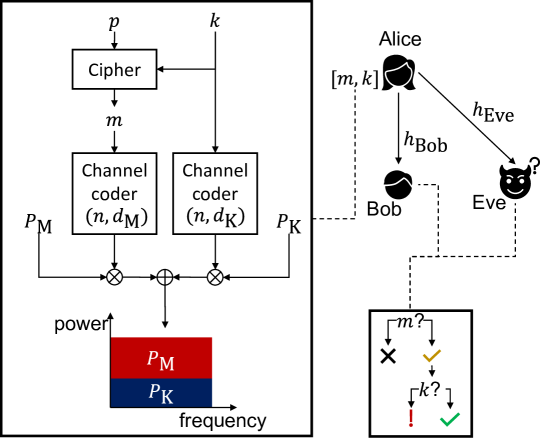
Figure 1: System model

II-B Error and Utility Models

Considering a finite blocklength $n$ for both packets, we adopt the Polyanskiy bound [8] to characterize the error rate in FBL regime. Given a $n$-symbol codeword of $d$ bits payload, the packet error rate (PER) is upper-bounded by $\varepsilon=Q\left[\sqrt{\frac{n}{V}}\left(\eta-\frac{d}{n}\right)\ln 2\right]$, where $Q(x)=\frac{1}{2}\text{erfc}\left(\frac{x}{\sqrt{2}}\right)$ is the Gaussian tail distribution function, $\gamma$ is the signal-to-interference-and-noise ratio (SINR), and $V$ is the channel dispersion. For AWGN channels, $V(\gamma)=1-\frac{1}{(1+\gamma)^{2}}$. $\eta=\frac{\mathcal{C}}{B}$ is the spectral efficiency, where $\mathcal{C}=B\log_{2}(1+\gamma)$ is the Shannon capacity. For FBL, we usually normalize the bandwidth to $B=1$ for convenience of analysis, so that

$$\varepsilon=Q\left[\sqrt{\frac{n}{V(\gamma)}}\left(\mathcal{C}-\frac{d}{n}\right)\ln 2\right].$$ (2)

For both $i\in\{\emph{Bob},\emph{Eve}\}$, the SIC begins with decoding the message $m$, where the key $k$ plays the role of interference. Thus, the SINR is $\gamma_{i,\text{M}}=\frac{z_{i}P_{\mathrm{M}}}{z_{i}P_{\mathrm{K}}+\sigma^{2}}$ and the PER is

$$\epsilon_{i,\text{M}}=\varepsilon_{i,\text{M}}=Q\left[\sqrt{\frac{n}{V(\gamma_{i,\text{M}})}}\left(\mathcal{C}_{i,\text{M}}-\frac{d_{\mathrm{M}}}{n}\right)\ln 2\right].$$ (3)

Upon a successful decoding of $m$, $i$ can carry out the SIC, and therewith further decode $k$ without being interfered by $m$. In this case, the signal-to-noise ratio (SNR) is $\gamma_{i,\text{K}}=\frac{z_{i}P_{\mathrm{K}}}{\sigma^{2}}$ and the PER is

$$\varepsilon_{i,\text{K}}=Q\left[\sqrt{\frac{n}{V(\gamma_{i,\text{K}})}}\left(\mathcal{C}_{i,\text{K}}-\frac{d_{\mathrm{K}}}{n}\right)\ln 2\right].$$ (4)

Alternatively, in case the decoding of $m$ fails, $i$ can also attempt to directly decode $k$ under the interference from $m$, where the SINR is $\gamma^{\prime}_{i,\text{K}}=\frac{z_{i}P_{\mathrm{K}}}{z_{i}P_{\mathrm{M}}+\sigma^{2}}$ and the PER is

$$\varepsilon^{\prime}_{i,\text{K}}=Q\left[\sqrt{\frac{n}{V(\gamma^{\prime}_{i,\text{K}})}}\left(\mathcal{C}_{i,\text{K}}-\frac{d_{\mathrm{K}}}{n}\right)\ln 2\right].$$ (5)

Thus, the overall error probability in decoding $k$ is

$$\epsilon_{i,\text{K}}=(1-\varepsilon_{i,\text{M}})\varepsilon_{i,\text{K}}+\varepsilon_{i,\text{M}}\varepsilon^{\prime}_{i,\text{K}}.$$ (6)

As we force $P_{\mathrm{M}}>P_{\mathrm{K}}$, it always holds that $\gamma^{\prime}_{i,\text{K}}<$0\text{\,}\mathrm{dB}$$. The direct decoding of $k$ without SIC is therefore unlikely to succeed due to the strong interference, i.e. we can approximately consider $\varepsilon^{\prime}_{i,\text{K}}\approx 1$. Moreover, following the classical FBL approach we neglect the second-order error term $\varepsilon_{i,\text{M}}\varepsilon_{i,\text{K}}\approx 0$. Applying both approximations on Eq. (6), we have

$$\epsilon_{i,\text{K}}\approx\varepsilon_{i,\text{K}}+\varepsilon_{i,\text{M}}.$$ (7)

The expected utility received by both $i\in\{\emph{Bob},\emph{Eve}\}$ is

$$\begin{split}\mathbb{E}\{U_{i}\}=&\left(1-\epsilon_{i,\text{M}}\right)\left(1-\epsilon_{i,\text{K}}\right)-\left(1-\epsilon_{i,\text{M}}\right)\epsilon_{i,\text{K}}\\ =&\left(1-\epsilon_{i,\text{M}}\right)\left(1-2\epsilon_{i,\text{K}}\right),\end{split}$$ (8)

and we consider the system’s overall utility $U_{\Sigma}=U_{\emph{Bob}}-U_{\emph{Eve}}$.

II-C Strategy Optimization

Now consider a fixed power budget $P_{\Sigma}\in(0,+\infty)$ of Alice, a fixed packet size $n$, and a fixed payload message length $d_{\mathrm{M}}$. We look for an optimal strategy of encryption coding and power allocation that maximizes the system utility: [2] d_K, P_M, P_K E{U_Σ} P_M⩾0 P_K⩾0 P_M+P_K⩽P_Σ d_K∈{0,1,…n} ϵ_Bob,M⩽ϵ^th_Bob,M ϵ_Eve,M⩽ϵ^th_Eve,M ϵ_Bob,K⩽ϵ^th_Bob,K ϵ_Eve,K⩾ϵ^th_Eve,K, where $\epsilon^{\mathrm{th}}_{\emph{Bob},\text{M}}$, $\epsilon^{\mathrm{th}}_{\emph{Eve},\text{M}}$, $\epsilon^{\mathrm{th}}_{\emph{Bob},\text{K}}$, and $\epsilon^{\mathrm{th}}_{\emph{Eve},\text{K}}$ are pre-fixed thresholds of error probability.

III Proposed Approach

While the multivariate program (II-C) is hard to tract, we can derive the following lemma and theorems to reduce its complexity. The detailed proofs are provided in the appendices.

Theorem 1.

With $\epsilon_{\emph{Bob},\text{M}}<0.5$, $\epsilon_{\emph{Eve},\text{M}}<0.5$, and $P_{\Sigma}<+\infty$, given any $d_{\mathrm{K}}$, the optimal power allocation $P^{\mathrm{o}}_{\mathrm{M}}$ and $P^{\mathrm{o}}_{\mathrm{K}}$ must fulfill $P^{\mathrm{o}}_{\mathrm{M}}+P^{\mathrm{o}}_{\mathrm{K}}=P_{\Sigma}$.

Driven by Theorem 1, we define the expected $U_{\Sigma}$ under full-power transmission as $U_{\mathrm{FP}}\triangleq\mathbb{E}\{U_{\Sigma}|{P_{\mathrm{K}}=P_{\Sigma}-P_{\mathrm{M}}}\}$, and Problem (II-C) is degraded to bivariate: [2] d_M, P_MU_FP P_K∈[0,P_Σ] constraints (II-C)–(II-C). However, Problem (1) is still a mixed integer non-convex problem, which is difficult to solve. To tackle this issue, we relax $d_{\mathrm{K}}$ from integer into a real value, i.e., $0\leqslant d_{\mathrm{K}}\leqslant n$. Then, we leverage the block coordinate descent (BCD) framework to obtain the corresponding solutions iteratively.

In particular, in each $t^{\mathrm{th}}$ iteration, we fix the bit length of key as $d_{\mathrm{K}}=d^{(t-1)}_{\mathrm{K}}$. Then, Problem (1) is reformulated as[2] P_MU_FP P_M∈[0,P_Σ]d_K=d^(t-1)_K constraints (II-C)–(II-C). Note that $U_{\mathrm{FP}}$ consists of the multiplications and subtraction of PERs for both $m$ and $k$. Thus, we first characterize their convexity and monotonicity with the following Lemma:

Lemma 1.

With $\epsilon_{\emph{Bob},\text{M}}<0.5$, $\epsilon_{\emph{Eve},\text{M}}<0.5$, and $P_{\Sigma}<+\infty$, both $\epsilon_{\emph{Bob},\text{M}}$ and $\epsilon_{\emph{Eve},\text{M}}$ are strictly monotonically decreasing and convex of $P_{\mathrm{M}}$ in the feasible region of Problem (1).

Therewith, the constraints (II-C)–(II-C) are convex while the rest of them being affine. Furthermore, we can establish the following partial concavity of the utility $U_{\mathrm{FP}}$:

Theorem 2.

$U_{\mathrm{FP}}$ is concave of $P_{\mathrm{M}}$ in the feasible region of Problem (1).

As a result, Problem (1) is concave and can be solved efficiently with any standard convex optimization tool. Denoting its optimum $P^{(t)}_{\mathrm{M}}$, we fix $P_{\mathrm{M}}=P^{(t)}_{\mathrm{M}}$ in Problem (1) as: [2] d_KU_FP d_K∈[0,n] P_M=P^(t)_M constraints (II-C)–(II-C). We can also identify the following partial concavity of $U_{\mathrm{FP}}$:

Theorem 3.

If $\epsilon^{\mathrm{th}}_{\emph{Bob},\text{K}}\leqslant 0.5$ and $\epsilon^{\mathrm{th}}_{\emph{Eve},\text{K}}\geqslant 0.5$, $U_{\mathrm{FP}}$ is concave of $d_{\mathrm{K}}$ in the feasible region of Problem (1).

Accordingly, Problem (2) can be solved as a concave problem, since the objective function is concave and the constraints are convex or affine. We denote the optimal solution of Problem (2) as $d^{(t)}_{\mathrm{K}}$, which is set as the fixed value of $d_{\mathrm{K}}$ is the $(t+1)^{\mathrm{th}}$ iteration. Moreover, its corresponding optimal value is denoted as $U^{(t)}_{\mathrm{LF}}=U_{LF}(P^{(t)}_{\mathrm{M}},d^{(t)}_{\mathrm{K}})$. This process will repeat until it meets either the stop criterion $\left|U^{(t)}-U^{(t-1)}\right|\leqslant\mu$ or a given maximal allowed iteration rounds $T$, where $\mu$ is a non-negative threshold. The obtained solutions are denoted as $P^{*}_{\mathrm{K}}$ and $d^{*}_{\mathrm{K,R}}$, respectively. Specially, we initialize the variable pair as $\left(d^{(0)}_{\mathrm{K}},P^{(0)}_{\mathrm{M}}\right)=\left(d^{\mathrm{init}}_{\mathrm{K}},P^{\mathrm{init}}_{\mathrm{M}}\right)$ and the obtained utility $U^{(0)}_{\mathrm{FP}}=-\infty$. It should be emphasized that the initial value $(d^{\mathrm{init}}_{\mathrm{K}},P^{\mathrm{init}}_{\mathrm{M}})$ must be feasible for Problem (1). Recalling that $d_{\mathrm{K}}$ must be integer, the optimal integer solution shall be obtained via comparing the integer neighbors of $d^{*}_{\mathrm{K,R}}$:

$$d^{*}_{\mathrm{K}}=\arg\max\limits_{m\in\left\{\left\lfloor d^{*}_{\mathrm{K,R}}\right\rfloor,\left\lceil d^{*}_{\mathrm{K,R}}\right\rceil\right\}}U_{\mathrm{LF}}(P^{*}_{\mathrm{M}}).$$ (9)

The BCD framework to solve Problem (1) can be described by Algorithm 1. It is able to achieve sub-optimal solutions with the complexity of $\mathcal{O}(\phi(4N^{2}))$, where $N$ is the number of variables in Problem (1) and $\phi(\cdot)$ represents the iteration numbers upon the solution accuracy [9].

1 Input: $\mu,T,P_{\Sigma},d_{\mathrm{M}},n$

2 Initialize: $t=1,P^{\mathrm{0}}_{\mathrm{M}}=P^{\mathrm{init}}_{\mathrm{M}},d^{\mathrm{0}}_{\mathrm{K}}=d^{\mathrm{init}}_{\mathrm{K}},U^{\mathrm{o}}_{\mathrm{FP}}=-\infty$

3 do // Check convergence

4       if $t\leqslant T$ then // Limiting the number of iterations

5             $P^{(t)}_{\mathrm{M}}\leftarrow\arg\max\limits_{P_{\mathrm{M}}}U_{\mathrm{FP}}\left(d^{(t-1)}_{\mathrm{K}},P_{\mathrm{M}}\right)$ $d^{(t)}_{\mathrm{K}}\leftarrow\arg\max\limits_{d_{\mathrm{K}}}U_{\mathrm{FP}}\left(d_{\mathrm{K}},P^{(t)}_{\mathrm{M}}\right)$

6             $U^{(t)}_{\mathrm{FP}}\leftarrow U_{\mathrm{FP}}\left(d^{(t)}_{\mathrm{K}},P^{(t)}_{\mathrm{M}}\right)$

7             $t\leftarrow t+1$

8            

9       else

10            break

11       end if

12      

13while $|U^{(t)}-U^{(t-1)}|\geqslant\xi$

14$P^{*}_{\mathrm{K}}\leftarrow P^{(t)}_{\mathrm{K}}$

15$d^{*}_{\mathrm{K,R}}\leftarrow\arg\max\limits_{m\in\left\{\left\lfloor d^{(t)}_{\mathrm{K}}\right\rfloor,\left\lceil d^{(t)}_{\mathrm{K}}\right\rceil\right\}}U_{\mathrm{LF}}(P^{(t)}_{\mathrm{M}})$

return $\left(d^{*}_{\mathrm{K}},P^{*}_{\mathrm{M}}\right)$

Algorithm 1 The BCD framework

IV Numerical Verification

To verify our analyses and evaluate our proposed approach, we conducted a series of numerical simulations. All these simulations share the same setup listed in Tab. I. Task-specific configurations will be provided correspondingly later when we introduce each of them in details below.

TABLE I: Simulation setup

Parameter	Value	Remark
$\sigma^{2}$	$1\text{\,}\mathrm{mW}$	AWGN power
$z_{\emph{Bob}}$	$0\text{\,}\mathrm{dB}$	Channel gain of Bob
$B$	$1\text{\,}\mathrm{Hz}$	Normalized to unity bandwidth
$n$	64	Block length per packet
$\epsilon_{\emph{Bob},\text{M}}^{\mathrm{th}}$, $\epsilon_{\emph{Bob},\text{K}}^{\mathrm{th}}$, $\epsilon_{\emph{Eve},\text{K}}^{\mathrm{th}}$, $\epsilon_{\emph{Eve},\text{K}}^{\mathrm{th}}$	0.5	Threshold in constraints (II-C)–(II-C)
$\xi$	$2\times 10^{-16}$	BCD convergence threshold
$K$	100	Maximal number of iterations in BCD

IV-A Superiority of Full-Power Transmission

First, to verify Theorem 1 that the optimal power allocation always fully exploits the power budget $P_{\Sigma}$, we set $P_{\Sigma}=$10\text{\,}\mathrm{mW}$$, $z_{\emph{Eve}}=$-10\text{\,}\mathrm{dB}$$, $d_{\mathrm{M}}=16$, and computed $\mathbb{E}\{U_{\Sigma}\}$ w.r.t. Eq. (8) in the region $(P_{\mathrm{M}},P_{\mathrm{K}})\in[0,$10\text{\,}\mathrm{mW}$]^{2}$. For each $P_{\mathrm{M}}$ in the feasible region of Problem (II-C), we executed exhaustive search to find the optimal $P^{\mathrm{o}}_{\mathrm{K}}$ that maximizes $\mathbb{E}\{U_{\Sigma}\}$. We carried out this test twice, with different settings of the ciphering key length $d_{\mathrm{K}}$: once with 30 bits and once with 60 bits. As the results illustrated in Fig. 2 reveal, in both cases, all optimal power allocations land on the full-power boundary $P_{\mathrm{M}}+P_{\mathrm{K}}=P_{\Sigma}$, which supports our analysis.

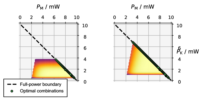
Figure 2: The optimal selection of $P_{\mathrm{M}}$ upon different specifications of $P_{\mathrm{K}}$, with $d_{\mathrm{K}}=30$ (left) and $d_{\mathrm{K}}=60$ (right).

IV-B Utility Surface

To obtain insights about the overall surface of system utility $U_{\mathrm{FP}}$ under the strategy of full-power transmission, we set $P_{\Sigma}=$10\text{\,}\mathrm{mW}$$, $z_{\emph{Eve}}=$-10\text{\,}\mathrm{dB}$$, $d_{\mathrm{M}}=16$, and computed $U_{\mathrm{FP}}$ in the region $(P_{\mathrm{M}},d_{\mathrm{K}})\in[0,$10\text{\,}\mathrm{mW}$]\times\{0,1,\dots 64\}$. The result is depicted in Fig. 3, where the feasible region outlined by (II-C)–(II-C) is highlighted with higher opacity w.r.t. the rest parts. We can observe from the figure that $U_{\mathrm{FP}}$ is concave of both $P_{\mathrm{M}}$ and $d_{\mathrm{K}}$ within the feasible region, while the convexity/concavity outside the region is rather complex.

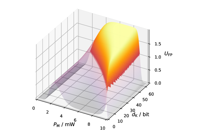
Figure 3: The system utility $U_{\mathrm{FP}}$ under full-power transmission

IV-C Convergence Test of the BCD Framework

To monitor the feasibility of the proposed BCD framework in the joint optimization of the encryption coding and power allocation, we set $P_{\Sigma}=$10\text{\,}\mathrm{mW}$$, $z_{\emph{Eve}}=$-10\text{\,}\mathrm{dB}$$, and tested our Algorithm 1 with two sample configurations of the payload message bit length: $d_{\mathrm{M}}=16$ and $d_{\mathrm{M}}=24$. As the results shown in Fig. 4 are suggesting, the BCD algorithm efficiently converges in both cases, and successfully achieves the global optima after 8 and 9 iterations, respectively.

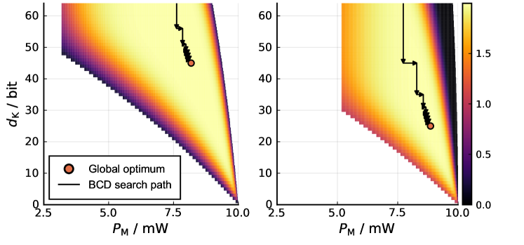
Figure 4: The $U_{\mathrm{FP}}$ surface and the search path of Algorithm 1, with $d_{\mathrm{M}}=16$ (left) and $d_{\mathrm{M}}=24$ (right).

IV-D Performance Evaluation

To assess the security level and deceiving capability of our proposed approach, we are interested in two different performance indicators of it. Regarding secured transmission, we consider the secure reliability

$$R_{\mathrm{s}}=(1-\epsilon_{\emph{Bob}})\epsilon_{\emph{Eve}},$$ (10)

where $\epsilon_{i}=1-(1-\epsilon_{i,\text{M}})(1-\epsilon_{i,\text{K}})$ is the overall error rate in decoding the payload message for both $i\in\{\emph{Bob},\emph{Eve}\}$. Regarding deception, we consider the effective deception rate

$$R_{\mathrm{d}}=(1-\delta_{\emph{Bob}})\delta_{\emph{Eve}},$$ (11)

where $\delta_{i}=(1-\epsilon_{i,\text{M}})\epsilon_{i,\text{K}}$ is the probability that $i\in\{\emph{Bob},\emph{Eve}\}$ is deceived to obtain an incorrect payload.

First we set $P_{\Sigma}=$3\text{\,}\mathrm{mW}$$, $d_{\mathrm{M}}=16$, and measured $U_{\mathrm{FP}}$, $R_{\mathrm{s}}$, as well as $R_{\mathrm{d}}$ under different conditions of $z_{\emph{Eve}}$. As a baseline to compare with, we also implemented a classical secure-reliability-optimal PLS solution without the deceiving mechanism, i.e., we set $d_{\mathrm{K}}=0$, $P_{\mathrm{K}}=0$, and chose the optimal $P_{\mathrm{M}}\in[0,P_{\Sigma}]$ that maximizes $R_{\mathrm{s}}$. The results are shown in Fig. 5. Compared to the baseline solution, our approach offers a significant enhancement in the robustness of $R_{s}$ against increasing $z_{\emph{Eve}}$. When Eve has a poor channel with $-10\text{\,}\mathrm{dB}$ gain, our solution compromises only slightly regarding the secure reliability, by less than $3\%$ compared to the baseline, while delivering a high effective deception rate over $80\%$. Moreover, the deception rate may even benefit from a good channel condition of Eve (since Eve is in this case more likely to decode the message packet), exceeding $98\%$ around $z_{\emph{Eve}}=$-7\text{\,}\mathrm{dB}$$.

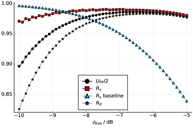
Figure 5: Results of sensitivity test regarding $z_{\emph{Eve}}$

Then we fixed $z_{\emph{Eve}}=$-5\text{\,}\mathrm{dB}$$ and repeated the assessment under different power budgets $P_{\Sigma}$, whereby we obtained the results in Fig. 6. Again, with sufficient power budget, we observe a significant enhancement in secure reliability w.r.t. the baseline, in addition to a high effective deception rate. Moreover, in contrast to the classical PLS solutions that cannot benefit from higher power budget, our approach can be overall enhanced in various aspects of performance by raising $P_{\Sigma}$.

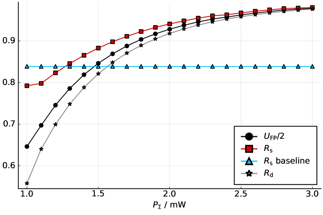
Figure 6: Results of sensitivity test regarding $P_{\Sigma}$

Results of a more comprehensive benchmark test, which mixes different settings of $z_{\emph{Eve}}$ and $P_{\Sigma}$, are illustrated in Fig. 7. It reveals that our approach generally outperforms the baseline of classical PLS regarding the secured reliability, as long as supported by a sufficient power budget. More specifically, the minimal $P_{\Sigma}$ required for our solution to outperform the baseline increases along with the channel gain gap $z_{\emph{Bob}}-z_{\emph{Eve}}$. In addition, it is worth to discuss the case when $z_{\emph{Eve}}=$-3\text{\,}\mathrm{dB}$$ and $P_{\Sigma}\geqslant$2.7\text{\,}\mathrm{mW}$$, where no feasible solution with full-power transmission can be found under the constraints (II-C) – (II-C). In such cases, we suggest to either take a sub-optimal solution with lower transmission power that $P_{\mathrm{M}}+P_{\mathrm{K}}<P_{\Sigma}$, or adjust the blocklength $n$ of each packet.

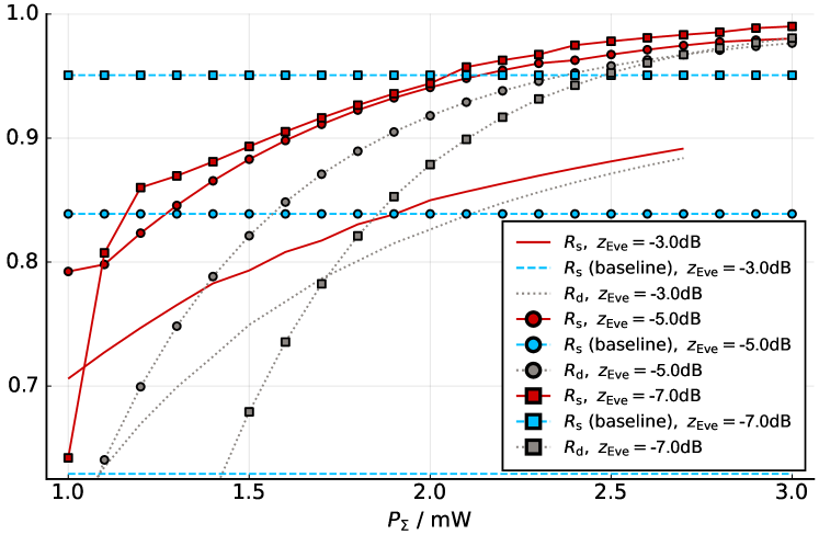
Figure 7: Benchmark results

V Conclusion and Outlooks

In this paper, we have proposed a novel security framework to enhance the classical PLS approach with the capability of deceiving eavesdroppers, and provided a solution to jointly optimize its encryption coding rate and power allocation. With numerical results we have demonstrated the effectiveness of our methods. Compared to conventional PLS approaches, our proposal exhibits a unique feature of benefiting from higher transmission power budget, which makes it superior when confronting eavesdroppers with good channels.

As a pioneering research, this work can be extended in multiple directions. First, the migration of our proposed framework to orthogonal multiplexing is of great interest. Second, the issue that the feasible region vanishes under good eavesdropping channel and high power budget shall be addressed. Third, a more generic and flexible solution can be achieved by modifying the objective and constraints of the optimization problem. Furthermore, specific design of the encryption codec must be investigated to efficiently realize our approach.

Appendix A Proof of Theorem 1

Proof.

This theorem can be proven straightforwardly by the contradiction. Given a certain $d_{\mathrm{K}}$, in this appendix we can use the following notations for convenience:

$$\overline{U}_{\Sigma}(P_{1},P_{2})\triangleq\mathbb{E}\left\{U_{\Sigma}|P_{\mathrm{M}}=P_{1},P_{\mathrm{K}}=P_{2}\right\},$$ (12)

$$\epsilon_{i,j}(P)\triangleq\epsilon_{i,j}|_{P_{j}=P},\quad\forall(i,j)\in\{\emph{Bob},\emph{Eve}\}\times\{\text{M},\text{K}\}.$$ (13)

Suppose there exists an optimal power allocation $\left(P^{\mathrm{o}}_{\mathrm{K}},P^{\mathrm{o}}_{\mathrm{M}}\right)$ that leaves from the power budget a positive residual $P_{\Delta}=P_{\Sigma}-P^{\mathrm{o}}_{\mathrm{K}}-P^{\mathrm{o}}_{\mathrm{M}}>0$. Since it is optimal, for all feasible $\left(P^{\prime}_{\mathrm{M}},P^{\prime}_{\mathrm{K}}\right)\neq\left(P^{\mathrm{o}}_{\mathrm{K}},P^{\mathrm{o}}_{\mathrm{M}}\right)$ it must hold that

$$\overline{U}_{\Sigma}\left(P^{\mathrm{o}}_{\mathrm{M}},P^{\mathrm{o}}_{\mathrm{K}}\right)\geqslant\overline{U}_{\Sigma}\left(P^{\prime}_{\mathrm{M}},P^{\prime}_{\mathrm{K}}\right).$$ (14)

Meanwhile, there is always another feasible allocation $(P^{\mathrm{f}}_{\mathrm{M}},P^{\mathrm{o}}_{\mathrm{K}})$ where $P^{\mathrm{f}}_{\mathrm{M}}=P^{\mathrm{o}}_{\mathrm{M}}+P_{\Delta}$. Given the same $P_{\mathrm{K}}$, it is trivial to see that $\epsilon_{\emph{Bob},\text{M}}$ and $\epsilon_{\emph{Eve},\text{M}}$ are monotonically decreasing in $P_{\mathrm{M}}$, so it always holds that

$$\epsilon_{\emph{Bob},\text{M}}(P^{\mathrm{o}}_{\mathrm{M}}) >\epsilon_{\emph{Bob},\text{M}}\left(P^{\mathrm{f}}_{\mathrm{M}}\right),$$ (15)

$$\epsilon_{\emph{Eve},\text{M}}(P^{\mathrm{o}}_{\mathrm{M}}) >\epsilon_{\emph{Eve},\text{M}}\left(P^{\mathrm{f}}_{\mathrm{M}}\right)$$ (16)

Therefore, we have:

$$\begin{split}&\overline{U}_{\Sigma}\left(P^{\mathrm{f}}_{\mathrm{M}},P^{\mathrm{o}}_{\mathrm{K}}\right)-\overline{U}_{\Sigma}\left(P^{\mathrm{o}}_{\mathrm{M}},P^{\mathrm{o}}_{\mathrm{K}}\right)\\ =&\left[1-2\epsilon_{\emph{Bob},\text{K}}\left(P^{\mathrm{o}}_{\mathrm{K}}\right)\right]\left[\epsilon_{\emph{Bob},\text{M}}\left(P^{\mathrm{o}}_{\mathrm{M}}\right)-\epsilon_{\emph{Bob},\text{M}}\left(P^{\mathrm{f}}_{\mathrm{M}}\right)\right]\\ &-\left[1-2\epsilon_{\emph{Eve},\text{K}}\left(P^{\mathrm{o}}_{\mathrm{K}}\right)\right]\left[\epsilon_{\emph{Eve},\text{M}}\left(P^{\mathrm{o}}_{\mathrm{M}}\right)-\epsilon_{\emph{Eve},\text{M}}\left(P^{\mathrm{f}}_{\mathrm{M}}\right)\right]\\ >&0.\end{split}$$ (17)

The inequality above holds, since $2\epsilon_{\emph{Bob},\text{K}}\leqslant 2\epsilon^{\mathrm{th}}_{\emph{Bob},\text{K}}<1$ and $2\epsilon_{\emph{Eve},\text{K}}\geqslant 2\epsilon^{\mathrm{th}}_{\emph{Eve},\text{K}}>1$. In other words, the solution $P^{\mathrm{f}}_{\mathrm{K}}$ and $P^{\mathrm{f}}_{\mathrm{M}}$ achieves a better utility $\overline{U}_{\Sigma}\left(P^{\mathrm{f}}_{\mathrm{M}},P^{\mathrm{o}}_{\mathrm{K}}\right)$ than $\overline{U}_{\Sigma}\left(P^{\mathrm{o}}_{\mathrm{M}},P^{\mathrm{o}}_{\mathrm{K}}\right)$, which violates the assumption of optimum. ∎

Appendix B Proof of Lemma 1

Proof.

For the sake of clarity, we define an auxiliary function $\omega(\gamma)\triangleq\sqrt{\frac{n}{V(\gamma)}}\left[\mathcal{C}(\gamma)-\frac{d}{n}\right]$. In [10, 3], we have shown that $\omega$ is monotonically decreasing and convex of the S(I)NR $\gamma$, i.e.,

$$\begin{split}&\frac{\partial{\omega}}{\partial{\gamma}}\\ =&\sqrt{\frac{n}{V}}\left[\frac{\gamma^{2}+2\gamma-\ln(\gamma+1)}{(\gamma^{2}+2\gamma)(\gamma+1)}+\frac{d}{2V}\frac{2}{(1+\gamma)^{3}}\right]\geqslant 0,\end{split}$$ (18)

$$\frac{\partial^{2}\omega}{\partial\gamma^{2}}\leqslant\sqrt{\frac{n}{[\gamma(\gamma+2)]^{5}}}\left[0-3\ln{2}\cdot(\gamma+1)\frac{d}{n}\right]\leqslant 0.$$ (19)

Moreover, it is clear that the FBL error probability itself, i.e., $\varepsilon$ in Eq. (2), is decreasing and convex of $\omega$ if $\mathcal{C}-\frac{d}{n}\geqslant 0$, otherwise it is decreasing and concave if $\mathcal{C}-\frac{d}{n}\leqslant 0$. This can be verified straightforwardly with $\frac{\partial\varepsilon}{\partial\omega}=-\frac{1}{\sqrt{2\pi}}e^{-\frac{\omega^{2}}{2}}\leqslant 0$ and $\frac{\partial^{2}\varepsilon}{\partial\omega^{2}}$. Since $\epsilon_{i,\text{M}}=\varepsilon_{i,\text{M}}$ as given by Eq. (3), all aforementioned conclusions regarding $\varepsilon$ also hold for $\epsilon_{i,\text{M}}$ with both $i\in\{\emph{Bob},\emph{Eve}\}$. With $P_{\mathrm{M}}+P_{\mathrm{K}}=P_{\Sigma}$, we have

$$\begin{split}&\frac{\partial\gamma_{i,\text{M}}}{\partial P_{\mathrm{M}}}=\frac{\partial}{\partial P_{\mathrm{M}}}\left(\frac{z_{i}P_{\mathrm{M}}}{z_{i}(P_{\Sigma}-P_{\mathrm{M}})+\sigma^{2}}\right)\\ =&\frac{z_{i}(z_{i}P_{\Sigma}+\sigma^{2})}{(z_{i}P_{\mathrm{K}}+\sigma^{2})^{2}}>0,\end{split}$$ (20)

$$\frac{\partial^{2}\gamma_{i,\text{M}}}{\partial P^{2}_{\mathrm{M}}}=\frac{2z_{i}^{2}(z_{i}P_{\Sigma}+\sigma^{2})}{(z_{i}P_{\mathrm{K}}+\sigma^{2})^{3}}>0,$$ (21)

$$\frac{\partial\epsilon_{i,\text{M}}}{\partial P_{\mathrm{M}}}=\frac{\partial\epsilon_{i,\text{M}}}{\partial\omega_{i,\text{M}}}\frac{\partial\omega_{i,\text{M}}}{\partial\gamma_{i,\text{M}}}\frac{\partial\gamma_{i,\text{M}}}{\partial P_{\mathrm{M}}}\leqslant 0$$ (22)

Especially, the equity in Eq. (22) is achieved only when $\omega_{i,\text{M}}\to+\infty$ and $\gamma_{i,\text{M}}\to+\infty$, i.e. $P_{\mathrm{M}}\to\infty$. So given a limited $0<P_{\Sigma}<+\infty$, it always holds $\frac{\partial\epsilon_{i,\text{M}}}{\partial P_{\mathrm{M}}}<0$, i.e. $\epsilon_{i,\text{M}}$ is strictly monotonically decreasing of $P_{\mathrm{M}}$.

Moreover, since $n\geqslant 10$ and $\epsilon_{i,\text{M}}\leqslant\epsilon^{\mathrm{th}}_{i,\text{M}}<0.5$, there is

$$\begin{split}&\frac{\partial^{2}\epsilon_{i,\text{M}}}{\partial P_{\mathrm{M}}^{2}}=\frac{\partial\epsilon_{i,\text{M}}}{\partial\gamma_{i,\text{M}}}\frac{\partial^{2}\gamma_{i,\text{M}}}{\partial P_{\mathrm{M}}^{2}}+\frac{\partial^{2}\epsilon_{i,\text{M}}}{\partial\gamma^{2}_{i,\text{M}}}\left(\frac{\partial\gamma_{i,\text{M}}}{\partial P_{\mathrm{M}}}\right)^{2}\\ =&\frac{1}{\sqrt{2\pi}}e^{-\frac{\omega_{i,\text{M}}}{2}}\left(\frac{\partial\omega_{i,\text{M}}}{\partial\gamma_{i,\text{M}}}\left(\omega_{i,\text{M}}\frac{\partial\omega_{i,\text{M}}}{\partial\gamma_{i,\text{M}}}\left(\frac{\partial\gamma_{i,\text{M}}}{\partial P_{\mathrm{M}}}\right)^{2}-\frac{\partial^{2}\gamma_{i,\text{M}}}{\partial P_{\mathrm{M}}^{2}}\right)-\underbrace{\frac{\partial^{2}\omega_{i,\text{M}}}{\partial\gamma^{2}_{i,\text{M}}}\left(\frac{\partial\gamma_{i,\text{M}}}{\partial P_{\mathrm{M}}}\right)^{2}}_{\leqslant 0}\right)\\ \geqslant&\frac{1}{\sqrt{2\pi}}e^{-\frac{\omega_{i,\text{M}}}{2}}\frac{\partial\omega_{i,\text{M}}}{\partial\gamma_{i,\text{M}}}\left(\omega_{i,\text{M}}\frac{\partial\omega_{i,\text{M}}}{\partial\gamma_{i,\text{M}}}\left(\frac{\partial\gamma_{i,\text{M}}}{\partial P_{\mathrm{M}}}\right)^{2}-\frac{\partial^{2}\gamma_{i,\text{M}}}{\partial P_{\mathrm{M}}^{2}}\right)\\ =&\frac{1}{\sqrt{2\pi}}e^{-\frac{\omega_{i,\text{M}}}{2}}\frac{\partial\omega_{i,\text{M}}}{\partial\gamma_{i,\text{M}}}\left(\omega_{i,\text{M}}\frac{\partial\omega_{i,\text{M}}}{\partial\gamma_{i,\text{M}}}\frac{z^{2}_{1}(z_{i}P_{\Sigma}+\sigma^{2}_{i})^{2}}{(z_{i}P_{\mathrm{K}}+\sigma^{2}_{i})^{4}}-\frac{2z_{i}^{2}(z_{i}P_{\Sigma}+\sigma^{2}_{i})}{(z_{i}P_{\mathrm{K}}+\sigma^{2}_{i})^{3}}\right)\\ =&\frac{1}{\sqrt{2\pi}}e^{-\frac{\omega_{i,\text{M}}}{2}}\frac{\partial\omega_{i,\text{M}}}{\partial\gamma_{i,\text{M}}}\frac{z_{i}^{2}(z_{i}P_{\Sigma}+\sigma^{2}_{i})}{(z_{i}P_{\mathrm{K}}+\sigma^{2}_{i})^{3}}\left(\omega_{i,\text{M}}\frac{\partial\omega_{i,\text{M}}}{\partial\gamma_{i,\text{M}}}\underbrace{\frac{(z_{i}P_{\Sigma}+\sigma^{2}_{i})}{(z_{i}P_{\mathrm{K}}+\sigma^{2}_{i})}}_{\geqslant\gamma_{i,\text{M}}}-2\right)\\ \geqslant&\frac{1}{\sqrt{2\pi}}e^{-\frac{\omega_{i,\text{M}}}{2}}\frac{\partial\omega_{i,\text{M}}}{\partial\gamma_{i,\text{M}}}\frac{z_{i}^{2}(z_{i}P_{\Sigma}+\sigma^{2}_{i})}{(z_{i}P_{\mathrm{K}}+\sigma^{2}_{i})^{3}}\left(\omega_{i,\text{M}}\frac{\partial\omega_{i,\text{M}}}{\partial\gamma_{i,\text{M}}}\gamma_{i,\text{M}}-2\right)\geqslant\frac{6.25\gamma_{i,\text{M}}}{\sqrt{\gamma_{i,\text{M}}(\gamma_{i,\text{M}}+1)}}-2\geqslant 0,\end{split}$$ (23)

i.e. $\epsilon_{i,\text{M}}$ is convex of $P_{\mathrm{M}}$. The inequality holds with $\gamma_{i,M}\geq\gamma_{th}\geq 1$, which is required to fulfill the error probability constraints in practical scenarios [10]. ∎

Appendix C Proof of Theorem 3

Proof.

The second derivative of $U_{\mathrm{FP}}$ w.r.t. $d_{\mathrm{K}}$ is given by:

$$\begin{split}\frac{\partial^{2}U}{\partial d^{2}_{\mathrm{K}}}=&2(1-\epsilon_{\emph{Eve},\text{M}})\frac{\partial^{2}\epsilon_{\emph{Eve},\text{K}}}{\partial d^{2}_{\mathrm{K}}}\\ &+2(1-\epsilon_{\emph{Bob},\text{M}})\frac{\partial^{2}(-\epsilon_{\emph{Bob},\text{K}})}{\partial d^{2}_{\mathrm{K}}},\end{split}$$ (24)

where

$$\frac{\partial^{2}\epsilon_{\emph{Eve},\text{K}}}{\partial d^{2}_{\mathrm{K}}}=\frac{1}{mV_{\emph{Eve},\text{K}}}\underbrace{\frac{\partial^{2}\epsilon_{\emph{Eve},\text{K}}}{\partial\omega^{2}_{\emph{Eve},\text{K}}}}_{\leqslant 0}\leqslant 0,$$ (25)

$$\frac{\partial^{2}(-\epsilon_{\emph{Bob},\text{K}})}{\partial d^{2}_{\mathrm{K}}}=-\frac{1}{mV_{\emph{Eve},\text{K}}}\underbrace{\frac{\partial^{2}\epsilon_{\emph{Bob},\text{K}}}{\partial\omega^{2}_{\emph{Bob},\text{K}}}}_{\geqslant 0}\leqslant 0.$$ (26)

The above inequalities hold, since we have proven in [10] that $\frac{\partial^{2}\epsilon}{\partial\omega^{2}}\geqslant 0$, if $\epsilon\leqslant 0.5$ and $\frac{\partial^{2}\epsilon}{\partial\omega^{2}}\leqslant 0$, if $\epsilon\geqslant 0.5$. As a result, we have $\frac{\partial^{2}U_{\mathrm{FP}}}{\partial d^{2}_{\mathrm{K}}}\leqslant 0$ in the feasible region of Problem (1), which confirms the concavity. ∎

Appendix D Proof of Theorem 2

Proof.

We reformulate the utility $U_{\mathrm{FP}}$ and group its components as follows:

$$\begin{split}&U_{\mathrm{FP}}=U_{\emph{Bob}}-U_{\emph{Eve}}\\ =&(1-\epsilon_{\emph{Bob},\text{M}})-2(1-\epsilon_{\emph{Bob},\text{M}})\epsilon_{\emph{Bob},\text{K}}\\ &+2(1-\epsilon_{\emph{Eve},\text{M}})\epsilon_{\emph{Eve},\text{K}}-(1-\epsilon_{\emph{Eve},\text{M}})\\ =&\underbrace{(\epsilon_{\emph{Eve},\text{M}}-\epsilon_{\emph{Bob},\text{M}})}_{A_{1}}+\underbrace{2(\epsilon_{\emph{Eve},\text{M}}-\epsilon_{\emph{Bob},\text{M}})(\epsilon_{\emph{Eve},\text{M}}+\epsilon_{\emph{Bob},\text{M}}-1)}_{A_{2}}\\ &+2\underbrace{\left[(\epsilon_{\emph{Eve},\text{K}}-\epsilon_{\emph{Bob},\text{K}})+(\epsilon_{\emph{Bob},\text{M}}\epsilon_{\emph{Bob},\text{K}}-\epsilon_{\emph{Eve},\text{M}}\epsilon_{\emph{Eve},\text{K}})\right]}_{A_{3}}\end{split}$$ (27)

Note that $U_{\mathrm{FP}}$ is concave if each component $A_{k}$ where $k\in\{1,2,3\}$ are concave. Therefore, to this end we show the concavity of each $A_{k}$.

For $A_{1}$, we have already revealed with Lemma 1 the concavity of both $\epsilon_{i,\text{M}}$ w.r.t. $P_{\mathrm{M}}$ for both $i\in\{\emph{Bob},\emph{Eve}\}$. Moreover, $\epsilon_{i,\text{M}}$ is also monotonically decreasing in $z_{i}$ since

$$\begin{split}\frac{\partial\epsilon_{i,\text{M}}}{\partial z_{i}}&=\frac{\partial\epsilon_{i,\text{M}}}{\partial\gamma_{i}}\frac{\partial\gamma_{i}}{\partial z_{i}}=\frac{\partial\epsilon_{i,\text{M}}}{\partial\gamma_{i}}\frac{P_{\mathrm{M}}\sigma^{2}_{i}}{(z_{i}p_{m}+\sigma^{2}_{i})^{2}}\leqslant 0.\end{split}$$ (28)

Note that $\epsilon_{\emph{Eve},\text{M}}$ and $\epsilon_{\emph{Bob},\text{M}}$ actually distinguish from each other only regarding different values of $z_{i}$. Since we considerthat $z_{\emph{Bob}}\geqslant z_{\emph{Eve}}$, we have $A_{1}=\epsilon_{\emph{Eve},\text{M}}-\epsilon_{\emph{Bob},\text{M}}=\epsilon(P_{\mathrm{M}},z_{\emph{Eve}})-\epsilon(P_{\mathrm{M}},z_{\emph{Bob}})\geqslant 0$ and $\frac{\partial A^{2}_{1}}{\partial P_{\mathrm{M}}^{2}}=\frac{\partial^{2}\epsilon(P_{\mathrm{M}},z_{\emph{Eve}})}{\partial P_{\mathrm{M}}^{2}}-\frac{\partial^{2}\epsilon(P_{\mathrm{M}},z_{\emph{Bob}})}{\partial P_{\mathrm{M}}^{2}}\geqslant 0$.

For $A_{2}$, we have

$$\begin{split}\frac{\partial^{2}A_{2}}{\partial P_{\mathrm{M}}^{2}}=&\underbrace{\frac{\partial^{2}A_{1}}{\partial P_{\mathrm{M}}^{2}}}_{\geqslant 0}\underbrace{(\epsilon_{\emph{Eve},\text{M}}+\epsilon_{\emph{Bob},\text{M}}-1)}_{\leqslant 0}\\ &+\underbrace{A_{1}}_{\geqslant 0}\left(\underbrace{\frac{\partial^{2}\epsilon_{\emph{Eve},\text{M}}}{\partial P_{\mathrm{M}}^{2}}}_{\leqslant 0}+\underbrace{\frac{\partial^{2}\epsilon_{\emph{Bob},\text{M}}}{\partial P_{\mathrm{M}}^{2}}}_{\leqslant 0}\right)\\ &+2\underbrace{\frac{\partial A_{2}}{\partial P_{\mathrm{M}}}}_{\geqslant 0}\left(\underbrace{\frac{\partial\epsilon_{\emph{Eve},\text{M}}}{\partial P_{\mathrm{M}}}}_{\leqslant 0}+\underbrace{\frac{\partial\epsilon_{\emph{Bob},\text{M}}}{\partial P_{\mathrm{M}}}}_{\leqslant 0}\right)\leqslant 0.\end{split}$$ (29)

For $A_{3}$, first we note that due to the simple form of $\epsilon_{i,\text{K}}$ given by(7), all features of $\varepsilon$ regarding $\omega$ and $\gamma$ that we have proven in App. B also hold for $\epsilon_{i,\text{K}}$ with both $i\in\{\emph{Bob},\emph{Eve}\}$. However, albeit the term $\epsilon_{\emph{Eve},\text{K}}-\epsilon_{\emph{Bob},\text{K}}$ has the similar structure of $A_{1}$, the conclusion of concavity cannot be directly applied. This is due to the fact that we have $\epsilon_{\emph{Eve},\text{K}}\geqslant\epsilon^{\mathrm{th}}_{\emph{Eve},\text{K}}\geqslant 0.5$, which implies that $\epsilon_{\emph{Eve},\text{K}}$ is actually concave of $\omega_{\emph{Eve},\text{K}}$. Moreover, since the mask can only be decoded after SIC, the convexity of $\omega(\gamma_{i,\text{M}})$ w.r.t. $P_{\mathrm{M}}$ must also be revisited. In view of this, we first show that the $\epsilon_{\emph{Bob},\text{K}}$ is still convex of $P_{\mathrm{M}}$ with:

$$\begin{split}\frac{\partial^{2}\epsilon_{\emph{Bob},\text{K}}}{\partial P_{\mathrm{M}}^{2}}=&\frac{\partial^{2}\epsilon_{\emph{Bob},\text{K}}}{\partial\gamma^{2}_{\emph{Bob},\text{K}}}\left(\frac{\partial\gamma_{\emph{Bob},\text{K}}}{\partial P_{\mathrm{M}}}\right)^{2}=\frac{z^{2}_{\emph{Bob}}}{\sigma^{4}_{\emph{Bob}}}\underbrace{\frac{\partial^{2}\epsilon_{\emph{Bob},\text{K}}}{\partial\gamma^{2}_{\emph{Bob},\text{K}}}}_{\geqslant 0}\geqslant 0.\end{split}$$ (30)

Whilst, $\epsilon_{\emph{Eve},\text{K}}$ is concave of $P_{\mathrm{M}}$ since

$$\begin{split}\frac{\partial^{2}\epsilon_{\emph{Eve},\text{K}}}{\partial P_{\mathrm{M}}^{2}}=&\frac{\partial^{2}\epsilon_{\emph{Eve},\text{K}}}{\partial\omega^{2}_{\emph{Eve},\text{K}}}\left(\frac{\partial\omega_{\emph{Eve},\text{K}}}{\partial\gamma_{\emph{Eve},\text{K}}}\right)^{2}+\frac{\partial\epsilon_{\emph{Eve},\text{K}}}{\partial\omega_{\emph{Eve},\text{K}}}\frac{\partial^{2}\omega_{\emph{Eve},\text{K}}}{\partial\gamma^{2}_{\emph{Eve},\text{K}}}\leqslant 0.\end{split}$$ (31)

The inverse of the convexity/concavity for $\epsilon_{\emph{Eve},\text{K}}$ is due to the fact that we have the constraints $\epsilon_{\emph{Eve},\text{K}}\geqslant\epsilon^{\mathrm{th}}_{\emph{Eve},\text{K}}>0.5$ and $\epsilon_{\emph{Bob},\text{K}}\leqslant\epsilon^{\mathrm{th}}_{\emph{Bob},\text{K}}<0.5$, which implies that $\mathcal{C}_{\emph{Eve},\text{K}}-d_{\mathrm{K}}/n\leqslant 0$ and $\mathcal{C}_{\emph{Bob},\text{K}}-d_{\mathrm{K}}/n\geqslant 0$. Finally, combing the above results, for $A_{3}$ we have:

$$\frac{\partial^{2}A_{4}}{\partial P_{\mathrm{M}}^{2}}=\underbrace{(\epsilon_{\emph{Bob},\text{M}}-1)\frac{\partial^{2}\epsilon_{\emph{Bob},\text{K}}}{\partial P_{\mathrm{M}}^{2}}}_{\leqslant 0}+\underbrace{(1-\epsilon_{\emph{Eve},\text{M}})\frac{\partial^{2}\epsilon_{\emph{Eve},\text{K}}}{\partial P_{\mathrm{M}}^{2}}}_{\leqslant 0}\\ +\underbrace{\frac{\partial^{2}\epsilon_{\emph{Bob},\text{M}}}{\partial P_{\mathrm{M}}^{2}}\epsilon_{\emph{Bob},\text{K}}-\frac{\partial^{2}\epsilon_{\emph{Eve},\text{M}}}{\partial P_{\mathrm{M}}^{2}}\epsilon_{\emph{Eve},\text{K}}}_{B_{1}}\\ +2\underbrace{\left(\frac{\partial\epsilon_{\emph{Bob},\text{M}}}{\partial P_{\mathrm{M}}}\frac{\partial\epsilon_{\emph{Bob},\text{K}}}{\partial P_{\mathrm{M}}}-\frac{\partial\epsilon_{\emph{Eve},\text{M}}}{\partial P_{\mathrm{M}}}\frac{\partial\epsilon_{\emph{Eve},\text{K}}}{\partial P_{\mathrm{M}}}\right)}_{B_{2}},$$ (32)

where $B_{1}$ and $B_{2}$ are auxiliary functions. Recall that $z_{\emph{Bob}}\geqslant z_{\emph{Eve}}$. Therefore, it holds that $\epsilon_{\emph{Bob},\text{K}}\leqslant\epsilon_{\emph{Bob},\text{K}}$ regardless of $P_{\mathrm{M}}$, with which we can reformulate $B_{1}$ as

$$B_{1}\leqslant\left(\frac{\partial^{2}\epsilon_{\emph{Bob},\text{M}}}{\partial P_{\mathrm{M}}^{2}}-\frac{\partial^{2}\epsilon_{\emph{Eve},\text{M}}}{\partial P_{\mathrm{M}}^{2}}\right)\epsilon_{\emph{Eve},\text{K}}\leqslant 0.$$ (33)

Moreover, it also implies that $\gamma_{\emph{Eve},\text{M}}\leqslant\gamma_{\emph{Bob},\text{M}}$, as well as $\gamma_{\emph{Eve},\text{K}}\leqslant\gamma_{\emph{Bob},\text{K}}$. In other words, there exist such factors $\alpha_{\mathrm{M}}\geqslant 1$ and $\alpha_{\mathrm{K}}\geqslant 1$ that:

$$\gamma_{\emph{Bob},\text{M}} =\frac{z_{\emph{Bob}}P_{c}}{z_{\emph{Bob}}P_{m}+\sigma^{2}}=\frac{\alpha_{\mathrm{M}}z_{\emph{Eve}}P_{c}}{z_{\emph{Eve}}P_{m}+\sigma^{2}}=\alpha_{\mathrm{M}}\gamma_{\emph{Eve},\text{M}},$$ (34)

$$\gamma_{\emph{Bob},\text{K}} =\frac{z_{\emph{Bob}}P_{m}}{\sigma^{2}}=\frac{\alpha_{\mathrm{K}}z_{\emph{Eve}}P_{c}}{\sigma^{2}}=\alpha_{\mathrm{K}}\gamma_{\emph{Eve},\text{K}}.$$ (35)

Therewith, $B_{2}$ is given by:

$$\begin{split}B_{2}=&\frac{\partial\epsilon_{\emph{Bob},\text{M}}}{\partial\omega_{\emph{Bob},\text{M}}}\frac{\partial\omega_{\emph{Bob},\text{M}}}{\partial P_{\mathrm{M}}}\frac{\partial\epsilon_{\emph{Bob},\text{K}}}{\partial\omega_{\emph{Bob},\text{K}}}\frac{\partial\omega_{\emph{Bob},\text{K}}}{\partial P_{\mathrm{M}}}\\ &-\frac{\partial\epsilon_{\emph{Eve},\text{M}}}{\partial\omega_{\emph{Eve},\text{M}}}\frac{\partial\omega_{\emph{Eve},\text{M}}}{\partial P_{\mathrm{M}}}\frac{\partial\epsilon_{\emph{Eve},\text{K}}}{\partial\omega_{\emph{Eve},\text{K}}}\frac{\partial\omega_{\emph{Eve},\text{K}}}{\partial P_{\mathrm{M}}}\\ \leq&\underbrace{(\alpha_{\mathrm{K}}\alpha_{\mathrm{M}}-1)}_{\geqslant 0}\underbrace{\frac{\partial\epsilon_{\emph{Eve},\text{M}}}{\partial\omega_{\emph{Eve},\text{M}}}}_{\leqslant 0}\underbrace{\frac{\partial\omega_{\emph{Eve},\text{M}}}{\partial P_{c}}}_{\geqslant 0}\underbrace{\frac{\partial\epsilon_{\emph{Eve},\text{K}}}{\partial\omega_{\emph{Eve},\text{K}}}}_{\leqslant 0}\underbrace{\frac{\partial\omega_{\emph{Eve},\text{K}}}{\partial P_{c}}}_{\leqslant 0}\\ \leqslant&0\end{split}$$ (36)

Applying (33) and (36) to (32), it results in $\frac{\partial^{2}A_{4}}{\partial P_{\mathrm{M}}^{2}}\geqslant 0$.

Now we have proven that each $A_{k}$, $\forall k=\{1,2,3\}$, is concave of $P_{\mathrm{M}}$. Since the sum of concave functions is still concave, we can conclude that $U_{\mathrm{FP}}$ is concave in $P_{\mathrm{M}}$. ∎

References

- [1] J. M. Hamamreh, H. M. Furqan, and H. Arslan, “Classifications and applications of physical layer security techniques for confidentiality: A comprehensive survey,” IEEE Commun. Surv. Tutor., vol. 21, no. 2, pp. 1773–1828, 2019.
- [2] W. Yang, R. F. Schaefer, and H. V. Poor, “Wiretap Channels: Nonasymptotic Fundamental Limits,” IEEE Trans. Inf. Theory, vol. 65, no. 7, pp. 4069–4093, 2019.
- [3] Y. Zhu, X. Yuan, Y. Hu et al., “Trade Reliability for Security: Leakage-Failure Probability Minimization for Machine-Type Communications in URLLC,” 2023, [Online]. Available: https://arxiv.org/abs/2303.03880.
- [4] H.-M. Wang, Q. Yang, Z. Ding et al., “Secure Short-Packet Communications for Mission-Critical IoT Applications,” IEEE Trans. Wirel. Commun., vol. 18, no. 5, pp. 2565–2578, 2019.
- [5] K. Cao, B. Wang, H. Ding et al., “Improving physical layer security of uplink noma via energy harvesting jammers,” IEEE Trans. Inf. Forensics Security, vol. 16, pp. 786–799, 2021.
- [6] Z. Xiang, W. Yang, G. Pan et al., “Physical layer security in cognitive radio inspired noma network,” IEEE Journal of Selected Topics in Signal Processing, vol. 13, no. 3, pp. 700–714, 2019.
- [7] C. Wang and Z. Lu, “Cyber deception: Overview and the road ahead,” IEEE Secur. Priv., vol. 16, no. 2, pp. 80–85, 2018.
- [8] Y. Polyanskiy, H. V. Poor, and S. Verdu, “Channel coding rate in the finite blocklength regime,” IEEE Trans. Inf. Theory, vol. 56, no. 5, pp. 2307–2359, 2010.
- [9] P. Tseng, “Convergence of a block coordinate descent method for nondifferentiable minimization,” J. Optim. Theory Appl., vol. 109, no. 3, p. 475, 2001.
- [10] Y. Zhu, Y. Hu, X. Yuan et al., “Joint convexity of error probability in blocklength and transmit power in the finite blocklength regime,” IEEE Trans. Wirel. Commun., pp. 1–1, 2022.