iDisc: Internal Discretization for Monocular Depth Estimation

Abstract

Monocular depth estimation is fundamental for 3D scene understanding and downstream applications. However, even under the supervised setup, it is still challenging and ill-posed due to the lack of full geometric constraints. Although a scene can consist of millions of pixels, there are fewer high-level patterns. We propose iDisc to learn those patterns with internal discretized representations. The method implicitly partitions the scene into a set of high-level patterns. In particular, our new module, Internal Discretization (ID), implements a continuous-discrete-continuous bottleneck to learn those concepts without supervision. In contrast to state-of-the-art methods, the proposed model does not enforce any explicit constraints or priors on the depth output. The whole network with the ID module can be trained end-to-end, thanks to the bottleneck module based on attention. Our method sets the new state of the art with significant improvements on NYU-Depth v2 and KITTI, outperforming all published methods on the official KITTI benchmark. iDisc can also achieve state-of-the-art results on surface normal estimation. Further, we explore the model generalization capability via zero-shot testing. We observe the compelling need to promote diversification in the outdoor scenario. Hence, we introduce splits of two autonomous driving datasets, DDAD and Argoverse. Code is available at http://vis.xyz/pub/idisc.

1 Introduction

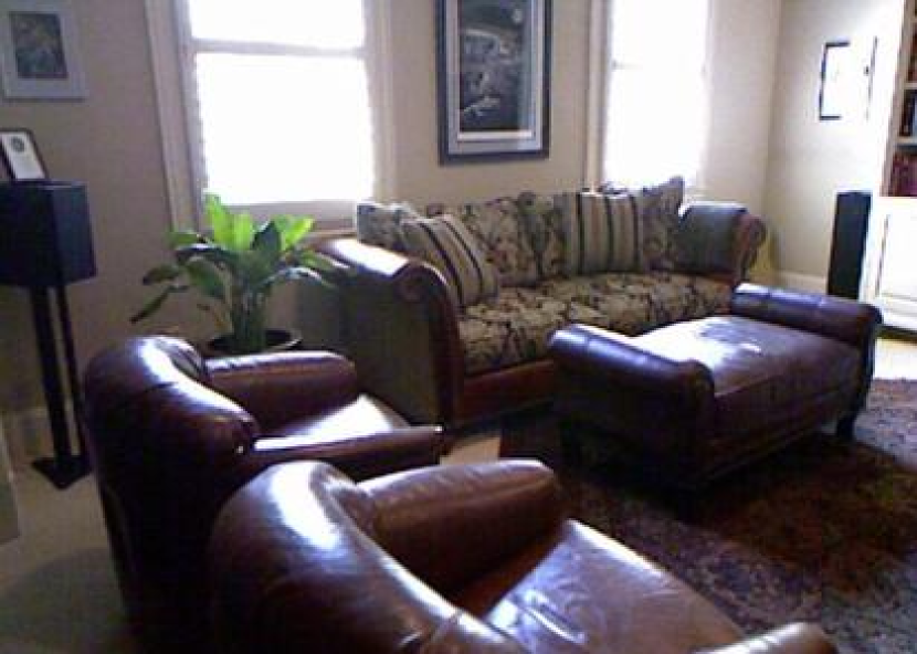
(a) Input image

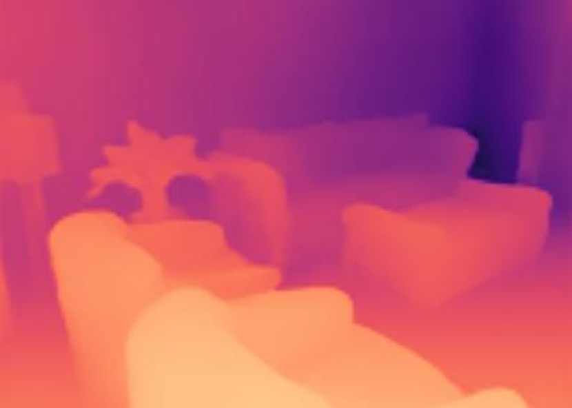
(b) Output depth

(c) Intermediate representations

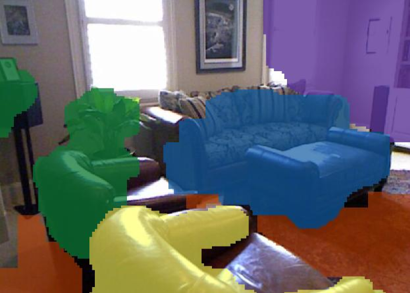
(d) Internal discretization

Figure 1: We propose iDisc which implicitly enforces an internal discretization of the scene via a continuous-discrete-continuous bottleneck. Supervision is applied to the output depth only, i.e., the fused intermediate representations in 1(c), while the internal discrete representations are implicitly learned by the model. 1(d) displays some actual internal discretization patterns captured from the input, e.g., foreground, object relationships, and 3D planes. Our iDisc model is able to predict high-quality depth maps by capturing scene interactions and structure.

Depth estimation is essential in computer vision, especially for understanding geometric relations in a scene. This task consists in predicting the distance between the projection center and the 3D point corresponding to each pixel. Depth estimation finds direct significance in downstream applications such as 3D modeling, robotics, and autonomous cars. Some research [67] shows that depth estimation is a crucial prompt to be leveraged for action reasoning and execution. In particular, we tackle the task of monocular depth estimation (MDE). MDE is an ill-posed problem due to its inherent scale ambiguity: the same 2D input image can correspond to an infinite number of 3D scenes.

State-of-the-art (SotA) methods typically involve convolutional networks [14, 15, 27] or, since the advent of vision Transformer [13], transformer architectures [5, 59, 46, 64]. Most methods either impose geometric constraints on the image [60, 25, 37, 42], namely, planarity priors or explicitly discretize the continuous depth range [15, 5, 6]. The latter can be viewed as learning frontoparallel planes. These imposed priors inherently limit the expressiveness of the respective models, as they cannot model arbitrary depth patterns, ubiquitous in real-world scenes.

We instead propose a more general depth estimation model, called iDisc, which does not explicitly impose any constraint on the final prediction. We design an Internal Discretization (ID) of the scene which is in principle depth-agnostic. Our assumption behind this ID is that each scene can be implicitly described by a set of concepts or patterns, such as objects, planes, edges, and perspectivity relationships. The specific training signal determines which patterns to learn (see Fig. 1).

We design a continuous-to-discrete bottleneck through which the information is passed in order to obtain such internal scene discretization, namely the underlying patterns. In the bottleneck, the scene feature space is partitioned via learnable and input-dependent quantizers, which in turn transfer the information onto the continuous output space. The ID bottleneck introduced in this work is a general concept and can be implemented in several ways. Our particular ID implementation employs attention-based operators, leading to an end-to-end trainable architecture and input-dependent framework. More specifically, we implement the continuous-to-discrete operation via “transposed” cross-attention, where transposed refers to applying $\mathrm{softmax}$ on the output dimension. This $\mathrm{softmax}$ formulation enforces the input features to be routed to the internal discrete representations (IDRs) in an exclusive fashion, thus defining an input-dependent soft clustering of the feature space. The discrete-to-continuous transformation is implemented via cross-attention. Supervision is only applied to the final output, without any assumptions or regularization on the IDRs.

We test iDisc on multiple indoor and outdoor datasets and probe its robustness via zero-shot testing. As of today, there is too little variety in MDE benchmarks for the outdoor scenario, since the only established benchmark is KITTI [19]. Moreover, we observe that all methods fail on outdoor zero-shot testing, suggesting that the KITTI dataset is not diverse enough and leads to overfitting, thus implying that it is not indicative of generalized performance. Hence, we find it compelling to establish a new benchmark setup for the MDE community by proposing two new train-test splits of more diverse and challenging high-quality outdoor datasets: Argoverse1.1 [10] and DDAD [20].

Our main contributions are as follows: (i) we introduce the Internal Discretization module, a novel architectural component that adeptly represents a scene by combining underlying patterns; (ii) we show that it is a generalization of SotA methods involving depth ordinal regression [15, 5]; (iii) we propose splits of two raw outdoor datasets [10, 20] with high-quality LiDAR measurements. We extensively test iDisc on six diverse datasets and, owing to the ID design, our model consistently outperforms SotA methods and presents better transferability. Moreover, we apply iDisc to surface normal estimation showing that the proposed module is general enough to tackle generic real-valued dense prediction tasks.

2 Related Work

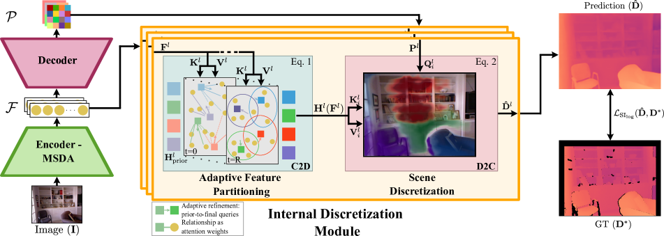
Figure 2: Model Architecture. The Internal Discretization Module imposes an information bottleneck via two consecutive stages: continuous-to-discrete (C2D) and discrete-to-continuous (D2C). The module processes multiple resolutions, i.e., $l\in\{1,2,3\}$, independently in parallel. The bottleneck embodies our assumption that a scene can be represented as a set of patterns. The C2D stage aggregates information, given a learnable prior ($\mathbf{H}^{l}_{\text{prior}}$), from the $l$-th resolution feature maps ($\mathbf{F}^{l}$) to a finite set of IDRs ($\mathbf{H}^{l}$). In particular, it learns how to define a partition function that is dependent on the input $\mathbf{F}^{l}$ via transposed cross-attention, as in (1). The second stage (D2C) transfers the IDRs on the original continuous space using layers of cross-attention as in (2), for sake of simplicity, we depict only a generic $i$-th layer. Cross-attention is guided by the similarity between decoded pixel embeddings ($\mathbf{P}^{l}$) and $\mathbf{H}^{l}$. The final prediction ($\mathbf{\hat{D}}$) is the fusion, i.e., mean, of the intermediate representations $\{\mathbf{\hat{D}}^{l}\}_{l=1}^{3}$.

The supervised setting of MDE assumes that pixel-wise depth annotations are available at training time and depth inference is performed on single images. The coarse-to-fine network introduced in Eigen et al. [14] is the cornerstone in MDE with end-to-end neural networks. The work established the optimization process via the Scale-Invariant log loss ($\mathrm{SI}_{\log}$). Since then, the three main directions evolve: new architectures, such as residual networks [26], neural fields [34, 57], multi-scale fusion [28, 39], transformers [59, 5, 64]; improved optimization schemes, such as reverse-Huber loss [26], classification [8], or ordinal regression [15, 5]; multi-task learning to leverage ancillary information from the related task, such as surface normals estimation or semantic segmentation [14, 43, 56].

Geometric priors have been widely utilized in the literature, particularly the piecewise planarity prior [16, 11, 7], serving as a proper real-world approximation. The geometric priors are usually incorporated by explicitly treating the image as a set of planes [33, 32, 63, 30], using a plane-inducing loss [62], forcing pixels to attend to the planar representation of other pixels [27, 42], or imposing consistency with other tasks’ output [60, 37, 4], like surface normals. Priors can focus on a more holistic scene representation by dividing the whole scene into 3D planes without dependence on intrinsic camera parameters [58, 65], aiming at partitioning the scene into dominant depth planes. In contrast to geometric prior-based works, our method lifts any explicit geometric constraints on the scene. Instead, iDisc implicitly enforces the representation of scenes as a set of high-level patterns.

Ordinal regression methods [15, 5, 6] have proven to be a promising alternative to other geometry-driven approaches. The difference with classification models is that class “values” are learnable and are real numbers, thus the problem falls into the regression category. The typical SotA rationale is to explicitly discretize the continuous output depth range, rendering the approach similar to mask-based segmentation. Each of the scalar depth values is associated with a confidence mask which describes the probability of each pixel presenting such a depth value. Hence, SotA methods inherently assume that depth can be represented as a set of frontoparallel planes, that is, depth “masks”.

The main paradigm of ordinal regression methods is to first obtain hidden representations and scalar values of discrete depth values. The dot-product similarity between the feature maps and the depth representations is treated as logits and $\mathrm{softmax}$ is applied to extract confidence masks (in Fu et al. [15] this degenerates to $\mathrm{argmax}$). Finally, the final prediction is defined as the per-pixel weighted average of the discrete depth values, with the confidence values serving as the weights. iDisc draws connections with the idea of depth discretization. However, our ID module is designed to be depth-agnostic. The discretization occurs at the abstract level of internal features from the ID bottleneck instead of the output depth level, unlike other methods.

Iterative routing is related to our “transposed” cross-attention. The first approach of this kind was Capsule Networks and their variants [47, 23]. Some formulations [51, 36] employ different kinds of attention mechanisms. Our attention mechanism draws connections with [36]. However, we do not allow permutation invariance, since our assumption is that each discrete representation internally describes a particular kind of pattern. In addition, we do not introduce any other architectural components such as gated recurrent units (GRU). In contrast to other methods, our attention is employed at a higher abstraction level, namely in the decoder.

3 Method

We propose an Internal Discretization (ID) module, to discretize the internal feature representation of encoder-decoder network architectures. We hypothesize that the module can break down the scenes into coherent concepts without semantic supervision. This section will first describe the module design and then discuss the network architecture. Sec. 3.1.1 defines the formulation of “transposed” cross-attention outlined in Sec. 1 and describes the main difference with previous formulations from Sec. 2. Moreover, we derive in Sec. 3.1.2 how the iDisc formulation can be interpreted as a generalization of SotA ordinal regression methods by reframing their original formulation. Eventually, Sec. 3.2 presents the optimization problem and the overall architecture.

3.1 Internal Discretization Module

The ID module involves a continuous-discrete-continuous bottleneck composed of two main consecutive stages. The overall module is based on our hypothesis that scenes can be represented as a finite set of patterns. The first stage consists in a continuous-to-discrete component, namely soft-exclusive discretization of the feature space. More specifically, it enforces an input-dependent soft clustering on the feature maps in an image-to-set fashion. The second stage completes the internal scene discretization by mapping the learned IDRs onto the continuous output space. IDRs are not bounded to focus exclusively on depth planes but are allowed to represent any high-level pattern or concept, such as objects, relative locations, and planes in the 3D space. In contrast with SotA ordinal regression methods [15, 5, 6], the IDRs are neither explicitly tied to depth values nor directly tied to the output. Moreover, our module operates at multiple intermediate resolutions and merges them only in the last layer. The overall architecture of iDisc, particularly our ID module, is shown in Fig. 2.

3.1.1 Adaptive Feature Partitioning

The first stage of our ID module, Adaptive Feature Partitioning (AFP), generates proper discrete representations ($\mathcal{H}\coloneqq\{\mathbf{H}^{l}\}^{3}_{l=1}$) that quantize the feature space ($\mathcal{F}\coloneqq\{\mathbf{F}^{l}\}^{3}_{l=1}$) at each resolution $l$. We drop the resolution superscript $l$ since resolutions are independently processed and only one generic resolution is treated here. iDisc does not simply learn fixed centroids, as in standard clustering, but rather learns how to define a partition function in an input-dependent fashion. More specifically, an iterative transposed cross-attention module is utilized. Given the specific input feature maps ($\mathbf{F}$), the iteration process refines (learnable) IDR priors ($\mathbf{H}_{\text{prior}}$) over $R$ iterations.

More specifically, the term “transposed” refers to the different axis along which the $\mathrm{softmax}$ operation is applied, namely $\left[\mathrm{softmax}(\mathbf{K}\mathbf{Q}^{T})\right]^{T}\mathbf{V}$ instead of the canonical dot-product attention $\mathrm{softmax}(\mathbf{Q}\mathbf{K}^{T})\mathbf{V}$, with $\mathbf{Q},\mathbf{K},\mathbf{V}$ as query, key and value tensors, respectively. In particular, the tensors are obtained as projections of feature maps and IDR priors, $f_{\mathbf{Q}}(\mathbf{H}_{\text{prior}})$, $f_{\mathbf{K}}(\mathbf{F})$, $f_{\mathbf{V}}(\mathbf{F})$. The $t$-th iteration out of $R$ can be formulated as follows:

$$W_{ij}^{t}=\frac{\exp(\mathbf{k}_{i}^{T}\mathbf{q}_{j}^{t})}{\sum_{k=1}^{N}\exp(\mathbf{k}_{i}^{T}\mathbf{q}_{k}^{t})},\mathbf{q}_{j}^{t+1}=\sum_{i=1}^{M}W_{ij}^{t}\mathbf{v}_{i},$$ (1)

where $\mathbf{q}_{j},\mathbf{k}_{i},\mathbf{v}_{i}\in\mathbb{R}^{C}$ are query, key and value respectively, $N$ is the number of IDRs, nameley, clusters, and $M$ is the number of pixels. The weights $W_{ij}$ may be normalized to 1 along the $i$ dimension to avoid vanishing or exploding quantities due to the summation of un-normalized distribution.

The quantization stems from the inherent behavior of $\mathrm{softmax}$. In particular, $\mathrm{softmax}$ forces competition among outputs: one output can be large only to the detriment of others. Therefore, when fixing $i$, namely, given a feature, only a few attention weights ($W_{ij}$) may be significantly greater than zero. Hence, the content $\mathbf{v}_{i}$ is routed only to a few IDRs at the successive iteration. Feature maps are fixed during the process and weights are shared by design, thus $\{\mathbf{k}_{i},\mathbf{v}_{i}\}_{i=1}^{M}$ are the same across iterations. The induced competition enforces a soft clustering of the input feature space, where the last-iteration IDR represents the actual partition function ($\mathbf{H}\coloneqq\mathbf{Q}^{R}$). The probabilities of belonging to one partition are the attention weights, namely $W^{R}_{ij}$ with $j$-th query fixed. Since attention weights are inherently dependent on the input, the specific partitioning also depends on the input and takes place at inference time. The entire process of AFP leads to (soft) mutually exclusive IDRs.

As far as the partitioning rationale is concerned, the proposed AFP draws connections with iterative routing methods described in Sec. 2. However, important distinctions apply. First, IDRs are not randomly initialized as the “slots” in Locatello et al. [36] but present a learnable prior. Priors can be seen as learnable positional embeddings in the attention context, thus we do not allow a permutation-invariant set of representations. Moreover, non-adaptive partitioning can still take place via the learnable priors if the iterations are zero. Second, the overall architecture differs noticeably as described in Sec. 2, and in addition, iDisc partitions feature space at the decoder level, corresponding to more abstract, high-level concepts, while the SotA formulations focus on clustering at an abstraction level close to the input image.

One possible alternative approach to obtaining the aforementioned IDRs is the well-known image-to-set proposed in DETR [9], namely via classic cross-attention between representations and image feature maps. However, the corresponding representations might redundantly aggregate features, where the extreme corresponds to each output being the mean of the input. Studies [17, 49] have shown that slow convergence in transformer-based architectures may be due to the non-localized context in cross-attention. The exclusiveness of the IDRs discourages the redundancy of information in different IDRs. We argue that exclusiveness allows the utilization of fewer representations (32 against the 256 utilized in [5] and [15]), and can improve both the interpretability of what IDRs are responsible for and training convergence.

3.1.2 Internal Scene Discretization

In the second stage of the ID module, Internal Scene Discretization (ISD), the module ingests pixel embeddings ($\mathcal{P}\coloneqq\{\mathbf{P}^{l}\}^{3}_{l=1}$) from the decoder and IDRs $\mathcal{H}$ from the first stage, both at different resolutions $l$, as shown in Fig. 2. Each discrete representation carries both the signature, as the key, and the output-related content, as the value, of the pattern it represents. The similarity between IDRs and pixel embeddings is computed in order to spatially localize in the continuous output space where to transfer the information of each IDR. We utilize the dot-product similarity function.

Furthermore, the kind of information to transfer onto the final prediction is not constrained, as we never explicitly handle depth values, usually called bins, until the final output. Thus, the IDRs are completely free to carry generic high-level concepts (such as object-ness, relative positioning, and geometric structures). This approach is in stark contrast with SotA methods [15, 5, 31, 6], which explicitly constrain what the representations are about: scalar depth values. Instead, iDisc learns to generate unconstrained representations in an input-dependent fashion. The effective discretization of the scene occurs in the second stage thanks to the information transfer from the set of exclusive concepts ($\mathcal{H}$) from AFP to the continuous space defined by $\mathcal{P}$. We show that our method is not bounded to depth estimation, but can be applied to generic continuous dense tasks, for instance, surface normal estimation. Consequently, we argue that the training signal of the task at hand determines how to internally discretize the scene, rendering our ID module general and usable in settings other than depth estimation.

From a practical point of view, the whole second stage consists in cross-attention layers applied to IDRs and pixel embeddings. As described in Sec. 3.1.1, we drop the resolution superscript $l$. After that, the final depth maps are projected onto the output space and the multi-resolution depth predictions are combined. The $i$-th layer is defined as:

$$\mathbf{D}_{i+1}=\mathrm{softmax}(\mathbf{Q}_{i}\mathbf{K}_{i}^{T})\mathbf{V}_{i}+\mathbf{D}_{i},$$ (2)

where $\mathbf{Q}_{i}=f_{Q_{i}}(\mathbf{P})\in\mathbb{R}^{H\times{}W\times{}C}$, $\mathbf{P}$ are pixel embeddings with shape $(H,W)$, and $\mathbf{K}_{i},\mathbf{V}_{i}\in\mathbb{R}^{N\times C}$ are the $N$ IDRs under linear transformations $f_{K_{i}}(\mathbf{H})$, $f_{V_{i}}(\mathbf{H})$. The term $\mathbf{Q}_{i}\mathbf{K}_{i}^{T}$ determines the spatial location for which each specific IDR is responsible, while $\mathbf{V}_{i}$ carries the semantic content to be transferred in the proper spatial locations.

Our approach constitutes a generalization of depth estimation methods that involve (hybrid) ordinal regression. As described in Sec. 2, the common paradigm in ordinal regression methods is to explicitly discretize depth in a set of masks with a scalar depth value associated with it. Then, they predict the likelihood that each pixel belongs to such masks. Our change of paradigm stems from the reinterpretation of the mentioned ordinal regression pipeline which we translate into the following mathematical expression:

$$\mathbf{D}=\mathrm{softmax}(\mathbf{P}\mathbf{R}^{T}\mathbin{/}T)\mathbf{v},$$ (3)

where $\mathbf{P}$ are the pixel embeddings at maximum resolution and $T$ is the $\mathrm{softmax}$ temperature. $\mathbf{v}\in\mathbb{R}^{N\times 1}$ are $N$ depth scalar values and $\mathbf{R}\in\mathbb{R}^{N\times(C-1)}$ are their hidden representations, both processed as a unique stacked tensor ($\mathbf{R}||\mathbf{v}\in\mathbb{R}^{N\times C}$). From the reformulation in (3), one can observe that (3) is a degenerate case of (2). In particular, $f_{Q}$ degenerates to the identity function. $f_{K}$ and $f_{V}$ degenerate to selector functions: the former function selects up to the $C-1$ dimensions and the latter selects the last dimension only. Moreover, the hidden representations are refined pixel embeddings ($f(\mathbf{P}_{i})=\mathbf{H}_{i}=\mathbf{R}||\mathbf{v}$), and $\mathbf{D}$ in (3) is the final output, namely no multiple iterations are performed as in (2). The explicit entanglement between the semantic content of the hidden representations and the final output is due to hard-coding $\mathbf{v}$ as depth scalar values.

3.2 Network Architecture

Our network described in Fig. 2 comprises first an encoder backbone, interchangeably convolutional or attention-based, producing features at different scales. The encoded features at different resolutions are refined, and information between resolutions is shared, both via four multi-scale deformable attention (MSDA) blocks [68]. The feature maps from MSDA at different scales are fed into the AFP module to extract IDRs ($\mathcal{H}$), and into the decoder to extract pixel embeddings in the continuous space ($\mathcal{P}$). Pixel embeddings at different resolutions are combined with the respective IDRs in the ISD stage of the ID module to extract the depth maps. The final depth prediction corresponds to the mean of the interpolated intermediate representations. The optimization process is guided only by the established $\mathrm{SI_{log}}$ loss defined in [14], and no other regularization is exploited. $\mathrm{SI_{log}}$ is defined as:

$$\begin{split}&\mathcal{L}_{\mathrm{SI_{log}}}(\epsilon)=\alpha\sqrt{\mathbb{V}[\epsilon]+\lambda\mathbb{E}^{2}[\epsilon]}\\ &\text{with }\epsilon=\log(\hat{y})-\log(y^{*}),\end{split}$$ (4)

where $\hat{y}$ is the predicted depth and $y^{*}$ is the ground-truth (GT) value. $\mathbb{V}[\epsilon]$ and $\mathbb{E}[\epsilon]$ are computed as the empirical variance and expected value over all pixels, namely, $\{\epsilon_{i}\}_{i=1}^{N}$. $\mathbb{V}[\epsilon]$ is the purely scale-invariant loss, while $\mathbb{E}^{2}[\epsilon]$ fosters a proper scale. $\alpha$ and $\lambda$ are set to $10$ and $0.15$, as customary.

4 Experiments

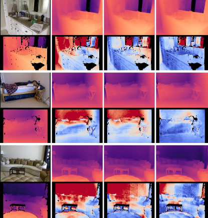
Image+GT        AdaBins[5]     NeWCRF[64]         Ours

Figure 3: Qualitative results on NYU. Each pair of consecutive rows corresponds to one test sample. Each odd row shows the input RGB image and depth predictions for the selected methods. Each even row shows GT depth and the prediction errors of the selected methods clipped at 0.5 meters. The error color map is coolwarm: blue corresponds to lower error values and red to higher values.

4.1 Experimental Setup

4.1.1 Datasets

NYU-Depth V2. NYU-Depth V2 (NYU) [40] is a dataset consisting of 464 indoor scenes with RGB images and quasi-dense depth images with 640$\times{}$480 resolution. Our models are trained on the train-test split proposed by previous methods [27], corresponding to 24,231 samples for training and 654 for testing. In addition to depth, the dataset provides surface normal data utilized for normal estimation. The train split used for normal estimation is the one proposed in [60].

Zero-shot testing datasets. We evaluate the generalizability of indoor models on two indoor datasets which are not seen during training. The selected datasets are SUN-RGBD [48] and DIODE-Indoor [52]. For both datasets, the resolution is reduced to match that of NYU, which is 640$\times{}$480.

KITTI. The KITTI dataset provides stereo images and corresponding Velodyne LiDAR scans of outdoor scenes captured from a moving vehicle [19]. RGB and depth images have (mean) resolution of 1241$\times{}$376. The split proposed by [14] (Eigen-split) with corrected depth is utilized as training and testing set, namely, 23,158 and 652 samples. The evaluation crop corresponds to the crop defined by [18]. All methods in Sec. 4.2 that have source code and pre-trained models available are re-evaluated on KITTI with the evaluation mask from [18] to have consistent results.

Argoverse1.1 and DDAD. We propose splits of two autonomous driving datasets, Argoverse1.1 (Argoverse) [10] and DDAD [20], for depth estimation. Argoverse and DDAD are both outdoor datasets that provide 360^∘ HD images and the corresponding LiDAR scans from moving vehicles. We pre-process the original datasets to extract depth maps and avoid redundancy. Training set scenes are sampled when the vehicle has been displaced by at least 2 meters from the previous sample. For the testing set scenes, we increase this threshold to 50 meters to further diminish redundancy. Our Argoverse split accounts for 21,672 training samples and 476 test samples, while DDAD for 18,380 training and 860 testing samples. Samples in Argoverse are taken from the 6 cameras covering the full 360^∘ panorama. For DDAD, we exclude 2 out of the 6 cameras since they have more than 30% pixels occluded by the camera capture system. We crop both RGB images and depth maps to have 1920$\times$870 resolution that is 180px and 210px cropped from the top for Argoverse and DDAD, respectively, to crop out a large portion of the sky and regions occluded by the ego-vehicle. For both datasets, we clip the maximum depth at 150m.

4.1.2 Implementation Details

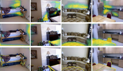
Figure 4: Attention maps on NYU for three different IDRs. Each row presents the attention map of a specific IDR for four test images. Each discrete representation focuses on a specific high-level concept. The first two rows pertain to IDRs at the lowest resolution while the last corresponds to the highest resolution. Best viewed on a screen and zoomed in.

Evaluation Details. In all experiments, we do not exploit any test-time augmentations (TTA), camera parameters, or other tricks and regularizations, in contrast to many previous methods [15, 27, 5, 42, 64]. This provides a more challenging setup, which allows us to show the effectiveness of iDisc. As depth estimation metrics, we utilize root mean square error ($\mathrm{RMS}$) and its log variant ($\mathrm{RMS_{log}}$), absolute error in log-scale ($\mathrm{Log_{10}}$), absolute ($\mathrm{A.Rel}$) and squared ($\mathrm{S.rel}$) mean relative error, the percentage of inlier pixels ($\mathrm{\delta}_{i}$) with threshold $1.25^{i}$, and scale-invariant error in log-scale ($\mathrm{SI_{log}}$): $100\sqrt{\mathrm{Var}(\epsilon_{\log})}$. The maximum depth for NYU and all zero-shot testing in indoor datasets, specifically SUN-RGBD and Diode Indoor, is set to 10m, while for KITTI it is set to 80m and for Argoverse and DDAD to 150m. Zero-shot testing is performed by evaluating a model trained on either KITTI or NYU and tested on either outdoor or indoor datasets, respectively, without additional fine-tuning. For surface normals estimation, the metrics are mean ($\mathrm{Mean}$) and median ($\mathrm{Med}$) absolute error, $\mathrm{RMS}$ angular error, and percentages of inlier pixels with thresholds at $11.5^{\circ}$, $22.5^{\circ}$, and $30^{\circ}$. GT-based mean depth rescaling is applied only on Diode Indoor for all methods since the dataset presents largely scale-equivariant scenes, such as plain walls with tiny details.

Training Details. We implement iDisc in PyTorch [41]. For training, we use the AdamW [38] optimizer ($\beta_{1}=0.9$, $\beta_{2}=0.999$) with an initial learning rate of $0.0002$ for every experiment, and weight decay set to $0.02$. As a scheduler, we exploit Cosine Annealing starting from 30% of the training, with final learning rate of $0.00002$. We run 45k optimization iterations with a batch size of 16. All backbones are initialized with weights from ImageNet-pretrained models. The augmentations include both geometric (random rotation and scale) and appearance (random brightness, gamma, saturation, hue shift) augmentations. The required training time amounts to 20 hours on 4 NVidia Titan RTX.

4.2 Comparison with the State of the Art

Table 1: Comparison on NYU official test set. R101: ResNet-101 [21], D161: DenseNet-161 [24], EB5: EfficientNet-B5 [50], HR48: HRNet-48 [53], DD22: DRN-D-22 [61], ViTB: ViT-B/16+Resnet-50 [13], MViT: EfficientNet-B5-AP [55]+MiniViT, Swin{L, B, T}: Swin-{Large, Base, Tiny} [35]. (†): ImageNet-22k [12] pretraining, (‡): non-standard training set, ($\ast$): in-house dataset pretraining, (§): re-evaluated without GT-based rescaling.

Method	Encoder	$\boldsymbol{\delta_{1}}$	$\boldsymbol{\delta_{2}}$	$\boldsymbol{\delta_{3}}$	$\mathbf{RMS}$	$\mathbf{A.Rel}$	$\mathbf{Log_{10}}$
		Higher is better			Lower is better
Eigen et al. [14]	-	$0.769$	$0.950$	$0.988$	$0.641$	$0.158$	$-$
DORN [15]	R101	$0.828$	$0.965$	$0.992$	$0.509$	$0.115$	$0.051$
VNL [60]	-	$0.875$	$0.976$	$0.994$	$0.416$	$0.108$	$0.048$
BTS [27]	D161	$0.885$	$0.978$	$0.994$	$0.392$	$0.110$	$0.047$
AdaBins‡ [5]	MViT	$0.903$	$0.984$	$0.997$	$0.364$	$0.103$	$0.044$
DAV [25]	DD22	$0.882$	$0.980$	$0.996$	$0.412$	$0.108$	$-$
Long et al. [37]	HR48	$0.890$	$0.982$	$0.996$	$0.377$	$0.101$	$0.044$
TransDepth [59]	ViTB	$0.900$	$0.983$	$0.996$	$0.365$	$0.106$	$0.045$
DPT*[46]	ViTB	$0.904$	$0.988$	$0.998$	$0.357$	$0.110$	$0.045$
P3Depth§ [42]	R101	$0.830$	$0.971$	$0.995$	$0.450$	$0.130$	$0.056$
NeWCRF [64]	SwinL†	$0.922$	$0.992$	$0.998$	$0.334$	$0.095$	$0.041$
LocalBins‡ [6]	MViT	$0.907$	$0.987$	$0.998$	$0.357$	$0.099$	$0.042$
Ours	R101	$0.892$	$0.983$	$0.995$	$0.380$	$0.109$	$0.046$
	EB5	$0.903$	$0.986$	$0.997$	$0.369$	$0.104$	$0.044$
	SwinT	$0.894$	$0.983$	$0.996$	$0.377$	$0.109$	$0.045$
	SwinB	$0.926$	$0.989$	$0.997$	$0.327$	$0.091$	$0.039$
	SwinL†	$\mathbf{0.940}$	$\mathbf{0.993}$	$\mathbf{0.999}$	$\mathbf{0.313}$	$\mathbf{0.086}$	$\mathbf{0.037}$

Indoor Datasets. Results on NYU are presented in Table 1. The results show that we set the new state of the art on the benchmark, improving by more than 6% on $\mathrm{RMS}$ and 9% on $\mathrm{A.Rel}$ over the previous SotA. Moreover, results highlight how iDisc is more sample-efficient than other transformer-based architectures [46, 59, 5, 64, 6] since we achieve better results even when employing smaller and less heavily pre-trained backbone architectures. In addition, results show a significant improvement in performance with our model instantiated with a full-convolutional backbone over other full-convolutional-based models [14, 15, 27, 25, 42]. Table 2 presents zero-shot testing of NYU models on SUN-RGBD and Diode. In both cases, iDisc exhibits a compelling generalization performance, which we argue is due to implicitly learning the underlying patterns, namely, IDRs, of indoor scene structure via the ID module.

Table 2: Zero-shot testing of models trained on NYU. All methods are trained on NYU and tested without further fine-tuning on the official validation set of SUN-RGBD and Diode Indoor.

Test set	Method	$\boldsymbol{\delta_{1}}\uparrow$	$\mathbf{RMS}\downarrow$	$\mathbf{A.Rel}\downarrow$	$\mathbf{SI_{log}}\downarrow$
SUN-RGBD	BTS [27]	$0.745$	$0.502$	$0.168$	$14.25$
	AdaBins [5]	$0.768$	$0.476$	$0.155$	$13.20$
	P3Depth [42]	$0.698$	$0.541$	$0.178$	$15.02$
	NeWCRF [64]	$0.799$	$0.429$	$0.150$	$11.27$
	Ours	$\mathbf{0.838}$	$\mathbf{0.387}$	$\mathbf{0.128}$	$\mathbf{10.91}$
Diode	BTS [27]	$0.705$	$0.965$	$0.211$	$23.78$
	AdaBins [5]	$0.733$	$0.872$	$0.209$	$22.54$
	P3Depth [42]	$0.732$	$0.877$	$0.202$	$22.16$
	NeWCRF [64]	$0.799$	$0.769$	$0.164$	$18.69$
	Ours	$\mathbf{0.810}$	$\mathbf{0.721}$	$\mathbf{0.156}$	$\mathbf{18.11}$

Qualitative results in Fig. 3 emphasize how the method excels in capturing the overall scene complexity. In particular, iDisc correctly captures discontinuities without depth over-excitation due to chromatic edges, such as the sink in row 1, and captures the right perspectivity between foreground and background depth planes such as between the bed (row 2) or sofa (row 3) and the walls behind. In addition, the model presents a reduced error around edges, even when compared to higher-resolution models such as [5]. We argue that iDisc actually reasons at the pattern level, thus capturing better the structure of the scene. This is particularly appreciable in indoor scenes, since these are usually populated by a multitude of objects. This behavior is displayed in the attention maps of Fig. 4. Fig. 4 shows how IDRs at lower resolution capture specific components, such as the relative position of the background (row 1) and foreground objects (row 2), while IDRs at higher resolution behave as depth refiners, attending typically to high-frequency features, such as upper (row 3) or lower borders of objects. It is worth noting that an IDR attends to the image borders when the particular concept it looks for is not present in the image. That is, the borders are the last resort in which the IDR tries to find its corresponding pattern (e.g., row 2, col. 1).

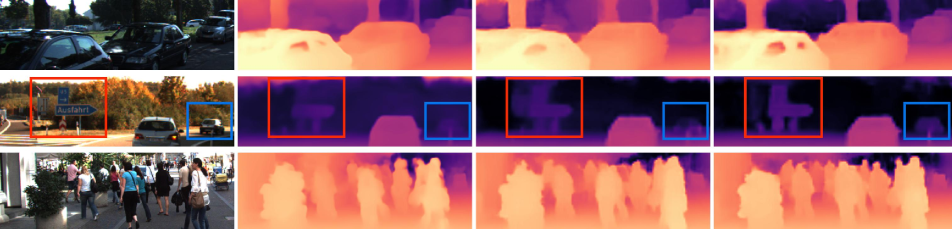
Image                                      AdaBins[5]                              NeWCRF[64]                                  Ours

Figure 5: Qualitative results on KITTI. Three zoomed-in crops of different test images are shown. The comparisons show the ability of iDisc to capture small details, proper background transition, and fine-grained variations in, e.g., crowded scenes. Best viewed on a screen.

Table 3: Comparison on KITTI Eigen-split test set. Models without $\delta_{0.5}$ have implementation (partially) unavailable. R101: ResNet-101 [21], D161: DenseNet-161 [24], EB5: EfficientNet-B5[50], ViTB: ViT-B/16+Resnet-50 [13], MViT: EfficientNet-B5-AP [55]+MiniViT, Swin{L, B, T}: Swin-{Large, Base, Tiny} [35]. (†): ImageNet-22k [12] pretraining, (‡): non-standard training set, ($\ast$): in-house dataset pretraining, (§): re-evaluated without GT-based rescaling.

Method	Encoder	$\boldsymbol{\delta_{0.5}}$	$\boldsymbol{\delta_{1}}$	$\boldsymbol{\delta_{2}}$	$\mathbf{RMS}$	$\mathbf{RMS_{log}}$	$\mathbf{A.Rel}$	$\mathbf{S.Rel}$
		Higher is better			Lower is better
Eigenet al. [14]	$-$	$-$	$0.692$	$0.899$	$7.156$	$0.270$	$0.190$	$1.515$
DORN [15]	R101	$-$	$0.932$	$0.984$	$2.727$	$0.120$	$0.072$	$0.307$
BTS [27]	D161	$0.870$	$0.964$	$0.995$	$2.459$	$0.090$	$0.057$	$0.199$
AdaBins‡ [5]	MViT	$0.868$	$0.964$	$0.995$	$2.360$	$0.088$	$0.058$	$0.198$
TransDepth [59]	ViTB	$-$	$0.956$	$0.994$	$2.755$	$0.098$	$0.064$	$0.252$
DPT* [46]	ViTB	$0.865$	$0.965$	$0.996$	$2.315$	$0.088$	$0.059$	$0.190$
P3Depth§ [42]	R101	$0.852$	$0.959$	$0.994$	$2.519$	$0.095$	$0.060$	$0.206$
NeWCRF [64]	SwinL†	$0.887$	$0.974$	$\mathbf{0.997}$	$2.129$	$0.079$	$0.052$	$0.155$
Ours	R101	$0.860$	$0.965$	$0.996$	$2.362$	$0.090$	$0.059$	$0.197$
	EB5	$0.852$	$0.963$	$0.994$	$2.510$	$0.094$	$0.063$	$0.223$
	SwinT	$0.870$	$0.968$	$0.996$	$2.291$	$0.087$	$0.058$	$0.184$
	SwinB	$0.885$	$0.974$	$\mathbf{0.997}$	$2.149$	$0.081$	$0.054$	$0.159$
	SwinL†	$\mathbf{0.896}$	$\mathbf{0.977}$	$\mathbf{0.997}$	$\mathbf{2.067}$	$\mathbf{0.077}$	$\mathbf{0.050}$	$\mathbf{0.145}$

Outdoor Datasets. Results on KITTI in Table 3 demonstrate that iDisc sets the new SotA for this primary outdoor dataset, improving by more than 3% in $\mathrm{RMS}$ and by 0.9% in $\mathrm{\delta_{0.5}}$ over the previous SotA. However, KITTI results present saturated metrics. For instance, $\mathrm{\delta_{3}}$ is not reported since every method scores $>0.99$, with recent ones scoring $0.999$. Therefore, we propose to utilize the metric $\mathrm{\delta_{0.5}}$, to better convey meaningful evaluation information. In addition, iDisc performs remarkably well on the highly competitive official KITTI benchmark, ranking 3^rd among all methods and 1^st among all published MDE methods.

Moreover, Table 4 shows the results of methods trained and evaluated on the splits from Argoverse and DDAD proposed in this work. All methods have been trained with the same architecture and pipeline utilized for training on KITTI. We argue that the high degree of sparseness in GT of the two proposed datasets, in contrast to KITTI, deeply affects windowed methods such as [5, 64]. Qualitative results in Fig. 5 suggest that the scene level discretization leads to retaining small objects and sharp transitions between foreground objects and background: background in row 1, and boxes in row 2. These results show the better ability of iDisc to capture fine-grained depth variations on close-by and similar objects, including crowd in row 3. Zero-shot testing from KITTI to DDAD and Argoverse are presented in Supplement.

Table 4: Comparison on Argoverse and DDAD proposed splits. Comparison of performance of methods trained on either Argoverse or DDAD and tested on the same dataset.

Dataset	Method	$\boldsymbol{\delta_{1}}$	$\boldsymbol{\delta_{2}}$	$\boldsymbol{\delta_{3}}$	$\mathbf{RMS}$	$\mathbf{RMS_{log}}$	$\mathbf{A.Rel}$	$\mathbf{S.Rel}$
		Higher is better			Lower is better
Argoverse	BTS [27]	$0.780$	$0.908$	$0.954$	$8.319$	$0.267$	$0.186$	$2.56$
	AdaBins [5]	$0.750$	$0.901$	$0.952$	$8.686$	$0.278$	$0.195$	$2.36$
	NeWCRF [64]	$0.707$	$0.871$	$0.939$	$9.437$	$0.321$	$0.232$	$3.23$
	Ours	$\mathbf{0.821}$	$\mathbf{0.923}$	$\mathbf{0.960}$	$\mathbf{7.567}$	$\mathbf{0.243}$	$\mathbf{0.163}$	$\mathbf{2.22}$
DDAD	BTS [27]	$0.757$	$0.913$	$0.962$	$10.11$	$0.251$	$0.186$	$2.27$
	AdaBins [5]	$0.748$	$0.912$	$0.962$	$10.24$	$0.255$	$0.201$	$2.30$
	NeWCRF [64]	$0.702$	$0.881$	$0.951$	$10.98$	$0.271$	$0.219$	$2.83$
	Ours	$\mathbf{0.809}$	$\mathbf{0.934}$	$\mathbf{0.971}$	$\mathbf{8.989}$	$\mathbf{0.221}$	$\mathbf{0.163}$	$\mathbf{1.85}$

Surface Normals Estimation. We emphasize that the proposed method has more general applications by testing iDisc on a different continuous dense prediction task such as surface normals estimation. Results in Table 5 evidence that we set the new state of the art on surface normals estimation. It is worth mentioning that all other methods are specifically designed for normals estimation, while we keep the same architecture and framework from indoor depth estimation.

Table 5: Comparison of surface normals estimation methods on NYU official test set. iDisc architecture and training pipeline is the same as the one utilized for indoor depth estimation.

Method	$\boldsymbol{11.5^{\circ}}$	$\boldsymbol{22.5^{\circ}}$	$\boldsymbol{30^{\circ}}$	$\mathbf{RMS}$	$\mathbf{Mean}$	$\mathbf{Med}$
	Higher is better			Lower is better
SURGE [54]	$0.473$	$0.689$	$0.766$	$-$	$20.6$	$12.2$
GeoNet [43]	$0.484$	$0.484$	$0.795$	$26.9$	$19.0$	$11.8$
PAP [66]	$0.488$	$0.722$	$0.798$	$25.5$	$18.6$	$11.7$
GeoNet++ [44]	$0.502$	$0.732$	$0.807$	$26.7$	$18.5$	$11.2$
Bae et al. [3]	$0.622$	$0.793$	$0.852$	$23.5$	$14.9$	$7.5$
Ours	$\mathbf{0.638}$	$\mathbf{0.798}$	$\mathbf{0.856}$	$\mathbf{22.8}$	$\mathbf{14.6}$	$\mathbf{7.3}$

4.3 Ablation study

The importance of each component introduced in iDisc is evaluated by ablating the method in Table 6.

Depth Discretization. Internal scene discretization provides a clear improvement over its explicit counterpart (row 3 vs. 2), which is already beneficial in terms of robustness. Adding the MSDA module on top of explicit discretization (row 5) recovers part of the performance gap between the latter and our full method (row 8). We argue that MSDA recovers a better scene scale by refining feature maps at different scales at once, which is helpful for higher-resolution feature maps.

Component Interactions. Using either the MSDA module or the AFP module together with internal scene discretization results in similar performance (rows 4 and 6). We argue that the two modules are complementary, and they synergize when combined (row 8). The complementarity can be explained as follows: in the former scenario (row 4), MSDA preemptively refines feature maps to be partitioned by the non-adaptive clustering, that is, by the IDR priors described in Sec. 3, while on latter one (row 6), AFP allows the IDRs to adapt themselves to partition the unrefined feature space properly. Row 7 shows that the architecture closer to the one in [36], particularly random initialization, hurts performance since the internal representations do not embody any domain-specific prior information.

Table 6: Ablation of iDisc. EDD: Explicit Depth Discretization [15, 5], ISD: Internal Scene discretization, AFP: Adaptive Feature Partitioning, MSDA: MultiScale Deformable Attention. The EDD module, used in SotA methods, and our ISD module are mutually exclusive. AFP with (✓${}_{\textbf{R}}$) refers to random initialization of IDRs and architecture similar to [36]. The last row corresponds to our complete iDisc model.

	EDD	ISD	AFP	MSDA	$\boldsymbol{\delta_{1}}\uparrow$	$\mathbf{RMS}\downarrow$	$\mathbf{A.Rel}\downarrow$
1	✗	✗	✗	✗	$0.890$	$0.370$	$0.104$
2	✓	✗	✗	✗	$0.905$	$0.367$	$0.102$
3	✗	✓	✗	✗	$0.919$	$0.340$	$0.096$
4	✗	✓	✓	✗	$0.931$	$0.319$	$0.091$
5	✓	✗	✗	✓	$0.931$	$0.326$	$0.091$
6	✗	✓	✗	✓	$0.934$	$0.319$	$0.088$
7	✗	✓	✓${}_{\textbf{R}}$	✓	$0.930$	$0.319$	$0.089$
8	✗	✓	✓	✓	$0.940$	$0.313$	$0.086$

5 Conclusion

We have introduced a new module, called Internal Discretization, for MDE. The module represents the assumption that scenes can be represented as a finite set of patterns. Hence, iDisc leverages an internally discretized representation of the scene that is enforced via a continuous-discrete-continuous bottleneck, namely ID module. We have validated the proposed method, without any TTA or tricks, on the primary indoor and outdoor benchmarks for MDE, and have set the new state of the art among supervised approaches. Results showed that learning the underlying patterns, while not imposing any explicit constraints or regularization on the output, is beneficial for performance and generalization. iDisc also works out-of-the-box for normal estimation, beating all specialized SotA methods. In addition, we propose two new challenging outdoor dataset splits, aiming to benefit the community with more general and diverse benchmarks.

Acknowledgment. This work is funded by Toyota Motor Europe via the research project TRACE-Zürich.

Appendix

Appendix A Results

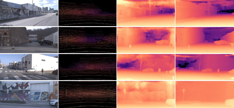
Image                                         GT                                Ours (w/ zero-shot)                                Ours

Figure 16: Qualitative results on Argoverse. Each row corresponds to one zero-shot test sample from Argoverse. The third column displays the prediction of iDisc trained on KITTI and tested on Argoverse, while the fourth column corresponds to a model trained and tested on Argoverse.

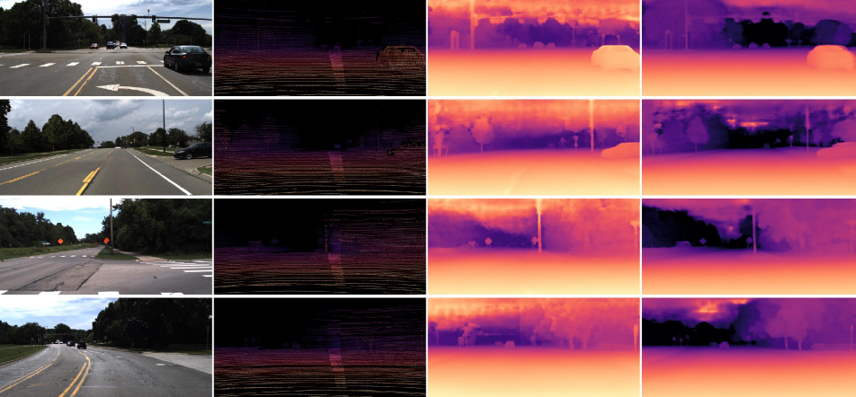
Image                                         GT                                  Ours (zero-shot)                              Ours (sup.)

Figure 17: Qualitative results on DDAD. Each row corresponds to one zero-shot test sample from DDAD. The third column displays the prediction of iDisc trained on KITTI and tested on DDAD, while the fourth corresponds column to a model trained and tested on DDAD.

Outdoor zero-shot. We present in Table 7 the results of models pre-trained on KITTI Eigen-split [14] and tested on Argoverse [10] and DDAD [20] test split we proposed in this work. The zero-shot results clearly demonstrate how every model tends to perform poorly when trained on KITTI and tested on a different domain. However, iDisc is able to almost double the performance when directly trained on either Argoverse or DDAD. This suggests that KITTI is not indicative of generalization performance. This investigation leads us to realize the need for more diversity in the outdoor scenario. We address the problem by proposing new dataset splits to train and validate models on. Fig. 16 shows how models fail completely when predicting unseen scenario, e.g., graffiti on a flat wall. In addition, Fig. 17 displays how models under-scale depth when testing on domains with a typical object size, i.e., DDAD in the United States, larger than that of the training set, i.e., KITTI in Germany.

Table 7: Zero-shot testing of models trained on KITTI Eigen-split. Comparison of performance when methods are trained on KITTI Eigen-split and tested, without further fine-tuning, on the splits of Argoverse and DDAD introduced in this work.

Test set	Method	$\boldsymbol{\delta_{1}}\uparrow$	$\mathbf{RMS}\downarrow$	$\mathbf{A.Rel}\downarrow$	$\mathbf{SI_{log}}\downarrow$
Argoverse	BTS [27]	$0.307$	$15.98$	$0.383$	$51.80$
	AdaBins [5]	$0.383$	$17.07$	$0.350$	$52.33$
	P3Depth [42]	$0.277$	$17.97$	$0.376$	$44.09$
	NeWCRF [64]	$0.311$	$15.75$	$0.370$	$46.77$
	Ours	$\mathbf{0.560}$	$\mathbf{12.18}$	$\mathbf{0.269}$	$\mathbf{33.35}$
DDAD	BTS [27]	$\mathbf{0.399}$	$16.19$	$0.350$	$40.51$
	AdaBins [5]	$0.282$	$18.36$	$0.433$	$50.71$
	P3Depth [42]	$0.397$	$17.83$	$\mathbf{0.330}$	$39.00$
	NeWCRF [64]	$0.343$	$16.76$	$0.375$	$44.24$
	Ours	$0.350$	$\mathbf{14.26}$	$0.367$	$\mathbf{29.37}$

KITTI [19] benchmark. Table 8 clearly shows the compelling performance of iDisc on the official KITTI private test set. We show the results of the latest published methods only. The table is from the official KITTI leaderboard.

Table 8: Results on official KITTI [19] Benchmark. Comparison of performance of methods trained on KITTI and tested on the official KITTI private test set.

Method	$\mathbf{SI_{\log}}$	$\mathbf{Sq.Rel}$	$\mathbf{A.Rel}$	$\mathbf{iRMS}$
	Lower is better
PAP [66]	13.08	2.72 %	10.27 %	13.95
P3Depth [42]	12.82	2.53 %	9.92 %	13.71
VNL [60]	12.65	2.46 %	10.15 %	13.02
DORN [63]	11.77	2.23 %	8.78 %	12.98
BTS [27]	11.67	2.21 %	9.04 %	12.23
PWA [29]	11.45	2.30 %	9.05 %	12.32
ViP-DeepLab [45]	10.80	2.19 %	8.94 %	11.77
NeWCRF [64]	10.39	1.83 %	8.37 %	11.03
PixelFormer [1]	10.28	1.82 %	8.16 %	10.84
Ours (iDisc)	9.89	1.77 %	8.11 %	10.73

Table 9: Comparison on NYU with 3D metrics. F1-score for varying threshold (m) and Chamfer distance (m) on point clouds.

Method	$\mathbf{F1}_{0.05}\uparrow$	$\mathbf{F1}_{0.1}\uparrow$	$\mathbf{F1}_{0.2}\uparrow$	$\mathbf{F1}_{0.3}\uparrow$	$\mathbf{F1}_{0.5}\uparrow$	$\mathbf{F1}_{0.75}\uparrow$	$\mathbf{D}_{\mathrm{Chamfer}}\downarrow$
BTS [27]	$24.5$	$47.0$	$72.4$	$84.4$	$93.6$	$97.2$	$0.169$
AdaBins [5]	$24.0$	$47.0$	$73.0$	$84.7$	$94.0$	$97.4$	$0.163$
NeWCRF [64]	$25.5$	$48.6$	$74.0$	$85.4$	$94.4$	$97.6$	$0.156$
iDisc	$\mathbf{27.8}$	$\mathbf{52.0}$	$\mathbf{77.0}$	$\mathbf{87.8}$	$\mathbf{95.5}$	$\mathbf{98.1}$	$\mathbf{0.131}$

IDRs collapse. We argue that our model is able to avoid over-clustering when performing the adaptive partitioning in AFP step. Over-clustering is the phenomenon occurring when the number of partitions enforced is more than the underlying true one. The ID module is able to avoid over-clustering by degenerating some IDRs onto others, thus not introducing any detrimental partition of the feature space. Degeneration of the same IDR is visible in Fig. 6.

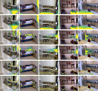
Figure 6: Examples of attention maps degeneration. Each pair of rows shows two different IDRs’ attention maps, each pair is extracted from a different resolution. Some IDRs degenerate onto other IDRs, avoiding over-partitioning when more IDRs than those needed are utilized to represent the scene.

Attention depth planes. Fig. 7 shows three IDRs (each row shows a specific IDR, as in main paper figures) at the middle resolution. The top two rows support the “speculation” on iDisc’s ability to still capture depth planes.

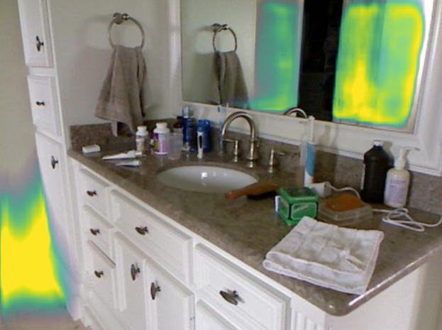
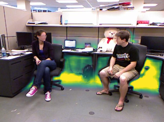
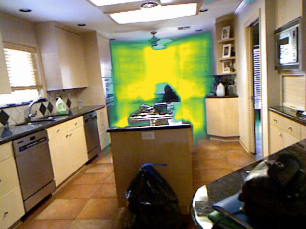
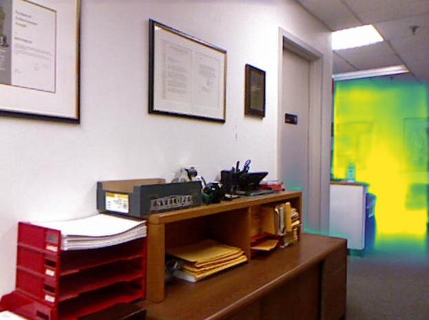
Figure 7: Attention visualization. Attention maps of three different IDRs at mid-resolution, on four different images from NYU.

Computational complexity. We provide the analysis of the components in Table 10. Removing MSDA increases throughput to $20$fps, with only a slight loss in performance. Note that our implementation is not fully optimized for performance. NeWCRF [64] uses the same backbone but more parameters and similar throughput to iDisc without MSDA.

Table 10: Computational complexity analysis on an RTX 3090 with input images of size 640$\times$480 and SWin-L backbone.

Component	Latency (ms)	Throughput (fps)	Parameters (M)
Encoder	$23.6$	$42.4$	$194.9$
MSDA	$72.8$	$13.7$	$2.83$
FPN	$2.7$	$370.5$	$4.11$
AFP	$12.4$	$80.7$	$2.78$
ISD	$9.6$	$103.7$	$4.59$
iDisc (w/o MSDA)	$48.2$	$20.7$	$206.4$
iDisc	$121.1$	$8.3$	$209.2$

Appendix B Ablations

Number of IDRs. We ablate the model with respect to the number of IDRs exploited by iDisc. In particular, we sweep the number of IDRs between 2 and 128 with a base-two log scale. The black-solid line in Fig. 8 shows the trend of iDisc when ablating the IDRs: the optimum is reached in the interval [8, 32]. When more representations are utilized, we argue that noise is introduced in the bottleneck and the discretization process is not actually enforced. The discretization does not occur since the number of IDRs would be close to the number of feature map elements. On the other hand, 2 or 4 IDRs are already enough to obtain decent results, although not particularly visually appealing. In particular, we speculate that the extreme case of utilizing two IDRs can lead to the model representing the maximum depth with one of the two representations and the minimum one with the other. Therefore, the model is still able to interpolate between the depth interval range. The interpolation occurs thanks to the convex combination, defined by $\mathrm{softmax}$, of maximum and minimum depth. More specifically, $\mathrm{softmax}$ is guided by the similarity between the pixel embeddings and the corresponding depth representations. Thus, the model is virtually able to define the full depth range via the weights of the $\mathrm{softmax}$ convex combination modulated by the pixel embeddings. When utilizing only one representation, the model does not converge, if not to the mean scene depth.

Single resolution in ISD. The dotted-blue line in Fig. 8 shows the trend when only one resolution is processed in the ISD stage of the ID module. In such a configuration, the output of the ID module is directly the depth. Here, no fusion is to be performed between different intermediate representations. One can observe that single-resolution is particularly affected when few IDRs are utilized. We argue that multi-resolution counterparts can compensate for the diminished granularity of internal representation. The compensation stems from combining different facets, i.e., at different resolutions, of the IDRs.

Attention in AFP. The dashed-red line in Fig. 8 shows the performance when standard cross-attention is utilized in AFP, instead of the partition-inducing transposed cross-attention. In this case, a high number of IDRs does not affect performance. Here, the IDRs are additive instead of soft mutually exclusive, i.e., the IDRs from transposed cross-attention. Therefore, utilizing more IDRs is virtually not detrimental.

Figure 8: Ablations on the number of IDRs and ID module’s configurations. MR-TCA: Multi-Resolution and Transposed cross-attention, MR-SCA: Multi-Resolution and Standard cross-attention in AFP, Single-Resolution and Transposed cross-attention. MR-TCA corresponds to the iDisc model. MR-SCA corresponds to using cross-attention instead of cluster-inducing transposed attention. SR-TCA corresponds to having only one intermediate representation, namely the final depth directly. The error bar in correspondence of 32 on the x-axis indicates the standard deviation.

ID module layers and iterations. Table 11 shows the ablation study on the iterations and layers utilized in the stages of the ID module. We can observe that a higher number of transposed cross-attention, thus of iterative partitioning, has almost no effect on performances, since the partitions have probably converged. On the other hand, when $\mathrm{N_{AFP}}$ is one, results are similar to using only the IDRs priors since the adaptive part is truncated too early. Iterations of ISD stage ($\mathrm{N_{ISD}}$) correspond to the number of cross-attention layers utilized in the last stage of the ID module. iDisc is already able to obtain good results with only one layer, while increasing the layers may lead to overfitting. Nonetheless, Table 12 clearly shows how the input-dependency in the feature partitioning, i.e., $\mathrm{N_{AFP}}$ greater than zero, leads to improved generalization.

Table 11: Ablations of ID module iterations. $\mathrm{N_{AFP}}$: number of iterations in the AFP stage, $\mathrm{N_{ISD}}$: number of cross-attention layers in ISD stage. The last row corresponds to the architecture utilized for all other experiments.

	$\mathrm{N_{AFP}}$	$\mathrm{N_{ISD}}$	$\boldsymbol{\delta_{1}}\uparrow$	$\mathbf{RMS}\downarrow$	$\mathbf{A.Rel}\downarrow$
1	2	1	$0.938$	$0.314$	$0.086$
2	2	3	$0.934$	$0.316$	$0.088$
3	2	4	$0.935$	$0.317$	$0.089$
4	1	2	$0.935$	$0.317$	$0.087$
5	3	2	$0.938$	$0.313$	$0.086$
6	4	2	$0.938$	$0.314$	$0.086$
7	2	2	$0.940$	$0.313$	$0.086$

Table 12: Test loss for varying $\mathrm{N_{AFP}}$. The models are trained on NYU and tested on the “Test Dataset”.

Test Dataset	$\mathrm{SI_{\log}}@\mathrm{N_{AFP}}=0$	$\mathrm{SI_{\log}}@\mathrm{N_{AFP}}=1$	$\mathrm{SI_{\log}}@\mathrm{N_{AFP}}=2$
NYU	$10.43$	$9.471$	$8.845$
SUN-RGBD	$12.76$	$11.50$	$10.91$
Diode	$20.97$	$18.97$	$18.11$

Appendix C Network Architecture

Encoder. We show the effectiveness of our method with different encoders, both convolutional and transformer-based ones, e.g., ResNet [21], EfficientNet [50] and SWin [35]. However, all of them follow the same structure, where the receptive field of either convolution or windowed attention is increased by decreasing the resolution of the feature maps. The final size of the feature map is 1/32 of the input image. All backbones utilized are originally designed for classification, thus we remove the last 3 layers, i.e., the pooling layer, fully connected layer, and $\mathrm{softmax}$ layer. We employ each backbone to generate feature maps of different resolutions, which can be used as skip connections to the decoder.

Multi-scale deformable attention refinement. The feature maps at different resolutions are refined via mutli-scale deformable attention [68]. Deformable attention efficiency relies on attending only a few locations to compute attention for each pixel, instead of having full connectivity likewise standard attention. Deformable attention is also utilized to share information at different resolutions. Each layer is composed of layer normalization [2] (LN), fully connected layers (FC), and Gaussian Error Linear Unit [22] (GeLU).

Decoder. Feature maps at different resolutions are combined via a feature pyramidal network (FPN) which exploits LN, GeLU activations, and convolutional layers with 3$\times$3 kernels. The decoder outputs at different resolutions correspond to the set of pixel embeddings ($\mathcal{P}$).

AFP and ISD. AFP stage is an iterative component, thus weights are shared across layers. One layer comprises transposed cross-attention, LN, GeLU activations, and FC layers: three dedicated layers for key, queries and value tensors, and one layer applied to the attention layer output. The architectural components of the ISD stage are the same as AFP’s components, except for the use of standard cross-attention instead of transposed one, and the weights are not shared.

Appendix D Visualizations

Image                      GT                       Ours

Figure 9: Qualitative results on NYU for surface normals estimation. Each row corresponds to one test sample from NYU. The first two columns correspond to the input image and depth GT, respectively. The third column is the predicted normals of the tangent plane for every pixel.

Image                GT                         AdaBins[5]                            NeWCRF[64]                              Ours

Figure 10: Qualitative results on NYU. Each row corresponds to one test sample from NYU. The first two columns correspond to the input image and depth GT, respectively. Each couple afterward corresponds to the pair output depth and error map. Error maps are clipped at 0.5m and the corresponding colormap is coolwarm.

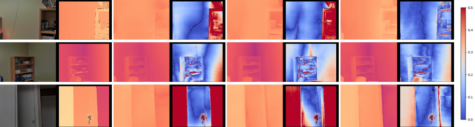
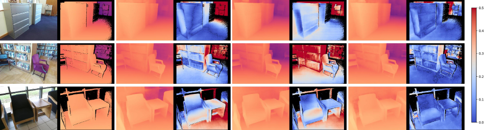
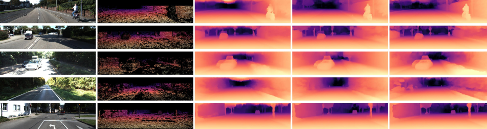
Image                GT                         AdaBins[5]                            NeWCRF[64]                              Ours

Figure 11: Qualitative results on Diode. Each row corresponds to one zero-shot test sample for the model trained on NYU and tested on Diode. The first two columns correspond to the input image and depth GT, respectively. Each subsequent couple corresponds to the pair output depth and error map. Error maps are clipped at 0.5m and the corresponding colormap is coolwarm.

Image                GT                         AdaBins[5]                            NeWCRF[64]                              Ours

Figure 12: Qualitative results on SUN-RGBD. Each row corresponds to one zero-shot test sample for the model trained on NYU and tested on SUN-RGBD. The first two columns correspond to the input image and depth GT, respectively. Each subsequent couple corresponds to the pair output depth and error map. Error maps are clipped at 0.5m and the corresponding colormap is coolwarm.

Image                                GT                            AdaBins[5]                     NeWCRF[64]                           Ours

Figure 13: Qualitative results on KITTI. Each row corresponds to a test sample from KITTI. The first two columns correspond to the input image and depth GT, respectively. The following columns correspond to the respective models trained on KITTI.

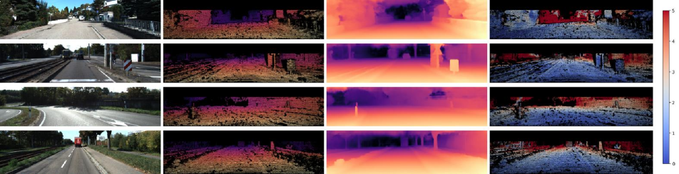
Image                                        GT                                        Ours                                        Error

Figure 14: Failure cases on KITTI. Each row corresponds to one test sample from KITTI Eigen-split validation set. The examples selected correspond to the four worst samples in terms of absolute error. Error maps are clipped at 5m and the corresponding colormap is coolwarm.

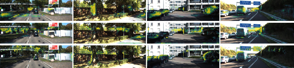
Figure 15: Attention maps on KITTI for three different IDRs. Each row presents the attention map of a specific IDR for four test images. Each IDR focuses on a specific high-level concept. The first two rows pertain to IDR at the lowest resolution while the last corresponds to the highest resolution. Best viewed on a screen and zoomed in.

References

- [1] Ashutosh Agarwal and Chetan Arora. Attention attention everywhere: Monocular depth prediction with skip attention. 2023 IEEE/CVF Winter Conference on Applications of Computer Vision (WACV), pages 5850–5859, 2022.
- [2] Lei Jimmy Ba, Jamie Ryan Kiros, and Geoffrey E. Hinton. Layer normalization. arXiv e-prints, abs/1607.06450, 2016.
- [3] Gwangbin Bae, Ignas Budvytis, and Roberto Cipolla. Estimating and exploiting the aleatoric uncertainty in surface normal estimation. Proceedings of the IEEE International Conference on Computer Vision, pages 13117–13126, 9 2021.
- [4] Gwangbin Bae, Ignas Budvytis, and Roberto Cipolla. Irondepth: Iterative refinement of single-view depth using surface normal and its uncertainty. In British Machine Vision Conference (BMVC), 2022.
- [5] Shariq Farooq Bhat, Ibraheem Alhashim, and Peter Wonka. Adabins: Depth estimation using adaptive bins. Proceedings of the IEEE Computer Society Conference on Computer Vision and Pattern Recognition, pages 4008–4017, 11 2020.
- [6] Shariq Farooq Bhat, Ibraheem Alhashim, and Peter Wonka. Localbins: Improving depth estimation by learning local distributions. In European Conference Computer Vision (ECCV), pages 480–496, 2022.
- [7] András Bódis-Szomorú, Hayko Riemenschneider, and Luc Van Gool. Fast, approximate piecewise-planar modeling based on sparse structure-from-motion and superpixels. Proceedings of the IEEE Computer Society Conference on Computer Vision and Pattern Recognition, pages 469–476, 9 2014.
- [8] Yuanzhouhan Cao, Zifeng Wu, and Chunhua Shen. Estimating depth from monocular images as classification using deep fully convolutional residual networks. IEEE Transactions on Circuits and Systems for Video Technology, 28:3174–3182, 5 2016.
- [9] Nicolas Carion, Francisco Massa, Gabriel Synnaeve, Nicolas Usunier, Alexander Kirillov, and Sergey Zagoruyko. End-to-end object detection with transformers. Lecture Notes in Computer Science (including subseries Lecture Notes in Artificial Intelligence and Lecture Notes in Bioinformatics), 12346 LNCS:213–229, 5 2020.
- [10] Ming Fang Chang, John Lambert, Patsorn Sangkloy, Jagjeet Singh, Slawomir Bak, Andrew Hartnett, De Wang, Peter Carr, Simon Lucey, Deva Ramanan, and James Hays. Argoverse: 3d tracking and forecasting with rich maps. Proceedings of the IEEE Computer Society Conference on Computer Vision and Pattern Recognition, 2019-June:8740–8749, 11 2019.
- [11] Anne Laure Chauve, Patrick Labatut, and Jean Philippe Pons. Robust piecewise-planar 3d reconstruction and completion from large-scale unstructured point data. Proceedings of the IEEE Computer Society Conference on Computer Vision and Pattern Recognition, pages 1261–1268, 2010.
- [12] Jia Deng, Wei Dong, Richard Socher, Li-Jia Li, Kai Li, and Li Fei-Fei. Imagenet: A large-scale hierarchical image database. In 2009 IEEE Conference on Computer Vision and Pattern Recognition, pages 248–255, 2009.
- [13] Alexey Dosovitskiy, Lucas Beyer, Alexander Kolesnikov, Dirk Weissenborn, Xiaohua Zhai, Thomas Unterthiner, Mostafa Dehghani, Matthias Minderer, Georg Heigold, Sylvain Gelly, Jakob Uszkoreit, and Neil Houlsby. An image is worth 16x16 words: Transformers for image recognition at scale. In 9th International Conference on Learning Representations, ICLR 2021, Virtual Event, Austria, May 3-7, 2021. OpenReview.net, 2021.
- [14] David Eigen, Christian Puhrsch, and Rob Fergus. Depth map prediction from a single image using a multi-scale deep network. Advances in Neural Information Processing Systems, 3:2366–2374, 6 2014.
- [15] Huan Fu, Mingming Gong, Chaohui Wang, Kayhan Batmanghelich, and Dacheng Tao. Deep ordinal regression network for monocular depth estimation. Proceedings of the IEEE Computer Society Conference on Computer Vision and Pattern Recognition, pages 2002–2011, 6 2018.
- [16] David Gallup, Jan Michael Frahm, and Marc Pollefeys. Piecewise planar and non-planar stereo for urban scene reconstruction. Proceedings of the IEEE Computer Society Conference on Computer Vision and Pattern Recognition, pages 1418–1425, 2010.
- [17] Peng Gao, Minghang Zheng, Xiaogang Wang, Jifeng Dai, and Hongsheng Li. Fast convergence of detr with spatially modulated co-attention. Proceedings of the IEEE International Conference on Computer Vision, pages 3601–3610, 8 2021.
- [18] Ravi Garg, BG Vijay Kumar, Gustavo Carneiro, and Ian Reid. Unsupervised cnn for single view depth estimation: Geometry to the rescue. In European Conference on Computer Vision, pages 740–756. Springer, 2016.
- [19] Andreas Geiger, Philip Lenz, and Raquel Urtasun. Are we ready for autonomous driving? the kitti vision benchmark suite. In Conference on Computer Vision and Pattern Recognition (CVPR), 2012.
- [20] Vitor Guizilini, Rares Ambrus, Sudeep Pillai, Allan Raventos, and Adrien Gaidon. 3d packing for self-supervised monocular depth estimation. In IEEE Conference on Computer Vision and Pattern Recognition (CVPR), 2020.
- [21] Kaiming He, Xiangyu Zhang, Shaoqing Ren, and Jian Sun. Deep residual learning for image recognition. Proceedings of the IEEE Computer Society Conference on Computer Vision and Pattern Recognition, 2016-December:770–778, 12 2015.
- [22] Dan Hendrycks and Kevin Gimpel. Bridging nonlinearities and stochastic regularizers with gaussian error linear units. arXiv e-prints, abs/1606.08415, 2016.
- [23] Geoffrey E. Hinton, Sara Sabour, and Nicholas Frosst. Matrix capsules with EM routing. In 6th International Conference on Learning Representations, ICLR, 2018.
- [24] Gao Huang, Zhuang Liu, Laurens Van Der Maaten, and Kilian Q. Weinberger. Densely connected convolutional networks. Proceedings - 30th IEEE Conference on Computer Vision and Pattern Recognition, CVPR 2017, 2017-January:2261–2269, 8 2016.
- [25] Lam Huynh, Phong Nguyen-Ha, Jiri Matas, Esa Rahtu, and Janne Heikkilä. Guiding monocular depth estimation using depth-attention volume. Lecture Notes in Computer Science (including subseries Lecture Notes in Artificial Intelligence and Lecture Notes in Bioinformatics), 12371 LNCS:581–597, 4 2020.
- [26] Iro Laina, Christian Rupprecht, Vasileios Belagiannis, Federico Tombari, and Nassir Navab. Deeper depth prediction with fully convolutional residual networks. Proceedings - 2016 4th International Conference on 3D Vision, 3DV 2016, pages 239–248, 6 2016.
- [27] Jin Han Lee, Myung-Kyu Han, Dong Wook Ko, and Il Hong Suh. From big to small: Multi-scale local planar guidance for monocular depth estimation. arXiv e-prints, abs/1907.10326, 7 2019.
- [28] Jae Han Lee, Minhyeok Heo, Kyung Rae Kim, and Chang Su Kim. Single-image depth estimation based on fourier domain analysis. Proceedings of the IEEE Computer Society Conference on Computer Vision and Pattern Recognition, pages 330–339, 12 2018.
- [29] Sihaeng Lee, Janghyeon Lee, Byungju Kim, Eojindl Yi, and Junmo Kim. Patch-wise attention network for monocular depth estimation. In Proceedings of the AAAI Conference on Artificial Intelligence, volume 35, pages 1873–1881, May 2021.
- [30] Boying Li, Yuan Huang, Zeyu Liu, Danping Zou, and Wenxian Yu. Structdepth: Leveraging the structural regularities for self-supervised indoor depth estimation. Proceedings of the IEEE International Conference on Computer Vision, pages 12643–12653, 8 2021.
- [31] Zhenyu Li, Zehui Chen, Xianming Liu, and Junjun Jiang. Depthformer: Exploiting long-range correlation and local information for accurate monocular depth estimation. arXiv e-prints, abs/2203.14211, 3 2022.
- [32] Chen Liu, Kihwan Kim, Jinwei Gu, Yasutaka Furukawa, and Jan Kautz. Planercnn: 3d plane detection and reconstruction from a single image. Proceedings of the IEEE Computer Society Conference on Computer Vision and Pattern Recognition, 2019-June:4445–4454, 12 2018.
- [33] Chen Liu, Jimei Yang, Duygu Ceylan, Ersin Yumer, and Yasutaka Furukawa. Planenet: Piece-wise planar reconstruction from a single rgb image. Proceedings of the IEEE Computer Society Conference on Computer Vision and Pattern Recognition, pages 2579–2588, 4 2018.
- [34] Fayao Liu, Chunhua Shen, Guosheng Lin, and Ian Reid. Learning depth from single monocular images using deep convolutional neural fields. IEEE Transactions on Pattern Analysis and Machine Intelligence, 38:2024–2039, 2 2015.
- [35] Ze Liu, Yutong Lin, Yue Cao, Han Hu, Yixuan Wei, Zheng Zhang, Stephen Lin, and Baining Guo. Swin transformer: Hierarchical vision transformer using shifted windows. Proceedings of the IEEE International Conference on Computer Vision, pages 9992–10002, 3 2021.
- [36] Francesco Locatello, Dirk Weissenborn, Thomas Unterthiner, Aravindh Mahendran, Georg Heigold, Jakob Uszkoreit, Alexey Dosovitskiy, and Thomas Kipf. Object-centric learning with slot attention. Advances in Neural Information Processing Systems, 2020-December, 6 2020.
- [37] Xiaoxiao Long, Cheng Lin, Lingjie Liu, Wei Li, Christian Theobalt, Ruigang Yang, and Wenping Wang. Adaptive surface normal constraint for depth estimation. Proceedings of the IEEE International Conference on Computer Vision, pages 12829–12838, 3 2021.
- [38] Ilya Loshchilov and Frank Hutter. Decoupled weight decay regularization. 7th International Conference on Learning Representations, ICLR 2019, 11 2017.
- [39] S. H.Mahdi Miangoleh, Sebastian Dille, Long Mai, Sylvain Paris, and Yagız Aksoy. Boosting monocular depth estimation models to high-resolution via content-adaptive multi-resolution merging. Proceedings of the IEEE Computer Society Conference on Computer Vision and Pattern Recognition, pages 9680–9689, 5 2021.
- [40] Pushmeet Kohli Nathan Silberman, Derek Hoiem and Rob Fergus. Indoor segmentation and support inference from rgbd images. In ECCV, 2012.
- [41] Adam Paszke, Sam Gross, Francisco Massa, Adam Lerer, James Bradbury, Gregory Chanan, Trevor Killeen, Zeming Lin, Natalia Gimelshein, Luca Antiga, Alban Desmaison, Andreas Kopf, Edward Yang, Zachary DeVito, Martin Raison, Alykhan Tejani, Sasank Chilamkurthy, Benoit Steiner, Lu Fang, Junjie Bai, and Soumith Chintala. Pytorch: An imperative style, high-performance deep learning library. In Advances in Neural Information Processing Systems 32, pages 8024–8035. Curran Associates, Inc., 2019.
- [42] Vaishakh Patil, Christos Sakaridis, Alexander Liniger, and Luc Van Gool. P3Depth: Monocular depth estimation with a piecewise planarity prior. In IEEE/CVF Conference on Computer Vision and Pattern Recognition, CVPR, pages 1600–1611. IEEE, 2022.
- [43] Xiaojuan Qi, Renjie Liao, Zhengzhe Liu, Raquel Urtasun, and Jiaya Jia. Geonet: Geometric neural network for joint depth and surface normal estimation. In 2018 IEEE Conference on Computer Vision and Pattern Recognition, CVPR 2018, Salt Lake City, UT, USA, June 18-22, 2018, pages 283–291. Computer Vision Foundation / IEEE Computer Society, 2018.
- [44] Xiaojuan Qi, Zhengzhe Liu, Renjie Liao, Philip H. S. Torr, Raquel Urtasun, and Jiaya Jia. Geonet++: Iterative geometric neural network with edge-aware refinement for joint depth and surface normal estimation. IEEE Trans. Pattern Anal. Mach. Intell., 44(2):969–984, 2022.
- [45] Siyuan Qiao, Yukun Zhu, Hartwig Adam, Alan Yuille, and Liang-Chieh Chen. Vip-deeplab: Learning visual perception with depth-aware video panoptic segmentation. In Proceedings of the IEEE/CVF Conference on Computer Vision and Pattern Recognition, pages 3997–4008, 2021.
- [46] René Ranftl, Alexey Bochkovskiy, and Vladlen Koltun. Vision transformers for dense prediction. Proceedings of the IEEE International Conference on Computer Vision, pages 12159–12168, 3 2021.
- [47] Sara Sabour, Nicholas Frosst, and Geoffrey E. Hinton. Dynamic routing between capsules. In Isabelle Guyon, Ulrike von Luxburg, Samy Bengio, Hanna M. Wallach, Rob Fergus, S. V. N. Vishwanathan, and Roman Garnett, editors, Advances in Neural Information Processing Systems 30: Annual Conference on Neural Information Processing Systems 2017, December 4-9, 2017, Long Beach, CA, USA, pages 3856–3866, 2017.
- [48] Shuran Song, Samuel P. Lichtenberg, and Jianxiong Xiao. Sun rgb-d: A rgb-d scene understanding benchmark suite. Proceedings of the IEEE Computer Society Conference on Computer Vision and Pattern Recognition, 07-12-June-2015:567–576, 10 2015.
- [49] Zhiqing Sun, Shengcao Cao, Yiming Yang, and Kris Kitani. Rethinking transformer-based set prediction for object detection. Proceedings of the IEEE International Conference on Computer Vision, pages 3591–3600, 11 2020.
- [50] Mingxing Tan and Quoc V. Le. Efficientnet: Rethinking model scaling for convolutional neural networks. 36th International Conference on Machine Learning, ICML 2019, 2019-June:10691–10700, 5 2019.
- [51] Yao-Hung Hubert Tsai, Nitish Srivastava, Hanlin Goh, and Ruslan Salakhutdinov. Capsules with inverted dot-product attention routing. arXiv e-prints, abs/2002.04764, 2020.
- [52] Igor Vasiljevic, Nicholas I. Kolkin, Shanyi Zhang, Ruotian Luo, Haochen Wang, Falcon Z. Dai, Andrea F. Daniele, Mohammadreza Mostajabi, Steven Basart, Matthew R. Walter, and Gregory Shakhnarovich. DIODE: A dense indoor and outdoor depth dataset. arXiv e-prints, abs/1908.00463, 2019.
- [53] Jingdong Wang, Ke Sun, Tianheng Cheng, Borui Jiang, Chaorui Deng, Yang Zhao, Dong Liu, Yadong Mu, Mingkui Tan, Xinggang Wang, Wenyu Liu, and Bin Xiao. Deep high-resolution representation learning for visual recognition. IEEE Transactions on Pattern Analysis and Machine Intelligence, 43:3349–3364, 8 2019.
- [54] Peng Wang, Xiaohui Shen, Bryan C. Russell, Scott Cohen, Brian L. Price, and Alan L. Yuille. SURGE: surface regularized geometry estimation from a single image. In Daniel D. Lee, Masashi Sugiyama, Ulrike von Luxburg, Isabelle Guyon, and Roman Garnett, editors, Advances in Neural Information Processing Systems, pages 172–180, 2016.
- [55] Cihang Xie, Mingxing Tan, Boqing Gong, Jiang Wang, Alan L. Yuille, and Quoc V. Le. Adversarial examples improve image recognition. Proceedings of the IEEE Computer Society Conference on Computer Vision and Pattern Recognition, pages 816–825, 11 2019.
- [56] Dan Xu, Wanli Ouyang, Xiaogang Wang, and Nicu Sebe. Pad-net: Multi-tasks guided prediction-and-distillation network for simultaneous depth estimation and scene parsing. Proceedings of the IEEE Computer Society Conference on Computer Vision and Pattern Recognition, pages 675–684, 5 2018.
- [57] Dan Xu, Wei Wang, Hao Tang, Hong Liu, Nicu Sebe, and Elisa Ricci. Structured attention guided convolutional neural fields for monocular depth estimation. Proceedings of the IEEE Computer Society Conference on Computer Vision and Pattern Recognition, pages 3917–3925, 3 2018.
- [58] Fengting Yang and Zihan Zhou. Recovering 3d planes from a single image via convolutional neural networks. Lecture Notes in Computer Science (including subseries Lecture Notes in Artificial Intelligence and Lecture Notes in Bioinformatics), 11214 LNCS:87–103, 2018.
- [59] Guanglei Yang, Hao Tang, Mingli Ding, Nicu Sebe, and Elisa Ricci. Transformer-based attention networks for continuous pixel-wise prediction. Proceedings of the IEEE International Conference on Computer Vision, pages 16249–16259, 3 2021.
- [60] Wei Yin, Yifan Liu, Chunhua Shen, and Youliang Yan. Enforcing geometric constraints of virtual normal for depth prediction. Proceedings of the IEEE International Conference on Computer Vision, pages 5683–5692, 7 2019.
- [61] Fisher Yu, Vladlen Koltun, and Thomas Funkhouser. Dilated residual networks. Proceedings - 30th IEEE Conference on Computer Vision and Pattern Recognition, CVPR 2017, 2017-January:636–644, 5 2017.
- [62] Zehao Yu, Lei Jin, and Shenghua Gao. P2net: Patch-match and plane-regularization for unsupervised indoor depth estimation. In European Conference on Computer Vision, pages 206–222, 7 2020.
- [63] Zehao Yu, Jia Zheng, Dongze Lian, Zihan Zhou, and Shenghua Gao. Single-image piece-wise planar 3d reconstruction via associative embedding. Proceedings of the IEEE Computer Society Conference on Computer Vision and Pattern Recognition, 2019-June:1029–1037, 2 2019.
- [64] Weihao Yuan, Xiaodong Gu, Zuozhuo Dai, Siyu Zhu, and Ping Tan. Neural window fully-connected crfs for monocular depth estimation. In IEEE/CVF Conference on Computer Vision and Pattern Recognition, CVPR, pages 3906–3915. IEEE, 2022.
- [65] Weidong Zhang, Wei Zhang, and Yinda Zhang. Geolayout: Geometry driven room layout estimation based on depth maps of planes. In European Conference on Computer Vision, pages 632–648. Springer Science and Business Media Deutschland GmbH, 8 2020.
- [66] Zhenyu Zhang, Zhen Cui, Chunyan Xu, Yan Yan, Nicu Sebe, and Jian Yang. Pattern-affinitive propagation across depth, surface normal and semantic segmentation. In IEEE Computer Society Conference on Computer Vision and Pattern Recognition CVPR, pages 4101–4110, 6 2019.
- [67] Brady Zhou, Philipp Krähenbühl, and Vladlen Koltun. Does computer vision matter for action? Science Robotics, 4, 5 2019.
- [68] Xizhou Zhu, Weijie Su, Lewei Lu, Bin Li, Xiaogang Wang, and Jifeng Dai. Deformable DETR: deformable transformers for end-to-end object detection. In 9th International Conference on Learning Representations ICLR, 2021.