Abstract

The nature of dark matter (DM) is one of the most relevant questions in modern astrophysics. We present a brief overview of recent results that inquire into a possible fermionic quantum nature of the DM particles, focusing mainly on the interconnection between the microphysics of the neutral fermions and the macrophysical structure of galactic halos, including their formation both in the linear and non-linear cosmological regimes. We discuss the general relativistic Ruffini-Argüelles-Rueda (RAR) model of fermionic DM in galaxies, its applications to the Milky Way, the possibility that the Galactic center harbors a DM core instead of a supermassive black hole (SMBH), the S-cluster stellar orbits with an in-depth analysis of the S2’s orbit including precession, the application of the RAR model to other galaxy types (dwarf, elliptic, big elliptic and galaxy clusters), and universal galaxy relations. All the above focusing on the model parameters constraints, most relevant to the fermion mass. We also connect the RAR model fermions with particle physics DM candidates, self-interactions, and galactic observables constraints. The formation and stability of core-halo galactic structures predicted by the RAR model and their relation to warm DM cosmologies are also treated. Finally, we briefly discuss how gravitational lensing, dynamical friction, and the formation of SMBHs can also probe the DM nature.

1 1 0 https://doi.org/ Fermionic dark matter: physics, astrophysics, and cosmology Fermionic dark matter C. R. Argüelles ^{1,2,3,†,∗}, E. A. Becerra-Vergara ^{2,3,4,†,∗}, J. A. Rueda ^{2,3,5,6,7†,∗} and R. Ruffini^2,3,8†,∗ C. R. Arguüelles, E. A. Becerra-Vergara, J. A. Rueda and R. Ruffini Arguüelles, C. R.; Becerra-Vergara, E. A.; Rueda, J. A.; Ruffini, R. Correspondence: carguelles@fcaglp.unlp.edu.ar (C.R.A.); jorge.rueda@icra.it (J.A.R.); eduar.becerra@icranet.org (E.A.B-V.); ruffini@icra.it (R.R.) These authors contributed equally to this work.

1 Introduction

The main evidence for the existence of dark matter (DM) is implied by its gravitational effects in a plethora of astrophysical and cosmological environments, including the cosmic microwave background (CMB), baryon acoustic oscillations (BAO), galactic structures (its formation, evolution, and morphology), gravitational lensing, stellar streams, and many others. However, understanding its nature and precise overall mass distribution in galactic structures within a particle DM paradigm are still open questions.

Several attempts have been made to explain this phenomenon through ordinary matter, including active neutrinos Bond et al. (1980); Hut and White (1984) or macroscopic objects such as MACHOS Alcock et al. (2000). However, a microscopic origin of the DM particles regarding a new particle species not included in the Standard Model remains the most likely hypothesis Bertone et al. (2005); Bertone and Tait (2018).

More recent cosmological observations obtained in the last three decades have favored the adoption of the $\Lambda$CDM paradigm Bahcall et al. (1999); Ivanov et al. (2020): in the standard scheme, the DM is assumed to be produced in thermal equilibrium via weak interactions with the primordial plasma and modeled as collisionless after its decoupling from the other particle species. In this scenario, the DM decoupling is assumed to occur at a temperature smaller than the DM rest mass, so the distribution corresponds to non-relativistic particles. The traditional DM candidate within this paradigm is the so-called weakly interacting massive particle (WIMP), typically a heavy neutral lepton with masses around $100$ GeV/c² Bertone and Tait (2018). Nonetheless, many other DM candidates exist either of bosonic or fermionic nature, such as axion-like particles or sterile neutrinos, respectively, with somewhat different early Universe decoupling regimes relative to WIMPs, though still in agreement with current cosmological observables (see, e.g., Marsh (2016); Adhikari et al. (2017) for extensive reviews in the case of axions and sterile neutrinos respectively).

Besides their different early Universe physics, these different DM particles imply different outcomes in the non-linear regime of structure formation, which may allow favoring one candidate over the other. These non-linear processes typically correspond to the gravitational collapse of primordial self-gravitating DM structures such as DM halos, in which the quantum nature of the DM particles (either bosonic or fermionic) can cause distinguishable patterns which data can test. Their effects on the precise shape and stability of the DM density profiles, including the distinctive quantum effects (e.g., quantum pressure) through the central regions of the halos, may open new important avenues of research in the field. Indeed, in Schive et al. (2014), it has been shown that these interesting quantum imprints in the DM halos exist for bosonic DM, and in Argüelles et al. (2021) for fermionic DM.

A key motivation to include the quantum nature of the particles in the study of DM halos is the limited inner spatial resolution obtained within cosmological N-body simulations for such formed structures. It encompasses huge uncertainties in (1) the central DM mass distributions; (2) the relation/effects with the supermassive black hole (SMBH) at the center of large galaxies; and (3) the relationship with the baryonic matter on inner-intermediate halo scales, among others. Indeed, using classical (rather than quantum) massive pseudo-particles as the matter building blocks in N-body simulations within the $\Lambda$CDM cosmology does not allow testing quantum pressure effects in DM halos.

Increasing attention has been given in the last decade to the study of DM halos in terms of quantum particles, given they may alleviate/resolve many of the drawbacks still present in the traditional CDM paradigm on small-scales (i.e., typically below $\sim 10$ kpc scales). The bulk of these models is comprised of the following three categories:

(i) Ultralight bosons with masses $m_{b}c^{2}\sim 1$–$10\times 10^{-22}$ eV, known as ultralight DM, Fuzzy DM, or even scalar field DM Ruffini and Bonazzola (1969); Baldeschi et al. (1983); Sin (1994); Hu et al. (2000); Matos and Arturo Ureña-López (2001); Robles and Matos (2012); Suárez and Chavanis (2017); Hui et al. (2017); Bar et al. (2018); Mocz et al. (2020); Chavanis (2021).

(ii) The case of fully-degenerate fermions (i.e., in the zero temperature approximation under the Thomas-Fermi approach) with masses $m_{\rm df}c^{2}\sim$ few $\times 10^{2}$ eV Destri et al. (2013); Domcke and Urbano (2015); Randall et al. (2017); Chavanis (2022). Or the case of self-gravitating fermions but distributed in the opposite limit, that is, in the dilute regime (i.e., in Boltzmannian-like fashion) which, however, do not imply an explicit particle mass dependence when contrasted with halo observables (see, e.g., de Vega et al. (2014)).

(iii) The more general case of self-gravitating fermions in a semi-degenerate regime (i.e., at finite temperature), which can include both regimes in the same system: that is, to be highly degenerate in the center and more diluted in the outer region (see Gao et al. (1990); Chavanis (1998); Bilic et al. (2002); Chavanis et al. (2015); Chavanis (2022) for a list of generic works). Recently, the phenomenology of this theory to the study of DM in real galaxies (using specific boundary conditions from observations), was developed in full general relativity either including for escape of particles Argüelles et al. (2018, 2019); Becerra-Vergara et al. (2020, 2021); Argüelles et al. (2022, 2023) or not (Ruffini et al. (2015)), and leading to particle masses in the range $m_{f}c^{2}\sim$ few $10$–$100$ keV. The latter model is usually referred to in the literature as the Ruffini-Argüelles-Rueda (RAR) model (it has been sometimes called the relativistic fermionic-King model).

A relevant aspect of the above models is the DM particle mass dependence on the density profiles, which differs from phenomenological profiles used to fit results from classical N-body numerical simulations. Moreover, these type of self-gravitating systems of DM opens the possibility of having access to the very nature, mass, and explicit dependence on their phase-space distributions at the onset of DM halo formation in real galaxies (see, e.g.,  Hui et al. (2017) and refs. therein, for bosons and, e.g. Argüelles et al. (2019, 2021); Chavanis (2022) and refs. therein, for fermions).

In this review, we will focus on fermionic candidates as described in (iii), describe the huge progress in the last decade in their theory and phenomenology, and comment on future perspectives. This work is organized as follows. In Section 2, we recall the main features of the RAR model, the theoretical framework including the fermion equation of state (EOS), the general relativistic equations of equilibrium, and the properties of the solutions such as the DM density profile and galactic rotation curves. Section 3 is devoted to applying the RAR model to the description of the MW, so the constraint that the Galactic data of the rotation curves impose on the fermion mass. Special emphasis is also given to the high-quality data of the motion of the S-cluster stars in the proximity of Sgr A*. We outline in Section 4 the application of the RAR model to other galaxy types, specifically to dwarf spheroidal, spiral, and elliptical galaxies, as well as galaxy clusters. The extension of the model to various galaxies allows us to verify its agreement with universal observational correlations. Section 5 discusses this topic. Section 6 discusses the possibility of the sterile neutrinos being the massive fermions of the RAR model, including the constraints on possible fermion self-interactions. Section 7 discusses the formation and stability of the fermionic DM from a cosmological evolution viewpoint, e.g., the non-linear structure and the relation with warm DM cosmologies. Section 8 outlines some additional astrophysical systems and observations that can help to constrain DM models, e.g., the gravitational lensing, the DM dynamical friction on the motion of binaries, and the link between DM halos and SMBHs at the centers of active galaxies. Finally, Section 9 concludes.

2 The RAR model: theoretical framework

The RAR model was proposed to evaluate the possible manifestation of the dense quantum core - classical halo distribution in the astrophysics of real galaxies, i.e., as a viable possibility to establish a link between the dark central cores to DM halos within a unified approach in terms of DM fermions Ruffini et al. (2015). The RAR model equilibrium equations consist of the Einstein equations in spherical symmetry for a perfect fluid energy-momentum tensor. The Fermi-Dirac statistics gives the pressure and density, while the closure relations are determined by the Klein and Tolman thermodynamic equilibrium conditions Ruffini et al. (2015). The solution to this system of equations leads to continuous and novel profiles for galactic dark matter halos, whose global morphology depends on the fermionic particle mass. Such morphology has a universal behavior of the type dense core - dilute halo that extends from the center to the galactic halo, which allows providing solutions to various tensions faced by standard cosmological paradigms on galactic scales. The outermost part of such distributions makes it possible to explain the galactic rotation curves (in a similar way as traditional dark matter profiles do), while their central morphology is characterized by high concentrations of semi-degenerate fermions (due to the Pauli exclusion principle) with important astrophysical consequences for galactic nuclei (see Siutsou et al. (2015); Argüelles and et al. (2016); Mavromatos et al. (2017) for its applications). Similar core-halo profiles with applications to fermionic DM were obtained in Bilic et al. (2002) and more recently in Chavanis et al. (2015) from a statistical approach within Newtonian gravity.

The above corresponds to the original version of the RAR model, with a unique family of density profile solutions that behaves as $\rho(r)\propto r^{-2}$ at large radial distances from the center. This treatment was extended in Argüelles et al. (2018) by introducing a cutoff in momentum space in the distribution function (DF) (i.e., accounting for particle-escape effects) that allows defining the galaxy border. The extended RAR model conceives the DM in galaxies as a general relativistic self-gravitating system of massive fermions (spin $1/2$) in hydrostatic and thermodynamic equilibrium. Following Argüelles et al. (2018), we solve the Tolman–Oppenheimer–Volkoff (TOV) equations using an equation of state (EOS) that takes into account (i) relativistic effects of the fermionic constituents, (ii) finite temperature effects, and (iii) particle escape effects at large momentum ($p$) through a cutoff in the Fermi-Dirac distribution $f_{c}$,

$$f_{c}(\epsilon\leq\epsilon_{c})=\frac{1-e^{(\epsilon-\epsilon_{c})/k_{B}T}}{e^{(\epsilon-\mu)/k_{B}T}+1},\qquad f_{c}(\epsilon>\epsilon_{c})=0\,,$$ (1)

where $\epsilon=\sqrt{c^{2}p^{2}+m^{2}c^{4}}-mc^{2}$ is the particle kinetic energy, $\epsilon_{c}$ is the cutoff particle energy, $\mu$ is the chemical potential from which the particle rest-energy is subtracted, $T$ is the temperature, $k_{B}$ is the Boltzmann constant, $c$ is the speed of light, and $m$ is the fermion mass.

This extended version of the RAR model differs from the original one presented in Ruffini et al. (2015) only in condition (iii). The inclusion of the cutoff parameter allows a more realistic description of galaxies since it allows us (1) to model their finite size and (2) to apply relaxation mechanisms that realize in nature the Fermi-Dirac distribution in Eq. (1), where the entropy can reach a maximum, unlike the original RAR model with no particle escape condition, i.e., $\epsilon_{c}\rightarrow\infty$ (see Chavanis et al. (2015) for a discussion). In fact, it is important to highlight that quantum phase-space distribution (Eq. 1) can be obtained from a maximum entropy production principle Chavanis (1998). It has been shown that there is a stationary solution of a generalized Fokker-Planck equation for fermions that includes the physics of violent relaxation and evaporation, appropriate within the non-linear stages of galactic DM halo structure formation Chavanis (1998). The full set of dimensionless parameters of the model are

$$\beta=k_{B}T/(mc^{2}),\qquad\theta=\mu/(k_{B}T),\qquad W=\epsilon_{c}/(k_{B}T),$$ (2)

where $\beta$, $\theta$, and $W$ are the temperature, degeneracy, and cutoff parameters, respectively. We do not consider anti-fermions because the temperature fulfills $T\ll mc^{2}/k_{B}$.

The stress-energy tensor is that of fermionic gas modeled as a perfect fluid,

$$T^{\alpha\nu}=\mathrm{diag}\left[c^{2}\rho(r),P(r),P(r),P(r)\right],$$ (3)

whose density and pressure are associated with the distribution function $f_{c}$,

$$\rho=m\frac{2}{h^{3}}\int_{0}^{\epsilon_{c}}f_{c}(p)\left(1+\frac{\epsilon(p)}{mc^{2}}\right)d^{3}p\ ,$$ (4)

$$P=\frac{1}{3}\frac{4}{h^{3}}\int_{0}^{\epsilon_{c}}f_{c}(p)\,\epsilon\,\frac{1+\epsilon(p)/2mc^{2}}{1+\epsilon(p)/mc^{2}}d^{3}p,$$ (5)

where the integration is carried out over the momentum space bounded by $\epsilon\leq\epsilon_{c}$.

The system is considered to be spherically symmetric, so we adopt the metric

$$ds^{2}=e^{\nu(r)}{\rm d}t^{2}-e^{\lambda(r)}{\rm d}r^{2}-r^{2}{\rm d}\theta^{2}+r^{2}\sin^{2}{\theta}{\rm d}\phi^{2},$$ (6)

where ($r$,$\theta$,$\phi$) are the spherical coordinates, the metric functions $e^{\nu(r)}$ and $e^{-\lambda(r)}=1-2M(r)/r$ are functions of $r$, and $M(r)$ is the mass function. The Tolman (1930) and Klein (1949) thermodynamic equilibrium conditions, as well as the cutoff Merafina and Ruffini (1989) condition obtained from energy conservation along a geodesic, can be written as

$$e^{\nu/2}T ={\rm constant},$$ (7a)

$$e^{\nu/2}(\mu+mc^{2}) ={\rm constant},$$ (7b)

$$e^{\nu/2}(\epsilon+mc^{2}) ={\rm constant}.$$ (7c)

We set the constants on the right-hand side of Eqs. (7a)–(7c) by evaluating the equations at the boundary radius, say $r_{b}$. For instance, the escape energy condition (7c) becomes

$$\left(1+W\beta\right)=e^{(\nu_{b}-\nu)/2},$$ (8)

being $\nu_{b}\equiv\nu(r_{b})$, $W(r_{b})=\epsilon_{c}(r_{b})=0$ Merafina and Ruffini (1989). This condition approaches the Newtonian escape velocity condition, $v^{2}_{e}=-2\Phi$, in the weak-field, non-relativistic limit, $c\to\infty$ and $e^{\nu/2}\approx 1+\Phi/c^{2}$, where $\Phi$ is the Newtonian gravitational potential, and setting $\Phi(r_{b})=0$.

Therefore, the Einstein equations together with the equilibrium conditions (7a)–(8) form the following system of coupled non-linear ordinary integrodifferential equations

$$\frac{d\hat{M}}{d\hat{r}} =4\pi\hat{r}^{2}\hat{\rho},$$ (9a)

$$\frac{d\theta}{d\hat{r}} =-\frac{1-\beta_{0}(\theta-\theta_{0})}{\beta_{0}}\frac{\hat{M}+4\pi\hat{P}\hat{r}^{3}}{\hat{r}^{2}(1-2\hat{M}/\hat{r})},$$ (9b)

$$\frac{d\nu}{d\hat{r}} =\frac{2(\hat{M}+4\pi\hat{P}\hat{r}^{3})}{\hat{r}^{2}(1-2\hat{M}/\hat{r})},$$ (9c)

$$\beta(\hat{r}) =\beta_{0}e^{\frac{\nu_{0}-\nu(\hat{r})}{2}},$$ (9d)

$$W(\hat{r}) =W_{0}+\theta(\hat{r})-\theta_{0}\,,$$ (9e)

where the subscript ‘$0$’ stands for variable evaluated at $r=0$. We have introduced dimensionless quantities: $\hat{r}=r/\chi$, $\hat{M}=GM/(c^{2}\chi)$, $\hat{\rho}=G\chi^{2}\rho/c^{2}$, $\hat{P}=G\chi^{2}P/c^{4}$, with $\chi=2\pi^{3/2}(m_{\rm Pl}/m)\hbar/(mc)$, being $m_{\rm Pl}=\sqrt{\hbar c/G}$ the Planck mass. Equations (9a) and (9b) are the relevant Einstein equations, Eq. (9c) is a convenient combination of the Klein and Tolman relations for the gradient of $\theta=\mu/(k_{B}T)$, and Eq. (9e) is a direct combination of the Klein and cutoff energy conditions. Note that in the limit $W\rightarrow\infty$ (no particle escape: $\epsilon_{c}\rightarrow\infty$), the above equation system reduces to the equations obtained in the original RAR model Ruffini et al. (2015).

Argüelles et al. (2018) have shown that including the cutoff parameter, besides its theoretical relevance, allows handling more stringent outer halo constraints and leads to central cores with higher compactness compared to the ones produced by the unbounded solutions of the original RAR model Ruffini et al. (2015).

3 Constraints on fermionic DM from the Milky Way

Therefore, in the RAR model, the distribution of DM in the galaxy is calculated self-consistently by solving the Einstein equations, subjected to thermodynamic equilibrium conditions. The system of equations must be subjected to boundary conditions to satisfy galactic observables. In this section, we summarize the most relevant example, the case of the Milky Way (MW).

3.1 The Milky Way rotation curves

Thanks to the vast amount of rotation curve data (from the inner bulge to outer halo) Sofue (2013), our Galaxy is the ideal scenario to test the RAR model. The observational data used in Sofue (2013) varies from a few pc to a few $100$ kpc, covering various orders of magnitude of the radial extent with different baryonic and dark mass structures, and can go down to the $\sim 10^{-4}$ pc scale when including the S-cluster stars Gillessen et al. (2017). To fit the observed rotation curve, and according to Sofue (2013), the following matter components of the MW must be assumed:

1. A central region ($r\sim 10^{-4}$–$2$ pc) of young stars and molecular gas whose dynamic is dictated by a dark and compact object centered at Sgr A*.

2. An intermediate spheroidal bulge structure ($r\sim 2$–$10^{3}$ pc) composed mostly of older stars, with inner and main mass distributions explained by the exponential spheroid model.

3. An extended flat disk ($r\sim 10^{3}$–$10^{4}$ pc) including star-forming regions, dust, and gas, whose surface mass density is described by an exponential law.

4. A spherical halo ($r\sim 10^{4}$–$10^{5}$ pc) dominated by DM, followed by a decreasing density tail with a slope steeper than $r^{-2}$.

Considering the previous mass distributions for the Galaxy, the extended RAR model was successfully applied to explain the MW rotation curve as shown in Figs. 1 and 2, implying a more general dense core – diluted halo behavior for the DM distribution:

• A DM core with radius $r_{c}$ (defined at the first maximum of the twice-peaked rotation curve), whose value is shown to be inversely proportional to the particle mass $m$, in which the density is nearly uniform. This central core is supported against gravity by the fermion degeneracy pressure, and general relativistic effects are appreciable.

• Then, there is an intermediate region characterized by a sharply decreasing density where quantum corrections are still important, followed by an extended and diluted plateau. This region extends until the halo scale-length $r_{h}$ is achieved (defined at the second maximum of the rotation curve).

• Finally, the DM density reaches a Boltzmann regime supported by thermal pressure with negligible general relativistic effects. It shows a behavior $\rho\propto r^{-n}$ with $n>2$ that is due to the phase-space distribution cutoff. This leads to a DM halo bounded in radius (i.e., $\rho\approx 0$ occurs when the particle escape energy approaches zero).

The different regimes in the density profiles are also revealed in the DM rotation curve showing (see right panel of Fig. 1):

• A linearly increasing circular velocity $v\propto r$ reaching a first maximum at the quantum core radius $r_{c}$.

• a Keplerian power law, $v\propto r^{-1/2}$, with decreasing behavior representing the transition from quantum degeneracy to the dilute regime. After a minimum, highlighting the plateau, the circular velocity follows a linear trend until reaching the second maximum, which is adopted as the one-halo scale length in the fermionic DM model.

• A decreasing behavior consistent with the power-law density tail $\rho\propto r^{-n}$ due to the cutoff constraint.

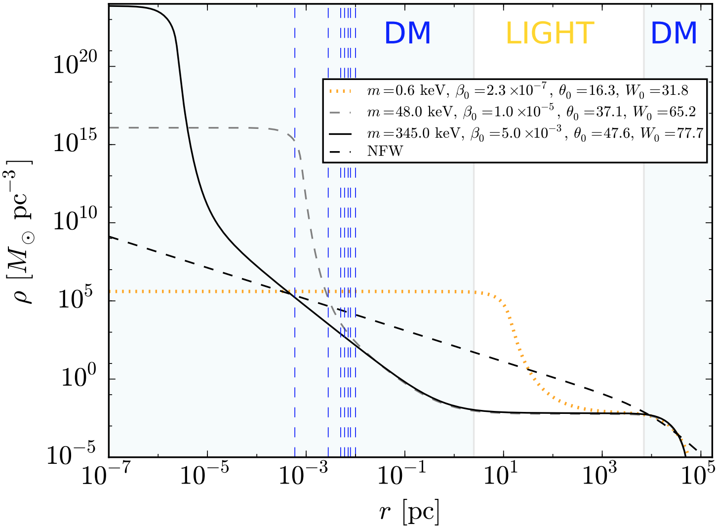
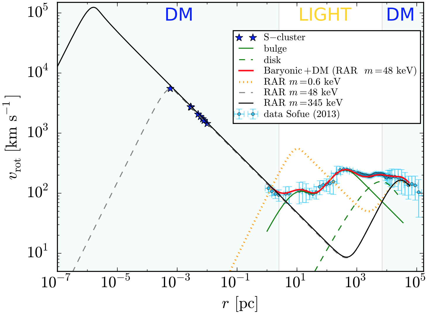
Figure 1: DM density profiles (left) and rotation curves (right), from $10^{-7}$ pc to $10^{5}$ pc, for three representative fermion masses $mc^{2}=0.6$, $48$, and $345$ keV. The vertical dashed blue lines in the left plot indicate the position of the S-cluster stars Gillessen et al. (2009), and the dashed black curve represents the NFW density profile obtained in Sofue (2013). Reprinted from Argüelles et al. (2018), Copyright (2018), with permission from Elsevier.

The Galaxy data analysis allowed us to rule out the fermion mass range $mc^{2}<10$ keV because the corresponding rotation curve starts to exceed the total velocity observed in the baryon-dominated region. On the other hand, by focusing only on the quantum core, it was possible to derive constraints that further limit the allowed fermion mass to $mc^{2}\approx 48$–$345$ keV. The dynamics of the S-cluster give the mass a lower bound. The S-stars analysis made through a simplified circular velocity analysis in general relativity showed that the fermion mass should be $mc^{2}\geq 48$ keV. Namely, the quantum core radius of the solutions for $mc^{2}<48$ keV are always greater than the radius of the S2 star pericenter, i.e., $r_{c}>r_{p_{(S2)}}=6\times 10^{-4}$ pc, which rules out fermions lighter than $48$ keV. The mass upper bound of $mc^{2}=345$ keV corresponds to the last stable configuration before reaching the critical mass for gravitational collapse, $M^{\rm cr}_{c}\propto m^{3}_{\rm Pl}/m^{2}$ Argüelles et al. (2018); Argüelles and Ruffini (2014); Argüelles et al. (2014).

As was explicitly shown in Argüelles et al. (2019, 2019, 2018), this new type of dense core – diluted halo density profile suggests that the DM might explain the mass of the dark compact object in Sgr A* as well as the halo mass. It applies not only to the MW but also to other galactic structures, from dwarfs and ellipticals to galaxy clusters Argüelles et al. (2019). Specifically, an MW analysis Argüelles et al. (2018) has shown that this DM profile can indeed explain the dynamics of the closest S-cluster stars (including S2) around Sgr A*and to the halo rotation curve without changing the baryonic bulge-disk components (see Figs. 1 and 2). Therefore, for a fermion mass between $48$–$345$ keV, the RAR solutions explain the Galactic DM halo and, at the same time, provide a natural alternative to the central BH scenario.

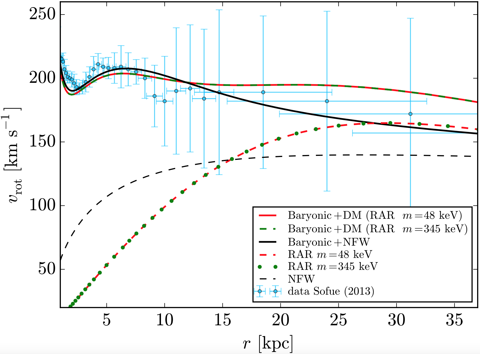
Figure 2: Zoom of the most relevant curves in the $1$–$35$ kpc region and in the linear scale of the plot in the right panel of Fig. 1. The graphic allows us to appreciate better the difference between the diverse DM models in the radial window where the Rotation Curve is most relevant. Reprinted from Argüelles et al. (2018), Copyright (2018), with permission from Elsevier.

3.2 The orbits of S2 and G2

The extensive and continuous monitoring of the closest stars to the Galactic center has produced, over decades, a large amount of high-quality data on their positions and velocities. The explanation of these data, especially the S2 star motion, reveals a compact source, Sagittarius A* (Sgr A*), whose mass must be about $4\times 10^{6}~{}M_{\odot}$. This result has been the protagonist of the Nobel Prize in Physics 2020 to Reinhard Genzel and Andrea Ghez for the discovery of a supermassive compact object at the centre of our galaxy. Traditionally, the nature of Sgr A* has been attributed to a supermassive black hole (SMBH), even though direct proof of its existence is absent. Further, recent data on the motion of the G2 cloud show that its post-peripassage velocity is lower than expected from a Keplerian orbit around the hypothesized SMBH. An attempt to overcome this difficulty has used a friction force, produced (arguably) by an accretion flow whose presence is also observationally unconfirmed.

We have advanced in Argüelles et al. (2018) and in Becerra-Vergara et al. (2020, 2021); Argüelles et al. (2021) an alternative scenario that identifies the nature of the supermassive compact object in the MW center, with a highly concentrated core of DM made of fermions (referred from now on as darkinos). The existence of a high-density core of DM at the center of galaxies had been demonstrated in Ruffini et al. (2015), where it was shown that core-halo profiles are obtained from the RAR fermionic DM model. The DM galactic structure is calculated in the RAR model treating the darkinos as a self-gravitating system at finite temperatures, in thermodynamic equilibrium, and in general relativity. It has already been shown that this model, for darkinos of $48$–$345$ keV, successfully explains the observed halo rotation curves of the MW (Argüelles et al., 2018) and other galaxy types (Argüelles et al., 2019).

Therefore, since 2020 we move forward by performing first in Becerra-Vergara et al. (2020) and then in Becerra-Vergara et al. (2021); Argüelles et al. (2021, 2022), observational tests of the theoretically predicted dense quantum core at the Galactic center within the DM-RAR model. Namely, to test whether the quantum core of darkinos could work as an alternative to the SMBH scenario for SgrA*. For this task, the explanation of the multiyear accurate astrometric data of the S2 star around Sgr A*, including the relativistic redshift that has recently been verified, is particularly important. Another relevant object is G2, whose most recent observational data, as we have recalled, challenge the scenario of an SMBH.

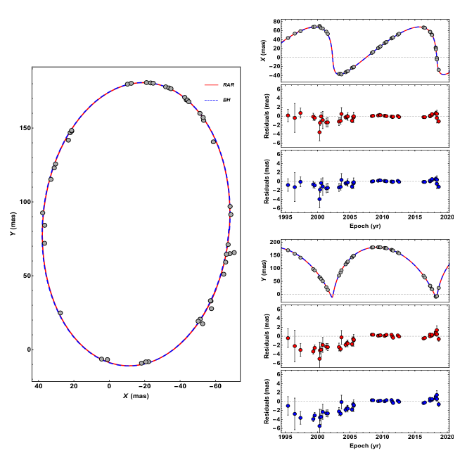
Figure 3: Theoretical (central BH and RAR models) and observed orbit of S2 around Sgr A*. The left panel shows the orbit, i.e., the right ascension ($X$) vs. declination ($Y$), while the right panel shows $X$ and $Y$ vs. observation time, with the residuals of the best-fit for the BH (blue) and the RAR (red) models. The theoretical models are calculated by solving the equations of motion of a test particle in the gravitational field of 1) a Schwarzschild BH of $4.075\times 10^{6}~{}M_{\odot}$, and 2) the DM-RAR model for $56$ keV-fermions (leading to a quantum core mass $3.5\times 10^{6}~{}M_{\odot}$). Reproduced from Becerra-Vergara et al. (2020) with permission from Astronomy & Astrophysics, Copyright ESO.

We show in Becerra-Vergara et al. (2020) that the solely gravitational potential of such a DM profile for a fermion mass of $56$ keV explains (see Figs. 3 and 4):

1. all the available time-dependent data of the position (orbit) and line-of-sight radial velocity (redshift function $z$) of S2,

2. the combination of the special and general relativistic redshift measured for S2,

3. the currently available data on the orbit and $z$ of G2,

4. its post-pericenter passage deceleration without introducing a drag force.

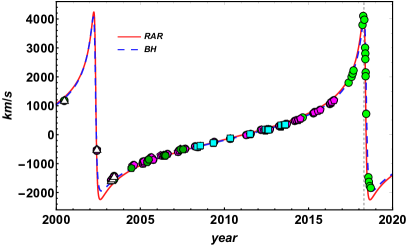
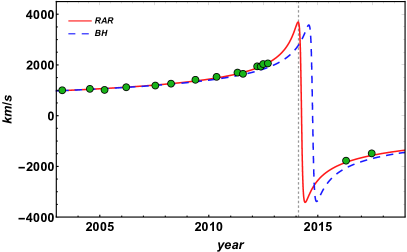
Figure 4: Theoretical and observed line-of-sight radial velocity for S2 (left) and G2 (right), calculated for the same models as in Fig. 3. Both models can fit the data with similar precision S2, and for G2, the RAR model fits the data with noticeably better precision than the BH. Reproduced from Becerra-Vergara et al. (2020) with permission from Astronomy & Astrophysics, Copyright ESO.

For both objects, it was found that the RAR model fits the data better than the BH scenario. The reduced chi-squares of the time-dependent orbit and $z$ data are $\langle\bar{\chi}^{2}\rangle_{\mathrm{S2,RAR}}\approx 3.1$ and $\langle\bar{\chi}^{2}\rangle_{\mathrm{S2,BH}}\approx 3.3$ for S2 and $\langle\bar{\chi}^{2}\rangle_{\mathrm{G2,RAR}}\approx 20$ and $\langle\bar{\chi}^{2}\rangle_{\mathrm{G2,BH}}\approx 41$ for G2. The fit of the $z$ data shows that, while for S2 the fits are comparable, i.e. $\bar{\chi}^{2}_{z,\mathrm{RAR}}\approx 1.28$ and $\bar{\chi}^{2}_{z,\mathrm{BH}}\approx 1.04$, for G2 only the RAR model fits the data: $\bar{\chi}^{2}_{z,\mathrm{RAR}}\approx 1.0$ and $\bar{\chi}^{2}_{z,\mathrm{BH}}\approx 26$. Therefore, the sole DM core, for $56$ keV fermions, explains the orbits of S2 and G2. No drag force nor other external agents are needed, i.e., their motion is purely geodesic.

The above robust analysis (and detailed in Becerra-Vergara et al. (2020)) has tested the extended RAR model Argüelles et al. (2018) with the precise astrometric data of the S2 star (and also of G2), showing an excellent agreement for a particle mass of $mc^{2}=56$ keV. Thus, it is confirmed that the elliptic orbits of these two objects moving in the surroundings of the DM-core made of $56$ keV fermions are compact enough so that the core radius $r_{c}$ is always smaller than the pericenter of the stars and have their foci coinciding with the Galactic center as obtained by observations (see, e.g., Gravity Collaboration et al. (2018)). The above results invalidate recently claimed drawbacks of the RAR model raised in Zakharov (2022) since none of the working hypotheses therein apply to the RAR model.

3.3 The orbits of all S-cluster stars

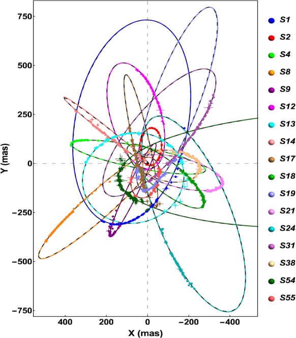
Figure 5: Best-fit orbits for the $17$ best-resolved S-star orbiting Sgr A*. It shows the projected orbit in the sky, $X$ vs. $Y$, where $X$ is right ascension and $Y$ is declination. The black dashed curves correspond to the BH model and the colored curves to the RAR model for $mc^{2}\approx 56$ keV fermions. Reproduced from Becerra-Vergara et al. (2021) with the authors’ permission.

More recently, in Becerra-Vergara et al. (2021), we have extended the above results to all the best observationally resolved S-cluster stars, namely to the up-to-date astrometry data of the $17$ S-stars orbiting Sgr A*, achieving to explain the dynamics of the S-stars with similar (and some cases better) accuracy compared to a central BH model (see Fig. 5).

Table 1 in Becerra-Vergara et al. (2021) summarizes the best-fit model parameters and reduced-$\chi^{2}$ for the position and the line-of-sight radial velocity of the $17$ S-cluster stars for the central BH and the RAR model. The average reduced-$\chi^{2}$ of the RAR model was $1.5741$ and the corresponding value of the central BH model was $1.6273$.

Therefore, a core of fermionic DM at the Galactic center explains the orbits of the S-stars with similar accuracy compared to a central BH model. The same core – halo distribution of $56$ keV fermions also explains the MW rotation curves (Argüelles et al., 2018; Becerra-Vergara et al., 2020). Data of the motion of objects near Sgr A*, if accurate enough, could put additional constraints on the fermion mass. The recently detected hot-spots apparently in a circular motion at $7$–$23~{}GM_{\rm BH}/c^{2}$ radius (Gravity Collaboration et al., 2018; Matsumoto et al., 2020), however, fail in this task because the highly-model dependence of the objects real orbit inference, including the lack of information on the object’s nature. In addition, the quality of their astrometry data is low relative to the S-stars data. We hope the data quality of these spots or similar objects can increase so that they can put relevant constraints on Sgr A* models. We keep our eyes open to the data of newly observed S-stars (S62, S4711–S4714). Their motion models based on a central BH predict they have pericenter distances $\sim 400~{}GM_{\rm BH}/c^{2}$ (Peißker et al., 2020a, b). If confirmed, these new S-stars might constrain the DM core size, so the fermion mass.

3.4 The precession of the S2 orbit

Furthermore, Argüelles et al. (2022) focused on the periapsis precession of the S2 orbit. We have there quantified, for the first time within the RAR-DM model, the effects on the S2-star periapsis (precession) shift due to an extended DM mass filling the S2 orbit, in contrast with the vacuum solution of the traditional Schwarzschild BH. The main result is as follows. While the central BH scenario predicts a unique prograde precession, in the DM scenario, it can be either retrograde or prograde, depending on the amount of DM mass enclosed within the S2 orbit, which in turn is a function of the fermion mass (see Fig. 6 and Table 6).

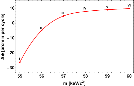
Figure 6: Relativistic periapsis precession $\Delta\phi$ per orbit as a function of the darkino mass as predicted by the RAR DM models for the S2-star. The precession is retrograde for $mc^{2}<56.4$ keV while it becomes prograde for $mc^{2}>56.4$ keV (see also Table below). Reproduced from Argüelles et al. (2022) with the authors’ permission.

Table 1: Comparison of the BH and RAR DM models that best fit all the publicly available data of the S2 orbit. The $2nd$ column shows the central object mass, $M_{\rm CO}$. For the Schwarzschild BH model, $M_{\rm CO}=M_{\rm BH}$, while for the RAR model, $M_{\rm CO}=M_{c}$, with $M_{c}$ the DM core mass. The $3rd$ column shows the radius of the central object, $r_{c}$. For the Schwarzschild BH model, $r_{c}$ is given by the event horizon radius, $R_{\rm Sch}=2GM_{\rm BH}/c^{2}$. The $4th$ column shows the DM mass enclosed within the S2 orbit, $\Delta M_{\rm DM}/M_{\rm CO}$. The best-fitting pericenter and apocenter radii of the S2 orbit are given in the $5th$ and $6th$ columns. The values of the average reduced-$\chi^{2}$ of the best fits, defined as in Becerra-Vergara et al., 2020, are given in the $7th$ column. The last two columns show the model predictions of the periapsis precession of the real orbit, $\Delta\phi$, and of the sky-projected orbit, $\Delta\phi_{\rm sky}$. Reproduced from Argüelles et al. (2022) with the authors’ permission.

Model			$M_{CO}$ $\left[10^{6}M_{\odot}\right]$		$r_{c}$ $\left[mpc\right]$		$\Delta M_{DM}/M_{CO}$		$r_{p}$ $\left[as\right]$		$r_{a}$ $\left[as\right]$		$\langle\bar{\chi}^{2}\rangle$		$\Delta\phi$ $\left[arcmin\right]$		$\Delta\phi_{sky}$ $\left[arcmin\right]$
I	RAR ($mc^{2}=55$ keV)		$3.55$		$0.446$		$1.39\times 10^{-2}$		$0.01417$		$0.23723$		$2.9719$		$-26.3845$		$-32.1116$
II	RAR ($mc^{2}=56$ keV)		$3.50$		$0.427$		$5.99\times 10^{-3}$		$0.01418$		$0.23618$		$3.0725$		$-4.9064$		$-5.9421$
III	RAR ($mc^{2}=57$ keV)		$3.50$		$0.407$		$2.21\times 10^{-3}$		$0.01417$		$0.23617$		$3.2766$		$4.8063$		$5.8236$
IV	RAR ($mc^{2}=58$ keV)		$3.50$		$0.389$		$7.13\times 10^{-4}$		$0.01424$		$0.23609$		$3.2814$		$7.7800$		$9.4243$
V	RAR ($mc^{2}=59$ keV)		$3.50$		$0.371$		$2.93\times 10^{-4}$		$0.01418$		$0.23613$		$3.3356$		$9.0456$		$10.9613$
VI	RAR ($mc^{2}=60$ keV)		$3.50$		$0.355$		$1.08\times 10^{-4}$		$0.01423$		$0.23610$		$3.3343$		$9.8052$		$11.8764$
	BH		$4.07$		$3.89\times 10^{-4}$		$0$		$0.01427$		$0.23623$		$3.3586$		$11.9501$		$14.4947$

Therefore, for larger and larger particle masses, the behavior of the RAR model tends to be that of the BH. As Fig. 6 shows, the precession tends nearly asymptotically to $12$ arcmin ($\approx 0.2$ deg), the predicted precession of a central Schwarzschild BH (see, e.g., GRAVITY Collaboration et al. (2020)). The RAR model produces the same prograde precession of a central BH for $345$ keV fermions, corresponding to the unstable DM core for gravitational collapse into a BH. For $56.4$ keV fermions, the prograde and retrograde contributions balance each other leading to a zero net precession. For lower masses, the net precession is retrograde. It has been shown in Argüelles et al. (2022) that currently, available data constrains the amount of retrograde precession, imposing a lower limit to the fermion mass of $\approx 57$ keV, hence an upper limit to the amount of mass enclosed in the orbit of $\approx 0.1\%$ of the core’s mass (see Table 1). Indeed, the latter limit agrees with the one obtained by GRAVITY Collaboration et al. (2020). For fermion masses above $57$ keV, the prograde precession of the RAR model and that of a central BH agree within the experimental uncertainties. The reason has been explained in Argüelles et al. (2022): the most accurate S2 data correspond to its pericenter passage Do et al. (2019); GRAVITY Collaboration et al. (2020), while the best place to analyze orbital precession is around the apocenter.

The above is shown in Fig. 7 that plots the relativistic precession of S2 projected orbit in a right ascension - declination plane. It can be seen that while the positions in the plane of the sky nearly coincide about the last pericenter passage in the three models, they can be differentiated close to the next apocenter. Specifically, the upper right panel evidences the difference at the apocenter between the prograde case (as for the BH and RAR model with $mc^{2}=58$ keV) and the retrograde case (i.e., RAR model with $mc^{2}=56$ keV).

The bad news is that, as evidenced by Fig. 7, all the current and publicly available data of S2 can not discriminate between the two models. The good news is that the upcoming S2 astrometry data close to the next apocentre passage could potentially establish if a classical BH or a quantum DM system governs Sgr A*.

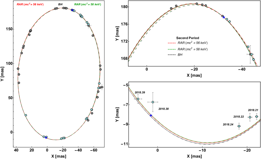
Figure 7: Relativistic precession of S2 in the projected orbit on the plane of the sky, predicted in the BH and RAR DM models. While it is prograde for the BH and RAR ($mc^{2}=58$ keV) (in dashed black and green respectively), it is retrograde for the RAR DM model ($mc^{2}=56$ keV) (in dashed red). The solid (theoretical) curves and gray (data) points correspond to the first period ($\approx 1994$–$2010$), while the dashed (theoretical) curves and cyan (data) points to the second period ($\approx 2010$–$2026$). Right panels: zoom of the region around apocenter (top panel) and pericenter (bottom panel). Reproduced from Argüelles et al. (2022) with the authors’ permission.

A further interesting consequence of this scenario is that a core made of darkinos becomes unstable against gravitational collapse into a BH for a threshold mass of $\sim 10^{8}~{}M_{\odot}$. Collapsing DM cores can provide the BH seeds for forming SMBHs in active galaxies (such as M87) without the need for prior star formation or other BH seed mechanisms involving super-Eddington accretion rates as demonstrated in Argüelles et al. (2021) from thermodynamic arguments. This topic is of major interest, and further consequences and ramifications are currently being studied, including:

• to propose a new paradigm for SMBH formation and growth in a cosmological framework, which is neither based on the baryonic matter nor early Universe physics;

• to study the problem of disk accretion around such DM-cores starting with the generalization of the Shakura & Sunyaev disk equations in the presence of a high concentration of regular matter (i.e., instead of a singularity);

• to use fully relativistic ray-tracing techniques to predict the corresponding shadow-like images around these fermion cores and compare them with the shape and sizes of the ones obtained by the EHT.

4 Fermionic DM in other galaxy types

4.1 The RAR model in dwarf, spiral, elliptical galaxies, and galaxy clusters

In the preceding section, we have shown that the RAR model can perfectly explain the MW rotation curve while providing an excellent alternative to the BH scenario in SgrA* when constrained through the dynamics of the S-cluster stars, including its relativistic effects. In this section, we summarize the main results of the RAR model when applied to different galaxy types, such as dwarfs, spirals, ellipticals, and galaxy clusters, as detailed in Argüelles et al. (2019). Thus, for the relevant case of a fermion mass of $mc^{2}\approx 50$ keV (motivated by the MW phenomenology as shown in 3), we make full coverage of the remaining free RAR model parameters ($\beta_{0}$,$\theta_{0}$,$W_{0}$) and present the complete family of density profiles which satisfy realistic halo boundary conditions as inferred from observations (see Fig. 8).

For galaxy types located far away from us, the observational inferences of their DM distributions are limited to a narrow window of galaxy radii, typically from a few up to several half-light radii. Generally, we have no access to observations for possible detection of a central dark compact object (as for SgrA* in our Galaxy) nor to constrain the system’s total (or virial) mass. Thus, we adopt here (see Argüelles et al. (2019) for further details) a similar methodology as applied to the MW (as shown in Fig. 3 and detailed in (Argüelles et al., 2018)), but only limited to halo-scales where observational data is available (i.e., we do not set any boundary mass conditions in the central core). In particular, we select as the boundary conditions a characteristic halo radius $r_{h}$ with the corresponding halo $M_{h}\equiv M(r_{h})$. The halo radius is defined as the location of the maximum in the halo rotation curve, which is defined as the one-halo scale length in the RAR model. We list below the parameters ($r_{h}$, $M_{h}$) adopted for the different DM halos as constrained from observations in typical dwarf spheroidal (dSph), spiral, elliptical galaxies, and bright galaxy clusters (BCG). We only exemplified the first three cases; see Argüelles et al. (2019) for the BCGs.

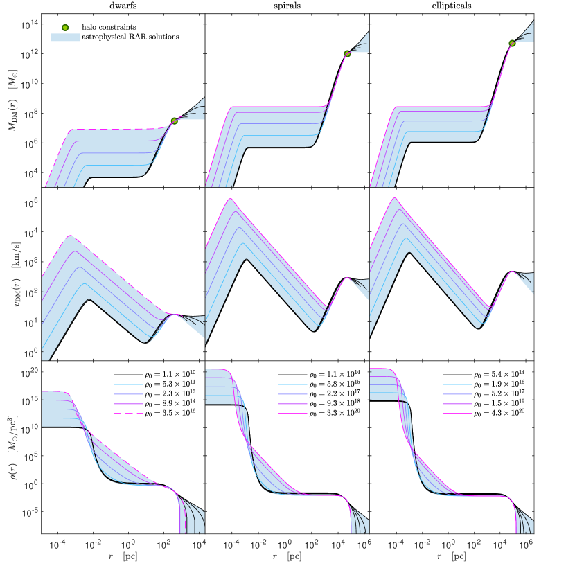
Figure 8: Astrophysical RAR solutions, for the relevant case of $mc^{2}=48$ keV, observationally fulfill given DM halo restrictions $(r_{h},M_{h})$ for typical dwarf (left), spiral (middle) and elliptical galaxies (right). Shown are density profiles (bottom), rotation curves (middle), and DM mass distributions (top). The full window for each galaxy type is illustrated by a blue shaded region and enveloped approx. by $5$ benchmark solutions inside. Each solution is labeled with the central density in units of $M_{\odot}$ pc^-3. The continuous-magenta curves, occurring only for spiral and elliptical galaxies, indicate the critical solutions which develop compact, critical cores (before collapsing to a BH) of $M_{c}^{\rm crit}=2.2\times 10^{8}M_{\odot}$. The dashed-magenta curves for dwarfs are limited (instead) by the astrophysical necessity of a maximum in the halo rotation curve. The bounding black solutions correspond to the ones having the minimum core mass (or minimum $\rho_{0}$), which in turn imply larger cutoff parameters (implying $\rho\propto r^{-2}$ when $W_{0}\to\infty$. Reprinted from Argüelles et al. (2019), Copyright (2019), with permission from Elsevier.

4.2 Typical dSph galaxies

Table 2: Typical halo radius and mass for dsPh, spirals, elliptical galaxies, and galaxy cluster, adopted in Argüelles et al. (2018) for testing the RAR model.

	typical dSph	typical spiral	typical elliptical	typical galaxy cluster
$r_{h(d)}$ (kpc)	$0.4$	$50$	$90$	$600$
$M_{h(d)}$ $(M_{\odot})$	$3\times 10^{7}$	$1\times 10^{12}$	$5\times 10^{12}$	$3\times 10^{14}$

The halo parameters in Table 2 are an average of the eight best-resolved dSphs of the MW studied in Walker et al. (2009) by solving the Jeans equations and adopting a cored-Hernquist DM profile, which is similar to the mid-outer region of the RAR profiles Argüelles et al. (2019).

4.3 Typical spiral galaxies

The halo parameters shown in Table 2 are obtained from a group of nearby disk galaxies taken from the THINGS data sample de Blok et al. (2008), where it was possible to obtain a DM model-independent evidence for a maximum in the rotation curves. This was obtained by accounting for baryonic (stars and gas) components in addition to the (full) observed rotation curve from HI tracers (see Argüelles et al. (2019), and refs. therein for details).

4.4 Typical elliptical galaxies

The halo parameters in Table 2 are obtained from (i) a sample of elliptical galaxies from Hoekstra et al. (2005), studied via weak lensing, from which in Donato et al. (2009) it was provided the corresponding halo mass models for the tangential shear of the distorted images; and (ii) the largest and closest elliptical M87 as studied in Romanowsky and Kochanek (2001), accounting for combined halo mass tracers like stars, globular clusters, and X-ray sources (see Argüelles et al. (2019), and refs. therein for further details).

4.5 Typical galaxy clusters

The halo parameters in Table 2 are obtained from a sample of $7$ BCGs from Newman et al. (2013). There, the luminous and dark components were disentangled to obtain DM distributions which were reproduced by a generalized NFW (gNFW) model Zhao (1996), developing a maximal velocity at the one-halo length scale $r_{\rm max(bcg)}$. In Newman et al. (2013), the data among all these $7$ cases (i.e., weak lensing and stellar kinematics) support such a maximum within a radial extent from $10$ kpc up to $3$ Mpc; whose corresponding averages in $r_{h}$ and $M_{h}$ are given in Table 2.

The main conclusions of having applied the RAR model for $mc^{2}\approx 50$ keV to different galaxy types are summarized as follows (see Argüelles et al. (2019) for a more detailed explanation):

1. Typical dwarf galaxies can harbor dense and compact DM cores with masses from $M_{c}\sim 10^{3}M_{\odot}$ up to $M_{c}\sim 10^{6}M_{\odot}$ (see Fig. 8), offering a natural explanation for the so-called intermediate-mass BHs (IMBH). Since the total mass of the typical dSphs here analyzed is below the critical mass of core-collapse (i.e., $M_{\rm tot(d)}\sim 10^{7}M_{\odot}<M_{c}^{\rm cr}\approx 2\times 10^{8}M_{\odot}$), the core can never become critical and thus will never collapse to a BH. Therefore, the RAR model predicts (for a particle mass of $mc^{2}\approx 50$ keV) that dSph galaxies can never develop a BH at their center, a result that may explain why these galaxies never become active.

2. Typical spiral and elliptical galaxies can harbor denser and more compact DM cores (w.r.t dSphs) with masses from $M_{c}\sim 10^{5}M_{\odot}$ up to $M_{c}^{\rm cr}\approx 2\times 10^{8}M_{\odot}$ (see Fig. 8). Thus, they offer a natural alternative to the supermassive BHs hypothesis (see Fig. 3 for the MW). Since the total mass in spirals and ellipticals is much larger than $M_{c}^{\rm cr}$, the core mass can become critical and eventually collapse towards an SMBH of $\sim 10^{8}M_{\odot}$ which may then grow even larger by accretion.

3. Typical bright cluster of galaxies (BCGs) can harbor dense and compact DM cores with masses from $M_{c}\sim 10^{6}M_{\odot}$ up to $M_{c}^{\rm cr}\approx 2\times 10^{8}M_{\odot}$ (see Fig. 8). The implications of this prediction for BCGs are still unclear, mainly given the limited spatial resolution achieved by actual observational capabilities below the central kpc. More work is needed (for example, using strong lensing observations) to evaluate if galaxy clusters show an enhancement in DM density similar to the one predicted by the RAR model.

4. By combining the range of DM core masses, inner halo densities, and total halo masses as predicted by the RAR model across all of these systems, it is possible to test whether or not this model can answer different Universal scaling relations. A point which is studied in the next section (and further detailed in Argüelles et al. (2019) and Argüelles et al. (2023)).

5 Universal galaxy scaling relations

Galaxies follow different scaling relations (or Universal scaling relations) such as the DM surface density relation (SDR) Donato et al. (2009), the radial acceleration relation McGaugh et al. (2016), the mass discrepancy acceleration relation (MDAR) McGaugh (2004) and the Ferrarese relation Ferrarese (2002); Bogdán and Goulding (2015) between the total halo mass and its supermassive central object mass. Thus, this section’s main goal is to illustrate/summarize the ability of the RAR model to agree with all these relations, covering a really broad window of radial scales across very different galaxy types. The analyses are exemplified for a fermion of rest mass-energy of $\approx 50$ keV.

For given halo parameters $(r_{h},M_{h})$ as inferred from observations in the smallest up to the largest galaxy types (see Table 2), the RAR model predicts a window of halo values on other radial-scales: (a) the plateau density (or inner-halo constant density) $\rho_{\rm pl}$; (b) the total halo mass $M_{\rm tot}$; and (c) the fermion-core mass $M_{c}$. We will then use this predictive power of the RAR model (shown Fig. 8) to test if it can answer for the above Universal scaling relations as reported in the literature. We will focus first on the Ferrarese relation between the total halo mass and its supermassive central object mass and in the SDR.

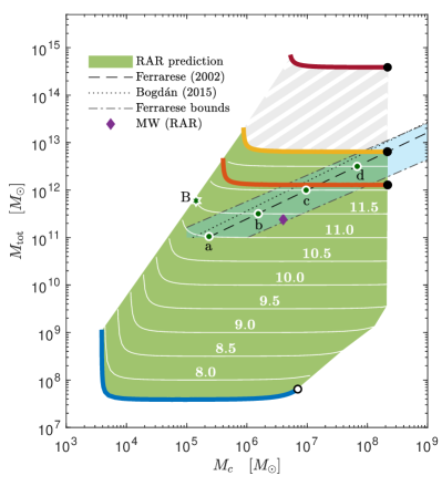
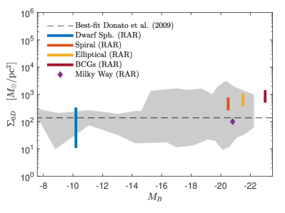
Figure 9: Left: theoretical $M_{c}$-$M_{\rm tot}$ relation within three parametric RAR model (for $mc^{2}=48$ keV). The colored lines read for each galaxy type in correspondence with the astrophysical RAR solutions in Fig. 8. The green area covers the RAR predictions for a given halo mass in the range $M_{h}\approx 10^{7}$–$10^{12}M_{\odot}$ and fulfilling $\Sigma_{0D}\propto\rho_{\rm pl}\,r_{h}=140M_{\odot}$ pc^-2, as inferred from the Donato relation (see right panel). The white lines show a set of families with given halo mass $M_{h}$ (and labeled by the $M_{\rm tot}$ value in the horizontal regime). The results show the RAR model agrees with the different $M_{\rm BH}$-$M_{\rm tot}$ relations, as considered in the literature and shown in the blue-ish stripe. The filled-black dots correspond to the critical core mass $M_{c}^{\rm crit}$, and the empty-black dot indicates the limiting maximum core mass $M_{c}^{\rm max}$ for dwarfs. Right: surface DM density (or Donato) relation as predicted by the RAR model (see vertical color lines) for each galactic structure in correspondence with the astrophysical solutions (i.e., blue-shaded regions in Fig. 8). The dashed horizontal line represents the Universal relation from the best fit of the data as found by Donato et al. (2009). The dark-gray region indicates the delimited area by the $3-\sigma$ error bars of all the data points. Reprinted from Argüelles et al. (2019), Copyright (2019), with permission from Elsevier.

5.1 The Ferrarese relation

This relation establishes that, for large enough galaxies, the more massive the halo, the larger (in mass) is the supermassive compact object lying at its center. This relation is shown in dashed in the left panel Fig. 9, as taken from Ferrarese (2002), together with other more updated versions of such relation such as the one found in Bogdán and Goulding (2015) (shown in dotted line in the same figure). Interestingly enough, the whole family of RAR solutions, with its corresponding window of predicted core and total DM masses $M_{c},M_{\rm tot}$ (see left panel of Fig. 9), from typical dwarf to ellipticals galaxies (see green area), do overlap with the Ferrarese relation. That is, the RAR model contains the observational strip (in light blue), while at the same time, it extends out such a Ferrarese strip, indicating a yet-unseen or otherwise unphysical cases (see Argüelles et al. (2019) for further details).

Even if no observational data exist yet at the down-left corner of Fig. 9 (left panel), special attention has to be given to the RAR model predictions for dwarf galaxies: recent observations towards the center of some ultra-compact dwarf galaxies of total mass few $\sim 10^{7}M_{\odot}$ (e.g., Seth et al. (2014); Ahn et al. (2017); Afanasiev et al. (2018)), indicate the existence of putative massive BH of few $\sim 10^{6}M_{\odot}$. Interestingly, the RAR model naturally allows for a slight difference (less than an order of magnitude) between $M_{c}$ and $M_{\rm tot}$. However, more work is needed on this particular dwarf galaxy to make a more definite statement.

5.2 The DM surface density relation (DSR)

The DSR relation establishes that the central surface DM density in galaxies is roughly constant, spanning more than 14 orders in absolute magnitude ($M_{B}$): $\rho_{0D}r_{0}\approx 140M_{\odot}$ pc^-2 (with $\rho_{0D}$ the inner-halo -or sometimes called central- DM halo density measured at the Burkert halo radius $r_{0}$) (Donato et al., 2009).

Since the Burkert central density corresponds to the plateau density of the RAR density profiles (see right panel of Fig. 11), i.e., $\rho_{0D}\equiv\rho_{\rm pl}$, and $r_{0}\approx 2/3\,r_{h}$ (as shown in Argüelles et al. (2019) connecting the Burkert and RAR one-halo scale-lengths), it is possible to check the DSR by calculating the product $2/3\,\rho_{\rm pl}r_{h}$ along the entire family of astrophysical RAR solutions of Section 4 (including the Milky Way). This is shown in the right panel of Fig. 9.

It can be seen that the RAR model predictions agree with the observed relation, the latter displayed in Fig. 9 (right panel) in the dark-grey region delimited (or enveloped) within the $3-\sigma$ error bars along all the data points considered in Donato et al. (2009). That figure shows that each typical galaxy type’s predicted RAR surface density (vertical solid lines) is within the expected $3-\sigma$ data region. We further notice that typical bright clusters are beyond the observed window as reported by Donato et al. (2009), who considered only up to elliptical structures.

5.3 The radial acceleration and mass discrepancy acceleration relations

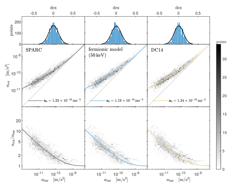
Figure 10: Radial acceleration relation (top) and mass discrepancy acceleration relation (bottom) for SPARC data and competing DM halo models. Each plot is divided into $50\times 50$ equal bins. The baryonic centripetal acceleration $\mathfrak{a}_{\rm bar}$ is inferred from luminosity observables while the total acceleration $\mathfrak{a}_{\rm tot}$ is inferred independently from velocity fields. For DM halo models, the total acceleration is composed of the predicted dark and inferred baryonic components, i.e., $\mathfrak{a}_{\rm tot}=\mathfrak{a}_{\rm DM}+\mathfrak{a}_{\rm bar}$. The corresponding solid curves are the best fits characterized by a specific $\mathfrak{a}_{0}$. The histogram plots (upper row) show a Gaussian distribution of $\log_{10}(\mathfrak{a}_{0}/\mathfrak{a}_{0})$. The grayscale legend shows the number of points per bin ($2396$ for the $120$ SPARC-galaxies used). Reproduced from Argüelles et al. (2023).

We now confront the RAR model predictions with two closely related Universal relations, though this time not based on typical galaxies with given (averaged) parameters ($r_{h},M_{h}$) inferred from observables (as done before), but from a sample of 120 rotationally supported galaxies taken from the SPARC data set Lelli et al. (2016).

The radial acceleration relation is a non-linear correlation between the radial acceleration exerted on the total matter distribution and the one caused by the baryonic matter component only (see Eq. 10 below). Thus it offers an important restriction to any model that explains the DM halo in galaxies.

The different mass components in a galaxy, like a bulge, disk, gas, etc., trace their own contribution to the centripetal or radial acceleration $\mathfrak{a}=v^{2}/r$. As originally shown in McGaugh et al. (2016), it exists a relatively tight relation between the radial acceleration owing to the total mass, say $\mathfrak{a}_{\rm tot}$, and that produced by the baryonic mass component, say $\mathfrak{a}_{\rm bar}$, which the empirical formula can well describe

$$\mathfrak{a}_{\rm tot}=\frac{\mathfrak{a}_{\rm bar}}{1-e^{-\sqrt{\mathfrak{a}_{\rm bar}/{\mathfrak{a}_{0}}}}},$$ (10)

with $\mathfrak{a}_{0}$ the only adjustable parameter. Notice that for $\mathfrak{a}_{\rm bar}\ll\mathfrak{a}_{0}$, the DM dominates, and the relation deviates from linear, while for $\mathfrak{a}_{\rm bar}\gg\mathfrak{a}_{0}$, the baryonic component dominates and the linear relation is recovered (see Fig. 10). The relation has been shown to apply applies to different galaxy types, e.g., disk, elliptical, lenticular, dwarf spheroidal, and low-surface-brightness galaxies, so it looks like a real universal law McGaugh et al. (2016); Lelli et al. (2017); Di Paolo et al. (2019).

We also include in the analysis a close relation: the mass discrepancy acceleration relation (MDAR) relation between baryonic and total mass components. It is defined by $D=M_{\rm tot}/M_{\rm bar}$ with $M_{\rm bar}$ the total baryonic mass and $M_{tot}$ the total mass content of the galaxy including the DM component. If we define the radial acceleration through its definition in terms of the gravitational potential of a spherically symmetric mass distribution, then the MDAR can be written as $D=\mathfrak{a}_{tot}/\mathfrak{a}_{\rm bar}$.

In Fig. 10, we show the results of the best fits for the radial acceleration relation and MDAR for both the RAR model (central panels) and the DC14 DM model (right panels) accounting for baryonic-feedback Di Cintio et al. (2014) (see also the full Figure 2 in Argüelles et al. (2023) for best-fits to both relations by other DM typical halo models used in the literature). Since both models achieve very close fitted values of $\mathfrak{a}_{0}\approx 1.2\times 10^{-10}$ m s^-2 as the one obtained from the SPARC data only (i.e., done in DM model-independent fashion, see left panels), then it is concluded that this Universal relation does not help to prefer one model over the other statistically (see Argüelles et al. (2023) for details). Instead, as demonstrated in Argüelles et al. (2023), the individual fitting of each rotation curve (covering the full SPARC sample studied) allows to favor of the cored profiles over the cuspy Navarro-Frenk-White profile (not shown here).

Finally, we have also compared the DM halo models by their density profiles and rotation curves for typical SPARC galaxies in the left panel of Fig. 11. Most models show similarities in the halo tails, but the RAR model is the only one showing a dense-fermion core at the galaxy’s center, which acts as an alternative to the SMBH scenario. It is also relevant to mention that while many of the models (such as Einasto or DC14) need the baryonic feedback to produce the statistically favored cored density profiles, the RAR model naturally achieves a cored behavior (i.e., the inner-halo plateau) due to the quasi-thermodynamic equilibrium of the particles at formation (see Argüelles et al. (2023) and references therein for further discussions).

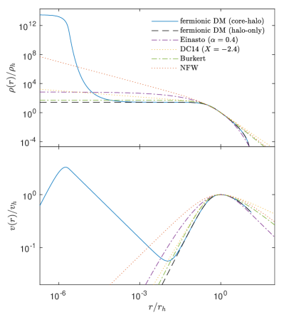
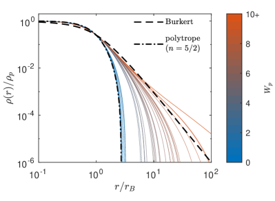
Figure 11: Left: density profile (top) and rotation curve (bottom) for selected DM models for the typical configuration parameters presented in Argüelles et al. (2023). The core-halo solution of the RAR model is illustrated by the configuration parameters $\beta_{0}=10^{-7}$, $\theta_{0}=30$ and $W_{0}=60$, in combination with a corresponding halo-only solution. Other DM models (NEW, DC14, Burkert, Einasto) are added for comparison. All profiles are normalized to the halo radius $r_{h}$, defined at the halo velocity maximum, with $\rho_{h}=r(r_{h})$ and $v_{h}=v(r_{h})$. Right: best-fit DM density RAR profiles (outer region) to the full SPARC sample considered in Argüelles et al. (2023) (in solid) for different values of the cut-off parameter $W(r_{\rm pl})\equiv W_{p}$: the outer halo of the RAR model can go from polytropic-like (polytropic index $n=5/2$ in dot-dashed) to power law-like (e.g., $\rho\propto r^{-3}$) resembling the Burkert profile (in dashed). Reproduced from Argüelles et al. (2023).

Although we do not expect significant qualitative or quantitative differences in the galaxy structure parameters for fermion masses around the above-explored value of $50$ keV, studying the implications of different fermion masses for the universal relations will be interesting. We plan to have new results on this topic soon.

6 Fermionic DM and particle physics

6.1 Are the sterile neutrinos the fermions of the RAR model?

In this section, we will discuss a possible connection to particle physics (i.e., beyond the standard model of particles), analyzing the possibility that the DM particles are self-interacting DM. Namely, DM particles interact among themselves via some unknown fundamental interaction besides gravity. It is a very active field of research within the DM community since self-interacting DM (SIDM) has been proposed as a possible solution to several challenges which is facing the standard cosmological model on galactic scales (see Mavromatos et al. (2017); Tulin and Yu (2018) for different reviews on the subject).

In 2016, our group presented an extension of the RAR model to include fermion self-interactions, referred to as the Argüelles, Mavromatos, Rueda and Ruffini (AMRR) model Argüelles et al. (2016). In the AMRR model, it has been advanced that the darkinos might be the right-handed sterile neutrinos introduced in the minimum standard model extension ($\nu$MSM) paradigm Shaposhnikov (2008). The AMRR model adopts right-handed neutrinos self-interacting via dark-sector massive (axial) vector mediators.

In 2020, Yunis et al. (2020) explored the radiative decay channel of such sterile neutrinos into X-rays due to the Higgs portal interactions of the $\nu$MSM. This work shows that such generalized RAR profiles, including fermion self-interactions, agree with the overall MW rotation curve. In addition, the window of self-interacting DM cross-sections that satisfy the known bullet cluster constraints has been identified.

To further constrain the AMRR-$\nu$MSM model, an indirect detection analysis has been performed using X-ray observations from the Galactic center by the Nustar mission Yunis et al. (2020). Figure 12 summarizes all the observational constraints.

It has also advanced a new generation mechanism based on vector-meson decay, able to produce these sterile neutrinos in the early Universe.

Summarizing, by considering a DM profile that self-consistently accounts for the particle-physics model, the analysis of NuSTAR X-ray data shows how sterile-neutrino self-interactions affect the $\nu$MSM parameter-space constraints. The decay of the massive vector field that mediates the self-interactions affects standard production mechanisms in the early Universe. This mechanism might broaden the allowed parameter space compared to the standard $\nu$MSM scenario.

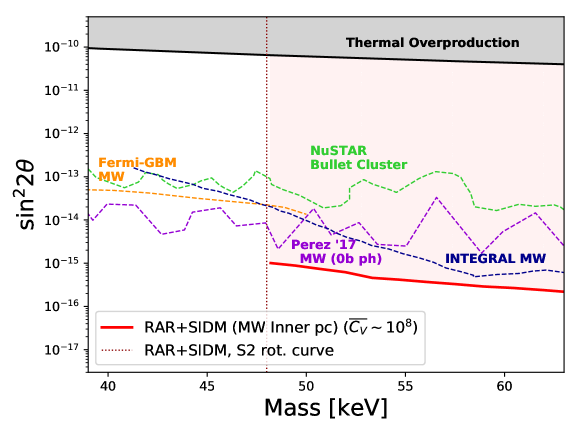
Figure 12: Sterile neutrino parameter space limits obtained for Galactic Center observations using the AMRR profiles (continuous red line) when assuming DM production due to self-interactions through a massive vector field mediator. The light-red shaded region above the continuous red line corresponds to the AMRR limits given by X-ray bounds (i.e. indirect detection analysis), while the vertical shaded region below $48$ keV indicates the smallest DM mass compatible with S-cluster stars’ rotation curve data. The upper shaded region corresponds to production mechanism bounds: non-resonant production under no lepton asymmetry. Other dotted lines refer to several X-ray bounds for different DM halo profiles, including 0-bounce photon analysis. Reprinted from Yunis et al. (2020), Copyright (2020), with permission from Elsevier.

7 Fermionic DM and cosmology

7.1 Formation and stability of fermionic DM halos in a cosmological framework

The formation and stability of collisionless self-gravitating systems are long-standing problems that date back to the work of D. Lynden-Bell in 1967 on violent relaxation and extend to the virialization of DM halos. Such a relaxation process predicts that a Fermi-Dirac phase-space distribution can describe spherical equilibrium states when the extremization of a coarse-grained entropy is reached. In the case of DM fermions, the most general solution develops a degenerate compact core surrounded by a diluted halo. As we have recently shown Argüelles et al. (2018, 2019); Becerra-Vergara et al. (2020), the core-halo profiles obtained within the fermionic DM-RAR model explain the galaxy rotation curves, and the DM core can mimic the effects of a central BH. A yet open problem is whether these astrophysical core-halo configurations can form in nature and if they remain stable within cosmological timescales. These issues have been recently assessed in Argüelles et al. (2021).

Specifically, we performed a thermodynamic stability analysis in the microcanonical ensemble for solutions with given particle numbers at halo virialization in a cosmological framework. For the first time, we demonstrate that the above core-halo DM profiles are stable (i.e., maxima of entropy) and extremely long-lived. We find a critical point at the onset of instability of the core-halo solutions, where the fermion-core collapses towards a supermassive black hole. For particle masses in the keV range, the core-collapse can only occur for $M_{\rm vir}\gtrsim 10^{9}M_{\odot}$ starting at $z_{\rm vir}\approx 10$ in the given cosmological framework. This is a key result since the fermionic DM system can provide a novel mechanism for SMBH formation in the early Universe, offering a possible solution to the yet-open problem of how SMBHs grow so massive so fast. We recall the result of Fig. 13, which evidences the existence of a last stable configuration before the core collapse into an SMBH. We refer the reader to Argüelles et al. (2021) for details on this relevant result.

This thermodynamic approach allows a detailed description of the relaxed halos from the very center to the periphery, which $N$-body simulations do not allow due to finite inner-halo resolution. In addition, it includes richer physical ingredients such as (i) general relativity — necessary for a proper gravitational DM core-collapse to an SMBH; (ii) the quantum nature of the particles — allowing for an explicit fermion mass dependence in the profiles; (iii) the Pauli principle self-consistently included in the phase-space distribution function — giving place to novel core-halo profiles at (violent) relaxation.

Such treatment allows linking the behavior and evolution of the DM particles from the early Universe to the late stages of non-linear structure formation. We obtain the virial halo mass, $M_{\rm vir}$, with associated redshift $z_{\rm vir}$. The fermionic halos are assumed to be formed by fulfilling a maximum entropy production principle at virialization. It allows obtaining a most likely distribution function of Fermi-Dirac type, as first shown in Chavanis (1998) (generalizing Lynden-Bell results), here applied to explain DM halos. Finally, the stability and typical lifetime of such equilibrium states and their possible astrophysical applications are studied with a thermodynamic approach.

For the first time, we have calculated the caloric curves for self-gravitating, tidally-truncated matter distributions of $\mathcal{O}(10)$ keV fermions at finite temperatures within general relativity. We applied this framework to realistic DM halos (i.e., sizes and masses). With the precise shape of the caloric curve, we establish the families of stable as well as astrophysical DM profiles (see Figs. 13 and 14). They are either King-like or develop a core-halo morphology that fits the rotation curve in galaxies (Argüelles et al., 2018, 2019). In the first case, the fermions are in the dilute regime and correspond to a global entropy maximum. In the second case, the degeneracy pressure (i.e., Pauli principle) holds the quantum core against gravity and corresponds to a local entropy maximum. Those metastable states are extremely long-lived, and, as such, they are the more likely to arise in nature. Thus, these results prove that DM halos with a core-halo morphology are a very plausible outcome within nonlinear stages of structure formation.

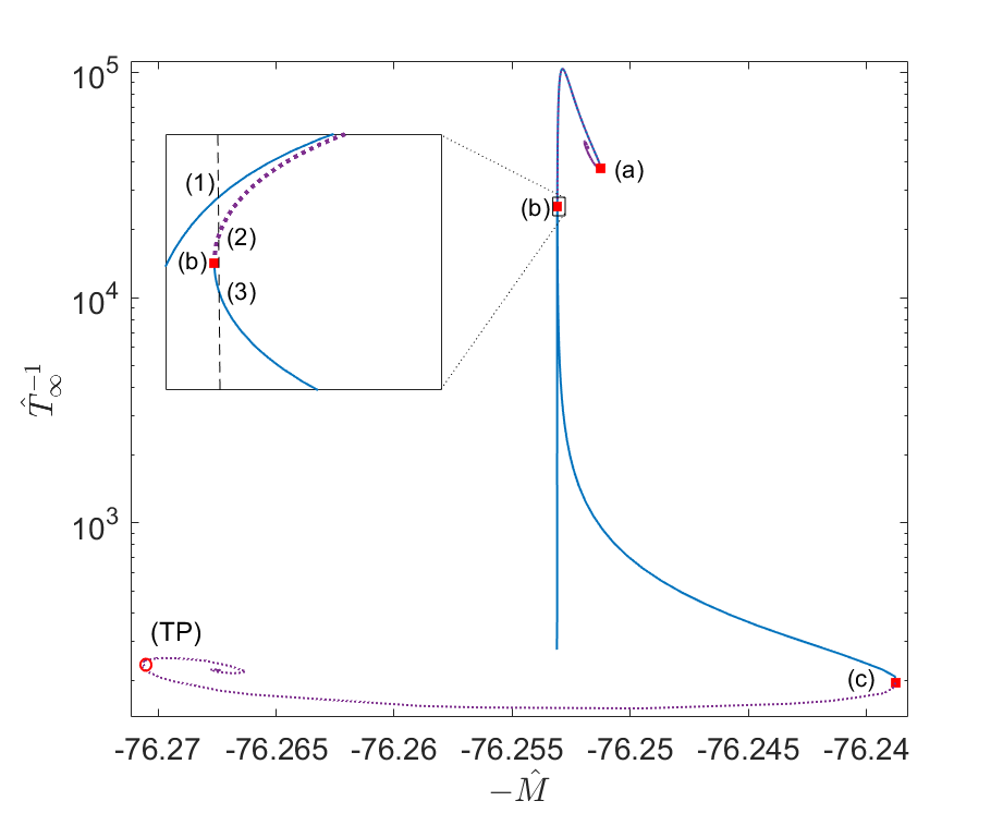
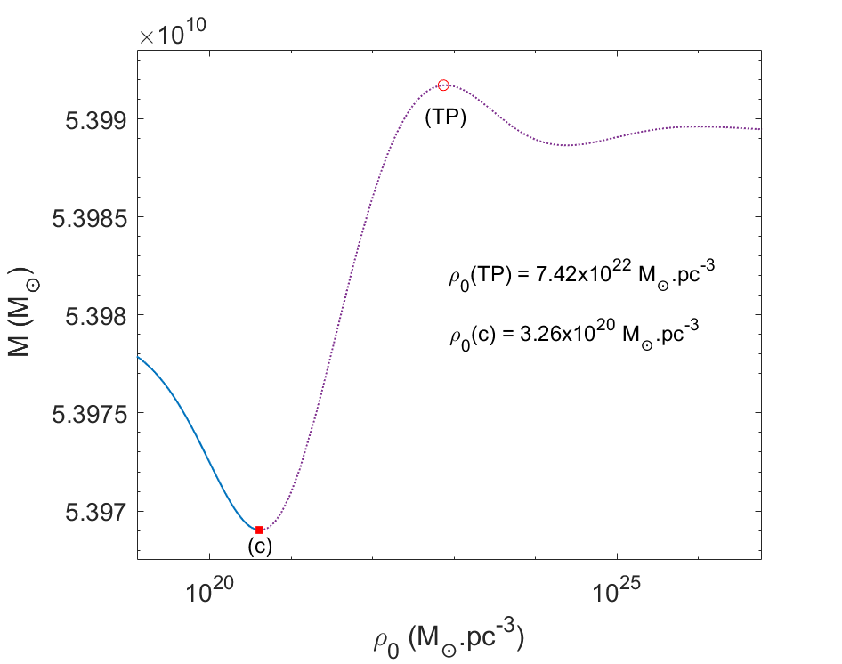
Figure 13: Left: equilibrium solutions along the caloric curve for tidally-truncated configurations of $mc^{2}=48$ keV fermions with fixed $N$. The states within the continuous-blue branches are thermodynamically (and dynamically) stable (i.e., either local or global entropy maxima), while the dotted-violet branches - between (a) and (b) and after (c) - are unstable (i.e., either minimum or saddle point of entropy). Solution (3) is stable and fulfills the virialization conditions. The second spiral of relativistic origin for high $T_{\infty}$ is characteristic of caloric curves at fixed $N$ within general relativity. It implies the existence of a turning point in a mass-central density curve (see right panel). Right: equilibrium states with $N>N_{\rm OV}$ along the $M$ vs. $\rho_{0}$ curve, in correspondence with the caloric curve of the left panel. The last stable configuration at the onset of the core collapse occurs at the minimum of this curve and prior to the turning point instability (corresponding with point (c) in the left panel). Such a critical solution has a core mass $M_{c}^{\rm cr}\approx 2\times 10^{8}M_{\odot}$, thus forming an SMBH from DM core-collapse. Reproduced from Argüelles et al. (2021) with the authors’ permission.

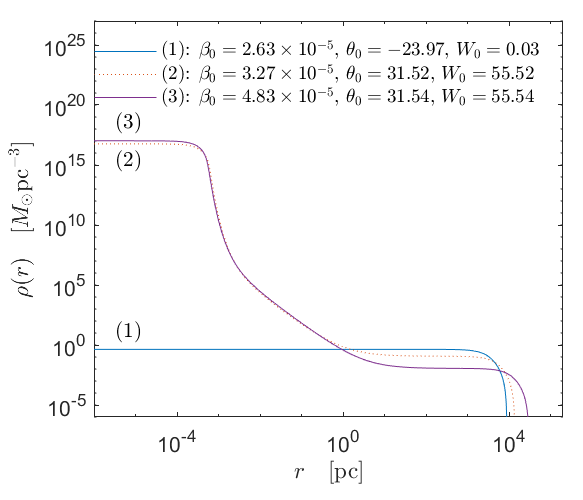
Figure 14: Density profiles for $mc^{2}=48$ keV corresponding with the equilibrium states of the caloric curve in Fig. 13 with corresponding fixed total halo mass. Only profiles (1) (resembling a King distribution) and the core-halo one (3) are stable, while profile (2) is thermodynamically unstable. Interestingly, solutions like (3) were successfully applied to explain the DM halo in the MW in Argüelles et al. (2018). They are stable, extremely long-lived, and fulfill the observed surface DM density relation and the expected value of the DM dispersion velocity. Reproduced from Argüelles et al. (2021) with the authors’ permission.

7.2 Interactions in warm DM: a view from cosmological perturbation theory

The traditional $\Lambda$CDM paradigm of cosmology is in remarkable agreement with large-scale cosmological observations and galaxy properties. However, there are increasing tensions of the $\Lambda$CDM with observations on smaller scales, such as the so-called missing DM sub-halo problem and the core-cusp discrepancy.

High-resolution cosmological simulations of average-sized halos in $\Lambda$CDM predict an overproduction of small-scale structures significantly larger than the observed number of small satellite galaxies in the Local Group. Moreover, $N$-body simulations of CDM predict a cuspy density profile for virialized halos, while observations show dSphs having flattened smooth density profiles in their central regions.

A possible alternative to alleviate or try to resolve such tensions is to consider warm dark matter (WDM) particles, meaning that they are semi-relativistic during the earliest stages of structure formation with non-negligible free-streaming particle length.

WDM models feature an intermediate velocity dispersion between HDM and CDM that results in a suppression of structures at small scales due to free-streaming. If this free streaming scale today is smaller than the size of galaxy clusters, it can solve the missing satellites problem. However, thermally produced WDM suffers from the so-called catch-22 problem when studied within $N$-body simulations Shao et al. (2013). Such WDM-only simulations either show unrealistic core sizes for particle masses above the keV range or acquire the right halo sizes for sub-keV masses in direct conflict with phase-space and Lyman-$\alpha$ constraints.

Another compelling alternative to collisionless CDM, apart from WDM, is to consider interactions in CDM. This consideration relaxes the assumption that CDM interacts only gravitationally after early decoupling and includes interactions between DM and SM particles, additional hidden particles, or among DM particles. These later models are denominated as self-interacting DM models (SIDM).

To shed light on this matter, we have recently provided a general framework for self-interacting WDM in cosmological perturbations by deriving from first principles a Boltzmann hierarchy that retains certain independence from an interaction Lagrangian Yunis et al. (2020). Elastic interactions among the massive particles were considered to obtain a more general hierarchy than those usually obtained for non-relativistic (cold DM) or ultra-relativistic (neutrinos) approximations. The more general momentum-dependent kernel integrals in the Boltzmann collision terms are explicitly calculated for different field-mediator models, including a scalar or massive vector field.

In particular, if the self-interactions maintain the DM fluid in kinetic equilibrium until the fluid becomes non-relativistic, the background distribution function at that moment will switch into a non-relativistic form. This constitutes the scenario known as non-relativistic self-decoupling (a.k.a. late kinetic decoupling). The consequences of this scenario are poorly explored in the literature, and only some preliminary results have been recently obtained within simplified DM fluid approximations Egana-Ugrinovic et al. (2021). However, more recently Yunis et al. (2021), this late kinetic decoupling physics was fully explored with self-interactions treated from first principles using interaction Lagrangian (i.e., superseding the fluid approximation), following the formalism developed in Yunis et al. (2020). There, it was found that if one imposes continuity of the limiting expressions for the energy density, the non-relativistic distribution function can be found in an analytic expression (see Yunis et al. (2021) for details).

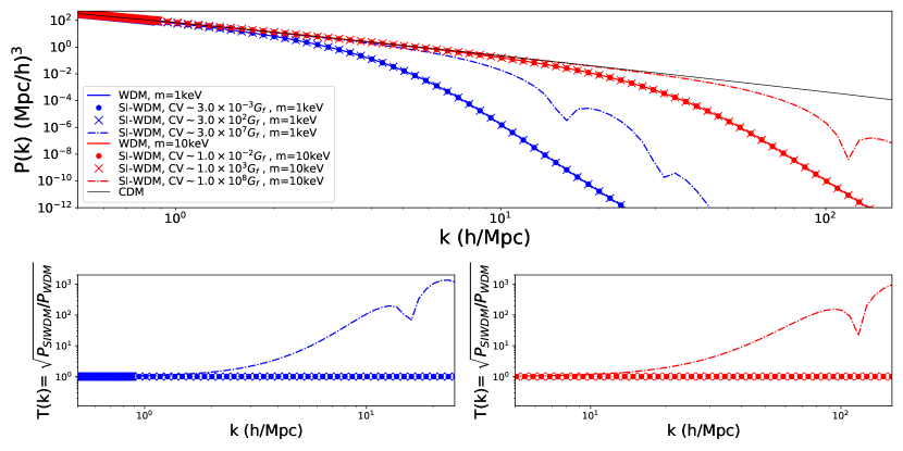
Figure 15: Power Spectrum (top panel) and transfer functions compared to standard WDM (bottom panels) for a vector field SI-WDM model, using a modification to CLASS. We assume the relaxation time approximation and consider two values of the DM particle mass: $1$ and $10$ keV. Also plotted are the power spectra of CDM and WDM models with DM mass of $1$ and $10$ keV. All WDM and SI-WDM models consider a nonresonant production scenario (Dodelson-Widrow mechanism, Dodelson and Widrow (1993)) with $T\sim(4/11)^{1/3}T_{\gamma}$. Importantly, the effect of large enough self-interactions increases the amount of small structure formed for these models (see dot-dashed curves), implying that the few keV (traditional) WDM models which were excluded in the past, can now be back to an agreement with observations in this new SI-WDM scenarios. Reproduced from Yunis et al. (2021), with permission from SNCSC.

Figure 15 illustrates the effects of self-interactions in the matter power spectrum for the case of a massive scalar field-mediator while including the late kinetic decoupling case. We have used an extended version of the CLASS code incorporating our results for SI-WDM with particle masses in the $\sim$ keV range. There, we see some of the particular features of the models. With the inclusion of self-interactions, for models with non-relativistic self-decoupling (i.e., late kinetic decoupling), the resulting power spectra may differ significantly from their relativistic counterparts. Indeed, we find that in this regime, the models are “colder” (i.e., as if they correspond to a higher particle mass) and show, even at smaller $k$ values, a distinctive oscillatory pattern (see, e.g., dot-dashed curves in Fig. 15. This increases the small structures for these models, implying that the few keV (traditional) WDM models excluded from phase-space arguments now agree with observations in this new SI-WDM scenario.

Most tensions inherent to $\nu$MSM WDM models arise from structure formation, i.e., the MW satellite counts and Lyman-$\alpha$ observations: the preferred parameter ranges may underproduce small structures and almost rule out the available parameter space. So, including self-interactions can significantly relax the existing bounds on this family of models. The prediction of these models for the number of MW satellites and the observations of the Lyman-$\alpha$ forest was presented in Yunis et al. (2022) (see Fig. 17).

While in the above paragraphs, we have discussed the effects of self-interacting $\mathcal{O}(1-10)$ keV light fermionic candidates on the linear-structure formation (i.e., its suppression effects on the linear matter power spectrum and its consequences on Lyman-$\alpha$ forest and satellite counts Yunis et al. (2022)), we will discuss in next its effects on DM halo profiles. For this, we will follow the specific self-interacting model where the darkinos are right-handed neutrinos self-interacting via massive (axial) vector-boson mediators (also considered as a possible case in Yunis et al. (2022)). The main consequences of this model for DM halo structures were studied in Yunis et al. (2020), for a particle mass $mc^{2}\approx 50$ keV. In particular, it mainly investigated the consequences of the Milky Way DM halo and the bullet cluster. The massive boson mediator adds a pressure term in the equilibrium equations (see, e.g., Argüelles and et al. (2016); Yunis et al. (2020)) which, for normalized interaction constants up to $\bar{C}_{V}\sim 10^{12}$ (in Fermi constant units), causes no appreciable effects in the Milky Way rotation curve. However, values larger than $\bar{C}_{V}\sim 10^{13}$ are ruled out since the additional pressure term is enough to push forward the halo, spoiling the fit to the data, see Fig. 16. Interestingly, values of interaction strengths between our light fermionic candidates of $\bar{C}_{V}\sim 10^{8}$ agree with the bullet cluster measurements. Indeed, on cluster scales, it was demonstrated in Yunis et al. (2020) (see section 3.2 therein) that such interaction constants resolve the tensions between predictions of $\Lambda$CDM-based numerical simulations and observations since the corresponding self-interacting DM (SIDM) cross section ($\sigma_{SIDM}$) lies in the expected range Harvey et al. (2015)

$$0.1\,\,{\rm cm}^{2}\,{\rm g}^{-1}\leq\frac{\sigma_{\rm SIDM}}{m}\,\leq 0.47\,\,{\rm cm}^{2}\,{\rm g}^{-1}.$$ (11)

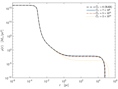
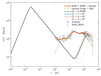
Figure 16: Density profiles (left panel) and rotation curves (right panel) of the extended RAR model with both self-interactions and escape of particle effects. Solutions are shown with four different self-interaction constant values $\bar{C}_{V}$, including the case of $\bar{C}_{V}=0$ in black dashed, corresponding to the original Milky Way fit presented in Argüelles et al. (2018). The model fits the observed total rotation curve data from Sofue (2013) (with error bars). The predicted rotation curve (in solid red) shows the excellent fit to the data for $\bar{C}_{V}=7\times 10^{8}$ (in solid blue) and baryonic components (in green dashed). Notice that the DM halo becomes more extended and less dominant, implying an underfit to the data for large enough $\bar{C}_{V}>10^{13}$, due to the additional pressure term contribution of the boson mediator field. Reprinted from Yunis et al. (2020), Copyright (2020), with permission from Elsevier.

.

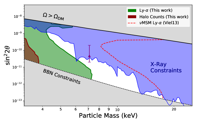
Figure 17: Parameter space constraints for $\nu$MSM, where MW satellite halo counts and Lyman-$\alpha$ forest bounds are analyzed under a self-interacting model as outlined above. For each point $(\theta,m)$ in the parameter space, we consider a self-interacting model under a vector field mediator, with its interaction constant given by $\sigma/m\sim 0.144C_{v}^{2}/m^{3}=0.1$ cm² g^-1, the upper limit given by Bullet Cluster constraints (see Yunis et al. (2022) for details). For comparison, we plot the Lyman-alpha bounds for the non-interacting case for a comparable analysis, plus other bounds to the $\nu$MSM parameter space for informative purposes, namely X-Ray indirect detection bounds (in blue) and sterile neutrino production bounds (in grey). We also plot the sterile neutrino model compatible with a tentative $3.5$ keV DM signal, the subject of debate in recent years, as a purple triangle. The complete list of references of all such bounds can be found in Yunis et al. (2022). Reprinted from Yunis et al. (2022). Copyright IOP Publishing. Reproduced with permission.

8 Additional fermionic DM probes

8.1 Gravitational lensing

Over the last decade, gravitational lensing has become a very effective tool to probe the DM distribution of systems from galaxy to cluster scales. The availability of high-quality HST imaging and integral field spectroscopy with the VLT has allowed high-precision strong lensing models to be developed in recent years, with tight constraints on the inner mass distribution of galaxy clusters (e.g., Bergamini et al. (2019)). By comparing high-resolution mass maps of galaxy cluster cores obtained by such lens models with cosmological hydrodynamical simulations in the LCDM framework, a tension has emerged in the mass profile of the sub-halo population associated with cluster galaxies Meneghetti et al. (2020). Namely, the observed sub-halos appear more compact than those in simulations, with circular velocities inferred from the lens models, which are higher, for a given sub-halo halo mass, than those derived from simulations. It is still unclear whether this tension is due to some limitations of the numerical simulations in the modeling of baryonic physics (back-reaction effects on DM) or rather a more fundamental issue related to the CDM paradigm.

In Gómez et al. (2016), the lensing effects of the core-halo DM distribution were computed. The NFW and nonsingular isothermal sphere (NSIS) DM models and the central Schwarzschild BH model were compared at distances near the Galaxy center. The DM density profiles lead to small deviations of light (of $0.1$ arcsec) in the halo part ($\sim 8$ kpc). However, the RAR profile produces strong lensing effects when the dense core becomes highly compact. For instance, the density distribution of the RAR model for a fermion mass of $\sim 100$ keV generates strong lensing features at distances $\sim 0.1$ mpc (see Gómez et al. (2016) for additional details). The DM quantum core has no photon sphere inside or outside but generates multiple images and Einstein rings. Thus, it will be interesting to compare and contrast lensing images produced by the RAR model with the ones produced by phenomenological profiles.

It is also interesting to construct the shadow-like images produced by the fermion DM cores of the RAR model and analyze them in light of the EHT data from Sgr A*. Indeed, horizonless objects can be compact, lack a hard surface, and cast a shadow surrounded by a ring-like feature of lensed photons Cardoso and Pani (2019). This has been shown for boson stars for Sgr A* in Vincent et al. (2016) and further studied by Olivares et al. (2020) within Numerical Relativity simulations. Using full general relativistic ray tracing techniques Pelle et al. (2022), we have recently computed relativistic images of the fermionic DM cores of the RAR model under the assumption that photons are emitted from a surrounding accretions disc (self-consistently computed in the given metric) and have shown that there exists a particle mass range in which the shadow feature acquires the typical sizes as resolved for the EHT in Sgr A* (Pelle, Argüelles, et al., to be submitted).

8.2 Dynamical friction

The measured orbital period decay of relativistic compact-star binaries (e.g., the famous Hulse-Taylor binary pulsar) has been explained with very-high precision by the gravitational-wave emission predicted by general relativity of an inspiraling binary, assuming the binary is surrounded by empty space and within the point-like approximation of the two bodies. However, the presence of DM around the binary might alter the orbital dynamics because of a traditionally neglected phenomenon: DM dynamical friction (DMDF). The binary components interact with their own gravitational wakes produced by the surrounded DM, leading to an orbital evolution that can be very different from the orbital evolution solely driven by the emission of gravitational waves.

In Pani (2015); Gómez and Rueda (2017), the effect of the DMDF on the motion of NS-NS, NS-WD, and WD-WD was evaluated. Quantitatively, the crucial parameters are the orbital period and the value of the DM density at the binary location in the galaxy. A comparison among the DMDF produced by the NFW, the NSIS, and the RAR model was presented.

For NS-NS, NS-WD, and WD-WD with measured orbital decay rates, the energy loss by gravitational waves dominates over the DMDF effect. However, there are astrophysically viable conditions for which the two effects become comparable. For example, $1.3$–$0.2$ $M_{\odot}$ NS-WD, $1.3$–$1.3$ $M_{\odot}$ NS-NS, and $0.25$–$0.50$ $M_{\odot}$ WD-WD, located at $0.1$ kpc, the two effects compete with each other for a critical orbital period in the range $20$–$30$ days for the NFW model. For the RAR model, it occurs at an orbital period $\sim 100$ days (see Gómez and Rueda (2017) for details). Closer to the Galactic center, the DMDF effect keeps increasing, so the above values for the critical orbital period become shorter. For certain system parameters, the DMDF can lead to an orbital widening rather than a shrinking.

The DMDF depends on the density profile, velocity distribution function, and velocity dispersion profile. Therefore, measuring with high accuracy the orbital decay rate of compact-star binaries at different Galactic locations and as close as possible to the Galactic center might reveal a powerful tool to test DM models.

Indeed, during the peer-reviewing process of this review, Chan and Lee (2023) published an analysis of the DMDF contribution to the orbital decay rate of the X-ray binaries formed by stellar-mass BHs and stellar companions. Specifically, they analyzed the case of A0620–00 and XTE J1118+480, finding that the DMDF can explain their fast orbital decay. The analysis in Chan and Lee (2023) uses a phenomenological DM profile, so it will be interesting to apply the DMDF with the RAR model, as done in Gómez and Rueda (2017), to check whether or not X-ray binaries can further constrain the fermion mass.

8.3 Gravitational collapse of DM cores and SMBH formation

The explanation of the formation, growth, and nature of SMBHs observed at galaxy centers are amongst the most relevant problems in astrophysics and cosmology. Relevant questions yet waiting for an answer are: how can they increase their size in a relatively short time to explain the farthest quasars Volonteri (2012); Woods et al. (2019)?; where do the BH seeds come from and how large they must be to form SMBHs of $\sim 10^{8}$–$10^{9}M_{\odot}$ at high cosmological redshift Zhu et al. (2022)?; and what is the connection between the host galaxy and central SMBH masses Volonteri et al. (2021)?

Scenarios on the origin of SMBHs can be divided according to the formation channel (see Inayoshi et al. (2020); Volonteri et al. (2021) for recent reviews):

1. Channels that advocate a baryonic matter role (gas and stars). (Ia) Population III stars and (Ib) direct collapse to a BH (DCBH). Scenarios (Ia) produce BH seeds $\sim 10^{2}M_{\odot}$ Madau and Rees (2001); Hosokawa et al. (2016), so very-high accretion rates are needed to grow them to $10^{9}M_{\odot}$ in a few billion years. Simulations show that BHs of $<10^{3}M_{\odot}$ cannot grow to $10^{8}M_{\odot}$ at cosmological redshift $z\sim 6$ due to radiative feedback Zhu et al. (2022). DCBH scenarios (Ib) produce BH seeds in the range $10^{4}$–$10^{5}M_{\odot}$ Begelman et al. (2006, 2008); Woods et al. (2017). Hydrodynamic N-body simulations show some preference for DCBH scenarios Zhu et al. (2022); Latif et al. (2022), although numerical and ad-hoc assumptions limit the results generality Zhu et al. (2022).

2. Early Universe channels where BH seeds form before galaxy formation. They include primordial BHs Carr and Kühnel (2020) and exotic candidates like topological defects Bramberger et al. (2015). However, these scenarios are difficult to prove or disprove since those processes are hypothesized to occur in early cosmological epochs not accessed by observations.

Recently, we have proposed in Arguelles et al. (submitted) an SMBH formation channel conceptually different from cases (I) and (II). The new scenario is based on the gravitational collapse and subsequent growth of dense fermionic DM cores. The cores originate at the center of the halos and start to grow as they form. As we have recalled in this work, those dense core-diluted halo DM density distributions are predicted by maximum entropy production principle models of halo formation Argüelles et al. (2021, 2022). We have recalled how the core made of fermions of $\sim 50$ keV rest mass-energy becomes unstable against gravitational collapse into a BH for a threshold mass of $\sim 10^{8}~{}M_{\odot}$. Therefore, the new scenario produces larger BH seeds that comfortably grow to SMBH mass values of $10^{9}M_{\odot}$ in a relatively short time without super-Eddington accretion (Arguelles et al., submitted).

9 Conclusions

Possibly one of the most relevant steps has been to develop a framework that allows obtaining the DM density (and other related physical properties) profiles from first principles. The distribution of DM in the galaxy is given by the solution of the Einstein equations subjected to appropriate boundary conditions to fulfill observational data. The nature of the particle candidate sets the equation of state, so the energy-momentum tensor. It turns out that neutral massive fermion DM particles distribute throughout the galaxy following a dense core-dilute halo density profile. See Section 2 for details.

Thanks to the above, the nature of the DM particle, like the rest mass, can be constrained using stellar dynamics data, e.g., the MW rotational curves data and the most accurate data of the S-cluster stellar orbits around Sgr A*. See Section 3 for details.

A remarkable and intriguing result is that the orbits of the S-stars are correctly described by the presence of the dense core of fermions without the need for the presence of a massive BH at the MW center. We have shown that even the most accurate available data of the S2 star can not distinguish between the two models since both models describe the data with comparable accuracy. However, we have shown that the data of the periapsis precession of the S2 star in the forthcoming three years (i.e., by 2026) could help to discriminate the two scenarios. See Section 3 for details.

In addition to the MW, the RAR model describes the DM component observed in other galaxy types, namely dSphs, ellipticals, and galaxy clusters. This point includes the explanation of existing observational Universal relations and the comparison with other DM models regarding the same observables. See Section 4 for details.

All the above constrains the DM particle nature limiting the fermion mass to the $\sim 50$–$350$ keV range, constituting a relevant starting point for complementary particle physics analyses. Among the plethora of particle-physics candidates, the beyond-standard model sterile neutrinos (also including self-interactions) remain an interesting candidate for being the fermions of the RAR model. See Section 5 for details.

None DM discussion is complete without examining the cosmological implications. In this order of ideas, it has been first shown that the core-halo configurations can indeed form in the Universe in appropriate cosmological timescales thanks to the mechanism of violent relaxation that predicts equilibrium states described by the Fermi-Dirac phase-space distribution. Second, it has been shown that those equilibrium states are long-lasting, with a lifetime of several cosmological timescales, so well over the Universe’s lifetime. Third, it has been shown that those small-scale DM core-halo substructures can form from non-linear cosmological density perturbations during the cosmological evolution. See Section 6 for details.

Last but not least, we have discussed some additional theoretical and observational scenarios that can help to probe DM models. Specifically, if DM permeates galaxies, stellar objects do not sit in a perfect vacuum. Thus, the distribution of DM can cause dynamical friction, a purely gravitational effect that can alter a purely Keplerian motion of binaries, and which, under certain conditions, can become as large as gravitational wave emission losses. Strong gravitational lensing is potentially sensitive to the density profile of DM at sufficiently small scales where DM model profiles differ. We have also outlined how the SMBHs observed at the center of active galaxies can be formed from BH seeds from the gravitational collapse of dense cores of fermionic DM. See Section 6 for details.

In summary, we express that only theoretical models that join microphysics and macrophysics, such as the RAR model, can lead to a comprehensive set of predictions ranging from participle physics to galactic stellar dynamics and to cosmology, which can be put to direct observational scrutiny. We hope that future observations and a further refined analysis of DM models, including the quantum nature of the particles, will lead to a breakthrough in revealing the DM nature.

This research received no external funding.

No new data were created or analyzed in this study. Data sharing is not applicable to this article.

The authors declare no conflict of interest.

yes

Appendix A Equations of motion and effective potential

In general relativity, the Lagrangian for a free particle in a gravitational field can be expressed as

$${\mathcal{L}\left(x^{\alpha},\dfrac{dx^{\alpha}}{d\lambda}\right)=\dfrac{1}{2}g_{\mu\nu}(x^{\alpha})\dfrac{dx^{\mu}}{d\lambda}\dfrac{dx^{\nu}}{d\lambda}\equiv\dfrac{1}{2}g_{\mu\nu}(x^{\alpha})\dot{x}^{\mu}\dot{x}^{\nu}},$$ (12)

where $g_{\mu\nu}$ are the covariant components of the metric tensor, $x^{\beta}$ are the space-time coordinates, and $\lambda$ is an affine parameter. In the space of the curves describe by $\{x^{\mu}(\lambda),\lambda\in[\lambda_{i},\lambda_{f}]\}$, the action is defined as

$$\mathcal{S}=\int\mathcal{L}(x^{\alpha},\dot{x}^{\alpha})d\lambda=\dfrac{1}{2}\int g_{\mu\nu}(x^{\alpha})\dot{x}^{\mu}\dot{x}^{\nu}d\lambda.$$ (13)

The Euler-Lagrange equations are obtained, as usual, by varying the action with respect to the coordinates, and by setting the variation equal to zero. For massive particles, we can change the parameter $\lambda$ by the proper time $\tau$, so by varying a curve

$$x^{\mu}(\tau)\longrightarrow x^{\mu}(\tau)+\delta x^{\mu}(\tau)\ ,$$ (14)

with

$$\delta x^{\mu}(\tau_{i})=\delta x^{\mu}(\tau_{f})=0\ ,$$ (15)

the action variation is

$${\delta\mathcal{S}=\int\left[\dfrac{\partial\mathcal{L}}{\partial x^{\mu}}\delta x^{\mu}+\dfrac{\partial\mathcal{L}}{\partial\dot{x}^{\mu}}\delta(\dot{x}^{\mu})\right]d\tau}.$$ (16)

Since  $\displaystyle{\delta(\dot{x}^{\mu})=\delta(dx^{\mu}/d\tau)=d\delta x^{\mu}/d\tau}$,  the last term in Eq. (16) can be written as

$$\dfrac{\partial\mathcal{L}}{\partial\dot{x}^{\mu}}\delta(\dot{x}^{\mu})=\dfrac{\partial\mathcal{L}}{\partial\dot{x}^{\mu}}\dfrac{d\delta x^{\mu}}{d\tau}=\dfrac{d}{d\tau}\left(\dfrac{\partial\mathcal{L}}{\partial\dot{x}^{\mu}}\delta x^{\mu}\right)-\dfrac{d}{d\tau}\left(\dfrac{\partial\mathcal{L}}{\partial\dot{x}^{\mu}}\right)\delta x^{\mu}.$$ (17)

When integrated between $\tau_{i}$ and $\tau_{f}$ the first term on the right-hand side in the above equation vanishes because  $\delta\dot{x}^{\mu}(\tau_{i})=\delta\dot{x}^{\mu}(\tau_{f})=0$,   therefore, Eq. (16) become

$${\delta\mathcal{S}=\int\left[\dfrac{\partial\mathcal{L}}{\partial x^{\mu}}\delta x^{\mu}-\dfrac{d}{d\tau}\left(\dfrac{\partial\mathcal{L}}{\partial\dot{x}^{\mu}}\right)\delta x^{\mu}\right]d\tau},$$ (18)

so the action variation vanish for all $\delta x^{\mu}$ if, and only if, it is satisfied that

$$\dfrac{\partial\mathcal{L}}{\partial x^{\mu}}-\dfrac{d}{d\tau}\left(\dfrac{\partial\mathcal{L}}{\partial\dot{x}^{\mu}}\right)=0.$$ (19)

For the spherically symmetric metric (6), the Lagrangian of a free particle is

$$\mathcal{L}=\dfrac{1}{2}\left[g_{00}(r)\ \dot{t}^{2}-g_{11}(r)\ \dot{r}^{2}-r^{2}\ \dot{\theta}^{2}-r^{2}\sin^{2}\theta\ \dot{\phi}^{2}\right],$$ (20)

where the dot indicates differentiation with respect to $\tau$, i.e., $\dot{x}^{\mu}=dx^{\mu}/d\tau$. Replacing the Lagrangian, Eq. (20), in the Euler-Lagrange expression, Eq. (19), the equations of motion for $\dot{t}$, $\dot{r}$, $\dot{\theta}$ and $\dot{\phi}$ are

for $\dot{t}$:

$$\dfrac{\partial\mathcal{L}}{\partial t}-\dfrac{d}{d\tau}\left(\dfrac{\partial\mathcal{L}}{\partial\dot{t}}\right)=0\quad\longrightarrow\quad\dfrac{d}{d\tau}\left(g_{00}\dot{t}\right)=0\quad\longrightarrow\quad g_{00}\ \dot{t}=\rm{const}\equiv E,$$

for $\dot{r}$:

$$\dfrac{\partial\mathcal{L}}{\partial r}-\dfrac{d}{d\tau}\left(\dfrac{\partial\mathcal{L}}{\partial\dot{r}}\right)=0 \quad\rightarrow\quad \dfrac{d}{d\tau}\left(-g_{11}\dot{r}\right)-\dfrac{1}{2}(\dot{g}_{00}\dot{t}^{2}-\dot{g}_{11}\dot{r}^{2}-2r\dot{\theta}^{2}-2r\sin^{2}\theta\dot{\phi}^{2})=0$$

$$\quad\rightarrow\quad g_{11}\ \ddot{r}+\dfrac{1}{2}\ \dot{g}_{00}\ \dot{t}^{2}+\dfrac{1}{2}\ \dot{g}_{11}\ \dot{r}^{2}-r\ \dot{\theta}^{2}-r\sin^{2}\theta\ \dot{\phi}^{2}=0,$$

for $\dot{\theta}$:

$$\dfrac{\partial\mathcal{L}}{\partial\theta}-\dfrac{d}{d\tau}\left(\dfrac{\partial\mathcal{L}}{\partial\dot{\theta}}\right)=0 \quad\rightarrow\quad \dfrac{d}{d\tau}\left(-r^{2}\dot{\theta}\right)-(-r^{2}\sin\theta\cos\theta\dot{\phi}^{2})=0$$

$$\quad\rightarrow\quad r^{2}\ \ddot{\theta}+2r\ \dot{\theta}\ \dot{r}-r^{2}\sin\theta\cos\theta\ \dot{\phi}^{2}=0,$$

for $\dot{\phi}$:

$$\dfrac{\partial\mathcal{L}}{\partial\phi}-\dfrac{d}{d\tau}\left(\dfrac{\partial\mathcal{L}}{\partial\dot{\phi}}\right)=0\quad\rightarrow\quad\dfrac{d}{d\tau}\left(-r^{2}\sin^{2}\theta\dot{\phi}\right)=0\ \rightarrow\ r^{2}\sin^{2}\theta\ \dot{\phi}=\rm{const}\equiv L.$$

Due to the spherical symmetry, the metric is invariant under rotations of the polar coordinate. Therefore, we can assume without loss of generality $\theta=\pi/2$. In this case, our set of EOM is the following

$$g_{00}\ \dot{t}=E,$$ (21)

$$g_{11}\ \ddot{r}+\dfrac{1}{2}\ \dot{g}_{00}\ \dot{t}^{2}+\dfrac{1}{2}\ \dot{g}_{11}\ \dot{r}^{2}-r\dot{\phi}^{2}=0,$$ (22)

$$r^{2}\dot{\phi}=L,$$ (23)

where $E$ and $L$ are the conserved energy and the angular momentum of particle per unit mass.

From the condition for mass particle geodesics, $g_{\mu\nu}\dot{x}^{\mu}\dot{x}^{\nu}=1$, and the equation of motion for $t(\tau)$ and $\phi(\tau)$, we can obtain the effective potential. For massive particles must be fulfilled that

$$g_{\mu\nu}\dot{x}^{\mu}\dot{x}^{\nu}=g_{00}(r)\ \dot{t}^{2}-g_{11}(r)\ \dot{r}^{2}-r^{2}\ \dot{\theta}^{2}-r^{2}\sin^{2}\theta\ \dot{\phi}^{2}=1,$$ (24)

so for $\theta=\frac{\pi}{2}$ and replacing Eqs. (21) and (23) in Eq. (24) we obtain

$$g_{00}(r)\ g_{11}(r)\ \dot{r}^{2}=E^{2}-g_{00}(r)\left[1+\left(\dfrac{L}{r}\right)^{2}\right]$$ (25)

where the second term of the right-hand side of the previous equation is the well-known effective potential

$$U^{2}_{eff}(r)\equiv g_{00}(r)\left(1+\dfrac{L^{2}}{r^{2}}\right).$$ (26)

Appendix B Projection of orbit onto the plane of sky

When a telescope measures the motion of a star, it does not measure the real dynamics but rather an apparent one, i.e., it measures the orbit and velocity data projected on the plane that lies perpendicular to the line of sight of the star. For this reason, to compare the theoretical orbit with the observational data, we must project the real orbit on the observation plane in the sky as shown in Fig. 18. This plane-of-sky is described in coordinates $(X,Y)$ defined by the observed angular positions (the declination $\delta$ and the right ascension $\alpha$), where $X=R_{\odot}(\delta-\delta_{\rm SgrA*})$ and $Y=R_{\odot}(\alpha-\alpha_{\rm SgrA*})$ being $R_{\odot}$ the distance to the Galactic center Ghez et al. (2008); Chu et al. (2018); Do et al. (2019). According to the above description, the apparent theoretical orbit can then be obtained from:

$$X = x\ \cos(X,x)+y\ \cos(X,y),$$ (27)

$$Y = x\ \cos(Y,x)+y\ \cos(Y,y),$$ (28)

where the coordinates $(x,y)$ are determined in the plane of the orbit from $x=r\cos\phi$ and $y=r\sin\phi$, while the direction cosines can be found by Eulerian rotation of axes, this is:

$$\left(\begin{matrix}X\\ Y\\ Z\\ \end{matrix}\right)=\left(\begin{matrix}\cos\Omega&-\sin\Omega&0\\ \sin\Omega&\cos\Omega&0\\ 0&0&1\\ \end{matrix}\right)\left(\begin{matrix}1&0&0\\ 0&\cos i&-\sin i\\ 0&\sin i&\cos i\\ \end{matrix}\right)\left(\begin{matrix}\cos\omega&-\sin\omega&0\\ \sin\omega&\cos\omega&0\\ 0&0&1\\ \end{matrix}\right)\left(\begin{matrix}x\\ y\\ z\\ \end{matrix}\right),$$

$$\left(\begin{matrix}X\\ Y\\ Z\\ \end{matrix}\right)=\left(\begin{array}[]{ccc}\cos\omega\cos\Omega-\cos i\sin\omega\sin\Omega&-\sin\omega\cos\Omega-\cos i\cos\omega\sin\Omega&\sin i\sin\Omega\\ \cos i\sin\omega\cos\Omega+\cos\omega\sin\Omega&\cos i\cos\omega\cos\Omega-\sin\omega\sin\Omega&-\sin i\cos\Omega\\ \sin i\sin\omega&\sin i\cos\omega&\cos i\\ \end{array}\right)\left(\begin{matrix}x\\ y\\ z\\ \end{matrix}\right),$$

being

$$\cos(X,x) = \cos\Omega\cos\omega-\sin\Omega\sin\omega\cos i,$$ (29)

$$\cos(X,y) = -\cos\Omega\sin\omega-\sin\Omega\cos\omega\cos i,$$ (30)

$$\cos(Y,x) = \sin\Omega\cos\omega+\cos\Omega\sin\omega\cos i,$$ (31)

$$\cos(Y,y) = -\sin\Omega\sin\omega+\cos\Omega\cos\omega\cos i,$$ (32)

finally we find that orbit on plane-of-sky is given by:

$$X = r\left[\cos(\phi+\omega)\cos\Omega-\sin(\phi+\omega)\sin\Omega\cos i\right],$$ (33)

$$Y = r\left[\cos(\phi+\omega)\sin\Omega+\sin(\phi+\omega)\cos\Omega\cos i\right].$$ (34)

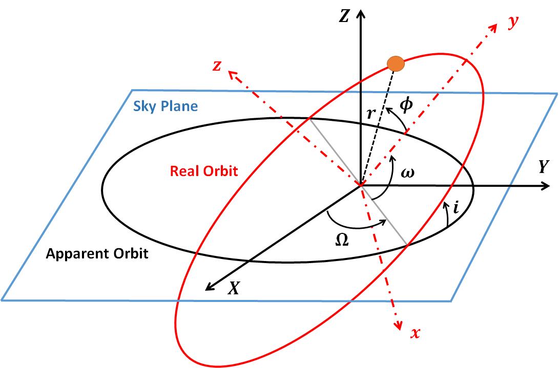
Figure 18: Projection of the real orbit onto the plane of the sky. The axes originate at Sgr A* (the focus of the ellipse). The picture illustrates the orbital parameters: $\phi$ is the azimuth angle of the spherical system of coordinates associated with the $x$, $y$, $z$ Cartesian coordinates, i.e., for an elliptic motion in the $x$-$y$ plane, it is the true anomaly, $i$ is the angle of inclination between the real orbit and the observation plane, $\Omega$ is the angle of the ascending node, and $\omega$ is the argument of pericenter. It is worth noting that the $Z$-axis of the coordinate system is defined by the vector pointing from the Solar System to the Galactic center. Reproduced from Becerra-Vergara et al. (2020) with permission from Astronomy & Astrophysics, Copyright ESO.

Similarly to orbit, the star’s radial velocity must also be projected onto the plane of the sky. The radial velocity on the observation plane is defined as the velocity in the observer’s direction along the line of sight. Therefore, if we adopt the $X$-$Y$ plane as the observation plane, then the line of sight is in the direction of the $Z$-axis given by

$$Z\ =\ x\ \cos(Z,x)+y\ \cos(Z,y),$$ (35)

where

$$\cos(Z,x) = \sin\omega\sin i,$$ (36)

$$\cos(Z,y) = \cos\omega\sin i,$$ (37)

in terms of $\phi,\omega$ and $i$; $Z$ is given by

$$Z=r\sin(\phi+\omega)\sin i.$$ (38)

The radial velocity is defined as the velocity along the observer’s line of sight, and since $Z$ is the direction along the observer’s line of sight, the derivative of $Z$ relative to time gives us the apparent radial velocity of the star. This is

$$\frac{dZ}{dt}=u_{Z}=\left[r\dot{\phi}\ \cos(\phi+\omega)+\dot{r}\ \sin(\phi+\omega)\right]\sin(i).$$ (39)

It is worth noting that in the coordinate system $(X,Y,Z)$, the direction of $Z$-axis is defined by the vector pointing from the Solar System to the Galactic center and that the axes originate at Sgr A*, which is considered the focus of the orbit Gillessen et al. (2017); Gravity Collaboration et al. (2018); Do et al. (2019).

References

References

- Bond et al. (1980) Bond, J.R.; Efstathiou, G.; Silk, J. Massive Neutrinos and the Large-Scale Structure of the Universe. Phys. Rev. Lett. 1980, 45, 1980–1984. https://doi.org/10.1103/PhysRevLett.45.1980.
- Hut and White (1984) Hut, P.; White, S.D.M. Can a neutrino-dominated Universe be rejected? Nature 1984, 310, 637–640. https://doi.org/10.1038/310637a0.
- Alcock et al. (2000) Alcock, C.; Allsman, R.A.; Alves, D.R.; Axelrod, T.S.; Becker, A.C.; Bennett, D.P.; Cook, K.H.; Dalal, N.; Drake, A.J.; Freeman, K.C.; et al. The MACHO Project: Microlensing Results from 5.7 Years of Large Magellanic Cloud Observations. ApJ 2000, 542, 281–307, [arXiv:astro-ph/astro-ph/0001272]. https://doi.org/10.1086/309512.
- Bertone et al. (2005) Bertone, G.; Hooper, D.; Silk, J. Particle dark matter: evidence, candidates and constraints. Phys. Rep. 2005, 405, 279–390, [arXiv:hep-ph/hep-ph/0404175]. https://doi.org/10.1016/j.physrep.2004.08.031.
- Bertone and Tait (2018) Bertone, G.; Tait, T.M.P. A new era in the search for dark matter. Nature 2018, 562, 51–56, [arXiv:astro-ph.CO/1810.01668]. https://doi.org/10.1038/s41586-018-0542-z.
- Bahcall et al. (1999) Bahcall, N.A.; Ostriker, J.P.; Perlmutter, S.; Steinhardt, P.J. The Cosmic Triangle: Revealing the State of the Universe. Science 1999, 284, 1481, [arXiv:astro-ph/astro-ph/9906463]. https://doi.org/10.1126/science.284.5419.1481.
- Ivanov et al. (2020) Ivanov, M.M.; Simonović, M.; Zaldarriaga, M. Cosmological parameters and neutrino masses from the final P l a n c k and full-shape BOSS data. Phys. Rev. D 2020, 101, 083504, [arXiv:astro-ph.CO/1912.08208]. https://doi.org/10.1103/PhysRevD.101.083504.
- Marsh (2016) Marsh, D.J.E. Axion cosmology. Phys. Rep. 2016, 643, 1–79, [arXiv:astro-ph.CO/1510.07633]. https://doi.org/10.1016/j.physrep.2016.06.005.
- Adhikari et al. (2017) Adhikari, R.; Agostini, M.; Ky, N.A.; Araki, T.; Archidiacono, M.; Bahr, M.; Baur, J.; Behrens, J.; Bezrukov, F.; Bhupal Dev, P.S.; et al. A White Paper on keV sterile neutrino Dark Matter. JCAP 2017, 2017, 025, [arXiv:hep-ph/1602.04816]. https://doi.org/10.1088/1475-7516/2017/01/025.
- Schive et al. (2014) Schive, H.Y.; Chiueh, T.; Broadhurst, T. Cosmic structure as the quantum interference of a coherent dark wave. Nature Physics 2014, 10, 496–499, [arXiv:astro-ph.GA/1406.6586]. https://doi.org/10.1038/nphys2996.
- Argüelles et al. (2021) Argüelles, C.R.; Díaz, M.I.; Krut, A.; Yunis, R. On the formation and stability of fermionic dark matter haloes in a cosmological framework. MNRAS 2021, 502, 4227–4246, [arXiv:astro-ph.GA/2012.11709]. https://doi.org/10.1093/mnras/staa3986.
- Suárez and Chavanis (2017) Suárez, A.; Chavanis, P.H. Cosmological evolution of a complex scalar field with repulsive or attractive self-interaction. Phys. Rev. D 2017, 95, 063515, [arXiv:gr-qc/1608.08624]. https://doi.org/10.1103/PhysRevD.95.063515.
- Chavanis (2021) Chavanis, P.H. Jeans mass-radius relation of self-gravitating Bose-Einstein condensates and typical parameters of the dark matter particle. Phys. Rev. D 2021, 103, 123551, [arXiv:gr-qc/2011.01038]. https://doi.org/10.1103/PhysRevD.103.123551.
- Ruffini and Bonazzola (1969) Ruffini, R.; Bonazzola, S. Systems of Self-Gravitating Particles in General Relativity and the Concept of an Equation of State. Physical Review 1969, 187, 1767–1783. https://doi.org/10.1103/PhysRev.187.1767.
- Baldeschi et al. (1983) Baldeschi, M.R.; Gelmini, G.B.; Ruffini, R. On massive fermions and bosons in galactic halos. Physics Letters B 1983, 122, 221–224. https://doi.org/10.1016/0370-2693(83)90688-3.
- Sin (1994) Sin, S.J. Late-time phase transition and the galactic halo as a Bose liquid. Phys. Rev. D 1994, 50, 3650–3654, [arXiv:hep-ph/hep-ph/9205208]. https://doi.org/10.1103/PhysRevD.50.3650.
- Hu et al. (2000) Hu, W.; Barkana, R.; Gruzinov, A. Fuzzy Cold Dark Matter: The Wave Properties of Ultralight Particles. Phys. Rev. Lett. 2000, 85, 1158–1161, [arXiv:astro-ph/astro-ph/0003365]. https://doi.org/10.1103/PhysRevLett.85.1158.
- Matos and Arturo Ureña-López (2001) Matos, T.; Arturo Ureña-López, L. Further analysis of a cosmological model with quintessence and scalar dark matter. Phys. Rev. D 2001, 63, 063506, [arXiv:astro-ph/astro-ph/0006024]. https://doi.org/10.1103/PhysRevD.63.063506.
- Robles and Matos (2012) Robles, V.H.; Matos, T. Flat central density profile and constant dark matter surface density in galaxies from scalar field dark matter. MNRAS 2012, 422, 282–289, [arXiv:astro-ph.CO/1201.3032]. https://doi.org/10.1111/j.1365-2966.2012.20603.x.
- Hui et al. (2017) Hui, L.; Ostriker, J.P.; Tremaine, S.; Witten, E. Ultralight scalars as cosmological dark matter. Phys. Rev. D 2017, 95, 043541, [arXiv:astro-ph.CO/1610.08297]. https://doi.org/10.1103/PhysRevD.95.043541.
- Bar et al. (2018) Bar, N.; Blas, D.; Blum, K.; Sibiryakov, S. Galactic rotation curves versus ultralight dark matter: Implications of the soliton-host halo relation. Phys. Rev. D 2018, 98, 083027, [arXiv:astro-ph.CO/1805.00122]. https://doi.org/10.1103/PhysRevD.98.083027.
- Mocz et al. (2020) Mocz, P.; Fialkov, A.; Vogelsberger, M.; Becerra, F.; Shen, X.; Robles, V.H.; Amin, M.A.; Zavala, J.; Boylan-Kolchin, M.; Bose, S.; et al. Galaxy formation with BECDM - II. Cosmic filaments and first galaxies. MNRAS 2020, 494, 2027–2044, [arXiv:astro-ph.CO/1911.05746]. https://doi.org/10.1093/mnras/staa738.
- Destri et al. (2013) Destri, C.; de Vega, H.J.; Sanchez, N.G. Fermionic warm dark matter produces galaxy cores in the observed scales because of quantum mechanics. New Astronomy 2013, 22, 39–50, [arXiv:astro-ph.CO/1204.3090]. https://doi.org/10.1016/j.newast.2012.12.003.
- Domcke and Urbano (2015) Domcke, V.; Urbano, A. Dwarf spheroidal galaxies as degenerate gas of free fermions. JCAP 2015, 2015, 002–002, [arXiv:hep-ph/1409.3167]. https://doi.org/10.1088/1475-7516/2015/01/002.
- Randall et al. (2017) Randall, L.; Scholtz, J.; Unwin, J. Cores in Dwarf Galaxies from Fermi Repulsion. MNRAS 2017, 467, 1515–1525, [arXiv:astro-ph.GA/1611.04590]. https://doi.org/10.1093/mnras/stx161.
- Chavanis (2022) Chavanis, P.H. Predictive model of fermionic dark matter halos with a quantum core and an isothermal atmosphere. Phys. Rev. D 2022, 106, 043538, [arXiv:gr-qc/2112.07726]. https://doi.org/10.1103/PhysRevD.106.043538.
- de Vega et al. (2014) de Vega, H.J.; Salucci, P.; Sanchez, N.G. Observational rotation curves and density profiles versus the Thomas-Fermi galaxy structure theory. MNRAS 2014, 442, 2717–2727, [arXiv:astro-ph.CO/1309.2290]. https://doi.org/10.1093/mnras/stu972.
- Gao et al. (1990) Gao, J.G.; Merafina, M.; Ruffini, R. The semidegenerate configurations of a selfgravitating system of fermions. A&A 1990, 235, 1–7.
- Chavanis (1998) Chavanis, P.H. On the ‘coarse-grained’ evolution of collisionless stellar systems. MNRAS 1998, 300, 981–991. https://doi.org/10.1046/j.1365-8711.1998.01867.x.
- Bilic et al. (2002) Bilic, N.; Munyaneza, F.; Tupper, G.B.; Viollier, R.D. The dynamics of stars near Sgr A* and dark matter at the center and in the halo of the Galaxy. Progress in Particle and Nuclear Physics 2002, 48, 291–300. https://doi.org/10.1016/S0146-6410(02)00136-9.
- Chavanis et al. (2015) Chavanis, P.H.; Lemou, M.; Méhats, F. Models of dark matter halos based on statistical mechanics: The fermionic King model. Phys. Rev. D 2015, 92, 123527, [arXiv:astro-ph.CO/1409.7840]. https://doi.org/10.1103/PhysRevD.92.123527.
- Argüelles et al. (2018) Argüelles, C.R.; Krut, A.; Rueda, J.A.; Ruffini, R. Novel constraints on fermionic dark matter from galactic observables I: The Milky Way. Physics of the Dark Universe 2018, 21, 82, [arXiv:astro-ph.GA/1606.07040]. https://doi.org/10.1016/j.dark.2018.07.002.
- Argüelles et al. (2019) Argüelles, C.R.; Krut, A.; Rueda, J.A.; Ruffini, R. Novel constraints on fermionic dark matter from galactic observables II: Galaxy scaling relations. Phys. Dark Universe 2019, 24, 100278. https://doi.org/10.1016/j.dark.2019.100278.
- Becerra-Vergara et al. (2020) Becerra-Vergara, E.A.; Argüelles, C.R.; Krut, A.; Rueda, J.A.; Ruffini, R. Geodesic motion of S2 and G2 as a test of the fermionic dark matter nature of our Galactic core. A&A 2020, 641, A34, [arXiv:astro-ph.GA/2007.11478]. https://doi.org/10.1051/0004-6361/201935990.
- Becerra-Vergara et al. (2021) Becerra-Vergara, E.A.; Argüelles, C.R.; Krut, A.; Rueda, J.A.; Ruffini, R. Hinting a dark matter nature of Sgr A* via the S-stars. MNRAS 2021, 505, L64–L68, [arXiv:astro-ph.GA/2105.06301]. https://doi.org/10.1093/mnrasl/slab051.
- Argüelles et al. (2022) Argüelles, C.R.; Mestre, M.F.; Becerra-Vergara, E.A.; Crespi, V.; Krut, A.; Rueda, J.A.; Ruffini, R. What does lie at the Milky Way centre? Insights from the S2-star orbit precession. MNRAS 2022, 511, L35–L39, [arXiv:astro-ph.GA/2109.10729]. https://doi.org/10.1093/mnrasl/slab126.
- Argüelles et al. (2023) Argüelles, C.R.; Krut, A.; Rueda, J.A.; Ruffini, R. Galaxy Rotation Curves and Universal Scaling Relations: Comparison between Phenomenological and Fermionic Dark Matter Profiles. ApJ 2023, 945, 1. https://doi.org/10.3847/1538-4357/acb8bd.
- Ruffini et al. (2015) Ruffini, R.; Argüelles, C.R.; Rueda, J.A. On the core-halo distribution of dark matter in galaxies. Mon. Not. R. Astron. Soc. 2015, 451, 622–628, [1409.7365]. https://doi.org/10.1093/mnras/stv1016.
- Siutsou et al. (2015) Siutsou, I.; Argüelles, C.R.; Ruffini, R. Dark matter massive fermions and Einasto profiles in galactic haloes. Astronomy Reports 2015, 59, 656–666, [arXiv:astro-ph.GA/1402.0695]. https://doi.org/10.1134/S1063772915070124.
- Argüelles and et al. (2016) Argüelles, C.R.; et al.. The role of self-interacting right-handed neutrinos in galactic structure. J. Cosmol. Astropart. Phys. 2016, 4, 038, [1502.00136]. https://doi.org/10.1088/1475-7516/2016/04/038.
- Mavromatos et al. (2017) Mavromatos, N.E.; Argüelles, C.R.; Ruffini, R.; Rueda, J.A. Self-interacting dark matter. International Journal of Modern Physics D 2017, 26, 1730007. https://doi.org/10.1142/S0218271817300075.
- Tolman (1930) Tolman, R.C. On the Weight of Heat and Thermal Equilibrium in General Relativity. Phys. Rev. 1930, 35, 904–924. https://doi.org/10.1103/PhysRev.35.904.
- Klein (1949) Klein, O. On the Thermodynamical Equilibrium of Fluids in Gravitational Fields. Rev. Mod. Phys. 1949, 21, 531–533. https://doi.org/10.1103/RevModPhys.21.531.
- Merafina and Ruffini (1989) Merafina, M.; Ruffini, R. Systems of selfgravitating classical particles with a cutoff in their distribution function. Astron. & Astrophys. 1989, 221, 4–19.
- Sofue (2013) Sofue, Y. Rotation Curve and Mass Distribution in the Galactic Center - From Black Hole to Entire Galaxy. Publ. Astron. Soc. Jpn. 2013, 65, 118, [1307.8241]. https://doi.org/10.1093/pasj/65.6.118.
- Gillessen et al. (2017) Gillessen, S.; Plewa, P.M.; Eisenhauer, F.; Sari, R.; Waisberg, I.; Habibi, M.; Pfuhl, O.; George, E.; Dexter, J.; von Fellenberg, S.; et al. An Update on Monitoring Stellar Orbits in the Galactic Center. ApJ 2017, 837, 30, [arXiv:astro-ph.GA/1611.09144]. https://doi.org/10.3847/1538-4357/aa5c41.
- Gillessen et al. (2009) Gillessen, S.; Eisenhauer, F.; Fritz, T.K.; Bartko, H.; Dodds-Eden, K.; Pfuhl, O.; Ott, T.; Genzel, R. The Orbit of the Star S2 Around SGR A* from Very Large Telescope and Keck Data. Astrophys. J. 2009, 707, L114–L117, [0910.3069]. https://doi.org/10.1088/0004-637X/707/2/L114.
- Argüelles and Ruffini (2014) Argüelles, C.R.; Ruffini, R. Are the most super-massive dark compact objects harbored at the center of dark matter halos? International Journal of Modern Physics D 2014, 23, 1442020, [arXiv:astro-ph.GA/1405.7505]. https://doi.org/10.1142/S0218271814420206.
- Argüelles et al. (2014) Argüelles, C.R.; Ruffini, R.; Fraga, B.M.O. Critical configurations for a system of semidegenerate fermions. Journal of Korean Physical Society 2014, 65, 809–813, [arXiv:astro-ph.GA/1402.1329]. https://doi.org/10.3938/jkps.65.809.
- Argüelles et al. (2019) Argüelles, C.R.; Krut, A.; Rueda, J.A.; Ruffini, R. Can fermionic dark matter mimic supermassive black holes? International Journal of Modern Physics D 2019, 28, 1943003, [arXiv:astro-ph.GA/1905.09776]. https://doi.org/10.1142/S021827181943003X.
- Argüelles et al. (2021) Argüelles, C.R.; Mestre, M.F.; Becerra-Vergara, E.A.; Crespi, V.; Krut, A.; Rueda, J.A.; Ruffini, R. What does lie at the Milky Way centre? Insights from the S2 star orbit precession. MNRAS 2021, [arXiv:astro-ph.GA/2109.10729]. https://doi.org/10.1093/mnrasl/slab126.
- Gravity Collaboration et al. (2018) Gravity Collaboration.; Abuter, R.; Amorim, A.; Anugu, N.; Bauböck, M.; Benisty, M.; Berger, J.P.; Blind, N.; Bonnet, H.; Brandner, W.; et al. Detection of the gravitational redshift in the orbit of the star S2 near the Galactic centre massive black hole. Astron. Astrophys. 2018, 615, L15, [1807.09409]. https://doi.org/10.1051/0004-6361/201833718.
- Zakharov (2022) Zakharov, A.F. Testing the Galactic Centre potential with S-stars. MNRAS 2022, 513, L6–L9, [arXiv:astro-ph.GA/2108.09709]. https://doi.org/10.1093/mnrasl/slab111.
- Gravity Collaboration et al. (2018) Gravity Collaboration.; Abuter, R.; Amorim, A.; Bauböck, M.; Berger, J.P.; Bonnet, H.; Brandner, W.; Clénet, Y.; Coudé Du Foresto, V.; de Zeeuw, P.T.; et al. Detection of orbital motions near the last stable circular orbit of the massive black hole SgrA*. Astron. & Astrophys. 2018, 618, L10, [1810.12641]. https://doi.org/10.1051/0004-6361/201834294.
- Matsumoto et al. (2020) Matsumoto, T.; Chan, C.H.; Piran, T. The origin of hotspots around Sgr A*: orbital or pattern motion? MNRAS 2020, 497, 2385–2392, [arXiv:astro-ph.HE/2004.13029]. https://doi.org/10.1093/mnras/staa2095.
- Peißker et al. (2020a) Peißker, F.; Eckart, A.; Parsa, M. S62 on a 9.9 yr Orbit around SgrA*. ApJ 2020, 889, 61, [arXiv:astro-ph.GA/2002.02341]. https://doi.org/10.3847/1538-4357/ab5afd.
- Peißker et al. (2020b) Peißker, F.; Eckart, A.; Zajaček, M.; Ali, B.; Parsa, M. S62 and S4711: Indications of a Population of Faint Fast-moving Stars inside the S2 Orbit—S4711 on a 7.6 yr Orbit around Sgr A*. ApJ 2020, 899, 50, [arXiv:astro-ph.GA/2008.04764]. https://doi.org/10.3847/1538-4357/ab9c1c.
- GRAVITY Collaboration et al. (2020) GRAVITY Collaboration.; Abuter, R.; Amorim, A.; Bauböck, M.; Berger, J.P.; Bonnet, H.; Brandner, W.; Cardoso, V.; Clénet, Y.; de Zeeuw, P.T.; et al. Detection of the Schwarzschild precession in the orbit of the star S2 near the Galactic centre massive black hole. A&A 2020, 636, L5, [arXiv:astro-ph.GA/2004.07187]. https://doi.org/10.1051/0004-6361/202037813.
- Do et al. (2019) Do, T.; Hees, A.; Ghez, A.; Martinez, G.D.; Chu, D.S.; Jia, S.; Sakai, S.; Lu, J.R.; Gautam, A.K.; O’Neil, K.K.; et al. Relativistic redshift of the star S0-2 orbiting the Galactic Center supermassive black hole. Science 2019, 365, 664–668, [arXiv:astro-ph.GA/1907.10731]. https://doi.org/10.1126/science.aav8137.
- Walker et al. (2009) Walker, M.G.; Mateo, M.; Olszewski, E.W.; Peñarrubia, J.; Evans, N.W.; Gilmore, G. A Universal Mass Profile for Dwarf Spheroidal Galaxies? ApJ 2009, 704, 1274–1287, [arXiv:astro-ph.CO/0906.0341]. https://doi.org/10.1088/0004-637X/704/2/1274.
- de Blok et al. (2008) de Blok, W.J.G.; Walter, F.; Brinks, E.; Trachternach, C.; Oh, S.H.; Kennicutt, R. C., J. High-Resolution Rotation Curves and Galaxy Mass Models from THINGS. AJ 2008, 136, 2648–2719, [arXiv:astro-ph/0810.2100]. https://doi.org/10.1088/0004-6256/136/6/2648.
- Hoekstra et al. (2005) Hoekstra, H.; Hsieh, B.C.; Yee, H.K.C.; Lin, H.; Gladders, M.D. Virial Masses and the Baryon Fraction in Galaxies. ApJ 2005, 635, 73–85, [arXiv:astro-ph/astro-ph/0510097]. https://doi.org/10.1086/496913.
- Donato et al. (2009) Donato, F.; Gentile, G.; Salucci, P.; Frigerio Martins, C.; Wilkinson, M.I.; Gilmore, G.; Grebel, E.K.; Koch, A.; Wyse, R. A constant dark matter halo surface density in galaxies. MNRAS 2009, 397, 1169–1176, [arXiv:astro-ph.CO/0904.4054]. https://doi.org/10.1111/j.1365-2966.2009.15004.x.
- Romanowsky and Kochanek (2001) Romanowsky, A.J.; Kochanek, C.S. Dynamics of Stars and Globular Clusters in M87. ApJ 2001, 553, 722–732, [arXiv:astro-ph/astro-ph/0008062]. https://doi.org/10.1086/320947.
- Newman et al. (2013) Newman, A.B.; Treu, T.; Ellis, R.S.; Sand, D.J. The Density Profiles of Massive, Relaxed Galaxy Clusters. II. Separating Luminous and Dark Matter in Cluster Cores. ApJ 2013, 765, 25, [arXiv:astro-ph.CO/1209.1392]. https://doi.org/10.1088/0004-637X/765/1/25.
- Zhao (1996) Zhao, H. Analytical models for galactic nuclei. MNRAS 1996, 278, 488–496, [astro-ph/9509122]. https://doi.org/10.1093/mnras/278.2.488.
- McGaugh et al. (2016) McGaugh, S.S.; Lelli, F.; Schombert, J.M. Radial Acceleration Relation in Rotationally Supported Galaxies. Phys. Rev. Lett. 2016, 117, 201101, [arXiv:astro-ph.GA/1609.05917]. https://doi.org/10.1103/PhysRevLett.117.201101.
- McGaugh (2004) McGaugh, S.S. The Mass Discrepancy-Acceleration Relation: Disk Mass and the Dark Matter Distribution. ApJ 2004, 609, 652–666, [arXiv:astro-ph/astro-ph/0403610]. https://doi.org/10.1086/421338.
- Ferrarese (2002) Ferrarese, L. Beyond the Bulge: A Fundamental Relation between Supermassive Black Holes and Dark Matter Halos. ApJ 2002, 578, 90–97, [arXiv:astro-ph/astro-ph/0203469]. https://doi.org/10.1086/342308.
- Bogdán and Goulding (2015) Bogdán, Á.; Goulding, A.D. Connecting Dark Matter Halos with the Galaxy Center and the Supermassive Black Hole. ApJ 2015, 800, 124, [1502.05043]. https://doi.org/10.1088/0004-637X/800/2/124.
- Kormendy and Bender (2011) Kormendy, J.; Bender, R. Supermassive black holes do not correlate with dark matter haloes of galaxies. Nature 2011, 469, 377–380, [1101.4650]. https://doi.org/10.1038/nature09695.
- Seth et al. (2014) Seth, A.C.; van den Bosch, R.; Mieske, S.; Baumgardt, H.; Brok, M.D.; Strader, J.; Neumayer, N.; Chilingarian, I.; Hilker, M.; McDermid, R.; et al. A supermassive black hole in an ultra-compact dwarf galaxy. Nature 2014, 513, 398–400, [arXiv:astro-ph.GA/1409.4769]. https://doi.org/10.1038/nature13762.
- Ahn et al. (2017) Ahn, C.P.; Seth, A.C.; den Brok, M.; Strader, J.; Baumgardt, H.; van den Bosch, R.; Chilingarian, I.; Frank, M.; Hilker, M.; McDermid, R.; et al. Detection of Supermassive Black Holes in Two Virgo Ultracompact Dwarf Galaxies. ApJ 2017, 839, 72, [arXiv:astro-ph.GA/1703.09221]. https://doi.org/10.3847/1538-4357/aa6972.
- Afanasiev et al. (2018) Afanasiev, A.V.; Chilingarian, I.V.; Mieske, S.; Voggel, K.T.; Picotti, A.; Hilker, M.; Seth, A.; Neumayer, N.; Frank, M.; Romanowsky, A.J.; et al. A 3.5 million Solar masses black hole in the centre of the ultracompact dwarf galaxy fornax UCD3. MNRAS 2018, 477, 4856–4865, [arXiv:astro-ph.GA/1804.02938]. https://doi.org/10.1093/mnras/sty913.
- Lelli et al. (2016) Lelli, F.; McGaugh, S.S.; Schombert, J.M. SPARC: Mass Models for 175 Disk Galaxies with Spitzer Photometry and Accurate Rotation Curves. AJ 2016, 152, 157, [arXiv:astro-ph.GA/1606.09251]. https://doi.org/10.3847/0004-6256/152/6/157.
- Lelli et al. (2017) Lelli, F.; McGaugh, S.S.; Schombert, J.M.; Pawlowski, M.S. One Law to Rule Them All: The Radial Acceleration Relation of Galaxies. ApJ 2017, 836, 152, [arXiv:astro-ph.GA/1610.08981]. https://doi.org/10.3847/1538-4357/836/2/152.
- Di Paolo et al. (2019) Di Paolo, C.; Salucci, P.; Fontaine, J.P. The Radial Acceleration Relation (RAR): Crucial Cases of Dwarf Disks and Low-surface-brightness Galaxies. ApJ 2019, 873, 106, [arXiv:astro-ph.GA/1810.08472]. https://doi.org/10.3847/1538-4357/aaffd6.
- Di Cintio et al. (2014) Di Cintio, A.; Brook, C.B.; Dutton, A.A.; Macciò, A.V.; Stinson, G.S.; Knebe, A. A mass-dependent density profile for dark matter haloes including the influence of galaxy formation. MNRAS 2014, 441, 2986–2995, [arXiv:astro-ph.CO/1404.5959]. https://doi.org/10.1093/mnras/stu729.
- Tulin and Yu (2018) Tulin, S.; Yu, H.B. Dark matter self-interactions and small scale structure. Phys. Rep. 2018, 730, 1–57, [arXiv:hep-ph/1705.02358]. https://doi.org/10.1016/j.physrep.2017.11.004.
- Argüelles et al. (2016) Argüelles, C.R.; Mavromatos, N.E.; Rueda, J.A.; Ruffini, R. The role of self-interacting right-handed neutrinos in galactic structure. JCAP 2016, 1604, 038, [arXiv:astro-ph.GA/1502.00136]. https://doi.org/10.1088/1475-7516/2016/04/038.
- Shaposhnikov (2008) Shaposhnikov, M. The nuMSM, leptonic asymmetries, and properties of singlet fermions. JHEP 2008, 08, 008, [arXiv:hep-ph/0804.4542]. https://doi.org/10.1088/1126-6708/2008/08/008.
- Yunis et al. (2020) Yunis, R.; Argüelles, C.R.; Mavromatos, N.E.; Moliné, A.; Krut, A.; Carinci, M.; Rueda, J.A.; Ruffini, R. Galactic center constraints on self-interacting sterile neutrinos from fermionic dark matter (“ino”) models. Physics of the Dark Universe 2020, 30, 100699, [arXiv:astro-ph.CO/2008.08464]. https://doi.org/10.1016/j.dark.2020.100699.
- Shao et al. (2013) Shao, S.; Gao, L.; Theuns, T.; Frenk, C.S. The phase-space density of fermionic dark matter haloes. Monthly Notices of the Royal Astronomical Society 2013, 430, 2346–2357. https://doi.org/10.1093/mnras/stt053.
- Yunis et al. (2020) Yunis, R.; Argüelles, C.R.; López Nacir, D. Boltzmann hierarchies for self-interacting warm dark matter scenarios. JCAP 2020, 2020, 041, [arXiv:astro-ph.CO/2002.05778]. https://doi.org/10.1088/1475-7516/2020/09/041.
- Egana-Ugrinovic et al. (2021) Egana-Ugrinovic, D.; Essig, R.; Gift, D.; LoVerde, M. The cosmological evolution of self-interacting dark matter. JCAP 2021, 2021, 013, [arXiv:astro-ph.CO/2102.06215]. https://doi.org/10.1088/1475-7516/2021/05/013.
- Yunis et al. (2021) Yunis, R.I.; Argüelles, C.R.; Scóccola, C.G.; Nacir, D.L.; Giordano, G. Self Interactions in Warm Dark Matter: A View from Cosmological Perturbation Theory. Astronomy Reports 2021, 65, 1068–1073. https://doi.org/10.1134/S1063772921100425.
- Dodelson and Widrow (1993) Dodelson, S.; Widrow, L.M. Sterile neutrinos as dark matter. Unknown, 1993.
- Yunis et al. (2022) Yunis, R.; Argüelles, C.R.; Scóccola, C.G.; López Nacir, D.; Giordano, G. Self-interacting dark matter in cosmology: accurate numerical implementation and observational constraints. JCAP 2022, 2022, 024, [arXiv:astro-ph.CO/2108.02657]. https://doi.org/10.1088/1475-7516/2022/02/024.
- Harvey et al. (2015) Harvey, D.; Massey, R.; Kitching, T.; Taylor, A.; Tittley, E. The nongravitational interactions of dark matter in colliding galaxy clusters. Science 2015, 347, 1462–1465, [arXiv:astro-ph.CO/1503.07675]. https://doi.org/10.1126/science.1261381.
- Bergamini et al. (2019) Bergamini, P.; Rosati, P.; Mercurio, A.; Grillo, C.; Caminha, G.B.; Meneghetti, M.; Agnello, A.; Biviano, A.; Calura, F.; Giocoli, C.; et al. Enhanced cluster lensing models with measured galaxy kinematics. A&A 2019, 631, A130, [arXiv:astro-ph.GA/1905.13236]. https://doi.org/10.1051/0004-6361/201935974.
- Meneghetti et al. (2020) Meneghetti, M.; Davoli, G.; Bergamini, P.; Rosati, P.; Natarajan, P.; Giocoli, C.; Caminha, G.B.; Metcalf, R.B.; Rasia, E.; Borgani, S.; et al. An excess of small-scale gravitational lenses observed in galaxy clusters. Science 2020, 369, 1347–1351, [arXiv:astro-ph.GA/2009.04471]. https://doi.org/10.1126/science.aax5164.
- Gómez et al. (2016) Gómez, L.G.; Argüelles, C.R.; Perlick, V.; Rueda, J.A.; Ruffini, R. Strong lensing by fermionic dark matter in galaxies. Phys. Rev. D 2016, 94, 123004, [arXiv:astro-ph.GA/1610.03442]. https://doi.org/10.1103/PhysRevD.94.123004.
- Cardoso and Pani (2019) Cardoso, V.; Pani, P. Testing the nature of dark compact objects: a status report. Living Reviews in Relativity 2019, 22, 4, [arXiv:gr-qc/1904.05363]. https://doi.org/10.1007/s41114-019-0020-4.
- Vincent et al. (2016) Vincent, F.H.; Meliani, Z.; Grandclément, P.; Gourgoulhon, E.; Straub, O. Imaging a boson star at the Galactic center. Classical and Quantum Gravity 2016, 33, 105015, [arXiv:gr-qc/1510.04170]. https://doi.org/10.1088/0264-9381/33/10/105015.
- Olivares et al. (2020) Olivares, H.; Younsi, Z.; Fromm, C.M.; De Laurentis, M.; Porth, O.; Mizuno, Y.; Falcke, H.; Kramer, M.; Rezzolla, L. How to tell an accreting boson star from a black hole. MNRAS 2020, 497, 521–535, [arXiv:gr-qc/1809.08682]. https://doi.org/10.1093/mnras/staa1878.
- Pelle et al. (2022) Pelle, J.; Reula, O.; Carrasco, F.; Bederian, C. Skylight: a new code for general-relativistic ray-tracing and radiative transfer in arbitrary space-times. MNRAS 2022, 515, 1316–1327, [arXiv:astro-ph.HE/2206.06429]. https://doi.org/10.1093/mnras/stac1857.
- Pani (2015) Pani, P. Binary pulsars as dark-matter probes. Phys. Rev. D 2015, 92, 123530, [arXiv:astro-ph.HE/1512.01236]. https://doi.org/10.1103/PhysRevD.92.123530.
- Gómez and Rueda (2017) Gómez, L.G.; Rueda, J.A. Dark matter dynamical friction versus gravitational wave emission in the evolution of compact-star binaries. Phys. Rev. D 2017, 96, 063001, [arXiv:astro-ph.GA/1706.06801]. https://doi.org/10.1103/PhysRevD.96.063001.
- Chan and Lee (2023) Chan, M.H.; Lee, C.M. Indirect Evidence for Dark Matter Density Spikes around Stellar-mass Black Holes. ApJ 2023, 943, L11, [arXiv:astro-ph.HE/2212.05664]. https://doi.org/10.3847/2041-8213/acaafa.
- Volonteri (2012) Volonteri, M. The Formation and Evolution of Massive Black Holes. Science 2012, 337, 544, [arXiv:astro-ph.CO/1208.1106]. https://doi.org/10.1126/science.1220843.
- Woods et al. (2019) Woods, T.E.; Agarwal, B.; Bromm, V.; Bunker, A.; Chen, K.J.; Chon, S.; Ferrara, A.; Glover, S.C.O.; Haemmerlé, L.; Haiman, Z.; et al. Titans of the early Universe: The Prato statement on the origin of the first supermassive black holes. PASA 2019, 36, e027, [arXiv:astro-ph.GA/1810.12310]. https://doi.org/10.1017/pasa.2019.14.
- Zhu et al. (2022) Zhu, Q.; Li, Y.; Li, Y.; Maji, M.; Yajima, H.; Schneider, R.; Hernquist, L. The formation of the first quasars: the black hole seeds, accretion, and feedback models. MNRAS 2022, 514, 5583–5606. https://doi.org/10.1093/mnras/stac1556.
- Volonteri et al. (2021) Volonteri, M.; Habouzit, M.; Colpi, M. The origins of massive black holes. Nature Reviews Physics 2021, 3, 732–743, [arXiv:astro-ph.GA/2110.10175]. https://doi.org/10.1038/s42254-021-00364-9.
- Inayoshi et al. (2020) Inayoshi, K.; Visbal, E.; Haiman, Z. The Assembly of the First Massive Black Holes. ARAA 2020, 58, 27–97, [arXiv:astro-ph.GA/1911.05791]. https://doi.org/10.1146/annurev-astro-120419-014455.
- Madau and Rees (2001) Madau, P.; Rees, M.J. Massive Black Holes as Population III Remnants. ApJ 2001, 551, L27–L30, [arXiv:astro-ph/astro-ph/0101223]. https://doi.org/10.1086/319848.
- Hosokawa et al. (2016) Hosokawa, T.; Hirano, S.; Kuiper, R.; Yorke, H.W.; Omukai, K.; Yoshida, N. Formation of Massive Primordial Stars: Intermittent UV Feedback with Episodic Mass Accretion. ApJ 2016, 824, 119, [arXiv:astro-ph.GA/1510.01407]. https://doi.org/10.3847/0004-637X/824/2/119.
- Begelman et al. (2006) Begelman, M.C.; Volonteri, M.; Rees, M.J. Formation of supermassive black holes by direct collapse in pre-galactic haloes. MNRAS 2006, 370, 289–298, [arXiv:astro-ph/astro-ph/0602363]. https://doi.org/10.1111/j.1365-2966.2006.10467.x.
- Begelman et al. (2008) Begelman, M.C.; Rossi, E.M.; Armitage, P.J. Quasi-stars: accreting black holes inside massive envelopes. MNRAS 2008, 387, 1649–1659, [arXiv:astro-ph/0711.4078]. https://doi.org/10.1111/j.1365-2966.2008.13344.x.
- Woods et al. (2017) Woods, T.E.; Heger, A.; Whalen, D.J.; Haemmerlé, L.; Klessen, R.S. On the Maximum Mass of Accreting Primordial Supermassive Stars. ApJ 2017, 842, L6, [arXiv:astro-ph.SR/1703.07480]. https://doi.org/10.3847/2041-8213/aa7412.
- Latif et al. (2022) Latif, M.A.; Whalen, D.J.; Khochfar, S.; Herrington, N.P.; Woods, T.E. Turbulent cold flows gave birth to the first quasars. Nature 2022, 607, 48–51, [arXiv:astro-ph.GA/2207.05093]. https://doi.org/10.1038/s41586-022-04813-y.
- Carr and Kühnel (2020) Carr, B.; Kühnel, F. Primordial Black Holes as Dark Matter: Recent Developments. Annual Review of Nuclear and Particle Science 2020, 70, 355–394, [arXiv:astro-ph.CO/2006.02838]. https://doi.org/10.1146/annurev-nucl-050520-125911.
- Bramberger et al. (2015) Bramberger, S.F.; Brandenberger, R.H.; Jreidini, P.; Quintin, J. Cosmic string loops as the seeds of super-massive black holes. JCAP 2015, 2015, 007–007, [arXiv:astro-ph.CO/1503.02317]. https://doi.org/10.1088/1475-7516/2015/06/007.
- Argüelles et al. (2022) Argüelles, C.R.; Becerra-Vergara, E.A.; Krut, A.; Yunis, R.; Rueda, J.A.; Ruffini, R. Reshaping our understanding on structure formation with the quantum nature of the dark matter. International Journal of Modern Physics D 2022, 31, 2230002, [arXiv:astro-ph.GA/2111.06199]. https://doi.org/10.1142/S0218271822300026.
- Ghez et al. (2008) Ghez, A.M.; Salim, S.; Weinberg, N.N.; Lu, J.R.; Do, T.; Dunn, J.K.; Matthews, K.; Morris, M.R.; Yelda, S.; Becklin, E.E.; et al. Measuring Distance and Properties of the Milky Way’s Central Supermassive Black Hole with Stellar Orbits. Astrophys. J. 2008, 689, 1044–1062, [0808.2870]. https://doi.org/10.1086/592738.
- Chu et al. (2018) Chu, D.S.; Do, T.; Hees, A.; Ghez, A.; Naoz, S.; Witzel, G.; Sakai, S.; Chappell, S.; Gautam, A.K.; Lu, J.R.; et al. Investigating the Binarity of S0-2: Implications for Its Origins and Robustness as a Probe of the Laws of Gravity around a Supermassive Black Hole. Astrophys. J. 2018, 854, 12, [arXiv:astro-ph.SR/1709.04890]. https://doi.org/10.3847/1538-4357/aaa3eb.