Exploring Mirror Twin Higgs Cosmology with Present and Future Weak Lensing Surveys

Abstract

We explore the potential of precision cosmological data to study non-minimal dark sectors by updating the cosmological constraint on the mirror twin Higgs model (MTH). The MTH model addresses the Higgs little hierarchy problem by introducing dark sector particles. In this work, we perform a Bayesian global analysis that includes the latest cosmic shear measurement from the DES three-year survey and the Planck CMB and BAO data. In the early Universe, the mirror baryon and mirror radiation behave as dark matter and dark radiation, and their presence modifies the Universe’s expansion history. Additionally, the scattering between mirror baryon and photon generates the dark acoustic oscillation process, suppressing the matter power spectrum from the cosmic shear measurement. We demonstrate how current data constrain these corrections to the $\Lambda$CDM cosmology and find that for a viable solution to the little hierarchy problem, the proportion of MTH dark matter cannot exceed about $30\%$ of the total dark matter density, unless the temperature of twin photon is less than $30\%$ of that of the standard model photon. While the MTH model is presently not a superior solution to the observed $H_{0}$ tension compared to the $\Lambda$CDM+$\Delta N_{\rm eff}$ model, we demonstrate that it has the potential to alleviate both the $H_{0}$ and $S_{8}$ tensions, especially if the $S_{8}$ tension persists in the future and approaches the result reported by the Planck SZ (2013) analysis. In this case, the MTH model can relax the tensions while satisfying the DES power spectrum constraint up to $k\lesssim 10~{}h\rm{Mpc}^{-1}$. If the MTH model is indeed accountable for the $S_{8}$ and $H_{0}$ tensions, we show that the future China Space Station Telescope (CSST) can determine the twin baryon abundance with a $10\%$ level precision.

1 Introduction

The mirror twin Higgs (MTH) model Chacko_2006 ; Chacko2_2006 is a well-motivated scenario that solves the Higgs little hierarchy problem without being subject to severe constraints from measurements at the Large Hadron Collider (LHC). The model features a softly broken mirror symmetry, and each Standard Model (SM) particle has a mirror partner carrying the same gauge and Yukawa couplings to the SM but only interacts with twin particles at low energy. The presence of mirror baryons, photons, and neutrinos predicted by the model leads to new cosmological signatures with length scales ranging from galaxy formation and stars to the Cosmic Microwave Background (CMB) and Large Scale Structure (LSS) Ciarcelluti:2010zz ; Ciarcelluti:2004ik ; Ciarcelluti:2004ip .

In this work, we study MTH cosmology and focus on the CMB and LSS signals. The Higgs portal coupling between the SM and twin particles has decoupled before the time relevant to the signals, and the two sectors only connect to each other through gravity. Before the twin protons and electrons recombine into neutral atoms, the twin baryons and photons are in kinetic equilibrium and experience the twin baryon acoustic oscillations (BAO). The twin BAO process suppresses the matter density perturbations at scale $k\gtrsim 0.1~{}h\,\rm{Mpc}^{-1}$ and introduces an oscillatory pattern in the matter power spectrum as for the standard BAO process. Encouragingly, the $k$ scale can be tested using current weak gravitational lensing surveys (hereafter called weak lensing). In particular, we focus on weak lensing measurements from the Dark Energy Survey (DES) DES:2017myr ; DES:2021wwk , which are mainly sensitive to the range $0.1\lesssim k\lesssim 10~{}h\,\rm{Mpc}^{-1}$.

Weak lensing can be used to study the LSS of the late universe by analyzing the shape distortions of a large number of galaxies due to the foreground matter field along the line of sight. The full set of weak lensing measurements called ‘3x2pt’ contains three sets of two-point correlations with the angular separation $\theta$ of galaxy pairs: galaxy clustering $w(\theta)$ (position-position), galaxy-galaxy lensing $\gamma_{t}(\theta)$ (position-shape), and cosmic shear $\xi_{\pm}(\theta)$ (shape-shape). The quantity $w(\theta)$ measures the distribution of angular separation of foreground lens galaxies compared with random distribution, $\gamma_{t}(\theta)$ measures the correlation between the distribution of foreground lens galaxies and the shape distortion of background source galaxies at $\theta$, and $\xi_{\pm}(\theta)$ measures the correlations between the shape distortion of background source galaxies due to the foreground LSS. Compared with the other two correlators, cosmic shear $\xi_{\pm}(\theta)$ directly measures the matter-matter power spectrum and can be used to constrain the cosmological parameters, especially for the $S_{8}$ amplitude defined as $S_{8}=\sigma_{8}\sqrt{\Omega_{m}/0.3}$ DES:2017myr . Here $\sigma_{8}$ is the mass dispersion on a scale around $8~{}h^{-1}\rm{Mpc}$ and $\Omega_{m}$ is the total matter abundance. Since the twin BAO modifies the $S_{8}$ compared to the $\Lambda$CDM model, we adopt cosmic shear measurement for our likelihood to constrain the MTH parameters. Several ongoing surveys regarding cosmic shears, such as Dark Energy Survey (DES) DES:2017myr ; DES:2021wwk , Kilo-Degree Survey (KiDS) vanUitert:2017ieu ; Heymans:2020gsg , Subaru Hyper Suprime-Cam (HSC) HSC:2018mrq ; Hamana:2019etx , have robustly constrained $S_{8}$. There are also future experiments scheduled to operate in the near future, such as Vera C. Rubin Observatory LSST:2008ijt , Euclid EUCLID:2011zbd , the Nancy Grace Roman Space Telescope Green:2012mj , the Wide Filed Survey Telescope (WFST) Lou:2016 ; Lei:2023adp , and China Space Station Telescope (CSST) Zhan:2011 ; Zhan:2021 ; Gong:2019yxt . These surveys will further improve the sensitivity to the MTH signals.

The existence of twin particles may not only generate unique cosmological signals but also be responsible for tensions in the current cosmological data. Although the $\Lambda$CDM model provides excellent descriptions of most cosmological and astrophysical observations, emerging tensions with measured values of $H_{0}$ DiValentino:2021izs and the $S_{8}$ amplitude MacCrann:2014wfa suggest that the model may not be complete. The Hubble tension arises from the discrepancy between the $\Lambda$CDM $H_{0}$ value favored by the Planck CMB data planck and the value obtained by the SH0ES collaboration Riess_2021 , as well as the local measurement of different distance ladders DiValentino:2021izs , with a near 5$\sigma$ statistical deviation. Independently, though weaker, evidence for the Hubble tension also comes from the latest multi-messenger analysis of GW170817/GRB 170817A Wang:2022msf . On the other hand, from the $\Lambda$CDM fit of the Planck data planck_s8 , the derived $S_{8}$ is larger than almost all the low-redshift measurements from weak lensing and galaxy cluster surveys, leading to a $2-3\sigma$ tension. Specifically, the datasets from KV450, KiDS-450, DESY1, and HSC-DR1 have all shown consistent results in this regard (see the summary plots in Hildebrandt_2020 ). Although the $S_{8}$ tension is currently less significant than the $H_{0}$ tension, it may still imply the unexpected cosmological evolutionKrishnan:2020vaf ; Adil:2023jtu and the existence of new physics beyond the $\Lambda$CDM model. As we anticipate future large-scale structure surveys to reduce uncertainties in the power spectrum measurement, a similar central value of $S_{8}$ obtained from these surveys would call for a simultaneous consideration of both the $H_{0}$ and $S_{8}$ tensions and identification of the cosmological model that addresses both.

One possibility for addressing both the $H_{0}$ and $S_{8}$ tensions is to introduce an interacting dark matter (DM) with dark radiation (DR) in addition to the $\Lambda$CDM model Lesgourgues:2015wza ; Chacko:2016kgg ; Foot:2016wvj ; Buen-Abad:2017gxg ; Chacko:2018vss ; Dessert:2018khu ; Bansal:2021dfh ; Joseph:2022jsf ; Bansal:2022qbi ; Buen-Abad:2022kgf . Several models, such as those incorporating early dark energy Poulin:2018cxd or featuring an additional effective number of neutrino species ($\Delta N_{\rm eff}$), have been proposed to explain the larger value of $H_{0}$ inferred from Planck data (see, e.g., reviews by DiValentino:2021izs ; Schoneberg:2021qvd ). However, these models typically exacerbate the $S_{8}$ tension if an additional source of energy density exists around the time of matter-radiation equilibrium Anchordoqui:2021gji . On the other hand, models featuring interactions between DM and DR have the potential to simultaneously increase the value of $H_{0}$ and alleviate the $S_{8}$ tension by leveraging acoustic oscillations resulting from DM-DR scattering Munoz:2020mue ; Bohr:2020yoe . One such example is the MTH model, where twin protons and twin electrons act as interacting DM before twin recombination, and the resulting twin BAO process further mitigates the $S_{8}$ tension Bansal:2021dfh . In Ref. Bansal:2021dfh , the authors used the $S_{8}$ value from the Planck SZ (2013) analysis Ade:2013lmv to demonstrate that the MTH model can alleviate both the $H_{0}$ and $S_{8}$ tensions. Despite the Planck SZ (2015) report Planck:2015lwi indicating that the 2013 analysis underestimates the uncertainty in the $S_{8}$ measurement, the 2013 result can still be used to test the MTH model’s ability to reconcile these significant tensions. Furthermore, since the central value of the $S_{8}$ from the Planck SZ (2013) is in close agreement with the KV450 result, future LSS measurements may also converge to the Planck SZ (2013) value with reduced uncertainty. Unlike the analysis in Bansal:2021dfh , which only utilizes the KV450 dataset up to $k_{\rm max}=0.3\,h$Mpc^-1 to constrain the LSS, our study incorporates the current DES data, extending the range to $k_{\rm max}=10\,h$Mpc^-1. Our results demonstrate that while satisfying the DES constraint even at higher $k$ modes, the MTH model effectively relaxes the $H_{0}$ and large $S_{8}$ tensions to a degree comparable to the Planck SZ (2013) result around $k\sim 0.1\,h$Mpc^-1.

This paper is organized as follows. In Sec. 2, we briefly introduce the MTH model configuration and its cosmological history. We then describe the measurement and MTH model prediction of the two-point correlation function of cosmic shear in Sec. 3. In Sec. 4, we summarize our numerical methodology for performing a high-dimensional Markov Chain Monte Carlo (MCMC) scan. Our present constraints, which include CMB, BAO, DES Y3, SH0ES, and Planck SZ (2013), are presented and discussed in Sec. 5. Furthermore, we estimate the sensitivity of cosmic shear for the CSST survey in comparison to DES Y3 data within the MTH parameter space. In Sec. 6, we justify the use of HMCode for non-linear correction by comparing a few results from $N$-body simulations. We conclude in Sec. 7.

2 The Mirror Twin Higgs model

In the MTH model, each SM particle has its counterpart in the twin sector, including the twin radiation (twin photons and neutrinos) and the twin matter (twin baryons and leptons). The twin sector has the same gauge symmetries and dimensionless couplings as the ordinary world. However, the mirror ($Z_{2}$) symmetry between the two sectors is softly broken, which leads to different vacuum expectation values (VEVs) in the electroweak symmetry breaking. Although the interactions from the Higgs or photon mixings between two sectors may leave signatures in the DM direct Foot_2014 ; Chacko:2021vin ; Zu:2020idx and indirect Curtin:2019lhm ; Curtin:2019ngc detections, the experimentally allowed portal couplings are too weak to alter the cosmological evolution. Thus, we neglect the non-gravitational interactions between the two sectors in our cosmological study. We follow Ref. Chacko:2018vss ; Bansal:2021dfh to model the MTH cosmology by three independent parameters (where $\hat{X}$ refers to the twin copy of the SM $X$ particle or energy scale):

• $\Delta\hat{N}=\Delta N_{\hat{\nu}}+\Delta N_{\hat{\gamma}}$ from the twin neutrinos and photons with $\Delta N_{\hat{\nu}}/\Delta N_{\hat{\gamma}}=4.4/3$. The twin and SM temperature ratio can be inferred by $\hat{T}/T=(\Delta\hat{N}/7.4)^{1/4}$.

• Energy density ratio $\hat{r}\equiv\frac{\Omega_{\hat{b}}}{\Omega_{\rm cdm}}$ today. The twin baryon density $\Omega_{\hat{b}}$ is the sum of the twin hydrogen and helium energy densities.

• VEV ratio $\hat{v}/v$ between the twin and SM electroweak symmetry breaking.

If the temperature of the twin sector is the same as that in SM, the twin photons and neutrinos as DR predict $\Delta\hat{N}\sim 7$, which has been excluded by Planck CMB observation, namely $\Delta N_{\rm eff}<0.3$ in $95\%$ credible region planck . To reduce the $\Delta N_{\rm eff}$, an idea is to cool down the twin sector. For example, introducing an asymmetric post-inflationary reheating mechanism to be more efficient in the SM than the twin sector Chacko_2017 ; Craig_2017 ; Beauchesne_2021 .

Since the interactions between twin particles mimic their partners in the SM sector, the thermal history of twin baryons and leptons is similar to the SM sector. Some important cosmological events therefore also take place in the twin sectors, including the Big Bang Nucleosynthesis (BBN) that determines the ratio between helium and hydrogen densities, and the recombination process when the ionized hydrogen and helium combine into neutral atoms. With given MTH parameters defined above, we can predict the amount of twin helium vs. hydrogen fraction and the visibility function of the twin photons that are important to determining the cosmological signatures.

In this work, we use a modified version of public Boltzmann code CLASS Blas:2011rf made by the authors in Bansal:2021dfh to calculate the CMB and matter power spectra with the presence of MTH particles. The modified code calculates the mass fraction of twin helium $Y_{\rm p}(^{4}{\rm He})=\rho_{\hat{\rm H}{\rm e}}/(\rho_{\hat{\rm H}{\rm e}}+\rho_{\hat{\rm H}})$ and obtain the slip term that couples the velocity divergence perturbations between the twin baryon and photon. The code than pass the calculated numbers to the ETHOS Cyr_Racine_2016 module to obtain the evaluation of the twin hydrogen/helium/photon energy density perturbations before and after the recombination. We treat twin neutrinos as free streaming radiation in the study. More details about the MTH cosmology have been discussed in Bansal:2021dfh .

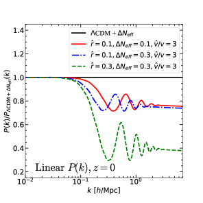
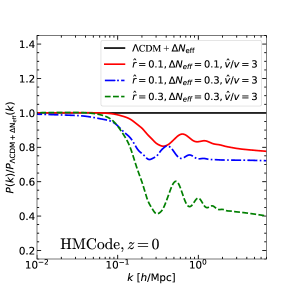
Figure 1: The linear (left panel) and non-linear (right panel) twin Higgs matter power spectrum for various twin parameters at $z=0$. Their cosmological parameters used for calculation are $h=0.676$, $\Omega_{b}h^{2}=0.0228$, $\Omega_{\rm cdm}h^{2}=0.121$, $\rm{ln}(10^{10}A_{s})=3.05$, $n_{s}=0.976$, and $\tau_{\rm reio}=0.061$.

The CMB and matter power spectra in MTH cosmology differ from those in the $\Lambda$CDM because of the presence of twin radiation and BAO Bansal:2021dfh . For the CMB TT and EE power spectra, the twin BAO suppresses the metric perturbations and enhances (decreases) the expansion (contraction) mode of temperature perturbations. In addition, scattering DR from the twin photon also changes the amount of phase shift for the oscillation peaks in the TT and EE spectra compared to the free-streaming DR scenarios. Both effects leave visible signals in the Planck measurement.

For the matter power spectrum, the presence of twin BAO suppresses the matter density perturbations at a small scale. Moreover, it introduces an oscillation in the power spectrum in addition to the SM BAO. In the left panel of Fig. 1, we present three benchmark linear matter power spectra with the same cosmological inputs $h=0.676$, $\Omega_{b}h^{2}=0.0228$, $\Omega_{\rm cdm}h^{2}=0.121$, $\rm{ln}(10^{10}A_{s})=3.05$, $n_{s}=0.976$, $\tau_{\rm reio}=0.061$. At small scale, $k\gtrsim 0.1~{}h\rm{Mpc}^{-1}$ that enters the horizon before the twin recombination epoch, the linear matter power spectrum deviates from that of $\Lambda\rm{CDM}+\Delta N_{\rm eff}$ with an oscillation and a suppression. Thus, the matter power spectrum in the scale $k\gtrsim 0.1~{}h\rm{Mpc}^{-1}$ is one of the best regions to test the MTH model. Coincidentally, this scale structure is testable by using weak lensing observations. In this work, we probe the matter distribution in this scale based on the DES cosmic shear data.

The linear evolution of density perturbations assumes the fractional density fluctuations $\delta(\rm{k})\ll 1$ so that correction from $\mathcal{O}(\delta(\rm k)^{2})$ terms is negligible. However, in the late universe, $\delta(\rm{k})$ can be comparable to or even greater than unity at $k=\mathcal{O}(0.1)~{}h{\rm Mpc}^{-1}$ and above, and the linear calculation no longer applies. Therefore, like computation performed in IDM-DR model Schaeffer_2021 ; Munoz:2020mue , we should, in principle, run $N$-body simulations to incorporate the non-linear corrections to the matter power spectrum up to $k\approx 10~{}h{\rm Mpc}^{-1}$ for the weak lensing analysis. However, the $N$-body simulation is much more CPU-time expansive, and having an event-by-event non-linear correction from the $N$-body simulation is unrealistic for the MCMC study.

In this work, we take the following approach to estimate the non-linear correction. First, as discussed later in Sec. 6, we run $N$-body simulations for two benchmarks MTH models and show that the resulting $P(k)$ correction is similar to the one obtained from the non-linear correction code, HMCode Mead_2016 . We then use the HMCode in the MCMC study for the non-linear correction at different redshift. In the right panel of Fig. 1, we show the power spectrum with non-linear correction computed by HMCode code. Compared with the linear power spectrum (the left panel), the non-linear effects smear the twin BAO structure at $z=0$, as discussed in Schaeffer_2021 for a more general setup of DAO models.

3 Cosmic shear

In this section, we describe the calculation of the two-point correlation function of the cosmic shear from the observational data and explain how we obtain the covariance matrix that models the uncertainties of the shear measurement. We also show an example of the shear spectrum for the MTH cosmology.

3.1 Cosmic shear measurement

The DES Y3 data measures the shapes of over $10^{8}$ source galaxies covering a footprint ${\rm A_{eff}}=4143~{}\rm{deg}^{2}$. Following the DES Y3 analysis, the shape catalog METACALIBRATION is divided by 4 redshift tomographic bins in the range of $0<z<3$ DES:2021bvc . In this work, we calculate the two-point correlation function of cosmic shear in the same manner.

Given a pair of galaxy images with angular separation $\theta$ in any two redshift bins ($i$ and $j$), we can express the shear-shear correlation function in terms of ellipticities that include the tangential component $\epsilon_{t}$ and the cross component $\epsilon_{\times}$,

$$\xi_{\pm}^{ij}(\theta)=\langle\epsilon^{i}_{t}\epsilon^{j}_{t}\rangle\pm\langle\epsilon^{i}_{\times}\epsilon^{j}_{\times}\rangle\,.$$ (1)

Here the brackets represent the average of all galaxies pairs. From the experimental observations, we can calculate the correlation function by summing all galaxy pairs (in the $i$ and $j$ redshifts) with indices $a$ and $b$ DES:2021vln ; DES:2017qwj ,

$$\xi_{\pm}^{ij}(\theta)=\frac{\sum_{ab}w_{a}w_{b}\left(\hat{e}_{t,a}^{i}\hat{e}_{t,b}^{j}\pm\hat{e}_{\times,a}^{i}\hat{e}_{\times,b}^{j}\right)}{\sum_{ab}w_{a}w_{b}R_{a}R_{b}},$$ (2)

where $w_{a}$ and $w_{b}$ are the weight of each galaxy pairs in $i$ and $j$ redshift bin, respectively. Notice that we modify the ellipticity expression in Eq. (2) by subtracting the residual mean shear, $\hat{e}_{k}^{i}=\epsilon_{k}^{i}-\langle\epsilon_{k}\rangle^{i}$. The response correction matrix $R$ comes from the linear order expansion of the ellipticities from a noisy and biased measurement ($\hat{e}$) with respect to the gravitational shear ($\xi_{\pm}$) that we want to extract DES:2020ekd . $R$ includes the measured shear response matrix $R_{\gamma}$ and the shear selection bias matrix $R_{S}$. We can explicitly write down the response correction as $R_{[k,l]}=R^{[k,l]}_{\gamma}+R^{[k,l]}_{S}$ for the $[k,l]$ element of the matrices, where $k,l=1,2$ that corresponds to the two shear degrees of freedom $t$ and $\times$. Following the analysis in Ref. DES:2017qwj , we take an average of each shear components $R_{a(b)}=(R_{[1,1]}+R_{[2,2]})/2$ for a galaxy $a(b)$ when calculating Eq. (2). We take the ellipticities $\hat{e}_{k}^{i}$ and the response correction matrix $R=R_{\gamma}+R_{S}$ from shape catalog METACALIBRATION. The cosmic shear data vector $\xi_{\pm}^{ij}$ can be obtained by using public code TreeCorr Jarvis:2003wq . All the auto correlations and cross correlations of the four redshift bins are calculated using 20 $\theta$-bins arranging logarithmically from $2.5$ to $250$ arcmin.

3.2 Covariance matrix

We model the statistical uncertainties of the $\xi_{\pm}$ measurement by hiring a covariance matrix $\mathbf{C}$ which can be calculated with public code CosmoCov Fang:2020vhc ; Krause:2016jvl . Note that the matrix $\mathbf{C}$ strongly depends on the per-component shape dispersion $\sigma_{e}$, galaxies’ redshift distribution (galaxy number densities), and cosmological parameters. Therefore, we should embed an unfixed $\mathbf{C}$ when performing a cosmological MCMC scan. However, such a scan is numerically challenging, and we instead take an approximation following the same analyses in the cosmic shear literature DES:2021bvc . First, we directly take the per-component shape dispersion $\sigma_{e}$ and galaxies effective number densities $n_{\rm eff}$ used in the covariance matrix from Table I of Ref. DES:2021bvc in the analysis. In order to shorten the scanning time, we use a set of fiducial parameters for the initial MCMC chains, namely {$\Omega_{m}=0.3$, $\Omega_{\Lambda}=0.7$, $\sigma_{8}=0.82355$, $n_{s}=0.97$, $\Omega_{b}=0.048$, $h=0.69$}. After the initial scans converge, we recompute the covariance matrix by using the best-fit parameters {$\Omega_{m}=0.306$, $\Omega_{\Lambda}=0.694$, $\sigma_{8}=0.802$, $n_{s}=0.974$, $\Omega_{b}=0.022$, $h=0.686$} and fix them for the later scans.

3.3 DM model prediction

The MTH theoretical prediction of the cosmic shear for two redshift bins ($i$ and $j$) is expressed as

$$\xi^{ij}_{\pm}(\theta)=\frac{1}{2\pi}{\int_{0}^{\infty}C_{\rm tot}^{ij}(\ell)J_{0/4}(\ell\cdot\theta)\ell d\ell},$$ (3)

where $\ell$ is the angular wave number. The Bessel function is the zeroth-order $J_{0}$ for $\xi_{+}$, but fourth-order $J_{4}$ for $\xi_{-}$. Under Limber approximation Limber:1953 ; LoVerde:2008re , we can derive the 2D shear-shear power spectrum $C_{GG}^{ij}(\ell)$ between redshift bin $i$ and $j$ in terms of the 3D matter power spectrum $P_{\delta}$,

$$C_{GG}^{ij}(\ell)=\int_{0}^{\chi_{\rm z_{max}}}d\chi\frac{W^{i}(\chi)W^{j}(\chi)}{\chi^{2}}P_{\delta}\left(k=\frac{\ell+1/2}{\chi},z(\chi)\right),$$ (4)

where $\chi$ is the comoving distance. We shall also consider contribution from the intrinsic alignment (IA) given in Appendix A, thus the total 2D spectrum is $C_{\rm tot}^{ij}(\ell)=C_{GG}^{ij}(\ell)+C_{GI}^{ij}(\ell)+C_{II}^{ij}(\ell)$. To save computation time, we only calculate the non-linear power spectrum ${\rm P_{\delta}}$ up to $k=10~{}h\rm{Mpc}^{-1}$ with the HMCode in CLASS. The lensing efficiency kernel $W^{i}(\chi)$ in the redshift bin $i$ is given by

$$W^{i}(\chi)=\frac{3H_{0}^{2}\Omega_{\mathrm{m}}}{2c^{2}}\frac{\chi}{a(\chi)}\int_{\chi}^{\chi_{\rm z_{max}}}d\chi^{\prime}n^{i}\left(\chi^{\prime}\right)\frac{\chi^{\prime}-\chi}{\chi^{\prime}},$$ (5)

where $n^{i}(z)$ is the normalized galaxies redshift distribution in the $i$-th redshift bin, and we have $\int n(\chi)d\chi=\int n(z)dz=1$. The scale factor is $a(\chi)$, and $c$ is the speed of light. It needs to note that in our analysis we have neglected the multiplicative bias and photometric redshift calibration uncertainties since both of them only affect the final results with a tiny deviation $\sim O(0.001)$ DES:2021bvc .

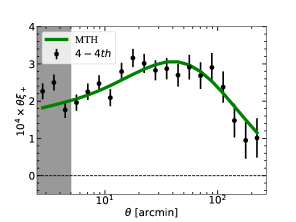
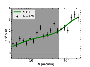
Figure 2: The auto two-point correlation function of cosmic shear for 4-4$th$ redshift bin. The data points correspond to DES Y3 cosmic shear measurement. The diagonal term of the covariance matrix gives the error bars of data points. The green solid lines are computed by HMCode. The gray region is masked to avoid the small-scale uncertainties as applied in Ref. DES:2021bvc .

In Fig. 2, we demonstrate $\xi^{44}_{+}$ (left panel) and $\xi^{44}_{-}$ (right panel) as an example, because the 4-4$th$ redshift bin presents the most foreground lensing effect. For the results of the rest redshift bins, we refer them to Fig. 10 in Appendix. B. Here, the black data points present the DES Y3 cosmic shear measurement, and the error bars denote the diagonal term of the covariance matrix. To reduce the impact of non-linear baryonic effects, we exclude data below certain $\theta$ (gray) as recommended in Ref. DES:2021bvc , which is based on hydrodynamic simulations. As a comparison, we compute the best-fit MTH prediction (green solid line) based on the parameter configuration: {$\Omega_{b}h^{2}=0.023$, $\Omega_{\rm cdm}h^{2}=0.121$, $\theta_{s}=1.042$, $\rm{ln}(10^{10}A_{s})=3.034$, $n_{s}=0.975$, $\tau_{\rm reio}=0.051$, $\hat{r}=0.067$, $\hat{v}/v=2.725$, $\Delta\hat{N}=0.168$}.

4 Methodology

In this section, we briefly discuss the likelihoods and priors used in the MCMC scan of the MTH and cosmological parameter space. We employ Bayes’s theorem to find the posterior probability density function,

$${\rm Posterior}\propto{\rm Likelihood}\times{\rm Prior}.$$ (6)

The normalization of the posterior called “evidence” is a quantity relevant to the model comparison. Our results are presented by marginalizing the posterior densities of unwanted parameters and showing the $68\%$ and $95\%$ credible regions.

Parameter	Prior distribution	Prior range
Cosmology
$\Omega_{b}h^{2}$	Flat	[0.022, 0.023]
$\Omega_{\rm cdm}h^{2}$	Flat	[0.112, 0.128]
$100\cdot\theta_{s}$	Flat	[1.039, 1.043]
$\ln\left(A_{s}\times 10^{10}\right)$	Flat	[2.955, 3.135]
$n_{s}$	Flat	[0.941, 0.991]
$\tau_{\rm reio}$	Flat	[$10^{-2}$, 0.7]
Mirror twin Higgs
$\hat{r}$	Flat	[$10^{-3}$, 1]
$\hat{v}/v$	Flat	[2, 15]
$\Delta\hat{N}$	Flat	[$10^{-3}$, 1]
Intrinsic alignment
$A_{\rm IA}$	Flat	[-6, 6]
$\eta$	Flat	[-6, 6]

Table 1: All the input parameters used in our scan. Three types of parameters are grouped as cosmological, MTH, and intrinsic alignment parameters.

To explore the MTH model parameter space, we conduct a global scan by using a public cosmological MCMC package Monte Python Brinckmann:2018cvx ; Audren:2012wb , and it interfaces with CLASS to compute the cosmological observables. In Table 1, we show the prior ranges used in our numerical scan, including $\Lambda$CDM parameters as defined in planck and MTH parameters: the fraction of the twin baryon to DM energy density $\hat{r}$, the ratio of vacuum expectation value between the twin and SM sectors $\hat{v}/v$, and the extra effective number of neutrinos from the twin sector $\Delta\hat{N}$.

We apply five likelihood sets in the MCMC study. For setting existing bounds on the MTH model, we consider three datasets

1. The cosmic shear likelihood based on the DES Y3 METACALIBRATION shape catalog, which described in Sec. 3.

2. The CMB likelihoods are calculated based on Planck 2018 Legacy Planck:2019nip , including high-$\ell$ power spectra (TT, TE, and EE), low-$\ell$ power spectrum (TT and EE), and Planck lensing power spectrum (lensing).

3. The BAO likelihood contains the BOSS DR12 dataset measurements at $z=0.106$, $z=0.15$ and $z=0.2-0.75$  Beutler_2011 ; Ross_2015 ; Alam_2017 .

When studying how MTH can relax the $H_{0}$ and $S_{8}$ tensions, we further include two datasets one by one

1. The SH0ES likelihood is also a Gaussian distribution with the measurement Riess:2021jrx

   $$H_{0}=73.04\pm 1.04\mathrm{~{}km}\mathrm{~{}s}^{-1}\mathrm{Mpc}^{-1}.$$

2. The Planck SZ (2013) likelihood is described by a Gaussian distribution with the measurement Ade:2013lmv

   $$S_{8}^{\mathrm{SZ}}\equiv\sigma_{8}\left(\Omega_{\mathrm{m}}/0.27\right)^{0.3}=0.782\pm 0.010.$$

We would like to note that $S_{8}^{\mathrm{SZ}}$ here differs from the definition of $S_{8}$ used in this work. The $S_{8}^{\rm SZ}$ value is in $2-3\sigma$ tension to the $\Lambda$CDM fit of the CMB data. However, as mentioned in the introduction, the measurements of galaxy distribution from the SZ effect depend on a mass bias factor $(1-b)$ that relates the observed SZ signal to the true mass of galaxy clusters. The Planck SZ (2013) report gives an $S_{8}$ measurement by fixing the mass bias to its central value from a numerical simulation, $(1-b)=0.8$. The Planck SZ (2015) report later allowed $(1-b)$ to vary with a Gaussian prior centered at $0.79$. The central value of the resulting $S^{\rm SZ}_{8}$ becomes smaller but has a much larger uncertainty $S_{8}^{\rm SZ}=0.744\pm 0.034$ Planck:2015lwi and less tension to CMB measurements. Nevertheless, since the central value of the $\sigma_{8}$ from the SZ (2013) analysis ($\sigma_{8}=0.76$ for $\Omega_{m}=0.3$) is consistent with most of the low-redshift measurements 2022JHEAp..34…49A , future LSS measurements may converge to the SZ (2013) result with a better-determined bias factor. Therefore, including the SH0ES and the SZ (2013) datasets help demonstrate the MTH model’s capability to simultaneously solve the $H_{0}$ and $S_{8}$ problems when both tensions increase to $3-4\sigma$ in the future.

In the MCMC study, we implement all the likelihood from the Monte Python except for the DES cosmic shear. We implement the cosmic shear likelihood function as

$$\ln\mathcal{L}_{\rm shear}=-\frac{1}{2}\sum_{ij}\left(D_{i}-T_{i}\right)\left[\mathbf{C}^{-1}\right]_{ij}\left(D_{j}-T_{j}\right),$$ (7)

where $T$ and $D$ are the theoretically predicted and experimentally measured shear-shear correlation functions, respectively. We obtain the covariance matrix $\mathbf{C}$ from a procedure described in Sec. 3.2. Note that we mask the small scale data to avoid the small scale uncertainties as applied in Ref. DES:2021bvc , because the baryon feedback effect at small scale (e.g. AGN feedback or star-forming feedback) remains largely unknown.

We perform four MCMC scans step-by-step for the MTH model based on the likelihoods stated in the section: Planck+BAO, Planck+BAO+DES Y3, Planck+BAO+DES Y3+SH0ES and Planck+BAO+DES Y3+SZ (2013)+SH0ES. As a comparison, four scans for $\Lambda$CDM based on the same likelihoods are also performed. In each scan, we collect 8 chains with approximately 0.5 million samples in total. The average acceptance rate is around $0.2$.

5 Results

This section presents the MTH parameter space favored by four different combinations of datasets described in Sec. 4: (i) by fitting the Planck+BAO and Planck+BAO+DES Y3 data, we show the current credible region of the MTH parameters. (ii) by fitting the Planck+BAO+DES Y3+SH0ES data, we show that the MTH model can accommodate a larger $H_{0}$ and smaller $S_{8}$ compared to the $\Lambda$CDM and $\Lambda$CDM+$\Delta N_{\rm eff}$ models. (iii) to further examine MTH model’s ability to resolve the $S_{8}$ tension, we compare the MTH and $\Lambda$CDM models based on the likelihood Planck+BAO+DES Y3+SH0ES+SZ (2013). (iv) finally, to show the prospect of measuring the MTH parameters with the future CSST, we generate mock data using a benchmark MTH model and perform a fit to the Planck+BAO+SH0ES+SZ (2013)+CSST likelihood.

5.1 CMB, BAO and Weak Lensing

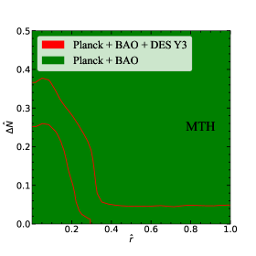
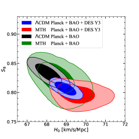
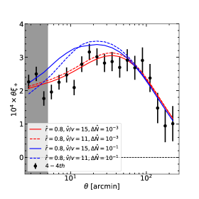
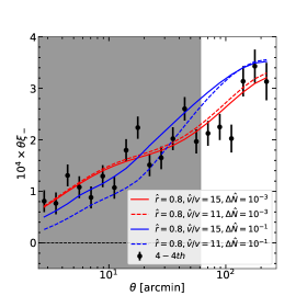
Figure 3: The two dimensional posterior distributions for MTH parameters $\hat{r}$ and $\Delta\hat{N}$ (upper left panel) as well as cosmological parameters $H_{0}$ and $S_{8}$ (upper right panel). The contours show the 68% (inner contour) and 95% (outer contour) credible regions. The green contours are based on the likelihood of Planck+BAO, while the likelihood for the red contours additionally includes the DES Y3 cosmic shear data. Here we use the HMCode for the non-linear correction as discussed in Sec. 2 and 6. The black (blue) contours are based on the likelihood of Planck+BAO (Planck+BAO+DES Y3) for the $\Lambda$CDM model. The two bottom graphs show the auto two-point correlation function of cosmic shear in 4-4th redshift bin for $\xi_{+}$ (bottom left panel) and $\xi_{-}$ (bottom right panel). The red lines denote the MTH parameters $\hat{r}=0.8$, $\Delta\hat{N}=0.001$ with $\hat{v}/v=15$ (solid line) and $\hat{v}/v=11$ (dashed line). The blue lines denote the MTH parameters $\hat{r}=0.8$, $\Delta\hat{N}=0.1$ with $\hat{v}/v=15$ (solid line) and $\hat{v}/v=11$ (dashed line).

Parameters	$\Lambda\mathrm{CDM}$		MTH
	best-fit	$\operatorname{mean}\pm\sigma$	best-fit	$\operatorname{mean}\pm\sigma$
$100\Omega_{b}h^{2}$	2.262	$2.256_{-0.0131}^{+0.0132}$	2.262	$2.263_{-0.015}^{+0.014}$
$\Omega_{\rm cdm}h^{2}$	0.1179	$0.1177_{-0.00071}^{+0.00074}$	0.1192	$0.1196_{-0.0023}^{+0.0014}$
$100\theta_{s}$	1.042	$1.042_{-0.00028}^{+0.0003}$	1.042	$1.042_{-0.00033}^{+0.00035}$
$\ln\left(10^{10}A_{s}\right)$	3.023	$3.034_{-0.014}^{+0.014}$	3.049	$3.038_{-0.015}^{+0.015}$
$n_{s}$	0.9713	$0.9709_{-0.00349}^{+0.00353}$	0.9701	$0.9729_{-0.0047}^{+0.0039}$
$\tau_{\text{reio }}$	0.04851	$0.05194_{-0.0071}^{+0.0071}$	0.05741	$0.05231_{-0.0073}^{+0.0074}$
$\hat{r}$	–	–	0.0375	$0.1812_{-0.1802}^{+0.015}$
$\hat{v}/v$	–	–	2.3625	$7.707_{-5.707}^{+2.051}$
$\Delta\hat{N}$	–	–	0.0435	$0.1064_{-0.1054}^{+0.0319}$
$\Omega_{m}$	0.2954	$0.295_{-0.0043}^{+0.0041}$	0.2973	$0.294_{-0.0051}^{+0.0049}$
$H_{0}$	68.97	$68.97_{-0.349}^{+0.344}$	69.06	$69.55_{-0.76}^{+0.49}$
$S_{8}$	0.8038	$0.8067_{-0.0073}^{+0.0075}$	0.802	$0.797_{-0.0093}^{+0.012}$
$-2\ln\mathcal{L}$	3032.4		3031.74
Planck + BAO	2791.28		2789.06
DES Y3	241.12		242.68

Table 2: The mean and best-fit values for the $\Lambda$CDM and MTH models obtained including the Planck+BAO+DES Y3 likelihoods.

We start with a comparison between two scans; one uses the likelihood only containing the Planck and BAO data (Planck+BAO), and the other one further includes the DES Y3 cosmic shear likelihood (Planck+BAO+DES Y3). In the top left panel of Fig. 3, we present the 68% (inner contour) and 95% (outer contour) credible regions projected on the ($\hat{r}$, $\Delta\hat{N}$) plane. The likelihoods of green contours are Planck+BAO, while the red contours are based on the Planck+BAO+DES Y3 likelihood.

We can clearly see two interesting features in the plot by comparing the allowed region between Planck+BAO and Planck+BAO+DES Y3. First, for $\Delta\hat{N}>0.06$, $\hat{r}$ has an upper limit $\hat{r}\lesssim 0.3$ for the $95\%$ credible region from the inclusion of the DES likelihood. The bound gets much stronger than the result in Bansal:2021dfh (Fig. 21) with only the Planck+BAO data. The upper bound on $\hat{r}$ owes to the effect that the matter power spectrum predicted by the MTH model is suppressed due to the twin BAO (Fig. 1). The suppression increases with $\hat{r}$ for a given $(\Delta\hat{N},\hat{v}/v)$, and if $\hat{r}$ becomes too large, the model can no longer fit the DES data well. Our prior has an upper bound $\hat{v}/v\leq 15$, which corresponds to a better than $\approx 1\%$ tuning of the model Craig:2015pha . For $\Delta\hat{N}>0.06$, even if $\hat{v}/v\approx 15$, the twin recombination still occurs late enough so that the DES data is sensitive to the power spectrum suppression. Conversely, a smaller value of $\Delta\hat{N}$ corresponds to colder MTH particles and an earlier twin recombination process, resulting in the twin baryon behaving like CDM at an earlier time. At the bottom of Fig.3, it is shown that we can improve the fit of the cosmic shear data by decreasing $\Delta\hat{N}$ from 0.1 (blue line) to 0.001 (red line) for large $\hat{r}=0.8$. However, increasing the value of $\hat{v}/v$ does not significantly improve the fit, particularly within our prior range of $\hat{v}/v\leqslant 15$. Therefore, to relax the constraint on $\hat{r}$, a colder mirror sector is needed, which is reflected by a smaller value of $\Delta\hat{N}$ (as is also illustrated in Fig. 11). Another interesting feature in the plot is that when $\hat{r}<0.2$, the upper bounds on $\Delta\hat{N}$ from the red curves extend to higher values than the green curves. The weaker $\Delta\hat{N}$ bound indicates that the DES Y3 data prefer a slightly warmer mirror sector that can result in more significant suppression of the matter power spectrum. Moreover, as discussed in Ref. Bansal:2021dfh , the presence of twin photons as scattering radiation (before the twin recombination) also weakens the $\Delta N_{\rm eff}$ constraints in the MTH model compared to the free-streaming radiation.

In the upper right panel of Fig. 3, we present the preferred region of $(H_{0},S_{8})$ from fitting the MTH (green and red) and $\Lambda$CDM (black and blue) models. Compared to the fit without the DES Y3 data, both the $\Lambda$CDM and MTH contours move to smaller $S_{8}$ regions, indicating that the DES Y3 data prefers a smaller matter power spectrum in the scale $0.1\lesssim k\lesssim 10\,h$Mpc^-1 than the model predictions from fitting the CMB and BAO data. In the MTH model, the mirror radiation and the twin acoustic oscillation process can enhance $H_{0}$ while keeping a small $S_{8}$, providing a chance to relax both tensions. Notice that the MTH model has a limit to the $\Lambda$CDM model either with $\hat{r}\to 0$ or $\Delta\hat{N}\to 0$. This means that the MTH contours contain the best-fit points of the $\Lambda$CDM model, and the larger MTH contours do mean that the model can accommodate a larger $H_{0}$ and a smaller $S_{8}$ compared to the $\Lambda$CDM. The red contour in the plot has $H_{0}=69.56_{-0.76}^{+0.49}$ km s^-1Mpc^-1, and the Gaussian Tension to the SH0ES result is $2.8\sigma$ compared to the $\Lambda$CDM result $H_{0}=69.0_{-0.35}^{+0.34}$ km s^-1Mpc^-1 and $3.7\sigma$. Although the Gaussian Tension is only a rough measure of disagreement between measurements, the numbers indeed show an improvement in relaxing the $H_{0}$ tension.

5.2 Likelihoods including SH0ES

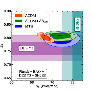
Figure 4: Marginalized 2D posterior distribution in the ($H_{0}$ , $S_{8}$) plane with Planck+BAO+DES Y3+SH0ES. The orange contour corresponds to the $\Lambda\rm{CDM}$ model, the green contour corresponds to the $\Lambda\rm{CDM}+\Delta N_{\rm eff}$ model and the blue contour corresponds to the MTH model. The dark cyan band corresponds to the $1\sigma$ (inner) and $2\sigma$ (outer) region of the SH0ES result Riess:2021jrx , and the purple band corresponds to the $S_{8}$ obtained by a blind analysis in the context of the $\Lambda$CDM model DES:2021bvc .

Parameters	$\Lambda\mathrm{CDM}$		$\Lambda\mathrm{CDM}+\Delta N_{\rm eff}$		MTH
	best-fit	$\operatorname{mean}\pm\sigma$	best-fit	$\operatorname{mean}\pm\sigma$	best-fit	$\operatorname{mean}\pm\sigma$
$100\Omega_{b}h^{2}$	2.270	$2.268_{-0.0148}^{+0.0099}$	2.275	$2.282_{-0.0175}^{+0.0115}$	2.273	$2.283_{-0.017}^{+0.012}$
$\Omega_{\rm cdm}h^{2}$	0.1166	$0.1167_{-0.0005}^{+0.0009}$	0.1204	$0.1211_{-0.0026}^{+0.017}$	0.1210	$0.1224_{-0.0028}^{+0.0021}$
$100\theta_{s}$	1.042	$1.042_{-0.0003}^{+0.0002}$	1.042	$1.042_{-0.00032}^{+0.00046}$	1.042	$1.042_{-0.00035}^{+0.00042}$
$\ln\left(10^{10}A_{s}\right)$	3.048	$3.044_{-0.016}^{+0.012}$	3.052	$3.05_{-0.016}^{+0.012}$	3.054	$3.051_{-0.016}^{+0.013}$
$n_{s}$	0.9735	$0.9736_{-0.0041}^{+0.0028}$	0.9803	$0.9811_{-0.0062}^{+0.0038}$	0.9740	$0.9795_{-0.0054}^{+0.0036}$
$\tau_{\text{reio }}$	0.0595	$0.0572_{-0.0082}^{+0.0060}$	0.05784	$0.0555_{-0.0074}^{+0.0067}$	0.05866	$0.05566_{-0.0074}^{+0.0068}$
$\hat{r}$	–	–	–	–	0.1144	$0.1128_{-0.076}^{+0.091}$
$\hat{v}/v$	–	–	–	–	9.62	$8.98_{-4.04}^{+3.76}$
$\Delta\hat{N}$	–	–	0.2071	$0.2588_{-0.1545}^{+0.093}$	0.1979	$0.3098_{-0.1520}^{+0.0950}$
$\Omega_{m}$	0.2908	$0.2901_{-0.0040}^{+0.0039}$	0.288	$0.2873_{-0.0041}^{+0.0041}$	0.2915	$0.2895_{-0.005}^{+0.0046}$
$H_{0}$	69.51	$69.48_{-0.43}^{+0.21}$	70.5	$70.65_{-0.732}^{+0.775}$	70.22	$71.04_{-0.92}^{+0.52}$
$S_{8}$	0.8159	$0.8145_{-0.0055}^{+0.0052}$	0.8086	$0.8062_{-0.0078}^{+0.0078}$	0.8034	$0.794_{-0.0099}^{+0.0117}$
$-2\ln\mathcal{L}$	3046.49		3042.76		3042.21
Planck+BAO	2794.87		2794.27		2792.9
DES Y3	240.09		242.52		241.81
SH0ES	11.53		5.966		7.355

Table 3: The mean and best-fit values for the $\Lambda$CDM, $\Lambda$CDM+$\Delta N_{\rm eff}$, and MTH models obtained including the Planck+BAO+DES Y3+SH0ES likelihoods.

In order to test whether the MTH model could alleviate $H_{0}$ tension and $S_{8}$ tensions compared to the $\Lambda$CDM, we have included the SH0ES data in our fitting. In Fig. 4, we show the ($H_{0},S_{8}$) results based on three different models: $\Lambda$CDM, $\Lambda\rm{CDM}+\Delta N_{\rm{eff}}$ and MTH. For comparison, we show the $1$ and $2\sigma$ preferred region of the $S_{8}$ obtained by a blind analysis in the context of the $\Lambda$CDM model  DES:2021bvc (purple band). We also show the $1$ and $2\sigma$ preferred regions from the SH0ES measurement Riess:2021jrx (dark cyan band). The $\Lambda$CDM model is in significant tension to both measurements, especially the SH0ES. When using the $\Lambda$CDM+$\Delta N_{\rm{eff}}$ model to reduce the $H_{0}$ tension, the tension in $S_{8}$ gets a bit worse than the $\Lambda$CDM result. On the other hand, the MTH contour can extend to a larger $H_{0}$ while having a smaller $S_{8}$ value. This indicates that the MTH model has the potential to alleviate both $H_{0}$ and $S_{8}$ tensions, rather than worsening the $S_{8}$ tension as the $\Lambda\rm{CDM}+\Delta N_{\rm{eff}}$ model. However, since the $S_{8}$ tension in the DES Y3 data is not as significant as the SH0ES $H_{0}$ tension, the likelihood ratio $-2\ln(\mathcal{L}_{\rm MTH}/\mathcal{L}_{\Lambda\rm{CDM}})=-4.28$ is only slightly lower than $-2\ln(\mathcal{L}_{\Lambda\rm{CDM}+\Delta N_{\rm{eff}}}/\mathcal{L}_{\Lambda\rm{CDM}})=-3.73$. Given that the MTH model has three more parameters than $\Lambda$CDM, the model does not perform better than the $\Lambda\rm{CDM}+\Delta N_{\rm{eff}}$ model in fitting the Planck+BAO+DES Y3+SH0ES data.

Suppose the future $S_{8}$ measurements converge to the mean value of the DES Y3 result (center of the purple band in Fig. 4), but with the error drops by a factor of two. In that case, the $S_{8}$ will be close to the Planck SZ (2013) result, and the significance of the $S_{8}$ tension will be comparable to the current $H_{0}$ problem. Based on the scenario, we will show that the MTH model can provide a much better fit to the data if the $S_{8}$ tension worsens.

5.3 Likelihoods including Planck SZ (2013)

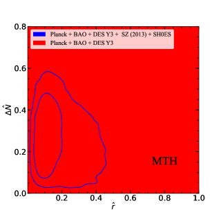
Figure 5: Marginalized posterior distribution similar to Fig. 3 but for a comparison between Planck+BAO+DES Y3 (red contours) and Planck+BAO+DES Y3+SZ (2013)+SH0ES (blue contours).

In Fig. 5, we compare the credible regions of Planck+BAO+DES Y3 (red contours) and Planck+ BAO+DES Y3+SZ (2013)+SH0ES (blue contours) for the MTH. The worse $S_{8}$ tension in the Planck SZ (2013) data than in the DES Y3 pushes the upper bound on $\hat{r}$ to a higher value. Moreover, both the $\hat{r}$ and $\Delta\hat{N}$ in this case have non-zero lower limits of the $95\%$ credible region, namely $0.02\lesssim\hat{r}\lesssim 0.4$ and $0.03\lesssim\Delta\hat{N}\lesssim 0.5$. Hence, the SZ (2013)+SH0ES likelihood prefers a non-vanishing twin matter component with a high enough temperature to sustain the twin BAO process. On the other hand, the suppression of the matter power spectrum cannot be too significant to violate the cosmic shear constraints. Hence, the dataset favors a particular range of non-zero $\hat{r}$. Similar results have also been shown in Ref. Bansal:2021dfh . However, we find the upper limits for $\hat{r}$ as shown in Fig. 5 for the first time. In Fig. 6, we show a comparison between the $\Lambda$CDM (orange contour) and MTH (blue contour) based on the likelihood scenario Planck+BAO+DES Y3+SZ (2013)+SH0ES. Although the MTH model has a continuous limit ($\hat{r}\to 0$ and $\Delta\hat{N}\to 0$) to reproduce the fit of $\Lambda$CDM model, the dataset pushes the MTH contour to a much lower $S_{8}$ and larger $H_{0}$ region. Although $\Lambda$CDM+$\Delta N_{\rm eff}$ model can also accommodate a larger $H_{0}$, it does a worse job in resolving the $S_{8}$ tension. Compared to the +$\Delta N_{\rm eff}$ model, the MTH can further reach the region that resolves both tensions.

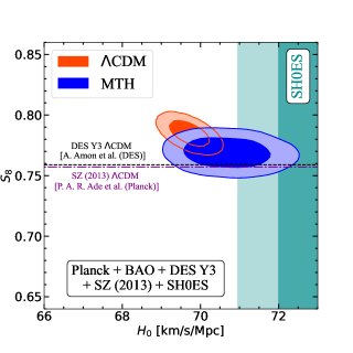
Figure 6: Marginalized posterior distribution of the scanning scenario Planck+BAO+DES Y3+SZ (2013)+SH0ES for $\Lambda$CDM (orange contour) and MTH (blue contour). The dark cyan band corresponds to the $95\%$ region of $H_{0}$ measured by SH0ES collaboration. Two dashed lines denote the central value of $S_{8}$ from DES Y3 and Planck SZ (2013) measurement.

Param	$\Lambda\mathrm{CDM}$		MTH
	best-fit	$\operatorname{mean}\pm\sigma$	best-fit	$\operatorname{mean}\pm\sigma$
$100\Omega_{b}h^{2}$	2.272	$2.273_{-0.015}^{+0.011}$	2.286	$2.285_{-0.018}^{+0.012}$
$\Omega_{\rm cdm}h^{2}$	0.1164	$0.1159_{-0.00052}^{+0.00089}$	0.1205	$0.1226_{-0.0028}^{+0.0020}$
$100\theta_{s}$	1.042	$1.042_{-0.00031}^{+0.00025}$	1.042	$1.042_{-0.00034}^{+0.00040}$
$\ln\left(10^{10}A_{s}\right)$	3.03	$3.026_{-0.016}^{+0.011}$	3.034	$3.046_{-0.016}^{+0.013}$
$n_{s}$	0.9749	$0.9744_{-0.0041}^{+0.0029}$	0.9747	$0.9772_{-0.0051}^{+0.0034}$
$\tau_{\text{reio }}$	0.05286	$0.05_{-0.0082}^{+0.0059}$	0.05058	$0.05419_{-0.0076}^{+0.0068}$
$\hat{r}$	–	–	0.06745	$0.1537_{-0.074}^{+0.087}$
$\hat{v}/v$	–	–	2.725	$5.968_{-2.513}^{+2.329}$
$\Delta\hat{N}$	–	–	0.1676	$0.3002_{-0.1449}^{+0.0898}$
$\Omega_{m}$	0.2867	$0.2856_{-0.0039}^{+0.0040}$	0.2908	$0.29_{-0.0050}^{+0.0051}$
$H_{0}$	69.65	$69.72_{-0.34}^{+0.33}$	70.23	$70.71_{-0.72}^{+0.70}$
$S_{8}$	0.7896	$0.7847_{-0.0065}^{+0.0065}$	0.7631	$0.769_{-0.0082}^{+0.0082}$
$-2\ln\mathcal{L}$	3063.72		3048.68
Planck + BAO	2798.51		2801.012
DES Y3	238.2		239.3
SZ (2013)	16.39		1.068
SH0ES	10.625		7.3

Table 4: The mean and best-fit values for the $\Lambda$CDM and MTH models obtained including the Planck+BAO+DES Y3+SH0ES+SZ (2013) likelihoods.

To further show that the MTH provides a much better fit to this dataset, we show the best-fit parameters and the associated likelihood $-2\mathcal{L}$ of the two models in Table. 4. The likelihood ratio $-2\ln(\mathcal{L}_{\rm MTH}/\mathcal{L}_{\Lambda\rm{CDM}})=-15.04$ implies that the MTH indeed fits the likelihoods better even if the model has three more parameters. Adding three extra degrees of freedom is also statistically unimportant because the total number of degrees of freedom is much larger. The likelihood improvement mainly comes from the better fit of the SH0ES and Planck SZ data. Compared with the MTH fit in Table. 2 without SH0ES+SZ (2013), we find that most of the best-fitted $\Lambda$CDM parameters change mildly. However, the MTH model parameters vary substantially between the two cases, which implies that the MTH sector is essential in alleviating two tensions.

5.4 Forecast of DM detection from the CSST sensitivity

If the tension in the $H_{0}$ value persists and the $S_{8}$ parameter converges to the Planck SZ (2013) result, as discussed in the previous section, the MTH model predicts non-zero values for the twin baryon and twin radiation energy densities when fit to cosmological data. This raises the interesting question of how precisely we can measure the abundance of twin particles with future experiments and surveys, assuming that the MTH model accurately describes the universe.

To address this question, we use the expected sensitivity of the upcoming CSST experiment to project the uncertainties in measuring the MTH parameters. Taking the same analysis procedure performed for DES Y3 in Sec. 3, we mock the future CSST likelihood by taking the central values of the data ($D$) in Eq. (7) to be the shear-shear correlation function calculated based on the MTH parameters {$\Omega_{b}h^{2}=0.02281$, $\Omega_{\rm cdm}h^{2}=0.1237$, $\theta_{s}=1.042$, $\rm{ln}(10^{10}A_{s})=3.037$, $n_{s}=0.9774$, $\tau_{\rm reio}=0.05094$, $\hat{r}=0.1047$, $\hat{v}/v=4.791$, $\Delta\hat{N}=0.3071$}. The numbers are within the $1\sigma$ region of the fit shown in Table. 4. When calculating Eq. (7), we adopt a relatively conservative per-component shape dispersion of the covariance matrix, $\sigma_{e}=0.3$ Gong:2019yxt . Using the redshift distributions in Ref. Lin:2022aro , we perform an MCMC scan by encoding the mock CSST data in Planck+BAO+CSST+SZ (2013)+SH0ES likelihood.

The results of the MTH model between two scenarios before and after updating the future CSST cosmic shear likelihood are presented in the left panel of Fig. 7. Attributing to a larger effective area and more galaxies to be observed in the CSST, the uncertainties of $\xi_{\pm}$ are significantly reduced at most a factor $\sim 10$. Hence, the most anticipated feature is the $95\%$ credible regions on the ($\hat{r}$, $\Delta\hat{N}$) plane (left panel) and ($H_{0}$ , $S_{8}$) plane (right panel) that significantly shrunk to the region near the central value, providing a $10\%$ ($1\%$) level precision measurement of $0.09<\hat{r}<0.12$ ($0.764<S_{8}<0.773$).

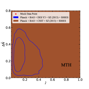
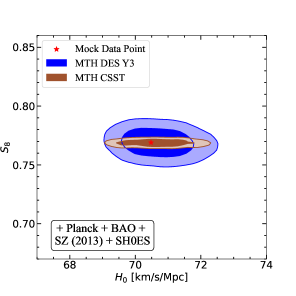
Figure 7: Marginalized 2D posterior distribution in the ($\hat{r}$ , $\Delta\hat{N}$) plane (left panel) and the the ($H_{0}$ , $S_{8}$) plane (right panel), assuming a mock data point (red star):{$\Omega_{b}h^{2}=0.02281$, $\Omega_{\rm cdm}h^{2}=0.1237$, $\theta_{s}=1.042$, $\rm{ln}(10^{10}A_{s})=3.037$, $n_{s}=0.9774$, $\tau_{\rm reio}=0.05094$, $\hat{r}=0.1047$, $\hat{v}/v=4.791$, $\Delta\hat{N}=0.3071$}. The brown contours are the MTH result of Planck+BAO+CSST+SZ (2013)+SH0ES in comparison to the Planck+BAO+DES Y3+SZ (2013)+SH0ES for the MTH (blue contours). Two dashed lines denote the central value of $S_{8}$ from DES Y3 and Planck SZ (2013) measurement.

6 Non-linear corrections: HMCode, Halofit vs. $N$-body simulation

In this section, we justify the use of HMCode in our MCMC analysis by comparing the non-linear power spectra of two benchmark MTH models computed using HMCode and the gravity only $N$-body simulation.

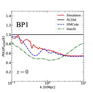
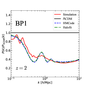
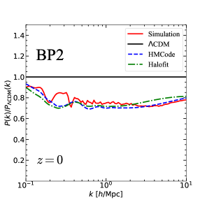
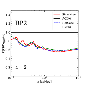
Figure 8: The ratio of matter power spectrum between MTH model and $\Lambda\rm{CDM}$. The numerical results are computed by the public nonlinear codes (Halofit and HMCode) and $N$-body simulation at $z=0$ (left panel) and $z=2$ (right panel) for BP1 (upper panel) and BP2 (lower panel). The red solid lines are the results obtained by the $N$-body simulation, while the green dashed-dotted lines and the blue dashed lines correspond to the results given by Halofit and HMCode, respectively.

We perform our $N$-body simulations with the code P-Gadget3, a TreePM code based on the publicly available code Gadget2 Springel:2005mi . We start our simulation from the redshift $z=127$ with the initial condition generated by the code 2LPTic Crocce:2006ve whose input power spectrum can be obtained by using CLASS. We use the matter power spectra generated by two different MTH models in the study. The two benchmark models, which we call BP1 and BP2, have the MTH parameters {$\hat{r}=0.25$, $\hat{v}/v=6.31$, $\Delta\hat{N}=0.35$} and {$\hat{r}=0.10$, $\hat{v}/v=3.00$, $\Delta\hat{N}=0.30$}, and the other cosmological parameters relevant to the power spectrum calculation are

• : {$\Omega_{\rm m}=0.2936$, $\Omega_{\Lambda}=0.7064$, $h=0.7084$, $n_{\rm s}=0.9727$, $\sigma_{8}=0.7599$},

• : {$\Omega_{\rm m}=0.3254$, $\Omega_{\Lambda}=0.6746$, $h=0.6756$, $n_{\rm s}=0.9727$, $\sigma_{8}=0.7648$}.

In the gravity-only simulation we perform, the code only takes the total matter density $\Omega_{\rm m}=\Omega_{\rm cdm}+\Omega_{b}$. Since Gadget only reads the input power spectrum shape, we calculate the $\sigma_{8}$ of each model separately and feed them to Gadget to calibrate the power spectrum. We run the $N$-body simulation with $N_{0}=512^{3}$ particles in a periodic box of volume $(200~{}{\rm Mpc}/h)^{3}$. The mass of a simulation particle is $4.733\times 10^{9}M_{\odot}/h$ in the simulations.

In Fig. 8, we show the ratio of matter power spectra between the MTH and $\Lambda\rm{CDM}$ models obtained using the $N$-body simulation (red solid line), Halofit (green dash-dotted line), and HMCode (blue dashed line). We use the Halofit for the non-linear correction to the $P_{\Lambda{\rm CDM}}$ since the code has been tuned to mimic the $N$-body results of the $\Lambda$CDM model. As we can see from the red curves, although some features of the twin acoustic oscillations remain visible from the $N$-body simulation at $z=2$ (right panel), the features get smoothed out at $z=0$ (left panel), similar to the findings in Ref. Schaeffer_2021 ; Munoz:2020mue . The minor kinks at $k<0.3~{}h/\rm{Mpc}$ come from statistical fluctuations.

For $k\geq 1\,h$Mpc^-1, HMCode generate power spectra that agree well with the $N$-body simulation results. For $0.3\lesssim k\lesssim 1\,h$Mpc^-1, the results deviate more due to the less severe damping of the oscillation pattern predicted by the HMCode. However, the difference to the $N$-body simulation is only up to $\approx 20\%$ for the BP1 with $k$-mode around $k=0.4\,h$Mpc^-1. The deviation is comparable to the fractional uncertainties $\approx 10\%$ in the DES Y3 data.

Given that the HMCode reproduces the general behavior of the $N$-body simulation results in these examples, and the oscillation patterns only remain in a small $k$ window and have amplitudes comparable to the experimental uncertainty, we believe the code can provide a reasonable estimate of the MTH spectrum for our MCMC study. Since the $N$-body simulation is much more time-consuming, using HMCode in the analysis is the best of what we can do now for the study. However, different from the HMCode, Halofit produces a much more different power spectrum in the BP1 case at $z=0$, and it is hard to explain the origin of the deviation. We therefore do not use Halofit in the MCMC study.

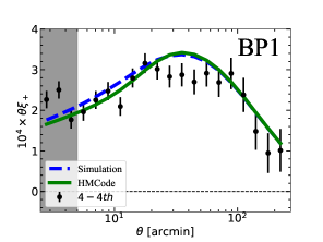
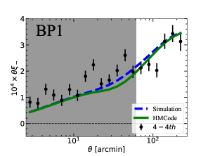
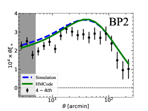
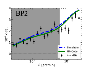
Figure 9: The cosmic shear of the 4-4${th}$ redshift bin obtained for the BP1 (upper) and BP2 (lower) models. The data points correspond to the DES Y3 cosmic shear measurement. The diagonal term of the covariance matrix gives the error bars of data points. The gray region is masked to avoid the small scale uncertainties as applied in Ref. DES:2021bvc . The blue dashed lines correspond to the calculation based on the $N$-body simulation correction, while the green solid lines correspond to the calculation based on the HMCode. The difference between the $N$-body simulation and HMCode calculation is within the size of the error bars and mainly shows up within the masked (gray) region.

To better quantify the effect of the deviation between the HMCode and $N$-body simulations to the weak lensing spectrum, we show the cosmic shear two-point correlation function for the 4-4${th}$ redshift bin in Fig. 9. Based on the same benchmark parameters but now with {$\Omega_{b}h^{2}=0.02283$, $\Omega_{\rm cdm}h^{2}=0.1245$} for BP1 and {$\Omega_{b}h^{2}=0.0227$, $\Omega_{\rm cdm}h^{2}=0.1258$} for BP2, we plot the simulation result with blue dashed lines, while the predictions of HMCode are given by the green solid lines. We can see that the deviation is reasonably small compared to the size of the error bars. In terms of the total $-\mathcal{L}$ of the fit to the DES Y3 data, we find that the HMCode and $N$-body simulation results differ by $-2\ln(\mathcal{L}_{\rm MTH,HM}/\mathcal{L}_{{\rm MTH},N-{\rm body}})\approx 3$ for BP1 and $\approx 30$ for BP2. Given that the DES data has in total 227 degrees of freedom after the mask, the deviation is not significant. In turns of the MTH parameters, we can raise the green curve (HMCode) in Fig. 9 to match the blue curve ($N$-body) by reducing $\hat{r}=0.25$ (BP1) to $0.21$ and $\hat{r}=0.1$ (BP2) to $0.07$ approximately. The $\approx 30\%$ correction to the MTH parameter does not change the main results in this work. Therefore, although a precise analysis requires the $N$-body simulation, we believe that HMCode provides a valid nonlinear correction with tolerable error in the study.

7 Summary and conclusion

In this study, we improve the cosmological constraints on the MTH model, which offers a solution to the Higgs little hierarchy problem, by incorporating DES 3-year cosmic shear data into our analysis. Our MCMC analysis, incorporating Planck+BAO+DES Y3 likelihood, reveals that the DES Y3 cosmic shear data impose significantly tighter constraints on the model, necessitating a twin baryon composition fraction $\hat{r}\lesssim 0.3$ ($2\sigma$) when $\Delta\hat{N}>0.05$ ($T_{\hat{\gamma}}>0.29\,T_{\gamma}$). The DES data disfavor a significant suppression in the matter power spectrum between $0.1\lesssim k\lesssim 1\,h$Mpc^-1, providing stronger bounds compared to the previous result in Bansal:2021dfh .

When fitting the CMB+BAO data with the MTH model, the additional radiation in the twin sector and the presence of the twin BAO process can simultaneously increase the $H_{0}$ value and decrease the derived matter power spectrum, providing an opportunity to alleviate the $H_{0}$ and $S_{8}$ tensions. In contrast, most models that address the $H_{0}$ tension make the $S_{8}$ problem worse Chacko:2016kgg ; Lesgourgues:2015wza ; Pandey:2019plg . By incorporating the SH0ES+DES Y3 data, we demonstrate that the MTH model can alleviate the SH0ES tension to a similar degree as the $\Lambda$CDM $+\Delta N_{\rm eff}$ model, while simultaneously achieving a lower $S_{8}$ value that is more consistent with the DES Y3 result.

If future measurements of $S_{8}$ yield a similar mean value but with a reduced error bar of half the size of the DES Y3 result, the resulting number would be comparable to the Planck SZ (2013) result, but with a significant $S_{8}$ tension to the CMB measurement. To consider the scenario with both significant $H_{0}$ and $S_{8}$ tensions, we include SZ (2013)+SH0ES +DES Y3 in the analysis. Our result shows that the MTH model’s best-fit parameters significantly improve the fits with only three additional parameters compared to the $\Lambda$CDM model, resulting in a decrease of likelihood $-2\ln(\mathcal{L}_{\rm MTH}/\mathcal{L}_{\Lambda{\rm CDM}})\approx-15$. The primary improvement comes from fitting the Planck SZ (2013) data, with $-2\ln(\mathcal{L}_{\rm MTH}/\mathcal{L}_{\Lambda{\rm CDM}})_{\rm SZ}=-15.3$, while the fit to the SH0ES data also shows a slight improvement with $-2\ln(\mathcal{L}_{\rm MTH}/\mathcal{L}_{\Lambda{\rm CDM}})_{\rm SH0ES}=-3.3$. The MTH model is more responsive to the suppression of the local matter power spectrum than to the peak scale in CMB measurements, although it does help to increase $H_{0}$ while simultaneously decreasing $S_{8}$. Our fit to Planck+BAO+SZ (2013)+SH0ES+DES Y3 yields a $95\%$ credible region with non-zero values of $0.02\lesssim\hat{r}\lesssim 0.4$ and $0.03\lesssim\Delta\hat{N}\lesssim 0.5$.

Assuming that the MTH model is the correct description of the universe, we evaluate the expected precision of the future CSST experiment in determining the MTH parameters. With its larger effective area and greater number of observed galaxies, the CSST has the potential to reduce the uncertainties in the cosmic shear measurement by up to an order of magnitude. In Fig. 7, we show that the CSST can significantly improve the precision of the MTH measurement by narrowing the fractional uncertainty of twin baryon energy density from an $\mathcal{O}(1)$ factor to approximately $10\%$.

Lastly, we address potential systematic uncertainties stemming from the differences between the HMCode and $N$-body simulations. In our MCMC analysis incorporating DES Y3, we must account for the non-linear correction to the matter power spectrum. To assess the validity of using HMCode, we compared a few examples of the MTH power spectra obtained from HMCode and a gravity-only $N$-body simulation (P-Gadget3). Our results indicate that HMCode provides an adequate description of the non-linear correction for the MTH model. The corrections to the lensing spectra resulting from our study are found to be smaller than the observational uncertainty. Additionally, based on the benchmark examples we examine, these corrections only correspond to a correction of $\mathcal{O}(10)\%$ to the twin baryon abundance. Thus, this study confirms the suitability of using HMCode for a comprehensive analysis.

Appendix A Intrinsic alignment on weak lensing analysis

One of the major astrophysical systematic uncertainty in the cosmic shear analysis comes from the intrinsic alignment (IA) of galaxy shapes. The shapes of galaxies exhibit correlations with their local environments that effect the galaxies’ formation and evolutionary histories. In this work, we adopt a commonly used non-linear alignment model (NLA) to deal with IA Hamana:2019etx ; Hirata:2004gc ; Bridle:2007ft ; Joachimi:2010xb . In principle, the 2D power spectrum can own three contributions,

$$C_{\ell}^{total}=C_{GG}^{ij}(\ell)+C_{GI}^{ij}(\ell)+C_{II}^{ij}(\ell).$$ (8)

The later two terms receive contributions from environmental interactions: (a) $C^{ij}_{II}$ denotes the correlation between intrinsic shapes of galaxies that are physically close to each other, and (b) $C^{ij}_{GI}$ denotes the cross shear-intrinsic correlations between galaxies on the neighbouring lines of sight. The GG term denotes the correlations of gravitational shear given by Eq. (4). Th $II$ and $GI$ terms can be expressed as:

$$C_{II}^{ij}(\ell) = \int_{0}^{\chi_{H}}d\chi F^{2}(\chi)\frac{n^{i}(\chi)n^{j}(\chi)}{\chi^{2}}P_{\delta}\left(\frac{\ell+1/2}{\chi},z(\chi)\right)\,$$ (9)

$$C_{GI}^{ij}(\ell) = \int_{0}^{\chi_{H}}d\chi F(\chi)\frac{W^{i}(\chi)n^{j}(\chi)+n^{i}(\chi)W^{j}(\chi)}{\chi^{2}}P_{\delta}\left(\frac{\ell+1/2}{\chi},z(\chi)\right)\,,$$ (10)

where $F(z)$ denotes the correlation strength between the tidal field and the galaxy shapes

$$F(z)=-A_{IA}C_{1}\frac{\Omega_{m}}{D(z)}\,\rho_{c}\left(\frac{1+z}{1+z_{0}}\right)^{\eta}\,.$$ (11)

$A_{IA}\ \&\ \eta$ are the amplitude and index of redshift dependence respectively, both are free parameters. $\rho_{c}$ is the critical density at z=0. $\Omega_{m}$ is the total matter abundance in the universe at z=0. $D(z)$ is the linear growth factor normalized to unity at z=0. $C_{1}=5\times 10^{-14}h^{-2}M_{\odot}^{-1}\rm{Mpc}^{3}$ is a normalized fixed constant and set the pivot redshift $z_{0}=0.62$.

Appendix B Supplementary Figures

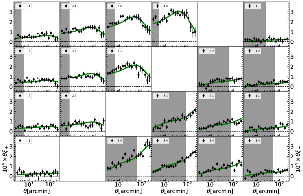
Figure 10: All auto correlations and cross correlations between different redshift bins. The green lines are the MTH prediction and its parameters are given in the column Planck+BAO+DES Y3+SZ (2013)+SH0ES of Table 4.

In Fig. 10, we show the full set of auto and cross two-point correlation functions of cosmic shear in each redshift bin. The top left corner is $\xi_{+}(\theta)$ while the bottom right corner is $\xi_{-}(\theta)$. The black data points in the plots are data from the DES Y3 METACALIBRATION shape catalog. The green solid lines denote the best-fit MTH model prediction with dataset Planck+BAO+DES Y3+SH0ES+SZ (2013) in Table 4. The error bars are the diagonal term of the covariance matrix described in Sec. 3.2.

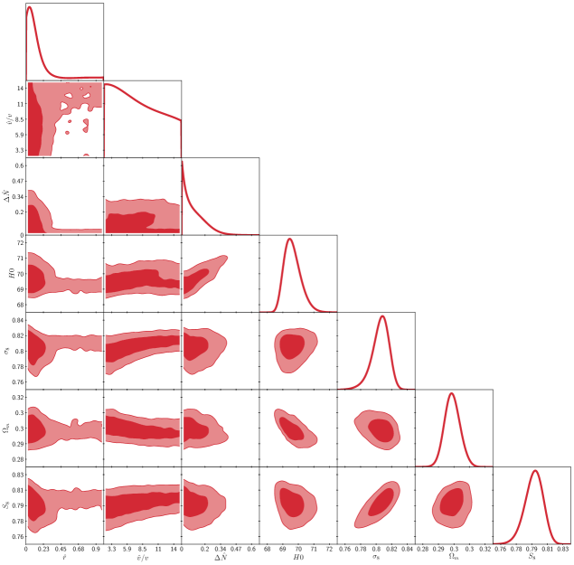
Figure 11: The triangle posterior distribution of MCMC results for the MTH model with dataset Planck+BAO+DES Y3.

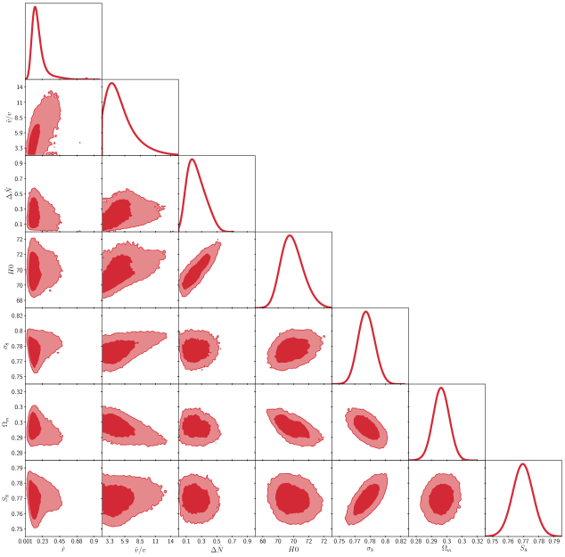
Figure 12: The triangle posterior distribution of MCMC results for the MTH model with dataset Planck+BAO+DES Y3+SH0ES+SZ (2013) experiments.

In Fig. 11 and Fig. 12, we show the triangle contour figures of the MTH model with datasets Planck+BAO+DES Y3 and Planck+BAO+DES Y3+SZ (2013)+SH0ES respectively.

References

- (1) Z. Chacko, H.-S. Goh and R. Harnik, The Twin Higgs: Natural electroweak breaking from mirror symmetry, Phys. Rev. Lett. 96 (2006) 231802, [hep-ph/0506256].
- (2) Z. Chacko, H.-S. Goh and R. Harnik, A Twin Higgs model from left-right symmetry, JHEP 01 (2006) 108, [hep-ph/0512088].
- (3) P. Ciarcelluti, Cosmology with mirror dark matter, Int. J. Mod. Phys. D 19 (2010) 2151–2230, [1102.5530].
- (4) P. Ciarcelluti, Cosmology with mirror dark matter. 1. Linear evolution of perturbations, Int. J. Mod. Phys. D 14 (2005) 187–222, [astro-ph/0409630].
- (5) P. Ciarcelluti, Cosmology with mirror dark matter. 2. Cosmic microwave background and large scale structure, Int. J. Mod. Phys. D 14 (2005) 223–256, [astro-ph/0409633].
- (6) DES collaboration, T. M. C. Abbott et al., Dark Energy Survey year 1 results: Cosmological constraints from galaxy clustering and weak lensing, Phys. Rev. D 98 (2018) 043526, [1708.01530].
- (7) DES collaboration, T. M. C. Abbott et al., Dark Energy Survey Year 3 results: Cosmological constraints from galaxy clustering and weak lensing, Phys. Rev. D 105 (2022) 023520, [2105.13549].
- (8) E. van Uitert et al., KiDS+GAMA: cosmology constraints from a joint analysis of cosmic shear, galaxy–galaxy lensing, and angular clustering, Mon. Not. Roy. Astron. Soc. 476 (2018) 4662–4689, [1706.05004].
- (9) C. Heymans et al., KiDS-1000 Cosmology: Multi-probe weak gravitational lensing and spectroscopic galaxy clustering constraints, Astron. Astrophys. 646 (2021) A140, [2007.15632].
- (10) HSC collaboration, C. Hikage et al., Cosmology from cosmic shear power spectra with Subaru Hyper Suprime-Cam first-year data, Publ. Astron. Soc. Jap. 71 (2019) 43, [1809.09148].
- (11) T. Hamana et al., Cosmological constraints from cosmic shear two-point correlation functions with HSC survey first-year data, Publ. Astron. Soc. Jap. 72 (2020) Publications of the Astronomical Society of Japan, Volume 72, Issue 1, February 2020, 16, https://doi.org/10.1093/pasj/psz138, [1906.06041].
- (12) LSST collaboration, v. Ivezić et al., LSST: from Science Drivers to Reference Design and Anticipated Data Products, Astrophys. J. 873 (2019) 111, [0805.2366].
- (13) EUCLID collaboration, R. Laureijs et al., Euclid Definition Study Report, 1110.3193.
- (14) J. Green et al., Wide-Field InfraRed Survey Telescope (WFIRST) Final Report, 1208.4012.
- (15) Z. Lou, M. Liang, D. Yao, X. Zheng, J. Cheng, H. Wang et al., Optical design study of the Wide Field Survey Telescope (WFST), in Advanced Optical Design and Manufacturing Technology and Astronomical Telescopes and Instrumentation (M. Xu and J. Yang, eds.), vol. 10154, p. 101542A, International Society for Optics and Photonics, SPIE, 2016, DOI.
- (16) L. Lei, Q.-F. Zhu, X. Kong, T.-G. Wang, X.-Z. Zheng, D.-D. Shi et al., Limiting Magnitudes of the Wide Field Survey Telescope (WFST), Res. Astron. Astrophys. 23 (2023) 035013, [2301.03068].
- (17) H. Zhan, Consideration for a large-scale multi-color imaging and slitless spectroscopy survey on the Chinese space station and its application in dark energy research, Scientia Sinica Physica, Mechanica & Astronomica 41 (Jan., 2011) 1441.
- (18) H. Zhan, The wide-field multiband imaging and slitless spectroscopy survey to be carried out by the survey space telescope of china manned space program, Chinese Science Bulletin 66 (04, 2021) 1290–1298.
- (19) Y. Gong, X. Liu, Y. Cao, X. Chen, Z. Fan, R. Li et al., Cosmology from the Chinese Space Station Optical Survey (CSS-OS), Astrophys. J. 883 (2019) 203, [1901.04634].
- (20) E. Di Valentino, O. Mena, S. Pan, L. Visinelli, W. Yang, A. Melchiorri et al., In the realm of the Hubble tension—a review of solutions, Class. Quant. Grav. 38 (2021) 153001, [2103.01183].
- (21) N. MacCrann, J. Zuntz, S. Bridle, B. Jain and M. R. Becker, Cosmic Discordance: Are Planck CMB and CFHTLenS weak lensing measurements out of tune?, Mon. Not. Roy. Astron. Soc. 451 (2015) 2877–2888, [1408.4742].
- (22) Planck collaboration, N. Aghanim et al., Planck 2018 results. VI. Cosmological parameters, Astron. Astrophys. 641 (2020) A6, [1807.06209].
- (23) A. G. Riess, S. Casertano, W. Yuan, J. B. Bowers, L. Macri, J. C. Zinn et al., Cosmic Distances Calibrated to 1% Precision with Gaia EDR3 Parallaxes and Hubble Space Telescope Photometry of 75 Milky Way Cepheids Confirm Tension with CDM, Astrophys. J. Lett. 908 (2021) L6, [2012.08534].
- (24) Y.-Y. Wang, S.-P. Tang, Z.-P. Jin and Y.-Z. Fan, The Late Afterglow of GW170817/GRB 170817A: A Large Viewing Angle and the Shift of the Hubble Constant to a Value More Consistent with the Local Measurements, Astrophys. J. 943 (2023) 13, [2208.09121].
- (25) Planck collaboration, N. Aghanim et al., Planck 2018 results. VIII. Gravitational lensing, Astron. Astrophys. 641 (2020) A8, [1807.06210].
- (26) H. Hildebrandt et al., KiDS+VIKING-450: Cosmic shear tomography with optical and infrared data, Astron. Astrophys. 633 (2020) A69, [1812.06076].
- (27) C. Krishnan, E. O. Colgáin, M. M. Sheikh-Jabbari and T. Yang, Running Hubble Tension and a H0 Diagnostic, Phys. Rev. D 103 (2021) 103509, [2011.02858].
- (28) S. A. Adil, O. Akarsu, M. Malekjani, E. O. Colgáin, S. Pourojaghi, A. A. Sen et al., increases with effective redshift in CDM cosmology, 2303.06928.
- (29) Planck collaboration, P. A. R. Ade et al., Planck 2013 results. XX. Cosmology from Sunyaev–Zeldovich cluster counts, Astron. Astrophys. 571 (2014) A20, [1303.5080].
- (30) A. von der Linden et al., Robust Weak-lensing Mass Calibration of Planck Galaxy Clusters, Mon. Not. Roy. Astron. Soc. 443 (2014) 1973–1978, [1402.2670].
- (31) K. Umetsu, Cluster–galaxy weak lensing, Astron. Astrophys. Rev. 28 (2020) 7, [2007.00506].
- (32) A. Blanchard and S. Ilić, Closing up the cluster tension?, Astron. Astrophys. 656 (2021) A75, [2104.00756].
- (33) R. C. Nunes and S. Vagnozzi, Arbitrating the S8 discrepancy with growth rate measurements from redshift-space distortions, Mon. Not. Roy. Astron. Soc. 505 (2021) 5427, [2106.01208].
- (34) J. Lesgourgues, G. Marques-Tavares and M. Schmaltz, Evidence for dark matter interactions in cosmological precision data?, JCAP 02 (2016) 037, [1507.04351].
- (35) Z. Chacko, Y. Cui, S. Hong, T. Okui and Y. Tsai, Partially Acoustic Dark Matter, Interacting Dark Radiation, and Large Scale Structure, JHEP 12 (2016) 108, [1609.03569].
- (36) R. Foot and S. Vagnozzi, Solving the small-scale structure puzzles with dissipative dark matter, JCAP 07 (2016) 013, [1602.02467].
- (37) M. A. Buen-Abad, M. Schmaltz, J. Lesgourgues and T. Brinckmann, Interacting Dark Sector and Precision Cosmology, JCAP 01 (2018) 008, [1708.09406].
- (38) Z. Chacko, D. Curtin, M. Geller and Y. Tsai, Cosmological Signatures of a Mirror Twin Higgs, JHEP 09 (2018) 163, [1803.03263].
- (39) C. Dessert, C. Kilic, C. Trendafilova and Y. Tsai, Addressing Astrophysical and Cosmological Problems With Secretly Asymmetric Dark Matter, Phys. Rev. D 100 (2019) 015029, [1811.05534].
- (40) S. Bansal, J. H. Kim, C. Kolda, M. Low and Y. Tsai, Mirror twin Higgs cosmology: constraints and a possible resolution to the H0 and S8 tensions, JHEP 05 (2022) 050, [2110.04317].
- (41) M. Joseph, D. Aloni, M. Schmaltz, E. N. Sivarajan and N. Weiner, A Step in Understanding the Tension, 2207.03500.
- (42) S. Bansal, J. Barron, D. Curtin and Y. Tsai, Precision Cosmological Constraints on Atomic Dark Matter, 2212.02487.
- (43) M. A. Buen-Abad, Z. Chacko, C. Kilic, G. Marques-Tavares and T. Youn, Stepped Partially Acoustic Dark Matter, Large Scale Structure, and the Hubble Tension, 2208.05984.
- (44) V. Poulin, T. L. Smith, T. Karwal and M. Kamionkowski, Early Dark Energy Can Resolve The Hubble Tension, Phys. Rev. Lett. 122 (2019) 221301, [1811.04083].
- (45) N. Schöneberg, G. Franco Abellán, A. Pérez Sánchez, S. J. Witte, V. Poulin and J. Lesgourgues, The H0 Olympics: A fair ranking of proposed models, Phys. Rept. 984 (2022) 1–55, [2107.10291].
- (46) L. A. Anchordoqui, E. Di Valentino, S. Pan and W. Yang, Dissecting the H0 and S8 tensions with Planck + BAO + supernova type Ia in multi-parameter cosmologies, JHEAp 32 (2021) 28–64, [2107.13932].
- (47) J. B. Muñoz, S. Bohr, F.-Y. Cyr-Racine, J. Zavala and M. Vogelsberger, ETHOS - an effective theory of structure formation: Impact of dark acoustic oscillations on cosmic dawn, Phys. Rev. D 103 (2021) 043512, [2011.05333].
- (48) S. Bohr, J. Zavala, F.-Y. Cyr-Racine, M. Vogelsberger, T. Bringmann and C. Pfrommer, ETHOS – an effective parametrization and classification for structure formation: the non-linear regime at z 5, Mon. Not. Roy. Astron. Soc. 498 (2020) 3403–3419, [2006.01842].
- (49) Planck collaboration, P. A. R. Ade et al., Planck 2015 results. XXIV. Cosmology from Sunyaev-Zeldovich cluster counts, Astron. Astrophys. 594 (2016) A24, [1502.01597].
- (50) DES collaboration, A. Amon et al., Dark Energy Survey Year 3 results: Cosmology from cosmic shear and robustness to data calibration, Phys. Rev. D 105 (2022) 023514, [2105.13543].
- (51) R. Foot, Mirror dark matter: Cosmology, galaxy structure and direct detection, Int. J. Mod. Phys. A 29 (2014) 1430013, [1401.3965].
- (52) Z. Chacko, D. Curtin, M. Geller and Y. Tsai, Direct detection of mirror matter in Twin Higgs models, JHEP 11 (2021) 198, [2104.02074].
- (53) L. Zu, G.-W. Yuan, L. Feng and Y.-Z. Fan, Mirror Dark Matter and Electronic Recoil Events in XENON1T, Nucl. Phys. B 965 (2021) 115369, [2006.14577].
- (54) D. Curtin and J. Setford, How To Discover Mirror Stars, Phys. Lett. B 804 (2020) 135391, [1909.04071].
- (55) D. Curtin and J. Setford, Signatures of Mirror Stars, JHEP 03 (2020) 041, [1909.04072].
- (56) Z. Chacko, N. Craig, P. J. Fox and R. Harnik, Cosmology in Mirror Twin Higgs and Neutrino Masses, JHEP 07 (2017) 023, [1611.07975].
- (57) N. Craig, S. Koren and T. Trott, Cosmological Signals of a Mirror Twin Higgs, JHEP 05 (2017) 038, [1611.07977].
- (58) H. Beauchesne and Y. Kats, Cosmology of the Twin Higgs without explicit 2 breaking, JHEP 12 (2021) 160, [2109.03279].
- (59) D. Blas, J. Lesgourgues and T. Tram, The Cosmic Linear Anisotropy Solving System (CLASS) II: Approximation schemes, JCAP 07 (2011) 034, [1104.2933].
- (60) F.-Y. Cyr-Racine, K. Sigurdson, J. Zavala, T. Bringmann, M. Vogelsberger and C. Pfrommer, ETHOS—an effective theory of structure formation: From dark particle physics to the matter distribution of the Universe, Phys. Rev. D 93 (2016) 123527, [1512.05344].
- (61) T. Schaeffer and A. Schneider, Dark acoustic oscillations: imprints on the matter power spectrum and the halo mass function, Mon. Not. Roy. Astron. Soc. 504 (2021) 3773–3786, [2101.12229].
- (62) A. Mead, C. Heymans, L. Lombriser, J. Peacock, O. Steele and H. Winther, Accurate halo-model matter power spectra with dark energy, massive neutrinos and modified gravitational forces, Mon. Not. Roy. Astron. Soc. 459 (2016) 1468–1488, [1602.02154].
- (63) DES collaboration, L. F. Secco et al., Dark Energy Survey Year 3 results: Cosmology from cosmic shear and robustness to modeling uncertainty, Phys. Rev. D 105 (2022) 023515, [2105.13544].
- (64) DES collaboration, M. A. Troxel et al., Dark Energy Survey Year 1 results: Cosmological constraints from cosmic shear, Phys. Rev. D 98 (2018) 043528, [1708.01538].
- (65) DES collaboration, M. Gatti et al., Dark energy survey year 3 results: weak lensing shape catalogue, Mon. Not. Roy. Astron. Soc. 504 (2021) 4312–4336, [2011.03408].
- (66) M. Jarvis, G. Bernstein and B. Jain, The skewness of the aperture mass statistic, Mon. Not. Roy. Astron. Soc. 352 (2004) 338–352, [astro-ph/0307393].
- (67) X. Fang, T. Eifler and E. Krause, 2D-FFTLog: Efficient computation of real space covariance matrices for galaxy clustering and weak lensing, Mon. Not. Roy. Astron. Soc. 497 (2020) 2699–2714, [2004.04833].
- (68) E. Krause and T. Eifler, cosmolike – cosmological likelihood analyses for photometric galaxy surveys, Mon. Not. Roy. Astron. Soc. 470 (2017) 2100–2112, [1601.05779].
- (69) D. N. Limber, The Analysis of Counts of the Extragalactic Nebulae in Terms of a Fluctuating Density Field. II, Astrophys. J. 119 (1954) 655.
- (70) M. LoVerde and N. Afshordi, Extended Limber Approximation, Phys. Rev. D 78 (2008) 123506, [0809.5112].
- (71) T. Brinckmann and J. Lesgourgues, MontePython 3: boosted MCMC sampler and other features, Phys. Dark Univ. 24 (2019) 100260, [1804.07261].
- (72) B. Audren, J. Lesgourgues, K. Benabed and S. Prunet, Conservative Constraints on Early Cosmology: an illustration of the Monte Python cosmological parameter inference code, JCAP 02 (2013) 001, [1210.7183].
- (73) Planck collaboration, N. Aghanim et al., Planck 2018 results. V. CMB power spectra and likelihoods, Astron. Astrophys. 641 (2020) A5, [1907.12875].
- (74) F. Beutler, C. Blake, M. Colless, D. H. Jones, L. Staveley-Smith, L. Campbell et al., The 6dF Galaxy Survey: Baryon Acoustic Oscillations and the Local Hubble Constant, Mon. Not. Roy. Astron. Soc. 416 (2011) 3017–3032, [1106.3366].
- (75) A. J. Ross, L. Samushia, C. Howlett, W. J. Percival, A. Burden and M. Manera, The clustering of the SDSS DR7 main Galaxy sample – I. A 4 per cent distance measure at , Mon. Not. Roy. Astron. Soc. 449 (2015) 835–847, [1409.3242].
- (76) BOSS collaboration, S. Alam et al., The clustering of galaxies in the completed SDSS-III Baryon Oscillation Spectroscopic Survey: cosmological analysis of the DR12 galaxy sample, Mon. Not. Roy. Astron. Soc. 470 (2017) 2617–2652, [1607.03155].
- (77) A. G. Riess et al., A Comprehensive Measurement of the Local Value of the Hubble Constant with 1 km s-1 Mpc-1 Uncertainty from the Hubble Space Telescope and the SH0ES Team, Astrophys. J. Lett. 934 (2022) L7, [2112.04510].
- (78) E. e. Abdalla, Cosmology intertwined: A review of the particle physics, astrophysics, and cosmology associated with the cosmological tensions and anomalies, Journal of High Energy Astrophysics 34 (June, 2022) 49–211, [2203.06142].
- (79) N. Craig, A. Katz, M. Strassler and R. Sundrum, Naturalness in the Dark at the LHC, JHEP 07 (2015) 105, [1501.05310].
- (80) D. Baumann, D. Green, J. Meyers and B. Wallisch, Phases of New Physics in the CMB, JCAP 01 (2016) 007, [1508.06342].
- (81) C. Brust, Y. Cui and K. Sigurdson, Cosmological Constraints on Interacting Light Particles, JCAP 08 (2017) 020, [1703.10732].
- (82) N. Blinov and G. Marques-Tavares, Interacting radiation after Planck and its implications for the Hubble Tension, JCAP 09 (2020) 029, [2003.08387].
- (83) S. Ghosh, S. Kumar and Y. Tsai, Free-streaming and coupled dark radiation isocurvature perturbations: constraints and application to the Hubble tension, JCAP 05 (2022) 014, [2107.09076].
- (84) T. Brinckmann, J. H. Chang, P. Du and M. LoVerde, Confronting interacting dark radiation scenarios with cosmological data, 2212.13264.
- (85) H. Rubira, A. Mazoun and M. Garny, Full-shape BOSS constraints on dark matter interacting with dark radiation and lifting the S8 tension, JCAP 01 (2023) 034, [2209.03974].
- (86) M. Raveri, W. Hu, T. Hoffman and L.-T. Wang, Partially Acoustic Dark Matter Cosmology and Cosmological Constraints, Phys. Rev. D 96 (2017) 103501, [1709.04877].
- (87) H. Lin, Y. Gong, X. Chen, K. C. Chan, Z. Fan and H. Zhan, Forecast of neutrino cosmology from the CSST photometric galaxy clustering and cosmic shear surveys, Mon. Not. Roy. Astron. Soc. 515 (2022) 5743–5757, [2203.11429].
- (88) V. Springel, The Cosmological simulation code GADGET-2, Mon. Not. Roy. Astron. Soc. 364 (2005) 1105–1134, [astro-ph/0505010].
- (89) M. Crocce, S. Pueblas and R. Scoccimarro, Transients from Initial Conditions in Cosmological Simulations, Mon. Not. Roy. Astron. Soc. 373 (2006) 369–381, [astro-ph/0606505].
- (90) K. L. Pandey, T. Karwal and S. Das, Alleviating the and anomalies with a decaying dark matter model, JCAP 07 (2020) 026, [1902.10636].
- (91) C. M. Hirata and U. Seljak, Intrinsic alignment-lensing interference as a contaminant of cosmic shear, Phys. Rev. D 70 (2004) 063526, [astro-ph/0406275].
- (92) S. Bridle and L. King, Dark energy constraints from cosmic shear power spectra: impact of intrinsic alignments on photometric redshift requirements, New J. Phys. 9 (2007) 444, [0705.0166].
- (93) B. Joachimi, R. Mandelbaum, F. B. Abdalla and S. L. Bridle, Constraints on intrinsic alignment contamination of weak lensing surveys using the MegaZ-LRG sample, Astron. Astrophys. 527 (2011) A26, [1008.3491].