High-performance descriptor for magnetic materials:
Accurate discrimination of magnetic structure

Abstract

The magnetic structure is crucial in determining the physical properties inherent in magnetic compounds. We present an adequate descriptor for magnetic structure with proper magnetic symmetry and high discrimination performance, which does not depend on artificial choices for coordinate origin, axis, and magnetic unit cell in crystal. We extend the formalism called “smooth overlap of atomic positions” (SOAP), providing a numerical representation of atomic configurations to that of magnetic moment configurations. We introduce the descriptor in terms of the vector spherical harmonics to describe a magnetic moment configuration and partial spectra from the expansion coefficients. We discuss that the lowest-order partial spectrum is insufficient to discriminate the magnetic structures with different magnetic anisotropy, and a higher-order partial spectrum is required in general to differentiate detailed magnetic structures on the same atomic configuration. We then introduce the fourth-order partial spectrum and evaluate the discrimination performance for different magnetic structures, mainly focusing on the difference in magnetic symmetry. The modified partial spectra that are defined not to reflect the difference of magnetic anisotropy are also useful in evaluating magnetic structures obtained from the first-principles calculations performed without spin-orbit coupling. We apply the present method to the symmetry-classified magnetic structures for the crystals of Mn₃Ir and Mn₃Sn, which are known to exhibit anomalous transport under the antiferromagnetic order, and examine the discrimination performance of the descriptor for different magnetic structures on the same crystal.

I INTRODUCTION

The recent significant advance in research using machine-learning techniques in quantum chemistry and condensed matter physics gets benefits from the development of high-performance descriptors that transform the structural information of molecules and crystals to data-style representations friendly to machine-learning applications. Various descriptors have been proposed for atomic configurations of molecules and crystals [1, 2, 3, 4, 5, 6, 7, 8] and applied to the analysis of nonmagnetic materials [9, 10].

For magnetic compounds, magnetic structure is crucial in determining their physical properties, and it must be taken into account as additional degrees of freedom in the descriptor. So far, only a few descriptors have been proposed to describe magnetic compounds, including the information on magnetic moments on each atomic site. “Moment Tensor Potentials,” “atomic symmetry functions,” and “Smooth Overlap of Atomic Positions (SOAP)” have been recently developed to encode the characters of magnetic materials [11, 12, 13]. These descriptors are applicable to distinguish different collinear magnetic structures, whose spin moments on each atomic site are parallel or anti-parallel, having either up or down-spin moments. However, in the more general cases including non-collinear magnetic structures, the descriptors must properly preserve the information on the directions of magnetic moments to analyze the macroscopic magnetic properties. The anomalous/topological Hall effect, nonreciprocal charge transport, and magnetoelectric effect are such examples, which are characterized by magnetic symmetry according to Neumann’s principle.

Domina et al. discuss a straightforward extension of the power spectrum of SOAP [5], in which the multi-dimensional vector is used to express atomic positions from the expansion coefficients of spherical harmonics for atomic density, and the power spectrum is calculated for magnetic configurations on atomic clusters [13]. However, as discussed in the present paper, the power spectrum calculated from the magnetization density is insufficient to characterize the magnetic structures on the high-symmetry atomic systems, and a higher-order partial spectrum is required to distinguish the magnetic structures with different magnetic symmetries. In this paper, we discuss four types of partial spectra, i.e., second and fourth-order partial spectra referred to as power spectrum and trispectrum, respectively, and those modified to neglect the difference of magnetic anisotropy in the magnetic structures and investigate the discrimination performance of those partial spectra for the high-symmetry magnetic structures. We also show that the modified partial spectra are useful in classifying the magnetic structures obtained from the first-principles calculations without considering the spin-orbit coupling.

The paper is organized as follows. Section II provides the formulation to transform the magnetic structure to partial spectra. In Sec. II.1, we define the magnetization density representing magnetic structures and provide the multipole expansion of the magnetization density with the explicit form of the expansion coefficients, as discussed in the literature [13]. In Sec. II.2, we derive the partial spectra from the second and higher-order similarity kernels defined by the overlap integral of different magnetic environments. In Sec. II.3, we discuss that the modified partial spectra that are defined not reflecting the difference in magnetic anisotropy. Section III discusses the discrimination performance of the magnetic structures on the same atomic configurations. In Sec. III.1, we discuss the basic behavior of partial spectra for the parameters introduced in the calculations by using magnetic configurations on a simple one-dimensional crystal structure. In Sec. III.2, the method is applied for the symmetrized magnetic structures classified according to the magnetic symmetries defined on the crystals of Mn₃Ir, which has a simple cubic structure, and Mn₃Sn, a hexagonal structure. The numerical tests for the magnetic compounds provide the knowledge of the appropriate choice of the derived magnetic partial spectra depending on magnetic environments. The new representation scheme of the magnetic moment configurations thus provides a solid foundation for machine learning, which is applicable to the study of magnetic materials, as summarized in Sec. IV.

II Formulation

This section provides formulations for transforming a given magnetic structure on the atomic cluster or crystal into a multi-dimensional vector. The outline of the procedure is, first, convert the magnetic moment configuration to a magnetization density and, second, expand the magnetization density by vector spherical harmonics with appropriate radial functions and, finally, construct the partial spectrum from the expansion coefficients in a similar way to obtain the partial spectrum from the expansion coefficients for the spherical harmonics expansion of the atomic density in SOAP [5]. We also introduce an averaging process for the magnetic partial spectra to eliminate dependencies on artificial choices of the coordinate origin in atomic clusters or crystals and discuss the appropriate methods.

II.1 Multipole expansion of local magnetic environment

Magnetic structures are usually represented by magnetic moment vectors with a certain order on discretely arranged atoms. To obtain the continuous vector function that characterizes the magnetic structure, we convert the magnetic moment configurations to the magnetization density by introducing the Gaussian function, choosing the coordinate’s origin at one of the atomic positions as follows:

$${\bm{m}}({\bm{r}})=\sum_{j=1}^{N}e^{-\alpha({\bm{r}}-{\bm{R}}_{j})^{2}}{\bm{m}}_{j}\ ,$$ (1)

where ${\bm{r}}$ is spatial position, ${\bm{R}}_{j}$ is the position of the $j$-th atom, ${\bm{m}}_{j}$ is the magnetic moment at the $j$-th atom, and $\alpha$=$\frac{1}{2\sigma^{2}}$ with a variance parameter $\sigma$.

The magnetization density is expanded with a set of vector spherical harmonics ${\bm{Y}}^{L}_{{\color[rgb]{0,0,0}\ell}m}(\hat{{\bm{r}}})$ (${\color[rgb]{0,0,0}\ell}\geq 1$, $-{\color[rgb]{0,0,0}\ell}\leq m\leq{\color[rgb]{0,0,0}\ell}$, $L={\color[rgb]{0,0,0}\ell}-1,{\color[rgb]{0,0,0}\ell},{\color[rgb]{0,0,0}\ell}+1$) and radial functions $\phi_{nl}(r)$ as

$${\bm{m}}({\bm{r}})=\sum_{nL{\color[rgb]{0,0,0}\ell}m}c_{nL{\color[rgb]{0,0,0}\ell}m}\phi_{n{\color[rgb]{0,0,0}\ell}}(r){\bm{Y}}^{L}_{{\color[rgb]{0,0,0}\ell}m}(\hat{{\bm{r}}})\ .$$ (2)

The vector spherical harmonics ${\bm{Y}}^{L}_{{\color[rgb]{0,0,0}\ell}m}$ are written with ordinary spherical harmonics $Y_{{\color[rgb]{0,0,0}\ell}m}({\bm{r}})$ and the Clebsh-Gordan coefficients $\braket{{\color[rgb]{0,0,0}\ell}_{1}m_{1};{\color[rgb]{0,0,0}\ell}_{2}m_{2}}{{\color[rgb]{0,0,0}\ell}_{3}m_{3}}$ as follows [14]:

$${\bm{Y}}^{L}_{{\color[rgb]{0,0,0}\ell}m}(\hat{{\bm{r}}})=\sum_{M=-L}^{L}\sum_{\sigma=-1}^{1}\braket{LM;1\sigma}{{\color[rgb]{0,0,0}\ell}m}Y_{LM}(\hat{{\bm{r}}}){\bm{e}}_{1\sigma}\ ,$$ (3)

where ${\bm{e}}_{1\sigma}$ are the spherical unit vectors satisfying the orthogonality relation ${\bm{e}}_{1\sigma}^{*}\cdot{\bm{e}}_{1\sigma^{\prime}}$=$\delta_{\sigma\sigma^{\prime}}$ and are expressed with the Cartesian unit vectors as follows:

$${\bm{e}}_{1-1} =\frac{1}{\sqrt{2}}({\bm{e}}_{x}-i{\bm{e}}_{y})$$

$${\bm{e}}_{10} ={\bm{e}}_{z}$$ (4)

$${\bm{e}}_{11} =-\frac{1}{\sqrt{2}}({\bm{e}}_{x}+i{\bm{e}}_{y})\ .$$

Since Clebsh-Gordan coefficients $\braket{{\color[rgb]{0,0,0}\ell}_{1}m_{1};{\color[rgb]{0,0,0}\ell}_{2}m_{2}}{{\color[rgb]{0,0,0}\ell}_{3}m_{3}}$ have finite values only if $m_{1}$+$m_{2}$=$m_{3}$, Eq. (3) is written as follows:

$${\bm{Y}}^{L}_{{\color[rgb]{0,0,0}\ell}m}(\hat{{\bm{r}}})=\sum_{\sigma=-1}^{1}\braket{L\,m\!-\!\sigma;1\,\sigma}{{\color[rgb]{0,0,0}\ell}\,m}Y_{Lm-\sigma}(\hat{{\bm{r}}}){\bm{e}}_{1\sigma}\ ,$$ (5)

where $\braket{L\,m\!-\!\sigma;1\,\sigma}{{\color[rgb]{0,0,0}\ell}\,m}=0$ for $\mid m-\sigma\mid>L$. The vector spherical harmonics have the orthogonality relation

$$\int d\Omega{\bm{Y}}_{{\color[rgb]{0,0,0}\ell}m}^{L{\color[rgb]{0,0,0}*}}(\widehat{{\bm{r}}})\cdot{\bm{Y}}_{{\color[rgb]{0,0,0}\ell}^{\prime}m^{\prime}}^{L^{\prime}}(\widehat{{\bm{r}}})=\delta_{LL^{\prime}}\delta_{{\color[rgb]{0,0,0}\ell\ell^{\prime}}}\delta_{mm^{\prime}}\ ,$$ (6)

from the relations ${\bm{e}}_{1\sigma}^{*}\cdot{\bm{e}}_{1\sigma^{\prime}}$=$\delta_{\sigma\sigma^{\prime}}$, $\int d\Omega Y_{\ell m}^{*}({\bm{r}})Y_{\ell^{\prime}m^{\prime}}({\bm{r}})=\delta_{\ell\ell^{\prime}}\delta_{mm^{\prime}}$, and the unitary relation $\sum_{M\sigma}\braket{{\color[rgb]{0,0,0}\ell}\,m\,}{LM;1\,\sigma}\braket{LM;1\,\sigma}{\ell^{\prime}\,m^{\prime}}=\delta_{\ell\ell^{\prime}}\delta_{mm^{\prime}}$. Eq. (3) is written with the Cartesian bases from Eq. (4), as follows:

$${\bm{Y}}^{L}_{{\color[rgb]{0,0,0}\ell}m}(\hat{{\bm{r}}}) =\sum_{\mu=x,y,z}\sum_{M=-L}^{L}C^{{\color[rgb]{0,0,0}\ell}m}_{LM\mu}Y_{LM}(\hat{{\bm{r}}}){\bm{e}}_{\mu}$$ (7)

where

$$C^{{\color[rgb]{0,0,0}\ell}m}_{LMx} =\frac{1}{\sqrt{2}}(\langle LM;1-1|{\color[rgb]{0,0,0}\ell}m\rangle-\braket{LM;11}{{\color[rgb]{0,0,0}\ell}m})$$

$$C^{{\color[rgb]{0,0,0}\ell}m}_{LMy} =\frac{-i}{\sqrt{2}}(\braket{LM;1-1}{{\color[rgb]{0,0,0}\ell}m}+\braket{LM;11}{{\color[rgb]{0,0,0}\ell}m})$$ (8)

$$C^{{\color[rgb]{0,0,0}\ell}m}_{LMz} =\braket{LM;10}{{\color[rgb]{0,0,0}\ell}m}$$

Some forms of radial functions $\phi_{n\ell}$ are suggested for the formula of SOAP in earlier works [5, 15]. We here adopt the radial functions suggested by Bartók et al. [5], which do not depend on angular momentum ${\color[rgb]{0,0,0}\ell}$, $\phi_{n{\color[rgb]{0,0,0}\ell}}=\phi_{n}$, and are orthonormalized in the range (0, $r_{\rm cut}$):

$$\int_{0}^{r_{\rm cut}}\phi_{n}(r)\phi_{n^{\prime}}(r)r^{2}dr=\delta_{nn^{\prime}}\ .$$ (9)

Considering the relation $e^{-\alpha({\bm{r}}+{\bm{R}}_{j})^{2}}$=$4\pi e^{-\alpha({\bm{r}}^{2}+{\bm{R}}_{j}^{2})}\sum_{{\color[rgb]{0,0,0}\ell}m}\mathcal{B}_{{\color[rgb]{0,0,0}\ell}}(2\alpha rR_{j})Y_{{\color[rgb]{0,0,0}\ell}m}(\widehat{{\bm{r}}})Y_{{\color[rgb]{0,0,0}\ell}m}^{*}(\widehat{{\bm{R}}_{j}})$ and the orthogonality relations of Eqs. (6) and (9), the expansion coefficients $c_{nL{\color[rgb]{0,0,0}\ell}m}$ in Eq. (2) are obtained from Eqs. (1) and (2) as follows:

$$c_{nL{\color[rgb]{0,0,0}\ell}m}=4\pi\int_{0}^{r_{\rm cut}}\sum_{j=1}^{N}\{e^{-\alpha(r^{2}+R_{j}^{2})}\mathcal{B}_{L}(2\alpha rR_{j}){\bm{Y}}_{{\color[rgb]{0,0,0}\ell}m}^{L*}(\hat{{\bm{R}}_{j}})\cdot{\bm{m}}_{j}\}\phi_{n}(r)r^{2}dr\ ,$$ (10)

where $\mathcal{B}_{L}$ is the modified Bessel function.

When the $i$-th atom located at the origin has a finite magnetic moment, the contribution from the central atom, $c^{(0)}_{nL{\color[rgb]{0,0,0}\ell}m}$, is included in Eq. (10) with $R_{j}=0$. From the modified Bessel functions $\mathcal{B}_{L}(R_{j}=0)=1$ for $L$=0 and 0 for $L\neq$0 and vector spherical harmonics ${\bm{Y}}_{00}^{0}$=${\bm{0}}$ and ${\bm{Y}}_{1m}^{0}$=$\sqrt{\frac{1}{4\pi}}{\bm{e}}_{1m}$, we obtain the analytic forms of the contribution from the central magnetic atom in Eq. (10) as:

$$c^{(0)}_{n01m}=\sqrt{4\pi}\int_{0}^{r_{\rm cut}}r^{2}\{e^{-\alpha r^{2}}{\bm{e}}_{1m}^{*}\cdot{\bm{m}}_{i}\}\phi_{n}(r)dr\ .$$ (11)

II.2 Partial spectra of local magnetic environment

Here, we derive the partial spectra of magnetization density, which are multiple-dimensional vectors characterizing the corresponding magnetic configuration. The basic procedure to derive the partial spectra is similar to those discussed in SOAP [5], except that we address the distribution of axial vectors, but there are some points to be noted. We define an overlap integral between two magnetization distributions ${\bm{m}}({\bm{r}})$ and ${\bm{m}}^{\prime}({\bm{r}})$ as follows:

$$S({\bm{m}},{\bm{m}}^{\prime})\equiv\int d{\bm{r}}{\bm{m}}^{*}({\bm{r}})\cdot{\bm{m}}^{\prime}({\bm{r}})\ .$$ (12)

The rotational invariants quantifying the similarity of the two magnetization densities are then obtained as follows:

$$k^{(\xi)}({\bm{m}},{\bm{m}}^{\prime})=\int d\hat{R}\mid S({\bm{m}},\hat{R}{\bm{m}}^{\prime})\mid^{\xi}\ ,$$ (13)

where $\hat{R}$ is the rotation operation. We refer to the quantity $k^{(\xi)}({\bm{m}},{\bm{m}}^{\prime})$ as $\xi$-th order similarity kernel of ${\bm{m}}$ and ${\bm{m}}^{\prime}$. We note that $k^{(\xi)}(\bm{m},\bm{m}^{\prime})$ in Eq. (13) for odd $\xi$, which may be defined such as $k^{(3)}({\bm{m}},{\bm{m}}^{\prime})=\int d\hat{R}S^{*}({\bm{m}},\hat{R}{\bm{m}}^{\prime})S({\bm{m}},\hat{R}{\bm{m}}^{\prime})S({\bm{m}},\hat{R}{\bm{m}}^{\prime})$, is always zero when the magnetic structure under consideration has, for instance, a two-fold rotation $\hat{R}_{2}$ symmetry satisfying $\hat{R}_{2}{\bm{m}}({\bm{r}})=-{\bm{m}}({\bm{r}})$ due to $S({\bm{m}},\hat{R}_{2}{\bm{m}}^{\prime})=-S({\bm{m}},{\bm{m}}^{\prime})$. $\hat{R}{\bm{m}}$ in Eq. (13) is calculated by using the transformation relation of the vector spherical harmonics for the rotation operation $R$ as:

$$\hat{R}{\bm{Y}}^{L}_{{\color[rgb]{0,0,0}\ell}m}=\sum_{m^{\prime}}{\bm{Y}}^{L}_{{\color[rgb]{0,0,0}\ell}m^{\prime}}D^{{\color[rgb]{0,0,0}\ell}}_{m^{\prime}m}(\hat{R})\ ,$$ (14)

where $D^{\ell}_{mm^{\prime}}$ is the matrix elements of the unitary representation matrix of the rotation operation for vector spherical harmonics, $D^{\ell}$, satisfying the relation

$$D^{{\color[rgb]{0,0,0}\ell}\dagger}(\hat{R})D^{{\color[rgb]{0,0,0}\ell}}(\hat{R})=I\ .$$ (15)

From Eqs. (2), (6), (9), and (14), the overlap integral in Eq. (13) is calculated as follows:

$$S({\bm{m}},\hat{R}{\bm{m}}^{\prime})=\sum_{nL\ell}\sum_{mm^{\prime}}c_{nL\ell m}^{*}c_{nL\ell m^{\prime}}^{\prime}D_{mm^{\prime}}^{\ell}(\hat{R})$$ (16)

We here introduce the inner product of the multi-dimensional vectors ${\bm{A}}$ and ${\bm{B}}$, whose complex components are identified by multiple indices as follows:

$$\braket{{\bm{A}},{\bm{B}}}=\sum_{\mu}A_{\mu}^{*}B_{\mu}\ ,$$ (17)

where $\mu$ represents all the indices specifying the components. The second-order similarity kernel of magnetization densities ${\bm{m}}$ and ${\bm{m}}^{\prime}$ is then obtained as

$$k^{(2)}({\bm{m}},{\bm{m}}^{\prime}) =\int d\hat{R}S^{*}({\bm{m}},\hat{R}{\bm{m}}^{\prime})S({\bm{m}},\hat{R}{\bm{m}}^{\prime})$$

$$=\sum_{nn^{\prime}}\sum_{LL^{\prime}}\sum_{\ell}(P_{nLn^{\prime}L^{\prime}\ell})^{*}P_{nLn^{\prime}L^{\prime}\ell}^{\prime}$$

$$=\braket{{\bm{P}},{\bm{P}}^{\prime}}\ ,$$ (18)

where ${\bm{P}}$ and ${\bm{P}}^{\prime}$ are considered vectors composed of the following elements:

$$P_{nLn^{\prime}L^{\prime}\ell} =\sqrt{\frac{8\pi^{2}}{2\ell+1}}\sum_{m}c^{*}_{nL\ell m}c_{n^{\prime}L^{\prime}\ell m}$$

$$=\sqrt{\frac{8\pi^{2}}{2\ell+1}}\braket{{\bm{c}}_{nL\ell},{\bm{c}}_{n^{\prime}L^{\prime}\ell}}\ .$$ (19)

To derive Eqs. (18) and (19), we used Eq. (16) and the relation

$$\int d\hat{R}D^{\ell_{1}*}_{m_{1}m_{1}^{\prime}}(\hat{R})D^{\ell_{2}}_{m_{2}m_{2}^{\prime}}(\hat{R})=\frac{8\pi^{2}}{2\ell_{1}+1}\delta_{\ell_{1}\ell_{2}}\delta_{m_{1}m_{2}}\delta_{m_{1}^{\prime}m_{2}^{\prime}}\ .$$ (20)

We refer to ${\bm{P}}$ (${\bm{P}}^{\prime}$) as a magnetic power spectrum for magnetization density ${\bm{m}}$ (${\bm{m}}^{\prime}$), which is similar to that defined for atomic densities [5]. As discussed after Eq. (13), the similarity kernel of Eq. (13) vanishes for odd $\xi$ when the magnetic structure has specific symmetry. Therefore, the bispectrum that can be derived from Eq. (13) for $\xi$=3, as discussed for SOAP in Ref. 5, is not appropriate as the descriptor of the magnetic structure. The fourth-order similarity kernel is also derived from Eq. (13) as follows:

$$k^{(4)}({\bm{m}},{\bm{m}}^{\prime}) =\int d\hat{R}\{S^{*}({\bm{m}},\hat{R}{\bm{m}}^{\prime})S({\bm{m}},\hat{R}{\bm{m}}^{\prime})\}^{2}$$

$$=\sum_{\gamma_{1}\gamma_{2}\gamma_{3}\gamma_{4}}\sum_{\ell=|\ell_{1}-\ell_{3}|}^{\ell_{1}+\ell_{3}}(T_{\gamma_{1}\gamma_{2}\gamma_{3}\gamma_{4}\ell})^{*}T^{\prime}_{\gamma_{1}\gamma_{2}\gamma_{3}\gamma_{4}\ell}$$

$$=\braket{{\bm{T}},{\bm{T}}^{\prime}}\ ,$$ (21)

where the multi-dimensional vector ${\bm{T}}$ (${\bm{T}}^{\prime}$), referred to as magnetic trispectrum, has the vector elements:

$$T_{\gamma_{1}\gamma_{2}\gamma_{3}\gamma_{4}\ell} =\sqrt{\frac{8\pi^{2}}{2\ell+1}}\sum_{m}{\color[rgb]{0,0,0}g_{\gamma_{1}\gamma_{2}\ell m}^{*}g_{\gamma_{3}\gamma_{4}\ell m}}$$

$$=\sqrt{\frac{8\pi^{2}}{2\ell+1}}\braket{{\bm{g}}_{\gamma_{1}\gamma_{2}\ell},{\bm{g}}_{\gamma_{3}\gamma_{4}\ell}}\ .$$ (22)

The $\gamma_{i}$ represents the set of $n_{i}$,$L_{i}$,${\color[rgb]{0,0,0}\ell}_{i}$, i.e., $\gamma_{i}$=$\{n_{i},L_{i},{\color[rgb]{0,0,0}\ell}_{i}\}$, and ${\color[rgb]{0,0,0}\ell}$ runs from $\max\{\mid{\color[rgb]{0,0,0}\ell}_{1}-{\color[rgb]{0,0,0}\ell}_{2}\mid,\mid{\color[rgb]{0,0,0}\ell}_{3}-{\color[rgb]{0,0,0}\ell}_{4}\mid\}$ to $\min\{{\color[rgb]{0,0,0}\ell}_{1}+{\color[rgb]{0,0,0}\ell}_{2},{\color[rgb]{0,0,0}\ell}_{3}+{\color[rgb]{0,0,0}\ell}_{4}\}$ and the vector elements of ${\bm{g}}_{\gamma_{1}\gamma_{2}{\color[rgb]{0,0,0}\ell}}$ are

$${\color[rgb]{0,0,0}g_{\gamma_{1}\gamma_{2}\ell m}}=\sum_{m^{\prime}}c_{\gamma_{1}m^{\prime}}c_{\gamma_{2}m\!-\!m^{\prime}}\braket{{\color[rgb]{0,0,0}\ell}_{1}m^{\prime};{\color[rgb]{0,0,0}\ell}_{2}m\!-\!m^{\prime}}{{\color[rgb]{0,0,0}\ell}m}\ ,$$ (23)

where $m$ takes integer values from $-{\color[rgb]{0,0,0}\ell}$ to ${\color[rgb]{0,0,0}\ell}$. To derive Eqs. (21)-(23), we used the relation

$$D^{\ell_{1}}_{m_{1}m_{1}^{\prime}}(\hat{R})D^{\ell_{2}}_{m_{2}m_{2}^{\prime}}(\hat{R})=$$

$$\sum_{\ell=|\ell_{1}-\ell_{2}|}^{\ell_{1}+\ell_{2}}\sum_{mm^{\prime}}\braket{\ell_{1}m_{1}\ell_{2}m_{2}}{\ell m} \braket{\ell_{1}m_{1}^{\prime}\ell_{2}m_{2}^{\prime}}{\ell m^{\prime}}D^{\ell}_{mm^{\prime}}(\hat{R})$$ (24)

in addition to Eqs. (16) and (20).

The name ”trispectrum” for the quantity of Eq. (22) is taken after a terminology in signal theory, as similar to ”power spectrum” and ”bispectrum” [16]. As discussed in Sec. III.2, a higher-order partial spectrum is necessary to distinguish the magnetic structures given by the same atomic configuration, for instance, magnetic structures only with different magnetic anisotropies.

II.3 Modified partial spectrum irrespective of magnetic anisotropy

In the derivation of the partial spectra in the previous subsections, it was assumed that the magnetic moments rotate in accordance with the spatial rotation of the crystal. The coupling between crystal axes and magnetic moment is realized through the spin-orbit interaction, which is a relativistic effect. Meanwhile, first-principles calculations for magnetic systems are often implemented without taking spin-orbit interaction to make the calculations faster or to understand the magnetic states with the simplified picture of the spin space. In the absence of spin-orbit interaction, the rotation of magnetic moments and crystal axes can be performed independently. As a result, magnetic structures arising from rotations in spin have the same total energy.

It is thus useful to introduce the modified partial spectrum representation, which does not distinguish the magnetic structures only with different magnetic anisotropy. To obtain such a partial spectrum, we expand the magnetization density with the product function of the normal spherical harmonics and the unit vector as the bases of the classical spin space as

$${\bm{m}}({\bm{r}})=\sum_{n{\color[rgb]{0,0,0}\ell}m\sigma}\overline{c}_{n{\color[rgb]{0,0,0}\ell}m\sigma}\phi_{n}(r)Y_{{\color[rgb]{0,0,0}\ell}m}(\hat{{\bm{r}}}){\bm{e}}_{1\sigma}\ .$$ (25)

From Eqs. (1) and (25), the expansion coefficients $\overline{c}_{n{\color[rgb]{0,0,0}\ell}m\sigma}$ are calculated as follows:

$$\overline{c}_{n{\color[rgb]{0,0,0}\ell}m\sigma}=4\pi\int_{0}^{r_{\rm cut}}\sum_{j}^{N}\{e^{-\alpha(r^{2}+R_{j}^{2})}\mathcal{B}_{{\color[rgb]{0,0,0}\ell}}(2\alpha rR_{j})Y_{{\color[rgb]{0,0,0}\ell}m}^{*}(\hat{{\bm{R}}_{j}}){\bm{e}}^{*}_{1\sigma}\cdot{\bm{m}}_{j}\}\phi_{n}(r)r^{2}dr\ .$$ (26)

The contribution from the $i$-th magnetic atom located at the origin with $R_{j}=0$, $\overline{c}^{(0)}_{n{\color[rgb]{0,0,0}\ell}m\sigma}$, in Eq.(26) is finite only for ${\color[rgb]{0,0,0}\ell}$=$m$=$0$ and has the analytic form as follows:

$$\overline{c}^{(0)}_{n00\sigma}=\sqrt{4\pi}\int_{0}^{r_{\rm cut}}r^{2}\{e^{-\alpha r^{2}}{\bm{e}}_{1\sigma}^{*}\cdot{\bm{m}}_{i}\}\phi_{n}(r)dr\ .$$ (27)

The magnetic structures only with different magnetic anisotropy are transformed with each other through a rotation of the spin moments only in the spin space. Therefore, the partial spectra to characterize magnetic moment configurations irrespective of magnetic anisotropy are given by the following similarity kernel:

$$\overline{k}^{(\xi)}({\bm{m}},{\bm{m}}^{\prime})=\int d{\color[rgb]{0,0,0}\hat{R}}\int d{\color[rgb]{0,0,0}\hat{R}_{s}}\mid S({\bm{m}},{\color[rgb]{0,0,0}\hat{R}\hat{R}_{s}}{\bm{m}}^{\prime})\mid^{\xi}\ ,$$ (28)

where the rotation operator for magnetization density now works separately for the spatial coordinate ($R$) and spin coordinate ($R_{s}$) as follows:

$${\color[rgb]{0,0,0}\hat{R}\hat{R}_{s}}{\bm{m}}({\bm{r}})=\sum_{n{\color[rgb]{0,0,0}\ell}m\sigma}\overline{c}_{n{\color[rgb]{0,0,0}\ell}m\sigma}\phi_{n}(r)\sum_{m^{\prime}\sigma^{\prime}}Y_{{\color[rgb]{0,0,0}\ell}m^{\prime}}{\bm{e}}_{1\sigma^{\prime}}D^{{\color[rgb]{0,0,0}\ell}}_{m^{\prime}m}(\hat{R})D^{s}_{\sigma^{\prime}\sigma}(\hat{R}_{s}).$$ (29)

Eq. (28) leads to the power spectrum for $\xi$=2 as:

$$\overline{P}_{nn^{\prime}{\color[rgb]{0,0,0}\ell}}=\sqrt{\frac{8\pi^{2}}{2{\color[rgb]{0,0,0}\ell}+1}}\sqrt{\frac{8\pi^{2}}{3}}\braket{\overline{{\bm{c}}}_{n{\color[rgb]{0,0,0}\ell}},\overline{{\bm{c}}}_{n^{\prime}{\color[rgb]{0,0,0}\ell}}}\ ,$$ (30)

and the trispectrum for $\xi$=4:

$$\overline{T}_{n_{1}{\color[rgb]{0,0,0}\ell}_{1}n_{2}{\color[rgb]{0,0,0}\ell}_{2}n_{3}{\color[rgb]{0,0,0}\ell}_{3}n_{4}{\color[rgb]{0,0,0}\ell}_{4}}^{{\color[rgb]{0,0,0}\ell}j}=\sqrt{\frac{8\pi^{2}}{2{\color[rgb]{0,0,0}\ell}+1}}\sqrt{\frac{8\pi^{2}}{2j+1}}\braket{\overline{{\bm{g}}}_{n_{1}{\color[rgb]{0,0,0}\ell}_{1}n_{2}{\color[rgb]{0,0,0}\ell}_{2}}^{{\color[rgb]{0,0,0}\ell}j},\overline{{\bm{g}}}_{n_{3}{\color[rgb]{0,0,0}\ell}_{3}n_{4}{\color[rgb]{0,0,0}\ell}_{4}}^{{\color[rgb]{0,0,0}\ell}j}}\ ,$$ (31)

where

$${\color[rgb]{0,0,0}\overline{g}^{\ell j}_{n_{1}\ell_{1}n_{2}\ell_{2}m\sigma}}=\sum_{m^{\prime}=-{\color[rgb]{0,0,0}\ell}}^{{\color[rgb]{0,0,0}\ell}}\sum_{\sigma^{\prime}=-j}^{j}\overline{c}_{n{\color[rgb]{0,0,0}\ell}m^{\prime}\sigma^{\prime}}\overline{c}_{n^{\prime}{\color[rgb]{0,0,0}\ell}^{\prime}m\!-\!m^{\prime}\sigma\!-\!\sigma^{\prime}}\braket{{\color[rgb]{0,0,0}\ell}_{1}m^{\prime};{\color[rgb]{0,0,0}\ell}_{2}m\!-\!m^{\prime}}{{\color[rgb]{0,0,0}\ell}m}\braket{1\sigma^{\prime};1\sigma\!-\!\sigma^{\prime}}{j\sigma}\ ,$$ (32)

where $\ell$ runs from $|{\color[rgb]{0,0,0}\ell}_{1}\!-\!{\color[rgb]{0,0,0}\ell}_{2}|$ to ${\color[rgb]{0,0,0}\ell}_{1}\!+\!{\color[rgb]{0,0,0}\ell}_{2}$ and $j$ from 0 to 2.

II.4 Elimination of origin choice dependency

As a descriptor, the magnetic partial spectrum should not depend on the artificial choices of the origin of the coordinate in the atomic system. To eliminate the origin choice dependency of the magnetic partial spectra in Sec. II.2 and II.3, we redefine the partial spectra by taking the average of the expansion coefficients over origin choices at all atoms in the atomic cluster or the crystal’s unit cell. The average of atomic positions can be applied directly for the expansion coefficients ${\bm{c}}^{i}_{nL{\color[rgb]{0,0,0}\ell}}$, where $i$ indicates the atomic site chosen as the coordinate’s origin, similar to the partial power spectrum for atomic positions [5], such as

$$P_{nLn^{\prime}L^{\prime}{\color[rgb]{0,0,0}\ell}}^{({\rm in})} =\sqrt{\frac{8\pi^{2}}{2{\color[rgb]{0,0,0}\ell}+1}}\frac{1}{N^{2}}\braket{\biggl{(}\sum_{i=1}^{N}{\bm{c}}^{i}_{nL{\color[rgb]{0,0,0}\ell}}\biggr{)},\biggl{(}\sum_{j=1}^{N}{\bm{c}}^{j}_{n^{\prime}L^{\prime}{\color[rgb]{0,0,0}\ell}}\biggr{)}}\ ,$$ (33)

$$T_{\gamma_{1}\gamma_{2}\gamma_{3}\gamma_{4}{\color[rgb]{0,0,0}\ell}}^{({\rm in})} =\sqrt{\frac{8\pi^{2}}{2{\color[rgb]{0,0,0}\ell}+1}}\frac{1}{N^{2}}\braket{(\sum_{i=1}^{N}{\bm{g}}_{\gamma_{1}\gamma_{2}{\color[rgb]{0,0,0}\ell}}^{i}),(\sum_{j=1}^{N}{\bm{g}}^{j}_{\gamma_{3}\gamma_{4}{\color[rgb]{0,0,0}\ell}})}\ {\color[rgb]{0,0,0},}$$ (34)

where $N$ is the number of atoms in the atomic cluster or the crystal’s unit cell. One other way of origin-choice average over the atomic positions for the product of the expansion coefficients is given as follows:

$$P_{nLn^{\prime}L^{\prime}{\color[rgb]{0,0,0}\ell}}^{({\rm out})} =\sqrt{\frac{8\pi^{2}}{2{\color[rgb]{0,0,0}\ell}+1}}\frac{1}{N}\sum_{i=1}^{N}\braket{{\bm{c}}^{i}_{nL{\color[rgb]{0,0,0}\ell}},{\bm{c}}^{i}_{n^{\prime}L^{\prime}{\color[rgb]{0,0,0}\ell}}}\ ,$$ (35)

$$T_{\gamma_{1}\gamma_{2}\gamma_{3}\gamma_{4}{\color[rgb]{0,0,0}\ell}}^{({\rm out})} =\sqrt{\frac{8\pi^{2}}{2{\color[rgb]{0,0,0}\ell}+1}}\frac{1}{N}\sum_{i=1}^{N}\braket{{\bm{g}}_{\gamma_{1}\gamma_{2}{\color[rgb]{0,0,0}\ell}}^{i},{\bm{g}}^{i}_{\gamma_{3}\gamma_{4}{\color[rgb]{0,0,0}\ell}}}\ .$$ (36)

We refer to the average implemented in Eq. (33) and (34) as the inner average and those in Eq. (35) and Eq. (36) as the outer average.

The inner average for the power spectrum can be zero for specific magnetic structures, such as the typical antiferromagnetic configuration whose magnetic moments are alternating on each sub-lattice. Hereafter, we take the outer average for the power spectrum and the inner average for the trispectrum. This redefines the second- and fourth-order similarity kernels with the power spectrum ${\bm{P}}$ and trispectrum ${\bm{T}}$ as follows:

$$k^{(2)}({\bm{m}},{\bm{m}}^{\prime}) =\sum_{nn^{\prime}}\sum_{LL^{\prime}}\sum_{\ell}(P_{nLn^{\prime}L^{\prime}\ell}^{({\rm out})})^{*}P_{nLn^{\prime}L^{\prime}\ell}^{\prime({\rm out})}$$

$$=\braket{{\bm{P}},{\bm{P}}^{\prime}}\ ,$$ (37)

$$k^{(4)}({\bm{m}},{\bm{m}}^{\prime}) =\sum_{\gamma_{1}\gamma_{2}\gamma_{3}\gamma_{4}}\sum_{\ell=|\ell_{1}-\ell_{3}|}^{\ell_{1}+\ell_{3}}(T_{\gamma_{1}\gamma_{2}\gamma_{3}\gamma_{4}\ell}^{({\rm in})})^{*}T_{\gamma_{1}\gamma_{2}\gamma_{3}\gamma_{4}\ell}^{\prime({\rm in})}$$

$$=\braket{{\bm{T}},{\bm{T}}^{\prime}}$$ (38)

As discussed in Sec. III, the power spectrum ${\bm{P}}$ is insufficient to fully distinguish magnetic structures with distinct magnetic symmetries in the same atomic configuration, and a higher-order spectrum is necessary to distinguish such magnetic structures through the overlap of magnetization densities at different atomic sites.

III Numerical results

In this section, we demonstrate the parameter dependence and discrimination performance of the magnetic partial spectra derived in Sec. II for the magnetic structures in high-symmetry crystals. To measure the similarity of magnetization density, we use the normalized similarity kernels defined as follows:

$$K^{(2)}({\bm{m}},{\bm{m}}^{\prime})=\frac{\braket{{\bm{P}},{\bm{P}}^{\prime}}}{\sqrt{\braket{{\bm{P}},{\bm{P}}}}\sqrt{\braket{{\bm{P}}^{\prime},{\bm{P}}^{\prime}}}}\ ,$$ (39)

$$K^{(4)}{\color[rgb]{0,0,0}({\bm{m}},{\bm{m}}^{\prime})}=\frac{\braket{{\bm{T}},{\bm{T}}^{\prime}}}{\sqrt{\braket{{\bm{T}},{\bm{T}}}}\sqrt{\braket{{\bm{T}}^{\prime},{\bm{T}}^{\prime}}}}\ ,$$ (40)

where ${\bm{P}}$ (${\bm{P}}^{\prime}$) and ${\bm{T}}$ (${\bm{T}}^{\prime}$) are the power spectrum and trispectrum for the magnetization density ${\bm{m}}$ (${\bm{m}}^{\prime}$). We also define the normalized similarity kernels irrespective of magnetic anisotropy by using $\overline{\bm{P}}$, $\overline{\bm{P}}^{\prime}$, $\overline{\bm{T}}$, $\overline{\bm{T}}^{\prime}$, derived in Sec. II.3, instead of ${\bm{P}}$, ${\bm{P}}^{\prime}$, ${\bm{T}}$, ${\bm{T}}^{\prime}$ in Eqs. (39) and (40) as $\overline{K}^{(2)}({\bm{m}},{\bm{m}}^{\prime})$ and $\overline{K}^{(4)}({\bm{m}},{\bm{m}}^{\prime})$, respectively.

These similarity kernels take the positive value in the range $[0,1]$ since the similarity kernel is derived from Eq. (13) or (28) with even $\xi$. We have implemented the calculations of SOAP with magnetic alignment by modifying the Python library, DScribe [15].

III.1 Parameter dependence of the similarity kernels

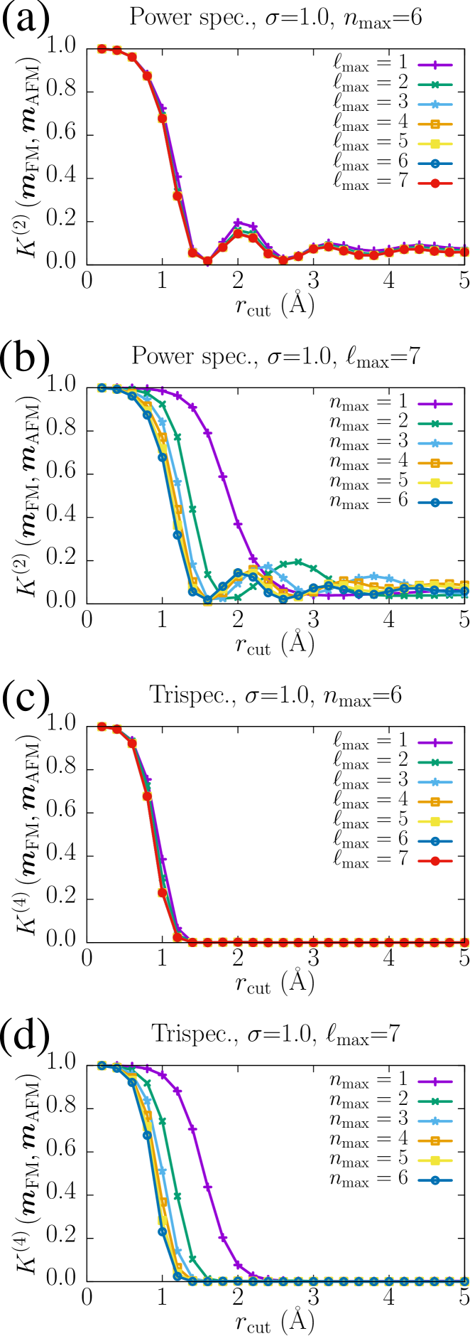
Figure 1: The $r_{\rm cut}$ dependence of the similarity kernels for the ferromagnetic (FM) and antiferromagnetic (AFM) systems. Panels (a)-(d) show the $K^{(2)}$ and $K^{(4)}$ values as a function of ${\color[rgb]{0,0,0}\ell}_{\rm max}$ with fixed $n_{\rm max}=6$ or $n_{\rm max}$ with fixed ${\color[rgb]{0,0,0}\ell}_{\rm max}=7$. The magnetic moments are ordered along the $z$-axis on each atomic site in the one-dimensional periodic lattice with 1 Å interval along the $x$-axis.

In this section, we discuss how the similarity kernel $K^{(2)}$ and $K^{(4)}$, defined by Eq. (39) with the power spectrum $\bm{P}$ and (40) with the trispectrum $\bm{T}$, respectively, behave in the application for magnetic configurations on simple crystals. Note that $K^{(2)}$ and $K^{(4)}$ contain four parameters: the width of the magnetization distribution $\sigma$ (i.e., $\alpha$), the number of radial basis functions $n_{\rm max}$, the maximum angular momentum of the vector spherical harmonics ${\color[rgb]{0,0,0}\ell}_{\rm max}$, and $r_{\rm cut}$ as the cutoff for the radial integration in Eq. (10). We will discuss these parameter dependences of $K^{(2)}$ and $K^{(4)}$ and show that $n_{\rm max}$ and ${\color[rgb]{0,0,0}\ell}_{\rm max}$ need to be sufficiently large to achieve convergence, while appropriate values for $\sigma$ and $r_{\rm cut}$ must be chosen according to an individual purpose.

Let us first discuss the simplest case, a one-dimensional chain with spins placed at intervals of 1 Å along the $x$-axis, and consider the similarity kernel between the FM and AFM ordered systems. In Fig. 1, we show the similarity kernels $K^{(2)}$ and $K^{(4)}$. Here, we fix the two pairs of parameters, namely, $\sigma$ and $n_{\rm max}$ ((a) and (c)), and $\sigma$ and ${\color[rgb]{0,0,0}\ell}_{\rm max}$ ((b) and (d)), and change other parameters. In all cases, $K^{(2)}$ and $K^{(4)}$ converge as $n_{\rm max}$ or ${\color[rgb]{0,0,0}\ell}_{\rm max}$ become larger. The convergence is faster for ${\color[rgb]{0,0,0}\ell}_{\rm max}$ than for $n_{\rm max}$ since we are working with a one-dimensional chain where angular dependence is less significant. On the other hand, $K^{(2)}$ and $K^{(4)}$ change from 1 to 0 as $r_{\rm cut}$ increases. This can be understood from Eq. (10), which suggests that a small $r_{\rm cut}$ including only one spin in the region cannot distinguish the FM and AFM states. Here, $K^{(2)}$ and $K^{(4)}$ show almost the same $r_{\rm cut}$ dependence, with the only difference being that $K^{(4)}$ approaches zero faster than $K^{(2)}$.

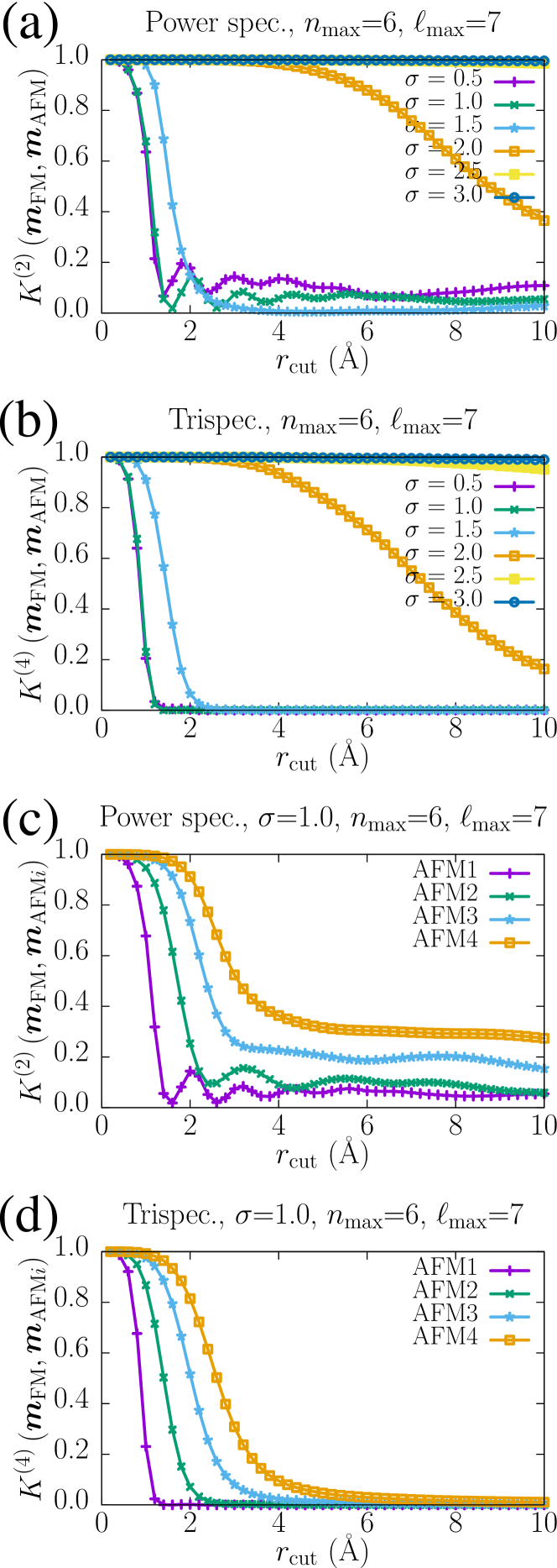
Figure 2: Similarity kernels with different values of $\sigma$, using $n_{\rm max}$=6 and ${\color[rgb]{0,0,0}\ell}_{\rm max}$=7 for FM and AFM configurations on the one-dimensional crystal, (a) $K^{(2)}$ and (b) $K^{(4)}$. Panels (c) and (d) compare the similarity kernels for FM and different AFM$i$ magnetic patterns, where the magnetic moments have opposite signs per $i$-atomic sites. $\sigma=1.0$Å, $n_{\rm max}$=6, and ${\color[rgb]{0,0,0}\ell}_{\rm max}$=7 are used.

Figures 2(a) and (b) show the $\sigma$ and $r_{\rm cut}$ dependence of $K^{(2)}$ and $K^{(4)}$, respectively, with converged values of ${\color[rgb]{0,0,0}\ell}_{\rm max}$ and $n_{\rm max}$. We can see that increasing $\sigma$ shifts the crossover point between the FM and AFM states to larger values of $r_{\rm cut}$. In the large $\sigma$ limit, $K^{(2)}\sim K^{(4)}\sim 1$ regardless of the value of $r_{\rm cut}$. This is reasonable with Eqs. (10), as well as Eqs. (39) and  (40). Namely, $e^{-\alpha(\bm{r}+\bm{R}_{j})^{2}}$ factor becomes constant in the large $\sigma$ limit, resulting in a constant factor change depending on the magnetic structure. As this constant change is lost in the normalization in Eqs. (39) and  (40), the resulting $K$ shows no distinction between FM and AFM configurations. These findings imply that the appropriate choice of $\sigma$ and $r_{\rm cut}$ is needed for the magnetic partial spectra to get meaningful information about the magnetic structure. To get more insight, we show the normalized similarity kernels, $K^{(2)}$ and $K^{(4)}$, between the FM order and several AFM orders in Figs. 2 (c) and (d). Here, AFM1, AFM2, AFM3, and AFM4 correspond to $\uparrow\downarrow$, $\uparrow\uparrow\downarrow\downarrow$, $\uparrow\uparrow\uparrow\downarrow\downarrow\downarrow$, and $\uparrow\uparrow\uparrow\uparrow\downarrow\downarrow\downarrow\downarrow$ periodic magnetic structures, respectively, in the one-dimensional crystal. Obviously, AFM4 is closer to FM than AFM3, while AFM1 is the farthest from FM, indicating that accurate discrimination among these states is crucial when comparing similarity with FM. When we use $\sigma$=1.0Å, as shown in Fig. 2(c) and (d), the four states can be distinguished by using $r_{\rm cut}\sim 3$ with $K^{(2)}$. In contrast, with trispectrum, $K^{(4)}$, the differences between the four states are relatively small compared to $K^{(2)}$ for large $r_{\rm cut}$, but they can still be distinguishable. The results indicate that the power spectrum is a better descriptor than the trispectrum for this specific purpose, as it allows for more apparent discrimination of these magnetic configurations.

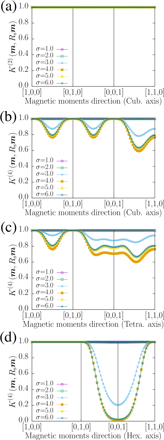
Figure 3: The spin rotation dependence of the normalized similarity kernels between the magnetization density of the ferromagnetic structure along the (100)-axis, denoted by ${\bm{m}}$, and those of the rotated magnetic moments, given by $R_{s}(\theta,\phi){\bm{m}}$. The results are presented for (a)$K^{(2)}$ and (b) $K^{(4)}$ on a simple BCC lattice with lattice constant $a$=1.0Å, (c) $K^{(4)}$ on a body center tetragonal lattice with $a$=1.0Å and $c$=1.5Å, and (d) $K^{(4)}$ on a hexagonal lattice with $a$=1.0Å and $c$=1.5Å, using $n_{\rm max}$=4, ${\color[rgb]{0,0,0}\ell}_{\rm max}$=6, and $r_{\rm cut}$=5.0Å.

Based on these results, we propose the following strategies for determining appropriate values of $r_{\rm cut}$ and $\sigma$:

• First, set $r_{\rm cut}$ depending on the purpose. For example, when classifying the magnetic structures, $r_{\rm cut}$ should be chosen based on their typical spatial scale to be distinguished.

• Then, $\sigma$ should be chosen so that the most distinct typical magnetic structures realized within the chosen $r_{\rm cut}$, such as the conventional FM and AFM states, approach $K\sim 0$.

Up to now, $K^{(2)}$ and $K^{(4)}$ do not show a significant difference. However, for the purpose of distinguishing the magnetic structures with different magnetic symmetries, we will show that $K^{(4)}$ would be a better descriptor than $K^{(2)}$.

Figure 3 displays the angle dependence of the similarity kernels between simple ferromagnetic orders along the $x$-axis and different directions of magnetic moments in polar coordinates $(\theta,\phi)$ on a simple body center cubic, tetragonal, and hexagonal lattices with their origin $(\theta=0,\phi=0)$ set to the $x$-axis. In all crystal systems, the crystal $a$-axis is set to 1 Å, and the $c$-axis of tetragonal and hexagonal lattices is set to 1.5Å. The plots show that, while the second-order similarity kernels $K^{(2)}$ do not show any difference for the magnetic anisotropy, the similarity kernel $K^{(4)}$ captures the difference from magnetic anisotropy. Note that the difference is captured through the overlap of the magnetization density around neighboring atoms since some extent of $\sigma$ is required to capture the difference of magnetic anisotropy, as shown in Fig. 3. As shown in the following subsection, $K^{(4)}$ has better discrimination performance than $K^{(2)}$ for magnetic anisotropy, though $K^{(2)}$ is not entirely useless for differentiating magnetic structures that differ only in magnetic anisotropy.

Note that the modified partial spectra insensitive to magnetic anisotropy are designed not to reflect the anisotropy difference even for the higher-order partial spectra. As a result, $\overline{K}^{(2)}$ and $\overline{K}^{(4)}$ both show 1.0 for any ($\theta$, $\phi$) as well as the plots of $K^{(2)}$ in Fig. 3 (a). The difference of the magnetic anisotropy for the rotation along the $z$-axis for the hexagonal lattice is not reflected even for the fourth-order partial spectrum $K^{(4)}$, as shown in Fig. 3 (d), implying that the magnetic partial spectrum with the order higher than four is necessary to capture such a difference. Differentiating magnetic anisotropy is essential for classifying magnetic symmetries of the magnetic alignments on the same atomic configurations, as discussed in Sec. III.2.

III.2 Discrimination performance for magnetic structures with distinct magnetic symmetries

Magnetic symmetries of the magnetic systems determine whether or not various physical properties of magnetic materials occur, such as anomalous Hall and Nernst effect, electromagnetic effect, and magnetic Kerr effect. The ability to distinguish different magnetic symmetries of a descriptor is thus crucial to analyze the physical properties of magnetic materials by using machine learning.

Although the expansion coefficients $c_{nLlm}$ of the vector spherical harmonics for magnetization density in Eq. (2) contain all information on magnetic environments, some information may be lost through the procedure of constructing the partial spectra from the expansion coefficients. To examine the ability to capture magnetic symmetry in the current scheme, we investigate the similarity kernels for the magnetic structures classified according to the symmetries of magnetic structures in high symmetry crystals, cubic Mn₃Ir and hexagonal Mn₃Sn. The crystal structures of Mn₃Ir and Mn₃Sn belong to the space group $Pm\overline{3}m$ ($O_{h}^{1}$, No.221), and $P6_{3}/mmc$ ($D_{6h}^{4}$, No.194), respectively. The lattice constants are $a$=3.77 Å for Mn₃Ir and $a$=5.665Å and $c$=4.531Å for Mn₃Sn. The magnetic structures of Mn₃Ir and Mn₃Sn, which are classified according to the irreducible representations of their respective crystal point groups ($O_{h}$ for cubic Mn₃Ir and $D_{6h}$ for hexagonal Mn₃Sn), were generated using the cluster multipole method described in Ref. 17. With the method, the magnetic structure bases classified by multipoles symmetrized according to the irreducible representations of the crystallographic point group are systematically generated by first generating magnetic structures on virtual atomic clusters belonging to the point group that conforms to the multipole moments symmetrized according to the point group, and then mapping them onto atoms in the crystal in a way that preserves convertibility with respect to the point group operations [17]. For Mn₃Ir, the magnetic structures with different magnetic symmetries within the same multipoles are produced by taking the linear combination of the generated magnetic bases as explained in Ref. 18. In each magnetic structure, the size of the magnetic moment was normalized to one at each magnetic site. The symmetrized magnetic structures for cubic Mn₃Ir and hexagonal Mn₃Sn are shown in Fig.4 and Fig.5, respectively. Additional details regarding the crystal and magnetic structures can be found in the Supplementary Information.

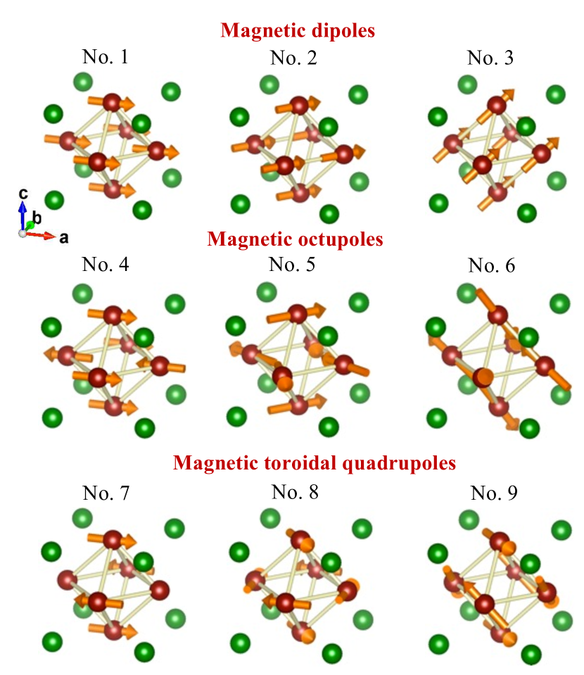
Figure 4: Symmetrized magnetic structures generated on Mn₃Ir crystal by cluster multipole method with magnetic moment normalized to unity [17].

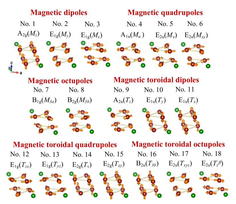
Figure 5: Symmetrized magnetic structures generated on Mn₃Sn crystal by cluster multipole method with each finite magnetic moment normalized to unity [17].

Several potential approaches can be considered for applying this method to crystals comprising various atom species. Here, we will take the simplest approach and treat only the magnetic atoms of interest, the Mn atoms, and ignore the other atoms, implying that the presence of nonmagnetic atoms affects the formation of the magnetic structure even though it is not treated explicitly. This method makes it possible to compare the crystals composed of different crystal structures and atomic species as demonstrated by comparing the magnetic structures of Mn₃Ir and Mn₃Sn later.

Figures 6 and 7 show the correlation tables of the normalized similarity kernels $\overline{K}^{(2)}$, $K^{(2)}$, $\overline{K}^{(4)}$, and $K^{(4)}$ calculated for the symmetrized magnetic structures of Fig. 4 and 5, respectively. The similarity kernels $K^{(\xi)}$ ($\xi=2,4$) show better resolution to distinguish the different magnetic structures than those designed to neglect the magnetic anisotropy, $\overline{K}^{(\xi)}$, for the same $\xi$, and the fourth-order similarity kernels show better resolution than the second-order ones. Thus, $\overline{K}^{(2)}$ has the least ability to distinguish the magnetic structure, while $K^{(4)}$ demonstrates the maximum capability to distinguish the different magnetic structures, as discussed in detail below.

The magnetic dipole structures of No. 1-3 in Figs. 4 and 5 are ordinary ferromagnetic structures along different axes and differ only in magnetic anisotropy. In Fig. 4, since the magnetic structures No. 5 and No. 6 are obtained by 90 degrees of spin rotation on each atom of No. 8 and No. 9, respectively, those two magnetic structures differ only in magnetic anisotropy. Similarly, in Fig. 5, the magnetic structures of No. 5 and No. 7 differ from No. 6 and No. 8, respectively, in magnetic anisotropy. As a result, the $\overline{K}^{(\xi)}$ evaluate that they are equivalent for those magnetic structures irrespective of the order $\xi$, as shown in Figs. 6 and 7 for $\xi$=2, 4. In addition, $\overline{K}^{(2)}$ and $\overline{K}^{(4)}$ barely reflect the magnetic structural differences that go beyond the magnetic anisotropy, such as No. 5 and 6 in Fig. 4 and No. 4 and 5 in Fig. 5, by showing the value close to 1.0. $K^{(2)}$ shows moderate discrimination performance for magnetic structures with different magnetic symmetries and succeeds in finding differences in magnetic anisotropy, but it still fails to discriminate several magnetic structures that involve differences in magnetic anisotropy. $K^{(4)}$ shows significantly better discrimination performance for magnetic structures distinct from both magnetic symmetry and magnetic anisotropy. However, even with the $K^{(4)}$, it is hard to distinguish the difference in the hexagonal in-plane magnetic anisotropy between No.2 and 3 and between No.17 and 18, as discussed in Sec. III.1, suggesting a partial spectrum of the order higher than four is required to distinguish the difference of the hexagonal in-plane magnetic anisotropy.

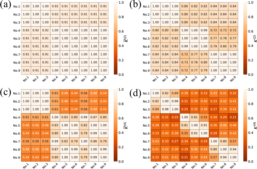
Figure 6: Pair plots of normalized similarity kernels of the power spectrum and trispectrum with $\sigma$=4.0Å, $n_{\rm max}$=4, ${\color[rgb]{0,0,0}\ell}_{\rm max}$=6, and $r_{\rm cut}$=5Å for the magnetic structures corresponding to Fig. 4 for (a) $\overline{K}^{(2)}$, (b) $K^{(2)}$, (c) $\overline{K}^{(4)}$, and (d) $K^{(4)}$.

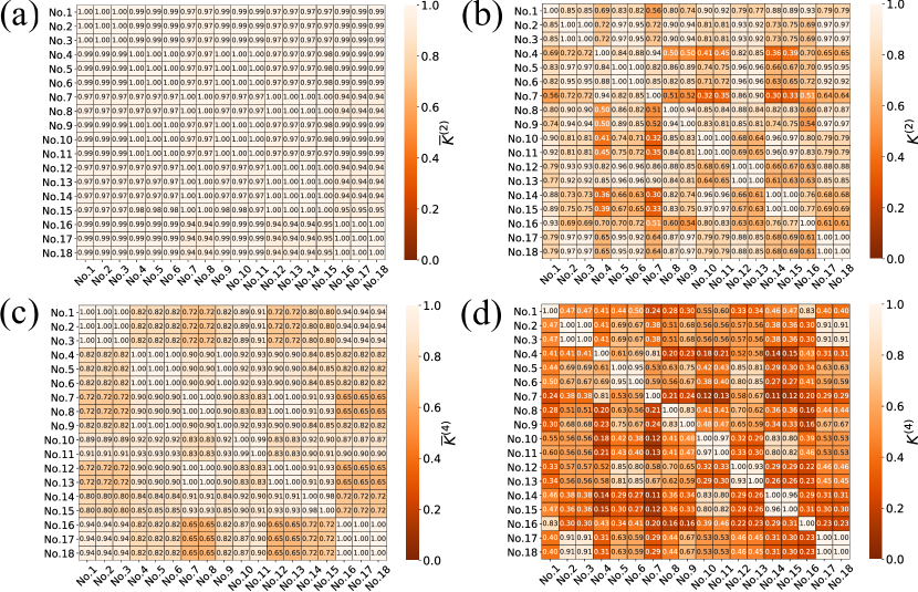
Figure 7: Pair plots of normalized similarity kernels of the power spectrum and trispectrum with $\sigma$=4.0Å, $n_{\rm max}$=4, ${\color[rgb]{0,0,0}\ell}_{\rm max}$=6, and $r_{\rm cut}$=5Å for magnetic structures corresponding to Fig. 5 for (a) $\overline{K}^{(2)}$, (b) $K^{(2)}$, (c) $\overline{K}^{(4)}$, and (d) $K^{(4)}$.

As mentioned above, the similarity of the local magnetic environment can be evaluated for different magnetic compounds with different crystal structures by focusing on specific magnetic ions that both compounds contain. Figure 8 provides the correlation table between the magnetic structures of Mn₃Ir in Fig. 4 and those of Mn₃Sn in Fig. 5, using $\sigma$=1.0Å and $\sigma$=4.0Å with $n_{\rm max}$=4, ${\color[rgb]{0,0,0}\ell}_{\rm max}$=6, and $r_{\rm cut}$=5.0Å. For $\sigma$=1.0Å, the width of the magnetization density around each Mn atom is small, and there is little overlap between the magnetization densities coming from different magnetic atoms, resulting in the dominant contribution of Eq. (11) for the trispectrum, Eqs. (34) and (23). In this case, the difference in the magnetic structures is reflected only through the averaging procedure of the origin choice in Eq. (34), and the ferromagnetic structures can not be distinguished even for the different crystals. In Fig. 8, No. 4 of Mn₃Ir and No. 15 of Mn₃Sn are evaluated as closer to ferromagnetism than the others. This reflects that these magnetic structures have finite magnetizations in their ferrimagnetic structure. The magnetization densities broadened with a value of $\sigma$=4.0Å lead to significant overlap between the magnetization densities from different magnetic atoms. This causes the difference in the partial spectra for the distinct magnetic environments around the Mn atoms in Mn₃Ir and Mn₃Sn, increasing discrimination performance for both compounds even in the case of ferromagnetic structures, as depicted in Fig. 8 (b).

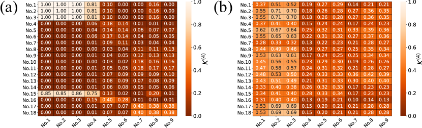
Figure 8: Pair plots of normalized similarity kernel $K^{(4)}$ between the symmetrized magnetic structures of Mn₃Ir and of Mn₃Sn, shown in Fig. 4 and Fig. 5. The calculations use $n_{\rm max}$=4, ${\color[rgb]{0,0,0}\ell}_{\rm max}$=6, and $r_{\rm cut}$=5Å with (a) $\sigma$=1.0Å and (b) $\sigma$=4.0Å.

IV Summary

We have developed a theory of descriptors for magnetic structures invariant to arbitrary choices of the coordinate axis, crystal unit cells, and origin choices. Higher-order partial spectra are essential to discriminate different magnetic structures that share the same atomic positions, especially with differences in magnetic anisotropy. We have also derived the fourth-order partial spectrum, referred to as the trispectrum, and compared its properties to the second-order partial spectrum, i.e., the power spectrum. The trispectrum effectively distinguishes magnetic structures only with magnetic anisotropy difference, though the power spectrum cannot discriminate them. Therefore, the trispectrum is necessary to accurately classify magnetic symmetries relevant to the physical properties of magnetic materials. Additionally, we have derived alternative partial spectra irrelevant to magnetic anisotropy and confirmed their effectiveness. These modified partial spectra are particularly useful for classifying magnetic structures obtained from first-principles calculations without spin-orbit coupling. Our theory of descriptors for magnetic structures thus provides a powerful tool for accurately classifying magnetic structures and paves the way for new applications in materials science and engineering by machine learning.

Supplementary information

The crystal of Mn₃Ir belongs to the space group $Pm\overline{3}m$ ($O_{h}^{1}$, No.221) and has three Mn atoms on the $3c$ Wycoff site [Mn1:(0,$\frac{1}{2}$,$\frac{1}{2}$), Mn2: ($\frac{1}{2}$,0,$\frac{1}{2}$), Mn3: ($\frac{1}{2}$,$\frac{1}{2}$,0)] and one Ir atom on the $1a$ site at (0,0,0) in the unit cell. Mn₃Sn belongs to the space group $P6_{3}/mmc$ ($D_{6h}^{4}$, No.194) and has six Mn atoms on $6h$ site [Mn1:($x$,2$x$,$\frac{1}{4}$), Mn2:($\overline{x}$,$x$,$\frac{3}{4}$), Mn3:($\overline{x}$,2$\overline{x}$,$\frac{3}{4}$), Mn4:($x$,$\overline{x}$,$\frac{1}{4}$), Mn5:(2$\overline{x}$,$\overline{x}$,$\frac{1}{4}$),Mn6:(2$x$,$x$,$\frac{3}{4}$) with $x$=0.8388] and Sn atoms on $2d$ site [Sn1:($\frac{1}{3}$, $\frac{2}{3}$, $\frac{3}{4}$), Sn2:($\frac{2}{3}$,$\frac{1}{3}$,$\frac{1}{4}$)]. Magnetic moment at each Mn site of Mn₃Ir and Mn₃Sn are provided in Tabs. S2 and S2.

Table S1: List of symmetrized magnetic structures in Mn₃Ir.

No. 1	Mn1:( 1.000000, 0.000000, 0.000000)	Mn2:( 1.000000, 0.000000, 0.000000)	Mn3:( 1.000000, 0.000000, 0.000000)
No. 2	Mn1:( 0.707107, 0.707107, 0.000000)	Mn2:( 0.707107, 0.707107, 0.000000)	Mn3:( 0.707107, 0.707107, 0.000000)
No. 3	Mn1:( 0.577350, 0.577350, 0.577350)	Mn2:( 0.577350, 0.577350, 0.577350)	Mn3:( 0.577350, 0.577350, 0.577350)
No. 4	Mn1:(-1.000000, 0.000000, 0.000000)	Mn2:( 1.000000, 0.000000, 0.000000)	Mn3:( 1.000000, 0.000000, 0.000000)
No. 5	Mn1:(-0.894427, 0.447214, 0.000000)	Mn2:( 0.447214,-0.894427, 0.000000)	Mn3:( 0.707107, 0.707107, 0.000000)
No. 6	Mn1:(-0.816497, 0.408248, 0.408248)	Mn2:( 0.408248,-0.816497, 0.408248)	Mn3:( 0.408248, 0.408248,-0.816497)
No. 7	Mn1:( 0.000000, 0.000000, 0.000000)	Mn2:(-1.000000, 0.000000, 0.000000)	Mn3:( 1.000000, 0.000000, 0.000000)
Mo. 8	Mn1:( 0.000000, 1.000000, 0.000000)	Mn2:(-1.000000, 0.000000, 0.000000)	Mn3:( 0.707107,-0.707107, 0.000000)
No. 9	Mn1:( 0.000000, 0.707107,-0.707107)	Mn2:(-0.707107, 0.000000, 0.707107)	Mn3:( 0.707107,-0.707107, 0.000000)

Table S2: List of symmetrized magnetic structures in Mn₃Sn.

No. 1	Mn1:( 0.000000 0.000000 1.000000)	Mn2:( 0.000000 0.000000 1.000000)	Mn3:( 0.000000 0.000000 1.000000)
	Mn4:( 0.000000 0.000000 1.000000)	Mn5:( 0.000000 0.000000 1.000000)	Mn6:( 0.000000 0.000000 1.000000)
No. 2	Mn1:( 0.000000,-1.000000, 0.000000)	Mn2:( 0.000000,-1.000000, 0.000000)	Mn3:( 0.000000,-1.000000, 0.000000)
	Mn4:( 0.000000,-1.000000, 0.000000)	Mn5:( 0.000000,-1.000000, 0.000000)	Mn6:( 0.000000,-1.000000, 0.000000)
No. 3	Mn1:( 1.000000, 0.000000, 0.000000)	Mn2:( 1.000000, 0.000000, 0.000000)	Mn3:( 1.000000, 0.000000, 0.000000)
	Mn4:( 1.000000, 0.000000, 0.000000)	Mn5:( 1.000000, 0.000000, 0.000000)	Mn6:( 1.000000, 0.000000, 0.000000)
No. 4	Mn1:( 0.000000,-1.000000, 0.000000)	Mn2:( 0.866025,-0.500000, 0.000000)	Mn3:( 0.000000, 1.000000, 0.000000)
	Mn4:(-0.866025, 0.500000, 0.000000)	Mn5:( 0.866025, 0.500000, 0.000000)	Mn6:(-0.866025,-0.500000, 0.000000)
No. 5	Mn1:( 0.000000,-1.000000, 0.000000)	Mn2:(-0.866025,-0.500000, 0.000000)	Mn3:( 0.000000, 1.000000, 0.000000)
	Mn4:( 0.866025, 0.500000, 0.000000)	Mn5:(-0.866025, 0.500000, 0.000000)	Mn6:( 0.866025,-0.500000, 0.000000)
No. 6	Mn1:( 1.000000, 0.000000, 0.000000)	Mn2:( 0.500000,-0.866025, 0.000000)	Mn3:(-1.000000, 0.000000, 0.000000)
	Mn4:(-0.500000, 0.866025, 0.000000)	Mn5:(-0.500000,-0.866025, 0.000000)	Mn6:( 0.500000, 0.866025, 0.000000)
No. 7	Mn1:( 0.000000, 1.000000, 0.000000)	Mn2:( 0.866025,-0.500000, 0.000000)	Mn3:( 0.000000, 1.000000, 0.000000)
	Mn4:( 0.866025,-0.500000, 0.000000)	Mn5:(-0.866025,-0.500000, 0.000000)	Mn6:(-0.866025,-0.500000, 0.000000)
Mo. 8	Mn1:(-1.000000, 0.000000, 0.000000)	Mn2:( 0.500000, 0.866025, 0.000000)	Mn3:(-1.000000, 0.000000, 0.000000)
	Mn4:( 0.500000, 0.866025, 0.000000)	Mn5:( 0.500000,-0.866025, 0.000000)	Mn6:( 0.500000,-0.866025, 0.000000)
No. 9	Mn1:(-1.000000, 0.000000, 0.000000)	Mn2:(-0.500000,-0.866025, 0.000000)	Mn3:( 1.000000, 0.000000, 0.000000)
	Mn4:( 0.500000, 0.866025, 0.000000)	Mn5:( 0.500000,-0.866025, 0.000000)	Mn6:(-0.500000, 0.866025, 0.000000)
No.10	Mn1:( 0.000000, 0.000000, 0.000000)	Mn2:( 0.000000, 0.000000,-1.000000)	Mn3:( 0.000000, 0.000000, 0.000000)
	Mn4:( 0.000000, 0.000000, 1.000000)	Mn5:( 0.000000, 0.000000,-1.000000)	Mn6:( 0.000000, 0.000000, 1.000000)
No.11	Mn1:( 0.000000, 0.000000,-1.000000)	Mn2:( 0.000000, 0.000000,-1.000000)	Mn3:( 0.000000, 0.000000, 1.000000)
	Mn4:( 0.000000, 0.000000, 1.000000)	Mn5:( 0.000000, 0.000000, 1.000000)	Mn6:( 0.000000, 0.000000,-1.000000)
No.12	Mn1:( 0.000000,-1.000000, 0.000000)	Mn2:( 0.866025, 0.500000, 0.000000)	Mn3:( 0.000000,-1.000000, 0.000000)
	Mn4:( 0.866025, 0.500000, 0.000000)	Mn5:(-0.866025, 0.500000, 0.000000)	Mn6:(-0.866025, 0.500000, 0.000000)
No.13	Mn1:(-1.000000, 0.000000, 0.000000)	Mn2:( 0.500000,-0.866025, 0.000000)	Mn3:(-1.000000, 0.000000, 0.000000)
	Mn4:( 0.500000,-0.866025, 0.000000)	Mn5:( 0.500000, 0.866025, 0.000000)	Mn6:( 0.500000, 0.866025, 0.000000)
No.14	Mn1:( 0.000000, 0.000000, 0.000000)	Mn2:( 0.000000, 0.000000,-1.000000)	Mn3:( 0.000000, 0.000000, 0.000000)
	Mn4:( 0.000000, 0.000000,-1.000000)	Mn5:( 0.000000, 0.000000, 1.000000)	Mn6:( 0.000000, 0.000000, 1.000000)
No.15	Mn1:( 0.000000, 0.000000, 1.000000)	Mn2:( 0.000000, 0.000000,-1.000000)	Mn3:( 0.000000, 0.000000, 1.000000)
	Mn4:( 0.000000, 0.000000,-1.000000)	Mn5:( 0.000000, 0.000000,-1.000000)	Mn6:( 0.000000, 0.000000,-1.000000)
No.16	Mn1:( 0.000000, 0.000000, 1.000000)	Mn2:( 0.000000, 0.000000,-1.000000)	Mn3:( 0.000000, 0.000000,-1.000000)
	Mn4:( 0.000000, 0.000000, 1.000000)	Mn5:( 0.000000, 0.000000, 1.000000)	Mn6:( 0.000000, 0.000000,-1.000000)
No.17	Mn1:( 0.000000, 1.000000, 0.000000)	Mn2:( 0.000000,-1.000000, 0.000000)	Mn3:( 0.000000,-1.000000, 0.000000)
	Mn4:( 0.000000, 1.000000, 0.000000)	Mn5:( 0.000000, 1.000000, 0.000000)	Mn6:( 0.000000,-1.000000, 0.000000)
No.18	Mn1:(-1.000000, 0.000000, 0.000000)	Mn2:( 1.000000, 0.000000, 0.000000)	Mn3:( 1.000000, 0.000000, 0.000000)
	Mn4:(-1.000000, 0.000000, 0.000000)	Mn5:(-1.000000, 0.000000, 0.000000)	Mn6:( 1.000000, 0.000000, 0.000000)

References

- Behler and Parrinello [2007] J. Behler and M. Parrinello, Phys. Rev. Lett. 98, 146401 (2007).
- Bartók et al. [2010] A. P. Bartók, M. C. Payne, R. Kondor, and G. Csányi, Phy. Rev. Lett. 104, 136403 (2010).
- Behler [2011] J. Behler, J. Chem. Phys. 134, 074106 (2011).
- Rupp et al. [2012] M. Rupp, A. Tkatchenko, K. R. Müller, and O. A. von Lilienfeld, Physical Review Letters 108, 058301 (2012).
- Bartók et al. [2013] A. P. Bartók, R. Kondor, and G. Csányi, Phys. Rev. B 87, 184115 (2013).
- Faber et al. [2015] F. Faber, A. Lindmaa, O. A. von Lilienfeld, and R. Armiento, Int. J. Quantum Chem. 115, 1094 (2015).
- Glielmo et al. [2017] A. Glielmo, P. Sollich, and A. De Vita, Phys. Rev. B 95, 214302 (2017).
- Huo and Rupp [2022] H. Huo and M. Rupp, Mach. Learn.: Sci. Technol. 3, 045017 (2022).
- Bartók et al. [2018] A. P. Bartók, J. Kermode, N. Bernstein, and G. Csányi, Phys. Rev. X 8, 041048 (2018).
- Fujii et al. [2020] S. Fujii, T. Yokoi, C. A. Fisher, H. Moriwake, and M. Yoshiya, Nat. Commun. 11, 1854 (2020).
- Eckhoff and Behler [2021] M. Eckhoff and J. Behler, npj Comput Mater 7, 170 (2021).
- Novikov et al. [2022] I. Novikov, B. Grabowski, F. Körmann, and A. Shapeev, npj Comput. Mater. 8, 13 (2022).
- Domina et al. [2022] M. Domina, M. Cobelli, and S. Sanvito, 105, 214439 (2022).
- Varshalovich [1988] D. A. Varshalovich, Quantum Theory Of Angular Momemtum (World Scientific Pub Co Inc, 1988).
- Himanen et al. [2020] L. Himanen, M. O. J. Jäger, E. V. Morooka, F. F. Canova, Y. S. Ranawat, D. Z. Gao, P. Rinke, and A. S. Foster, Comp. Phys. Commun. 247, 106949 (2020).
- Collis et al. [1998] W. B. Collis, P. R. White, and J. K. Hammond, Mech. Syst. Signal Process. 12, 375 (1998).
- Suzuki et al. [2019] M.-T. Suzuki, T. Nomoto, R. Arita, Y. Yanagi, S. Hayami, and H. Kusunose, Phys. Rev. B 99, 174407 (2019).
- Huyen et al. [2019] V. T. N. Huyen, M.-T. Suzuki, K. Yamauchi, and T. Oguchi, Phys. Rev. B 100, 094426 (2019).