Systematic construction of topological-nontopological hybrid universal quantum gates
based on many-body Majorana fermion interactions

Abstract

Topological quantum computation by way of braiding of Majorana fermions is not universal quantum computation. There are several attempts to make universal quantum computation by introducing some additional quantum gates or quantum states. However, there is an embedding problem that $M$-qubit gates cannot be embedded straightforwardly in $N$ qubits for $N>M$. This problem is inherent to the Majorana system, where logical qubits are different from physical qubits because braiding operations preserve the fermion parity. By introducing $2N$-body interactions of Majorana fermions, topological-nontopological hybrid universal quantum computation is shown to be possible. Especially, we make a systematic construction of the CⁿZ gate, CⁿNOT gate and the CⁿSWAP gate.

A quantum computer is a promising next generation computer[1, 2, 3]. In order to execute any quantum algorithms, universal quantum computation is necessary[4, 5, 6]. There are various approaches to realize universal computation including superconductors[7], photonic systems[8], quantum dots[9], trapped ions[10] and nuclear magnetic resonance[11, 12]. The Solovay-Kitaev theorem dictates that only the Hadamard gate, the $\pi/4$ phase-shift gate and the CNOT gate are enough for universal quantum computation. These one and two-qubit quantum gates can be embedded to larger qubits straightforwardly in these approaches.

Braiding of Majorana fermions is the most promising method for topological quantum computation[13, 14, 15, 16, 17]. There are various approaches to materialize Majorana fermions such as fractional quantum Hall effects[18, 19, 16, 20], topological superconductors[21, 22, 23, 24, 25, 26, 27] and Kitaev spin liquids[28, 29]. However, it can generate only a part of Clifford gate[30, 31]. The entire Clifford gates are generated for two qubits but not for more than three qubits[31]. Furthermore, only the Clifford gates are not enough to exceed classical computers, which is known as the Gottesman-Knill theorem[32, 33, 34].

There are several attempts to make universal quantum computation based on Majorana fermions[30, 20, 35, 36, 24, 37, 38, 39, 40, 41]. In the Majorana system, it is necessary to construct logical qubits from physical qubits by taking a parity definite basis, because braiding preserves the fermion parity. It makes logical qubits nonlocal. It is a nontrivial problem to embed a nonlocal $M$-qubit quantum gate in the $N$-qubit system with $N>M$. Hence, even if the Hadamard gate, the $\pi/4$ phase-shift gate and the CNOT gate are constructed, it is not enough for universal quantum computation in the $N$-qubit system unless this embedding problem is resolved.

In this paper, we systematically construct various quantum gates for universal quantum computation by introducing $2N$-body interactions of Majorana fermions preserving the fermion parity. We have required the fermion parity preservation because it is beneficial to use the standard braiding process as much as possible due to its topological protection. By combining topological quantum gates generated by braiding and additional quantum gates generated by many-body interactions of Majorana fermions, topological-nontopological hybrid universal quantum computation is possible. It would be more robust than conventional universal quantum computation because the quantum gates generated by braiding are topologically protected. We systematically construct arbitrary Cⁿ-phase shift gates, the Hadamard gate, CⁿNOT gates and CⁿSWAP gates in the $N$-qubit system by this generalization.

Supplementary Materials are prepared for detailed analysis in the case of small qubits to make clear a general analysis for the $N$-qubit system.

Physical qubits and logical qubits: Majorana fermions are described by operators $\gamma_{\alpha}$ satisfying the anticommutation relations

$$\left\{\gamma_{\alpha},\gamma_{\beta}\right\}=2\delta_{\alpha\beta}.$$ (1)

The braid operator is defined by[14]

$$\mathcal{B}_{\alpha\beta}=\exp\left[\frac{\pi}{4}\gamma_{\beta}\gamma_{\alpha}\right]=\frac{1}{\sqrt{2}}\left(1+\gamma_{\beta}\gamma_{\alpha}\right).$$ (2)

It satisfies $\mathcal{B}_{\alpha\beta}^{4}=1$ and there is a corresponding anti-braiding operator $\mathcal{B}_{\alpha\beta}^{-1}=\mathcal{B}_{\alpha\beta}^{3}$.

The qubit basis is defined by[14]

$$\left|n_{N+1}n_{N}\cdots n_{2}n_{1}\right\rangle_{\text{physical}}$$ (3)

$$\equiv \left(c_{1}^{\dagger}\right)^{n_{1}}\left(c_{2}^{\dagger}\right)^{n_{2}}\cdots\left(c_{N}^{\dagger}\right)^{n_{N}}\left(c_{N+1}^{\dagger}\right)^{n_{N+1}}\left|0\right\rangle,$$

with $n_{\alpha}=0$ or $1$, where ordinary fermion operators are constructed from two Majorana fermions as

$$c_{\alpha}=\frac{1}{2}\left(\gamma_{2\alpha-1}+i\gamma_{2\alpha}\right).$$ (4)

$2N+4$ Majorana fermions constitute $N+1$ physical qubits.

The braiding operation preserves the fermion parity $P_{\alpha\beta}\equiv i\gamma_{\beta}\gamma_{\alpha}$, where it commutes with the braid operator $\mathcal{B}_{\alpha\beta}$,

$$\left[\mathcal{B}_{\alpha\beta},P_{\alpha\beta}\right]=0.$$ (5)

It means that if we start with the even parity state $\left|00\cdots 0\right\rangle_{\text{physical}}$, the states after any braiding process should have even fermion parity. Therefore, in order to construct $N$ logical qubits $\left|n_{N}\cdots n_{2}n_{1}\right\rangle_{\text{logical}}$, $N+1$ physical qubits $\left|n_{N+1}^{\prime}\cdots n_{2}^{\prime}n_{1}^{\prime}\right\rangle_{\text{physical}}$ are necessary[42, 43, 44]. There are $N!$ correspondences between the logical and physical qubits in general. However, we adopt the following unique correspondence. When the logical qubit $\left|n_{N}\cdots n_{2}n_{1}\right\rangle_{\text{logical}}$ is given, we associate to it a physical qubit $\left|n_{N}\cdots n_{2}n_{1}n_{0}\right\rangle_{\text{physical}}$ by adding one qubit $n_{0}$ uniquely so that $\sum_{\alpha=0}^{N}n_{\alpha}=0$ mod $2$. Alternatively, when a physical qubit $\left|n_{N}\cdots n_{2}n_{1}n_{0}\right\rangle_{\text{logical}}$ is given, we associate to it a logical qubit $\left|n_{N}\cdots n_{2}n_{1}\right\rangle_{\text{physical}}$ just by eliminating the qubit $n_{0}$. An example reads as follows,

$$\left(\overbrace{\begin{array}[]{c}\left|0,\cdots,0,0,0\right\rangle\\ \left|0,\cdots,0,0,1\right\rangle\\ \left|0,\cdots,0,1,0\right\rangle\\ \left|0,\cdots,0,1,1\right\rangle\\ \left|0,\cdots,1,0,0\right\rangle\\ \left|0,\cdots,1,0,1\right\rangle\\ \cdots\end{array}}^{N}\right)_{\text{logical}}=\left(\overbrace{\begin{array}[]{c}\left|0,\cdots,0,0,0,0\right\rangle\\ \left|0,\cdots,0,0,1,1\right\rangle\\ \left|0,\cdots,0,1,0,1\right\rangle\\ \left|0,\cdots,0,1,1,0\right\rangle\\ \left|0,\cdots,1,0,0,1\right\rangle\\ \left|0,\cdots,1,0,1,0\right\rangle\\ \cdots\end{array}}^{N+1}\right)_{\text{physical}}.$$ (6)

This correspondence is different from those in the previous works[13, 43, 44, 45, 46, 47]. Accordingly, the detailed braiding process for quantum gates are slightly different from the previous ones[43, 44, 45, 46, 47].

$2N$-body interactions: A generic operator involving two Majorana fermions $\gamma_{\alpha}$ and $\gamma_{\beta}$ is expressed as $U_{\alpha\beta}=a_{1}+a_{2}\gamma_{\alpha}+a_{3}\gamma_{\beta}+a_{4}\gamma_{\beta}\gamma_{\alpha}$, since higher-order terms $\gamma_{\alpha}^{p}\gamma_{\beta}^{q}$ are absent for $p\geq 2$ and $q\geq 2$ because of the relations $\gamma_{\alpha}^{2}=\gamma_{\beta}^{2}=1$. Then, by imposing the parity conservation condition $\left[U_{\alpha\beta},P_{\alpha\beta}\right]=0$ with the fermion-parity operator $P_{\alpha\beta}=\gamma_{\beta}\gamma\alpha$, it is restricted to $U_{\alpha\beta}=a_{1}+a_{4}\gamma_{\beta}\gamma_{\alpha}$. Furthermore, the unitary condition $U_{\alpha\beta}U_{\alpha\beta}=U_{\alpha\beta}^{\dagger}U_{\alpha\beta}=1$ leads to the representation of $U_{\alpha\beta}$ in the form of

$$U_{\alpha\beta}\left(\theta\right) =\exp(\theta\gamma_{\beta}\gamma_{\alpha})=\cos\theta+\gamma_{\beta}\gamma_{\alpha}\sin\theta,$$ (7)

$$(U_{\alpha\beta}\left(\theta\right))^{-1} =\exp(-\theta\gamma_{\beta}\gamma_{\alpha})=\cos\theta-\gamma_{\beta}\gamma_{\alpha}\sin\theta.$$ (8)

The choice $\theta=\pi/4$ corresponds to the braiding operation. In general, $\theta$ can take an arbitrary value.

This operator transforms the Majorana operators as

$$U_{\alpha\beta}\left(\theta\right)\gamma_{\alpha}(U_{\alpha\beta}\left(\theta\right))^{-1} =\gamma_{\alpha}\cos 2\theta+\gamma_{\beta}\sin 2\theta,$$

$$U_{\alpha\beta}\left(\theta\right)\gamma_{\beta}(U_{\alpha\beta}\left(\theta\right))^{-1} =-\gamma_{\alpha}\sin 2\theta+\gamma_{\beta}\cos 2\theta.$$ (9)

We show that non-Clifford gates are constructed based on them.

The two-body operation is realized by the unitary dynamics,

$$\mathcal{B}_{\alpha\beta}\left(\theta\right)=\exp\left[\theta\gamma_{\beta}\gamma_{\alpha}\right]=\exp\left[iHt/\hbar\right],$$ (10)

with

$$H=\frac{\hbar\theta}{t}\gamma_{\beta}\gamma_{\alpha}.$$ (11)

The four-body operation

$$\mathcal{B}_{1234}^{(4)}\equiv\exp\left[i\frac{\pi}{4}\gamma_{4}\gamma_{3}\gamma_{2}\gamma_{1}\right]$$ (12)

is introduced[13] as an essential ingredient of universal quantum computation. We generalize it to the four-body operation $\mathcal{B}_{\alpha\beta\gamma\delta}^{\left(4\right)}\left(\theta\right)$ defined by

$$\mathcal{B}_{\alpha\beta\gamma\delta}^{(4)}\left(\theta\right) \equiv \exp\left[i\theta\gamma_{\delta}\gamma_{\gamma}\gamma_{\beta}\gamma_{\alpha}\right]$$ (13)

$$= \cos\theta+i\gamma_{\delta}\gamma_{\gamma}\gamma_{\beta}\gamma_{\alpha}\sin\theta,$$

which keeps the parity

$$\left[\mathcal{B}_{\alpha\beta\gamma\delta}^{\left(4\right)}\left(\theta\right),P_{\alpha\beta}\right]=0.$$ (14)

We use an abbreviation,

$$\mathcal{B}_{\alpha}^{\left(4\right)}\left(\theta\right)\equiv\mathcal{B}_{\alpha,\alpha+1.\alpha+2,\alpha+3}^{(4)}\left(\theta\right).$$ (15)

The relation

$$\left(\mathcal{B}_{1}^{\left(4\right)}\left(\theta\right)\right)^{\dagger}\mathcal{B}_{1}^{\left(4\right)}\left(\theta\right)=I$$ (16)

holds because of the coefficient $i$ in Eq.(13).

It is realized by the unitary dynamics,

$$\mathcal{B}_{\alpha\beta\gamma\delta}^{\left(4\right)}\left(\theta\right)=\exp\left[iHt/\hbar\right],$$ (17)

with

$$H=\frac{i\hbar\theta}{t}\gamma_{\delta}\gamma_{\gamma}\gamma_{\beta}\gamma_{\alpha}.$$ (18)

Similary, we may define the $2N$-body operation by

$$\mathcal{B}_{1}^{\left(2N\right)}\left(\theta\right) \equiv \mathcal{B}_{1\sim 2N}^{(2N)}\left(\theta\right)\equiv\exp\left[i^{(N-1)\theta}\gamma_{2N}\gamma_{2N-1}\cdots\gamma_{2}\gamma_{1}\right]$$ (19)

$$= \cos\theta+i^{N-1}\gamma_{2N}\gamma_{2N-1}\cdots\gamma_{2}\gamma_{1}\sin\theta.$$

It satisfies the unitary condition,

$$\left(\mathcal{B}_{1}^{\left(2N\right)}\left(\theta\right)\right)^{\dagger}\mathcal{B}_{1}^{\left(2N\right)}\left(\theta\right)=I.$$ (20)

We also define

$$\mathcal{B}_{\alpha}^{\left(2N\right)}\left(\theta\right)\equiv\mathcal{B}_{\alpha,\alpha+1.\cdots\alpha+2N-2,\alpha+2N-1}\left(\theta\right).$$ (21)

It is realized by the $2N$-body interaction of Majorana fermions

$$H=\frac{i^{N-1}\hbar\theta}{t}\gamma_{2N}\gamma_{2N-1}\cdots\gamma_{2}\gamma_{1}.$$ (22)

$N$ physical qubits: We consider the $2N$ Majorana fermion system. The explicit actions on $2N$ physical qubits are given by

$$\mathcal{B}_{1}\left(\theta\right) = I_{2N-2}\otimes R_{z}\left(2\theta\right),$$

$$\mathcal{B}_{3}\left(\theta\right) = I_{2N-4}\otimes R_{z}\left(2\theta\right)\otimes I_{2},$$

$$\cdots$$

$$\mathcal{B}_{2n-1}\left(\theta\right) = I_{2N-2n}\otimes R_{z}\left(2\theta\right)\otimes I_{2n-2},$$

$$\cdots$$

$$\mathcal{B}_{2N-1}\left(\theta\right) = R_{z}\left(2\theta\right)\otimes I_{2N-2}$$ (23)

for odd numbers and

$$\mathcal{B}_{2}\left(\theta\right) =I_{2N-4}\otimes U_{xx}\left(\theta\right),$$

$$\cdots$$

$$\mathcal{B}_{2n}\left(\theta\right) =I_{2N-2-2n}\otimes U_{xx}\left(\theta\right)\otimes I_{2n-2},$$

$$\cdots$$

$$\mathcal{B}_{2N-2}\left(\theta\right) =U_{xx}\left(\theta\right)\otimes I_{2N-4}$$ (24)

for even numbers, where we have defined the rotation along the $z$ axis by

$$R_{z}\left(\theta\right)\equiv\exp\left[-i\frac{\theta}{2}\sigma_{z}\right]=\text{diag.}\left(e^{-i\theta/2},e^{i\theta/2}\right),$$ (25)

and

$$U_{xx}\left(\theta\right)\equiv\exp\left[-i\theta\sigma_{x}\otimes\sigma_{x}\right].$$ (26)

$N-1$ logical qubits: $N-1$ logical qubits are constructed from $N$ physical qubits based on the correspondence (6).

Local $z$ rotation is possible for any qubits as in

$$\mathcal{B}_{1}\left(\theta\right) = \exp\left[-i\theta\bigotimes_{j=1}^{N-1}\sigma_{z}\right],$$

$$\mathcal{B}_{3}\left(\theta\right) = I_{2N-4}\otimes R_{z}\left(2\theta\right)$$

$$= \exp\left[-i\theta I_{2}\otimes I_{2}\otimes\sigma_{z}\right],$$

$$\cdots$$

$$\mathcal{B}_{2n-1}\left(\theta\right) = I_{2N-2n}\otimes R_{z}\left(2\theta\right)\otimes I_{2n-4}$$

$$= \exp\left[-i\theta I_{2N-2n}\otimes\sigma_{z}\otimes I_{2n-4}\right],$$

$$\cdots$$

$$\mathcal{B}_{2N-3}\left(\theta\right) = I_{2}\otimes R_{z}\left(2\theta\right)\otimes I_{2N-2n-6}$$ (27)

$$= \exp\left[-i\theta I_{2}\otimes\sigma_{z}\otimes I_{2N-2n-6}\right].$$

Local $x$ rotation is possible for any qubits as in

$$\mathcal{B}_{23}\left(\theta\right) = I_{2N-4}\otimes R_{x}\left(2\theta\right),$$

$$\mathcal{B}_{2\sim 5}^{\left(4\right)}\left(\theta\right) = I_{2N-6}\otimes R_{x}\left(2\theta\right)\otimes I_{2},$$

$$\mathcal{B}_{2\sim 7}^{\left(6\right)}\left(\theta\right) = I_{2N-8}\otimes R_{x}\left(2\theta\right)\otimes I_{4},$$

$$\cdots$$

$$\mathcal{B}_{2\sim 2N-3}^{\left(2N-4\right)}\left(\theta\right) = I_{2}\otimes R_{x}\left(2\theta\right)\otimes I_{2N-6},$$

$$\mathcal{B}_{2\sim 2N-1}^{\left(2N-2\right)}\left(\theta\right) = R_{x}\left(2\theta\right)\otimes I_{2N-4},$$ (28)

where we have defined the rotation along the $x$ axis by

$$R_{x}\left(\theta\right)\equiv\exp\left[-i\frac{\theta}{2}\sigma_{x}\right]=\left(\begin{array}[]{cc}\cos\frac{\theta}{2}&-i\sin\frac{\theta}{2}\\ -i\sin\frac{\theta}{2}&\cos\frac{\theta}{2}\end{array}\right),$$ (29)

and $\mathcal{B}_{\alpha\sim\beta}\left(\theta\right)\equiv\mathcal{B}_{\alpha,\alpha+1,\cdots\beta-1,\beta}\left(\theta\right)$. Accordingly, the Hadamard gate is embedded in arbitrary $N$ qubits by using the decomposition formula,

$$U_{\text{H}}=R_{z}\left(\frac{\pi}{4}\right)R_{x}\left(\frac{\pi}{4}\right)R_{z}\left(\frac{\pi}{4}\right).$$ (30)

Next, we show that it is possible to construct any $2^{N}$ diagonal operators based on many-body Majorana interactions, and hence, an arbitrary Cⁿ-phase-shift gate is constructed. By applying the Hadamard gate, it is possible to construct the CⁿNOT gate. There are ${}_{N}C_{M}$ patterns of $2M$-body unitary evolutions in $2N$ physical qubits. By taking a sum, we have $\sum_{M=1N}^{N}C_{M}=2^{N}$ independent physical qubits. They produce $2^{N-1}$ independent logical qubits because there are complementary operators $\mathcal{B}_{\alpha}\left(\theta\right)$ and $\mathcal{B}_{\overline{\alpha}}\left(\theta\right)$ which produce the same logical qubits. The complementary operators are denoted as

$$\mathcal{B}_{\overline{\alpha}}\left(\theta\right)\simeq\mathcal{B}_{\alpha}\left(\theta\right),$$ (31)

where $\overline{\alpha}$ indicates a set of indices which is the complementary set of $\alpha$ in the indices $1\sim 2N$. For example, we consider the case for four qubits $N=4$, where eight Majorana fermions exists. The following different braiding operators $\mathcal{B}_{56}$ and $\mathcal{B}_{123478}$ give an identical logical quantum gate

$$\mathcal{B}_{123478}\simeq\mathcal{B}_{56},$$ (32)

where $\alpha=56$ and $\overline{\alpha}=123478$ with $N=4$. See the full list of the complementary braiding operators for four physical qubits in Eq.(S143) in Supplementary Material.

There are $2^{N-1}$ independent components in $N-1$ logical qubits. On the other hand, there are $2^{N-1}$ independent many-body Majorana operators. Hence, it is possible to construct arbitrary diagonal operators by solving the linear equation. They include the Cⁿ-phase shift gates. Using the relation

$$U_{\text{C}^{n}\phi}=e^{\frac{i\phi}{2^{n+1}}}\prod_{q=1}^{{2}^{n+1}-1}\exp\left[\frac{\left(-1\right)^{\text{Mod}_{2}\sum_{p=1}^{n+1}p_{n}}}{2^{n+1}}\bigotimes_{p=1}^{n+1}\left(\sigma_{z}\right)^{q_{p}}\right]$$ (33)

with $q_{p}=0,1$, the Cⁿ-phase shift gate is constructed as

$$U_{\text{C}^{n}\phi}=e^{\frac{i\phi}{2^{n+1}}}\prod_{q=1}^{{2}^{n}}\mathcal{B}_{\text{odd},q}\left(\frac{\phi}{2^{n+1}}\right)\prod_{r=1}^{{2}^{n}-1}\mathcal{B}_{\text{even},r}\left(-\frac{\phi}{2^{n+1}}\right),$$ (34)

where $\mathcal{B}_{\text{odd}}$ contains odd number of $\sigma_{z}$ operators for logical qubits, while $\mathcal{B}_{\text{even}}$ contains even number of $\sigma_{z}$ operators for logical qubits. By setting $\phi=\pi$, we obtain the CⁿZ gate.

For example, the CZ gate in three qubits are embedded as

$$U_{\text{CZ}}^{3\rightarrow 2} =U_{\text{CZ}}\otimes I_{2}=e^{i\pi/4}\mathcal{B}_{56}\left(\frac{\pi}{4}\right)\mathcal{B}_{78}\left(\frac{\pi}{4}\right)\mathcal{B}_{1234}^{\left(4\right)}\left(-\frac{\pi}{4}\right),$$

$$U_{\text{CZ}}^{3\rightarrow 1} =e^{i\pi/4}\mathcal{B}_{34}\left(\frac{\pi}{4}\right)\mathcal{B}_{78}\left(\frac{\pi}{4}\right)\mathcal{B}_{1256}^{\left(4\right)}\left(-\frac{\pi}{4}\right),$$

$$U_{\text{CZ}}^{2\rightarrow 1} =I_{2}\otimes U_{\text{CZ}}=e^{i\pi/4}\mathcal{B}_{34}\left(\frac{\pi}{4}\right)\mathcal{B}_{56}\left(\frac{\pi}{4}\right)\mathcal{B}_{1278}^{\left(4\right)}\left(-\frac{\pi}{4}\right),$$ (35)

where $U_{\text{CZ}}^{p\rightarrow q}$ indicates that the controlloed qubit is $p$ and the target qubit is $q$. The CC$\phi$ phase-shift gate acting on three logical qubits in given by

$$U_{\text{CC}\phi} = e^{i\phi/8}\mathcal{B}_{12}\left(\frac{\phi}{8}\right)\mathcal{B}_{34}\left(\frac{\phi}{8}\right)\mathcal{B}_{56}\left(\frac{\phi}{8}\right)\mathcal{B}_{78}\left(\frac{\phi}{8}\right)$$ (36)

$$\mathcal{B}_{1234}^{\left(4\right)}\left(-\frac{\phi}{8}\right)\mathcal{B}_{1278}^{\left(4\right)}\left(-\frac{\phi}{8}\right)\mathcal{B}_{1256}^{\left(4\right)}\left(-\frac{\phi}{8}\right).$$

Especially, the CCZ gate is constructed as follows,

$$U_{\text{CCZ}} = e^{i\pi/8}\mathcal{B}_{12}\left(\frac{\pi}{8}\right)\mathcal{B}_{34}\left(\frac{\pi}{8}\right)\mathcal{B}_{56}\left(\frac{\pi}{8}\right)\mathcal{B}_{78}\left(\frac{\pi}{8}\right)$$ (37)

$$\mathcal{B}_{1234}^{\left(4\right)}\left(-\frac{\pi}{8}\right)\mathcal{B}_{1256}^{\left(4\right)}\left(-\frac{\pi}{8}\right)\mathcal{B}_{1278}^{\left(4\right)}\left(-\frac{\pi}{8}\right).$$

The Toffoli gate is constructed by applying the Hadamard gate to the CCZ gate as in

$$U_{\text{Toffloi}}=\left(I_{4}\otimes U_{\text{H}}\right)U_{\text{CCZ}}\left(I_{4}\otimes U_{\text{H}}\right).$$ (38)

See Fig.1(a1). The Fredkin gate is constructed by sequential applications of three Toffoli gates as in

$$U_{\text{Fredkin}}=U_{\text{Toffoli}}^{\left(3,2\right)\rightarrow 1}U_{\text{Toffoli}}^{\left(3,1\right)\rightarrow 2}U_{\text{Toffoli}}^{\left(3,2\right)\rightarrow 1},$$ (39)

where $U_{\text{CZ}}^{\left(p,q\right)\rightarrow r}$ indicates that the controlloed qubits are $p$ and $q$ while the target qubit is $r$. See Fig.1(b1).

The CⁿNOT gate is constructed from CⁿZ gate as

$$U_{\text{C}^{n}\text{NOT}}=\left(I_{2n-2}\otimes U_{\text{H}}\right)U_{\text{C}^{n}\text{Z}}\left(I_{2n-2}\otimes U_{\text{H}}\right),$$ (40)

where the Hadamard gate is applied to $n$th qubit. See Fig.1(a2).

The CⁿSWAP gate is constructed from the CⁿZ gate as

$$U_{\text{C}^{n}\text{SWAP}}=U_{\text{C}^{n}\text{NOT}}^{\overline{1}\rightarrow 1}U_{\text{C}^{n}\text{NOT}}^{\overline{2}\rightarrow 2}U_{\text{C}^{n}\text{NOT}}^{\overline{1}\rightarrow 1},$$ (41)

where $U_{\text{C}^{n}\text{NOT}}^{\overline{p}\rightarrow p}$ indicates that the target qubit is $p$ and the others are controlled qubits, where $\overline{p}$ indicates the complementary qubits of the qubit $p$. See Fig.1(b2).

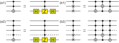
Figure 1: (a1) Construction of the CCNOT gate from the CCZ gate and the Hadamard gates. (a2) Construction of the CⁿNOT gate from the CⁿZ gate and the Hadamard gates. (b1) Construction of the Fredkin gate from three Toffoli gates. (b2) Construction of the CⁿSWAP gate from the CⁿNOT gates.

As a result, an arbitrary phase-shift gate, the CⁿNOT gate and the Hadamard gate are constructed in any logical qubits, and hence, the universal quantum computation is possible based on many-body interactions.

Discussions: We have analyzed the embedding problem inherent to the Majorana system, and shown that universal quantum computation is possible by introducing many-body interactions of Majorana fermions. Especially, the Cⁿ-phase shift gate, the CⁿNOT and the CⁿSWAP gate are systematically constructed, which are the basic ingredients of universal quantum computation based on the Solovay-Kitaev theorem. Although it was previously pointed out that four-body interactions of Majorana fermions are enough for universal quantum computation[13], we have shown that the four-body interactions are not enough but $2N$-body interactions are necessary.

The proposed quantum gates based on many-body interactions of Majorana fermions are not topologically protected because they are not generated by the standard braiding operations. By combining topological quantum computation based on braiding of Majorana fermions and nontopological quantum computation based on many-body interaction of Majorana fermions, topological-nontopological hybrid universal quantum computation is possible. It would be more robust than conventional universal quantum computation because many of quantum gates generated by braiding are topologically protected.

Recently, quantum simulation on Majorana fermions is studied in superconducting qubits[48, 49, 50]. It will be possible to realize many-body interactions of Majorana fermions in near future.

This work is supported by CREST, JST (Grants No. JPMJCR20T2) and Grants-in-Aid for Scientific Research from MEXT KAKENHI (Grant No. 23H00171).

I Results on conventional braiding

S1 Embedding

We consider a one-dimensional chain of Majorana fermions and only consider the braiding between adjacent Majorana fermions. We denote $\mathcal{B}_{\alpha}\equiv\mathcal{B}_{\alpha,\alpha+1}$. The braid operators $\mathcal{B}_{\alpha}$ satisfies the Artin braid group relation[1]

$$\mathcal{B}_{\alpha}\mathcal{B}_{\beta} =\mathcal{B}_{\beta}\mathcal{B}_{\alpha}\qquad\text{for\quad}\left|\alpha-\beta\right|\geq 2,$$

$$\mathcal{B}_{\alpha}\mathcal{B}_{\alpha+1}\mathcal{B}_{\alpha} =\mathcal{B}_{\alpha+1}\mathcal{B}_{\alpha}\mathcal{B}_{\alpha+1}.$$ (S1)

The embedding of an $M$-qubit quantum gate to an $N$-qubit system with $M<N$ is a nontrivial problem in braiding of Majorana fermions. There are two partial solutions. One is setting additional qubits to be $0$ as ancilla qubits, where every quantum gates can be embedded. The other is not to use the braiding $\mathcal{B}_{1}$. We discuss both of these in what follows.

S1.1 Ancilla embedding

$N-1$ logical qubits are embedded in $N$ logical qubits if the additional qubit is $0$,

$$\left|0n_{N-1}\cdots n_{2}n_{1}\right\rangle_{\text{logical}}.$$ (S2)

This is because the correspondence between the physical and logical qubits are identical if the $N$-th qubit is $0$. It is assured by the fact that we can use the same even parity basis in $(N-1)$ qubits because the $N$th qubit is $0$. On the other hand, the action is different if the additional qubit is $1$,

$$\left|1n_{N-1}\cdots n_{2}n_{1}\right\rangle_{\text{logical}}.$$ (S3)

This is because it is necessary to use the odd parity basis in physical $N-1$ qubits so that total parity is even in the presence of the $N$th qubit. It is still useful because there are many quantum algorithms where ancilla qubits are $0$.

S1.2 Braid construction

We study what $M$-qubit quantum gates can be embedded to an $N$-qubit quantum gate with $M<N$. First, we examine the case for one logical qubit as a simplest example. The braiding $\mathcal{B}_{1}$ acts differently on the even and odd bases,

$$\mathcal{B}_{1}^{\text{even}}\neq\mathcal{B}_{1}^{\text{odd}},$$ (S4)

where

$$\mathcal{B}_{1}^{\text{even}}=e^{-i\pi/4}\left(\begin{array}[]{cc}1&0\\ 0&i\end{array}\right),\qquad\mathcal{B}_{1}^{\text{odd}}=e^{-i\pi/4}\left(\begin{array}[]{cc}i&0\\ 0&1\end{array}\right).$$ (S5)

On the other hand, $\mathcal{B}_{2}$ and $\mathcal{B}_{3}$ act on even and odd bases in the same way,

$$\mathcal{B}_{2}^{\text{even}}=\mathcal{B}_{2}^{\text{odd}}=\frac{1}{\sqrt{2}}\left(\begin{array}[]{cc}1&-i\\ -i&1\end{array}\right),\qquad\mathcal{B}_{3}^{\text{even}}=\mathcal{B}_{3}^{\text{odd}}=e^{-i\pi/4}\left(\begin{array}[]{cc}1&0\\ 0&i\end{array}\right).$$ (S6)

Similarly, $\mathcal{B}_{k}$ for $k\geq 4$ has the same action on the even and odd bases. We find that embedding is possible if we do not use the braiding $\mathcal{B}_{1}$. Hence, all of the Pauli gates, the Hadamard transformation, the $i$SWAP gate can be embedded to the $N$-qubit quantum gates.

On the other hand, the quantum gates which use braiding $\mathcal{B}_{1}$ cannot be embedded to larger qubit as it is. For example, the CZ gate is given by the braiding $e^{-i\pi/4}\mathcal{B}_{5}^{-1}\left(\mathcal{B}_{3}\right)^{-1}\mathcal{B}_{1}$, whose matrix representation is

$$\text{diag.}\left(1,1,1,-1,i,-i,-i,-i\right),$$ (S7)

once it is embedded to three logical qubits. They are different,

$$e^{-i\pi/4}\mathcal{B}_{5}^{-1}\left(\mathcal{B}_{3}\right)^{-1}\mathcal{B}_{1}\neq I_{2}\otimes U_{\text{CZ}}=\text{diag.}\left(1,1,1,-1,1,1,1,-1\right),$$ (S8)

In general, $M$-quantum gates cannot be embedded in $N$ qubit. We solve the problem by introducing many-body interaction of Majorana fermions in Eq.(35).

S2 Single logical qubit

We discuss how to construct single logical qubit[2]. Two ordinary fermions $c_{1}$ and $c_{2}$ are introduced from four Majorana fermions as

$$c_{1}=\frac{1}{2}\left(\gamma_{1}+i\gamma_{2}\right),\qquad c_{2}=\frac{1}{2}\left(\gamma_{3}+i\gamma_{4}\right).$$ (S9)

The basis of physical qubits is given by

$$\Psi_{\text{physical}}=\left(\left|0\right\rangle,c_{1}^{\dagger}\left|0\right\rangle,c_{2}^{\dagger}\left|0\right\rangle,c_{1}^{\dagger}c_{2}^{\dagger}\left|0\right\rangle\right)^{t}\equiv\left(\left|0,0\right\rangle_{\text{physical}},\left|0,1\right\rangle_{\text{physical}},\left|1,0\right\rangle_{\text{physical}},\left|1,1\right\rangle_{\text{physical}}\right)^{t}.$$ (S10)

By taking the even parity basis as

$$\left(\begin{array}[]{c}\left|0\right\rangle\\ \left|1\right\rangle\end{array}\right)_{\text{logical}}=\left(\begin{array}[]{c}\left|0,0\right\rangle\\ \left|1,1\right\rangle\end{array}\right)_{\text{physical}},$$ (S11)

single logical qubit is constructed from two physical qubits.

S3 Quantum gates for one logical qubit

The braid operator $\mathcal{B}_{1}$ is written in terms of fermion operators,

$$\mathcal{B}_{1}=\frac{1}{\sqrt{2}}\left(1+\gamma_{2}\gamma_{1}\right)=\frac{1}{\sqrt{2}}\left(1+ic_{1}^{\dagger}c_{1}-ic_{1}c_{1}^{\dagger}\right),$$ (S12)

which operates on two physical qubits (S10) as[2]

$$\mathcal{B}_{1}\Psi_{\text{physical}}=e^{-i\pi/4}\left(\begin{array}[]{cccc}1&0&0&0\\ 0&i&0&0\\ 0&0&1&0\\ 0&0&0&i\end{array}\right)\left(\begin{array}[]{c}\left|0,0\right\rangle\\ \left|0,1\right\rangle\\ \left|1,0\right\rangle\\ \left|1,1\right\rangle\end{array}\right)_{\text{physical}}.$$ (S13)

Taking the even parity basis, the action is

$$\mathcal{B}_{1}\Psi_{\text{logical}}=e^{-i\pi/4}\left(\begin{array}[]{cc}1&0\\ 0&i\end{array}\right)\left(\begin{array}[]{c}\left|0\right\rangle\\ \left|1\right\rangle\end{array}\right)_{\text{logical}},$$ (S14)

where the basis for the logical qubit is defined by

$$\Psi_{\text{logical}}\equiv\left(\left|0\right\rangle,c_{1}^{\dagger}c_{2}^{\dagger}\left|0\right\rangle\right)^{t}.$$ (S15)

The braid operation is written as

$$\mathcal{B}_{1}=e^{-i\pi/4}U_{\text{S}},$$ (S16)

in terms of the S gate defined by

$$U_{\text{S}}\equiv\text{diag.}\left(1,i\right).$$ (S17)

The braid operator $\mathcal{B}_{2}$ is written in terms of fermion operators,

$$\mathcal{B}_{2}=\frac{1}{\sqrt{2}}\left(1+\gamma_{3}\gamma_{2}\right)=\frac{1}{\sqrt{2}}\left(1+ic_{2}c_{1}^{\dagger}+ic_{2}^{\dagger}c_{1}^{\dagger}-ic_{2}c_{1}-ic_{2}^{\dagger}c_{1}\right).$$ (S18)

It operates on two physical qubits (S10) as[2],

$$\mathcal{B}_{2}\Psi_{\text{physical}}=\frac{1}{\sqrt{2}}\left(\begin{array}[]{cccc}1&0&0&-i\\ 0&1&-i&0\\ 0&-i&1&0\\ -i&0&0&1\end{array}\right)\left(\begin{array}[]{c}\left|0,0\right\rangle\\ \left|0,1\right\rangle\\ \left|1,0\right\rangle\\ \left|1,1\right\rangle\end{array}\right)_{\text{physical}}=U_{xx}\left(\begin{array}[]{c}\left|0,0\right\rangle\\ \left|0,1\right\rangle\\ \left|1,0\right\rangle\\ \left|1,1\right\rangle\end{array}\right)_{\text{physical}},$$ (S19)

where

$$U_{xx}\equiv\frac{1}{\sqrt{2}}\left(\begin{array}[]{cccc}1&0&0&-i\\ 0&1&-i&0\\ 0&-i&1&0\\ -i&0&0&1\end{array}\right)=\exp\left[-i\frac{\pi}{4}\sigma_{x}\otimes\sigma_{x}\right].$$ (S20)

In the even parity basis, the action is

$$\mathcal{B}_{2}=\frac{1}{\sqrt{2}}\left(\begin{array}[]{cc}1&-i\\ -i&1\end{array}\right)=\exp\left[-i\frac{\pi}{4}\sigma_{x}\right]\equiv R_{x}.$$ (S21)

It has the relation

$$\mathcal{B}_{2}=e^{-i\pi/4}U_{\sqrt{\text{X}}},$$ (S22)

where $U_{\sqrt{\text{X}}}$ is the square-root of X gate defined by

$$U_{\sqrt{\text{X}}}\equiv\frac{1}{2}\left(\begin{array}[]{cc}1+i&1-i\\ 1-i&1+i\end{array}\right).$$ (S23)

The corresponding braiding is shown in Fig.S1(a).

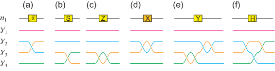
Figure S1: (a) Square-root of NOT gate, (b) S gate, (c) Pauli Z gate, (d) Pauli X gate, (e) Pauli Y gate and (f) Hadamard gate.

The braiding operator $\mathcal{B}_{3}$ is written in terms of fermion operators

$$\mathcal{B}_{3}=\frac{1}{\sqrt{2}}\left(1+\gamma_{4}\gamma_{3}\right)=\frac{1}{\sqrt{2}}\left(1+ic_{2}^{\dagger}c_{2}-ic_{2}c_{2}^{\dagger}\right),$$ (S24)

which operates on two physical qubits (S10) as[2]

$$\mathcal{B}_{3}\Psi_{\text{physical}}=e^{-i\pi/4}\left(\begin{array}[]{cccc}1&0&0&0\\ 0&1&0&0\\ 0&0&i&0\\ 0&0&0&i\end{array}\right)\left(\begin{array}[]{c}\left|0,0\right\rangle\\ \left|0,1\right\rangle\\ \left|1,0\right\rangle\\ \left|1,1\right\rangle\end{array}\right)_{\text{physical}}.$$ (S25)

In the even parity basis, the action is the same as (S16),

$$\mathcal{B}_{3}=e^{-i\pi/4}U_{\text{S}},$$ (S26)

where the S gate is defined by (S17). The corresponding braiding is shown in Fig.S1(b).

The Pauli Z gate is given by double braiding of $\mathcal{B}_{3}$,

$$U_{\text{Z}}\equiv\text{diag.}\left(1,-1\right)=U_{\text{S}}^{2}=i\mathcal{B}_{3}^{2}.$$ (S27)

The corresponding braiding is shown in Fig.S1(c).

The Pauli X gate (NOT gate) is given[3] by double braiding of $\mathcal{B}_{2}$,

$$U_{\text{X}}\equiv\left(\begin{array}[]{cc}0&1\\ 1&0\end{array}\right)=i\mathcal{B}_{2}^{2}.$$ (S28)

The corresponding braiding is shown in Fig.S1(d).

Then, the Pauli Y gate is given by sequential applications of $\mathcal{B}_{2}$ and $\mathcal{B}_{3}$,

$$U_{\text{Y}}\equiv\left(\begin{array}[]{cc}0&-i\\ i&0\end{array}\right)=iU_{\text{X}}U_{\text{Z}}=-\mathcal{B}_{2}^{2}\mathcal{B}_{3}^{2}.$$ (S29)

The corresponding braiding is shown in Fig.S1(e).

The Hadamard gate is defined by

$$U_{\text{H}}\equiv\frac{1}{\sqrt{2}}\left(\begin{array}[]{cc}1&1\\ 1&-1\end{array}\right).$$ (S30)

It is known to be generated by triple braids as[4, 5]

$$U_{\text{H}}=i\mathcal{B}_{2}\mathcal{B}_{3}\mathcal{B}_{2}.$$ (S31)

The corresponding braiding is shown in Fig.S1(f).

S4 One Logical qubit entangled states

The even cat state is made by applying the Hadamard gate (S30) as

$$U_{\text{H}}\left|0\right\rangle_{\text{logical}}=i\mathcal{B}_{2}\mathcal{B}_{3}\mathcal{B}_{2}\left|0\right\rangle_{\text{logical}}=\frac{1}{\sqrt{2}}\left(\left|0\right\rangle_{\text{logical}}+\left|1\right\rangle_{\text{logical}}\right).$$ (S32)

However, a double braiding is enough for the construction of the even cat state $\left|\psi\right\rangle_{\text{even-cat}}$,

$$e_{1}^{i\pi/4}\mathcal{B}_{1}\mathcal{B}_{2}\left|0\right\rangle_{\text{logical}}=\frac{1}{\sqrt{2}}\left(\left|0\right\rangle_{\text{logical}}+\left|1\right\rangle_{\text{logical}}\right)\equiv\left|\psi\right\rangle_{\text{even-cat}}.$$ (S33)

On the other hand, the odd cat state $\left|\psi\right\rangle_{\text{odd-cat}}$ is made as

$$e^{-i\pi/4}\mathcal{B}_{1}^{-1}\mathcal{B}_{2}\left|0\right\rangle_{\text{logical}}=\frac{1}{\sqrt{2}}\left(\left|0\right\rangle_{\text{logical}}-\left|1\right\rangle_{\text{logical}}\right)\equiv\left|\psi\right\rangle_{\text{odd-cat}}.$$ (S34)

Only 6 states can be constructed by braiding in one qubit. The state $\left(\left|0\right\rangle_{\text{logical}}\pm i\left|1\right\rangle_{\text{logical}}\right)/\sqrt{2}$ is constructed by single braiding, while the states $\left|1\right\rangle_{\text{logical}}$ and $\left(\left|0\right\rangle_{\text{logical}}\pm\left|1\right\rangle_{\text{logical}}\right)/\sqrt{2}$ are constructed by double braiding. No further states can be constructed by further braiding.

S5 Two logical qubits

In order to construct two logical qubits, we use six Majorana fermions $\gamma_{1}$, $\gamma_{2}$, $\gamma_{3}$, $\gamma_{4}$, $\gamma_{5}$ and $\gamma_{6}$. Three ordinary fermion operators are given by

$$c_{1}=\frac{1}{2}\left(\gamma_{1}+i\gamma_{2}\right),\quad c_{2}=\frac{1}{2}\left(\gamma_{3}+i\gamma_{4}\right),\quad c_{3}=\frac{1}{2}\left(\gamma_{5}+i\gamma_{6}\right).$$ (S35)

The basis of phycial qubits are given by

$$\Psi_{\text{physical}} =(\left|0\right\rangle,c_{1}^{\dagger}\left|0\right\rangle,c_{2}^{\dagger}\left|0\right\rangle,c_{1}^{\dagger}c_{2}^{\dagger}\left|0\right\rangle,c_{3}^{\dagger}\left|0\right\rangle,c_{1}^{\dagger}c_{3}^{\dagger}\left|0\right\rangle,c_{2}^{\dagger}c_{3}^{\dagger}\left|0\right\rangle,c_{1}^{\dagger}c_{2}^{\dagger}c_{3}^{\dagger}\left|0\right\rangle)^{t}$$

$$\equiv(\left|0,0,0\right\rangle_{\text{physical}},\left|0,0,1\right\rangle_{\text{physical}},\left|0,1,0\right\rangle_{\text{physical}},\left|0,1,1\right\rangle_{\text{physical}},\left|1,0,0\right\rangle_{\text{physical}},$$

$$\quad\quad\quad\quad\quad\quad\left|1,0,1\right\rangle_{\text{physical}},\left|1,1,0\right\rangle_{\text{physical}},\left|1,1,1\right\rangle_{\text{physical}})^{t}.$$ (S36)

The explicit braid operators on the physical qubits are

$$\mathcal{B}_{1} =I_{2}\otimes I_{2}\otimes U_{\text{S}},$$

$$\mathcal{B}_{2} =I_{2}\otimes U_{xx},$$

$$\mathcal{B}_{3} =I_{2}\otimes U_{\text{S}}\otimes I_{2},$$

$$\mathcal{B}_{4} =U_{xx}\otimes I_{2},$$

$$\mathcal{B}_{5} =U_{\text{S}}\otimes I_{2}\otimes I_{2}.$$ (S37)

Two logical qubits are constructed from three physical qubits as

$$\left(\begin{array}[]{c}\left|0,0\right\rangle\\ \left|0,1\right\rangle\\ \left|1,0\right\rangle\\ \left|1,1\right\rangle\end{array}\right)_{\text{logical}}=\left(\begin{array}[]{c}\left|0,0,0\right\rangle\\ \left|0,1,1\right\rangle\\ \left|1,0,1\right\rangle\\ \left|1,1,0\right\rangle\end{array}\right)_{\text{physical}}.$$ (S38)

In the logical qubit basis, the braiding operators are

$$\mathcal{B}_{1} =e^{-i\pi/4}\text{diag.}\left(1,i,i,1\right),$$

$$\mathcal{B}_{2} =I_{2}\otimes R_{x},$$

$$\mathcal{B}_{3} =e^{-i\pi/4}\text{diag.}\left(1,i,1,i\right),$$

$$\mathcal{B}_{4} =U_{xx},$$

$$\mathcal{B}_{5} =e^{-i\pi/4}\text{diag.}\left(1,1,i,i\right).$$ (S39)

where $R_{x}$ is defined by (S21) and $U_{xx}$ is defined by (S20).

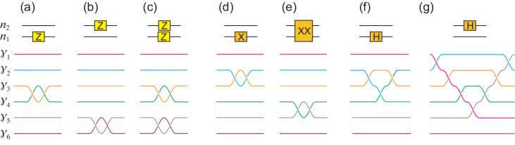
Figure S2: The braiding process for Pauli gates. (a) Pauli Z gate embedded to the first qubit, (b) Pauli Z gate embedded to the second qubit, (c) Two Pauli Z gates are embedded to the first and the second qubits, (d) Pauli X gate embedded to the first qubit, (e) Two Pauli X gates are embedded to the first and the second qubits, (f) Hadamard gate embedded to the first qubit and (g) Hadamard gate embedded to the second qubit.

S6 Pauli gates

The two-qubit Pauli gates are defined by

$$\sigma_{k_{2}}\otimes\sigma_{k_{1}},$$ (S40)

where $k_{1}$ and $k_{2}$ take $0,x,y$ and $z$. The Pauli Z gates are generated by braiding $\mathcal{B}_{2k+1}$ with odd indices,

$$I_{2}\otimes\sigma_{\text{Z}}=i\mathcal{B}_{3}^{2},\quad\sigma_{\text{Z}}\otimes I_{2}=i\mathcal{B}_{5}^{2},\quad\sigma_{\text{Z}}\otimes\sigma_{\text{Z}}=-\mathcal{B}_{5}^{2}\mathcal{B}_{3}^{2}.$$ (S41)

They are summarized as

$$\left(\sigma_{\text{Z}}\right)^{n_{2}}\otimes\left(\sigma_{\text{Z}}\right)^{n_{1}}=\left(i\mathcal{B}_{5}^{2}\right)^{n_{2}}\left(i\mathcal{B}_{3}^{2}\right)^{n_{1}},$$ (S42)

where $n_{1}$ and $n_{2}$ take $0$ or $1$.

The Pauli X gates are generated by braiding with even indices $\mathcal{B}_{2k}$,

$$I_{2}\otimes\sigma_{\text{X}}=i\mathcal{B}_{2}^{2},\quad\sigma_{\text{X}}\otimes\sigma_{\text{X}}=i\mathcal{B}_{4}^{2},\quad I_{2}\otimes\sigma_{\text{X}}=-\mathcal{B}_{4}^{2}\mathcal{B}_{2}^{2}.$$ (S43)

It should be noted that $\mathcal{B}_{4}^{2}$ does not generate $I_{2}\otimes\sigma_{\text{X}}$ but generate $\sigma_{\text{X}}\otimes\sigma_{\text{X}}$. We show the braiding for Pauli gates in Fig.S2.

Pauli Y gates are generated by sequential applications of Pauli X gates and Pauli Z gates based on the relation $U_{\text{Y}}=iU_{\text{X}}U_{\text{Z}}$. Thus, all of Pauli gates for two qubits can be generated by braiding.

S7 Hadamard gates

The Hadamard gate acting on the first qubit can be embedded as

$$I_{2}\otimes U_{\text{H}}=i\mathcal{B}_{2}\mathcal{B}_{3}\mathcal{B}_{2}.$$ (S44)

The Hadamard gate acting on the second qubit can be embedded as

$$U_{\text{H}}\otimes I_{2}=-\mathcal{B}_{1}\mathcal{B}_{2}\mathcal{B}_{3}\mathcal{B}_{4}\mathcal{B}_{3}\mathcal{B}_{2}\mathcal{B}_{1}.$$ (S45)

It requires more braiding than the previous results[6, 5], where three braiding are enough. It is due to the choice of the correspondence between the physical and logical qubits.

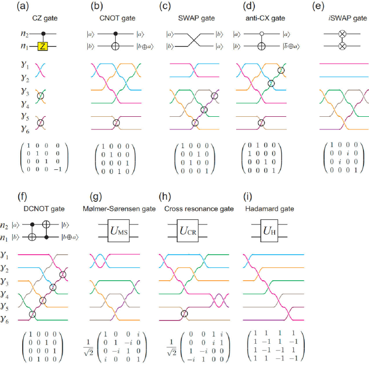
Figure S3: Braiding process for various two-qubit quantum gates. (a) CZ gate, (b) CNOT gate, (c) SWAP gate, (d) anti-CX gate, (e) $i$SWAP gate, (f) DCNOT gate, (g) Molmer-Sorensen gate, (h) cross-resonance gate (i) Hadamard gate.

S8 Quantum gates for two logical qubits

It is known that the controlled-Z (CZ) gate

$$U_{\text{CZ}}=\text{diag.}\left(1,1,1,-1\right)$$ (S46)

is generated as[6]

$$U_{\text{CZ}}=e^{-i\pi/4}\mathcal{B}_{5}^{-1}\left(\mathcal{B}_{3}\right)^{-1}\mathcal{B}_{1}.$$ (S47)

See Fig.S3(a).

It is also known that the controlled-NOT (CNOT) gate

$$U_{\text{CNOT}}=\left(\begin{array}[]{cccc}1&0&0&0\\ 0&1&0&0\\ 0&0&0&1\\ 0&0&1&0\end{array}\right)$$ (S48)

is generated by 7 braiding[4, 6, 7], wher braiding are given by

$$U_{\text{CNOT}}=-e^{-i\pi/4}\mathcal{B}_{5}^{-1}\mathcal{B}_{1}\mathcal{B}_{2}\mathcal{B}_{3}\mathcal{B}_{1}\mathcal{B}_{2}\mathcal{B}_{1}.$$ (S49)

See Fig.S3(b). On the other hand, there is a quantum circuit decomposition formula

$$U_{\text{CNOT}}=\left(I_{2}\otimes U_{\text{H}}\right)U_{\text{CZ}}\left(I_{2}\otimes U_{\text{H}}\right),$$ (S50)

which involves 9 braiding.

The SWAP gate is defined by

$$U_{\text{SWAP}}\equiv\left(\begin{array}[]{cccc}1&0&0&0\\ 0&0&1&0\\ 0&1&0&0\\ 0&0&0&1\end{array}\right),$$ (S51)

which is realized by 7 braiding as

$$U_{\text{SWAP}}=e^{i\pi/4}\left(\mathcal{B}_{3}\right)^{-1}\left(\mathcal{B}_{4}\right)^{-1}\left(\mathcal{B}_{5}\right)^{-1}\mathcal{B}_{3}\mathcal{B}_{4}\mathcal{B}_{3}\mathcal{B}_{1}.$$ (S52)

See Fig.S3(c). This is smaller than the previous result using 15 braiding[6] based on the quantum circuit decomposition

$$U_{\text{SWAP}}=\left(I_{2}\otimes U_{\text{H}}\right)U_{\text{CZ}}\left(I_{2}\otimes U_{\text{H}}\right)\left(U_{\text{H}}\otimes I_{2}\right)U_{\text{CZ}}\left(U_{\text{H}}\otimes I_{2}\right)\left(I_{2}\otimes U_{\text{H}}\right)U_{\text{CZ}}\left(I_{2}\otimes U_{\text{H}}\right).$$ (S53)

We list up various quantum gates generated by braiding.

The anti-CNOT gate is defined by[8]

$$U_{\text{\={C}X}}\equiv\left(\begin{array}[]{cccc}0&1&0&0\\ 1&0&0&0\\ 0&0&1&0\\ 0&0&0&1\end{array}\right),$$ (S54)

which is generated by 7 braiding

$$U_{\text{\={C}X}}=e^{i\pi/4}\mathcal{B}_{5}^{-1}\mathcal{B}_{1}^{-1}\mathcal{B}_{2}^{-1}\mathcal{B}_{3}\mathcal{B}_{1}\mathcal{B}_{2}\mathcal{B}_{1}.$$ (S55)

It can be decomposed into $U_{\text{\={C}X}}=\left(I_{2}\otimes U_{\text{X}}\right)U_{\text{CNOT}}$. If we use this relation, 9 braiding are necessary. See Fig.S3(d).

The $i$SWAP gate is defined by

$$U_{i\text{SWAP}}\equiv\left(\begin{array}[]{cccc}1&0&0&0\\ 0&0&i&0\\ 0&i&0&0\\ 0&0&0&1\end{array}\right),$$ (S56)

which is realized by the six braiding

$$U_{i\text{SWAP}}=-\mathcal{B}_{3}\mathcal{B}_{4}\mathcal{B}_{5}\mathcal{B}_{3}\mathcal{B}_{4}\mathcal{B}_{3}.$$ (S57)

See Fig.S3(e).

The double CNOT gate is defined by[9]

$$U_{\text{DCNOT}}\equiv\left(\begin{array}[]{cccc}1&0&0&0\\ 0&0&1&0\\ 0&0&0&1\\ 0&1&0&0\end{array}\right),$$ (S58)

which is realized by

$$U_{\text{DCNOT}}=\mathcal{B}_{2}^{-1}\mathcal{B}_{3}^{-1}\mathcal{B}_{4}^{-1}\mathcal{B}_{5}^{-1}\mathcal{B}_{1}\mathcal{B}_{2}\mathcal{B}_{3}\mathcal{B}_{4}.$$ (S59)

See Fig.S3(f).

The Mølmer-Sørensen gate is defined by[10]

$$U_{\text{MS}}\equiv\frac{1}{\sqrt{2}}\left(\begin{array}[]{cccc}1&0&0&i\\ 0&1&-i&0\\ 0&-i&1&0\\ i&0&0&1\end{array}\right),$$ (S60)

which is realized by

$$U_{\text{MS}}=-i\mathcal{B}_{3}\mathcal{B}_{4}\mathcal{B}_{5}\mathcal{B}_{4}\mathcal{B}_{3}\mathcal{B}_{1}\mathcal{B}_{1}.$$ (S61)

See Fig.S3(g).

The cross-resonance gate is defined by[11]

$$U_{\text{CR}}\equiv\frac{1}{\sqrt{2}}\left(\begin{array}[]{cccc}0&0&1&i\\ 0&0&i&1\\ 1&-i&0&0\\ -i&1&0&0\end{array}\right),$$ (S62)

which is realized by

$$U_{\text{CR}}=-\mathcal{B}_{4}\mathcal{B}_{4}\mathcal{B}_{1}\mathcal{B}_{2}\mathcal{B}_{3}\mathcal{B}_{2}\mathcal{B}_{1}.$$ (S63)

See Fig.S3(h).

We define the entangled Hadamard gate by

$$U_{\text{H}}^{\left(2\right)}=\left(\begin{array}[]{cccc}1&1&1&1\\ 1&-1&1&-1\\ 1&-1&-1&1\\ 1&1&-1&-1\end{array}\right),$$ (S64)

which is realized by

$$U_{\text{H}}^{\left(2\right)}=-e^{-i\pi/4}\mathcal{B}_{5}\mathcal{B}_{4}\mathcal{B}_{3}\mathcal{B}_{2}\mathcal{B}_{1}.$$ (S65)

See Fig.S3(i). It is different from the cross product of the Hadamard gates

$$U_{\text{H}}^{\left(2\right)}\neq U_{\text{H}}\otimes U_{\text{H}}.$$ (S66)

We note that it is obtained by a permutation of the third and fourth columns of the cross product of the Hadamard gates given by

$$U_{\text{H}}\otimes U_{\text{H}}=\left(\begin{array}[]{cccc}1&1&1&1\\ 1&-1&1&-1\\ 1&1&-1&-1\\ 1&-1&-1&1\end{array}\right),$$ (S67)

which leads to a relation

$$U_{\text{H}}\otimes U_{\text{H}}=U_{\text{CNOT}}U_{\text{H}}^{\left(2\right)}.$$ (S68)

Hence, it is realized by

$$U_{\text{H}}\otimes U_{\text{H}}=-\mathcal{B}_{5}^{-1}\mathcal{B}_{1}\mathcal{B}_{2}\mathcal{B}_{3}\mathcal{B}_{1}\mathcal{B}_{2}\mathcal{B}_{1}\mathcal{B}_{5}\mathcal{B}_{4}\mathcal{B}_{3}\mathcal{B}_{2}\mathcal{B}_{1}.$$ (S69)

Both $U_{\text{H}}^{\left(2\right)}$ and $U_{\text{H}}\otimes U_{\text{H}}$ are the Hadamard gates and they are useful for various quantum algorithms.

S9 Equal-coefficient states

The equal-coefficient state is constructed as

$$i\mathcal{B}_{1}\mathcal{B}_{2}\mathcal{B}_{3}\mathcal{B}_{4}\mathcal{B}_{5}\left|0,0\right\rangle_{\text{logical}} =\frac{1}{2}\left(\left|0,0\right\rangle_{\text{logical}}+\left|0,1\right\rangle_{\text{logical}}+\left|1,0\right\rangle_{\text{logical}}+\left|1,1\right\rangle_{\text{logical}}\right)$$

$$\equiv\frac{1}{2}\left(\left|0\right\rangle_{\text{logical}}^{\text{decimal}}+\left|1\right\rangle_{\text{logical}}^{\text{decimal}}+\left|2\right\rangle_{\text{logical}}^{\text{decimal}}+\left|3\right\rangle_{\text{logical}}^{\text{decimal}}\right),$$ (S70)

where $\left|j\right\rangle_{\text{logical}}^{\text{decimal}}$ is a decimal representation of qubits. It is a fundamental entangled state for two qubits.

S10 Three logical qubits

We use eight Majorana fermions in order to construct three logical qubits,

$$c_{1}=\frac{1}{2}\left(\gamma_{1}+i\gamma_{2}\right),\quad c_{2}=\frac{1}{2}\left(\gamma_{3}+i\gamma_{4}\right),\quad c_{3}=\frac{1}{2}\left(\gamma_{5}+i\gamma_{6}\right).\quad c_{4}=\frac{1}{2}\left(\gamma_{7}+i\gamma_{8}\right).$$ (S71)

The explicit braid actions on the physical qubits are

$$\mathcal{B}_{1} =I_{2}\otimes I_{2}\otimes I_{2}\otimes U_{\text{S}},$$

$$\mathcal{B}_{2} =I_{2}\otimes I_{2}\otimes U_{xx},$$

$$\mathcal{B}_{3} =I_{2}\otimes I_{2}\otimes U_{\text{S}}\otimes I_{2},$$

$$\mathcal{B}_{4} =I_{2}\otimes U_{xx}\otimes I_{2},$$

$$\mathcal{B}_{5} =I_{2}\otimes U_{\text{S}}\otimes I_{2}\otimes I_{2},$$

$$\mathcal{B}_{6} =U_{xx}\otimes I_{2}\otimes I_{2},$$

$$\mathcal{B}_{7} =U_{\text{S}}\otimes I_{2}\otimes I_{2}\otimes I_{2}.$$ (S72)

Three logical qubits are constructed from four physical qubits as

$$\left(\begin{array}[]{c}\left|0,0,0\right\rangle\\ \left|0,0,1\right\rangle\\ \left|0,1,0\right\rangle\\ \left|0,1,1\right\rangle\\ \left|1,0,0\right\rangle\\ \left|1,0,1\right\rangle\\ \left|1,1,0\right\rangle\\ \left|1,1,1\right\rangle\end{array}\right)_{\text{logical}}=\left(\begin{array}[]{c}\left|0,0,0,0\right\rangle\\ \left|0,0,1,1\right\rangle\\ \left|0,1,0,1\right\rangle\\ \left|0,1,1,0\right\rangle\\ \left|1,0,0,1\right\rangle\\ \left|1,0,1,0\right\rangle\\ \left|1,1,0,0\right\rangle\\ \left|1,1,1,1\right\rangle\end{array}\right)_{\text{physical}}.$$ (S73)

Explicit matrix representations for the braiding operator are

$$\mathcal{B}_{1} =e^{-i\pi/4}\text{diag.}\left(1,i,i,1,i,1,1,i\right)=\exp\left[-\frac{i\pi}{4}\sigma_{z}\otimes\sigma_{z}\otimes\sigma_{z}\right],$$

$$\mathcal{B}_{2} =I_{4}\otimes R_{x},$$

$$\mathcal{B}_{3} =e^{-i\pi/4}\text{diag.}\left(1,i,1,i,1,i,1,i\right)=e^{-i\pi/4}I_{4}\otimes U_{\text{S}},$$

$$\mathcal{B}_{4} =I_{2}\otimes U_{xx},$$

$$\mathcal{B}_{5} =e^{-i\pi/4}\text{diag.}\left(1,1,i,i,1,1,i,i\right)=e^{-i\pi/4}I_{2}\otimes U_{\text{S}}\otimes I_{2},$$

$$\mathcal{B}_{6} =U_{xx}\otimes I_{2},$$

$$\mathcal{B}_{7} =e^{-i\pi/4}\text{diag.}\left(1,1,1,1,i,i,i,i\right)=e^{-i\pi/4}U_{\text{S}}\otimes I_{4}.$$ (S74)

S11 Pauli gates

The three-qubit Pauli gates are defined by

$$\sigma_{k_{3}}\otimes\sigma_{k_{2}}\otimes\sigma_{k_{1}},$$ (S75)

where $k_{1}$, $k_{2}$ and $k_{3}$ take $0,x,y$ and $z$. The Pauli Z gates are generated by braiding operators $\mathcal{B}_{2k+1}$ with odd indices

$$I_{2}\otimes I_{2}\otimes\sigma_{\text{Z}}=i\mathcal{B}_{3}^{2},\quad I_{2}\otimes\sigma_{\text{Z}}\otimes I_{2}=i\mathcal{B}_{5}^{2},\quad\sigma_{\text{Z}}\otimes I_{2}\otimes I_{2}=i\mathcal{B}_{7}^{2},$$ (S76)

They are summarized as

$$\left(\sigma_{\text{Z}}\right)^{n_{3}}\otimes\left(\sigma_{\text{Z}}\right)^{n_{2}}\otimes\left(\sigma_{\text{Z}}\right)^{n_{1}}=\left(i\mathcal{B}_{7}^{2}\right)^{n_{3}}\left(i\mathcal{B}_{5}^{2}\right)^{n_{2}}\left(i\mathcal{B}_{3}^{2}\right)^{n_{1}},$$ (S77)

where $n_{1}$ $n_{2}$ and $n_{3}$ take $0$ or $1$.

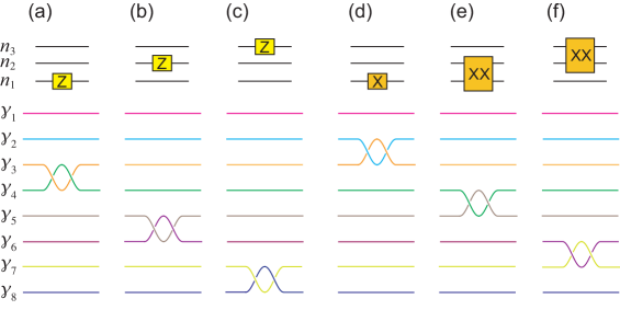
Figure S4: Pauli gates embedded in three qubits. (a) Pauli Z gate embedded to the first qubit, (b) Pauli Z gate embedded to the second qubit, (c) Pauli Z gate embedded to the third qubit, (d) Pauli X gate embedded to the first qubit, (e) Two Pauli X gates are embedded to the first and second qubits and (f) Two Pauli X gates are embedded to the second third qubits.

The Pauli X gates are generated by braiding operators with even numbers,

$$I_{2}\otimes I_{2}\otimes\sigma_{\text{X}}=i\mathcal{B}_{2}^{2},\quad I_{2}\otimes\sigma_{\text{X}}\otimes\sigma_{\text{X}}=i\mathcal{B}_{4}^{2},\quad\sigma_{\text{X}}\otimes\sigma_{\text{X}}\otimes I_{2}=i\mathcal{B}_{6}^{2}.$$ (S78)

We show the corresponding braiding in Fig.S4. It is impossible to construct logical gates corresponding to

$$I_{2}\otimes\sigma_{\text{X}}\otimes I_{2}\text{ and }\sigma_{\text{X}}\otimes I_{2}\otimes I_{2}$$ (S79)

solely by braiding. This problem is solved by introducing many-body interactions of Majorana fermions as in Eq.(S142).

The other Pauli gates can be generated by sequential applications of the above Pauli gates.

S12 Diagonal braiding

We first search braiding operators for the quantum gates generated by odd double braiding,

$$U_{\text{diag}}=\left(\mathcal{B}_{7}^{2}\right)^{n_{3}}\left(\mathcal{B}_{5}^{2}\right)^{n_{2}}\left(\mathcal{B}_{3}^{2}\right)^{n_{1}}.$$ (S80)

There are eight patterns represented by the Pauli Z gates

$$\text{diag.}\left(1,1,1,1,1,1,1,1\right) =I_{2}\otimes I_{2}\otimes I_{2},$$

$$\text{diag.}\left(1,-1,1,-1,1,-1,1,-1\right) =I_{2}\otimes I_{2}\otimes\sigma_{\text{Z}}=i\mathcal{B}_{3}^{2},$$

$$\text{diag.}\left(1,1,-1,-1,1,1,-1,-1\right) =I_{2}\otimes\sigma_{\text{Z}}\otimes I_{2}=i\mathcal{B}_{5}^{2},$$

$$\text{diag.}\left(1,1,1,1,-1,-1,-1,-1\right) =\sigma_{\text{Z}}\otimes I_{2}\otimes I_{2}=i\mathcal{B}_{7}^{2},$$

$$\text{diag.}\left(1,-1,-1,1,1,-1,-1,1\right) =I_{2}\otimes\sigma_{\text{Z}}\otimes\sigma_{\text{Z}}=-\mathcal{B}_{5}^{2}\mathcal{B}_{3}^{2},$$

$$\text{diag.}\left(1,1,-1,-1,-1,-1,1,1\right) =\sigma_{\text{Z}}\otimes\sigma_{\text{Z}}\otimes I_{2}=-\mathcal{B}_{7}^{2}\mathcal{B}_{5}^{2},$$

$$\text{diag.}\left(1,-1,1,-1,-1,1,-1,1\right) =\sigma_{\text{Z}}\otimes I_{2}\otimes\sigma_{\text{Z}}=-\mathcal{B}_{7}^{2}\mathcal{B}_{3}^{2},$$

$$\text{diag.}\left(1,-1,-1,1,-1,1,1,-1\right) =\sigma_{\text{Z}}\otimes\sigma_{\text{Z}}\otimes\sigma_{\text{Z}}=-i\mathcal{B}_{7}^{2}\mathcal{B}_{5}^{2}\mathcal{B}_{3}^{2}.$$ (S81)

Next, we search real and diagonal gates obtained by the following odd braiding

$$\left(\mathcal{B}_{7}\right)^{n_{3}}\left(\mathcal{B}_{5}\right)^{n_{2}}\left(\mathcal{B}_{3}\right)^{n_{1}}.$$ (S82)

We search states whose components are $\pm 1$. There are four additional quantum gates, whose traces are zero Tr$U_{\text{diag}}=0$,

$$\text{diag.}\left(1,-1,-1,-1,1,1,1,-1\right)=i\mathcal{B}_{4}^{-1}\mathcal{B}_{3}\mathcal{B}_{2}\mathcal{B}_{1},$$

$$\text{diag.}\left(1,-1,1,1,-1,-1,1,-1\right)=i\mathcal{B}_{3}^{-1}\mathcal{B}_{4}\mathcal{B}_{2}\mathcal{B}_{1},$$

$$\text{diag.}\left(1,1,-1,1,-1,1,-1,-1\right)=i\mathcal{B}_{2}^{-1}\mathcal{B}_{3}\mathcal{B}_{4}\mathcal{B}_{1},$$

$$\text{diag.}\left(1,1,1,-1,1,-1,-1,-1\right)=-i\mathcal{B}_{4}^{-1}\mathcal{B}_{3}^{-1}\mathcal{B}_{2}^{-1}\mathcal{B}_{1}.$$ (S83)

In addition, there are additional quantum gates, whose traces are nonzero Tr$U_{\text{diag}}\neq 0$,

$$\text{diag.}\left(1,-1,-1,-1,-1,-1,-1,1\right)=-\mathcal{B}_{4}\mathcal{B}_{3}\mathcal{B}_{2}\mathcal{B}_{1},$$

$$\text{diag.}\left(1,-1,1,1,1,1,-1,1\right)=\mathcal{B}_{4}^{-1}\mathcal{B}_{3}^{-1}\mathcal{B}_{2}\mathcal{B}_{1},$$

$$\text{diag.}\left(1,1,-1,1,1,-1,1,1\right)=\mathcal{B}_{4}^{-1}\mathcal{B}_{2}^{-1}\mathcal{B}_{3}\mathcal{B}_{1},$$

$$\text{diag.}\left(1,1,1,-1,-1,1,1,1\right)=\mathcal{B}_{3}^{-1}\mathcal{B}_{2}^{-1}\mathcal{B}_{4}\mathcal{B}_{1}.$$ (S84)

It is natural to anticipate that the CZ gate and the CCZ gate are generated by even braiding because they are diagonal gates. However, this is not the case by checking all $4^{3}$ patterns of braiding. As a result, the even braiding do not generate the CZ gates

$$I_{2}\otimes U_{\text{CZ}} =\text{diag.}\left(1,1,1,-1,1,1,1,-1\right),$$

$$U_{\text{CZ}}\otimes I_{2} =\text{diag.}\left(1,1,1,1,1,1,-1,-1\right),$$ (S85)

and the CCZ gate

$$U_{\text{CCZ}}=\text{diag.}\left(1,1,1,1,1,1,1,-1\right).$$ (S86)

This problem is solved by introducing many-body interactions of Majorana fermions as shown in the main text.

S13 Hadamard gates

The Hadamard gate can be embedded in the first qubit as

$$I_{2}\otimes I_{2}\otimes U_{\text{H}}=i\mathcal{B}_{2}\mathcal{B}_{3}\mathcal{B}_{2},$$ (S87)

as in the case of (S44). We also find that the Hadamard gate can be embedded in the third qubit as

$$U_{\text{H}}\otimes I_{2}\otimes I_{2}=-i\mathcal{B}_{1}\mathcal{B}_{2}\mathcal{B}_{3}\mathcal{B}_{4}\mathcal{B}_{5}\mathcal{B}_{6}\mathcal{B}_{5}\mathcal{B}_{4}\mathcal{B}_{3}\mathcal{B}_{2}\mathcal{B}_{1}.$$ (S88)

On the other hand, it is very hard to embed the Hadamard gate in the second qubit $I_{2}\otimes U_{\text{H}}\otimes I_{2}$. It is possible by introducing many-body interactions of Majorana fermions. The Hadamard gate for the $N$-th qubit is given by

$$U_{\text{H}}\otimes I_{2N-2}\propto\mathcal{B}_{1}\mathcal{B}_{2}\cdots\mathcal{B}_{2N-1}\mathcal{B}_{2N}\mathcal{B}_{2N-1}\cdots\mathcal{B}_{2}\mathcal{B}_{1}.$$ (S89)

S14 Two-qubit quantum gates embedded in three-qubit quantum gates

The $i$SWAP gate can be embedded to a three-qubit topological gate because it does not involve $\mathcal{B}_{1}$ and is given by

$$I_{2}\otimes U_{i\text{SWAP}}=-\mathcal{B}_{3}\mathcal{B}_{4}\mathcal{B}_{5}\mathcal{B}_{3}\mathcal{B}_{4}\mathcal{B}_{3}.$$ (S90)

See Fig.S5(a). We also find the $i$SWAP gate can be embedded as

$$U_{i\text{SWAP}}\otimes I_{2}=-\mathcal{B}_{5}\mathcal{B}_{6}\mathcal{B}_{7}\mathcal{B}_{5}\mathcal{B}_{6}\mathcal{B}_{5}.$$ (S91)

See Fig.S5(b).

S15 Three-qubit quantum gates

We find that the three-qubit Hadamard transformation is generated as

$$U_{\text{H}}^{\left(3\right)}=-\mathcal{B}_{7}\mathcal{B}_{6}\mathcal{B}_{5}\mathcal{B}_{4}\mathcal{B}_{3}\mathcal{B}_{2}\mathcal{B}_{1}=\left(\begin{array}[]{cccccccc}1&1&1&1&1&1&1&1\\ 1&-1&1&-1&1&-1&1&-1\\ 1&-1&-1&1&1&-1&-1&1\\ 1&1&-1&-1&1&1&-1&-1\\ 1&-1&-1&1&-1&1&1&-1\\ 1&1&-1&-1&-1&-1&1&1\\ 1&1&1&1&-1&-1&-1&-1\\ 1&-1&1&-1&-1&1&-1&1\end{array}\right).$$ (S92)

See Fig.S5(b). It is different from the cross-product of the Hadamard gate

$$U_{\text{H}}\otimes U_{\text{H}}\otimes U_{\text{H}}=\left(\begin{array}[]{cccccccc}1&1&1&1&1&1&1&1\\ 1&-1&1&-1&1&-1&1&-1\\ 1&1&-1&-1&1&1&-1&-1\\ 1&-1&-1&1&1&-1&-1&1\\ 1&1&1&1&-1&-1&-1&-1\\ 1&-1&1&-1&-1&1&-1&1\\ 1&1&-1&-1&-1&-1&1&1\\ 1&-1&-1&1&-1&1&1&-1\end{array}\right).$$ (S93)

There is a relation

$$U_{\text{H}}\otimes U_{\text{H}}\otimes U_{\text{H}}=-U_{3\text{P}}U_{\text{H}}^{\left(3\right)},$$ (S94)

where $U_{3\text{P}}$ is defined by

$$U\equiv\left(\begin{array}[]{cccccccc}1&0&0&0&0&0&0&0\\ 0&1&0&0&0&0&0&0\\ 0&0&0&1&0&0&0&0\\ 0&0&1&0&0&0&0&0\\ 0&0&0&0&0&0&1&0\\ 0&0&0&0&0&0&0&1\\ 0&0&0&0&0&1&0&0\\ 0&0&0&0&1&0&0&0\end{array}\right).$$ (S95)

It is impossible to generate the W state by braiding

$$\left|\text{W}\right\rangle_{\text{logical}}=\frac{1}{\sqrt{3}}\left(\left|000\right\rangle_{\text{logical}}+\left|010\right\rangle_{\text{logical}}+\left|100\right\rangle_{\text{logical}}\right),$$ (S96)

because the number of the nonzero terms of the W state is 3, which contradicts the fact that the number of the nonzero terms must be $1$, $2$, $4$ and $8$ for three qubit states generated by braiding.

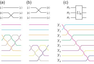
Figure S5: (a) and (b) $i$SWAP gate embedded to three qubit systems. (c) Three-qubit Hadamard transformation.

S16 $N$ logical qubits

The braid representation of $2N+2$ Majorana fermions is equivalent to the $\pi/2$ rotation in SO$\left(2N+2\right)$, suggested by the fact that braid operators are represented by the Gamma matrices[12, 13]. The number of the braid group is given by[14]

$$\left|\text{Image}\left(\mathcal{B}_{2n}\right)\right|=\left\{\begin{array}[]{ccc}2^{2n-1}\left(2n\right)!&\text{for}&n\text{=even}\\ 2^{2n}\left(2n\right)!&\text{for}&n\text{=odd}\end{array}\right..$$ (S97)

The $i$SWAP gate is embedded as

$$I_{2}^{k-2}\otimes U_{i\text{SWAP}}\otimes I_{2}^{N-k}\propto\mathcal{B}_{2k+1}\mathcal{B}_{2k+2}\mathcal{B}_{2k+3}\mathcal{B}_{2k+1}\mathcal{B}_{2k+2}\mathcal{B}_{2k+1}.$$ (S98)

S16.1 Diagonal braiding

We consider odd braiding defined by

$$\mathcal{B}_{\text{odd}}\left(n_{1},n_{2},\cdots,n_{k}\right)\equiv\mathcal{B}_{2n_{k}-1}\mathcal{B}_{2n_{k-1}-1}\cdots\mathcal{B}_{2n_{1}-1},$$ (S99)

where $n_{k}$ is an integer satisfying $1\leq n_{k}\leq N+1$. They are Abelian braiding because there are no adjacent braiding. Then, there are only $4^{k}$ patterns. Especially, we consider odd double braiding defined by

$$\left(\mathcal{B}_{\text{odd}}\right)^{2}\equiv\left(i\mathcal{B}_{2n_{k}-1}^{2}\right)\left(i\mathcal{B}_{2n_{k-1}-1}^{2}\right)\cdots\left(i\mathcal{B}_{2n_{1}-1}^{2}\right)$$ (S100)

are interesting because they are identical to

$$\left(\mathcal{B}_{\text{odd}}\right)^{2}=\left(\sigma_{\text{Z}}\right)^{m_{k}}\left(\sigma_{\text{Z}}\right)^{m_{2}}\cdots\left(\sigma_{\text{Z}}\right)^{m_{1}},$$ (S101)

where $m_{k}=0,1$. Namely, every Pauli gates constructing from the Pauli Z gate can be generated.

Next, we consider even braiding defined by

$$\mathcal{B}_{\text{even}}\left(n_{1},n_{2},\cdots,n_{k}\right)\equiv\mathcal{B}_{2n_{k}}\mathcal{B}_{2n_{k-1}}\cdots\mathcal{B}_{2n_{1}}.$$ (S102)

They are also the Abelian braiding, where each braiding commutes each other. We also consider even double braiding defined by

$$\left(\mathcal{B}_{\text{even}}\right)^{2}\equiv\left(i\mathcal{B}_{2n_{k}}^{2}\right)\left(i\mathcal{B}_{2n_{k-1}}^{2}\right)\cdots\left(i\mathcal{B}_{2n_{1}}^{2}\right).$$ (S103)

On the other hand, it is impossible to construct the Pauli X gate except for the first qubit. See Eq.(24) in the main text.

S16.2 Hadamard transformation

The Hadamard transformation is used for the initial process of various quantum algorithm such as the Kitaev phase estimation algorithm, the Deutsch algorithm, the Deutsch-Jozsa algorithm, the Simon algorithm, the Bernstein-Vazirani algorithm, the Grover algorithm and the Shor algorithm. It is generated by the braiding

$$U_{\text{H}}^{\left(N\right)}\propto\mathcal{B}_{2N+1}\mathcal{B}_{2N}\cdots\mathcal{B}_{2}\mathcal{B}_{1}.$$ (S104)

The equal-coefficient state is generated as

$$U_{\text{H}}^{\left(N\right)}\left|0,0\right\rangle_{\text{logical}}\propto\sum_{j=1}^{2^{N}}\left|j\right\rangle_{\text{logical}},$$ (S105)

where $\left|j\right\rangle_{\text{logical}}$ is the decimal representation of the qubit.

II $2N$-body unitary evolution

S1 Quantum gates for one logical qubit

The $2$-body Majorana operator $\mathcal{B}_{1}\left(\theta\right)$ is written in terms of fermion operators,

$$\mathcal{B}_{1}\left(\theta\right)=\cos\theta+\gamma_{2}\gamma_{1}\sin\theta=\left(\cos\theta+\left(ic_{1}^{\dagger}c_{1}-ic_{1}c_{1}^{\dagger}\right)\sin\theta\right),$$ (S106)

which operates on two physical qubits (S10) as

$$\mathcal{B}_{1}\left(\theta\right)\Psi_{\text{physical}}=\left(\begin{array}[]{cccc}e^{-i\theta}&0&0&0\\ 0&e^{i\theta}&0&0\\ 0&0&e^{-i\theta}&0\\ 0&0&0&e^{i\theta}\end{array}\right)\left(\begin{array}[]{c}\left|0,0\right\rangle\\ \left|0,1\right\rangle\\ \left|1,0\right\rangle\\ \left|1,1\right\rangle\end{array}\right)_{\text{physical}}.$$ (S107)

Taking the even parity basis, the action is

$$\mathcal{B}_{1}\left(\theta\right)\Psi_{\text{logical}}=e^{-i\theta}\left(\begin{array}[]{cc}1&0\\ 0&e^{2i\theta}\end{array}\right)\left(\begin{array}[]{c}\left|0\right\rangle\\ \left|1\right\rangle\end{array}\right)_{\text{logical}}.$$ (S108)

It is the arbitrary phase-shift gate. Especially, by setting $\theta=\pi/8$, the T gate is constructed

$$U_{\text{T}}\equiv\text{diag.}\left(1,e^{i\pi/4}\right).$$ (S109)

It is identical to the rotation along the $z$ axis

$$\mathcal{B}_{1}\left(\theta\right)=R_{z}\left(2\theta\right),$$ (S110)

with

$$R_{z}\left(\theta\right)\equiv\exp\left[-i\frac{\theta}{2}\sigma_{z}\right]=\left(\begin{array}[]{cc}e^{-i\theta/2}&0\\ 0&e^{i\theta/2}\end{array}\right).$$ (S111)

The operator $\mathcal{B}_{2}$ is written in terms of fermion operators,

$$\mathcal{B}_{2}\left(\theta\right)=\cos\theta+\gamma_{3}\gamma_{2}\sin\theta=\cos\theta+\left(ic_{2}c_{1}^{\dagger}+ic_{2}^{\dagger}c_{1}^{\dagger}-ic_{2}c_{1}-ic_{2}^{\dagger}c_{1}\right)\sin\theta,$$ (S112)

which operates on two physical qubits (S10) as[2],

$$\mathcal{B}_{2}\left(\theta\right)\Psi_{\text{physical}}=\left(\begin{array}[]{cccc}\cos\theta&0&0&-i\sin\theta\\ 0&\cos\theta&-i\sin\theta&0\\ 0&-i\sin\theta&\cos\theta&0\\ -i\sin\theta&0&0&\cos\theta\end{array}\right)\left(\begin{array}[]{c}\left|0,0\right\rangle\\ \left|0,1\right\rangle\\ \left|1,0\right\rangle\\ \left|1,1\right\rangle\end{array}\right)_{\text{physical}}.$$ (S113)

In the even parity basis, the action is

$$\mathcal{B}_{2}\left(\theta\right)=\left(\begin{array}[]{cc}\cos\theta&-i\sin\theta\\ -i\sin\theta&\cos\theta\end{array}\right)\equiv R_{x}\left(2\theta\right),$$ (S114)

which is identical to the rotation along the $x$ axis

$$\mathcal{B}_{2}\left(\theta\right)=R_{x}\left(2\theta\right),$$ (S115)

with

$$R_{x}\left(\theta\right)\equiv\exp\left[-i\frac{\theta}{2}\sigma_{x}\right]=\left(\begin{array}[]{cc}\cos\frac{\theta}{2}&-i\sin\frac{\theta}{2}\\ -i\sin\frac{\theta}{2}&\cos\frac{\theta}{2}\end{array}\right).$$ (S116)

The operator $\mathcal{B}_{3}\left(\theta\right)$ is written in terms of fermion operators

$$\mathcal{B}_{3}\left(\theta\right)=\cos\theta+\gamma_{4}\gamma_{3}\sin\theta=\cos\theta+\left(ic_{2}^{\dagger}c_{2}-ic_{2}c_{2}^{\dagger}\right)\sin\theta,$$ (S117)

which operates on two physical qubits (S10) as[2]

$$\mathcal{B}_{3}\left(\theta\right)\Psi_{\text{physical}}=\left(\begin{array}[]{cccc}e^{-i\theta}&0&0&0\\ 0&e^{-i\theta}&0&0\\ 0&0&e^{i\theta}&0\\ 0&0&0&e^{i\theta}\end{array}\right)\left(\begin{array}[]{c}\left|0,0\right\rangle\\ \left|0,1\right\rangle\\ \left|1,0\right\rangle\\ \left|1,1\right\rangle\end{array}\right)_{\text{physical}}.$$ (S118)

In the even parity basis, the action is the same as (S108),

$$\mathcal{B}_{3}\left(\theta\right)=e^{-i\theta}\left(\begin{array}[]{cc}1&0\\ 0&e^{2i\theta}\end{array}\right)\left(\begin{array}[]{c}\left|0\right\rangle\\ \left|1\right\rangle\end{array}\right)_{\text{logical}}.$$ (S119)

The rotation along the $y$ axis defined by

$$R_{y}\left(\theta\right)\equiv\exp\left[-i\frac{\theta}{2}\sigma_{y}\right]$$ (S120)

is realized by the sequential operations

$$R_{y}\left(\theta\right)=R_{z}\left(\frac{\pi}{2}\right)R_{x}\left(\theta\right)R_{z}\left(-\frac{\pi}{2}\right).$$ (S121)

S2 Three physical qubits

Next, we study the six Majorana fermion system. The explicit actions on the physical qubits are

$$\mathcal{B}_{1}\left(\theta\right) =I_{2}\otimes I_{2}\otimes R_{z}\left(2\theta\right),$$

$$\mathcal{B}_{2}\left(\theta\right) =I_{2}\otimes U_{xx}\left(\theta\right),$$

$$\mathcal{B}_{3}\left(\theta\right) =I_{2}\otimes R_{z}\left(2\theta\right)\otimes I_{2},$$

$$\mathcal{B}_{4}\left(\theta\right) =U_{xx}\otimes I_{2},$$

$$\mathcal{B}_{5}\left(\theta\right) =R_{z}\left(2\theta\right)\otimes I_{2}\otimes I_{2}.$$ (S122)

S3 Two logical qubits

Two logical qubits are constructed from three physical qubits by taking the even parity basis. The action of $\mathcal{B}_{1}\left(\theta\right)$ to the logical qubit is

$$\mathcal{B}_{1}\left(\theta\right)=\text{diag.}\left(e^{-i\theta},e^{i\theta},e^{i\theta},e^{-i\theta}\right),$$ (S123)

which is identical to the ZZ interaction

$$\mathcal{B}_{1}\left(\theta\right)=U_{zz}\left(2\theta\right),$$ (S124)

with

$$U_{zz}\left(\theta\right)\equiv\exp\left[-i\frac{\theta}{2}\sigma_{z}\otimes\sigma_{z}\right].$$ (S125)

The action of $\mathcal{B}_{4}\left(\theta\right)$ to the logical qubit is

$$\mathcal{B}_{4}\left(\theta\right)=\left(\begin{array}[]{cccc}\cos\theta&0&0&-i\sin\theta\\ 0&\cos\theta&-i\sin\theta&0\\ 0&-i\sin\theta&\cos\theta&0\\ -i\sin\theta&0&0&\cos\theta\end{array}\right),$$ (S126)

which is identical to the xx interaction

$$\mathcal{B}_{4}\left(\theta\right)=U_{xx}\left(2\theta\right),$$ (S127)

with

$$U_{xx}\left(\theta\right)\equiv\exp\left[-i\frac{\theta}{2}\sigma_{x}\otimes\sigma_{x}\right].$$ (S128)

The action of $\mathcal{B}_{3}\left(\theta\right)$ and $\mathcal{B}_{5}\left(\theta\right)$ to the logical qubit is

$$\mathcal{B}_{3}\left(\theta\right) = \text{diag.}\left(e^{-i\theta},e^{i\theta},e^{-i\theta},e^{i\theta}\right)=I_{2}\otimes U_{z}\left(\theta\right),$$

$$\mathcal{B}_{5}\left(\theta\right) = \text{diag.}\left(e^{-i\theta},e^{-i\theta},e^{i\theta},e^{i\theta}\right)=U_{z}\left(\theta\right)\otimes I_{2}.$$ (S129)

The action of $\mathcal{B}_{2}\left(\theta\right)$ to the logical qubit is

$$\mathcal{B}_{2}\left(\theta\right)=\left(\begin{array}[]{cccc}\cos\theta&-i\sin\theta&0&0\\ -i\sin\theta&\cos\theta&0&0\\ 0&0&\cos\theta&-i\sin\theta\\ 0&0&-i\sin\theta&\cos\theta\end{array}\right),$$ (S130)

which is rewritten in the form of

$$\mathcal{B}_{2}\left(\theta\right) = I_{2}\otimes R_{x}\left(2\theta\right),$$

$$\mathcal{B}_{2345}\left(\theta\right) = R_{x}\left(2\theta\right)\otimes I_{2}.$$ (S131)

S4 Controlled phase-shift gate

We find

$$\mathcal{B}_{6}\left(\theta_{3}\right)\mathcal{B}_{3}\left(\theta_{2}\right)\mathcal{B}_{1}\left(\theta_{1}\right)=\text{diag.}\left(e^{-i\left(\theta_{1}+\theta_{2}+\theta_{3}\right)},e^{i\left(\theta_{1}+\theta_{2}-\theta_{3}\right)},e^{i\left(\theta_{1}-\theta_{2}+\theta_{3}\right)},e^{i\left(-\theta_{1}+\theta_{2}+\theta_{3}\right)}\right).$$ (S132)

The controlled phase-shift gate with arbitrary phase is constructed by setting $\theta_{1}=-\theta_{2}=-\theta_{3}=-\theta$,

$$\mathcal{B}_{5}\left(-\theta\right)\mathcal{B}_{3}\left(\theta\right)\mathcal{B}_{1}\left(\theta\right)=\text{diag.}\left(e^{-i\theta},e^{-i\theta},e^{-i\theta},e^{3i\theta}\right)=e^{-i\theta}\text{diag.}\left(1,1,1,e^{4i\theta}\right).$$ (S133)

Especially, the CZ gate is constructed by setting $\theta=\pi/4.$

S5 Controlled-unitary gate

It is known that the controlled unitary gate is constructed as[22]

$$U_{\text{C-}U}=\left(I_{2}\otimes U_{A}\right)U_{\text{CNOT}}\left(I_{2}\otimes U_{B}\right)U_{\text{CNOT}}\left(I_{2}\otimes U_{C}\right)$$ (S134)

with

$$U_{A}\equiv R_{z}\left(\beta\right)R_{y}\left(\frac{\gamma}{2}\right),\qquad U_{B}\equiv R_{y}\left(-\frac{\gamma}{2}\right)R_{z}\left(-\frac{\beta+\delta}{2}\right),\qquad U_{C}\equiv R_{z}\left(\frac{\delta-\beta}{2}\right),$$ (S135)

because

$$U_{A}U_{B}U_{C}=I_{4}$$ (S136)

and

$$U_{A}XU_{B}XU_{C}=R_{z}\left(\beta\right)R_{y}\left(\gamma\right)R_{z}\left(\delta\right)=U_{\text{1bit}}.$$ (S137)

In the Majorana system, the basic rotations are not along the $y$ axis but the $x$ axis. The similar decomposition is possible only by using the rotations along the $z$ and $x$ axes as

$$U_{A}=R_{z}\left(\beta+\frac{\pi}{2}\right)R_{x}\left(\frac{\gamma}{2}\right),\qquad U_{B}=R_{x}\left(-\frac{\gamma}{2}\right)R_{z}\left(-\frac{\beta+\delta}{2}\right),\qquad U_{C}=R_{z}\left(\frac{\delta-\beta-\pi}{2}\right).$$ (S138)

The proof is similar. First, we have

$$U_{A}U_{B}U_{C}=1,$$

where we have used the relation

$$R_{j}\left(\theta_{1}\right)R_{j}\left(\theta_{2}\right)=R_{j}\left(\theta_{1}+\theta_{2}\right)$$ (S139)

for $j=x,y$ and $z$. Next, we have

$$U_{A}XU_{B}XU_{C}=U_{\text{1bit}},$$

where we have used the relation

$$R\left(\theta\right)X=XR\left(-\theta\right).$$ (S140)

Hence, the controlled unitary gate is implemented by $2$-body Majorana interaction.

S6 Four physical qubits

We consider eight Majorana fermion system The explicit actions on four physical qubits are given by

$$\mathcal{B}_{1} =I_{8}\otimes R_{z}\left(2\theta\right),$$

$$\mathcal{B}_{2} =I_{4}\otimes U_{xx}\left(\theta\right),$$

$$\mathcal{B}_{3} =I_{4}\otimes R_{z}\left(2\theta\right)\otimes I_{2},$$

$$\mathcal{B}_{4} =I_{2}\otimes U_{xx}\left(\theta\right)\otimes I_{2},$$

$$\mathcal{B}_{5} =I_{2}\otimes R_{z}\left(2\theta\right)\otimes I_{4},$$

$$\mathcal{B}_{6} =U_{xx}\left(\theta\right)\otimes I_{4},$$

$$\mathcal{B}_{7} =R_{z}\left(2\theta\right)\otimes I_{8}.$$ (S141)

We summarize results on constructing full set of Pauli Z gate for three logical qubits in  the following table:

4 physical qubits 3 logical qubits

$$\quad\mathcal{B}_{12}\left(\theta\right)$$

(S142)

We have the identical logical qubits:

$$\mathcal{B}_{12}\left(\theta\right) \simeq \mathcal{B}_{345678}\left(\theta\right),\qquad\mathcal{B}_{34}\left(\theta\right)\simeq\mathcal{B}_{125678}\left(\theta\right),\qquad\mathcal{B}_{56}\left(\theta\right)\simeq\mathcal{B}_{123478}\left(\theta\right),\qquad\mathcal{B}_{78}\left(\theta\right)\simeq\mathcal{B}_{123456}\left(\theta\right),$$

$$\mathcal{B}_{1234}\left(\theta\right) \simeq \mathcal{B}_{5678}\left(\theta\right),\qquad\mathcal{B}_{1256}\left(\theta\right)\simeq\mathcal{B}_{3478}\left(\theta\right),\qquad\mathcal{B}_{1278}\left(\theta\right)\simeq\mathcal{B}_{3456}\left(\theta\right).$$ (S143)

S7 Three logical qubits

Three logical qubits are constructed from four physical qubits by taking the even parity basis.

$$\mathcal{B}_{12} = \text{diag.}\left(e^{-i\theta},e^{i\theta},e^{i\theta},e^{-i\theta},e^{i\theta},e^{-i\theta},e^{-i\theta},e^{i\theta}\right)=\exp\left[-i\theta\sigma_{z}\otimes\sigma_{z}\otimes\sigma_{z}\right],$$

$$\mathcal{B}_{23} = I_{2}\otimes I_{2}\otimes R_{x}\left(2\theta\right),$$

$$\mathcal{B}_{34} = I_{2}\otimes I_{2}\otimes R_{z}\left(2\theta\right)=\exp\left[-i\theta I_{2}\otimes I_{2}\otimes\sigma_{z}\right],$$

$$\mathcal{B}_{45} = I_{2}\otimes U_{xx}\left(2\theta\right),$$

$$\mathcal{B}_{56} = I_{2}\otimes R_{z}\left(2\theta\right)\otimes I_{2}=\exp\left[-i\theta I_{2}\otimes\sigma_{z}\otimes I_{2}\right],$$

$$\mathcal{B}_{67} = U_{xx}\left(2\theta\right)\otimes I_{2},$$

$$\mathcal{B}_{78} = R_{z}\left(2\theta\right)\otimes I_{4}.$$ (S144)

We find that controlled-controlled phase shift gate cannot be implemented only by diagonal braiding. It is proved by counting the number of the degrees of freedom. We need to tune 7 parameters for the diagonal quantum gates. On the other hand, there are only three independent angle because the diagonal operators are $\mathcal{B}_{1}$, $\mathcal{B}_{3}$ and $\mathcal{B}_{5}$. Hence, it is impossible to construct controlled-controlled phase shift gate in general. However, this problem is solved by introducing many-body Majorana interaction,

$$U_{\text{CC}\phi}=\mathcal{B}_{12}\left(\frac{\phi}{8}\right)\mathcal{B}_{34}\left(\frac{\phi}{8}\right)\mathcal{B}_{56}\left(\frac{\phi}{8}\right)\mathcal{B}_{78}\left(\frac{\phi}{8}\right)\mathcal{B}_{1234}^{\left(4\right)}\left(-\frac{\phi}{8}\right)\mathcal{B}_{1278}^{\left(4\right)}\left(-\frac{\phi}{8}\right)\mathcal{B}_{1256}^{\left(4\right)}\left(-\frac{\phi}{8}\right).$$ (S145)

Especially, the CCZ gate is constructed as follows

$$U_{\text{CCZ}}=\mathcal{B}_{12}\left(\frac{\pi}{8}\right)\mathcal{B}_{34}\left(\frac{\pi}{8}\right)\mathcal{B}_{56}\left(\frac{\pi}{8}\right)\mathcal{B}_{78}\left(\frac{\pi}{8}\right)\mathcal{B}_{1234}^{\left(4\right)}\left(-\frac{\pi}{8}\right)\mathcal{B}_{1278}^{\left(4\right)}\left(-\frac{\pi}{8}\right)\mathcal{B}_{1256}^{\left(4\right)}\left(-\frac{\pi}{8}\right).$$ (S146)

The Toffoli gate is constructed by applying the Hadamard gate to the CCZ gate as in

$$U_{\text{Toffloi}}=\left(I_{4}\otimes U_{\text{H}}\right)U_{\text{CCZ}}\left(I_{4}\otimes U_{\text{H}}\right).$$ (S147)

See Fig.1(a).

The Fredkin gate is constructed by sequential applications of three Toffoli gates as in

$$U_{\text{Fredkin}}=U_{\text{Toffoli}}^{\left(3,2\right)\rightarrow 1}U_{\text{Toffoli}}^{\left(3,1\right)\rightarrow 2}U_{\text{Toffoli}}^{\left(3,2\right)\rightarrow 1}.$$ (S148)

See Fig.1(b).

The CZ gate in three qubits are embedded as

$$U_{\text{CZ}}^{3\rightarrow 2} = \mathcal{B}_{56}\left(\frac{\pi}{4}\right)\mathcal{B}_{78}\left(\frac{\pi}{4}\right)\mathcal{B}_{1234}^{\left(4\right)}\left(-\frac{\pi}{4}\right),$$

$$U_{\text{CZ}}^{3\rightarrow 1} = \mathcal{B}_{34}\left(\frac{\pi}{4}\right)\mathcal{B}_{78}\left(\frac{\pi}{4}\right)\mathcal{B}_{1234}^{\left(4\right)}\left(-\frac{\pi}{4}\right),$$

$$U_{\text{CZ}}^{2\rightarrow 1} = \mathcal{B}_{34}\left(\frac{\pi}{4}\right)\mathcal{B}_{56}\left(\frac{\pi}{4}\right)\mathcal{B}_{1278}^{\left(4\right)}\left(-\frac{\pi}{4}\right).$$ (S149)

S8 Logical 4 qubits

We summarize results on constructing full set of Pauli Z gate for four logical qubits in  the following table:

4 logical qubits

$$\quad\mathcal{B}_{12}\left(\theta\right)$$

(S150)

where $0$ is an abbreviation of $10$. The CCC$\phi$ gate is explicitly constructed as

$$U_{\text{C}^{3}\phi}=\mathcal{B}_{34}\left(\frac{\phi}{16}\right)\mathcal{B}_{56}\left(\frac{\phi}{16}\right)\mathcal{B}_{78}\left(\frac{\phi}{16}\right)\mathcal{B}_{90}\left(\frac{\phi}{16}\right)\mathcal{B}_{1234}^{\left(4\right)}\left(\frac{\phi}{16}\right)\mathcal{B}_{1256}^{\left(4\right)}\left(\frac{\phi}{16}\right)\mathcal{B}_{1278}^{\left(4\right)}\left(\frac{\phi}{16}\right)\mathcal{B}_{1290}^{\left(4\right)}\left(\frac{\phi}{16}\right)$$

$$\mathcal{B}_{3456}^{\left(4\right)}\left(-\frac{\phi}{16}\right)\mathcal{B}_{3478}^{\left(4\right)}\left(-\frac{\phi}{16}\right)\mathcal{B}_{3490}^{\left(4\right)}\left(-\frac{\phi}{16}\right)\mathcal{B}_{5678}^{\left(4\right)}\left(\frac{\phi}{16}\right)\mathcal{B}_{5690}^{\left(4\right)}\left(-\frac{\phi}{16}\right)\mathcal{B}_{7890}^{\left(4\right)}\left(-\frac{\phi}{16}\right)\mathcal{B}_{12}^{\left(4\right)}\left(-\frac{\phi}{16}\right).$$ (S151)

S9 Generalized braid group relation

We consider the case $\theta=\pi/4$. The Artin braid group relation reads[1],

$$\mathcal{B}_{\alpha}\mathcal{B}_{\beta}=\mathcal{B}_{\beta}\mathcal{B}_{\alpha}\qquad\text{for\quad}\left|\alpha-\beta\right|\geq 2,\qquad\mathcal{B}_{\alpha}\mathcal{B}_{\alpha+1}\mathcal{B}_{\alpha}=\mathcal{B}_{\alpha+1}\mathcal{B}_{\alpha}\mathcal{B}_{\alpha+1}.$$ (S152)

It is identical to the extraspecial 2 group[23]

$$M_{\alpha}^{2} = -1,\qquad M_{\alpha}M_{\alpha+1}=-M_{\alpha+1}M_{\alpha},$$

$$M_{a}M_{\beta} = M_{\beta}M_{\alpha},\qquad\text{for\quad}\left|\alpha-\beta\right|\geq 2,$$ (S153)

by setting

$$\mathcal{B}_{\alpha}^{\left(4\right)}=\frac{1}{\sqrt{2}}\left(1+M_{\alpha}\right).$$ (S154)

It is straightforward to show that

$$\left(M_{\alpha}^{\left(4\right)}\right)^{2} = -1,$$

$$M_{\alpha}^{\left(4\right)}M_{\alpha+1}^{\left(4\right)} = -M_{\alpha+1}^{\left(4\right)}M_{\alpha}^{\left(4\right)},$$

$$M_{\alpha}^{\left(4\right)}M_{\alpha+2}^{\left(4\right)} = M_{\alpha+2}^{\left(4\right)}M_{\alpha}^{\left(4\right)},$$

$$M_{\alpha}^{\left(4\right)}M_{\alpha+3}^{\left(4\right)} = -M_{\alpha+3}^{\left(4\right)}M_{\alpha}^{\left(4\right)},$$

$$M_{a}^{\left(4\right)}M_{\beta}^{\left(4\right)} = M_{\beta}^{\left(4\right)}M_{\alpha}^{\left(4\right)}\quad\text{for}\quad\left|\alpha-\beta\right|\geq 4,$$ (S155)

when we set

$$M_{\alpha}^{\left(4\right)}\equiv i\gamma_{4}\gamma_{3}\gamma_{2}\gamma_{1}.$$ (S156)

It is a generalization of the extraspecial 2 group. Correspondingly, we obtain a generalized braiding group relation

$$\mathcal{B}_{\alpha}^{\left(4\right)}\mathcal{B}_{\alpha+1}^{\left(4\right)}\mathcal{B}_{\alpha}^{\left(4\right)}=\mathcal{B}_{\alpha+1}^{\left(4\right)}\mathcal{B}_{\alpha}^{\left(4\right)}\mathcal{B}_{\alpha+1}^{\left(4\right)},\qquad\mathcal{B}_{\alpha}^{\left(4\right)}\mathcal{B}_{\alpha+3}^{\left(4\right)}\mathcal{B}_{\alpha}^{\left(4\right)}=\mathcal{B}_{\alpha+3}^{\left(4\right)}\mathcal{B}_{\alpha}^{\left(4\right)}\mathcal{B}_{\alpha+3}^{\left(4\right)},$$ (S157)

and

$$\mathcal{B}_{\alpha}^{\left(4\right)}\mathcal{B}_{\beta}^{\left(4\right)}=\mathcal{B}_{\beta}^{\left(4\right)}\mathcal{B}_{\alpha}^{\left(4\right)}$$ (S158)

for $\left|\alpha-\beta\right|=2$ and $\left|\alpha-\beta\right|\geq 4$. In the similar way, we find

$$\left(M_{\alpha}^{\left(2N\right)}\right)^{2} = -1,\qquad M_{\alpha}^{\left(4\right)}M_{\alpha+2n-1}^{\left(4\right)}=-M_{\alpha+2n-1}^{\left(4\right)}M_{\alpha}^{\left(4\right)},\qquad M_{\alpha}^{\left(4\right)}M_{\alpha+2n}^{\left(4\right)}=M_{\alpha+2n}^{\left(4\right)}M_{\alpha}^{\left(4\right)},$$

$$M_{a}^{\left(4\right)}M_{\beta}^{\left(4\right)} = M_{\beta}^{\left(4\right)}M_{\alpha}^{\left(4\right)},\quad\text{for}\quad\left|\alpha-\beta\right|\geq 2N$$ (S159)

for $1\leq n\leq N$. Hence, the $2N$-body Majorana operators satisfy a genelized braiding group relation.

$$\mathcal{B}_{\alpha}^{\left(2N\right)}\mathcal{B}_{\alpha+2n-1}^{\left(2N\right)}\mathcal{B}_{\alpha}^{\left(2N\right)}=\mathcal{B}_{\alpha+2n-1}^{\left(2N\right)}\mathcal{B}_{\alpha}^{\left(2N\right)}\mathcal{B}_{\alpha+2n-1}^{\left(2N\right)},$$ (S160)

and

$$\mathcal{B}_{\alpha}^{\left(2N\right)}\mathcal{B}_{\beta}^{\left(2N\right)}=\mathcal{B}_{\beta}^{\left(2N\right)}\mathcal{B}_{\alpha}^{\left(2N\right)}\quad\text{for\quad}\left|\alpha-\beta\right|=2n\text{ and }\left|\alpha-\beta\right|\geq 2N,$$ (S161)

for $1\leq n\leq N$.

References

[1] R. Feynman, Simulating physics with computers, Int. J.
Theor. Phys. 21, 467 (1982).
[2] D. P. DiVincenzo, Quantum Computation, Science 270,
255 (1995).
[3] M. Nielsen and I. Chuang, Quantum Computation and Quantum
Information, Cambridge University Press, (2016); ISBN 978-1-107-00217-3.
[4] D. Deutsch, Quantum Theory, the Church-Turing Principle
and the Universal Quantum Computer, Proceedings of the Royal Society A.
400, 97 (1985).
[5] C. M. Dawson and M. A. Nielsen, The Solovay-Kitaev
algorithm, Quantum Information and Computation 6, 81 (2006).
[6] M. Nielsen and I. Chuang, Quantum Computation and
Quantum Information, Cambridge University Press, Cambridge, UK (2010).
[7] Y. Nakamura, Yu. A. Pashkin and J. S. Tsai, Coherent
control of macroscopic quantum states in a single-Cooper-pair box, Nature
398, 786 (1999).
[8] E. Knill, R. Laflamme and G. J. Milburn, A scheme for
efficient quantum computation with linear optics, Nature, 409, 46
(2001).
[9] D. Loss and D. P. DiVincenzo, Quantum computation with
quantum dots, Phys. Rev. A 57, 120 (1998).
[10] J. I. Cirac and P. Zoller, Quantum computations with cold
trapped ions, Phys. Rev. Lett. 74, 4091 (1995).
[11] L. M.K. Vandersypen, M. Steffen, G. Breyta, C. S. Yannoni,
M. H. Sherwood, I. L. Chuang, Experimental realization of Shor’s quantum
factoring algorithm using nuclear magnetic resonance, Nature 414,
883 (2001).
[12] B. E. Kane, Nature A silicon-based nuclear spin quantum
computer, 393, 133 (1998).
[13] S. B. Bravyi and A. Yu. Kitaev, Fermionic Quantum
Computation, Annals of Physics 298, 210 (2002)
[14] D. A. Ivanov, Non-Abelian statistics of half-quantum
vortices in p-wave superconductors, Phys. Rev. Lett. 86, 268 (2001).
[15] A. Kitaev, Fault-tolerant quantum computation by anyons,
Ann. Phys. 303, 2 (2003).
[16] S. Das Sarma, M. Freedman, and C. Nayak, Topologically
protected qubits from a possible non-Abelian fractional quantum Hall state,
Phys. Rev. Lett. 94, 166802 (2005).
[17] C. Nayak, S. H. Simon, A. Stern, M. Freedman, and S. Das
Sarma, Non-Abelian anyons and topological quantum computation, Rev. Mod.
Phys. 80, 1083 (2008).
[18] N. Read and D. Green, Paired states of fermions in two
dimensions with breaking of parity and time-reversal symmetries and the
fractional quantum Hall effect, Phys. Rev. B 61, 10267 (2000).
[19] N. Read, Non-Abelian braid statistics versus projective
permutation statistics, J. Math. Phys. 44, 558 (2003).
[20] M. Freedman, C. Nayak and K. Walker, Towards universal
topological quantum computation in the fractional quantum Hall
state, Phys. Rev. B 73, 245307 (2006).
[22] M. Sato and Y. Ando, Topological superconductors: a review,
Rep. Prog. Phys. 80, 076501 (2017).
[23] S.R. Elliott and M. Franz, Majorana fermions in nuclear,
particle, and solid-state physics, Rev. Mod. Phys. 87, 137 (2015).
[24] S. Das Sarma, M. Freedman and C. Nayak, Majorana Zero Modes
and Topological Quantum Computation, npj Quantum Information 1, 15001 (2015).
[25] J. Alicea, Y. Oreg, G. Refael, F. von Oppen and M.P.A.
Fisher, Non-Abelian statistics and topological quantum information
processing in 1D wire networks, Nat. Phys. 7, 412 (2011).
[26] J. Alicea, New directions in the pursuit of Majorana
fermions in solid state systems, Rep. Prog. Phys. 75, 076501 (2012).
[27] C. W.J. Beenakker, Search for Majorana fermions in
superconductors, Annu. Rev. Condens. Matter Phys. 4, 113 (2013).
[28] A. Kitaev, Anyons in an exactly solved model and beyond,
Annals of Physics 321, 2 (2006).
[29] Y. Kasahara, T. Ohnishi, Y. Mizukami, O. Tanaka, Sixiao
Ma, K. Sugii, N. Kurita, H. Tanaka, J. Nasu, Y. Motome, T. Shibauchi, Y.
Matsuda, Majorana quantization and half-integer thermal quantum Hall effect
in a Kitaev spin liquid, Nature 559, 227 (2018).
[30] S. Bravyi, A. Kitaev, Universal quantum computation with
ideal Clifford gates and noisy ancillas, Phys. Rev. A 71, 022316 (2005).
[31] A. Ahlbrecht, L. S. Georgiev and R. F. Werner, Implementation
of Clifford gates in the Ising-anyon topological quantum computer, Phys.
Rev. A 79, 032311 (2009).
[32] D. Gottesman, Stabilizer Codes and Quantum Error
Correction, quant-ph/9705052;
[33] D. Gottesman, The Heisenberg Representation of Quantum
Computers, quant-ph/9807006.
[34] S. Aaronson and D. Gottesman, Improved simulation of
stabilizer circuits, Phys. Rev. A 70, 052328 (2004).
[35] Universal quantum computation with the =5/2
fractional quantum Hall state, Phys. Rev. A 73, 042313 (2006).
[36] J. D. Sau, S. Tewari and S. Das Sarma, Universal quantum
computation in a semiconductor quantum wire network, Phys. Rev. A 82, 052322
(2010)
[37] T. E. O’Brien, P. Rożek, A. R. Akhmerov, Majorana-based
fermionic quantum computation, Phys. Rev. Lett. 120, 220504 (2018).
[38] P. Bonderson, S. Das Sarma, M. Freedman, and C. Nayak, A
Blueprint for a Topologically Fault-Tolerant Quantum Computer,
arXiv:1003.2856.
[39] P. Bonderson, L. Fidkowski, M. Freedman, and K. Walker,
Twisted Interferometry, arXiv:1306.2379.
[40] M. Barkeshli and J. D. Sau, Physical Architecture for a
Universal Topological Quantum Computer based on a Network of Majorana
Nanowires, arXiv:1509.07135
[41] Torsten Karzig, Yuval Oreg, Gil Refael, and Michael H.
Freedman Phys. Rev. X 6, 031019 (2016).
[42] C. Nayak and F. Wilczek, -quasihole states
realize -dimensional spinor braiding statistics in paired quantum
Hall states, Nucl. Phys. B 479, 529 (1996).
[43] L. S. Georgiev, Computational equivalence of the two
inequivalent spinor representations of the braid group in the Ising
topological quantum computer, J. Stat. Mech. P12013 (2009)
[44] L. S. Georgiev, Ultimate braid-group generators for
coordinate exchanges of Ising anyons from the multi-anyon Pfaffian
wavefunctions, J. Phys. A: Math. Theor. 42, 225203 (2009).
[45] L. S. Georgiev, Topologically protected gates for
quantum computation with non-Abelian anyons in the Pfaffian quantum Hall
state, Phys. Rev. B 74, 235112 (2006).
[46] L. S. Georgiev, Towards a universal set of
topologically protected gates for quantum computation with Pfaffian qubits,
Nucl. Phys. B 789, 552 (2008).
[47] C. V. Kraus, P. Zoller and M. A. Baranov, Braiding of atomic
Majorana fermions in wire networks and implementation of the Deutsch-Jozsa
algorithm, Phys. Rev. Lett. 111, 203001 (2013).
[48] Huang, et.al. Emulating Quantum Teleportation of a Majorana
Zero Mode Qubit, Phys. Rev. Lett. 126, 090502 (2021).
[49] Nikhil Harle, Oles Shtanko and Ramis Movassagh, Observing
and braiding topological Majorana modes on programmable quantum simulators,
Nature Communications 14, 2286 (2023).
[50] M. J. Rancic, Exactly solving the Kitaev chain and
generating Majorana zero modes out of noisy qubits, Scientific Reports
volume 12, 19882 (2022).
Supplemental Material

References

[1] E. Artin, Theorie der z̈opfe, Abhandlungen Hamburg 4, 47
(1925); Theory of braids, Ann. of Math. (2) 48, 101 (1947).
[2] D. A. Ivanov, Non-Abelian statistics of half-quantum
vortices in p-wave superconductors, Phys. Rev. Lett. 86, 268 (2001).
[3] S. Das Sarma, M. Freedman, and C. Nayak, Topologically
protected qubits from a possible non-Abelian fractional quantum Hall state,
Phys. Rev. Lett. 94, 166802 (2005).
[4] L. S. Georgiev, Topologically protected gates for
quantum computation with non-Abelian anyons in the Pfaffian quantum Hall
state, Phys. Rev. B 74, 235112 (2006).
[5] C. V. Kraus, P. Zoller and M. A. Baranov, Braiding of
atomic Majorana fermions in wire networks and implementation of the
Deutsch-Jozsa algorithm, Phys. Rev. Lett. 111, 203001 (2013).
[6] L. S. Georgiev, Towards a universal set of
topologically protected gates for quantum computation with Pfaffian qubits,
Nucl. Phys. B 789, 552 (2008).
[7] A. Ahlbrecht, L. S. Georgiev and R. F. Werner, Implementation
of Clifford gates in the Ising-anyon topological quantum computer, Phys.
Rev. A 79, 032311 (2009).
[8] C. P. Williams, Explorations in Quantum Computing (Texts
in Computer Science), Springer; 2nd edition (2011).
[9] D. Collins, N. Linden and S. Popescu, Nonlocal content of
quantum operations, Phys. Rev. A 64, 032302 (2001).
[10] A. Sorensen and K. Molmer, Quantum computation with Ions in
thermal motion, Phys. Rev. Lett. 82, 1971 (1999); Multiparticle Entanglement
of Hot Trapped Ions, Klaus Molmer and Anders Sorensen, Phys. Rev. Lett. 82,
1835 (1999).
[11] A. D. Corcoles, E. Magesan, S. J. Srinivasan, A. W. Cross,
M. Steffen, J. M. Gambetta and J. M. Chow, Demonstration of a quantum error
detection code using a square lattice of four superconducting qubits, Nat.
Com. 6, 6979 (2015).
[12] C. Nayak and F. Wilczek, -quasihole states
realize -dimensional spinor braiding statistics in paired quantum
Hall states, Nucl. Phys. B 479, 529 (1996).
[13] L. S. Georgiev, Computational equivalence of the two
inequivalent spinor representations of the braid group in the Ising
topological quantum computer, J. Stat. Mech. P12013 (2009).
[14] N. Read, Non-Abelian braid statistics versus projective
permutation statistics, J. Math. Phys. 44, 558 (2003).
[15] A. Y. Kitaev, Quantum measurements and the Abelian
Stabilizer Problem, arXiv:quant-ph/9511026.
[16] D. Deutsch, Quantum Theory, the Church-Turing Principle
and the Universal Quantum Computer, Proceedings of the Royal Society A.
400, 97 (1985).
[17] D. Deutsch and R. Jozsa, Rapid solution of problems by quantum
computation, Proc. R. Soc. Lond. A 439, 553 (1992).
[18] D. Simon, On the power of quantum computation, SIAM Journal
on Computing, 26, 1474 (1997).
[19] E. Bernstein and U. Vazirani, Quantum Complexity Theory, SIAM
Journal on Computing, 26, 1411 (1997).
[20] L. K. Grover, A fast quantum mechanical algorithm for
database search, Proceedings of the 28th Annual ACM Symposium on the Theory
of Computing (STOC 1996).
[21] P.W. Shor,. Algorithms for quantum computation: discrete
logarithms and factoring, Proceedings 35th Annual Symposium on Foundations
of Computer Science. IEEE Comput. Soc. Press: 124 (1994).
[22] A. Barenco, C. H. Bennett, R. Cleve, D. P. DiVincenzo, N.
Margolus, Peter Shor, Tycho Sleator, John A. Smolin, and Harald Weinfurter,
Elementary gates for quantum computation, Phys. Rev. A 52, 3457 (1995).
[23] J. Franko, E. C. Rowell and Z. Wang, Extraspecial 2-groups
and images of braid group representations, J. Knot Theory Ramifications, 15,
413 (2006).