MProtoNet: A Case-Based Interpretable Model for Brain Tumor Classification with 3D Multi-parametric Magnetic Resonance Imaging

Abstract

Recent applications of deep convolutional neural networks in medical imaging raise concerns about their interpretability. While most explainable deep learning applications use post hoc methods (such as GradCAM) to generate feature attribution maps, there is a new type of case-based reasoning models, namely ProtoPNet and its variants, which identify prototypes during training and compare input image patches with those prototypes. We propose the first medical prototype network (MProtoNet) to extend ProtoPNet to brain tumor classification with 3D multi-parametric magnetic resonance imaging (mpMRI) data. To address different requirements between 2D natural images and 3D mpMRIs especially in terms of localizing attention regions, a new attention module with soft masking and online-CAM loss is introduced. Soft masking helps sharpen attention maps, while online-CAM loss directly utilizes image-level labels when training the attention module. MProtoNet achieves statistically significant improvements in interpretability metrics of both correctness and localization coherence (with a best activation precision of $0.713\pm 0.058$) without human-annotated labels during training, when compared with GradCAM and several ProtoPNet variants. The source code is available at https://github.com/aywi/mprotonet.

1 Introduction

With the development of architecture design and training strategy of very deep neural networks, models such as deep convolutional neural networks (CNNs) have achieved state-of-the-art performance in image classification, object detection, semantic segmentation and the respective applications in medical imaging [Zhou et al. (2021)]. However, recent applications of CNNs in medical imaging raise questions about their interpretability since high-stake decisions are made upon these inherently complex models [Rudin (2019)]. Specifically, CNNs are known to be vulnerable when taking undesired shortcuts during training [Geirhos et al. (2020)]. Requirements in medical settings emphasize the evaluation of interpretability since the predictions of CNNs may not rely on intended evidence [DeGrave et al. (2021)].

Most explainable deep learning applications, including those in medical imaging, use post hoc methods to generate feature attribution maps after training of CNNs. Representative methods include the well-known class activation mapping (CAM) [Zhou et al. (2016)] and its more general variant GradCAM [Selvaraju et al. (2017)]. These post hoc methods nevertheless are criticized for providing localization-only and often unreliable explanations [Adebayo et al. (2018), Rudin (2019)]. There are also some attempts to incorporate interpretable blocks in the design of CNNs, such as case-based and concept-based reasoning models. Compared to concept-based interpretable models [Koh et al. (2020)] that require predefined concepts, case-based interpretable models [Chen et al. (2019)] can identify prototypes during training and compare similarities between the input image patches and the identified prototypes, resulting in both attribution maps and case-based prototypical explanations.

Related Work

ProtoPNet [Chen et al. (2019)] is the first case-based interpretable deep learning model. While there are many attempts to further improve the performance of ProtoPNet on multi-class natural image classification [Wang et al. (2021), Rymarczyk et al. (2021), Rymarczyk et al. (2022), Donnelly et al. (2022)], the investigation of ProtoPNet and its variants on medical imaging applications is still relatively limited. Barnett et al. (2021) evaluates a ProtoPNet variant (IAIA-BL) on breast lesion classification with 2D digital mammography images, with additional costs of fine-grained annotations from clinicians. XProtoNet Kim et al. (2021) is another application on chest radiography with 2D X-ray images, but there are no quantitative evaluation results on interpretability such as localization coherence. To enhance the localization performance of CNNs, online-CAM modules Fukui et al. (2019); Ouyang et al. (2021) show their great potential by directly utilizing image-level labels during training of the attention modules. Similar methods have also been used in weakly supervised detection Amyar et al. (2022) and segmentation Zhou et al. (2018).

Contributions

Our contributions can be summarized as follows: (1) We propose the first medical prototype network (MProtoNet) to extend ProtoPNet to brain tumor classification using 3D multi-parametric magnetic resonance imaging (mpMRI) data which present additional challenges compared to both natural images Chen et al. (2019); Donnelly et al. (2022) and 2D medical images Barnett et al. (2021); Kim et al. (2021), especially in terms of localizing attention regions. (2) A new attention module is proposed to enhance the localization of attention regions, along with soft masking that sharpens attention maps and online-CAM loss that directly utilizes image-level labels during training. (3) Interpretability metrics of correctness and localization coherence are employed throughout all experiments to evaluate the interpretability of the proposed MProtoNet and other compared models. The source code is available at https://github.com/aywi/mprotonet.

2 Methods

2.1 Dataset

We use the multimodal brain tumor image segmentation (BraTS) Menze et al. (2015) 2020 dataset to validate our methods throughout this work. The BraTS 2020 dataset contains 369 subjects with pathologically confirmed diagnoses: 293 with high-grade glioma (HGG) and 76 with low-grade glioma (LGG). Each subject has mpMRI data of four modalities: T1-weighted, T1-weighted contrast enhancement (T1CE), T2-weighted and T2 fluid attenuated inversion recovery (FLAIR). Originally, for each subject in BraTS 2020 there are three tumor sub-regions labeled. In this work, we unify all sub-region labels as the single whole tumor (WT) region and only use this information when evaluating the interpretability metrics. The preprocessing and data augmentation details are described in app:Preprocessing_and_Data_Augmentation. After preprocessing, each image has a size of 128×128×96 voxels (1.5×1.5×1.5 mm³ resolution).

2.2 Architecture

The overall architecture of MProtoNet is shown in fig:Architecture. It consists of four layers: a feature layer, a localization layer, a prototype layer, and a classification layer.

fig:Architecture

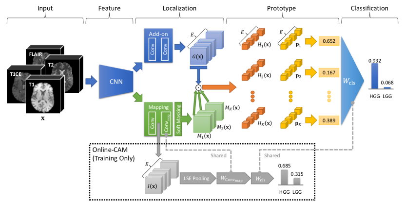
Figure 1: The overall architecture of MProtoNet. Online-CAM only occurs during training.

Inference Process

All layers are described in detail below. At a high level, MProtoNet delivers its prediction by comparing processed features with a set of learned prototypes $\mathbf{p}_{k}\subseteq\mathbf{P}$ ($k\in\left\{1\dots K\right\}$). Given input mpMRI data $\mathbf{x}$, the feature layer extracts the embedding features $F\left(\mathbf{x}\right)$. After that, $F\left(\mathbf{x}\right)$ is sent to both an add-on module and a mapping module in the localization layer to get high-level features $G\left(\mathbf{x}\right)$ and an attention map $M_{k}\left(\mathbf{x}\right)$ for each prototype $\mathbf{p}_{k}$. The dot-product result between $G\left(\mathbf{x}\right)$ and each $M_{k}\left(\mathbf{x}\right)$ is treated as the final features $H_{k}\left(\mathbf{x}\right)$ to be compared with each prototype $\mathbf{p}_{k}$. In the prototype layer, a similarity score $s\left(\mathbf{x},\mathbf{p}_{k}\right)$ between each pair of $H_{k}\left(\mathbf{x}\right)$ and $\mathbf{p}_{k}$ is calculated and sent to the classification layer to get the final prediction.

Feature Layer

The feature layer is a CNN module that performs feature extraction on the input mpMRI $\mathbf{x}\in\mathbb{R}^{4\times 128\times 128\times 96}$. ResNet He et al. (2016) is chosen as the backbone for its good performance on a wide variety of image tasks and relatively low model complexity. We directly replace 2D operations (such as convolutions) with 3D ones to make a 3D version of ResNet. Due to the need for localization at subsequent layers, we only use the layers up to the second building block of ResNet-152, resulting in a final output $F\left(\mathbf{x}\right)\in\mathbb{R}^{512\times 16\times 16\times 12}$ sent to the localization layer. Because it is difficult to find a suitable pre-trained version of 3D ResNet, the feature layer is trained from scratch.

Localization Layer

The localization layer has two branches that receive the same input $F\left(\mathbf{x}\right)$ from previous layer: an add-on module and a mapping module. The add-on module (following ProtoPNet Chen et al. (2019)) extracts high-level embedding features $G\left(\mathbf{x}\right)\in\mathbb{R}^{E\times 16\times 16\times 12}$, where $E$ is the number of embedding channels. The mapping module (modified from XProtoNet Kim et al. (2021)) outputs attention maps $M_{k}\left(\mathbf{x}\right)\in\mathbb{R}^{16\times 16\times 12}$ ($k\in\left\{1\dots K\right\}$) for localizing regions related to prototypes $\mathbf{p}_{k}$ ($k\in\left\{1\dots K\right\}$). The values of the attention maps $M_{k}\left(\mathbf{x}\right)$ are scaled into a range of $\left[0,1\right]$. To learn more accurate and sharper attention maps and reduce irrelevant background areas, we introduce differentiable soft masking Li et al. (2018) to sharpen the values of the attention maps $M_{k}^{0}\left(\mathbf{x}\right)$

$$M_{k}\left(\mathbf{x}\right)=\frac{1}{1+\exp\left(-\omega\left(M_{k}^{0}\left(\mathbf{x}\right)-\sigma\right)\right)},$$ (1)

where $\omega$ and $\sigma$ are hyper-parameters that are respectively set to be 10 and 0.5 (following Li et al. (2018)). The final features $H_{k}\left(\mathbf{x}\right)\in\mathbb{R}^{E\times 1\times 1\times 1}$ ($k\in\left\{1\dots K\right\}$) are obtained through

$$H_{k}\left(\mathbf{x}\right)=\frac{1}{16\times 16\times 12}\sum_{h,w,d}G_{h,w,d}\left(\mathbf{x}\right)\cdot M_{k,h,w,d}\left(\mathbf{x}\right),$$ (2)

where $h$, $w$ and $d$ are height, width and depth of the corresponding features. They represent the highly-activated regions of high-level features for the respective prototype $\mathbf{p}_{k}$.

Prototype and Classification Layers

The prototype layer stores a set of learned prototypes $\mathbf{p}_{k}\subseteq\mathbf{P}$ ($k\in\left\{1\dots K\right\}$), where $\mathbf{p}_{k}\in\mathbb{R}^{E\times 1\times 1\times 1}$. $K$ prototypes $\mathbf{p}_{k}\subseteq\mathbf{P}$ are evenly assigned to each class $c\in\left\{\mathrm{HGG,LGG}\right\}$. The common cosine similarity is used for the calculation of the similarity score between each pair of $H_{k}\left(\mathbf{x}\right)$ and $\mathbf{p}_{k}$

$$s\left(\mathbf{x},\mathbf{p}_{k}\right)=\frac{H_{k}\left(\mathbf{x}\right)\cdot\mathbf{p}_{k}}{\left\|H_{k}\left(\mathbf{x}\right)\right\|\left\|\mathbf{p}_{k}\right\|}.$$ (3)

Then, the similarity scores $s\left(\mathbf{x},\mathbf{p}_{k}\right)\subseteq\mathbf{S}$ ($k\in\left\{1\dots K\right\}$) are multiplied by the weight matrix $W_{\mathrm{cls}}\in\mathbb{R}^{K\times 2}$ in the classification layer to output the finally predicted probabilities $p\left(\mathbf{x}\right)$ for HGG and LGG (which are normalized using the softmax function).

2.3 Training and Loss Functions

The training of MProtoNet consists of three stages: (1) training of layers before the classification layer; (2) prototype reassignment; (3) training of the classification layer. See app:Training_Stages for details as they are the same as those employed in previous ProtoPNet variants. The following loss functions are used during these training stages: classification loss $\mathcal{L}_{\mathrm{cls}}$, cluster loss $\mathcal{L}_{\mathrm{clst}}$, separation loss $\mathcal{L}_{\mathrm{sep}}$, mapping loss $\mathcal{L}_{\mathrm{map}}$, online-CAM loss $\mathcal{L}_{\mathrm{OC}}$, and L1-regularization loss $\mathcal{L}_{\mathrm{L1}}$.

Because of the imbalanced distribution of class $c\in\left\{\mathrm{HGG,LGG}\right\}$ (HGG:LGG = 293:76), we use class weighted $\mathcal{L}_{\mathrm{cls}}$, $\mathcal{L}_{\mathrm{clst}}$ and $\mathcal{L}_{\mathrm{sep}}$ from XProtoNet Kim et al. (2021) but with a necessary transition from multi-label classification to multi-class classification. $\mathcal{L}_{\mathrm{map}}$ originates from the occurrence loss in XProtoNet Kim et al. (2021), while $\mathcal{L}_{\mathrm{L1}}$ originates from the L1 regularization term of the classification layer in ProtoPNet Chen et al. (2019).

Online-CAM Loss

In addition to soft masking and the mapping loss, an online-CAM loss is proposed here to assist localization of the attention maps by directly utilizing image-level labels during training of the attention module. Since the last convolution operation in the mapping module of the localization layer $\mathrm{Conv_{map}}$ is responsible for generating the attention maps, the intermediate features $I_{e}\left(\mathbf{x}\right)\subseteq\mathbf{I}\left(\mathbf{x}\right)$ ($e\in\left\{1\dots E\right\}$, $I_{e}\left(\mathbf{x}\right)\in\mathbb{R}^{16\times 16\times 12}$) right before the last convolution operation are made the feature sources of online-CAM (as shown in fig:Architecture). To obtain a class prediction directly from $I_{e}\left(\mathbf{x}\right)$, instead of employing average or max pooling, we choose log-sum-exp (LSE) pooling Pinheiro and Collobert (2015); Sun et al. (2016) which has shown improved convergence and localization performance

$$\mathrm{LSE}\left(I_{e}\left(\mathbf{x}\right)\right)=\frac{1}{r}\log\left[\frac{1}{16\times 16\times 12}\sum_{h,w,d}\exp\left(r\cdot I_{e,h,w,d}\left(\mathbf{x}\right)\right)\right],$$ (4)

where $h$, $w$ and $d$ are height, width and depth of the corresponding features; $r$ is a hyper-parameter that is set to be 10 (following Sun et al. (2016)). Then, $\mathrm{LSE}\left(\mathbf{I}\left(\mathbf{x}\right)\right)\in\mathbb{R}^{E}$ is consecutively multiplied by the weight matrix $W_{\mathrm{Conv_{map}}}\in\mathbb{R}^{E\times K}$ of $\mathrm{Conv_{map}}$ and the weight matrix $W_{\mathrm{cls}}\in\mathbb{R}^{K\times 2}$ in the classification layer, to obtain yet another predicted probability $p_{\mathrm{OC}}\left(\mathbf{x}\right)$ (which is different from the predicted probability $p\left(\mathbf{x}\right)$ in the classification layer). $\mathcal{L}_{\mathrm{OC}}$ is modified from $\mathcal{L}_{\mathrm{cls}}$

$$\aligned p_{\mathrm{OC}}\left(\mathbf{x}_{i}\right)&=\mathrm{Softmax}\left(\mathrm{LSE}\left(\mathbf{I}\left(\mathbf{x}_{i}\right)\right)W_{\mathrm{Conv_{map}}}W_{\mathrm{cls}}\right),\\ \mathcal{L}_{\mathrm{OC}}=\sum_{i}\frac{1}{N^{c}}\left(1-p_{\mathrm{OC}}^{c}\left(\mathbf{x}_{i}\right)\right)^{\gamma}\log p_{\mathrm{OC}}^{c}\left(\mathbf{x}_{i}\right),$$ (5)

where $i$ indexes the training samples, $N^{c}$ denotes the total number of training samples in class $c$ and $\gamma$ is a hyper-parameter that is set to be 2 (following Kim et al. (2021)). While the online-CAM loss $\mathcal{L}_{\mathrm{OC}}$ is useful during training, the corresponding predictions $p_{\mathrm{OC}}\left(\mathbf{x}_{i}\right)$ are not performed during inference.

3 Experiments and Results

3.1 Experimental Setup

In our experiments, since the class distribution in BraTS 2020 is highly imbalanced, we use the balanced accuracy (BAC) that is the macro-average of the recall scores of the two classes HGG and LGG to evaluate the classification performance. For the interpretability metrics, we focus on correctness and localization coherence as described in Nauta et al. (2023). The correctness of a model is evaluated by the normalized area under the incremental deletion curve Nauta et al. (2023), called the incremental deletion score (IDS). IDS measures how precisely an activation map reflects a model’s decision-making process (lower is better). The localization coherence is evaluated by the activation precision (AP) Barnett et al. (2021). AP measures the proportion of an activation map that intersects with the human-annotated label. See app:Evaluation_Metrics_for_Interpretability for detailed definitions of IDS and AP. To test a model’s performance under different training/test splits, stratified 5-fold cross-validation is applied throughout all experiments. See app:Hyper-parameters_During_Training for details of the hyper-parameters during training.

There are three models compared in our experiments: CNN (with GradCAM Selvaraju et al. (2017)), ProtoPNet Chen et al. (2019); Barnett et al. (2021) and XProtoNet Kim et al. (2021). For fair comparisons across models, all of them are reimplemented to share the same experimental settings as MProtoNet, except for the distinctions specified below.

CNN (with GradCAM)

The baseline CNN is built based on submodules of MProtoNet: the feature layer, the add-on module in the localization layer, and the classification layer. These submodules are marked as blue in fig:Architecture. The add-on module and the classification layer (with $W_{\mathrm{cls}}\in\mathbb{R}^{E\times 2}$) are directly connected with a global average pooling layer.

ProtoPNet

Compared to MProtoNet, the reimplemented ProtoPNet (adapted for 3D mpMRIs) lacks the mapping module in the localization layer and all associated loss functions. The similarity scores $s\left(\mathbf{x},\mathbf{p}_{k}\right)$ are calculated by directly comparing each location in $G\left(\mathbf{x}\right)$ with $\mathbf{p}_{k}$, followed by top-$\alpha$ average pooling (where $\alpha=1\%$) Barnett et al. (2021).

XProtoNet

MProtoNet is actually the reimplemented XProtoNet (adapted for 3D mpMRIs) with the addition of soft masking and the online-CAM loss.

3.2 Results

tab:Results shows all quantitative results from the 5-fold cross-validation experiments, including three versions of MProtoNet (A: without online-CAM loss, B: without soft masking, C: complete version). The results represent the contributions of all modalities since the fusion of modalities occurs at the very beginning. Given that MProtoNet is most similar to XProtoNet, 5-fold cross-validated paired Student’s t-tests (null hypothesis: paired results have identical means) against XProtoNet are performed on all results for MProtoNet A/B/C.

tab:Results Model Condition Classification Interpretability AM SM OC BAC IDS AP CNN (with GradCAM) $0.865\pm 0.026$ $0.112\pm 0.049$ $0.099\pm 0.030$ ProtoPNet $0.868\pm 0.032$ $0.609\pm 0.164$ $0.007\pm 0.001$ XProtoNet $\mathbf{0.870\pm 0.021}$ $0.170\pm 0.041$ $0.203\pm 0.030$ MProtoNet A $\underset{\left(p=0.929\right)}{0.868\pm 0.050}$ $\underset{\left(p=0.647\right)}{0.150\pm 0.088}$ $\underset{\left(p=0.004\right)}{0.568\pm 0.125}$ MProtoNet B $\underset{\left(p=0.360\right)}{0.865\pm 0.015}$ $\underset{\left(p=0.069\right)}{0.103\pm 0.020}$ $\underset{\left(p=0.963\right)}{0.204\pm 0.028}$ MProtoNet C $\underset{\left(p=0.516\right)}{0.858\pm 0.048}$ $\underset{\left(p=0.031\right)}{\mathbf{0.079\pm 0.034}}$ $\underset{\left(p<0.001\right)}{\mathbf{0.713\pm 0.058}}$

Table 1: A summary of all results in the form of [mean $\pm$ standard deviation] from 5-fold cross-validation. Bold indicates the best performance. For MProtoNet A/B/C, the $p$-value from the paired t-test against XProtoNet is shown under each result. Keys: AM – attention map, SM – soft masking, OC – online-CAM, BAC – balanced accuracy, IDS – incremental deletion score, AP – activation precision.

Comparing classification performance (BAC), there are no statistically significant differences among all models, most notably between MProtoNet A/B/C and XProtoNet. This is desirable as the same 3D ResNet backbone is shared across all models and appears to be well-suited for this task. The introduction of the interpretable components in our MProtoNet does not necessarily improve or hurt the classification performance. However, one of the most valuable outcomes is that it can provide case-based prototypical explanations during inference, as shown in fig:Case-Based_Reasoning.

fig:Case-Based_Reasoning

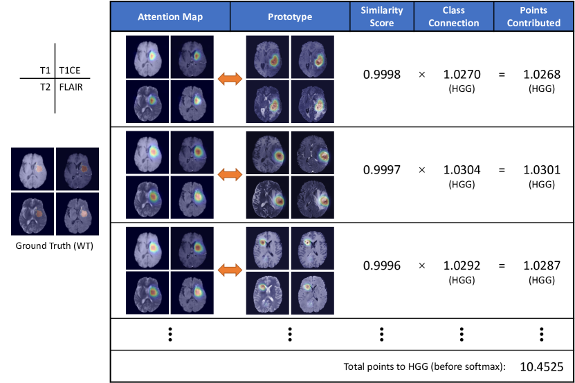
Figure 2: Demonstration of the case-based reasoning in MProtoNet. It can provide case-based prototypical explanations with both attention maps and similarity scores.

The complete version MProtoNet C achieves the best performance in terms of both correctness (IDS) and localization coherence (AP), excelling in interpretability. Specifically, both soft masking and the online-CAM loss are very important for statistically significant improvements in IDS ($p=0.031$) and AP ($p<0.001$) over XProtoNet, resulting in the best IDS of $0.079\pm 0.034$ and the best AP of $0.713\pm 0.058$. Since we do not use any annotation information during training, the poor performance of the original ProtoPNet (even with top-$\alpha$ average pooling) is expected as previously shown in Barnett et al. (2021). fig:Localization_Coherence clearly shows the improvement of MProtoNet C over all other models in terms of localization coherence. See app:More_Visualization_Examples_of_Localization_Coherence for more visualization examples.

fig:Localization_Coherence

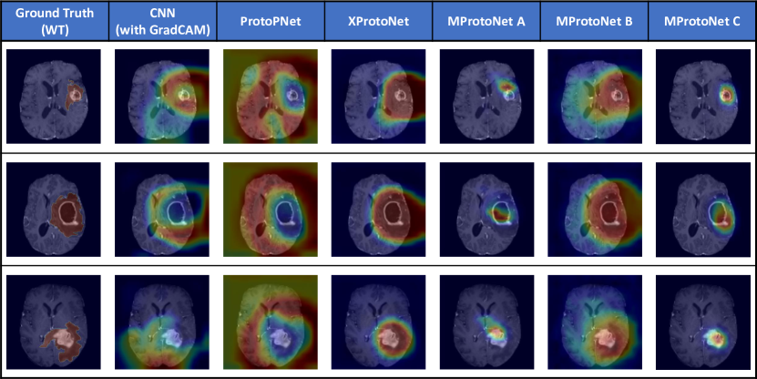
Figure 3: Visualization examples of the localization coherence results from different methods (shown with the T1CE modality). MProtoNet C clearly outperforms all other models, showing the importance of both soft masking and the online-CAM loss.

4 Conclusions and Future Work

In this work, we propose MProtoNet to apply case-based interpretable deep learning to brain tumor classification with 3D mpMRIs, targeting a goal of precisely localizing attention regions. The proposed new attention module with soft masking and online-CAM loss helps MProtoNet achieve the best performance on interpretability in terms of both correctness and localization coherence. Meanwhile, the classification accuracy is on par with baseline CNN and other ProtoPNet variants specifically designed for medical images. No annotation information is required during training, showing the great potential of MProtoNet on 3D medical image applications wherein fine-grained annotation labels are difficult to obtain. The ability to simultaneously output attribution maps and case-based prototypical explanations also makes MProtoNet a potential alternative to current 3D CNNs in many 3D medical imaging tasks.

There are several potential aspects for future improvements over MProtoNet. Firstly, rather than fixed assignments of prototypes before and after training, a dynamic or even shared assignment Rymarczyk et al. (2021, 2022) might be more suitable for some medical image applications. Secondly, instead of fusing the multiple modalities at the beginning, we shall also test fusion at the end to analyze each individual modality like some gradient-based methods Jin et al. (2022, 2023). Lastly, potential combinations with other interpretable methods such as concept-based models Koh et al. (2020) might further improve MProtoNet’s interpretability on much more complicated medical image applications.

This study was supported by the National Natural Science Foundation of China (62071210); the Shenzhen Science and Technology Program (RCYX20210609103056042); the Shenzhen Science and Technology Innovation Committee (KCXFZ2020122117340001); the Shenzhen Basic Research Program (JCYJ20200925153847004, JCYJ20190809120205578); the Natural Sciences and Engineering Research Council of Canada.

Appendix A Preprocessing and Data Augmentation

A.1 Preprocessing

All mpMRI data in BraTS 2020 go through a standardized preprocessing pipeline including co-registration to a common anatomical template (SRI24 Rohlfing et al. (2010)), resampling to a 1×1×1 mm³ resolution, and skull-stripping. After original preprocessing, each image has a size of 240×240×155 voxels (1×1×1 mm³ resolution). The images are cropped around the borders to 192×192×144 voxels, and then further down-sampled to 128×128×96 voxels (1.5×1.5×1.5 mm³ resolution) to enable efficient training on GPUs. After that, intensity normalization is performed on each mpMRI image of a specific modality by subtracting the individual mean and dividing by the individual standard deviation.

A.2 Data Augmentation

During training, we follow the online data augmentation pipeline of nnU-Net Isensee et al. (2021), which has already been successfully applied to many 3D medical imaging tasks, to overcome the limited size issue of the training data. The augmentations are applied stochastically in the following sequence: (1) rotation and scaling; (2) Gaussian noise; (3) Gaussian blur; (4) brightness augmentation; (5) contrast augmentation; (6) simulation of low resolution; (7) gamma augmentation; (8) mirroring. Detailed parameters for each augmentation operation can be found in Isensee et al. (2021).

Appendix B Training Stages

Stage-1: Training of Layers Before the Classification Layer

During the first training stage, we train all layers except the classification layer to obtain a meaningful embedding space for the prototypes. The overall loss function is

$$\mathcal{L}_{\textrm{stage-1}}=\lambda_{\mathrm{cls}}\mathcal{L}_{\mathrm{cls}}+\lambda_{\mathrm{clst}}\mathcal{L}_{\mathrm{clst}}+\lambda_{\mathrm{sep}}\mathcal{L}_{\mathrm{sep}}+\lambda_{\mathrm{map}}\mathcal{L}_{\mathrm{map}}+\lambda_{\mathrm{OC}}\mathcal{L}_{\mathrm{OC}},$$ (6)

where $\lambda_{\mathrm{cls}}$, $\lambda_{\mathrm{clst}}$, $\lambda_{\mathrm{sep}}$, $\lambda_{\mathrm{map}}$ and $\lambda_{\mathrm{OC}}$ are coefficients of respective losses.

Stage-2: Prototype Reassignment

To achieve the goal of case-based reasoning, i.e., to be able to view each prototype as a specific patch of a training sample, we need to replace the representation of each prototype $\mathbf{p}_{k}\subseteq\mathbf{P}$ ($k\in\left\{1\dots K\right\}$) with the nearest processed feature $H_{k}\left(\mathbf{x}\right)$ (without any online data augmentation for $\mathbf{x}$) after several iterations in stage-1. Therefore, we can treat the corresponding training sample $\mathbf{x}$ with the attention map $M_{k}\left(\mathbf{x}\right)$ superimposed on it as the visualization of prototype $\mathbf{p}_{k}$.

Stage-3: Training of the Classification Layer

After reassigning prototypes in stage-2, we train the classification layer separately to learn a weight matrix $W_{\mathrm{cls}}\in\mathbb{R}^{K\times 2}$ that represents the contributions of the prototypes for classification without changing their representation. The overall loss function is

$$\mathcal{L}_{\textrm{stage-3}}=\lambda_{\mathrm{cls}}\mathcal{L}_{\mathrm{cls}}+\lambda_{\mathrm{L1}}\mathcal{L}_{\mathrm{L1}},$$ (7)

where $\lambda_{\mathrm{cls}}$ and $\lambda_{\mathrm{L1}}$ are coefficients of respective losses.

Appendix C Evaluation Metrics for Interpretability

C.1 Correctness: Incremental Deletion Score (IDS)

Incremental deletion Nauta et al. (2023) is a commonly adopted method to assess the interpretability of an activation map by incrementally deleting features (e.g., replaced with 0) in the input according to the activation map values (from high values to low values). The top-valued features are deleted at the beginning. If the curve of classification metric drops faster, the activation map more precisely reflects a model’s decision-making process. To quantify the sharpness of the curve of incremental deletion, incremental deletion score (IDS) is defined here as the normalized area under the curve and within the bounds of start and end, as shown in fig:IDS. The lower the IDS, the better performance in terms of correctness.

fig:IDS

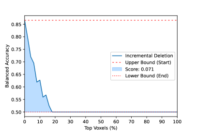
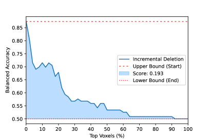
Figure 4: Demonstration of the incremental deletion score (IDS).

C.2 Localization Coherence: Activation Precision (AP)

The localization coherence is evaluated by the activation precision (AP) Barnett et al. (2021)

$$\mathrm{AP}=\frac{\left|H\left(\mathbf{x}\right)\cap T\left(\mathrm{UpSample}\left(M\left(\mathbf{x}\right)\right)\right)\right|}{\left|T\left(\mathrm{UpSample}\left(M\left(\mathbf{x}\right)\right)\right)\right|},$$ (8)

where $H\left(\mathbf{x}\right)$ is the human-annotated label for the WT region of $\mathbf{x}$, $M\left(\mathbf{x}\right)$ is the activation map for $\mathbf{x}$ and $T\left(\cdot\right)$ is a threshold function. In this work, $T\left(\cdot\right)$ is set to be a binary function with the threshold 0.5. For MProtoNet as well as XProtoNet

$$M\left(\mathbf{x}\right)=\frac{1}{K^{c}}\sum M_{k}^{c}\left(\mathbf{x}\right),$$ (9)

where $c$ denotes the correct class of $\mathbf{x}$ and $K^{c}$ denotes the total number of prototypes assigned to class $c$. For CNN (with GradCAM), GradCAM is used to generate the activation map $M\left(\mathbf{x}\right)$ from the last convolution layer of the CNN after training. For ProtoPNet, the average of the intermediate results right before top-$\alpha$ average pooling is used as the activation map $M\left(\mathbf{x}\right)$ (following Barnett et al. (2021)).

Appendix D Hyper-parameters During Training

Following some latest practices from Liu et al. (2022), MProtoNet is trained by the AdamW optimizer with a baseline learning rate of 0.001 and a weight decay coefficient of 0.01. During each cross-validation iteration, MProtoNet is trained for 100 epochs (stage-1) with a batch size of 32 and a specific learning rate scheduler (linear warm-up for the first 20 epochs and cosine annealing for the remaining 80 epochs). After every 10 epochs of stage-1, there is a step of stage-2 (with only prototype reassignment) and 10 epochs of stage-3 (where MProtoNet is trained by the Adam optimizer with a constant learning rate of 0.001). The number of embedding channels $E$ is set to be 128 and the number of prototypes $K$ is set to be 30 (15 for each class). The coefficients of loss functions are set as follows: $\lambda_{\mathrm{cls}}$ as 1, $\lambda_{\mathrm{clst}}$ as 0.8, $\lambda_{\mathrm{sep}}$ as 0.08, $\lambda_{\mathrm{map}}$ as 0.5, $\lambda_{\mathrm{OC}}$ as 0.05 and $\lambda_{\mathrm{L1}}$ as 0.01.

Appendix E More Visualization Examples of Localization Coherence

fig:More_Localization_Coherence

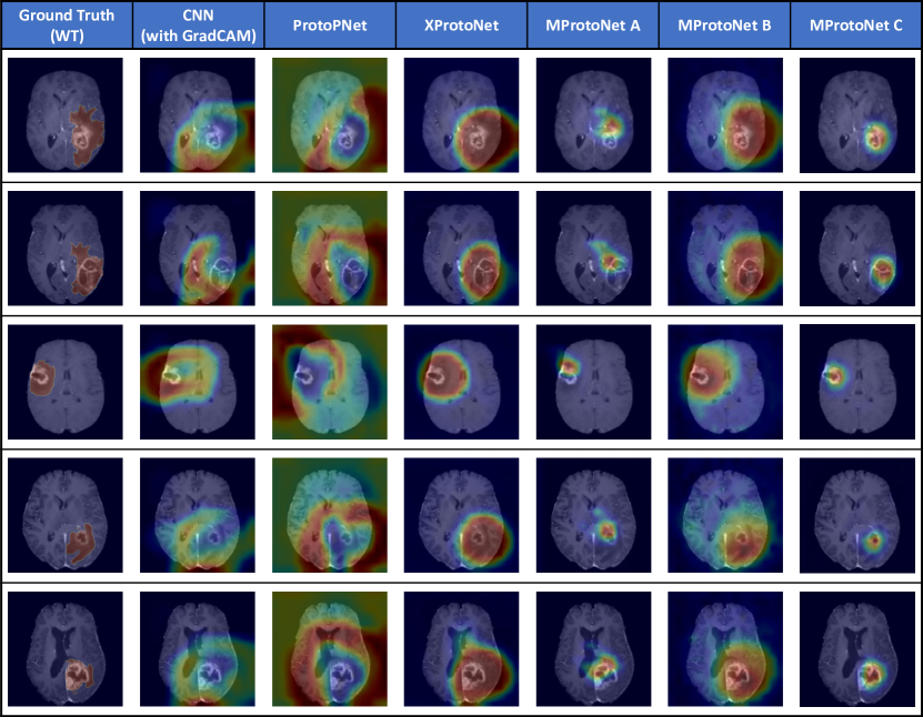
Figure 5: More visualization examples of the localization coherence results from different methods (shown with the T1CE modality).

References

- Adebayo et al. (2018) Julius Adebayo, Justin Gilmer, Michael Muelly, Ian Goodfellow, Moritz Hardt, and Been Kim. Sanity checks for saliency maps. In Advances in Neural Information Processing Systems, volume 31, Montreal, Canada, December 2018. Curran Associates, Inc. URL \urlhttps://proceedings.neurips.cc/paper/2018/hash/294a8ed24b1ad22ec2e7efea049b8737-Abstract.html.
- Amyar et al. (2022) Amine Amyar, Romain Modzelewski, Pierre Vera, Vincent Morard, and Su Ruan. Weakly supervised tumor detection in PET using class response for treatment outcome prediction. Journal of Imaging, 8(5):130, May 2022. 10.3390/jimaging8050130.
- Barnett et al. (2021) Alina Jade Barnett, Fides Regina Schwartz, Chaofan Tao, Chaofan Chen, Yinhao Ren, Joseph Y. Lo, and Cynthia Rudin. A case-based interpretable deep learning model for classification of mass lesions in digital mammography. Nature Machine Intelligence, 3(12):1061–1070, December 2021. 10.1038/s42256-021-00423-x.
- Chen et al. (2019) Chaofan Chen, Oscar Li, Chaofan Tao, Alina Jade Barnett, Jonathan Su, and Cynthia Rudin. This looks like that: Deep learning for interpretable image recognition. In Advances in Neural Information Processing Systems, volume 32, Vancouver, Canada, December 2019. Curran Associates, Inc. URL \urlhttps://proceedings.neurips.cc/paper/2019/hash/adf7ee2dcf142b0e11888e72b43fcb75-Abstract.html.
- DeGrave et al. (2021) Alex J. DeGrave, Joseph D. Janizek, and Su-In Lee. AI for radiographic COVID-19 detection selects shortcuts over signal. Nature Machine Intelligence, 3(7):610–619, July 2021. 10.1038/s42256-021-00338-7.
- Donnelly et al. (2022) Jon Donnelly, Alina Jade Barnett, and Chaofan Chen. Deformable ProtoPNet: An interpretable image classifier using deformable prototypes. In 2022 IEEE/CVF Conference on Computer Vision and Pattern Recognition (CVPR), pages 10255–10265, New Orleans, United States, June 2022. IEEE. 10.1109/CVPR52688.2022.01002.
- Fukui et al. (2019) Hiroshi Fukui, Tsubasa Hirakawa, Takayoshi Yamashita, and Hironobu Fujiyoshi. Attention branch network: Learning of attention mechanism for visual explanation. In 2019 IEEE/CVF Conference on Computer Vision and Pattern Recognition (CVPR), pages 10697–10706, Long Beach, United States, June 2019. IEEE. 10.1109/CVPR.2019.01096.
- Geirhos et al. (2020) Robert Geirhos, Jörn-Henrik Jacobsen, Claudio Michaelis, Richard Zemel, Wieland Brendel, Matthias Bethge, and Felix A. Wichmann. Shortcut learning in deep neural networks. Nature Machine Intelligence, 2(11):665–673, November 2020. 10.1038/s42256-020-00257-z.
- He et al. (2016) Kaiming He, Xiangyu Zhang, Shaoqing Ren, and Jian Sun. Deep residual learning for image recognition. In 2016 IEEE Conference on Computer Vision and Pattern Recognition (CVPR), pages 770–778, Las Vegas, United States, June 2016. IEEE. 10.1109/CVPR.2016.90.
- Isensee et al. (2021) Fabian Isensee, Paul F. Jaeger, Simon A. A. Kohl, Jens Petersen, and Klaus H. Maier-Hein. nnU-Net: A self-configuring method for deep learning-based biomedical image segmentation. Nature Methods, 18(2):203–211, February 2021. 10.1038/s41592-020-01008-z.
- Jin et al. (2022) Weina Jin, Xiaoxiao Li, and Ghassan Hamarneh. Evaluating explainable AI on a multi-modal medical imaging task: Can existing algorithms fulfill clinical requirements? Proceedings of the AAAI Conference on Artificial Intelligence, 36(11):11945–11953, June 2022. 10.1609/aaai.v36i11.21452.
- Jin et al. (2023) Weina Jin, Xiaoxiao Li, Mostafa Fatehi, and Ghassan Hamarneh. Guidelines and evaluation of clinical explainable AI in medical image analysis. Medical Image Analysis, 84:102684, February 2023. 10.1016/j.media.2022.102684.
- Kim et al. (2021) Eunji Kim, Siwon Kim, Minji Seo, and Sungroh Yoon. XProtoNet: Diagnosis in chest radiography with global and local explanations. In 2021 IEEE/CVF Conference on Computer Vision and Pattern Recognition (CVPR), pages 15714–15723, Nashville, United States, June 2021. IEEE. 10.1109/CVPR46437.2021.01546.
- Koh et al. (2020) Pang Wei Koh, Thao Nguyen, Yew Siang Tang, Stephen Mussmann, Emma Pierson, Been Kim, and Percy Liang. Concept bottleneck models. In Proceedings of the 37th International Conference on Machine Learning, volume 119 of Proceedings of Machine Learning Research, pages 5338–5348, Virtual, July 2020. PMLR. URL \urlhttps://proceedings.mlr.press/v119/koh20a.html.
- Li et al. (2018) Kunpeng Li, Ziyan Wu, Kuan-Chuan Peng, Jan Ernst, and Yun Fu. Tell me where to look: Guided attention inference network. In 2018 IEEE/CVF Conference on Computer Vision and Pattern Recognition, pages 9215–9223, Salt Lake City, United States, June 2018. IEEE. 10.1109/CVPR.2018.00960.
- Liu et al. (2022) Zhuang Liu, Hanzi Mao, Chao-Yuan Wu, Christoph Feichtenhofer, Trevor Darrell, and Saining Xie. A ConvNet for the 2020s. In 2022 IEEE/CVF Conference on Computer Vision and Pattern Recognition (CVPR), pages 11966–11976, New Orleans, United States, June 2022. IEEE. 10.1109/CVPR52688.2022.01167.
- Menze et al. (2015) Bjoern H. Menze, Andras Jakab, Stefan Bauer, Jayashree Kalpathy-Cramer, Keyvan Farahani, Justin Kirby, Yuliya Burren, Nicole Porz, Johannes Slotboom, Roland Wiest, Levente Lanczi, Elizabeth Gerstner, Marc-André Weber, Tal Arbel, Brian B. Avants, Nicholas Ayache, Patricia Buendia, D. Louis Collins, Nicolas Cordier, Jason J. Corso, Antonio Criminisi, Tilak Das, Hervé Delingette, Çağatay Demiralp, Christopher R. Durst, Michel Dojat, Senan Doyle, Joana Festa, Florence Forbes, Ezequiel Geremia, Ben Glocker, Polina Golland, Xiaotao Guo, Andac Hamamci, Khan M. Iftekharuddin, Raj Jena, Nigel M. John, Ender Konukoglu, Danial Lashkari, José António Mariz, Raphael Meier, Sérgio Pereira, Doina Precup, Stephen J. Price, Tammy Riklin Raviv, Syed M. S. Reza, Michael Ryan, Duygu Sarikaya, Lawrence Schwartz, Hoo-Chang Shin, Jamie Shotton, Carlos A. Silva, Nuno Sousa, Nagesh K. Subbanna, Gabor Szekely, Thomas J. Taylor, Owen M. Thomas, Nicholas J. Tustison, Gozde Unal, Flor Vasseur, Max Wintermark, Dong Hye Ye, Liang Zhao, Binsheng Zhao, Darko Zikic, Marcel Prastawa, Mauricio Reyes, and Koen Van Leemput. The multimodal brain tumor image segmentation benchmark (BRATS). IEEE Transactions on Medical Imaging, 34(10):1993–2024, October 2015. 10.1109/TMI.2014.2377694.
- Nauta et al. (2023) Meike Nauta, Jan Trienes, Shreyasi Pathak, Elisa Nguyen, Michelle Peters, Yasmin Schmitt, Jörg Schlötterer, Maurice van Keulen, and Christin Seifert. From anecdotal evidence to quantitative evaluation methods: A systematic review on evaluating explainable AI. ACM Computing Surveys, February 2023. 10.1145/3583558.
- Ouyang et al. (2021) Xi Ouyang, Srikrishna Karanam, Ziyan Wu, Terrence Chen, Jiayu Huo, Xiang Sean Zhou, Qian Wang, and Jie-Zhi Cheng. Learning hierarchical attention for weakly-supervised chest X-ray abnormality localization and diagnosis. IEEE Transactions on Medical Imaging, 40(10):2698–2710, October 2021. 10.1109/TMI.2020.3042773.
- Pinheiro and Collobert (2015) Pedro O. Pinheiro and Ronan Collobert. From image-level to pixel-level labeling with convolutional networks. In 2015 IEEE Conference on Computer Vision and Pattern Recognition (CVPR), pages 1713–1721, Boston, United States, June 2015. IEEE. 10.1109/CVPR.2015.7298780.
- Rohlfing et al. (2010) Torsten Rohlfing, Natalie M. Zahr, Edith V. Sullivan, and Adolf Pfefferbaum. The SRI24 multichannel atlas of normal adult human brain structure. Human Brain Mapping, 31(5):798–819, May 2010. 10.1002/hbm.20906.
- Rudin (2019) Cynthia Rudin. Stop explaining black box machine learning models for high stakes decisions and use interpretable models instead. Nature Machine Intelligence, 1(5):206–215, May 2019. 10.1038/s42256-019-0048-x.
- Rymarczyk et al. (2021) Dawid Rymarczyk, Łukasz Struski, Jacek Tabor, and Bartosz Zieliński. ProtoPShare: Prototypical parts sharing for similarity discovery in interpretable image classification. In Proceedings of the 27th ACM SIGKDD Conference on Knowledge Discovery & Data Mining, pages 1420–1430, Singapore, August 2021. ACM. 10.1145/3447548.3467245.
- Rymarczyk et al. (2022) Dawid Rymarczyk, Łukasz Struski, Michał Górszczak, Koryna Lewandowska, Jacek Tabor, and Bartosz Zieliński. Interpretable image classification with differentiable prototypes assignment. In Computer Vision – ECCV 2022, volume 13672 of Lecture Notes in Computer Science, pages 351–368, Tel Aviv, Israel, October 2022. Springer. 10.1007/978-3-031-19775-8_21.
- Selvaraju et al. (2017) Ramprasaath R. Selvaraju, Michael Cogswell, Abhishek Das, Ramakrishna Vedantam, Devi Parikh, and Dhruv Batra. Grad-CAM: Visual explanations from deep networks via gradient-based localization. In 2017 IEEE International Conference on Computer Vision (ICCV), pages 618–626, Venice, Italy, October 2017. IEEE. 10.1109/ICCV.2017.74.
- Sun et al. (2016) Chen Sun, Manohar Paluri, Ronan Collobert, Ram Nevatia, and Lubomir Bourdev. ProNet: Learning to propose object-specific boxes for cascaded neural networks. In 2016 IEEE Conference on Computer Vision and Pattern Recognition (CVPR), pages 3485–3493, Las Vegas, United States, June 2016. IEEE. 10.1109/CVPR.2016.379.
- Wang et al. (2021) Jiaqi Wang, Huafeng Liu, Xinyue Wang, and Liping Jing. Interpretable image recognition by constructing transparent embedding space. In 2021 IEEE/CVF International Conference on Computer Vision (ICCV), pages 875–884, Montreal, Canada, October 2021. IEEE. 10.1109/ICCV48922.2021.00093.
- Zhou et al. (2016) Bolei Zhou, Aditya Khosla, Agata Lapedriza, Aude Oliva, and Antonio Torralba. Learning deep features for discriminative localization. In 2016 IEEE Conference on Computer Vision and Pattern Recognition (CVPR), pages 2921–2929, Las Vegas, United States, June 2016. IEEE. 10.1109/CVPR.2016.319.
- Zhou et al. (2021) S. Kevin Zhou, Hayit Greenspan, Christos Davatzikos, James S. Duncan, Bram van Ginneken, Anant Madabhushi, Jerry L. Prince, Daniel Rueckert, and Ronald M. Summers. A review of deep learning in medical imaging: Imaging traits, technology trends, case studies with progress highlights, and future promises. Proceedings of the IEEE, 109(5):820–838, May 2021. 10.1109/JPROC.2021.3054390.
- Zhou et al. (2018) Yanzhao Zhou, Yi Zhu, Qixiang Ye, Qiang Qiu, and Jianbin Jiao. Weakly supervised instance segmentation using class peak response. In 2018 IEEE/CVF Conference on Computer Vision and Pattern Recognition, pages 3791–3800, Salt Lake City, United States, June 2018. IEEE. 10.1109/CVPR.2018.00399.